Magnetic field direction and lunar swirl morphology:Insights from Airy and Reiner Gamma
Doug Hemingway1 and Ian Garrick-Bethell1,2
Received 21 June 2012; revised 23 August 2012; accepted 30 August 2012; published 30 October 2012.
[1] Many of the Moon’s crustal magnetic anomalies are accompanied by high albedofeatures known as swirls. A leading hypothesis suggests that swirls are formed where crustalmagnetic anomalies, acting as mini magnetospheres, shield portions of the surface fromthe darkening effects of solar wind ion bombardment, thereby leaving patches that appearbright compared with their surroundings. If this hypothesis is correct, then magnetic fielddirection should influence swirl morphology. Using Lunar Prospector magnetometerdata and Clementine reflectance mosaics, we find evidence that bright regions correspondwith dominantly horizontal magnetic fields at Reiner Gamma and that vertical magneticfields are associated with the intraswirl dark lane at Airy. We use a genetic search algorithmto model the distributions of magnetic source material at both anomalies, and we showthat source models constrained by the observed albedo pattern (i.e., strongly horizontalsurface fields in bright areas, vertical surface fields in dark lanes) produce fields that areconsistent with the Lunar Prospector magnetometer measurements. These findings supportthe solar wind deflection hypothesis and may help to explain not only the general formof swirls, but also the finer aspects of their morphology. Our source models may also beused to make quantitative predictions of the near surface magnetic field, which mustultimately be tested with very low altitude spacecraft measurements. If our predictions arecorrect, our models could have implications for the structure of the underlying magneticmaterial and the nature of the magnetizing field.
Citation: Hemingway, D., and I. Garrick-Bethell (2012), Magnetic field direction and lunar swirl morphology: Insights fromAiry and Reiner Gamma, J. Geophys. Res., 117, E10012, doi:10.1029/2012JE004165.
1. Introduction
1.1. Background
[2] Although the Moon does not now possess a globalmagnetic field [Ness et al., 1967], remanent crustal magne-tization has been identified on the surface and several stableregional magnetic fields have been detected from orbit [Dyalet al., 1970; Coleman et al., 1972; Lin, 1979; Lin et al., 1998;Hood et al., 2001]. Curiously, many, but not all of thesecrustal magnetic anomalies are accompanied by sinuouspatterns of anomalously high surface reflectance known asswirls [Hood et al., 1979; Hood and Williams, 1989;Richmond et al., 2005; Blewett et al., 2011].[3] Compared with their surroundings, swirls are optically
immature, exhibit spectrally distinct space weathering trends
[Garrick-Bethell et al., 2011], and are depleted in hydroxylmolecules [Kramer et al., 2011]. Swirls appear to overprintlocal topography, having no detectable topographic or tex-tural expression of their own [Neish et al., 2011]. So far notidentified anywhere else in the solar system, swirls areunique natural laboratories where space weathering andcrustal magnetism intersect. As such, their study could helpaddress important questions in lunar science including theMoon’s dynamo history [Garrick-Bethell et al., 2009;Dwyeret al., 2011; Le Bars et al., 2011], the relative influences ofsolar wind and micrometeoroid bombardment on spaceweathering [Hapke, 2001; Vernazza et al., 2009], and theproduction and distribution of water over the lunar surface[Pieters et al., 2009; Kramer et al., 2011].[4] Electrostatic migration of dust has been proposed as a
possible mechanism for swirl formation [Garrick-Bethellet al., 2011], as have meteoroid or comet impacts [Schultzand Srnka, 1980; Pinet et al., 2000; Starukhina andShkuratov, 2004]. Another model suggests that crustal mag-netic fields act as mini magnetospheres, deflecting the solarwind and protecting portions of the surface from the opticalmaturation and darkening effects of proton bombardment[Hood and Schubert, 1980; Hood and Williams, 1989]. Thispaper aims to make and test predictions based on this solarwind deflection model for swirl formation.
1Earth and Planetary Sciences, University of California, Santa Cruz,California, USA.
2School of Space Research, Kyung Hee University, Yongin, SouthKorea.
Corresponding author: D. Hemingway, Earth and Planetary Sciences,University of California, 1156 High St., Santa Cruz, CA 95064, USA.([email protected])
JOURNAL OF GEOPHYSICAL RESEARCH, VOL. 117, E10012, doi:10.1029/2012JE004165, 2012
E10012 1 of 19
1.2. Predicted Influence of Magnetic Field Direction
[5] The solar wind deflection model suggests that solarwind ions are magnetically deflected due to the Lorentzforce. Neglecting the induced electric field, the cross productof particle velocity and magnetic field in the Lorentz Lawmeans the magnetic deflection force is maximized whenparticle velocity is perpendicular to the magnetic field andzero when it is parallel. Hence, if the high albedo of swirls isthe result of inhibited space weathering due to magneticdeflection of solar wind ions, magnetic field direction shouldinfluence swirl morphology. While the solar wind incidenceangle varies, the ion flux at the surface and thus any dark-ening effects will be greatest when the ion trajectories arevertical. We therefore predict that portions of the crust thatare shielded by dominantly horizontal magnetic fields shouldreceive maximum protection from the solar wind while por-tions of the crust associated with vertically oriented magneticfields should experience protection only at low solar windincidence angles, when darkening effects would be minimalanyway. This suggests that the magnetic fields directly over
the bright swirls should be dominantly horizontal and thataway from swirls and in the intraswirl dark lanes, the fieldsmay be either closer to vertical or too weak to offer the sur-face any protection from solar wind darkening.[6] Because magnetic field strength decreases rapidly with
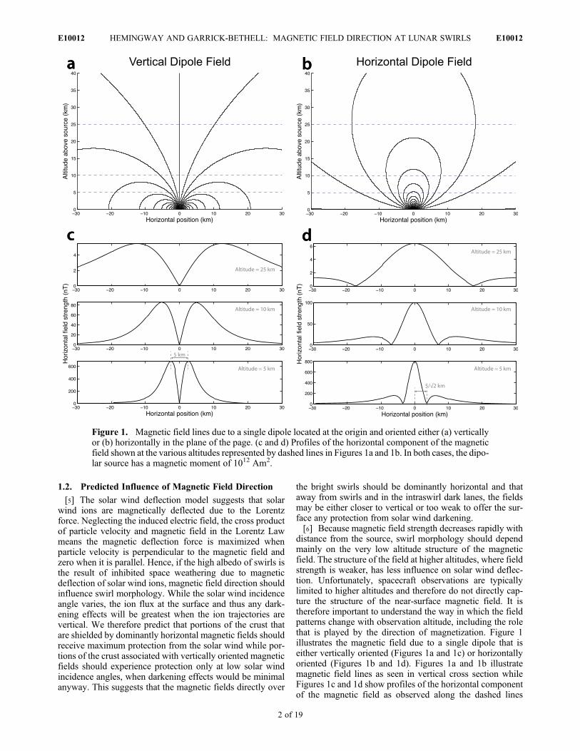
distance from the source, swirl morphology should dependmainly on the very low altitude structure of the magneticfield. The structure of the field at higher altitudes, where fieldstrength is weaker, has less influence on solar wind deflec-tion. Unfortunately, spacecraft observations are typicallylimited to higher altitudes and therefore do not directly cap-ture the structure of the near-surface magnetic field. It istherefore important to understand the way in which the fieldpatterns change with observation altitude, including the rolethat is played by the direction of magnetization. Figure 1illustrates the magnetic field due to a single dipole that iseither vertically oriented (Figures 1a and 1c) or horizontallyoriented (Figures 1b and 1d). Figures 1a and 1b illustratemagnetic field lines as seen in vertical cross section whileFigures 1c and 1d show profiles of the horizontal componentof the magnetic field as observed along the dashed lines
Figure 1. Magnetic field lines due to a single dipole located at the origin and oriented either (a) verticallyor (b) horizontally in the plane of the page. (c and d) Profiles of the horizontal component of the magneticfield shown at the various altitudes represented by dashed lines in Figures 1a and 1b. In both cases, the dipo-lar source has a magnetic moment of 1012 Am2.
HEMINGWAY AND GARRICK-BETHELL: MAGNETIC FIELD DIRECTION AT LUNAR SWIRLS E10012E10012
2 of 19
shown in Figures 1a and 1b (in both cases, the model dipoleis placed at the origin and arbitrarily assigned a magneticmoment of 1012 Am2). Directly over the vertically orienteddipole, field lines are vertical at any altitude (Figure 1a).Peaks in the horizontal field strength appear to either side andare separated by a distance equal to the observation altitude(Figure 1c). Directly over the horizontally oriented dipole,field lines are horizontal at any altitude (Figure 1b). As theobserver moves along an axis parallel to the dipole direction,horizontal field strength decreases, reaching zero (i.e., verti-cal field lines) at a horizontal distance of 1/√2 times theobservation altitude, before temporarily increasing againslightly (Figure 1d). Appendix A gives a quantitative treat-ment of the way in which magnetic fields vary with positionrelative to the source.[7] Our study uses Lunar Prospector magnetometer data
collected at altitudes of�18 km and higher. While we cannotmeasure the magnetic field structure below these altitudes,we can distinguish between vertically and horizontally ori-ented magnetizations (we assume that strong crustal mag-netic anomalies are approximately dipolar). This means wecan select anomalies exhibiting orientations that allow us totest our predictions. Specifically, we can look for intraswirldark lanes at an anomaly with approximately vertical mag-netization because, in that case, field lines should appearvertical at any altitude over the dark lane (Figures 1a and 1c).Likewise, we can look for a correlation between high albedoand strongly horizontal fields at anomalies with approxi-mately horizontal magnetization because field lines at suchanomalies should appear horizontal over the brightest areasregardless of observation altitude (Figures 1b and 1d). Wefind that the Airy anomaly is similar to the case illustrated inFigures 1a and 1c while the Reiner Gamma anomaly is sim-ilar to the case illustrated in Figures 1b and 1d.
2. Data Processing
2.1. Lunar Prospector Magnetometer Data
[8] Our study uses Lunar Prospector 3-axis magnetometermeasurements (level 1B data) obtained from NASA’s Plan-etary Data System (ppi.pds.nasa.gov). Two distinct approa-ches are available for producing maps of crustal magneticfields from orbital measurements. One involves direct map-ping using data selected from a sequence of orbits that crossthe region of interest [Hood et al., 1981, 2001], resulting inmaps of the field at the spacecraft altitude, while the otherinvolves developing a global spherical harmonic model andusing it to produce maps at arbitrary altitudes [Purucker andNicholas, 2010]. The spherical harmonic models are wellsuited to global mapping and have the advantages of auto-matically accounting for varying spacecraft altitudes andguaranteeing that the mapped field is a potential field. Todate, the best available spherical harmonic models extendto degree 170, corresponding to a horizontal wavelength of�64 km [Purucker and Nicholas, 2010]. However, becausewe are interested in small-scale swirl morphology, we insteademploy a direct mapping technique similar to that of Hoodet al. [2001], allowing us to map features at wavelengthscomparable with the spacecraft altitude (as low as �18 km).As discussed byHood [2011], the direct mapping approach issuitable for regional mapping and has several advantagesincluding that it allows us to perform model fitting directly to
the minimally processed magnetometer measurements ratherthan to a derived field model. While we focus here on directmapping, we did compare our maps against maps we derivedfrom the Purucker and Nicholas [2010] model coefficients.We found that in the latter, crustal anomaly fields appearmorphologically similar to the same features in our maps, butare typically broader in horizontal extent and exhibit lowerfield strength.[9] Each of our maps incorporates data from a sequence of
consecutive orbits that cross the anomaly of interest. Thepolar orbiting spacecraft obtained global coverage twice eachlunation, with consecutive orbits spaced �1 degree in lon-gitude (�30 km at the equator) and with along-track mea-surements recorded at 5-s intervals, corresponding to �8 kmspacing in latitude. In order to capture the undisturbed signalof the crustal magnetic anomalies, avoiding times when thefield is distorted by the impinging solar wind [Kurata et al.,2005; Purucker, 2008], we use only those magnetometermeasurements collected when the Moon was protected fromsolar wind while passing through the Earth’s magnetotail(excluding times when the field was disturbed by the plasmasheet) or when the Moon was in the solar wind but thespacecraft was in the lunar wake (on the dark side of theMoon and away from the terminator by at least 20�). Weexamined data from the lowest (<50 km) altitude phaseof the mission, between February and July 1999 (the finalsix months of the mission). The upper portions of Tables 1and 2 list the 13 orbit sequences we examined for each ofthe Airy and Reiner Gamma anomalies, respectively. In eachcase, of the 13 orbit sequences we examined, 5 took placein the lunar wake and 2 in the Earth’s magnetotail.[10] We examined orbit segments spanning 15� of latitude
approximately centered on each anomaly. Having eliminatedmeasurements taken outside of wake and tail times, weassume that any remaining external fields are steady overthese 15� of latitude and that fields from isolated crustalsources span no more than a few degrees. After subtractingthe mean background field, we assume the remaining fieldsare due to crustal sources. We then convert the spacecraftposition into selenographic spherical coordinates, taking theLunar Orbiter Laser Altimeter reference radius of 1737.4 km[Smith et al., 2010] as zero altitude, and transform the mag-netometer measurements into local east, north, and radialcomponents. We next combine data from consecutive orbitsto produce magnetic field maps by fitting regular squaremeshes to the data using Delauny triangulation. In order tocapture the structure of the signal, the grid cells must be nolarger than half the spacecraft altitude, which can be as low as�18 km. We therefore use 0.25� � 0.25� (about 7.6 km �7.6 km at the equator) as the grid spacing when fitting to theLunar Prospector magnetometer (LP MAG) data. This gridresolution is also finer than the spacing between the obser-vations (�8 km in latitude, up to �30 km in longitude)meaning that no observed signal variations are lost in thegridding process. Using still finer resolution has no effect onthe resulting linearly interpolated surface and is undesiredas it increases computation time unnecessarily. Conversely,using a larger (more coarse) grid spacing leads to undesiredsmoothing in latitude, and as cell size approaches 1�, unde-sired smoothing occurs in longitude as well. Despite ourefforts to remove external fields and avoid times withsignificant field distortion, portions of some of the orbit
HEMINGWAY AND GARRICK-BETHELL: MAGNETIC FIELD DIRECTION AT LUNAR SWIRLS E10012E10012
3 of 19
sequences still appear to be contaminated by transient signalsand are therefore discarded. In order to obtain maps withimproved spatial coverage, we combine measurements fromdifferent orbit sequences if the observation altitudes are suf-ficiently similar (differing by less than �1 km). Since thespacecraft altitude varies only slightly (<1 km) over the scaleof our maps (>120 km), we do not perform upward ordownward continuation of the signal to some fixed alti-tude. Instead, our maps represent the magnetic field at theslowly varying spacecraft altitude. Finally, we define studyareas within the boundaries of the processed data: the Airystudy area is illustrated in Figures 2a–2c while the ReinerGamma study area is illustrated in Figures 2d–2f. Assummarized in the lower portions of Tables 1 and 2, thisresults in Airy study area maps at altitudes of �18 km,�28 km, and �34 km, using a total of 260 LP MAGmeasurements, and Reiner Gamma study area maps ataltitudes of �18 km, �34 km, and �40 km, using a total
of 245 LP MAG measurements (only the lowest altitudemaps are presented here).
2.2. Clementine Reflectance Mosaics
[11] Our study uses Version 2 Clementine 750 nm reflec-tance mosaics produced by the USGS (United States Geo-logical Survey) map-a-planet service (www.mapaplanet.org). Compared with the Version 1 (V1) maps, the Version 2(V2) maps use a newer geodetic control network [Archinalet al., 2006], refining the horizontal registration by as muchas 10 km in some locations. We have manually adjustedthe V2 reflectance values to match those of the V1 maps,which have been more carefully controlled to represent truereflectance.
3. Observations
[12] We focus our discussion here on two specific exam-ples: Airy and Reiner Gamma. The Airy anomaly exhibits a
Table 2. Lunar Prospector Data Used for Reiner Gammaa
Day(s) of 1999Solar Wind
Exposure/ProtectionMinimum Solar Zenith Angle
(deg)Mean Altitude
(km)Number of
MeasurementsOrbit
Segments
40,41 solar wind 51 27.7 820 1554,55 wake 139 19 769 1467,68 solar wind 24 28.5 832 1581,82 wake 162 18.6 795 1595,96 solar wind 3 28.6 834 16108,109 wake 158 18.3 634 12122,123 solar wind 29 28.5 833 15136,137 wake 135 34.8 703 13149,150 tail 56 39.3 817 15163,164 solar wind + wake 109 34.5 798 15177,178 solar wind + tail 82 39.4 842 15190,191 solar wind 83 36.3 838 15204,205 solar wind 107 37.7 769 14150 tail 57 39.7 48 4136,163,164 wake 110 34.3 79 754,81,82,109 wake 141 18.3 118 10
aThe upper part of the table lists the 13 orbit sequences (each consisting of segments of between 12 and 16 consecutive orbits)we examined in a 15� � 15� window centered on the anomaly. The last three rows of the table show the 245 measurementsretained after discarding data collected outside of wake and tail times, after combining like-altitude orbit sequences, and aftercropping to a 3.25� � 4� study area.
Table 1. Lunar Prospector Data Used for Airya
Day(s) of 1999Solar Wind
Exposure/ProtectionMinimum Solar Zenith Angle
(deg)Mean Altitude
(km)Number of
MeasurementsOrbit
Segments
35,36,37 solar wind 56 27.5 734 1549,50 wake 131 18.7 772 1563,64 solar wind 29 28.3 759 1476,77,78 wake 150 18.5 615 1290,91 tail 9 28.3 610 11104,105 wake 151 18 678 13117,118 tail 26 28.3 776 14131,132 wake 134 34.4 782 14145,146 solar wind 52 38.5 838 15158,159 wake 111 34.3 627 12172,173 solar wind 77 38.6 824 15186,187 solar wind 88 35.9 660 12199,200 solar wind 102 37 785 14131,132 wake 136 34.4 48 491,118 tail 15 28.4 82 749,50,77,104 wake 134 18.5 130 12
aThe upper part of the table lists the 13 orbit sequences (each consisting of segments of between 11 and 15 consecutive orbits)we examined in a 15� � 15� window centered on the anomaly. The last three rows of the table show the 260 measurementsretained after discarding data collected outside of wake and tail times, after combining like-altitude orbit sequences, and aftercropping to a 3.25� � 4� study area.
HEMINGWAY AND GARRICK-BETHELL: MAGNETIC FIELD DIRECTION AT LUNAR SWIRLS E10012E10012
4 of 19
Figure 2. Magnetic field maps derived from Lunar Prospector magnetometer data over Clementine750 nm reflectance maps at the (a–c) Airy and (d–f) Reiner Gamma anomalies. Figures 2a and 2d showthe direction of field lines at the spacecraft altitude (�18 km in both cases), with arrow lengths showingrelative horizontal field strength. Figures 2b and 2e show contours of the total magnetic field strength,and Figures 2c and 2f show contours of the horizontal component alone. The Airy maps shown here arederived from LP MAG data collected on days 49–50, 77, and 104 of 1999 while the Reiner Gamma mapsare derived from data collected on days 54, 81–82, and 109 of 1999.
HEMINGWAY AND GARRICK-BETHELL: MAGNETIC FIELD DIRECTION AT LUNAR SWIRLS E10012E10012
5 of 19
magnetic field resembling the case illustrated in Figure 1awhile the Reiner Gamma anomaly field resembles the caseillustrated in Figure 1b. The distinct orientations of these twoanomalies reveal different aspects of the relationship betweenmagnetic field direction and swirl morphology.
3.1. Airy
[13] First described by Blewett et al. [2007], the Airy swirlis found near Airy crater in the lunar nearside highlands. Atthe Lunar Prospector spacecraft altitude, the magnetic fieldlines tend to point inward toward the middle of the anomaly,becoming increasingly vertical and downward pointing at thecenter (Figure 2a), consistent with a source magnetizationthat is pointed mainly downward. This inferred magnetiza-tion direction is based on examination of the vector compo-nents and is supported by the models described in section 4.Here, contour maps of the total magnetic field strengthillustrate only that the albedo anomaly is approximatelycentered on the magnetic anomaly (Figure 2b). However,maps of the horizontal field alone (Figure 2c) reveal structurethat is more closely related to albedo morphology. Forexample, the dark lane through the center of the albedoanomaly forms an approximate plane of symmetry in theobserved horizontal magnetic field map. Even more strikingis the alignment between the dark lane in the center of theanomaly and the line representing zero east-west magneticfield strength (dashed white line in Figure 3). The brightestparts of the swirl are organized into two roughly parallellobes on either side of the dark lane. The center-to-centerhorizontal distance between the lobes is approximately 8–10 km. Peaks in the horizontal field strength are also orga-nized into two lobes on either side of the dark lane but witha peak-to-peak separation of roughly 30 km (Figure 2c).As illustrated in Figure 1c, a closer spacing of horizontal
field strength peaks is expected at lower altitudes, poten-tially allowing for better alignment with the swirl’s brightlobes.
3.2. Reiner Gamma
[14] Reiner Gamma, the type example for lunar swirls,is found in Oceanus Procellarum near the western limb ofthe lunar nearside. At the Lunar Prospector spacecraft alti-tude, the magnetic field lines are south pointing (Figure 2d),consistent with a source magnetization that is mainly hori-zontal and north pointing. This inferred magnetization direc-tion is based on examination of the vector components, issupported by the models described in section 4, and is inagreement with Kurata et al. [2005]. Contour maps of totalmagnetic field strength, seen here (Figure 2e) and elsewhere[e.g., Hood et al., 2001], illustrate only that the albedoanomaly is approximately co-located with the magneticanomaly; there is no clear relationship between total fieldstrength and the morphology of the albedo anomaly. How-ever, contour maps of the horizontal component alone(Figure 2f) show that regions of high horizontal field strengthcorrespond well with the bright swirl. Based on SELENEmagnetometer data, Shibuya et al. [2010] have reportedsimilar findings for Reiner Gamma and other anomalies.Patches of high albedo tend not to occur where fields areweak, or where fields are strong but lack a large horizontalcomponent. This observation is consistent with the hypoth-esis that darkening due to solar wind ion bombardment willbe minimized where magnetic fields are strongly horizontal.[15] We tested the degree to which magnetic field direction
is related to reflectance by measuring the correlation betweenreflectance and the angle the field makes with the vertical.Figure 4 plots reflectance versus magnetic field directionusing data points gathered from all six retained sets of LP
Figure 3. East-west component of magnetic field as mea-sured by Lunar Prospector over Clementine 750 nm reflec-tance at Airy. Contour line colors and labels indicatemagnitude of eastward field strength, with warm colors indi-cating east-pointing fields and cool colors indicating west-pointing fields. The dashed white line indicates zero fieldstrength in the east-west direction. The map is derived fromLP MAG data collected on days 49–50, 77, and 104 of 1999.
Figure 4. Correlation between magnetic field direction andreflectance at Reiner Gamma. ‘Angle from vertical’ is 90�where field lines are horizontal. Data points are color-codedby total field strength with cool colors representing weakfields and warm colors representing strong fields. Blue andred regression lines are fit to the weakest and strongest thirdsof the data points, respectively, demonstrating that magneticfield direction becomes increasingly important with increas-ing field strength.
HEMINGWAY AND GARRICK-BETHELL: MAGNETIC FIELD DIRECTION AT LUNAR SWIRLS E10012E10012
6 of 19
MAG measurements. Since the field strength varies withaltitude, values were normalized to the maximum total fieldstrength for each map before being combined into the set of245 data points used to generate the scatterplot. Figure 5illustrates the locations of the data points and correspondingreflectance values used to make the scatterplot. The reflec-tance map in Figure 5 has been smoothed by a 0.25� � 0.25�window moving average filter in order to reduce its effectiveresolution to be comparable to the LP MAG data resolution.This removes the high frequency component of the albedosignal that could not possibly be captured in the lower fre-quency magnetic field data. The data points in Figure 4 arecolor-coded according to normalized total field strength.Cool colors represent weak fields and warm colors representstrong fields. A blue regression line is fit to the weakest thirdof the data points and illustrates that, as expected for weakfields, reflectance values are low regardless of magnetic fielddirection. A red regression line is fit to the strongest third of
the data points and illustrates that, for stronger fields,reflectance values are low where field lines are vertical andhigh where field lines are horizontal. Dashed lines are used toshow 95% confidence intervals on the estimated slopes,indicating that the observed differences in slope are statisti-cally significant. These trends are precisely what we wouldexpect if the albedo anomalies owe their brightness to mag-netic deflection of solar wind.
3.3. Discussion
[16] The examples of Airy and Reiner Gamma illustratedistinct aspects of the solar wind deflection phenomenon: theAiry case shows that dark lanes may be associated with ver-tical magnetic fields (Figures 2a–2c and Figure 3), while theReiner Gamma example demonstrates that bright areas may beassociated with strongly horizontal fields (Figures 2d–2f andFigure 4). In principle, however, both of these effects shouldbe present at both locations. That is, we should expect to seealignment between the bright lobes of Airy and peaks in hor-izontal magnetic field strength and we should expect to seevertical field lines over the dark lanes of Reiner Gamma. Butas discussed in section 1.2, we expect the near-surface fieldpatterns to dominate solar wind deflection and we do not yethave observations at sufficiently low altitudes to map the near-surface field directly. However, we can use source models todetermine whether the near surface field pattern we predict(horizontal over bright areas and vertical over dark lanes) isconsistent with the observational constraints we do have.
4. Source Modeling
[17] Using a combination of techniques, including agenetic search algorithm, we developed subsurface magne-tization source models to gain insight into the possible dis-tribution of source material at the Airy and Reiner Gammaanomalies. We use these models to support our interpretationof the observations discussed above and to allow us to furthertest the plausibility of our hypothesis—that areas of highalbedo should coincide with dominantly horizontal near-surface magnetic fields.
Figure 5. Locations of the 245 LP MAG data points (greencircles) used to generate Figure 4. Background is a Clem-entine 750 nm reflectance mosaic with resolution reduced tobe comparable with the LP MAG data resolution.
Figure 6. The Airy source model obtained via the genetic search algorithm described in section 4.1.1.(left) Each square represents a single dipole covering 0.25� � 0.25� (roughly 5.5 � 107 m2) with the colorindicating each dipole’s total magnetic moment (typical values in the center are 1.25 � 1011 Am2 perdipole). (right) The same information as contours over Clementine albedo, suggesting approximate agreementbetween the source structure’s longitudinal axis and that of the swirl’s dark lane.
HEMINGWAY AND GARRICK-BETHELL: MAGNETIC FIELD DIRECTION AT LUNAR SWIRLS E10012E10012
7 of 19
4.1. Lunar Prospector Data Fitting
[18] As a first step, we use the Lunar Prospector magne-tometer (LP MAG) measurements to determine the mostprobable characteristics of the magnetic source (the approx-imate distribution of magnetic material as well as the mag-netic moment magnitude and orientation). The results arespatially coarse as the data are insensitive to variations onscales smaller than the observation altitudes. The results arealso inherently non-unique as trades can be made betweendepth and magnetic moment magnitude, for example. Pre-vious studies have modeled the source of the central part ofthe Reiner Gamma anomaly as a single dipole [Kurata et al.,2005] or as a grid of dipoles [Nicholas et al., 2007] usinginversion techniques [Von Frese et al., 1981; Purucker et al.,
1996; Dyment and Arkani-Hamed, 1998; Parker, 2003] toobtain models that best fit the LPMAG data in a least squaressense. Here, we employ an alternative approach involvingiterative forward modeling to identify the characteristicsof the best fitting solutions. Our approach demonstrates thata range of different solutions can deliver similarly goodresults. Throughout our modeling, we make the simplifyingassumption that the source material is coherently magnetizedin a single direction; much larger remanent magnetizationswould be required to produce the observed fields if the sourcematerials were not unidirectionally magnetized, and theinferred values are already large (as discussed in section 5.1).4.1.1. Airy Model[19] We begin with a single dipole model to find the
magnetic moment direction that best fits, in a least squaressense, the 260 LP MAG measurements of the Airy studyarea. We define the ‘effective error’ at each data point as themaximum of the three vector component residuals. The leastsquares solution thus minimizes residuals in all three vectorcomponents simultaneously. We vary the burial depth from0 to 20 km in 1-km increments and the magnetic momentmagnitude from 0 to 8 � 1012 Am2 in increments of 5 �1011 Am2. We vary the inclination (angle positive downwardfrom the horizontal) from �90� to +90� and the declination(angle positive clockwise from north) through 360�, eachwith 1� resolution. We find the measurements are wellaccommodated by a dipole buried between 10 and 20 kmbelow the surface, with magnetic moment magnitude between4 � 1012 Am2 and 7 � 1012 Am2, inclination between 79�and 81� and declination between�14� and +29� (i.e., pointedsteeply downward and slightly to the north). Since thismethod delivers equally good solutions over a wide range ofdepths and magnetic moment magnitudes, we do not attemptto constrain depth and magnitude at this stage. In any case,because we are assuming a single dipole, the model fitoverestimates the true source depth.[20] Next, we expand the parameter space by replacing the
single dipole with a grid of dipoles, separated by 0.25� inboth latitude and longitude (a distance comparable withhalf the minimum spacecraft altitude), resulting in a total of208 dipoles. We allow each of the 208 dipoles’magnitudes tovary independently. We allow the burial depth of the grid tovary as a whole but burial depth does not vary betweendipoles and we do not allow the dipoles to be above the lunarsurface. Likewise, we allow the magnetization direction tovary as a whole but direction does not vary between dipoles.This opens a parameter space that is too large to explorecompletely, even with coarse resolution. Instead, we employa genetic search algorithm that iteratively adjusts each ofthe 211 independent parameters (208 independent dipolemoment magnitudes plus depth of the grid, inclination anddeclination), gradually progressing toward improving leastsquares solutions (Appendix B gives a thorough descriptionof the algorithm). Based on the single dipole model fitdescribed above, we initiate the genetic search algorithmwith a downward pointing magnetization (80� inclination,8� declination) and an arbitrary burial depth of 10 km. Again,the algorithm attempts to find a solution that minimizes thesum of squares over the ‘effective’ error at each of the 260 LPMAG data points. The dipoles in the final model grid haveinclination 79�, declination 20� and a total magnetic momentof 4.7� 1012 Am2 distributed as shown in Figure 6. The final
Figure 7. Comparison of (left) the observed field at�18 kmover Airy (derived from LP MAG data collected on days49–50, 77, and 104 of 1999) and (right) the model field(obtained by fitting a grid of dipoles to the LP MAG datausing the algorithm described in Appendix B).
HEMINGWAY AND GARRICK-BETHELL: MAGNETIC FIELD DIRECTION AT LUNAR SWIRLS E10012E10012
8 of 19
grid has a burial depth of�650 m, but again, depth is not wellconstrained by the LP MAG data as it can be traded againstmagnetic moment magnitude and the lateral extent of thesource; an equally good fit could be obtained with a sourcethat is deeper, stronger and more horizontally concentrated.Although the model is spatially coarse, the distribution ofmagnetic moments appears to be consistent with a sourcestructure that is centered on the anomaly and elongated in anorth-south direction. Figure 7 shows that the resultingmodel field compares very well with the observed field. Themagnetization direction is close to that of the hypotheticalfield illustrated in Figure 1a, indicating that the intraswirldark lane may well coincide with vertical field lines at thesurface.4.1.2. Reiner Gamma Model[21] Again, we begin with a single dipole oriented so that it
best fits, in a least squares sense, the 245 LP MAG mea-surements at the Reiner Gamma study area. Using the‘effective’ error metric described for the Airy model above,we search for the least squares best fit by varying the burialdepth from 0 to 20 km in 1-km increments, the magneticmoment magnitude from 0 to 2� 1013 Am2 in increments of1012 Am2, the inclination from �90� to +90� and the decli-nation through 360�, with 1� resolution for both inclinationand declination. We find that the measurements are wellaccommodated by a dipole that is buried between 8 and15 km below the surface with magnetic moment between 9�1012 Am2 and 16 � 1012 Am2, inclination between �6�and +5� and declination between �18� and �3� (i.e., lyingapproximately in the plane of the lunar surface and pointingslightly west of north). For comparison, Kurata et al. [2005]modeled this part of the anomaly as a single dipole buried11.1 km below the surface with magnetic moment 11.3 �1012 Am2, inclination +1.3� and declination �11�. Onceagain, depth and magnitude are not well constrained by thedata and are overestimated by this single dipole model.[22] As with the Airy model, we next expand the parameter
space by replacing the single dipole with a grid of 208 dipolesand use the genetic algorithm described in Appendix B tofind a solution that best fits the 245 LPMAG data points. The
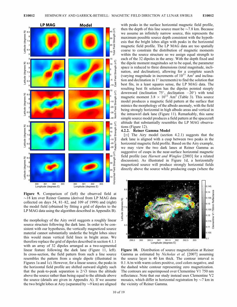
final model dipole grid is magnetized with inclination +4�and declination�12� at a depth of 1.6 km (but again, depth isnot well constrained by the LP MAG data), and has totalmagnetic moment �1.4 � 1013 Am2 distributed as shown inFigure 8. The source model is spatially coarse but is consis-tent with a source structure that is elongated in the east-westdirection and is most intense in the brightest part of thealbedo anomaly. Figure 9 shows that the resulting modelfield compares well with the observed field. For comparison,Nicholas et al. [2007] modeled the Reiner Gamma source asa grid of dipoles separated by 0.1� and placed at the surface,coincident with the albedo anomaly. Those authors assumeda northward magnetization and solved for the magnitude andsign at each of the dipoles, obtaining the distribution ofmagnetization illustrated in Figure 10. In spite of the verydifferent methods employed, the two results resemble oneanother, predicting strong magnetization in the brightest partsof the anomaly.
4.2. Albedo Pattern Matching
[23] The results of the genetic search algorithm sug-gest that the distribution of the underlying source materialcoincides roughly with the shape of the albedo anomaly:a north-south distribution for Airy and an east-west distri-bution for Reiner Gamma. Here, we refine our source modelsby applying the constraint that the near-surface field bestructured according to our hypothesis: strongly horizontalover the brightest parts of swirls and vertical in the intraswirldark lanes. This allows for greatly improved spatial resolu-tion since Clementine reflectance mosaics are availableat 256 pixels/degree whereas LP MAG data are limited to�1–4 pixels/degree. If our hypothesis is correct, sourcemodels constrained by the albedo pattern should producefields that are consistent with the LP MAG observationsmade at higher altitudes. Below, we show that even simplesource models are sufficient to accomplish this, suggestingthat our models are highly plausible.4.2.1. Airy Model[24] Given the downward-pointing magnetization at Airy
(section 4.1.1) and the associated field pattern (Figure 1c),
Figure 8. The Reiner Gamma source model obtained via the genetic search algorithm described insection 4.1.2. (left) Each square represents a single dipole covering 0.25� � 0.25� (roughly 5.7 �107 m2) with the color indicating each dipole’s total magnetic moment (typical values in the center are�3.4 � 1011 Am2 per dipole). (right) The same information as contours over Clementine albedo.
HEMINGWAY AND GARRICK-BETHELL: MAGNETIC FIELD DIRECTION AT LUNAR SWIRLS E10012E10012
9 of 19
the morphology of the Airy swirl suggests a roughly linearsource structure following the dark lane. In order to be con-sistent with our hypothesis, the vertically magnetized sourcematerial cannot substantially underlie the bright lobes sincethis would mean vertical field lines in bright areas. Wetherefore replace the grid of dipoles described in section 4.1.1with an array of 32 dipoles arranged as a two-segmentedlinear feature following the dark lane (Figure 11, left).In cross-section, the field pattern from such a line sourceresembles the pattern from a single dipole (illustrated inFigures 1a and 1c). However, for a linear source, the peaks inthe horizontal field profile are shifted outward slightly suchthat the peak-to-peak separation is 2/√3 times the altitudeabove the source rather than being equal to the altitude abovethe source (details are given in Appendix A). If we assumethe two bright lobes at Airy (separated by�9 km) are aligned
with peaks in the surface horizontal magnetic field profile,then the depth of this line source must be �7.8 km. Becausewe assume an infinitely narrow source, this represents themaximum possible source depth consistent with the hypoth-esis that the bright lobes align with peaks in the horizontalmagnetic field profile. The LP MAG data are too spatiallycoarse to constrain the distribution of magnetic momentswithin the source structure so we assign equal strength toeach of the 32 dipoles in the array. With the depth fixed andthe dipole moment magnitudes set to be equal, the parameterspace is reduced to three dimensions (total magnitude, incli-nation, and declination), allowing for a complete search(varying magnitude in increments of 1011 Am2 and inclina-tion and declination in 1� increments) to find the solution thatbest fits, in a least squares sense, the LP MAG data. Theresulting best fit solution has the dipoles pointed steeplydownward (inclination 75�, declination �20�) with totalmagnetic moment 3.8 � 1012 Am2 (Table 3). This sourcemodel produces a magnetic field pattern at the surface thatmimics the morphology of the albedo anomaly, with the fieldbeing strongly horizontal in high albedo areas and vertical inthe intraswirl dark lane (Figure 11). Remarkably, this samesimple source model produces a field pattern at the spacecraftaltitude that substantially resembles the LP MAG observa-tions (Figure 12).4.2.2. Reiner Gamma Model[25] The Airy model (section 4.2.1) suggests that the
dark lane is aligned with a cusp between two peaks in thehorizontal magnetic field profile. Based on the Airy example,we may view the two dark lanes at Reiner Gamma assuggestive of cusps in the near-surface horizontal magneticfield profile (see Harnett and Winglee [2003] for a relateddiscussion). As illustrated in Figure 1d, a horizontallymagnetized source will produce strongly horizontal fieldsdirectly above the source while producing cusps (where the
Figure 9. Comparison of (left) the observed field at�18 km over Reiner Gamma (derived from LP MAG datacollected on days 54, 81–82, and 109 of 1999) and (right)the model field (obtained by fitting a grid of dipoles to theLP MAG data using the algorithm described in Appendix B).
Figure 10. Distribution of source magnetization at ReinerGamma as estimated by Nicholas et al. [2007] assumingthe source layer is 40 km thick. The contour interval is0.1 A/m with warm colors positive, cool colors negative, andthe dashed white contour representing zero magnetization.The contours are superimposed over Clementine V1 750 nmreflectance. Note that our study instead uses Clementine V2mosaics, which differ in horizontal registration by �7 km inthe vicinity of Reiner Gamma.
HEMINGWAY AND GARRICK-BETHELL: MAGNETIC FIELD DIRECTION AT LUNAR SWIRLS E10012E10012
10 of 19
horizontal field strength drops to zero) on either side of thesource. This suggests that the horizontally magnetized sourcematerial underlies the brightest parts of the Reiner Gammaalbedo feature and that the dark lanes may be aligned with thecusps. The appearance of the two dark lanes and the rela-tively bright material between them may be explained by asuperposition of two sources (see Figure 13 and comparewith Figure 1).[26] As with the case illustrated in Figures 1b and 1d, the
field illustrated in Figure 13 is strongly horizontal at anyaltitude over the two horizontally magnetized sources.However, in this case there is an additional region of elevatedhorizontal field strength where the side lobes interfere con-structively between the two sources. Taking this pattern as acue, we replace the grid of dipoles described in section 4.1.2with an array of 55 dipoles arranged as curvilinear structuresbeneath the three brightest parts of the swirl (Figure 14, left).In cross-section, the field pattern from the two approximatelylinear sources adjacent to the dark lanes resembles the patternfrom the two-dipole case illustrated in Figure 13, but thecusps in the horizontal magnetic field profile are shiftedoutward slightly such that they are displaced laterally (in thiscase to the north and south) from the center of the sourcesby a distance equal to the altitude above the source ratherthan 1/√2 times the altitude above the source (details aregiven in Appendix A). If we assume the dark lanes at ReinerGamma (which are displaced �5 km from the centers of thebright lobes) are aligned with the cusps in the surface hori-zontal magnetic field profile, then the depth of the sourcemust be �5 km. Because we assume infinitely narrow sourcestructures, this represents the maximum possible source depthconsistent with the hypothesis that the dark lanes align withcusps in the horizontal magnetic field profile. The LP MAGdata are too spatially coarse to constrain the distribution ofmagnetic moments within the source structure so we assignequal strength to each of the 55 dipoles in the array. As withthe Airy case, we perform a complete search to find the solu-tion that best fits, in a least squares sense, the LP MAG data.The resulting best fit solution has the dipoles pointed withinclination +2� and declination �8� (i.e., pointed nearly hori-zontally and slightly west of north) and total magnetic moment
1.0 � 1013 Am2 (Table 4). This source model produces amagnetic field pattern at the surface that mimics the mor-phology of the albedo anomaly, with the field being stronglyhorizontal in high albedo areas and vertical in the intraswirl
Figure 11. (left) Airy study area showing Clementine albedo map with red circles indicating the locationsof the source model’s 32 dipoles. (right) Resulting horizontal magnetic field strength predicted at the sur-face. White arrows indicate where field lines become vertical in the intraswirl dark lane. Figure 12 com-pares the model field predicted at the spacecraft altitude with the LP MAG observations.
Table 3. Final Dipole Array Model for Airy as Described inSection 4.2.1a
aSee Figure 11. The model consists of 32 dipoles at the indicated latitudesand longitudes, all buried 7.8 km below the surface. The total magneticmoment is 3.8� 1012 Am2. Inclination is measured positive downward fromthe horizontal and declination is measured positive clockwise from north.
HEMINGWAY AND GARRICK-BETHELL: MAGNETIC FIELD DIRECTION AT LUNAR SWIRLS E10012E10012
11 of 19
dark lanes (Figure 14). Remarkably, this same source modelproduces a field pattern at the spacecraft altitude that agreeswith the Lunar Prospector observations (Figure 15).
5. Discussion
5.1. Magnetization
[27] The models described in section 4.1 suggest that thesource material is concentrated under the central parts of thealbedo anomalies. Based on the source material distributionsillustrated in Figures 6 and 8, we can compute the impliedmagnetizations at Airy and Reiner Gamma for variousassumed layer thicknesses. Figure 16 illustrates that evenwhen the magnetized layer is assumed to be 10 km thick,
typical magnetizations at the Reiner Gamma anomaly are onthe order of 1 A/m. If the magnetized layer is only 1 km thick,the implied magnetization approaches 10 A/m at ReinerGamma. For comparison, Nicholas et al. [2007] predict aminimum magnetization of 1 A/m for a layer 1 km thick atReiner Gamma andWieczorek et al. [2012] calculate�2 A/mfor the same layer thickness assuming an anomaly that pro-duces a 10 nT field at 30 km altitude. If we suppose thesource structures are further horizontally concentrated, asthe albedo-pattern-constrained models of section 4.2 suggest(Figures 11 and 14), the magnetizations would have to beeven greater.
5.2. Magnetizing Field
[28] The strong magnetizations at the Airy and ReinerGamma anomalies could be the result of the source materialhaving cooled in a long lasting global magnetic field, perhapsgenerated by a core dynamo [Garrick-Bethell et al., 2009;
Figure 12. Comparison of (left) the observed field at�18 km over Airy (derived from LP MAG data collectedon days 49–50, 77, and 104 of 1999) and (right) the modelfield (obtained as described in section 4.2.1). Figure 11shows the horizontal component of the model field pre-dicted at the surface.
Figure 13. (top) Magnetic field lines due to a pair of dipolesseparated by 15 km and oriented horizontally in the plane ofthe page. (bottom) Profiles of the horizontal component ofthe magnetic field shown at the various altitudes representedby dashed lines in Figure 13 (top). Each of the dipoles has amagnetic moment of 1012 Am2.
HEMINGWAY AND GARRICK-BETHELL: MAGNETIC FIELD DIRECTION AT LUNAR SWIRLS E10012E10012
12 of 19
Dwyer et al., 2011; Le Bars et al., 2011; Shea et al., 2012].As we have shown here, however, the Airy anomaly (locatedat approximately 17�S, 3�E) is magnetized with a steepdownward inclination while the Reiner Gamma anomaly(located at approximately 7�N, 59�W) is magnetized withalmost zero inclination and points approximately toward thenorth. If these two anomalies acquired their magnetizationsby cooling in a dipolar dynamo field, they could not haveformed contemporaneously. Instead, the two anomalies mayhave formed during different global field orientation epochs.Alternatively, the Moon’s dynamo field may have had sub-stantial higher order components (i.e., beyond dipolar).[29] Another possibility that avoids the difficulties associ-
ated with inconsistent magnetization directions is that, ratherthan being the thermal remanent magnetization signaturesof an extinct core dynamo, the Moon’s crustal magneticanomalies may instead be the result of shock remanentmagnetization that occurs following basin-forming impactevents when magnetohydrodynamic shock waves convergenear the basin antipode producing strong transient fields andpotentially magnetizing iron-rich ejecta materials [Hoodet al., 2001; Halekas et al., 2001; Richmond et al., 2005;Hood and Artemieva, 2008].
6. Conclusions
[30] Our examination of swirls at Airy and Reiner Gamma,two magnetic anomalies with dissimilar orientation, suggeststhat magnetic field direction and swirl morphology arerelated in the way we predict based on the solar winddeflection hypothesis: the Reiner Gamma case delivers evi-dence that swirls are brightest where magnetic field lines aredominantly horizontal and the Airy case demonstrates aconnection between dark lanes and vertically oriented fieldlines. These findings support the solar wind deflection modelfor swirl formation, implying that differential solar winddarkening is largely responsible for creating the albedoanomalies. Although our source models do not representunique solutions, they agree with observational constraintswhile plausibly accounting for the alternating bright and darkbands at both Airy and Reiner Gamma. Our model results
suggest that swirl morphology could potentially be used toinfer small-scale structure in the near-surface magnetic fieldas well as the layout and burial depth of the magnetic sourcematerial. For Airy and Reiner Gamma, we infer maximumsource burial depths of �8 km and �5 km, respectively, andhorizontally concentrated sources with strong magnetizations(�10 A/m or greater for a layer 1 km thick). Examination ofadditional swirls may help to further our understanding ofhow magnetic field direction relates to swirl morphology, butultimately, very near-surface magnetic field and solar windflux measurements (i.e., from altitudes of hundreds of metersor less) will be required to confirm our predictions.
Appendix A: Magnetic Field Profile Calculations
[31] Here, we calculate the locations of the maxima andminima in the horizontal magnetic field profiles due to bothvertically and horizontally magnetized sources. We firstconsider the single dipole sources illustrated in Figure 1 andthen repeat the calculations for the line sources discussed insection 4.
A1. Single Dipole Source
[32] If we take the horizontal and vertical positions inFigures 1a and 1b to be the x and z coordinates, respectively,and if the magnetic dipoles are each located at the origin withmagnitude and orientation represented by a vector, m, thenthe resulting magnetic field,B, at a position, r = (x̂{{{{+ y|̂|||||+ zk̂),is given by:
B ¼ m0
4p3 m ⋅ rð Þr�mr2
� � 1
r5ðA1Þ
Equation (A1) is adapted from Blakely [1995, p. 75]. Here,we employ SI units with m0 being the magnetic permeabilityof free space. For points in the x-z plane, the horizontalcomponent of the magnetic field (Bh) is identical to themagnitude of the x-component (Bx) since, by symmetry,magnetic field lines cannot cross the x-z plane (i.e., cannothave a y-component). Considering the case of the vertically
Figure 14. (left) Reiner Gamma study area showing Clementine albedo map with red circles indicatingthe locations of the source model’s 55 dipoles. (right) Resulting horizontal magnetic field strength predictedat the surface. White arrows indicate where field lines become vertical in one of the intraswirl dark lanes.Figure 15 compares the model field predicted at the spacecraft altitude with the LP MAG observations.
HEMINGWAY AND GARRICK-BETHELL: MAGNETIC FIELD DIRECTION AT LUNAR SWIRLS E10012E10012
13 of 19
oriented dipole (m = [0 0 m]T ), the horizontal componentof the magnetic field becomes:
Bh ¼ Bxj j ¼ m0
4p3mzx
x2 þ z2ð Þ52
( )ðA2Þ
Equation (A2) demonstrates that field lines directly over avertically oriented dipole are vertical at any altitude becauseBh = 0 when x = 0 (this is also evident in Figure 1a).Differentiating equation (A2) with respect to x and settingthe result to zero yields the positions of the peaks in thehorizontal field strength profile:
xBhmax¼ � 1
2z ðA3Þ
This means that the separation between peaks (2x) is equalto the altitude above the source (z), which is evident inFigure 1c.[33] Considering the case of the horizontally oriented
dipole (m = [m 0 0]T ), and still being restricted to points in
Table 4. Final Dipole Array Model for Reiner Gamma asDescribed in Section 4.2.2a
aSee Figure 14. The model consists of 55 dipoles at the indicated latitudesand longitudes, all buried 5 km below the surface. The total magneticmoment is 1.0� 1013 Am2. Inclination is measured positive downward fromthe horizontal and declination is measured positive clockwise from north.
Figure 15. Comparison of (left) the observed field at�18 km over Reiner Gamma (derived from LP MAG datacollected on days 54, 81–82, and 109 of 1999) and (right)the model field (obtained as described in section 4.2.2).Figure 14 shows the horizontal component of the model fieldpredicted at the surface.
HEMINGWAY AND GARRICK-BETHELL: MAGNETIC FIELD DIRECTION AT LUNAR SWIRLS E10012E10012
14 of 19
the x-z plane, the vertical (z) component of the magnetic fieldbecomes:
Bv ¼ Bzj j ¼ m0
4p3mxz
x2 þ z2ð Þ52
( )ðA4Þ
Equation (A4) demonstrates that field lines directly over ahorizontally oriented dipole are horizontal at any altitudebecause Bz = 0 when x = 0 (Figure 1b). Again, starting fromequation (A1), and considering only points in the x-z plane,the horizontal component of the magnetic field due to ahorizontally oriented dipole that is aligned with the x axisbecomes:
Bh ¼ Bxj j ¼ m0
4pm 2x2 � z2ð Þx2 þ z2ð Þ52
( )ðA5Þ
Setting equation (A5) to zero shows that the horizontal fieldstrength drops to zero when:
xBh¼0 ¼ � 1ffiffiffi2
p z ðA6Þ
Hence, the cusps in the horizontal magnetic field profileare laterally displaced from the source by a distance of1/√2 times the altitude above the source (this is evident inFigure 1d).
A2. Linear Source
[34] Imagine that instead of a single dipole, the source is alinear structure such as a long, uniformly magnetized cylin-der. If this linear source is infinitely long and coincident with
the y axis, and the magnetization per unit length is m′, thenthe magnetic field is given by:
B ¼ m0
4p4 m′ ⋅ rð Þr� 2m′r2
� � 1
r4ðA7Þ
Equation (A7) is adapted from Blakely [1995, p. 96]. Again,considering only points in the x-z plane, the horizontalcomponent of the magnetic field due to the vertically mag-netized line source becomes:
Bh ¼ Bxj j ¼ m0
4p4m′zx
x2 þ z2ð Þ2( )
ðA8Þ
As with the dipole case, field lines directly over a verticallymagnetized line source are vertical at any altitude. Differen-tiating equation (A8) with respect to x and setting the result tozero yields the positions of the peaks in the horizontal fieldprofile:
xBhmax¼ � 1ffiffiffi
3p z ðA9Þ
Considering the case of a horizontally magnetized line source,the vertical (z) component of the magnetic field becomes:
Bv ¼ Bzj j ¼ m0
4p4m′xz
x2 þ z2ð Þ2( )
ðA10Þ
Hence, field lines directly over a horizontally magnetizedlinear source are horizontal at any altitude. Again, startingfrom equation (A7), and considering only points in the x-zplane, the horizontal component of the magnetic field due to alinear source coincident with the y axis and magnetizationparallel to the x axis becomes:
Bh ¼ Bxj j ¼ m0
4p2m′ x2 � z2ð Þx2 þ z2ð Þ2
( )ðA11Þ
Setting equation (A11) to zero shows that the horizontal fieldstrength drops to zero when:
xBh¼0 ¼ �z ðA12Þ
Hence, the cusps in the horizontal magnetic field profile arelaterally displaced from the line source by a distance equal tothe altitude above the source.
Appendix B: Genetic Search Algorithm
[35] The magnetic source models discussed in section 4.1were obtained using a heuristic search technique known as
Figure 16. Rock magnetization implied by source modelsillustrated in Figures 6 and 8 versus assumed layer thick-ness. Solid lines are based on the maximum individual dipolemoments found in those models (�2.1 � 1011 Am2 for Airy,�6.5 � 1011 Am2 for Reiner Gamma), and the dashed linesare based on characteristic values of 1.25 � 1011 Am2 forAiry and 3.4 � 1011 Am2 for Reiner Gamma.
Table B1. The 211 ‘Genes’ That Define an Individual SourceModel
Gene Number Controls
1 Dipole grid burial depth (km)2 Magnetic moment inclination (deg)3 Magnetic moment declination (deg)4 Magnitude of dipole #1 (Am2)… …211 Magnitude of dipole #208 (Am2)
HEMINGWAY AND GARRICK-BETHELL: MAGNETIC FIELD DIRECTION AT LUNAR SWIRLS E10012E10012
15 of 19
Figure B1. Snapshots at generations 1, 100, 300, and 600 during the evolution of the dipole grid sourcemodels for (left) Airy and (right) Reiner Gamma. Each panel shows the distribution of magnetic momentsfrom the best-performing model of the specified generation.
HEMINGWAY AND GARRICK-BETHELL: MAGNETIC FIELD DIRECTION AT LUNAR SWIRLS E10012E10012
16 of 19
a genetic algorithm. Genetic algorithms have a diverse rangeof applications [Holland, 1992; Goldberg, 1989] includinglarge-scale optimization problems such as ours: to find asource model (defined by 211 parameters) that producesminimal error between predicted and observed magneticfields. Genetic algorithms employ concepts borrowed fromgene-centered biological evolution [Dawkins, 1976] in orderto iteratively (i.e., over many generations) progress towardsolutions with increasing degrees of ‘fitness’. In our case, this‘fitness’ is a measure of how well the magnetic field pro-duced by the source model matches the Lunar Prospectormagnetometer (LP MAG) observations.[36] Our algorithm begins by generating a population of
individual source models with randomly distributed char-acteristics. The characteristics of each individual sourcemodel are defined by its ‘genes’, with each individual havingthe 211 distinct genes listed in Table B1. At each iteration, orgeneration, the individual members of the population areevaluated according to how well they predict the magneticfield at each of the LPMAG observation points. We computethe error between the prediction and the observation using the‘effective error’ metric described in section 4.1.1. We thenrank the individuals from lowest to highest sum of squaredeffective errors. The individuals with the lowest errors arethen selected as the ‘parents’ of the next generation. The nextiteration begins by generating a new population to replace theprevious generation. Each individual in the new generationis formed by setting each of its 211 genes equal to thecorresponding gene from one of its parents in a processknown as crossover (analogous to chromosomal crossover).For example, an individual’s gene for inclination will matchthe inclination gene of one of its parents (chosen at randomfrom among the parents). Because only the best-performingindividuals contribute their genes to the next generation,individuals of each new generation tend to inherit the bestcharacteristics of the previous generation. We then applyrandom mutations (i.e., randomly adjust several isolated
genes). This step ensures variation in the population andallows for the possibility of introducing advantageous genesnot possessed by the parents. Finally, members of the newgeneration are evaluated and their best performers areselected as the parents of the next generation. With eachgeneration, genes that result in large model errors tend to bediscarded while genes that result in smaller model errors tendto be retained. Inheritance and selection lead the gene pool tobe increasingly rich in genes that form good source modelswhile crossover and mutations ensure variation, allowingfor innovations that can lead offspring to outperform theirparents. The result is that the population progresses graduallytoward optimality in terms of minimum model error.[37] While this explanation captures the essence of the
algorithm, our implementation includes additional detailssuch as gene mutation rate (the probability that any givengene will mutate) and how “random” mutations are distrib-uted (i.e., it is not useful to have sudden changes in burialdepth on the order of 1000 km, for example, so mutationsmust be limited to reasonable adjustments according to somedistribution). We experimented with various population sizesand numbers of parents selected at each generation (theremust be at least two parents but more than two is alsoallowed). For computational efficiency, a small populationsize is preferred. The algorithm was found to operate effec-tively with a population of just 10 individuals in which thetop-performing 3 contribute their genes to the next genera-tion. We allow mutations to occur with a probability of0.1 and when they do occur, the gene is adjusted from itscurrent value according to a normal distribution with somepre-defined standard deviation (which depends on whetherthe gene has units of kilometers, degrees or Am2). We alsoapply smaller mutations with a higher probability in order toensure a measurable degree of variation in the population.The initial population is generated based on a seed model;each individual in the initial population is formed by apply-ing normally distributed adjustments to each of the genes in
Figure B2. Evolution of dipole grid source model error over 600 generations for (left) Airy and(right) Reiner Gamma. The error shown is the sum of squared ‘effective’ errors (as described insection 4.1.1) over all LP MAG data points for the best-performing model in each generation.
HEMINGWAY AND GARRICK-BETHELL: MAGNETIC FIELD DIRECTION AT LUNAR SWIRLS E10012E10012
17 of 19
the seed model. While the choice of seed model and param-eter settings influences the efficiency of the algorithm (i.e.,how quickly it reaches a good solution), the end results tendto be very similar across a wide range of parameters andinitial conditions. For the dipole grid source models pre-sented in section 4.1, the algorithm was allowed to iteratethrough 600 generations (Figure B1). Based on the trends inerror evolution (Figure B2), we would not expect additionaliterations to yield substantial improvements.
[38] Acknowledgments. This research was performed as part of theWorld Class University Project at Kyung Hee University and sponsoredby the Korean Ministry of Education, Science and Technology. Additionalsupport was provided by the NASA Ames Research Center/University ofCalifornia Santa Cruz University Affiliated Research Center. We would liketo thank Lon Hood, Robert Lin, Jasper Halekas, Greg Delory, Robert Lillis,and Michael Purucker for their comments and suggestions and JosephNicholas for the data used to generate Figure 10.
ReferencesArchinal, B. B. A., M. R. Rosiek, R. L. Kirk, and B. L. Redding (2006), TheUnified Lunar Control Network 2005, U.S. Geol. Surv. Open File Rep.,2006-1367.
Blakely, R. J. (1995), Potential Theory in Gravity and Magnetic Applica-tions, Cambridge Univ. Press, Cambridge, U. K., doi:10.1017/CBO9780511549816.
Blewett, D. T., B. R. Hawke, N. C. Richmond, and C. G. Hughes(2007), A magnetic anomaly associated with an albedo feature near Airycrater in the lunar nearside highlands, Geophys. Res. Lett., 34, L24206,doi:10.1029/2007GL031670.
Blewett, D. T., E. I. Coman, B. R. Hawke, J. J. Gillis-Davis, M. E.Purucker, and C. G. Hughes (2011), Lunar swirls: Examining crustalmagnetic anomalies and space weathering trends, J. Geophys. Res.,116, E02002, doi:10.1029/2010JE003656.
Coleman, P. J., B. R. Lichtenstein, C. T. Russell, L. R. Sharp, andG. Schubert (1972), Magnetic fields near the moon, Proc. Lunar Sci.Conf., 3rd, 2271–2286.
Dawkins, R. (1976), The Selfish Gene, Oxford Univ. Press, Oxford, U. K.Dwyer, C. A., D. J. Stevenson, and F. Nimmo (2011), A long-lived lunardynamo driven by continuous mechanical stirring, Nature, 479(7372),212–214, doi:10.1038/nature10564.
Dyal, P., C. W. Parkin, and C. P. Sonett (1970), Apollo 12 Magnetometer:Measurement of a steady magnetic field on the surface of the Moon,Science, 169(3947), 762–764, doi:10.1126/science.169.3947.762.
Dyment, J., and J. Arkani-Hamed (1998), Equivalent source magneticdipoles revisited, Geophys. Res. Lett., 25(11), 2003–2006, doi:10.1029/98GL51331.
Garrick-Bethell, I., B. P. Weiss, D. L. Shuster, and J. Buz (2009),Early lunar magnetism, Science, 323(5912), 356–359, doi:10.1126/science.1166804.
Garrick-Bethell, I., J. W. Head, and C. M. Pieters (2011), Spectral proper-ties, magnetic fields, and dust transport at lunar swirls, Icarus, 212(2),480–492, doi:10.1016/j.icarus.2010.11.036.
Goldberg, D. (1989), Genetic Algorithms in Search, Optimization andMachine Learning, Addison-Wesley, Reading, Mass.
Halekas, J. S., D. L. Mitchell, R. P. Lin, S. Frey, L. L. Hood, M. H. Acuña,and A. B. Binder (2001), Mapping of crustal magnetic anomalies on thelunar near side by the Lunar Prospector electron reflectometer, J. Geophys.Res., 106(E11), 27,841–27,852, doi:10.1029/2000JE001380.
Hapke, B. (2001), Space weathering from Mercury to the asteroid belt,J. Geophys. Res., 106(E5), 10,039–10,073, doi:10.1029/2000JE001338.
Harnett, E. M., and R. M. Winglee (2003), 2.5-D fluid simulations of thesolar wind interacting with multiple dipoles on the surface of the Moon,J. Geophys. Res., 108(A2), 1088, doi:10.1029/2002JA009617.
Holland, J. (1992), Adaptation in Natural and Artificial Systems: An Intro-ductory Analysis with Applications to Biology, Control, and ArtificialIntelligence, MIT Press, Cambridge, Mass.
Hood, L. L. (2011), Central magnetic anomalies of Nectarian-aged lunarimpact basins: Probable evidence for an early core dynamo, Icarus,211(2), 1109–1128, doi:10.1016/j.icarus.2010.08.012.
Hood, L. L., and N. A. Artemieva (2008), Antipodal effects of lunar basin-forming impacts: Initial 3D simulations and comparisons with observa-tions, Icarus, 193(2), 485–502, doi:10.1016/j.icarus.2007.08.023.
Hood, L. L., and G. Schubert (1980), lunar magnetic anomalies and surfaceoptical properties, Science, 208, 49–51, doi:10.1126/science.208.4439.49.
Hood, L. L., and C. R. Williams (1989), The lunar swirls: Distribution andpossible origins, Proc. Lunar Planet. Sci. Conf., 19th, 99–113.
Hood, L. L., P. J. Coleman, and D. E. Wilhelms (1979), Lunar nearsidemagnetic anomalies, in Proc. Lunar Planet. Sci. Conf., 10th, 2235–2257.
Hood, L. L., C. T. Russell, and P. Coleman (1981), Contour maps of lunarremanent magnetic fields, J. Geophys. Res., 86, 1055–1069, doi:10.1029/JB086iB02p01055.
Hood, L. L., A. Zakharian, J. Halekas, D. L. Mitchell, R. P. Lin, M. H.Acuña, and A. B. Binder (2001), Initial mapping and interpretation of lunarcrustal magnetic anomalies using Lunar Prospector magnetometer data,J. Geophys. Res., 106(E11), 27,825–27,839, doi:10.1029/2000JE001366.
Kramer, G. Y., et al. (2011), M3 spectral analysis of lunar swirls and the linkbetween optical maturation and surface hydroxyl formation at magneticanomalies, J. Geophys. Res., 116, E00G18, doi:10.1029/2010JE003729.
Kurata, M., H. Tsunakawa, Y. Saito, H. Shibuya, M. Matsushima, andH. Shimizu (2005), Mini-magnetosphere over the Reiner Gamma mag-netic anomaly region on the Moon, Geophys. Res. Lett., 32, L24205,doi:10.1029/2005GL024097.
Le Bars, M., M. A. Wieczorek, Ö. Karatekin, D. Cébron, and M. Laneuville(2011), An impact-driven dynamo for the early Moon, Nature,479(7372), 215–218, doi:10.1038/nature10565.
Lin, R. P. (1979), Constraints on the origins of lunar magnetism from elec-tron reflection measurements of surface magnetic fields, Phys. EarthPlanet. Inter., 20, 271–280, doi:10.1016/0031-9201(79)90050-5.
Lin, R. P., D. L. Mitchell, D. W. Curtis, K. A. Anderson, C. W. Carlson,J. McFadden, M. H. Acuña, L. L. Hood, and A. Binder (1998), Lunar sur-face magnetic fields and their interaction with the solar wind: Resultsfrom lunar prospector, Science, 281(5382), 1480–1484, doi:10.1126/science.281.5382.1480.
Neish, C. D., D. T. Blewett, D. B. J. Bussey, S. J. Lawrence, M. Mechtley,and B. J. Thomson (2011), The surficial nature of lunar swirls as revealedby the Mini-RF instrument, Icarus, 215(1), 186–196, doi:10.1016/j.icarus.2011.06.037.
Ness, N. F., K. W. Behannon, C. S. Scearce, and S. C. Cantarano (1967),Early results from the magnetic field experiment on Lunar Explorer 35,J. Geophys. Res., 72(23), 5769–5778, doi:10.1029/JZ072i023p05769.
Nicholas, J. B., M. E. Purucker, and T. J. Sabaka (2007), Age spot or youth-ful marking: Origin of Reiner Gamma, Geophys. Res. Lett., 34, L02205,doi:10.1029/2006GL027794.
Parker, R. L. (2003), Ideal bodies for Mars magnetics, J. Geophys. Res.,108(E1), 5006, doi:10.1029/2001JE001760.
Pieters, C. M., et al. (2009), Character and spatial distribution of OH/H2Oon the surface of the Moon seen by M3 on Chandrayaan-1, Science,326(5952), 568–572, doi:10.1126/science.1178658.
Pinet, P. C., V. V. Shevchenko, S. D. Chevrel, Y. Daydou, and C. Rosemberg(2000), Local and regional lunar regolith characteristics at Reiner GammaFormation: Optical and spectroscopic properties from Clementine andEarth-based data, J. Geophys. Res., 105(E4), 9457–9475, doi:10.1029/1999JE001086.
Purucker, M. (2008), A global model of the internal magnetic field of theMoon based on Lunar Prospector magnetometer observations, Icarus,197(1), 19–23, doi:10.1016/j.icarus.2008.03.016.
Purucker, M. E., and J. B. Nicholas (2010), Global spherical harmonic mod-els of the internal magnetic field of the Moon based on sequential andcoestimation approaches, J. Geophys. Res., 115, E12007, doi:10.1029/2010JE003650.
Purucker, M. E., T. J. Sabaka, and R. A. Langel (1996), Conjugate gradientanalysis: A new tool for studying satellite magnetic data sets, Geophys.Res. Lett., 23(5), 507–510, doi:10.1029/96GL00388.
Richmond, N. C., L. L. Hood, D. L. Mitchell, R. P. Lin, M. H. Acuña, andA. B. Binder (2005), Correlations between magnetic anomalies and sur-face geology antipodal to lunar impact basins, J. Geophys. Res., 110,E05011, doi:10.1029/2005JE002405.
Schultz, P. H., and L. J. Srnka (1980), Cometary collisions on the Moon andMercury, Nature, 284, 22–26, doi:10.1038/284022a0.
Shea, E. K., B. P. Weiss, W. S. Cassata, D. L. Shuster, S. M. Tikoo,J. Gattacceca, T. L. Grove, and M. D. Fuller (2012), A long-lived lunar coredynamo, Science, 335(6067), 453–456, doi:10.1126/science.1215359.
Shibuya, H., H. Tsunakawa, F. Takahashi, H. Shimizu, and M. Matsushima(2010), Near surface magnetic field mapping over the swirls in theSPA region using Kaguya LMAG data, EPSC Abstr., 5, AbstractEPSC2010-166.
Smith, D. E., et al. (2010), Initial observations from the Lunar Orbiter LaserAltimeter (LOLA), Geophys. Res. Lett., 37, L18204, doi:10.1029/2010GL043751.
Starukhina, L. V., and Y. G. Shkuratov (2004), Swirls on the Moon andMercury: Meteoroid swarm encounters as a formation mechanism, Icarus,167(1), 136–147, doi:10.1016/j.icarus.2003.08.022.
HEMINGWAY AND GARRICK-BETHELL: MAGNETIC FIELD DIRECTION AT LUNAR SWIRLS E10012E10012
18 of 19
Vernazza, P., R. P. Binzel, A. Rossi, M. Fulchignoni, and M. Birlan (2009),Solar wind as the origin of rapid reddening of asteroid surfaces, Nature,458(7241), 993–995, doi:10.1038/nature07956.
Von Frese, R. R. B., W. J. Hinze, and L. W. Braile (1981), Spherical Earthgravity and magnetic anomaly analysis by equivalent point source inversion,Earth Planet. Sci. Lett., 53, 69–83, doi:10.1016/0012-821X(81)90027-3.
Wieczorek, M. A., B. P. Weiss, and S. T. Stewart (2012), An impactororigin for lunar magnetic anomalies, Science, 335(6073), 1212–1215,doi:10.1126/science.1214773.
HEMINGWAY AND GARRICK-BETHELL: MAGNETIC FIELD DIRECTION AT LUNAR SWIRLS E10012E10012