NeuroImage 13, 856–876 (2001)doi:10.1006/nimg.2000.0730, available online at http://www.idealibrary.com on
Magnetic Resonance Image Tissue Classification Usinga Partial Volume Model
David W. Shattuck,* Stephanie R. Sandor-Leahy,† Kirt A. Schaper,‡David A. Rottenberg,‡,§ and Richard M. Leahy*
*Signal and Image Processing Institute, University of Southern California, Los Angeles, California 90089; †TRW, Inc., Redondo Beach,California 90278; ‡PET Imaging Center, VA Medical Center, Minneapolis, Minnesota 55417; and §Department of Neurology and
Department of Radiology, University of Minnesota, Minneapolis, Minnesota 55455
Accurate classification of magnetic resonance imagesaccording to tissue type at the voxel level is importantin many neuroimaging applications. Changes in thecomposition of gray matter (GM), white matter (WM),or cerebrospinal fluid (CSF) in the whole volume or
within specific regions can be used to characterizephysiological processes and disease entities (Guttmannet al., 1998) or to characterize disease severity (Heindelet al., 1994). Additionally, fractional content imagescan be used to correct for effects of cerebral atrophy inquantitative PET and MR spectroscopy image volumes(Koepp et al., 1997; Ibanez et al., 1998). Low-level tis-sue classifications also provide anatomical informationabout structures such as the cortical surface, which isuseful for visualization and analysis of neuroimagingdata (Thompson et al., 1998) and as a constraint forocalizing functional activation from magnetoencepha-ography and electroencephalography data (Dale andereno, 1993; Baillet et al., 1999). While MRI can pro-ide relatively high-resolution neuroanatomical de-ails, the identification of tissue information is hin-ered by several factors. These include measurementoise, partial volume effects, and image nonuniformityue to magnetic field inhomogeneities. These artifactsonfound characterization of tissue types based solelyn individual voxel intensities.The problem of segmenting MRI has been exten-
ively addressed by many researchers. A common ap-roach to structural segmentation is the use of atlasegistration-based techniques such as those of Bajcsyt al. (1983), Bajcsy and Kovacic (1989), Miller et al.1993), Christensen et al. (1996), Christensen (1999),nd Davatzikos (1997). In these methods a prelabeledtlas volume is matched to a subject volume. Onceegistration is achieved, the labels are transfered tohe subject and structures in the subject volume aredentified. While these techniques can provide veryood matches with subcortical structures, they do notypically match the cortex well due to intersubject vari-bility of cortical sulci and gyri. These methods canlso be very computationally intensive. Atlas-basedegmentation techniques have been combined withow-level tissue classification by Collins et al., (1999)reatly improving tissue classification rates in the cor-ex.
altae
twcStd(w(pmlbu(tudgsof(
svvtmtavtifib
twut(botca1ngfimn
857MRI TISSUE CLASSIFICATION
In contrast to atlas-based approaches are low-leveltechniques in which the tissue content of each individ-ual voxel in the image is identified. A variety of meth-ods have been developed for low-level tissue classifica-tion, most of which are focused on one or more of thethree tasks addressed in this paper. The first task isskull stripping, in which nonbrain tissue is removedfrom the MRI. The second task is compensation forimage nonuniformity. The third task is the actual la-beling of the individual voxels.
In this paper we present a three-stage method thataddresses the problem of isolating the brain from thecalvarium in T1-weighted MRI and classifying its tis-sues. The stages of the method have been developed tobe minimally interactive and operate in reasonabletime on widely available desktop computer hardware.We begin by applying a skull-stripping routine thatuses anisotropic diffusion filtering, edge detection, andmathematical morphology. We then compensate fornonuniformity in the stripped brain using a methodthat fits a tricubic B-spline to local estimates of imagegain variation. The local estimates are computed byfitting a partial volume tissue measurement model tohistograms of local regions of the image. The measure-ment model uses mean tissue intensity and noise vari-ance values computed from the global image and amultiplicative bias parameter that is estimated foreach region during the histogram fit. Each voxel in theintensity-normalized image is then labeled using amaximum a posteriori (MAP) classifier that combinesthe tissue measurement model with a Gibbs prior thatmodels the spatial properties of brain tissue. We vali-date each stage of our approach using real and phan-tom MRI data. We first review the related literature oneach of the three steps in our algorithm.
Skull Stripping
The first task we address is the analysis of the MRIvolume to identify brain and nonbrain voxels. Ourwork is concerned with the predominant tissues of thebrain: GM, WM, and CSF. The measured signal inten-sities of these tissues can overlap with those of othertissues in the head, such as skin, bone, muscle, fat, anddura. This complicates reliable identification of tissueregions and properties. The difficulties faced by laterstages in our method are lessened by clearly identify-ing what is brain tissue and what is not.
Skull stripping is often performed using a se-quence of mathematical morphological operationsfollowing an initial separation of the brain fromother tissues of the head. Bomans et al. (1990) apply
Marr-Hildreth edge detector, followed by manualabeling of connected components within each slice ofhe volume and a morphological closing operationpplied to improve the surface definition. Brummert al. (1993) segment each slice of the brain using
hresholds determined from estimated gray andhite matter intensities, followed by a sequence of
onnected component and morphology operations.andor and Leahy address the task of brain extrac-ion using anisotropic diffusion filtering, Marr-Hil-reth edge detection, and morphological operationsSandor, 1994; Sandor and Leahy, 1997); the methode use is a refinement of this procedure. Kapur et al.
1996) use an initial classification found by the ex-ectation-maximization (E-M)-based classificationethod by Wells et al. (1996) described below, fol-
owed by morphological processing to isolate therain. This extraction is then refined if necessarysing a deformable surface. Kruggel and von Cramon1999) have produced a “brain peeling” procedurehat performs an initial Lee filtering to smooth non-niformities, followed by a brain delineation proce-ure that combines distance-transforms and edgeradients and finally a sequence of morphologicalteps to clean the initial brain mask. Other examplesf skull stripping techniques include the use of de-ormable templates, as described by Dale et al.1999).
Image Nonuniformity
In an ideal MRI acquisition system, the signal inten-ity measured at each voxel will vary through-out theolume depending only on the tissues present at thatoxel location. In practice, MRI exhibits nonuniformissue intensities caused by inhomogeneities in theagnetic fields, magnetic susceptibility variations in
he subject, and other factors (Sled and Pike, 1998). Asresult, tissue labels cannot be reliably assigned to
oxels based solely on individual voxel intensity. For-unately, nonuniformity in MRI is typically character-zed by a slowly varying gain field, also called a biaseld (Wells et al., 1996), and several methods haveeen developed to compensate for this artifact.Nonuniformity correction is often applied prior to
issue classification. Dawant et al. (1993) identifyhite matter reference points within the MRI vol-me and normalize the image intensities relative tohese; a similar technique is used by Dale et al.1999). DeCarli et al. (1996) compute the differenceetween local median and global median values inrder to estimate intensity variation. Techniqueshat perform bias correction prior to tissue classifi-ation also include homomorphic unsharp maskingnd other filtering techniques (Brinkmann et al.,998). Sled et al. (1998) address the problem ofonuniformity using an approach that estimates aain field to sharpen the histogram of the MRI; thiseld is kept smooth using a cubic B-spline. Thisethod has been publicly released under the nameonparametric nonuniform intensity normalization
osfiioa(tebp(aadKieaBdPfta
aivndwidrtwwa
iacm
emBftmvetpeptwamambmpfaYGLpwmpcpp
vflc(L
(hTZcrtc
t
858 SHATTUCK ET AL.
(N3) (available from http://www.bic.mni.mcgill.ca/software/N3/).
A number of iterative methods correct for nonunifor-mity by alternating between tissue classification andnonuniformity estimation. Wells et al. (1996) devel-ped an E-M-based method in which they perform atatistical classification of the image, then low-passlter the residual difference between a reconstructed
mage and the measured image to provide an estimatef the image bias. This bias is removed from the imagend the process is repeated. Guillemaud and Brady1997) take a similar approach using an additionalissue class and report improved results. Van Leemputt al. (1999a) use the same classification step as Wells,ut estimate the bias field by fitting a fourth-orderolynomial to the bias field residual. Yan and Karp1995) account for the inhomogeneity by incorporating
cubic B-spline into a MAP classifier. MAP labelingpproaches combined with bias estimation are alsoescribed by Nocera and Gee (1997) and Rajapakse andruggel (1998). In each of these iterative methods an
nitial MAP classification is used to reconstruct anstimated image, and the residual between this imagend the measured image is smoothed using a tricubic-spline to represent the nonuniformity; this proce-ure is then iterated. In a similar manner, Pham andrince (1999) incorporate a gain field into an adaptive
uzzy C-means algorithm to produce a spatially adap-ive method for classification that compensates for im-ge nonuniformity.
Tissue Labeling
We define tissue classification to be the process ofssigning a label to each voxel in the volume thatdentifies what types of tissues are present in thatoxel. In addition to measurement noise and imageonuniformity, the classification task is made moreifficult by the finite resolution of the scanning hard-are. In a high-resolution anatomical MRI, the image
s sampled at a spacing on the order of 1 mm in eachimension. The complexity of anatomical structuresesults in numerous voxels that contain multiple tissueypes. The intensity measured at such a voxel will be aeighted average of the intensities of the tissuesithin it; this effect is known as partial volume aver-ging.Mensuration of brain tissue volumes with model-
ng for partial volume effects is useful for PET met-bolic and ligand–receptor studies. Early work onomputing tissue proportions in X-ray computed to-ography appears in Thaler et al. (1978). Choi et al.
(1991) developed a generalized partial volume modelin the form of a Markov random field allowing anynumber of tissues and independent measurements.Rusinek et al. (1991) developed a partial volume
stimation method for two-channel MR measure-ents obtained using specialized pulse sequences.onar et al. (1993) used graphical analysis of the 2-D
eature space formed by two-channel measurementso assign tissue proportions in a three-compartmentodel. Santago and Gage (1993) developed a partial
olume model for analyzing the tissue content of anntire volume to determine relative tissue contribu-ion. Laidlaw et al. (1998) classified MRI using thisartial volume model, adjusting it to a region aboutach voxel to identify the fractional content of thatarticular voxel. Warfield et al. (1999) developed aechnique focused on fractional segmentation ofhite matter into damaged and nondamaged tissue,fter preprocessing by the nonuniformity correctionethod described in Wells et al. (1996) and the use ofspatial template for initial white matter and grayatter segmentation. Numerous algorithms have
een described that use Gibbs priors as statisticalodels for the labeled brain volume. Labeling is
erformed by combining the prior with a likelihoodor the data conditioned on the labels and computingMAP estimate (Leahy et al., 1991; Choi et al., 1991;an and Karp, 1995; Kapur et al., 1996; Nocera andee, 1997; Rajapakse and Kruggel, 1998; Vaneemput et al., 1999b). Pham and Prince (1999)roposed an adaptive fuzzy C-means method inhich the tissue fraction at each voxel is theembership function for that voxel belonging to a
articular class. This is one of several statisticallassification and segmentation techniques that com-ensate for nonuniformity during the classificationrocess (Yan and Karp, 1995; Wells et al., 1996;
Nocera and Gee, 1997; Guillemaud and Brady, 1997;Van Leemput et al., 1999b, as described in the pre-
ious section. There are also numerous techniquesor associating voxels with tissue classes that involveabeling without an inhomogeneity correction, in-luding methods based on neural-network modelsOzkan et al., 1993) and graph theoretics (Wu andeahy, 1991).The tissue classification method used by Dale et al.
1999) is intended for identifying the cerebral cortex,ence only white matter tissue voxels are identified.he cortical surface identification approach ofeng et al. (1999) uses a level-set method to findoupled surfaces representing the interior and exte-ior boundary of the cerebral cortex. Neither ofhese methods labels areas of the brain other thanortex.
METHODS
Skull Stripping
The tissue model we use for nonuniformity estima-ion and voxel classification allows for CSF, GM, and
dvrE(vcb
dstisMie
w
859MRI TISSUE CLASSIFICATION
WM. Our classification problem is greatly simplified ifwe strip skull and scalp tissue from the MRI volumeprior to nonuniformity correction and tissue classifica-tion. Skull stripping is also a useful preprocessing toolfor image registration techniques such as AIR (Woodset al., 1998). Our procedure consists of three steps.First, the MRI is processed with an anisotropic diffu-sion filter to smooth nonessential gradients. We thenapply a Marr–Hildreth edge detector to the filteredimage to identify important anatomical boundaries.The objects defined by these boundaries are identifiedand refined using a sequence of morphological andconnected component operations.
Anisotropic Diffusion Filtering
Our method finds anatomical boundaries that sepa-rate the brain from the dura, skull, and other tissues.In some cases, particularly with MRI data that havelow signal-to-noise ratios, these boundaries will be ob-scured by noise, or their edges will be indistinguishablefrom other edges in the image. For this reason we applyan anisotropic diffusion filter that smoothes noisy re-gions in the image while respecting edge boundaries.
Anisotropic diffusion filtering was proposed as animage processing method by Perona and Malik (1990).Gerig et al. (1992) applied this 2-D technique to slicesof MRI data; it has also been extended to 3-D (Mack-iewich, 1995). The filtered image is modeled as thesolution to the anisotropic diffusion equation
I
t5 ¹z~c~p, t!¹I! 5 c~p, t!¹2I 1 ¹c z ¹I, (1)
where p is a point in R3, ¹ and ¹2 represent the gra-ient and Laplacian operators with respect to spatialariables, and ¹z indicates the divergence operator (Pe-ona and Malik, 1990). If c has a constant value, thenq. (1) is simply the isotropic heat diffusion equation
John, 1982) whose solution is the original image con-olved with a Gaussian kernel with variance that in-reases linearly with time. This convolution will bluroth strong and weak edges.Instead of this, Perona and Malik proposed the use of
iffusion coefficients based on a measure of edgetrength. The diffusion coefficient c(p, t) then adap-ively controls the diffusion strength, smoothing themage within a moderately continuous region while notmoothing across sharp discontinuities. Perona andalik demonstrated that using the gradient of image
ntensity as an estimate of edge strength producesxcellent results. We use the function
c~p, t! 5 g~i¹I~p, t!i! 5 e2i¹I~p,t!i 2/k d2, (2)
here kd is the diffusion constant. Using Eq. (2) givespreference to high-contrast edges over low-contrast
ones. The diffusion Eq. (1) is discretized onto a 3-Dlattice resulting in an update equation for each voxel inthe image,
i k~n11! 5 i k
~n! 1 t0 Oj[Nk
c~ j, n!~i r~j, k!~n! 2 i k
~n!!, (3)
where k is a 3-D spatial index, Nk is the set of 6neighbors nearest k, ik
n is the intensity of the voxelindexed by k at the nth time step, r( j, k) is the voxeladjacent to k opposite j, and t0 is the size of the timestep used to discretize the system. To ensure stability,t0 is selected to be 0 # t0 # 1
7 (Mackiewich, 1995); weuse a time step of 1
8. All intensity values in the volumeare updated at each iteration.
We use two parameters to specify the anisotropicdiffusion filter used in our skull stripping technique.The first is the diffusion parameter, kd, and the secondis the number of iterations, possibly none, applied tothe image. Selection of these parameters is done em-pirically, though in practice we have found that a sin-gle set of parameter settings can often be found for aspecific MRI acquisition system and protocol.
Edge Detection
We locate the anatomical boundaries in MRI brainvolumes using the Marr–Hildreth edge detector (Marrand Hildreth, 1980). This detector has a low computa-tional cost and produces closed contours. Other edgefinding approaches, such as the Canny and Derichemethod (Deriche, 1987), could also be used to produceedge segments from the image. However, in certainregions these segments may be too dense to be formedinto anatomical boundaries using a simple edge linkingprocedure.
The Marr-Hildreth edge detector is based on a low-pass filtering step with a symmetric Gaussian kernel,followed by the localization of zero-crossings in theLaplacian of the filtered image. The Marr–Hildrethoperator, extended to three dimensions, is defined as
C~k! 5 ¹ 2~I~k!pgs~p!!, (4)
where C is the output contour image, I is an inputimage, *is the convolution operator, gs is a Gaussiankernel with variance s2,
gs~p! 51
Î2p se2 i pi 2/2s 2, (5)
p is a point in the 3-D volume, and ¹2 is the Laplacianoperator (Bomans et al., 1990). By finding the voxels inthe contour image, C, where zero-crossings occur, abinary image E is produced that separates the imageinto edge-differentiated segments. The s parameter in
wS
860 SHATTUCK ET AL.
Eq. (5) provides the third parameter for the algorithm.Increasing the value of s makes the blurring kernel
ider, and only very strong edges remain in the image.mall values for s produce narrow filters, resulting in
more edges in the image.Using the Laplacian as opposed to the second deriv-
ative in the direction of the gradient implies the well-known poor localization performance of this detectorfor rounded edges with large curvature. Spurious edgesmay also appear with the Marr–Hildreth operator dueto the closed nature of zero-crossing contours.
We have found that at a resolution appropriate forextracting the brain surface, this processor may detectsulcal boundaries corresponding to white–gray mattertransitions rather than gray–CSF transitions; similar
FIG. 1. Skull-stripping stages. (a) A slice from the initial volumewith diffusion parameter 15). (c) The edge map following applicationfrom the extracted brain, following morphological processing of the
results are described in Bomans et al. (1990). Thus, thecortical surface that we extract during edge detectionhas a tendency to move between the outer corticalboundary on the gyri and the inner cortical surface inthe sulcal folds. This may be overcome during morpho-logical processing.
Morphological Processing
The edge detection step produces a binary volumeE(k), where k is a 3-D spatial index describing a pointin Z3, the 3-D integer space. E(k) represents edge vox-els by values of 0 while nonedge voxels are representedby values of 1; an example image is shown in Fig. 1c, inwhich edge voxels are black and nonedge voxels are
) The same slice after anisotropic diffusion filtering (three iterationshe Marr–Hildreth operator (edge kernel s 5 0.6). (d) The same slicee map.
. (bof tedg
tvlaHlc
s
861MRI TISSUE CLASSIFICATION
white. We denote the set of all nonedge voxels as X 5{xk: E(k) 5 1}. The task of the morphological processoris to select the voxels corresponding to the brain tissuefrom the original image based on the voxels in X.
The edge detector will produce a distinct boundarybetween the brain and the surrounding tissues in mostareas of the MRI volume. The brain should be wellseparated from the rest of the cerebral tissue by edgevoxels in E(k). However, there are often meninges andblood vessels that are not distinguished from the braindue to noise, low contrast between brain and meninges,or true anatomical continuity. The set X will mostlikely contain voxels that link brain regions to extra-neous surrounding structures, such as dura or skin.Fortunately, the connective tissues are characteristi-cally thin with typical widths of 2 mm or less. Connec-tions of this nature are broken by performing a mor-phological erosion on X using a rhombus structuringelement of size 1, which is a 3-D cross with a width of3 voxels. The first morphological step in the algorithmis described by
XE 5 X * R1, (6)
where X is the input edge set, XE is the eroded volume,C is the erosion operator, and R1 is the size 1 rhombusstructuring element. This operation will delete narrowconnections without globally damaging or distortingthe image. For MRI resolutions on the order of 1 mm,regions with a width of 2 mm in any direction will bedeleted.
The eroded set XE will consist of several connectedcomponents. In this context, we use connectedness inthe 6-neighbor sense, in which two voxels are con-nected if and only if they share a common face. Theerosion step Eq. (6) will eliminate a number of smallstructures in the volume and provide increased sepa-ration of larger anatomical structures. We assume thatupon completion of this step the largest connected re-gion centered in the volume consists entirely of braintissue. Additional tests on the mean intensity of con-nected component regions in the MRI volume helpensure that we select the brain and not the back-ground. At this point in the algorithm, a human oper-ator can also intercede should the algorithm select thewrong connected component. We assume that the se-lected region contains nearly all of the brain voxels. Wedescribe the selection step as
XI 5 SCC~XE!, (7)
where SCC[ is our procedure for selecting the largestconnected component that is centered in the volume.
The set XI will be slightly smaller than the actualbrain volume due to the initial erosion step. For thisreason, we dilate X using the R1 structuring element
I
to create a set XD that will cover nearly the entire brainregion. This is described by the equation
XD 5 XI % R1, (8)
where Q is the dilation operator.Due to imperfections in the edge boundaries identi-
fied by the Marr–Hildreth edge detector, XD may con-ain pits in its surface or even small holes within theolume. A closing routine, consisting of a dilation fol-owed by an erosion, will fill small pits in the surfacend close off some holes that occur within the volume.owever, the closing routine is often insufficient to fill
arger holes inside the volume. We apply a speciallosing operator, which we denote as J. This operator
includes a routine to fill background cavities in thebrain volume between the dilation and the erosionsteps. Thus any regions of background voxels that areconnected components lying completely within the di-lated brain volume will be filled. We use an octagonalmorphological element, O4, that has a diameter of 9voxels. O4 approximates a sphere, and closing withthis element will remove any surface pits and fill anyholes that have diameter of 9 voxels or less. We applythis operation to XD to produce our closed volume, V:
V 5 XD J O4. (9)
The morphological steps of the algorithm are summa-rized in Table 1.
The brain surface extraction output may be furthermodified for certain neuroimaging needs. By taking theintersection of the edge map with V, we can re-intro-duce edge detail onto the smooth brain mask; we termthis image the high-detail brain mask. By computingthe boundary of the high-detail brain mask, we obtaina representation of the outer cerebral cortex. This rep-resentation may, in fact, wander between the outercortical gray and white matter due to poor edge local-ization. A better way to obtain the cortical surface is tocomplete the process of tissue classification. The se-quence of skull-stripping operations is illustrated inFig. 1.
TABLE 1
Summary of Morphological Operations for Brain Extraction
Operation Description
XE 5 X C R1 Erosion to separate brainXI 5 SCC (XE) Selection of brainXD 5 XI Q R1 Dilation to restore brainV 5 XD J O4 Closing
Note. X is the initial set obtained from edge detection; V is the finalet representing the smooth brain mask.
t
as
GDfv
im
t
862 SHATTUCK ET AL.
Image Nonuniformity Compensation
Image Model
Inhomogeneity in the magnetic fields used duringimage acquisition and magnetic susceptibility varia-tions in the scanned subjects cause intensity nonuni-formities in MRI that prevent characterization of voxeltissue content based solely on image intensity. As aresult, segmentation and quantitative studies of MRIrequire compensation for these nonuniformities. Wemodel the nonuniform image gain as a spatially slowlyvarying multiplicative bias field. We estimate the vari-ations in the bias field by fitting a parametric tissuemeasurement model to the histograms of small neigh-borhoods within the stripped MRI volume. The mea-surement model uses tissue class means and noisevariance estimated from the global image, as well asparameters for the local multiplicative bias and theprobability of each tissue type within the neighbor-hood. The local parameters are estimated during thehistogram fitting procedure. We smooth and interpo-late these values using a regularized tricubic B-spline,which provides our estimate of the nonuniformity field.
Santago and Gage (1993) proposed a tissue measure-ment model for the purpose of the quantification ofbrain tissue in an MRI based on its intensity histo-gram. We extend this model to include a spatiallyvariant multiplicative bias term, bk, which describeshe nonuniformity effect at the kth voxel in V. Our
model for the measurement process is
xk 5 bk yk 1 hk k [ V, (10)
where xk is the measured value, bk is the nonuniformitypresent at the voxel site, yk is the value that would bemeasured in the absence of noise or bias, and hk isdditive spatially white Gaussian noise. The corre-ponding probability density function is
p~xkubk, yk! 5 g~xk; bk yk, s! k [ V, (11)
where g(x; m, s) is a Gaussian density function withmean m and variance s2. This represents a measure-ment process with a nonstationary mean, governed bythe tissue present within a particular voxel in theimage and the bias present at that site. We assumethat bk varies slowly across the volume.
The value for yk is determined by the type of tissuepresent in the kth voxel. We assume that only CSF,
M, and WM remain in the image after skull stripping.ue to the finite resolution of the scanning system, we
urther assume that the tissue combination in eachoxel is restricted to the set G 5 {CSF, GM, WM,
CSF/GM, GM/WM, CSF/other}, where the last threeclasses represent partial volume voxels. We assumethat CSF is sufficiently separated from WM that voxels
will not contain both of these materials. In practice,some additional tissues such as blood vessels and duramay also remain in the volume. These typically com-prise a very small percentage of the brain volume andwill not drastically affect estimation of the bias field.The use of a CSF/other class accounts for boundaryvoxels that occur between the sulcal CSF and the sur-rounding tissues, which we assume to be darker thanCSF if they remain in the volume after skull stripping.Brain Surface Extractor should remove most nonbraintissue with intensities brighter than CSF.
For voxels composed of a single tissue type (purevoxels), the characteristic intensity of the pure type isassumed to be yk 5 mlk, where lk [ G is a label describ-ng the tissue types present in the kth voxel. Thus our
easurement model for pure tissues (i.e., lk [ {CSF,GM, WM}) is
p~xkubk, lk! 5 g~xk; bkmlk, s!. (12)
The pure tissue voxels have nonstationary mean val-ues that vary multiplicatively from a global meanvalue, yk 5 mgk, according to the bias bk.
For mixed tissue types, we assume that the idealintensity yk at a particular voxel is a linear combina-ion of the ideal intensities of two pure types,
yk 5 akmA 1 ~1 2 ak!mB, (13)
where yk is composed of tissue types A and B, whichhave characteristic intensities mA and mB, respectively,and ak [ (0, 1) describes the fractional content of thekth voxel. The measurement model for each mixedtissue voxel, where lk [ {CSF/GM, GM/WM, CSF/other}, is then
where mA and mB are the characteristic values of thetwo tissue types that constitute the voxel.
Instead of computing a at each mixed-voxel location,we follow the method of Santago and Gage (1993) andassume a to be a random variable uniformly distrib-uted between 0 and 1 since the boundary betweentissue types will occur arbitrarily within a mixed voxel.We then marginalize ak from Eq. (14) to obtain ourmeasurement model for mixed types,
p~xkubk, lk! 5 E0
1
g~x; bk~amA 1 ~1 2 a!mB!, s!da.
(15)
Because the bias changes very slowly throughout theimage, we approximate it as being constant within a
c
wtro
fm
b
i
a
m
pmbfm
O
bidccIivte
863MRI TISSUE CLASSIFICATION
small region Vm , V of the image. By making thisassumption, we can represent the measurement modelfor voxels in a particular region as
p~xkuum! 5 Og[G
p~g!p~xkub, g! ; k [ Vm, (16)
where p(g) is the probability of each tissue type occur-ring within the region and u is a collection of parame-ters describing our model for the region Vm. Specifi-ally,
um 5 @bp~CSF! p~GM! p~WM! p~CO! p~CG! p~GW!# T,
(17)
here b is the bias for the region, and p(g), g [ G, arehe relative probabilities for each type of tissue occur-ing in the region. The normalized intensity histogramf the region is then described by Eq. (16).There are several parameters that must be specified
or Eq. (16). The first of these are global properties: theean tissue values for the pure classes, mCSF, mGM, and
mWM, and the noise variance s2. The second set of pa-rameters, um, is governed by the region of the imageeing analyzed: the bias within the region, b, and the
tissue class probabilities, p(g). By fitting our model tothe data of a given region we arrive at estimates of itstissue composition and nonuniformity relative to therest of the image.
Initialization
We determine the global tissue mean values andnoise variance by analyzing the intensity histogram ofthe stripped brain image. We bracket the histograminto three regions based on quantiles, chosen empiri-cally to suit histograms from T1-weighted MRI. Theregion of the histogram between the 0.01 quantile andthe 0.09 quantile is assumed to contain most of theCSF, the region between the 0.25 and the 0.55 quan-tiles is assumed to contain most of the GM, and theregion between the 0.65 and the 0.95 quantiles is as-sumed to contain most of the WM. Centroids are com-puted for each region; these provide the estimates forthe ideal values for CSF, GM, and WM. These valueswere chosen empirically based on examination of his-tograms from T1-weighted volumes. In preliminaryuse of our bias correction algorithm, this method oftissue mean estimation was more robust than K-meansclustering (Duda and Hart, 1973), which proved unsuc-cessful for initialization on volumes with high levels ofnonuniformity.
We assume any intensity greater than the WMmean, mWM, is due to noise and compute the noisevariance as the sample variance relative to mWM of thentensity values that are greater than m . To make
WM
this estimate more robust, we perform this calculationon the lower 0.99 quantile of the histogram.
Computing Local Bias Estimates
We use Eq. (16) to estimate the bias on a lattice of Mpoints spaced uniformly throughout the image. We de-note this spacing as ds, or the sampling distance. Wecompute an intensity histogram hm[n] at each latticepoint m [ {1, 2, . . . , M} on a cubic region centeredbout that point. The size of this cube is dh, or the
histogram radius. As dh becomes larger, we obtainmore sample points for the region histogram, but at theexpense of implicitly assuming a smoother bias field.We match the normalized histogram hm[n] to a sam-pled version of Eq. (16), p(nuum), where n [ {0, 1, . . . ,N 2 1} is the set of allowed image intensities, by
inimizing the cost function
e~um! 5 On50
N21
~hm@n# 2 p~nuum!! 2, (18)
which is the squared difference between our paramet-ric model and the actual data. This cost function isused rather than maximum likelihood or mutual infor-mation criteria, as we achieved better results usingthis metric. We expect that this is due to the noncon-vexity of the cost functions.
We minimize Eq. (18) using steepest descent with anArmijo line search to determine step size (Bertsekas,1995). The seven parameters for each block are com-puted while fitting the model to the histogram, thoughonly the bias parameter b will be used in later stagesof the bias correction algorithm. Neither the modelp(xk/um) nor its gradient with respect to u can be com-
uted in closed form due to the integration over theixture parameter a for mixed voxels. Fortunately,
oth can be rewritten in terms of the Gaussian errorunction and computed using standard numerical
ethods.
utlier Rejection
Small errors in the local bias estimates are smoothedy a spline, assuming that the control point spacing, dc,s significantly larger than the bias estimate spacing,
s, or that the bending energy coefficient is signifi-antly large. However, the spline may still be signifi-antly distorted by large errors in the local estimates.n earlier versions of the method we observed problemsn regions of MRI with large populations of partialolume voxels, such as the cerebellum. In these loca-ions, our fitting procedure would often obtain poorstimates for p(g) and b, attributing the GM/WM mix-
ture voxels to either GM or WM. This would result in abias parameter that shifted the dominant peak in thehistogram to the GM or WM mean. To make ourmethod more robust to poor local nonuniformity esti-
c
wtcf
pm
p
cfibe
864 SHATTUCK ET AL.
mates such as these, we apply a four-step outlier rejec-tion strategy.
The first requirement is that the block being exam-ined contains enough voxels to form a valid histogram.For this, we check that a significant fraction of voxelsare brain (one-eighth of the number of voxels in theblock). Second, the bias estimates must be within apredetermined range [bmin, bmax]. In our implementa-tion, this range is specified by the user, with a defaultof [0.8, 1.2].
The third step examines the value of the cost func-tion Eq. (18) for each remaining estimate. To devise anoutlier rejection strategy, we applied known nonunifor-mity fields to phantom data and real data that wereobserved to have small nonuniformity artifacts. Weexamined the distribution of Eq. (18), which we ob-served to be log-normal. Thus, if the log of Eq. (18) fora particular estimate is more than 1 standard devia-tion above the mean value for the log of the cost func-tion throughout the volume, then we deem that esti-mate to be an outlier.
The final step for outlier rejection relies on thesmoothly varying property of the bias field. At eachestimate site, we compute a roughness function as themean squared difference between the estimate and its6 nearest neighbors that have survived the previousoutlier rejection steps. We devised this rejection strat-egy also based on the study of the distribution of errorsfor phantom and real data with known applied fields.As in the third step, we observed these errors to followa log-normal distribution. We use the log of the rough-ness function so that we can model the errors as nor-mally distributed. We thus establish a maximum al-lowed log-roughness term as the mean plus 1 standarddeviation of the log-roughness values for the estimatepoints. If the log-roughness value at an estimate site isgreater than the threshold, the estimate is deemed anoutlier and replaced by the mean value of its neighbors.We iterate this procedure which typically convergesafter a few steps.
Estimation of the Complete Nonuniformity Field
Because the bias field varies slowly throughout theimage, we may sample its values at a coarse scalerelative to the dimensions of the volume. We use atricubic B-spline to smooth and interpolate our sam-pled bias values throughout the volume. The tricubicB-spline provides a continuous function in R3 withcontinuous second derivatives. The shape of the splineis governed by a set of control vertices that are spaceduniformly throughout the image. Increasing the dis-tance between the control vertices decreases theamount of spatial variation allowed in the spline. If theinput volume has anisotropically sampled voxels, weuse an appropriately scaled distance along each axis.The control vertices are spaced at an interval d
c
throughout the volume. Each control vertex governsthe amplitude of a basis function that has compactsupport. These basis functions are summed to form a3-D volume of real numbers. Explicit definitions ofsplines and spline basis functions are provided in Bar-tels et al. (1987).
We represent the spline on a discrete volume inompact matrix notation as
s 5 Qv, (19)
here Q is a sparse matrix whose rows are samples ofhe tricubic B-spline basis functions, v is the vector ofontrol points values, and s is a vector of spline valuesor the brain volume.
We collect the robust bias estimates produced in therevious section into a vector b and define the erroretric
es~v! 51
Neib 2 Qvi2 1 ls
1
NcEbending~v!, (20)
where Ebending(v) is the bending energy of the splineroduced by the set of control vertices v and Ne and Nc
are the numbers of estimate points and spline controlvertices, respectively. We define the bending energyfunctional as
Ebending~v! 5 ED
Ouau52
U 2S~v!
paU 2
dp, (21)
which is the sum of the squared second-order partialderivatives integrated over D, the domain of the vol-ume. This integral reduces to a simple matrix product,
Ebending~v! 5 vTMv, (22)
where M is an Nc 3 Nc matrix. The entries of M areenergy coefficients determined from the spline basisfunctions. Since the spline bases have compact sup-port, M will be sparse, making computation of thebending energy and its derivative very tractable. Thefinal form for our error function is thus
es~v! 51
Neib 2 Qvi2 1
ls
NcvTMv. (23)
We use the conjugate gradient method (Bertsekas,1995) to fit the spline to our data b by adjusting theontrol vertices v. We then compute the spline valuesor all points in the brain; this is our estimate of themage nonuniformity. We divide the initial strippedrain image by the multiplicative bias field estimate atach point in the brain to achieve our intensity nor-
865MRI TISSUE CLASSIFICATION
malized image. Figure 2 illustrates the bias field cor-rection procedure on the BrainWeb phantom.
There are four spatial parameters that must be spec-ified for our algorithm. These are the histogram radius,dh; the bias estimate sampling distance, ds; the splinecontrol point spacing, d ; and the stiffness multiplier,
FIG. 2. Bias field correction stages. (a) The histogram of the skuvalues for GM, WM, and CSF. (b) A parametric measurement modelof points throughout the image. (c) These points are smoothed and inskull-stripped image is divided by the B-spline values to form the in
c
ls. Also, the user must specify the range of the acceptedbias estimates, [bmin, bmax]. Because the nature of theintensity nonuniformities is not known in advance,these parameters may be adjusted to suite the partic-ular image or set of images being processed. On ma-chines and acquisition sequences producing fields that
ripped volume is analyzed to estimate the noise variance and meanfit to the histograms of local blocks to estimate the bias on a latticepolated using a tricubic B-spline with a stiffness constraint. (d) Thesity-normalized image.
ll stisterten
w
p
ctvtndlm
C
w
866 SHATTUCK ET AL.
change more quickly, smaller distances and a smallstiffness penalty are used, as they allow for more rapidvariations in the bias field.
Partial Volume Classification
The tissue classification problem is greatly simpli-fied by compensation for the nonuniformity in the MRI.However, noise is still present in the system and not allof the nonuniformity may have been removed. In thissection we describe our technique for labeling the tis-sue content of each voxel in the image.
Image Model
We use the same image measurement model as be-fore under the assumption that no bias is present inthe image. Setting bk 5 1 everywhere, we get simply
xk 5 yk 1 hk k [ V, (24)
here again xk is the measurement at the kth voxel, yk
is the true value of the voxel, and hk is the Gaussianwhite noise. Our model allows for six tissue types to bepresent in the volume: CSF, GM, WM, CSF/GM (CG),GM/WM (GW), and CSF/other (CO). The three puretypes are modeled by
~xkug! 5 g~xk; mg, s! g [ $CSF, GM, WM%, (25)
while mixed-tissue measurements are modeled as
p~xkug! 5 E0
1
g~xk; amA 1 ~1 2 a!mB, s!da
g [ $CG, GW, CO%. (26)
We use a collection of labels, L 5 {l1, l2, . . . , l uVu},where lk [ G, to describe the tissue present at eachvoxel in the brain image. Because the noise is assumedspatially independent we can write the likelihood forall measurements in the volume as
p~XuL! 5 Pk[V
p~xkulk!. (27)
We could combine Eq. (27) with the same tissue-classprior as in Eq. (16) where the probabilities are based onestimates of the fractions of each tissue-class withinthe brain. However, this does not introduce any infor-mation about the local continuity of tissues within thebrain. The fact that the brain is made up of contiguousregions of GM, WM, and CSF, with partial-volumeregions in between, means that the probability of oc-currence of each tissue-type for a particular voxel isinfluenced by the tissue-types of its neighbors. This
local continuity is included in our method through theuse of a Markov prior which specifically models localspatial interaction. Ideally we should have used thesame model in Eq. (16); however, this is impracticalsince the parameter estimation in Eq. (18) would haverequired marginalization of the posterior density overall possible label configurations. Conversely, for thepurpose of labeling each voxel, marginalization is notrequired and the use of the spatial interaction priorclearly improves segmentation results.
We use a simple Potts model,
p~L! 51
Zexp@2b O
kO
j[Nk
d~lk, lj!#, (28)
where L is the labeled image, Z is a scaling constant toensure that we have a proper density function, and bcontrols the strength of the prior. Nk is the D18 neigh-borhood (neighbors share an edge or face) about the kthvoxel. The d terms govern the likelihood of differenttissue labels being neighbors, hence we set d(lk, lj) to22 if labels k and j are identical, 21 if they have aommon tissue type, and 1 if they have no commonissues. These scores are scaled according to the in-erse of the distance of voxel k to voxel j. In this way,he model penalizes configurations of voxels that areot likely to occur in the brain, e.g., white matterirectly adjacent to CSF, while encouraging moreikely types, e.g., white matter next to a partial volume
ixture of white matter and gray matter.
lassifier Formulation
We use Bayes’ formula to create a MAP classifier,hich maximizes
p~LuX! 5p~XuL!p~L!
p~X!. (29)
Note that p(X) is independent of L and needs not bespecified to maximize Eq. (29). We then find the label-ing L* that maximizes this function:
L* 5 arg maxL
p~LuX!
5 arg maxL
@ Ok[V
log p~xkulk! 2 b Ok
Oj[Nk
d~lk, lj!#.
(30)
The estimation task is to determine the optimal L inEq. (30). We use the iterated conditional modes (ICM)algorithm developed by Besag (1986) to search for anoptimal labeling. We initialize our ICM iterations us-ing a maximum likelihood (ML) classification. Becauseof the spatial independence of the noise, the ML clas-
s
867MRI TISSUE CLASSIFICATION
sification is computed simply by computing p(xkug) foreach tissue class and selecting the label giving themaximum value at each voxel in the image.
Once the initial labeling has been selected via MLclassification we begin iteratively updating the label-ing. For each voxel in turn we select
lkn11 5 arg max
g[G@log p~xkug! 2 2b O
j[Nk
d~l jn, g!#, (31)
where lkn is the kth label at the nth update. We update
each voxel in turn during the iteration and repeat thisprocedure until no labels change between iterations.An example of the classification method is shown inFig. 3.
Fractional Content
Following tissue classification, we assign to eachvoxel a tissue weighting triple for CSF, GM, and WMbased on its tissue label and its intensity in the MRI.Voxels assigned pure tissue labels are set to 1 for theircorresponding tissue type and 0 for the other types.Voxels assigned mixed-tissue labels are assigned ac-cording to their MRI intensity, xk, and the means of thetwo pure tissue types of which they are composed, mA
and mB, according to the formula
fA 5 US mB 2 xk
mB 2 mAD , (32)
where U[ is a soft limiter restricting the range of thefractional content to [0, 1]. In some cases, our classifierwill overestimate the mean value for CSF; this willresult in a significant portion of CSF voxels being as-signed as partial volume CSF/other. For this reason,we assign to each CSF/other voxel the fractional con-tent corresponding to a pure CSF voxel.
Parameter Initialization
The model presented in this section has parametersfor the tissue class means and noise variance, as wellas for the tissue prior strength. We estimate the tissueclass means, mCSF, mGM, and mWM, and the noise variance
2, from the histogram of the nonuniformity-correctedbrain region. A K-means clustering algorithm providesan initial set of tissue means. A nearest neighbor ruleis used to determine class labelings for each intensity.The modes of the sets of GM and WM are then com-puted to serve as estimates of the mean values forthese tissues. In our experience, CSF peaks do notreliably appear in histograms; we estimate the CSFmean by taking the mean value of the K-means clus-tered voxels grouped as CSF. The noise variance isestimated in the same manner as in the initializationdescribed under Image Nonuniformity Compensation.
The one parameter we leave for the user to vary isthe b term that controls the strength of the prior. Wehave found that on most data sets using b 5 0.05 workswell. However, as signal to noise decreases, the qualityof the spatial information degrades and the prior has atendency to oversmooth regions. With such data b canbe decreased in order to obtain a better classification.
RESULTS
Implementation
We implemented each of the three methods using theC11 computer programming language. The skullstripping method was implemented with both a com-mand line and an X-motif-based graphical user inter-face called Brain Surface Extractor (BSE). BSE is pub-licly available at http://neuroimage.usc.edu/bse/. Wecall our tissue classification method the Partial VolumeClassifier (PVC) and our intensity normalizationmethod the Bias Field Corrector (BFC).
Validation on Real and Phantom Data
Assessing the performance of skull stripping, imagenonuniformity correction, and tissue classification us-ing real data is difficult because the ground truth is notknown. For this reason we tested our skull-strippingand tissue segmentation methods on data from theInternet Brain Segmentation Repository. The 20 nor-mal MRI brain data sets and their manual segmenta-tions were provided by the Center for MorphometricAnalysis (CMA) at Massachusetts General Hospitaland are available at http://neuro-www.mgh.harvard.edu/cma/ibsr/. The data sets provided by CMA wereselected because they have been used in publishedstudies and have various levels of artifacts. A few ofthese volumes have low contrast and relatively largeintensity gradients, and the performance of the testedalgorithms is poor on these. The volumes have slicedimensions of 256 3 256, with resolution of 1 3 1 mm2.Interslice distance is 3 mm, with the number of slicesfor each volume between 60 and 65. CMA providesexpert-labeled volumes of their data, including bothbrain extraction masks and tissue labelings of eachbrain into CSF, GM, and WM. Additionally, referencevalues for several classification techniques are pro-vided based on work done by Rajapakse and Kruggel(1998).
Testing nonuniformity on real data is particularlyproblematic, as humans cannot always see the shadingeffects. For this reason, we tested our methods on theBrainWeb phantom (available from http://www.bic.mni.mcgill.ca/brainweb/) produced by the McConnellBrain Imaging Centre at the Montreal NeurologicalInstitute (MNI) (Collins et al., 1998). The BrainWebphantom was generated from a ground truth image.
868 SHATTUCK ET AL.
This image was generated from 27 scans of a singlesubject, which were intensity normalized using N3 andaveraged into an isotropic image space. The composite
FIG. 3. Partial volume labeling stages. (a) A slice from the skull-s(c) A maximum likelihood labeling initializes the iterated conditionala thin band of partial volume voxels to occur between pure tissue regito identify the (e) GM/CSF and (f) GM/WM cortical boundaries.
image was then automatically classified with refine-ment by an expert. The resulting fuzzy classificationwas used to reconstruct a ground truth image repre-
ped brain volume. (b) The same slice after nonuniformity correction.des algorithm. (d) The spatial prior used in the classifier encourages, while discouraging speckle noise. (e and f) This labeling can be used
tripmo
ons
tfbmTsb
p
twinHiCcit
i
869MRI TISSUE CLASSIFICATION
senting the intensities expected in the absence of noiseor intensity nonuniformity. The BrainWeb phantomprovides several simulated MRI acquisitions of thisphantom, including RF nonuniformities of 0, 20, or40% and noise levels of 0, 3, 5, 7, or 9%. Each level ofnonuniformity represents a different scaling of thesame bias field, hence this validation tests our biascorrection method on a single shape. We tested each ofour methods on each combination of these parametersfor the phantom.
Brain Surface Extractor
BSE has been in public release for a few years andhas performed well on a large number of images. Forexample, over 300 brains have been identified usingBSE at UCLA’s Laboratory of NeuroImaging. We haveobserved BSE to work well on various parts of thebrain, including the cerebellum, brain stem, and top ofthe head. In some cases, small notches in the surfacemay result from poor edge localization by the Marr–Hildreth edge detector. Dura may also be included inthe brain mask if the edge detector cannot find a clearboundary between it and the brain. Often these prob-lems can be corrected by adjusting the parameters ofthe anisotropic diffusion filter or the edge detector. Incases in which the parameters cannot be tuned to elim-inate such problems, some manual editing of the brainmask may be necessary.
IBSR data. We studied the performance of BSE onhe data from CMA’s IBSR. CMA provides brain masksor 20 volumes. We computed the Jaccard similarityetween the brain mask BSE identifies and the brainasks provided by CMA. This metric, also termed theanimoto coefficient, measures the similarity of twoets as the ratio of the size of their intersection dividedy the size of their union,
J~S1, S2! 5uS1 ù S2uuS1 ø S2u , (33)
and ranges from 0 for sets that have no common ele-ments to 1 for sets that are identical.
Another metric often used for comparing set similar-ity is the Dice coefficient (Dice, 1945), defined as
k~S1, S2! 52uS1 ù S2uuS1u 1 uS2u . (34)
This metric appears frequently in the literature (Col-lins et al., 1999; Van Leemput et al., 1999b). Zijdenboset al. (1994) showed that this is a special case of the kindex, appropriate for assessment of image segmenta-tion. It can be rewritten as
k~S1, S2! 5uS1 ù S2u
12 ~uS1u 1 uS2u!
5uS1 ù S2u
uS1 ø S2u 2 12 ~uS1\S2u 1 uS2\S1u!
, (35)
which shows that this metric is always larger than theJaccard metric, except at 0 and 1 where they are equal.This case of the k index is related to the Jaccard metric(Shattuck, 2000) by the function
k 52J
J 1 1. (36)
Figure 4 shows a plot of this relationship. Both met-rics agree that 0 means the two sets are completelydissimilar and that 1 means the two sets are identical.The metrics are consistent for the purpose of compar-ison, as an increase in the Jaccard metric also meansan increase in the k index. For reference, a Jaccardscore of 0.900 corresponds to a k index of 0.947, while aJaccard score of 0.800 corresponds to a k index of 0.889.We also computed k indices to assess our method’s
erformance.While it is important that our mask closely matches
he expert extraction, we also need to be concernedith what type of tissue is being excluded or included
n the brain mask. Excluding all of the sulcal CSF isot a problem for identifying GM and WM structures.owever, we do want all GM and WM voxels to be
ncluded in the brain mask. We also want nothing butSF, GM, or WM to be included. For this reason, weomputed a false positive rate as the number of voxelsn the included mask that are none of these threeypes, divided by the number of CSF, GM, and WM
FIG. 4. Comparison of the Jaccard similarity metric and the kndex.
A
n(pn
870 SHATTUCK ET AL.
voxels in the expert labeling. We compute as a falsenegative rate the number of GM or WM voxels ex-cluded from the brain mask, divided by the number ofGM and WM voxels in the expert labeling.
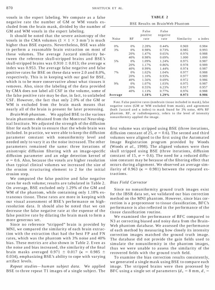
It should be noted that the severe anisotropy of thevoxels in the CMA volumes (1 3 1 3 3 mm3) is muchhigher than BSE expects. Nevertheless, BSE was ableto perform a reasonable brain extraction on most ofthese volumes. The average Jaccard similarity be-tween the reference skull-stripped brains and BSE’sskull-stripped brains was 0.910 6 0.013; the average kindex was 0.953. The average false negative and falsepositive rates for BSE on these data were 2.0 and 8.0%,respectively. This is in keeping with our goal for BSE,which is to be more conservative about what tissues itremoves. Also, since the labeling of the data providedby CMA does not label all CSF in the volume, some ofthe false positive rate may be due, in fact, to unlabeledCSF. However, the fact that only 2.0% of the GM orWM is excluded from the brain mask means thatnearly all of the brain is present for later processing.
BrainWeb phantom. We applied BSE to the variousbrain phantoms obtained from the Montreal Neurolog-ical Institute. We adjusted the strength of the diffusionfilter for each brain to ensure that the whole brain wasincluded. In practice, we were able to keep the diffusionparameter constant with nonuniformity level andneeded only to vary it as the noise increased. The otherparameters remained the same: three iterations ofanisotropic diffusion filtering with an image-specificdiffusion parameter and an edge detection kernel ofs 5 0.6. Also, because the voxels are higher resolutionthan typical clinical volumes we increased the size ofthe erosion structuring element to 2 for the initialerosion step.
We computed the false positive and false negativerates for each volume; results are tabulated in Table 2.On average, BSE excluded only 1.29% of the GM andWM of the phantom, while containing only 1.18% ex-traneous tissue. These rates are more in keeping withour visual assessment of BSE’s performance on high-resolution data. It should also be noted that we candecrease the false negative rate at the expense of thefalse positive rate by dilating the brain mask to form amore generous set.
Since no reference “stripped” brain is provided byMNI, we compared the similarity of each brain extrac-tion with the extraction that had the best FP and FNrates, which was the phantom with 3% noise and 40%bias. These metrics are also shown in Table 2. Even asthe noise and bias increased, the similarity of the finalbrain masks averaged 0.971 6 0.017 (k 5 0.985 60.034), emphasizing BSE’s ability to cope with varyingartifact levels.
Repeat studies—human subject data. We appliedBSE to three repeat T1 images of a single subject. The
first volume was stripped using BSE (three iterations,diffusion constant of 25, s 5 0.6). The second and thirdvolumes were aligned to the first using the AutomatedImage Registration program provided by Woods(Woods et al., 1998). The aligned volumes were thenskull stripped using BSE (three iterations, diffusionconstant of 15, s 5 0.6). The need for a reduced diffu-sion constant may be because of the filtering effect thatoccurs during alignment. We observed an average sim-ilarity of 0.963 (k 5 0.981) between the repeated ex-tractions.
Bias Field Corrector
Since no nonuniformity ground truth images existfor the IBSR data set, we validated our bias correctionmethod on the MNI phantom. However, since bias cor-rection is a preprocessor to tissue classification, BFC’sperformance is also reflected in the performance of thetissue classification routine.
We examined the performance of BFC compared toN3 at correcting biased and noisy data from the Brain-Web phantom database. We assessed the performanceof each method by measuring how closely its intensitycorrection images matched the ground truth image.The database did not provide the gain fields used tosimulate the nonuniformity in the phantom images,thus we were unable to assess the similarity of therecovered fields with the ground truth field.
To examine the bias correction results consistently,we generated a single mask using BSE to compare eachimage. The stripped brains were then processed byBFC using a single set of parameters (d 5 8 mm, d 5
Note. False positive rates (nonbrain tissue included in mask), falseegative rates (GM or WM excluded from mask), and agreementboth Jaccard and k index) to mask found for 3% noise, 40% RFhantom. RF, or radiofrequency, refers to the level of intensityonuniformity applied the image.
h s
c
871MRI TISSUE CLASSIFICATION
16 mm, dc 5 64 mm, ls 5 0.1) for all volumes. We alsoprocessed each stripped brain volume with N3 using itsdefault parameters.
Comparison of intensity-corrected images with aground truth requires that we allow for affine transla-tions of the image intensities because global scalings ortranslations of the image intensity will not affect in-tensity-based classification techniques. For this reasonwe compute an affine transformation that minimizesthe RMS difference between the ground truth imageand intensity corrected images being compared. ThisProcrustean metric allows for all possible scales andtranslations of a subject image’s intensity and is sim-ply
eRMS~X, X! 5 mina,b
Î 1
uVu Ok[V
~xk 2 ~axk 1 b!! 2, (37)
where X and X are the ground truth and intensity-orrected images, respectively, and V is the set of vox-
els in the brain or other region of interest. With the useof the affine transformation defined by a and b, theRMS difference between the original image and thetransformed image provides a fair comparison of per-formance between different bias-correction methods.These results are shown in Fig. 5 for both algorithmsand each available level of noise and bias. In the casesin which noise was applied with no bias, the normal-ized RMS difference metric shows that N3 and BFCboth left the phantom volumes relatively unchanged.N3 performed slightly better on the 3 and 5% noisephantoms, while BFC performed slightly better on the7 and 9% cases. In every case with simulated bias
FIG. 5. Normalized RMS error metrics as a percentage of WM grouncorrected phantom image, the N3-corrected image, and the BFC-
fields, the BFC-corrected image was closer to the orig-inal than the corresponding N3-corrected image. Inmost cases the RMS difference was very near to that ofthe unbiased image with the same level of noise, sig-nifying that we have removed most of the variationattributable to inhomogeneity effects.
Partial Volume Classifier
Internet Brain Segmentation Repository classifica-tion. We applied PVC after skull stripping by BSEand intensity normalization by BFC to the 20 normalbrain volumes from the IBSR. We performed skullstripping using one of three parameter settings. Biascorrection was performed using the same settings forall 20 brains. The selection of the tissue prior weight-ing for tissue classification was performed manually,using one of three settings. Settings were varied onlywhen the results were clearly unacceptable. No man-ual editing of the brain volume or labels was per-formed. It is possible that more tuning of the parame-ters to the individual data would have improved theresults.
To analyze the performance of our method we usedthe Jaccard similarity metric. CMA provides referencesimilarity results for several methods described by Ra-japakse and Kruggel (1998) that have been tested us-ing the IBSR data sets. The results of each method areaveraged over the 20 volumes. Since the IBSR data areclassified only into pure tissue types, we converted ourtissue classification result into a three-class (CSF, GM,and WM) labeling. We reassigned each mixed voxel bysetting its label to the pure tissue having the greatestfraction. We then computed the Jaccard similarity for
d truth intensity calculated between the ground truth image and theected image.
uncorr
f
toldnlobfW0r
ottBt
c
872 SHATTUCK ET AL.
our GM and WM sets compared to the expert labelings.The average scores over all 20 volumes for GM and WMfor the reference methods, our method, and the GMmeasure provided in Zeng et al. (1999) are shown inFig. 6 (WM metrics are not provided in Zeng et al.,1999). Also shown are reference metrics for interopera-tor variability, 0.876 for GM and 0.832 for WM, pro-posed by CMA based on an interoperator variabilitycomparison of two experts segmenting four brains. Thebrains used in that comparison were not from this dataset and do not necessarily represent the similarity thatwould be achieved by experts segmenting the 20 vol-umes we examined. The best average performance ofthe six reference methods is 0.564 for GM and 0.571 forWM. Our method produced average similarity mea-sures of 0.595 6 0.130 for GM and 0.664 6 0.107 forWM. These values equate to k indices of 0.746 6 0.114for GM and 0.798 6 0.089 for WM. The GM similaritymeasure for the coupled surface result on the wholebrain is 0.657, which outperforms our method (Zeng etal., 1999). While none of the methods reach the targetperformance suggested by CMA, all of these methodsshould achieve better performance on more recentlyacquired data, with voxel dimensions that are lessanisotropic. Our results on the BrainWeb phantomsupport this.
BrainWeb phantom classification. We used theBFC software on each of the available BrainWeb phan-toms after skull stripping with BSE. We then com-puted labelings and fractional tissue values for eachimage using the PVC software. We generated three-
FIG. 6. Comparison of BSE/BFC/PVC to other methods on the IBoupled surfaces method).
class labelings for both the ground truth labeling andour labeled results by reassigning each voxel with thepure tissue label having the largest fraction for thatvoxel. We then computed the Jaccard similarity coeffi-cient for the GM and WM sets for each volume com-pared to the ground truth; these results are shown inFig. 7. The average Jaccard scores for these 12 volumeswere 0.808 6 0.063 for GM and 0.867 6 0.063 for WM.These numbers are approaching interoperator vari-ability levels suggested by CMA. The average k indiceswere k 5 0.893 6 0.041 for GM and k 5 0.928 6 0.039or WM.
Our method performed well on most volumes fromhis data set, and Fig. 7 demonstrates the robustness ofur method on these data in the presence of varyingevels of the applied nonuniformity. Our method pro-uced relatively poor results for one volume, the 9%oise, 0% RF phantom. In this case, examination of the
abeled volume revealed that the MAP classifier hadversmoothed the labeling. By reducing the prior to5 0.01, we were able to improve the Jaccard metric
or this classification to 0.735 for GM and 0.818 forM, which improved the average scores slightly to
.816 6 0.044 and 0.878 6 0.033 for GM and WM,espectively.Partial volume fraction results. To assess our meth-
d’s performance at computing partial volume frac-ions, we compared our fractional images to the groundruth fractional volumes provided by MNI for theirrainWeb phantom. We computed the RMS error be-
ween two fractional volumes X and Y as
data set (WM values are not provided by Zeng et al., 1999, for the
SR
873MRI TISSUE CLASSIFICATION
efrac~X, Y! 5 Î 1
uVu Ok[V
uyk 2 xku 2, (38)
where V is the region of the brain mask. These resultsare provided in Table 3 for the MAP and ML classifiedresults. In every case, we saw an improvement in thismetric comparing the MAP results to the ML results.
Pham and Prince (1999) studied the performanceof several tissue classification methods using theBrainWeb phantom. They applied each technique tophantoms with 3% noise and 0, 20, and 40% RFnonuniformity fields, then computed the mean-squared error (MSE) for the GM fractional result ofeach method on each simulated image. The best re-
FIG. 7. Similarity metrics for BSE/BFC/PVC processed ph
Note. RMS error of the fractional voxel content computed by BSE
sult on the 0% RF volume was 0.0194 as classified bythe fuzzy C-means (FCM) method. The truncated-multigrid FCM algorithm had the best performanceon the 20 and 40% RF volumes, with MSE metrics of0.0214 and 0.0244, respectively. Our method pro-duced MSE results for these three images of 0.0188,0.0192, and 0.0252. It should be noted that a directcomparison cannot be made since we use a differentbrain mask, and therefore a different region for theMSE computation, from what was used by Pham andPrince. Nevertheless, these metrics do suggest thatour algorithm would be competitive with the best ofthese methods. Figure 8 shows images of the frac-tional volume computed for a real MR volume.
om volumes compared to the ground truth tissue labelings.
Using the similarity measures on real and phantomdata, we have shown the methods described in thispaper to be accurate. Additionally, our methods havebeen implemented in a computationally efficient man-ner. On an Intel 933-MHz Pentium III Xeon processorwith 256 MB of RAM, the entire process of skull strip-ping, bias correcting, and classifying a brain typicallytakes less than 5 min. For the IBSR collection of data,the average computation times for each brain were5.1 s for BSE, 51.8 s for BFC, and 3.4 s for PVC. TheBrainWeb phantom represents a much more typicalvolume with image dimensions of 181 3 217 3 181. Onaverage, BSE took 10 s for skull stripping, BFC took 2min 20 s, and PVC took 25 s, for a total processing timeof less than 3 min per volume on these data.
CONCLUSION
We have presented a three-stage sequence of tech-niques for identifying and classifying the brain tissueswithin a T1-weighted MRI of the human head. Themethod makes use of low-level methods and providesinformation at the voxel level regarding the tissue con-tent of the image. We validated our method on phan-tom and real human data and demonstrated that itoutperformed several published methods.
ACKNOWLEDGMENT
This work was supported in part by the National Institute ofMental Health Grants RO1-MH53213 and P50-MH57180.
REFERENCES
Baillet, S., Mosher, J., Leahy, R., and Shattuck, D. 1999. Brainstorm:A Matlab toolbox for the processing of MEG and EEG signals.NeuroImage 9:S246.
Bajcsy, R., and Kovacic, S. 1989. Multi-resolution elastic matching.Comput. Vision Graph. Image Processing 46:1–21.
Bajcsy, R., Lieberson, R., and Reivich, M. 1983. A computerizedsystem for elastic matching of deformed radiographic images toidealized atlas images. J. Comput. Assisted Tomogr. 7:618–625.
Bartels, R., Beatty, J., and Barsky, B. 1987. An Introduction toSplines for Use in Computer Graphics and Geometric Modeling.Kaufmann, Los Altos, CA.
Bertsekas, D. 1995. Nonlinear Programming. Athena Scientific, Bos-ton.
Besag, J. 1986. On the statistical analysis of dirty pictures. J. R.Stat. Soc. B 48:259–302.
Bomans, M., Hohne, K., Tiene, U., and Riemer, M. 1990. 3-D seg-mentation of MR images of the head for 3-D display. IEEE Trans.Med. Imag. 9:177–183.
Bonar, D. C., Schaper, K. A., Anderson, J. R., Rottenberg, D. A., andStrother, S. C. 1993. Graphical analysis of MR feature space formeasurement of CSF, gray-matter, and white-matter volumes.J. Comput. Assisted Tomogr. 17:461–470.
Brinkmann, B. H., Manduca, A., and Robb, R. A. 1998. Optimizedhomomorphic unsharp masking for MR grayscale inhomogeneitycorrection. IEEE Trans. Med. Imag. 17:161–171.
Brummer, M. E., Merseau, R. M., Eisner, R. L., and Lewine, R. R. J.1993. Automatic detection of brain contours in MRI data sets.IEEE Trans. Med. Imag. 12:153–166.
Choi, H. S., Haynor, D. R., and Kim, Y. 1991. Partial volume tissueclassification of multi-channel magnetic resonance images—Amixel model. IEEE Trans. Med. Imag. 10:395–407.
Christensen, G. E. 1999. Consistent linear-elastic transformationsfor image matching. In Lecture Notes in Computer Science, Vol.1613, Proceedings of the 16th International Conference on Infor-mation Processing in Medical Imaging (A. Kuba, M. Samal, and A.Todd-Pokropek, Eds.), pp. 224–237. Springer-Verlag, Berlin/Hei-delberg.
Christensen, G. E., Rabbitt, R. D., and Miller, M. I. 1996. Deformabletemplates using large deformation kinematics. IEEE Trans. ImageProcessing 5:402–417.
Collins, D., Zijdenbos, A., Kollokian, V., Sled, J., Kabani, N., Holmes,C., and Evans, A. 1998. Design and construction of a realisticdigital brain phantom. IEEE Trans. Med. Imag. 17:463–468.
Collins, D. L., Zijdenbos, A. P., Baare, W. F., and Evans, A. C. 1999.ANIMAL1INSECT: Improved cortical structure segmentation. InLecture Notes in Computer Science, Vol. 1613, Proceedings of the16th International Conference on Information Processing in Med-ical Imaging (A. Kuba, M. Samal, and A. Todd-Pokropek, Eds.), pp.210–223. Springer-Verlag, Berlin/Heidelberg.
Dale, A. M., Fischl, B., and Sereno, M. I. 1999. Cortical surface-basedanalysis. I. Segmentation and surface reconstruction. NeuroImage9:179–194.
Dale, A. M., and Sereno, M. I. 1993. Improved localization of corticalactivity by combining EEG and MEG with MRI cortical surfacereconstruction: A linear approach. J. Cognit. Neurosci. 5:162–176.
Davatzikos, C. 1997. Spatial transformation and registration ofbrain images using elastically deformable models. Comput. VisionImage Understand. 66:207–222.
Dawant, B. M., Zijdenbos, A. P., and Margolin, R. A. 1993. Correctionof intensity variations in MR images for computer-aided tissueclassification. IEEE Trans. Med. Imag. 12:770–781.
DeCarli, C., Murphy, D. G. M., Teichberg, D., Campbell, G., andSobering, G. S. 1996. Local histogram correction of MRI spatiallydependent image pixel intensity nonuniformity. J. Magn. Reson.Imag. 6:519–528.
Deriche, R. 1987. Using Canny’s criteria to derive a recursivelyimplemented optimal edge detector. Int. J. Comput. Vision 1:167–187.
Dice, L. 1945. Measures of the amount of ecologic association be-tween species. Ecology 26:297–302.
Duda, R. O., and Hart, P. E. 1973. Pattern Classification and SceneAnalysis. Wiley, New York.
Gerig, G., Kubler, O., Kikinis, R., and Jolesz, F. 1992. Nonlinearanisotropic filtering of MRI data. IEEE Trans. Med. Imag. 11:221–232.
Guillemaud, R., and Brady, M. 1997. Estimating the bias field of MRimages. IEEE Trans. Med. Imag. 16:238–251.
Guttmann, C., Jolesz, F. A., Kikinis, R., Killiany, R., Moss, M.,Sandor, T., and Albert, M. 1998. White matter changes with nor-mal aging. Neurology 50:972–978.
Heindel, W. C., Jernigan, T. L., Archibald, S. L., Achim, C. L.,Masliah, E., and Wiley, C. A. 1994. The relationship of quantita-tive brain magnetic resonance imaging measures to neuropatho-logic indexes of human immunodeficiency virus infection. Arch.Neurol. 51:1129–1135.
876 SHATTUCK ET AL.
Ibanez, V., Pietrini, P., Alexander, G. E., Furey, M., Teichberg, D.,Rajapakse, J., Rapoport, S., Schapiro, M., and Horowitz, B. 1998.Regional glucose metabolic abnormalities are not the result ofatrophy in Alzheimer’s disease. Neurology 50:1585–1593.
John, F. 1982. Partial Differential Equations, 4th ed. Springer-Ver-lag, New York.
Kapur, T., Grimson, W. E. L., Wells, W. M., and Kikinis, R. 1996.Segmentation of brain tissue from magnetic resonance images.Med. Image Anal. 1:109–127.
Koepp, M. J., Richardson, M. P., Labbe, C., Brooks, D. J., Cunning-ham, V. J., Ashburner, J., Paesschen, W. V., Resevz, T., andDuncan, J. S. 1997. 11C-Flumazenil PET, volumetric MRI, andquantitative pathology in mesial temporal lobe epilepsy. Neurol-ogy 49:764–773.
Kruggel, F., and von Cramon, D. 1999. Alignment of magnetic-resonance brain datasets with the stereotactical coordinate sys-tem. Med. Image Anal. 3:175–185.
Laidlaw, D. H., Fleischer, K. W., and Barr, A. H. 1998. Partial-volume Bayesian classification of material mixtures in MR volumedata using voxel histograms. IEEE Trans. Med. Imag. 17:74–86.
Leahy, R., Hebert, T., and Lee, R. 1991. Applications of Markovrandom fields in medical imaging. In Proceedings of the 11th In-ternational Conference on Information Processing in Medical Im-aging (D. A. Ortendahl and J. Llacer, Eds.), pp. 1–14. Wiley–Liss,New York.
Mackiewich, B. 1995. Intracranial Boundary Detection and RadioFrequency Correction in Magnetic Resonance Images. SimonFraser Univ., Burnaby, British Columbia, Canada. [Ph.D. thesis]
Marr, D., and Hildreth, E. 1980. Theory of edge detection. Proc. R.Soc. London 207(B):187–217.
Miller, M., Amit, Y., Christensen, G. E., and Grenander, U. 1993.Mathematical textbook of deformable neuroanatomies. Proc. Nat.Acad. Sci. USA 90:11944–11948.
Nocera, L., and Gee, J. C. 1997. Robust partial-volume tissue clas-sification of cerebral MRI scans. In SPIE Medical Imaging 1997(K. M. Hanson, Ed.), Vol. 3034, pp. 312–322. SPIE, Bellingham,WA.
Ozkan, M., Dawant, B. M., and Maciunas, R. J. 1993. Neural-network-based segmentation of multi-model medical images: A comparativeand prospective study. IEEE Trans. Med. Imag. 12:534–544.
Perona, P., and Malik, J. 1990. Scale-space and edge detection usinganisotropic diffusion. IEEE Trans. Pattern Anal. Mach. Intell.12:629–639.
Pham, D., and Prince, J. 1999. Adaptive fuzzy segmentation of mag-netic resonance images. IEEE Trans. Med. Imag. 18:737–752.
Rajapakse, J. C., and Kruggel, F. 1998. Segmentation of MR imageswith intensity inhomogeneities. Image Vision Comput. 16:165–180.
Rusinek, H., de Leon, M. J., George, A. E., Stylopoulos, L. A., Chan-dra, R., Smith, G., Rand, T., Mourino, M., and Kowalski, H. 1991.Alzheimer disease: Measuring loss of cerebral gray matter withMR imaging. Radiology 178:109–114.
Sandor, S., and Leahy, R. 1997. Surface-based labeling of corticalanatomy using a deformable database. IEEE Trans. Med. Imag.16:41–54.
Sandor, S. R. 1994. Atlas of Guided Deformable Models for AutomaticAnatomic Labeling of Magnetic Resonance Brain Images. Univ. ofSouthern California, Los Angeles. [Ph.D. thesis]
Santago, P., and Gage, H. D. 1993. Quantification of MR brainimages by mixture density and partial volume modeling. IEEETrans. Med. Imag. 12:566–574.
Shattuck, D. W. 2000. Automated Segmentation and Analysis ofHuman Cerebral Cortex Imagery. Univ. of Southern California,Los Angeles. [Ph.D. thesis]
Sled, J. G., and Pike, G. B. 1998. Understanding intensity non-uniformity in MRI. In Medical Image Computing and Computer-Assisted Intervention-MICCAI ’98, Lecture Notes in Computer Sci-ence (W. M. Wells, A. C. F. Colchester, and S. Delp, Eds.), pp.614–622. Springer-Verlag, Berlin/Heidelberg.
Sled, J. G., Zijdenbos, A. P., and Evans, A. C. 1998. A nonparametricmethod for automatic correction of intensity nonuniformity in MRIdata. IEEE Trans. Med. Imag. 17:87–97.
Thaler, H., Ferber, P., and Rottenberg, D. A. 1978. A statisticalmethod for determining proportions of gray matter, white matter,and CSF using computed tomography. Neuroradiology 16:133–135.
Thompson, P. M., MacDonald, D., Mega, M. S., Holmes, C. J., Evans,A. C., and Toga, A. W. 1998. Detection and mapping of abnormalbrain structure with a probabilistic atlas of cortical surfaces.J. Comput. Assisted Tomogr. 21:567–581.
Van Leemput, K., Maes, F., Vandermeulen, D., and Suetens, P.1999a. Automated model-based bias field correction of MR imagesof the brain. IEEE Trans. Med. Imag. 18:885–896.
Van Leemput, K., Maes, F., Vandermeulen, D., and Suetens, P.1999b. Automated model-based tissue classification of MR imagesof the brain. IEEE Trans. Med. Imag. 18:897–908.
Warfield, S. K., Westin, C.-F., Guttmann, C. R. G., Albert, M., Jolesz,F. A., and Kikinis, R. 1999. Fractional segmentation of whitematter. In Medical Image Computing and Computer-Assisted In-tervention-MICCAI ’99, Lecture Notes in Computer Science (C.Taylor and A. Colchester, Eds.), pp. 928–935. Springer-Verlag,Berlin/Heidelberg.
Wells, W. M., Grimson, W. E. L., Kikinis, R., and Jolesz, F. A. 1996.Adaptive segmentation of MRI data. IEEE Trans. Med. Imag.15:429–442.
Woods, R. P., Grafton, S. T., Holmes, C. J., Cherry, S. R., andMazziotta, J. C. 1998. Automated image registration. I. Generalmethods and intrasubject, intramodality validation. J. Comput.Assisted Tomogr. 22:141–154.
Wu, Z., and Leahy, R. 1991. A graph theoretic approach to tissueclassification in MR images. In Proceedings of the SPIE, Vol. 1450,Biomedical Image Processing II. (A. C. Bovik and V. Howard,Eds.), pp. 120–132. SPIE, Bellingham, WA.
Yan, M. X. H., and Karp, J. S. 1995. An adaptive Bayesian approachto three-dimensional MR brain segmentation. In Information Pro-cessing in Medical Imaging (Y. Bizais, C. Barillot, and R. D. Paola,Eds.), pp. 201–213. Kluwer Academic, Dodrecht.
Zeng, X., Staib, L. H., Schultz, R. T., and Duncan, J. S. 1999. Seg-mentation and measurement of the cortex from 3D MR imagesusing coupled surfaces propagation. IEEE Trans. Med. Imag. 18:100–111.
Zijdenbos, A. P., Dawant, B. M., Margolin, R. A., and Palmer, A. C.1994. Morphometric analysis of white matter lesions in MR im-ages. IEEE Trans. Med. Imag. 13:716–724.