Magneto-optical trap of 39K: setup andcharacterisationReport of a 36 EC master project

Tom Opdam (5696011)

Supervisors: Prof. dr. J.T.M. WalravenDr. V. LebedevDr. S. Lepoutre

project realised during 1-10-2011 until 19-04-2012

Universiteit van AmsterdamFaculteit der Natuurwetenschappen, Wiskunde en Informatica

van der Waals-Zeeman Instituut

Abstract

During this six months project a three-dimensional magneto-optical trap (MOT)for the bosonic isotope 39K has been realised. The three-dimensional MOT is loadedby a pre-cooled atomic beam originating from a two-dimensional MOT. A frequency-modulation spectroscopy setup was built to obtain a feedback signal that stabilizesthe frequency of the laser. A characterization of the MOT is made by analysing thefluorescence images of the atom cloud produced with a CCD camera. Among theinvestigated parameters are the lifetime, loading time and the total number of trappedatoms in the 3D MOT. Based on the results, possible modifications of the setup areproposed for an improvement of the performance of the MOT.

1

Contents

1 Introduction 41.1 Outline . . . . . . . . . . . . . . . . . . . . . . . . . . . . . . . . . . . . . . 5

2 Theoretical background 52.1 Chapter overview . . . . . . . . . . . . . . . . . . . . . . . . . . . . . . . . . 52.2 Potassium and its energy levels scheme . . . . . . . . . . . . . . . . . . . . . 5

2.2.1 Potassium . . . . . . . . . . . . . . . . . . . . . . . . . . . . . . . . . 52.2.2 Fine and Hyperfine structure . . . . . . . . . . . . . . . . . . . . . . 62.2.3 Natural linewidth . . . . . . . . . . . . . . . . . . . . . . . . . . . . . 9

2.3 Spectroscopy . . . . . . . . . . . . . . . . . . . . . . . . . . . . . . . . . . . 102.3.1 Doppler shift and Doppler width . . . . . . . . . . . . . . . . . . . . 102.3.2 Doppler-free saturated absorption spectroscopy . . . . . . . . . . . . 122.3.3 Frequency modulation spectroscopy . . . . . . . . . . . . . . . . . . 14

2.4 Gaussian optics . . . . . . . . . . . . . . . . . . . . . . . . . . . . . . . . . . 172.4.1 Gaussian beam . . . . . . . . . . . . . . . . . . . . . . . . . . . . . . 172.4.2 Higher order transverse modes . . . . . . . . . . . . . . . . . . . . . 182.4.3 The Fabry-Perot cavity . . . . . . . . . . . . . . . . . . . . . . . . . 192.4.4 The confocal cavity . . . . . . . . . . . . . . . . . . . . . . . . . . . 202.4.5 Mode degeneracy in the confocal cavity . . . . . . . . . . . . . . . . 21

2.5 Laser cooling and trapping . . . . . . . . . . . . . . . . . . . . . . . . . . . 232.5.1 Overview . . . . . . . . . . . . . . . . . . . . . . . . . . . . . . . . . 232.5.2 Scattering force . . . . . . . . . . . . . . . . . . . . . . . . . . . . . . 232.5.3 Magneto-Optical Trap . . . . . . . . . . . . . . . . . . . . . . . . . . 252.5.4 MOT’s for multilevel atoms . . . . . . . . . . . . . . . . . . . . . . . 27

2.6 MOT dynamics . . . . . . . . . . . . . . . . . . . . . . . . . . . . . . . . . . 28

3 Experimental setup 303.1 Chapter overview . . . . . . . . . . . . . . . . . . . . . . . . . . . . . . . . . 303.2 Vacuum system . . . . . . . . . . . . . . . . . . . . . . . . . . . . . . . . . . 303.3 Master Laser . . . . . . . . . . . . . . . . . . . . . . . . . . . . . . . . . . . 313.4 Experimental setup spectroscopy . . . . . . . . . . . . . . . . . . . . . . . . 323.5 Laser locking setup . . . . . . . . . . . . . . . . . . . . . . . . . . . . . . . . 343.6 Laser system . . . . . . . . . . . . . . . . . . . . . . . . . . . . . . . . . . . 353.7 39K 2D MOT . . . . . . . . . . . . . . . . . . . . . . . . . . . . . . . . . . . 373.8 39K 3D MOT . . . . . . . . . . . . . . . . . . . . . . . . . . . . . . . . . . . 393.9 Fluorescence imaging . . . . . . . . . . . . . . . . . . . . . . . . . . . . . . . 40

2

4 Results 414.1 Chapter overview . . . . . . . . . . . . . . . . . . . . . . . . . . . . . . . . . 414.2 Spectroscopy results . . . . . . . . . . . . . . . . . . . . . . . . . . . . . . . 414.3 Laser-locking performance . . . . . . . . . . . . . . . . . . . . . . . . . . . . 444.4 Fluorescence measurement with a CCD camera . . . . . . . . . . . . . . . . 454.5 MOT parameters as a function of the magnetic field gradient . . . . . . . . 494.6 MOT lifetime . . . . . . . . . . . . . . . . . . . . . . . . . . . . . . . . . . . 524.7 MOT loading time . . . . . . . . . . . . . . . . . . . . . . . . . . . . . . . . 54

5 Conclusions and Outlook 56

6 Update 22-04-2013 57

Bibliography 58

3

1 Introduction

A remarkable aspect of quantum mechanics is that it tells us that all matter around usfalls in either one of two categories, bosons or fermions. There are important differencesbetween these two fundamental particles. Bosons, with integer spin, are described by Bose-Einstein statistics. Fermions, with half-integer spin, obey Fermi-Dirac statistics. In 1925,Einstein predicted that bosons for temperatures near absolute zero, in the order of nanoKelvin, condens into the ground state of the system, forming a Bose-Einstein condensate(BEC) [1]. This is in contrast with their counter-particles, the fermions, for which theFermi-Dirac statistics state that indentical fermions can not occupy the same quantumstate at any time. Therefore, for temperatures near absolute zero, fermions do not forma condensate of particles in the same ground state, but they each occupy one state up tothe Fermi energy, forming a Fermi degenerate gas. These quantum mechanical phenomenathat occur near absolute zero temperature present an opportunity to investigate quantummechanical effects with macroscopic entities. The experimental realisation of bosonic andfermionic ensembles at temperatures in the order of nano Kelvins has proved to be a chal-lenging one. In 1995, seventy years after Einsteins prediction, experimentalists were ableto cool bosons for the first time to degeneracy, realizing the first Bose-Einstein condensatein a dilute atomic gas [2], [3]. It took another four years to demonstrate the first fermionicdegenerate gas, [4].

In those seventy years from prediction to realisation, probably the most importantinvention that contributed to the creation of degenerate gases, was the laser. Since theinteraction of atoms with light forms the most important mechanism for the creation andmanipulation of ultracold atoms, the laser, capable of emitting narrow band light, is atthe basis of many experimental schemes in which atoms are trapped and cooled. A crucialstep towards quantum degeneracy was made in 1986, when trapping of neutral atoms witha device called the magneto-optical trap (MOT) was made possible [5]. MOT’s make useof optical forces that are exerted on atoms that experience Zeeman shifts in the presenceof a position dependent magnetic field. The frequency of the laser light that is used isrequired to be stabilized with respect to a specified atomic transition, with an accuracybelow the natural linewith of the transition. A MOT provides experimentalists with atomsat temperatures in the order of micro Kelvins. Not yet cold enough for degeneracy tooccur, but a great starting point for ultracold gas experiments.

In this project, the cooling and trapping of a bosonic potassium isotope, 39K, is demon-strated. MOT’s for potassium-39 have already been built in numerous groups, with variousloading techniques. In our setup we have chosen a two-dimensional MOT as a cold atomsource to provide an atomic beam that loads the MOT in a ultra high vacuum chamber.

4

1.1 Outline

In chapter 2, the theoretical background required for the description of the work done inthis project is discussed. Among the covered subjects are the properties of potassium-39,saturation absorption spectroscopy, frequency-modulation spectroscopy, Gaussian beams,the Fabry-Perot interferometer and the principles of laser cooling and trapping. In chapter3, a detailed description is given of the experimental setup used in this project. The resultsof the measurements, their interpretation and comparisons with other work are presentedin chapter 4. Finally, conclusions are drawn and an outlook on future experimental stepsis given in chapter 5.

2 Theoretical background

2.1 Chapter overview

In this chapter a brief review of the theory used in this project is given. The chapter isdivided into four parts. As a starting point, in section 2.2, an introduction to the potassiumatom is made and several concepts of atomic physics are given. In section 2.3, the topic ofspectroscopy and its applications to laser locking are addressed. Gaussian beams and theirrelation with the Fabry-Perot interferometer are discussed in section 2.4. In the last sectionof this chapter, section 2.5, the principles of cooling and trapping of atoms are covered,leading to a discussion of the main object in this project, the magneto optical trap.

2.2 Potassium and its energy levels scheme

2.2.1 Potassium

Potassium is an alkali metal denoted with the symbol K (after the Latin name Kalium)and has an atomic number of 19. Like all other alkali metals, it has one electon in theoutermost shell, giving the atom a low ionization energy. Because of this low ionizationenergy, potassium is chemically reactive. It oxidizes rapidly with air and is reactive withwater. Therefore, special care has to be taken when assembling glass ampules containingpotassium. An overview of the different naturally occurring potassium isotopes is presentedin table 1. Whereas 39K and 41K are bosonic isotopes, 40K is a fermionic isotope. Togetherwith 6Li it is the only stable fermionic alkali isotope, making it a popular atom for ultracoldfermionic experiments [6]. However, in this project the atom of interest is the bosonicisotope 39K, since its high natural abundance is practically favourable for trapping a highnumber of cold atoms.

5

Isotope A Neutrons N Abundance (%) m(u) I

39 20 93.2581 38.9637 3/2 bosonic

40 21 0.0117 39.9639 4 fermionic

41 22 6.7302 40.96182 3/2 bosonic

Table 1: Several properties of the naturally occurring potassium isotopes. The atomicnumber Z of potassium is 19. The given properties are: the mass number A, the numberof neutrons N , the abundance in %, the atomic mass m and the nuclear spin I. Valuestaken from [7].

2.2.2 Fine and Hyperfine structure

The fine structure of an alkali atom is the result of the coupling between the orbital angularmomentum L of the valence electron and its spin angular momentum S. The total angularmomentum of the electron is given by

J = L + S, (1)

with the condition that the quantum number J of J lies in the range

|L− S| ≤ J ≤ L+ S. (2)

The Hamiltonian describing the fine structure for hydrogen-like atoms is given by

HLS = ξ(r)L · S, (3)

here ξ(r) is the coupling constant. The eigenvalues of this Hamiltonian can be calculatedwith the operator identity

L · S =1

2(J2 + L2 + S2). (4)

It follows that the eigenvalues of the fine structure Hamiltonian for hydrogen-like atomsare proportional to

∆Efs(n2s+1LJ) ∝ 1

2[j(j + 1)− l(l + 1)− s(s+ 1)]. (5)

Here, j, l and s are the quantum numbers associated with J, L and S. (For alkali atomsonly the valence electron contributes to the angular momentum of the atom and the con-vention is that the angular momentum of one electron is indicated in lower case [8].) Itfollows from equation (5) that fine splitting only occurs if l 6= 0.

In the case of 39K, the electronic groundstate is 42S1/2, with L = 0 and S = 1/2 and

6

therefore J = 1/2. For the first excited state L = 1 and S = 1/2, thus J = 1/2 or J = 3/2,corresponding to the states 2P1/2 and 2P3/2. The fine structure lifts the degeneracy ofthese first excited states. The transition 42S1/2 → 2P1/2 is called the D1 transition andthe transition 42S1/2 → 2P3/2 is called the D2 transition.

Besides the spin-orbit coupling, one should als take into account the coupling betweenthe nuclear spin I and the total electronic angular momentum. The total angular momen-tum is given by

F = J + I. (6)

where the quantum number F , associated with the operator F, must lie in the range:

|J − I| ≤ F ≤ J + I. (7)

The Hamiltonian for the hyperfine structure is given by

Hhfs =ahfs~2

I · J +bhfs~2

3(I · J)2 + 32I · J + I2J2

2I(2I − 1)J(2J − 1). (8)

where ahfs is the magnetic-dipole constant and bhfs is the electric-quadrupole couplingconstant.In a similar way as for the fine structure, the dot product I · J can be written as 1

2(J2 +L2 + S2) and this leads to an hyperfine energy shift of

∆Ehfs(n2s+1LJ) =

ahfs2K + bhfs

32K(K + 1)− 2I(I + 1)J(J + 1)

2I(2I − 1)J(2J − 1). (9)

where K = F (F + 1)− I(I + 1)− J(J + 1).In contrast to the fine structure, the energy levels in the hyperfine structure split also

when L = 0. This is the reason that the ground state of 39K with J = 1/2 and I = 3/2is split in two levels, the states 4S1/2(F = 1) and 4S1/2(F = 2). In figure 1, the fineand hyperfine structure of the three natural abundant potassium isotopes are shown. Thestrongest spectral lines of the ground state potassium atoms are the D1 line (2S1/2 → 2P1/2)and the D2 line (2S1/2 → 2P3/2). The values of the optical transition frequencies in figure1 are taken from Falke et al., who have published their high precision measurements of thepotassium energy levels in [9]. It should be noted that the hyperfine structure of the 40Kisotope is inverted. This a result of its negative magnetic-dipole coupling constant. Both39K and 41K have a positive magnetic-dipole coupling constant and thus a non-invertedhyperfine structure.

7

Figure 1: The fine- and hyperfine structure of 39K, 40K and 41K. The hyperfine structure ofof 40K is inverted due to its negative magnetic dipole constant, ahfs. Both other isotopeshave a postive magnetic dipole constant and thus a non-inverted hyperfine structure. Figuretaken from [7].

8

Each of the hyperfine energy levels consists of 2F + 1 magnetic sublevels. Without anexternal magnetic field these sublevels are degenerate. However, when an external magneticfield is aplied, the degeneracy is lifted due to the Zeeman effect. The Zeeman Hamiltonianis given by

HZ =µB~

(gJJ− gII) ·B, (10)

where µB is the Bohr-magneton, gJ is the Lande factor for an electron and gI is thenuclear gyromagnetic factor. The total hyperfine interaction in the presence of an externalmagnetic field is thus given by the Hamiltonian

H = Hhfs +HZ . (11)

For weak magnetic fields the I-J coupling is still present and the total angular momentumF precesses around the direction of the magnetic field. In that case the Hamiltonian HZ

perturbs the zero-field eigenstates of Hhfs and the energy levels split linearly according to

∆EB,lowZ = µBgFmFB , (12)

where gF is given by

gF = gJF (F + 1) + J(J + 1)− I(I + 1)

2F (F + 1)+ gI

F (F + 1) + I(I + 1)− J(J + 1)

2F (F + 1). (13)

In the case of a high magnetic field the I-J coupling is lifted. Both angular momentaprecess independently around the direction of the magnetic field. The energy shift in thisregime is called the Paschen-Back effect and is approximated by [10]

∆EB,highZ = µBgJmJ + ahfsmImJ + bhfs3(mJmI)

2 + 32mJmI − I(I + 1)J(J + 1)

2J(2J − 1)I(2I − 1). (14)

The magnetic crossover field where the energy of the states in the low-field approximationequals the energy in the high-field approximation is much higher than the magnetic fieldused in a magneto optical trap. Therefore, the linear low-field approximation is valid todescribe the energy shifts of cold atoms in the MOT.

2.2.3 Natural linewidth

The difference between two atomic energy levels can be overcome by the absorption oremission of a photon with the same energy, E = ~ω0, where ω0 is the transition frequency.

9

However, because of the generally short lifetimes of excited states, the uncertainty relation∆E∆t > ~

2 tells us that there is a significant uncertainty in the measured energy, andthus in the measured transition frequency. Emission and absorption lines have thereforefinite widths that are called natural linewidths. These are the full widths at half maximum(FWHM) of the absorption/emission peaks, usually denoted by the symbol Γ. Naturallinewidths have a Lorentzian profile.

In the case of 39K, the D2-line has a lifetime of τ ≈ 26.37× 10−9 s. This correspondsto a natural linewidth Γ/2π ≈ 6.03 MHz [7].

2.3 Spectroscopy

In the field of laser cooling and trapping, spectroscopy plays an important role. For mostexperiments it is of great importance that the main parameters; i.e., frequency and inten-sity, of the laser are stabilized. Moreover, many experiments require control of the laserfrequency to a fraction of the linewidth of atomic transitions, which typically has a widthin the order of MHz. Fluctuations in the laser diode current and temperature result infrequency fluctuations. Mechanical vibrations also have to be taken into account. To com-pensate for these fluctuations, lasers have to be actively stabilized. A number of differentspectroscopy techniques exist in order to accomplish this. In this project we chose to usefrequency modulation (FM) spectroscopy (see section 2.3.3) to deduce a so-called errorsignal that is needed for laser stabilization.

Typical spectroscopy works as follows. Laser light is sent through an ensemble ofatoms. If the photon energy, E = ~ω, matches the energy difference between two atomstates, the photons are absorbed or emitted. This absorption can be measured with theuse of a photodiode that converts light intensity into current. In this way information isgathered about the internal structure of atoms. This information can be used to providefeedback to a laser system and thereby stabilizing its main parameters.

In the following sections several aspects of spectroscopy and the principle of FM-spectroscopy will be explained.

2.3.1 Doppler shift and Doppler width

In general, the natural linewidth can not be observed without special techniques, because itis completely concealed by broadening effects that broaden the linewidth of absorption linesin atomic spectra. Doppler broadening is one of the major contributions to the spectrallinewidth of atomic gases at room temperature [11], due to the thermal motion of theatoms.

Consider an atom with transition frequency ω0. If this atom moves with a velocityv across a plane electro-magnetic wave, the absorption frequency is shifted. The wavefrequency ω in the restframe is seen in the reference frame of the moving atom as

10

ω′ = ω − k · v, (15)

where k is the wavevector of the radiation with magnitude k = ω/c = 2π/λ, and v isthe velocity of the moving atom. It is the component of the velocity along k that leadsto the Doppler effect. The atom can only absorb a photon if ω′ is equal to the transitionfrequency ω0. Hence, the frequency at which absorption could occur is

ω = ω0 + k · v. (16)

If we assume for simplicity that the direction of movement of the atoms coincides with thelight propagation (k ·v = kv), it means that atoms moving with velocity v absorb radiationwhen the frequency of radiation is

ω = ω0

(1 +

v

c

). (17)

Atoms in a gas move in all possible directions. As a result, the Doppler shift is differentfor individual particles. When a thermal equilibrium is reached all directions are equallyprobable; i.e., the velocity distribution of the particles is isotropic. The projection of theparticle velocity on any direction is given by a Maxwell velocity distribution [11]. Thenumber of atoms as a function of their velocity is then given by

ni(v) =Ni

u√πexp[−(vu

)2], (18)

where Ni is the number of all atoms in the lower state, u =√M/(π2kBT ) is the most

probable velocity, and kB is Boltzmann’s constant. The number of atoms as a function oftheir absorption frequency, that is shifted from ω0 to ω, is acquired by using the relation(16) between the velocity component and the frequency shift

ni(ω) =Nic

ω0u√πexp[−(c(ω − ω0)

ω0u

)2]. (19)

Since the absorbed light is proporsional to the number of atoms, the intensity profile ofDoppler broadened spectral line becomes

I(ω) = I0exp[−(c(ω − ω0)

ω0u

)2]. (20)

This is a Gaussian profile with a full width at half maximum (FWHM)

11

∆ωD = 2√ln2ω0u/c =

(ω0

c

)√8kT ln2/m, (21)

this expression is known as the Doppler width.A typical Doppler linewidth for 39K at room temperature is around ∆ωD ≈ 4.8 GHz.

A huge difference in comparison with the natural linewidth of the 39K D2 line, Γ/2π ≈ 6.03MHz.

2.3.2 Doppler-free saturated absorption spectroscopy

In order to resolve hyperfine transitions in spectroscopy spectra, one needs to have a spec-tral resolution that is not limited by the Doppler-width. Doppler-free saturated absorptionspectroscopy is a spectroscopy method that is capable of doing this. It will be explainedhere, because it is an important part of the spectroscopy method that we used in thisproject.

In saturated Doppler-free absorption spectroscopy, two beams are used; a weak probebeam and a stronger pump beam. The beams propagate in opposite directions and overlapin an atomic vapor cell. Both beams come from the same laser and the frequency of thelaser is scanned. After passing through the vapor cell the probe beam is sent to a photodi-ode, so that the intensity of the transmitted probe beam can be monitored. If there was nopump beam, and the laser would be scanned, an ordinary Doppler linewidth would be seen,obscuring the hyperfine transitions. The addition of a pump beam, eliminates the Dopplerlinewidth in atomic spectra and therefore resolves the hyperfine transitions. The pumpbeam passes through the vapor cell, with an intensity high enough to saturate a certainatomic transition. This means that the transmission is driven at a maximum rate which isdetermined by the lifetime of the excited state and can not be driven faster. As a result,the population density in the lower level is quickly depleted. The probe beam, with a lowerintensity, passes through the vapor cell coming from the other direction. Because of thesaturation of the absorption by the pump beam, there are few atoms left to interact withfor the probe beam. This results in a peak in the signal of the probe beam once it arrivesat the photodiode. A typical setup for saturated absorption spectroscopy is depicted infigure 2.

12

Figure 2: A schematic representation of a typical saturation absorption spectroscopy setup.A beamsplitter (BS) divides the power of the laser in a weak probe beam and a strongpump beam. The angle between the two beams is strongly exaggerated, it is usually triedto make the beams as counter-propagating as possible. Figure adapted from [12].

Depending on the frequency of the laser, three different situations can be distinguished.First of all, if the laser has a frequency far from resonance, both beams interact with atomsin different velocity classes due to the Doppler effect. If the pump beam interacts withatoms with velocity, v, the counter-propagating probe beam interacts with atoms with ve-locity, −v. The probe beam is not affected by the pump beam and a normal Doppler lineprofile is seen. The second situation arises when the laser frequency is close to resonance,both beams interact with atoms in the same velocity class, v = 0. As a result, the intensityof the probe beam transmitted through the sample has a peak at the resonance frequency.The last situation occurs when two atomic transitions have a common lower or upper leveland their frequency difference is less than the Doppler-width, |ω1−ω2| < ∆ωD. Then, extraresonances will become visible when saturation absorption spectroscopy is applied. Theseresonances are called cross-over resonances. Assume that the laser frequency, ω, is exactlytuned halfway between two transitions ω1 and ω2, (ω1 < ω2). Then, the pump beam willbe Doppler-shifted into resonance at ω1 for atoms in the velocity class, v = (ω − ω1)c/ω1,moving in the propagation direction of the pump beam. The returning probe beam willbe Doppler-shifted into resonance at ω2 for atoms in the velocity class, v = (ω2 − ω)c/ω2,the atoms that move towards the probe beam; i.e., in the propagation direction of thepump beam. If ω = (ω1 +ω2)/2, the velocity classes that are interacted with are the sameand the saturating pump beam wil saturate these atoms and few atoms are left to interactwith for the probe beam. Therefore, besides the saturation signals at ω1 and ω2 where thevelocity class v = 0 is saturated, an additional saturation signal, the cross-over signal, canbe observed at the frequency (ω1 + ω2)/2.

13

Figure 3: A schematic subtraction of the signals from the two photodiodes detecting theprobe beam and the reference beam (figure adapted from [13]).

A useful addition that can be made to a saturation absorption spectroscopy scheme,is adding a third (weak) beam, called the reference beam. This reference beam only passesthrough the vapor cell ones and does not overlap with any other beam. The referencebeam is sent to a photodiode and gives an ordinary Doppler-width. The photocurrentsfrom both photodiodes can be subtracted, resulting in a spectrum where the Doppler-width is completely eliminated and only transition peaks and cross-over peaks are seen(figure 3).

2.3.3 Frequency modulation spectroscopy

Doppler-free saturated absorption spectroscopy makes it possible to obtain a well-resolvedatomic spectrum at room temperature that would otherwise be hidden under the Doppler-width. Intensity peaks are seen at the transition frequencies and cross-over frequencies.Having a well-resolved atomic spectrum makes it possible to lock a laser; a well definedabsorption peak could be used as a locking point. However, atomic spectra can not bedirectly used for laser locking for the following reason. To lock a laser, a dispersive signalis needed. This so-called error signal should ’tell’ the feedback system how much the fre-quency deviation is and in which direction, such that the feedback system can compensatethe change. If one wants to lock a laser to a certain atomic transition (i.e. ’on top’ of atransmission peak), an intensity measurement gives no disclosure about the direction inwhich the frequency has changed, since the measured voltage decreases in both directions.Therefore, the change of the error signal has the same sign for opposing frequency shifts.To circumvent this problem one can use the derivative of the original signal. The deriva-tive signal has zero crossings at the peaks of the original signal, thus the sign of this signalis different for opposite deviations of the laser frequency. The derivative signal makes itpossible to detect the amplitude and the direction of the change of the laser frequency, itis therefore well suited to function as an error signal.

Frequency modulation (FM) spectroscopy is a technique that can be used to obtain

14

such an error signal. In FM spectroscopy the frequency of the laser is modulated with asinusoidal signal, typically with a small peak-to-peak amplitude of several mV and witha high frequency of a about 10 kHz. This can be done either by modulating the currentof the laser or by letting the light pass through an electro-optic modulator (EOM) thatis driven at the required frequency. If the laser frequency is near a transition frequency,the modulation of the frequency causes the absorption signal to modulate synchronously;i.e., the laser frequency modulation is mapped onto the transmitted intensity. This changein intensity allows the photodiode to detect a change in frequency. The conversion fromfrequency modulation to intensity modulation is sensitive to where the center frequency,around which the laser is modulated, is located on the absorption line. If it is located ona steep slope of the absorption line, a small change in frequency will result in a significantchange in transmitted intensity. But if the center frequency is located at the top of theabsorption line, a change in frequency will result in a small change in transmitted intensity.It is this principle that makes it possible to obtain the derivative of the absorption signal(see figure 4).

Figure 4: In FM-spectroscopy, frequency modulation is converted into amplitude modu-lation of the absorption signal, FM to AM. a) center frequency located at the negativeslope of the absorption profile (AM amplitude relatively large); b) center frequency locatednear the point of maximal absorption (AM amplitude relatively small); c) center frequencylocated at positive slope (same AM amplitude as in case a, but with AM/FM relationshipreversed; d) plot of AM/FM conversion ratio as a function of frequency (effectively thederivative of the absorption profile) - figure adapted from [13].

15

The mathematical derivation of the derivative of the absorption signal can be under-stood in the following way. Let a laser frequency ω be modulated with a frequency Ω withamplitude m, the transmitted intensity IT that reaches the photodiode after passing thevapor cell can be written as

IT (ω, t) = IT (ω +m sin(Ωt)). (22)

Here we assume that the amplitude of the modulation is small and that the frequency ofmodulation is smaller than the linewidth Ω < Γ.Now IT can be expanded as a Taylor series around ω

IT (ω +m sin(Ωt)) =IT (ω) +dITdω

[m sin(Ωt)]+

1

2!

d2ITdω2

[m sin(Ωt)]2 +1

3!

d3ITdω3

[m sin(Ωt)]3... (23)

With the help of basic trigonometric identities we can combine the terms

IT (ω +m sin(Ωt)) =[IT (ω) +

m2

4

d2ITdω2

+ ...]

+ sin(Ωt)[mdITdω

+m3

8

d3ITdω3

+ ...]+

cos(2Ωt)[− m2

4

d2ITdω2

+ ...]

+ .... (24)

It can be seen that the transmitted intensity contains a DC term, a term oscillating at Ω,a term oscillating at 2Ω, etc. When phase sensitive detection is applied, the coefficients ofthe different terms can be extracted. In this case phase sensitive detection is done withthe use of a lock-in amplifier. This amplifier is given the transmitted intensity signal and aperiodic reference signal. The amplifier responds only to the part of the signal that occurswith the same frequency as the periodic reference signal. So if, in this case, the referencesignal is set at a frequency of Ω or a multiple of Ω, coefficients from different terms can beextracted from the transmitted intensity signal. If m is sufficiently small, the coefficientof the sin(Ωt) term is essentialy the first derivative of the absorption signal multiplied bym. By the same token the second derivative can be extracted from the cos(2Ωt) term andhigher order derivatives extracted from higher order terms. This is why FM spectroscopyis sometimes called derivative spectroscopy.

16

2.4 Gaussian optics

2.4.1 Gaussian beam

In optics, laser beams often occur in the form of Gaussian beams. They are a solution tothe paraxial form of the Helmholtz scalar equation, an equation that provides solutionsfor the propagation of elecromagnetic waves. Gaussian beams are beams whose transverseelectric field and intensity distributions are well aproximated by Gaussian functions. Thetransverse intensity profile of a Gaussian beam is described with the Gaussian function [14]

I(r, z) = I0

(w0

w(z)

)2

exp

(−2r2

w2(z)

), (25)

where I0 = I(0, 0) is the intensity at the center of the beam at its waist, w(z) is the beamwidth (as function of the propagation direction) which is defined as the radius where theintensity drops to 1/e2 of its maximum value and w0 is the beam width where the radiusis smallest, at the waist, see figure 5.The beam radius w(z) varies along the propagation direction according to

w(z) = w0

√1 +

(z

zR

)2

, (26)

where the origin of the z-axis is defined to coincide with the beam waist and where zR isthe Rayleigh length, defined as zR = (πw0

2)/λ, with λ being the wavelength of the light.The Rayleigh length determines the length over which the beam can propagate withoutsignificantly diverging. At a distance from the waist equal to zR, the radius of the beam is

w(zR) = w0

√2 . (27)

Figure 5: Gaussian beam width w(z) as a function of z. R(z) is the radius of curvatureof the wavefront. Notice that a wavefront at the waist is similar to that of a plane wave.(Figure taken from [15])

17

Figure 6: Several different Laguerre-Gaussian transverse modes. These modes are electro-magnetic normal modes in a Fabry-Perot cavity. The TEM00 mode has a simple Gaussianbeam profile. (Picture taken from [16])

2.4.2 Higher order transverse modes

Gaussian beams are not the only solution to the paraxial form of the Helmholtz scalarequation. Several other solutions are used for modeling laser beams. For lasers withcylindrical symmetry the transverse modes are described by a combination of a Gaussianbeam profile and a Laguerre polynomial. The intensity of a beam at a point r, φ (in polarcoordinates) is given by the formula [17]

Ipl(r, φ) = I0ρl[Llpρ

]2cos2(lφ)e−ρ, (28)

where ρ = 2r2/w2 and Llp is the Laguerre polynomial of order p and index l. In figure6, several different modes are shown. These are so-called Transverse Electro Magnetic(TEM) modes, which means that the associated beams have neither electric nor magneticfield in the direction of propagation. The TEM00 mode has a simple Gaussian profile andis referred to as the lowest order mode.

18

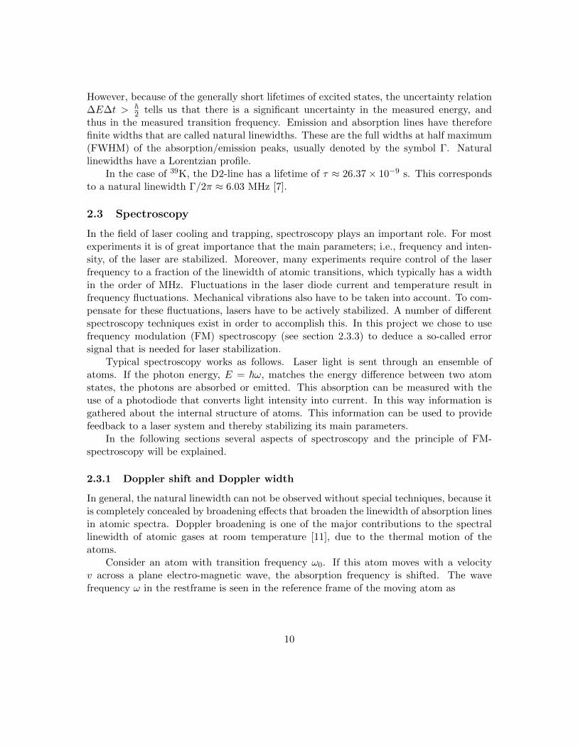
Figure 7: A plane Fabry-Perot etalon. If Θ is not 0, light ’walks-off’ in the direction parallelto the mirrors. (Figure adapted from [18])

2.4.3 The Fabry-Perot cavity

Fabry-Perot cavities (also called etalons or interferometers) are widely used instrumentsin optical physics. They are being used as sensitive wavelength discriminators, as stablefrequency references and for building up large field intensities with low input powers. Also,optical cavities are a major component of lasers, surrounding the gain medium and pro-viding feedback of the laser light. A Fabry-Perot cavity consists of two reflecting surfacesor mirrors. The ’inner’ sides of the two mirrors (the sides facing each other) are coatedfor high reflectivity. Curved mirrors are typically used because this configuration can traplight in a stable mode. Flat mirrors can also make a cavity, but it is often not a stableone, the light ’walks off’ if the incoming beam is not exactly perpendicular to the mirror,see figure 7.

The transmission function of ligth that enters a cavity depends on the interferencebetween the multiple reflections of the light between the mirrors. If the transmitted beamsare in-phase, contructive interference occurs, creating a standing wave in the cavity andresulting in a high transmission peak. If the reflected beams are out-of-phase, destructiveinterference occurs, resulting in a transmission minimum. A detailed derivation of thetransmission function in cavities is given in [19]. Whether the transmitted beams are in-phase or not depends on the wavelength of the light, the length of the cavity and the anglethe incoming beam makes with respect to the axis of the cavity. In order for constructiveinterference to occur, the phase change after one round-trip in the cavity should be amultiple of 2π. This is the case if the length of the cavity is an integer number of half-

19

wavelengths of the light, qλ/2 = L, or equivalently, ν = qc/2L, where L is the length ofthe cavity, c is the speed of light and q is some integer. The transmission spectrum of aFabry-Perot cavity will have a series of peaks with frequencies νq−1, νq, νq+1. These peaksare spaced by the free spectral range (FSR)

∆νFSR = νq+1 − νq =c

2L. (29)

The width of the peaks with respect to the FSR (i.e., the quality of the etalon), dependson the reflectivity of the mirrors. If the reflectivity is high, then the width of the peakswill be narrow compared to the FSR. A quantity called the finesse, F , is defined as theratio of the FSR and the full-width-at-half-maximum (FWHM) of the peaks

F =∆νFSR∆νfwhm

. (30)

It can be shown [19] that the finesse of a cavity is approximately

F ≈ π√R

1−R, (31)

where R is the reflectivity of the mirrors in the cavity.

2.4.4 The confocal cavity

A special type of cavity is the confocal cavity. In this type of cavity the radius of curvatureof both mirrors is equal to the length of the cavity. Therefore, the focal points of the twomirrors coincide at the center of the cavity. All light beams that enter the confocal cavityparallel to its axis pass through the focal point and return to their entrance-point afterhaving made a bow-tie shape. Thus, light that enters a confocal cavity effectively traversesthe cavity twice before retracing its path, see figure 8. As a result, the transmission peaksare spaced in frequency by ∆νFSR/2 = c/4L and various transverse modes are degenerate,as will be explained in the next section. Another feature of the confocal cavity is that it isrelatively insensitive to the alignment of the incoming beam, since the bow-tie modes areexcited no matter where the beam enters the cavity.

20

Figure 8: The path of incoming light in a confocal Fabry-Perot cavity. The optical pathlength is 4L; i.e., four times the radius of curvature of the mirrors.

A useful addition can be made to a Fabry-Perot cavity. Placing a piezoelectric spacerbetween the two mirrors makes it possible to vary the separation of the two mirrors witha few wavelengths. Therefore, the length of the cavity is scanned and hence the resonantfrequencies as well. This turns the Fabry-Perot into optical spectrum analyzer. If the laserbeam that is sent through the cavity contains frequencies in a range about ν0, one canrecord the laser spectrum.

2.4.5 Mode degeneracy in the confocal cavity

There is an important difference between the propagation of a Gaussian beam and thepropagation of a plane wave. A Gaussian beam acquires an additional phase shift, whichdiffers from that for a plane wave with the same frequency. This phase shift is called theGouy phase shift, named after the French physicist Louis Georges Gouy. The Gouy phaseshift is given by

φG(z) = − arctan( zzR

), (32)

where zR is the Rayleigh length and z = 0 corresponds to the position of the beam waist.The result of this phase shift is that the distance between wavefronts, in comparison withthe wavelength defined for a plane wave of the same frequency, is slightly increased. Thismeans that the phase fronts have to propagate slightly faster, which leads to an increasedlocal phase velocity. The above written equation for the Gouy phase shift is only truefor Gaussian beams. In the case of higher order transverse modes, for example Laguerre-Gaussian beams, the phase shift is even stronger. For TEMpl modes it is stronger by afactor (1 + p+ l), resulting in [20]

φG(z) = −(1 + p+ l) arctan(z

zR). (33)

Which brings the total phase shift in Gaussian beams to

21

φq,p,l(z) = kqz − (1 + p+ l) arctan(z

zR), (34)

where kq is the wavevector defined as 2π/λ and q is the longitudinal mode index definedby an integer.

The Gouy phase shift has an important effect on the resonance frequencies for differenttransverse modes in cavities. The frequencies in cavities are determined by the conditionthat the length of the cavity should be equal to an integral number of half-wavelengths, inorder for contructive interference to occur. It is the same condition that requires that thechange in phase after a complete round-trip is equal to a multiple of 2π. Therefore, fora spherical mirror cavity with mirrors at z1 and z2, this condition for a p, l mode can bewritten as

φq,p,l(z2)− φq,p,l(z1) = qπ. (35)

Now with the use of equation (34), we can write the resonance condition as

kqL− (p+ l + 1)

(arctan(

z1zR

)− arctan(z2zR

)

)= qπ. (36)

here L is the distance between the mirrors, z2 − z1. If we restrict ourselves to the specialcase of the confocal cavity, where z2 = −z1 = zR, this equation simplifies to

kqL− (p+ l + 1)π

2= qπ. (37)

It follows that for two different longitudinal modes with the same value of the sum (p+ l)the following holds

kq+1 − kq =π

L, (38)

or, using k = 2πν/c,

νq+1 − νq =c

2L. (39)

This is the frequency spacing between different longitudinal modes, with the restrictionthat the sum of the transverse modes indices (p+ l) is constant. This spacing is the regularfree spectral range, seen before in section 2.4.3 .

Now, we can consider the effect of varying the transverse modes indices, but keeping thelongitudinal index q constant. From equation (37) it follows that the resonant frequencies

22

depend on the sum (p + l) and not on p and l separately. So for a given q, all the modeswith the same value of (p+ l) have the same resonant frequency; i.e., are degenerate. Formodes with a constant q but with a different sum of (p+ l), the frequency spacing followsagain from the resonance equation (37) for a confocal cavity,

νq,p,l − νq,p′,l′ = ∆(p+ l)c

4L. (40)

From this formula it is seen that in the confocal cavity the resonance frequencies of differ-ent transverse modes either coincide or fall halfway between the resonance frequencies ofdifferent longitudinal modes. The frequency spacing between the different modes is thushalf the free spectral range, ∆νFSR/2. Different transverse modes can be referred to aseven and odd modes, even when the sum (p + l) is an even number and odd when thesum is odd. For instance, two consecutive TEM00 longitudinal modes are two even modesseparated by the FSR, but a TEM00 mode and a TEM01 mode are spaced by FSR/2.The above gives rise to a method to align a confocal scanning Fabry-Perot cavity. If theincoming beam is a pure TEM00 mode, then, if the cavity is well-aligned, the odd modescan not be excited inside the cavity and one should only see even modes and a rejection ofodd modes.

Another feature that can be exploited is that if the incoming beam is not a pure TEM00

mode, but for instance a superposition of different transverse modes, odd modes are certainto be seen. This can be used to give a qualitative statement about the mode structure ofthe incoming light, e.g. studying the mode structure of gas lasers.Since the frequency spacing between even and odd modes is known, it is possible to give aquantitative measure for the stability of the laser, by measuring how much the transmissionpeaks have shifted in time with respect to the distance between the peaks. This is done inorder to say anything about the quality of the laser frequency locking, findings are writtendown in section 4.3.

2.5 Laser cooling and trapping

2.5.1 Overview

In this section the mechanism behind the magneto-optical trap is discussed. In order to dothis, the principle of the scattering force, optical molasses and the use of magnetic fieldsin traps is explained first.

2.5.2 Scattering force

Consider the simple system of a two-level atom in its ground state at rest. If the atom isirradiated by a resonant, single frequency laser light that propagates along the +i direction,

23

the atom will absorb a photon and will be excited into its excited state. In this processthe momentum of the atom changes from pi to pk = pi + ~ki. A bit later, the atom de-excites, thereby re-emitting the absorbed photon either through spontaneous or stimulatedemission. If the emission is stimulated by the laser, the photon is emitted with momentum+~ki, in the same direction as the laser. The result is that in this process of absorptionand stimulated emission, the atom undergoes no net momentum change. However, if theemission of the photon is spontaneous, the direction of emission is random and isotropic.Over many cycles of absorbing and spontaneously emitting photons the average momentumdue to spontaneous emission is zero, giving the atom a net push in the direction of thelaser beam. Although the recoil velocity is small, for the D2 transtition of 39K at 766 nmthe recoil velocity is ~k/m = 1.34 cm/s, the cumulative effect of absorbing photons leadsto a significant velocity change. The force on an atom due to electro-magnetic radiation iscalled the scattering force and its magnitude is proportional the rate at which the absorbedphotons impart momentum to the atom

Fsc = ~kΓsc, (41)

where Γsc is the scattering rate given by [12]

Γsc =Γ

2

I/Isat1 + I/Isat + 4δ2/Γ2

, (42)

here Γ is the natural linewidth of the atom, δ = ω−ω0+kv is the detuning from resonance,with the Doppler shift taken into account and Isat is the saturation intensity, given by

Isat =~ω3

0Γ

12πc2. (43)

Any additional intensity will not significantly increase the scattering force, because thetransition can not be driven faster than the maximum rate which is determined by thelifetime of the exited state. If a really high intensity is used, assume I →∞, the scatteringforce has a limiting value of Fmax = ~kΓ/2. This means that the maximum accelerationof an atom with mass m is given by

amax =Fmaxm

=~km

Γ

2=vr2τ. (44)

For a 39K atom amax = 2.5 × 105 m/s2, which is over 104 times the gravitational acceler-ation, which means that one can omit the effects of gravity when designing techniques fortrapping of these atoms.

Now, let us consider a second beam of equal intensity and frequency propagating inthe opposite direction; i.e., −i. If the frequency of both beams is tuned to a few linewidths

24

below the resonance peak, an atom at rest situated between both beams scatters relativelyfew atoms because the lasers are not on resonance. However, if the atom is not at rest,but has a velocity +vi in the direction of the +i-beam, the resonant frequency is Dopplershifted. Therefore, the atom will scatter more photons from the −i-beam. This leads toan inequality in scattering forces for moving atoms, which can be used to slow the atomsdown. In 1985 the group of S. Chu applied this so-called optical molasses technique to threedimensions by using three orthogonal pairs of counter propagating beams. This resultedin cooling of a sodium vapor to 240 µK [21]. It should be remarked that slowing atomsdown is not exactly the same as cooling atoms, but as the atoms are slowed down, theirvelocity ditribution is not only shifted to lower values, but it also becomes narrower. Thisleads to an increase in the phase-space density resulting in the cooling of atoms [22].

2.5.3 Magneto-Optical Trap

The optical molasses technique is important for cooling atoms but it is not able to confineatoms in space. This technique does not provide a confining trapping potential, but ratherexerts a friction-like force on the moving atoms. Although cold, atoms in optical molassesstill follow a random-walk path due to all the scattering and will eventually diffuse outof the molasses. A typical lifetime for atoms in molasses is about 0.1s [Chu et al. 1985].The shortcoming of the optical molasses technique is that it only has a velocity-dependentforce but lacks a position-dependent force. Such a force was established in a magneto-optical trap (MOT), for the first time in 1987 [Chu et al.]. The addition of a magneticfield gradient with a zero-field at the origin of the trap was the key to trapping atoms withboth a velocity-dependent and a position-dependent force.

Let us consider the one-dimensional case again, with two counter-propagating slightlyred-detuned beams, now with the additional requirement that the beams have oppositecircular polarizations. And let us consider what occurs when a linearly varying magneticfield of the form ~B(z) = (0, 0, Bz) is applied. At the center of the trap, z = 0, the fieldis zero, but moving away from the center, the magnetic field grows linearly. Therefore,the magnetic field gives rise to Zeeman splitting for atoms that are located away from theorigin. The difference in energy due to Zeeman-splitting is proportional to

∆Ez ∝ µBmJB, (45)

here µB is the Bohr-magneton and mJ is the projection of the total angular momentumalong a specified axis. Thus, when the atoms are not situated at the origin the Zeemansublevels are split. The energy level of the ground state, J = 0, remains the same becauseit has no angular momentum, l = 0. The energy levels of the excited state, J ′ = 1, splitfor z 6= 0, according to equation (45), with mJ ′ = −1, 0,+1.

25

Figure 9: Principle of a 1-dimensional MOT for a two-level atom. A linearly varyingmagnetic field of the form ~B(z) = (0, 0, Bz) is applied. Figure adapted from [23].

In order for the transition, J = 0→ |J ′ = 1,mJ ′ = +1〉, to occur, it must be driven byσ+-polarized light. This is a direct consequence of the conservation of angular momentum.By the same token the transition J = 0→ |J ′ = 1,mJ ′ = −1〉 needs σ−-polarized light tooccur. It can be seen from figure 9, that an atom located at position z > 0, scatters morephotons from the σ−-polarized beam than from the σ+-polarized beam since the transitionto the |J ′ = 1,mJ ′ = −1〉 state is much closer to resonance than the |J ′ = 1,mJ ′ = +1〉transition. The same principle holds for an atom at position z < 0, but in that case theatom scatters more photons from the σ+-polarized beam. This mechanism gives rise to aposition-dependent force with a direction toward the center of the trap where B = 0.

The above-described principle of the MOT in one dimension can be easily extendedto two or three dimensions with the use of respectively four and six laser beams and amagnetic field that linearly varies along two or three cartesian axes. In any case, themagnetic field should be zero in the center of a MOT. For a MOT in three dimensions,the required magnetic field is established by the arrangement of two magnetic field coils inan anti-Helmholtz configuration, meaning that the current in both coils flows in oppositedirection. In that case a so-called quadruple magnetic field is created (see figure 10).

The density of the atoms in the MOT is limited by collision processes. If two atomscollide while one of them is in an excited state, there is a possibility that the atom de-excitesinto the groundstate, transferring the energy to the other atom as kinetic energy, therebyheating the atom. Another limitation comes from the spontaneous emitted photons thatheat the atoms by causing an ~k-recoil when they are emitted. These emitted photons canbe absorped again by other atoms, leading to a repulsion between the atoms, which poses alimitation on the density that can be created. The high densities needed for Bose-Einsteincondensates or Fermi-degenerate gasses can not be created with merely a MOT. In order

26

to achieve these phase transitions, a technique called evaporative cooling can be applied.In this technique the capturing potential of the atom trap is gradually reduced, such thatthe fastest atoms can escape, subsequently lowering the average energy of the atoms thatstay trapped. With evaporative cooling it is possible to lower the temperature sufficientlyand achieve the required phase-space density. An extensive explanation of this techniquecan be found in [8].

Figure 10: A three-dimensional MOT formed out of three orthogonal pairs of beams withopposite polarization. The beams intersect in the center of two coils in anti-Helmholtzconfiguration where the magnetic field is zero. (Figure adopted from [12])

2.5.4 MOT’s for multilevel atoms

In order to explain the principles of optical molasses and magneto-optical traps, a two-level atom was used for simplicity. Luckily, the trapping scheme described in the previoussection is not only applicable to J = 0→ J ′ = 1 transitions but also to any J → J ′ = J+1transition. However, the trapping scheme becomes a bit more complicated when realatoms are considered. In the case of nearly all alkali atoms, the ground states are splitby the hyperfine interaction with the nucleus, and the excited states are split in fourhyperfine levels. Cooling and trapping of alkali atoms is achieved by using the transitionF = I + S → F ′ = F + 1, here F = I + S and not F = I + J because L = 0 in the ground

27

state. This transition is a so-called closed transition because any spontaneous decay to theground state is always to the same F ground state due to the selection rule ∆F = 0,±1.However, since other excited hyperfine states are close by, atoms incidentally get excitedto the F ′ = F state. Atoms in this state can decay to the F = I − S ground state. Sincethe hyperfine splitting in the ground state is usually large, the trapping-beam is out ofresonance and therefore not able to excite these atoms, the atoms are no longer beingcooled and trapped. The solution to this problem is the addition of a second beam, calledthe repumper-beam. This beam should be tuned to the F = I − S → F ′ = I − S + 1transition. Atoms excited in this state can then decay to the original F = I+S groundstate.How the above mentioned process is related to the case of 39K atoms is described in section3.6.

2.6 MOT dynamics

The number of atoms in a MOT is determined by the balance between the loading intothe trap and losses out of the trap

dN(t)

dt= L− ΓN(t), (46)

where N(t) is the number of atoms in the trap as a function of time, L is the loading ratein atoms/sec and Γ is the total loss rate in s−1.

The loading rate depends on the loading mechanism. The MOT can be loaded from abackground vapor, or, if one aims for a higher loading rate and a higher number of trappedatoms, with a beam from an atomic beam source, e.g., a 2D MOT. This last method isused in this project, as will be discussed in section 3.7. Therefore the rate equation (46)will be specified for this loading method. The loading rate is proportional to the beam fluxφbeam, L = αφbeam, with α representing the capture efficiency of the MOT.

The loss rate consists of several different loss processes [24],

Γ = (εφbeam + γ)N + βN2

V. (47)

The first term within the brackets accounts for the probability that trapped atoms escapeout of the trap due to collisions with incoming atoms from the atomic beam. The coefficientγ accounts for trap losses due to colissions of trapped atoms with hot background atoms.In order to reduce γ, the background pressure should be minimized. The coefficient βaccounts for trap losses due to collisions between two cold trapped atoms. In general,the losses due to collisions between trapped atoms only play a significant role in denseMOT’s. For most traps these β-losses can be neglected when compared to the losses dueto collisions with much hotter background atoms and atoms from the atomic beam; i.e.,βN2/V (εφbeam + γ)N .

With the above conventions and assumptions equation (46) becomes

28

dN(t)

dt= αφbeam − (εφbeam + γ)N . (48)

Several important properties of a MOT can be extracted from this equation. The lifetimeof a MOT is determined by stopping the loading mechanism and looking at the decay ofnumber of atoms in the trap. If φbeam = 0 and the boundary conditions N(t = 0) = N0

and N(t→∞) = 0 are taken into account, the solution to equation (48) is an exponentialdecay curve,

N(t) = N0e−γt (49)

The vacuum lifetime of a MOT is defined as

τ =1

γ. (50)

Also, the loading time and the loading rate L, can be determined from equation (48). Withthe boundary conditions, N(t = 0) = 0 and N(t→∞) = N0, the solution to equation (48)is given by

N(t) = N0(1− e−(εφbeam+γ)t), N0 =αφbeam

(εφbeam + γ). (51)

The loading time is defined as

t0 =1

(εφbeam + γ). (52)

The initial rate of change of trapped atoms is givens by

dN

dt |t=0= N0(εφbeam + γ) = αφbeam. (53)

29

3 Experimental setup

3.1 Chapter overview

In this chapter the experimental setup used in this project is discussed in detail. Thefirst topic discussed in this chapter is the vacuum system in section 3.2. A description ofthe master laser from which all the laser beams are derived is given in section 3.3. Thespectroscopy setup and laser stabilization are addressed in sections 3.4 and 3.5, respectively.This is followed by a description of the whole laser system in section 3.6. Finally, the setupof the two-dimensional and three-dimensional magneto-optical trap is discussed in sections3.7 and 3.8.

3.2 Vacuum system

In this section, a summary of the most important ascpects of the vacuum system is given.A more detailed description can be found in the theses of T. Tiecke [25] and A. Ludewig[26].

The part of the vacuum system that was used in this project consists of two chambers:one for the two-dimensional MOT (source MOT) and the other for the three-dimensionalMOT (recapture MOT). A schematic representation of the vacuum system is depicted infigure 11. The 3D-MOT chamber is cylindrical, it has a port on the top and the bottomand eigth ports on the side, labeled in figure 11. Six ports (number 2,4,6,8 and the top andbottom) are used for the MOT laser beams. The windows in the ports are all uncoatedand of optical quality.

An ultra-high vacuum with a pressure of P < 6 × 10−10 mbar is created by using anion pump (55 l/s Varian, Vacion Plus 55 Starcell) and a titanium sublimation pump.The 2D MOT cell is connected via a differential pumping section to the 3D-MOT chamberin order to obtain a large difference in pressure, port 5 in figure 11. It is a custom-madeglass cell by Techglass and has the form of a four-way cross, see figure 12. The windowsin the glass cell are optical quality windows (30 mm diameter) that allow the two pairs ofthe 2D-MOT beams to propagate through the cell. Along one of the sides of the 2D MOTcell, an ampule containing potassium enriched to an abundance of 6% 40K is connected. Inthis project we only worked with 39K, but in the experiments of T. Tiecke and A. Ludewigthe potassium isotope of interest was 40K, therefore they used an enriched potassium-40ampule (Trace Science International).

To create the desired vapor pressure in the 2D-MOT cell, it is heated with heatingtape and covered with aluminium foil to maintain a uniform temperature. Thermistors areused to monitor the temperature, which is kept at T ∼ 50C.

30

Figure 11: A schematic representation of the vacuum system seen from above. a) 3D MOTchamber, b) 2D MOT source chamber, c) potassium containing ampule, d) tube leadingto the 55 l/s ion pump, e) titanium sublimation pump, f) differential pump that connectsthe 2D MOT chamber with the 3D MOT chamber. (Figure adapted from [25])

3.3 Master Laser

The master laser used in this project is a high power tunable single-mode diode laser DLX110 from Toptica. The DLX 110 is an external cavity grating laser with a high power laserdiode; a maximum power of 500 mW at 767 nm can be realised. The laser is set up ina Littrow configuration [27]. This means that the first diffraction order of the grating isreflected back towards the laser diode, effectively forming an external cavity between thefront facet of the diode and the grating mirror. While free-running laser diodes often emitlight with a typical linewidth of almost 100 MHz, this external cavity laser has a typicalnarrow linewidth of around 1 MHz. This is a result of the significantly longer resonatorlength of the external cavity (about 1 cm) compared to the resonator length in the diodeitself (100 mm). Also, the finesse of the external cavity is higher. It follows from theequation νfwhm = νFSR/F (see section 2.4.3), that the linewidth of the laser frequency isstrongly reduced for high finesse values. The diffraction grating that is placed inside canbe controlled by applying a voltage to a piezoelectric transducer that is mounted on theback of the grating. The wavelength of the emitted light can therefore be tuned by rotatingthis diffraction grating. The mode-hop free tuning range is > 15 GHz. The three mainparameters that determine the frequency of the laser, the temperature of the diode, the

31

Figure 12: The 2D-MOT chamber, a custom-made glass cell. Along one side, the potassiumcontaining ampule is visible. Also, the magnet that initially broke the glass of the ampulesuch that the potassium could enter the vacuum system can be seen. (Picture taken from[25])

current through the diode and the angle of the grating, can be adjusted with the controlmodules DTC 110 (temperature controller), DCC 110 (current controller) and the SCC 110(scan control box). The light output is collimated by a specially designed collimator and acylindrical lens resulting in a collimated and round output beam. This is needed since theoutput of the laser diode is elliptical and not collimated. The laser has two output beams,as shown in figure 13, both beams have a nice TEM00 mode.

3.4 Experimental setup spectroscopy

The primary light source (Toptica DLX 110) operates at a power of 185 mW. A small partof the power of the laser (2.8 mW) is used for spectroscopy, laser locking and monitoringthe stabilization of the laser frequency. The schematic of the set-up is presented in figure13.

The laser beam coming from the side of the master laser passes through an acousto-optic modulator (AOM) (ISOMET 1205-C1). The zeroth order beam (1.8 mW) is sent toa confocal Fabry-Perot (FP) cavity, with a length of 150 mm (built by J. Minet [28]). Apiezoelectric transducer (PZT) is attached to one of the mirrors of the FP cavity. ThisPZT is driven by a signal generator (TTi TG 550) at 10.52 Hz with a triangular signalwith a peak-to-peak amplitude of 9.7 V, effectively adjusting periodically the length of the

32

Figure 13: Optical setup of frequency modulation spectroscopy. The Toptica DLX 110provides a narrowband frequency that is actively stabilized with the use of a Digilock 110module on the spectral line of the 39K 2S1/2F = 2 to the unresolved 2P3/2 transitions.

cavity. This makes it a scanning FP cavity, allowing one to observe different modes. Atthe end of the FP cavity a photodiode (Thorlabs DET 110) is positioned and connected toan oscilloscope, where the transmission peaks of different transverse modes are detected.If well aligned, a rejection of odd transverse modes in the transmission signal occurs,(see section 2.4.5). Figure 20 demonstrates this. Achieving the rejection of odd modesis not essential for the purpose of the FP cavity in this set-up, which is to monitor thestabilization of the laser frequency passively. There is no feedback from the cavity to thesystem to compensate for changes in frequency, it is merely a tool to monitor the quality ofthe stabilization of the laser frequency and to be sure that the laser operates in single-modeand not in multi-mode regime. A drifting laser frequency results in the movement of thetransmission peaks on the oscillator.

The first-order beam (1.0 mW) that comes out of the AOM (ISOMET 2105-C1, -67MHz) is used for spectroscopy and laser locking. In order to get a well-resolved absorptionspectrum with peaks to which the laser can be locked, Doppler-free FM spectroscopy isperformed. Before the laser beam passes through a heated (T ∼ 45C) potassium vapor cell,the beam passes an aperture that effectively halves the power (to ∼ 500µW) and is split intwo by a polarizing beam splitter (PBS). One of the beams serves as a reference beam (13.2µW). It passes through the vapor cell and it is sent to a photodiode (OPT 101), resulting

33

in a Doppler-broadened spectrum of potassium for which the hyperfine transitions are notvisible. The other beam is used for Doppler-free saturation absorption spectroscopy. Thisbeam passes through the vapor cell and after the cell through a neutral density filter beforeit is retro-reflected through the cell again where both beams overlap with each other. Thisgives the stronger saturation beam (470 µW) and the retro-reflected weaker probe beam(8 µW) needed for Doppler-free saturation absorption spectroscopy. Finally, the beam issent to a photodiode (OPT 101). In this signal a Doppler-broadened line profile is present.In order to get rid of the Doppler-broadening, the signals from the two photodiodes haveto be subtracted. This occurs in a home-built electronic subtraction box. The result is aspectrum of only transition and cross-over peaks, without a Doppler-broadened line-shape.

3.5 Laser locking setup

To adjust the laser frequency, one has three parameters to work with. The current throughthe laser diode, the temperature of the diode and the angle of the grating with respect tothe incident beam. The current is adjusted with a current controller module (DCC 110Topica) and the temperature is adjusted with a temperature controller module (DTC 110Topica). The angle of the grating is adjusted by applying a voltage to a piezo elementthat is attached to the back of the grating. This can be controlled with software thatcomes with the Digilock 110 module. When locking a laser, usually the current and theangle of the grating are the parameters that are being changed. Because of the morefragile mechanical character of the piezo element that adjusts the angle of the grating, thefrequency of the grating modulations is in general much lower than the frequency of thecurrent modulations. For instance, scanning the laser frequency over a certain frequencyrange is done by applying a periodically changing voltage to the piezo element with atypical frequency of 10 Hz and a typical peak-to-peak ampllitude of 2 V. However, forreally fast modulations of the laser frequency, e.g. FM spectroscopy in our set-up requiresa frequency of around 13 kHz and a peak-to-peak amplitude of 0.003 V, current modulationis used to modulate the frequency.

As mentioned in section 2.3.3, an error function is required for laser locking, it isgiven by the derivative of the subtracted signal. The measured voltage change of theerror signal is an indicator for the amplitude and direction of the frequency drift. It isobtained through FM spectroscopy and a lock-in amplifier set at the right frequency. Theerror signal is then placed in an proportional-integral-derivative (PID) feedback loop andcoupled to the voltage applied to the piezo element of the laser and to the current thatruns through the diode. In this experiment the above is done with the help of a feedbackcontroller (Digilock 110) from the firm Toptica. It has a built-in lock-in amplifier and twoPID channels for separate piezo and current feedback. The laser is locked by both feedbackloops; one slow integrator feedback to the piezo (∼ 1 Hz) and one fast integrator feedbackto the laser current (∼ 4 kHz). The feedback to the piezo is meant for compensatingslow thermal drifts, whereas the feedback to the current is meant for stability on shorter

34

timescales. The Digilock module has a graphical user interface where one is able to selectthe desired locking point and lock the laser. A graph showing the quality of the locking intime is presented in section 4.3. In order to build a 39K MOT, the chosen lockpoint is thetransition from the 39K |2S1/2, F = 2〉 state to the unresolved |2P3/2〉 states.

3.6 Laser system

Potassium differs from other alkalis in that the nuclear magnetic moment of its isotopesare relatively small, especially for the bosonic isotopes 39K and 41K [29]. This leads tosmall hyperfine splittings of the optical transitions. The energy levels of potassium-39are shown in figure 14. It is seen that the splitting between the |F ′ = 3〉 and |F ′ = 2〉states is only 21,1 MHz, whereas the natural linewidth of the D2 line is 6.03 MHz; i.e.,the hyperfine level spacings are comparable to the natural linewidth. This causes somedifficulties. If the frequency of the trapping laser is chosen to be a bit lower than the|2S1/2, F = 2〉 → |2P3/2, F

′= 3〉 transition, the laser will have a frequency just above the

F′

= 1, 2 levels, meaning that some atoms will not be decelerated and cooled, as is theintention of a MOT, but accelerated and heated.

Another effect of the small hyperfine splittings is that some atoms will be excited tothe |F ′ = 1, 2〉 state instead of the |F ′ = 3〉 state and could then spontaneously decay tothe |2S1/2, F = 1〉 state. Since the splitting between the two ground states is too big forthe trapping beam to excite the atoms in the lowest state, these atoms are lost withouta repumper beam. A way to overcome the difficulties is to tune the frequency of thetrapping beam and the repumper beam below all the excited-state hyperfine levels. Insuch a way that the beams only differ in frequency by the ground-state hyperfine splittingand both beams provide trapping and cooling forces [31]. See figure 14 for the trappingand repumping scheme. The beam with the red-detuned frequency with respect to the|2S1/2, F = 2〉 → |2P3/2, F

′= 0〉 transition is referred to as the trap-beam and the beam

with the red-detuned frequency with respect to the |2S1/2, F = 1〉 → |2P3/2, F′

= 0〉 tran-sition as the repump-beam. However, since the |F ′ = 1, 2〉 states are excited with a similarrate as the |F ′ = 3〉 state, a depletion from the |F = 2〉 ground state to the |F = 1〉 groundstate is quickly realised. Therefore, a strong repump beam is required and the cooling forcearises from both the trapping beam and repumping beam. Thus, the distinction between atrapping beam and a repumping beam makes not much sence, but because of a widespreadconvention they are labeled as such. The difference in frequency between the two groundstates is only 461.7 MHz, therefore it is possible to derive the repump light and the traplight from the same master laser with the use of AOM’s. In figure 15 an overview of thelaser setup is shown.

35

Figure 14: Optical transitions of the D1 and D2-lines of 39K. The transitions used for thetrap-, repump- and push beam are indicated. Here, ∆, is the detuning of the frequencieswith respect to the unresolved 2P3/2 state. The numerical values are taken from [9] and[30].

Figure 15: Optical setup of the laser system for 39K. The Toptica DLX 110 is the mas-ter laser from which all beams are derived. Three tapered amplifiers (TA) function asamplification stages. Beam shaping optics are not depicted in this schematic.

36

The Toptica DLX 110 serves as a master laser and is operated at an output powerof 185 mW. Its power is distributed over four beams. One beam is used for the laserlocking procedure described in section 3.4 and three beams are used for the injection oftapered amplifiers (TA’s) that are needed since the power of the master laser alone isnot sufficient for the creation of a MOT. The output beams of the TA’s are used for thetrapping beams of the 2D MOT (coming from ”2D-trap TA”), the trapping beams of the3D MOT (coming from ”3D-trap TA”), the repumping beams of the 2D and 3D MOTand the push beam (coming from the ”repump TA”). The three TA’s have the same chip,an EAGLEYARD, EYP-TPA-0765-01500-3006-CMT03-0000. The power supply for the3D-trap TA is a Sacher Pilot 2000 laser controller. The current through the chip is 2.4 A.We have used input (output) powers of 40 mW (550 mW). Through the repump TA runs acurrent of 1.9 A, provided by a homebuilt powersupply. For this TA input (output) powersof 15 mW (615 mW) were used. The current through the 2D-trap TA is 1.9 A. The input(output) powers are 10 mW (540 mW). All TA’s are temperature stabilized.Three AOM’s are used to shift frequencies. The AOM used in the spectroscopy part ofthe setup and the one used to create the required trap frequency are ISOMET 1205-1CAOM’s, respectively shifting the frequency -67 MHz and -100.5 MHz. The third AOM,used to shift the repump frequency to its required value, is a Crystal Technologies 3200-124AOM, operating a +187.5 MHz in a double pass configuration.

Due to the sensitivity of the laser locking set-up, e.g. a small vibration can causethe laser to unlock, the apparatus and optics used to build a 39K MOT, is spread overtwo optical tables. The master laser and the TA’s standing on one table, the vacuumsystem and MOT chambers standing on another table. In this way one can work on thevacuum system without unlocking the laser. In order to transfer light from the laser-tableto the MOT-table, 10 m long single-mode polarization maintaining optical fibers were used,Schafter + Kirchhoff PMC 630. These fibers were used in combination with Schafter +Kirchhoff fiber couplers (60FC-4-A6,2S-02) for in- and out-coupling. In order for fibers tomaintain the polarization of light, the polarized beams should be coupled along the properaxis of the fibers; every fiber has its own optimal polarization maintaining axis. Thiswas done with the help of a polarization analyzer from Schafter + Kirchhoff, SK010PA.By stressing the fibers and observing at the same time the quality of the maintaining ofpolarization, we were able to couple the light along the right axis. The coupling efficiencyinto the optical fibres had a maximum of about 50%. The significant loss of power isdue to the fact that the output beams of the TA’s are not optimal Gaussian modes, butrather disturbed versions with several transverse modes that can not be coupled into thesingle-mode fiber that functions as a filter and only couples pure Gaussian mode beams.

3.7 39K 2D MOT

The purpose of the two-dimensional magneto-optical trap (MOT) is to serve as a coldatom source for the three-dimensional MOT. Several methods for loading a 3D MOT were

37

developed over the years. For instance, if a high number of captured atoms in the 3DMOT is not essential for the experiment, the atoms can be loaded directly from the ther-mal vapor. For a large number of atoms (more than 107-108), more sophisticated loadingmethods are needed, e.g. Zeeman slower, Low Velocity Intense Source (LVIS), 2D MOT,etc. Two-dimensional MOT’s have proven to be successful cold atom sources in terms ofhigh loading rates and high number of atoms [26]. Therefore, we have chosen to build a2D MOT as a cold-atom source in this project.

Figure 16: Schematic axial side view of the 39K 2D MOT. The beams are setup in a retro-reflected contruction in order to create counterpropagating beams with opposite circularpolarizations. The 2D magnetic quadrupole field is formed by two permanent magnets.Figure adapted from [25].

In figure 16, a schematic picture of the 2D MOT is shown. An enriched potassiumampule is connected to the vacuum cell. To increase the vapor pressure and to preventthe potassium atoms from sticking to the glass walls, the glass cell is heated to about50oC. This is done with heating tape attached to the glass cell and two Thorlabs TED200C temperature sensors that monitor the process. The trap and repump beams areoverlapped and sent through a polarizing beam splitter, creating two pairs of trap andrepump beams. The four circularly-porlarized beams needed for the 2D MOT are producedin a retro-reflected setup. This means that a beam, after passing through the vacuum glasscell, passes a λ/4 waveplate, is retro-reflected by a mirror and passes again through thesame λ/4 waveplate and vacuum glass cell. Hence, meeting the MOT-requirement ofcounterpropagating beams with opposite circular polarization.

The 2D magnetic quadrupole field that is required for a 2D MOT is provided by twosets of permanent magnets. The magnets are made of Nd2Fe14B (Eclipse magnets N750-

38

parameter value

detuning trap laser -33.5 MHz ' -5.5 Γ

detuning repump laser -19.7 MHz ' -3.3 Γ

beam waist 18 mm

trap power per beam 70 mW

repump power per beam 30 mW

push beam power 6 mW

magnetic field gradient 20 G/cm

Table 2: The optimal 2D MOT parameters at which the 2D MOT was operated. Thedetunings are given with respect to the unresolved 2P3/2 states.

RB) and have a measured magnetization of 8.8(1) × 105 A/m [25]. Each set consists of twomagnets with dimensions 25 × 10 × 3 mm. Separated from each other by 12 mm, each setforms a magnetic dipole bar of 62 mm total length. Both sets are placed 35 mm away fromthe symmetry axis, together forming a two-dimensional quadrupole field with a gradientof 20 G/cm along the optical axis. An extra beam, called the push-beam, was added tothe setup. It has the same frequency as the repump beams. This beam is directed alongthe axial direction of the MOT; i.e., the direction in which the atoms are not confined.Its function is to ”push” the atoms, as a result of the scattering force, into the 3D MOTchamber, thereby increasing the number of atoms that can be captured in the 3D MOT.The 1/e diameter of the push beam is about 2 mm. The optimal parameters at which the2D MOT was operated are shown in table 2.

3.8 39K 3D MOT

The three-dimensional magneto optical trap in our setup was originally designed to func-tion as a dual system, capable of capturing potassium and lithium atoms, [25] and [26].Therefore, most waveplates and polarising cubes are dichroic. However, in our experimentthe 3D MOT is used solely as a trap for potassium-39 atoms. The repump and trap beamsin the 3D MOT are derived from the same laser sources as the beams used in the 2DMOT. The six counter-propagating and counter-polarized beams are produced, as in the2D MOT, in a retro-reflected setup. Each beam contains two frequencies, the repump lightand trap light, which have the same frequency and detuning as the 2D MOT beams. Thebeams are clipped at a 1/e diameter of 18 mm. The total power of the trapping (repump-ing) beams is 130 mW (60 mW). This power could not be equally distributed over the threeretro-reflected beams due to the fact that the trap- and repump beams have opposite po-larizations while being mixed with polarizing beam splitters. We chose to give the verticalMOT-beam one half of the power (trap-beam: 65 mW, repump-beam: 30 mW ) and thetwo horizontal MOT-beams both one quarter of the power (trap-beam: 32.5 mW, repump-

39

beam: 15 mW). Since the corresponding intensities of the horizontal MOT-beams are stillhigher than the saturation intensity (trap-beam: I = 7.3Isat, repump-beam: I = 3.4Isat)this was not expected to pose a problem.

The magnetic quadrupole field in the 3D MOT is produced by two coils in an anti-Helmholtz configuration, this means that the current in the two coils flow in oppositedirection. The centres of the two coils are separated by about 110 mm. A current of4.8 A through the coils gives rise to a magnetic field gradient of B′ = 8.5 G/cm alongthe z-direction [26], and the value of the magnetic field at a certain point in space is givenB(x, y, z) = (B′/2)

√x2 + y2 + 4z2. The power supply used to drive the current in the coils

is a Delta Elektronika SM15-200D. To prevent the coils from over heating, water coolingis used.

3.9 Fluorescence imaging

The fluorescence coming from the MOT is an important quantity to measure since severalparameters of the MOT (number of trapped atoms, lifetime, loading time, loading rateetc.) can be extracted from it. We make use of a CCD camera (The imaging source DMx21BF04) to make images and video’s (30 fps) of the MOT and its fluorescence. A singlepositive lens is used to focus the fluorescence onto the chip of the camera. The camera andlens are positioned according to the thin lens formula

1

f=

1

A+

1

B, (54)

where f is the focal length of the lens (5 cm), A is the distance between the MOT andthe lens (13 cm) and B is the distance between the lens and the camera (8.2 cm). We useMaxim DL pro 4 software to control the parameters of the camera (i.e., exposure time,gain, etc.) and to analyse the resulting images.

40

4 Results

4.1 Chapter overview

In this chapter the results of measurements that haven been taken are presented anddiscussed. In section 4.2, the obtained spectroscopy signals are shown and explained. Thequality of the laser stabilization is characterised in section 4.3. Quantitative statementsabout several MOT parameters are given in the last four sections. A calculation of thetotal number of trapped atoms is made in section 4.4. In section 4.5, the number of trappedatoms is plotted as a function of the magnetic field gradient. The lifetime of the MOT isdetermined in section 4.6 and the loading parameters are given in section 4.7.

4.2 Spectroscopy results

In order to lock the laser frequency to a certain transition and to stabilize it, frequencymodulation (FM) spectroscopy was used. The principles of this technique are explained insection 2.3.3. In order to obtain a useful error signal, several steps have to be taken. Asa starting point we looked at the signal produced with Doppler-free saturation absorptionspectroscopy (section 2.3.2), see figure 17. As described in section 3.4 the frequency ofthe laser beam is scanned and sent through a sample of potassium. A photodiode collectsthe light and converts the transmitted intensity into an electrical signal. Several hyperfinetransitions of 39K are seen in figure 17. The F = 2 → F

′= 1, 2, 3 transitions on the

left side of the dip, F = 1 → F′

= 0, 1, 2 transitions on the right side of the dip and thecrossover signal near the dip are visible. These transitions are certain to come from the 39isotope, since the frequency of the probe beam is more resonant with the 39K transitionsthan with the transitions of the other isotopes.

The contribution of the Doppler-width to the lineshape is still present in the aboveshown picture. Therefore, it is possible to calculate the temperature in the sample ofpotassium with the use of formula (21). The Doppler-width, ∆ωD, which is defined as theFWHM of the signal, was obtained by fitting a Gaussian function to the curves in figure17. The temperature that was calculated is T = 48C. This temperature for potassiumin the glass cell corresponds well with the temperature that was found in [25]. However,to perform FM spectroscopy, the Doppler-profile should be eliminated. Otherwise, thederivative of the Doppler line profile would be taken into account in the error signal,whereas only the derivatives of the transition peaks are useful for the error signal. To getrid of the Doppler-width and thereby obtaining a flat spectroscopy signal, the absorptionsignal of the reference beam was subtracted from the saturation absorption signal of theprobe beam, see section 3.4. The result is shown in figure 18. Now, with the flat Doppler-free absorption signal, FM spectroscopy could be performed and the error signal; i.e., thederivative of the narrow absorption features was obtained, as described in section 3.5 (seefigure 19). In this error signal, not only 39K transitions are visible, but the 41K transitionsas well. In the saturated absorption signal (figure 17) and the subtraction signal (figure 18)

41

Figure 17: The absorption signal as a function of the frequency obtained from the photo-diode that detects the saturation absorption signal. The 39K F = 2 and F = 1 transitionsto the unresolved states are clearly visible, as is the cross-over signal. The offset of thefrequency is with respect to the F = 2 transition, which is the chosen lock point for laserlocking.

these transitions are respectively not and almost not observable. The error signal is moresensitive to transitions, due to its dispersive character. The 40K F = 9/2 and the 40KF = 7/2 transitions to the unresolved states are too far from resonance and respectively870.6 MHz and -415 MHz away from the 39K F = 2 transition, as can be seen in thepotassium level scheme (figure 1), therefore they are not visible in figure 19. Since the39K F = 2 transition is the strongest transition in this signal we chose it as the lockingtransition in our laser setup. This transition is stronger than the F = 1 transition becausethe F = 2 state has more magnetic substates than the F = 1 state and at room temperaturethe atoms are equally distributed over their mF substates. Therefore, more atoms are inthe F = 2 state and a stronger absorption peak for the F = 2 transition is expected.

42

Figure 18: Doppler-free absorption signal, obtained by subtracting the signals from twophotodiodes detecting the absorption signal from the reference beam and the absorptionsignal from the probe beam. The spectroscopic transitions are labeled by their quantumnumber of the hyperfine ground state.

Figure 19: Error signal obtained with FM spectroscopy. The transitions are labeled by thequantum number of the hyperfine groundstate. The excited states are unresolved. TheF = 2 transition of 39K gives the strongest transition signal and it therefore serves as thelocking point in our laser setup. The frequency offset is with respect to this point.

43

4.3 Laser-locking performance

FM spectroscopy allows us to lock the laser to a certain frequency. In this experiment wechose the 39K 2S1/2F = 2 to the unresolved 2P3/2 transitions as the locking point. As canbe seen in figure 19, this transition is strongly represented in the error signal, hence beinga suitable transition for laser locking. In the spectroscopy setup (figure 13), a confocalFabry-Perot interferometer is placed to see if the laser operates in single- or multi-modeand to monitor the frequency of the laser, whether it is stable or if there are drifts. TheFabry-Perot cavity is a scanning cavity, meaning that the length of the cavity periodicallyvaries, see section 2.4.5. Because of this scanning function, we are able to see differenttransverse modes in the transmission spectrum of the FP-cavity, see figure 20. A rejectionof the odd transverse modes should be visible when the cavity is well aligned (see section2.4.5), and this is indeed the case. The laser beam that enters the cavity is coming fromthe master laser, which gives a Gaussian mode (TEM00), but also passes through an AOM(see section 3.4). The AOM negatively affects the quality of the Gaussian mode, making itunlikely not to excite other transverse modes inside the cavity. Therefore, the odd modesare not as strongly rejected as one might expect if the laser beam was to come directlyfrom the master laser or from a sigle mode optical fiber, as was done in [32].

Figure 20: The transmitted intensity of a laser beam that passed a scanning Fabry-Perotinterferometer. A photodiode converted the intensity into a voltage. The rejection of theodd modes is visible. The offset of the frequencies is chosen with respect to the left oddmode. The frequency spacing between two adjacent peak is half the free spectral range.

The frequency difference between two subsequent even modes or two subsequent oddmodes is the free spectral range, FSR = c/2L. However, the frequency spacing between

44

two adjacent even and odd modes is a half of the free spectral range, FSR/2 = c/4L, seesection 2.4.5. This information gives rise to a method to monitor the stabilization of thelaser frequency. Once the frequency spacing between two peaks is known, the displacementof a peak is a measure for the change in frequency. In figure 21, a graph is depicted thatshows the quality of the laser locking in time. It is seen that the frequency of the laserdrifts significantly in the long term. However, within one minute, no significant frequencydrifts were detected. Since a characteristic loading time of a MOT is of the order of severalseconds, the quality of the laser locking meets the requirements for this experiment. Formore advanced experiments where a long term stability of the laser frequency is neededthe quality of the laser locking should be optimized. A way to improve the locking qualityis to adjust the PID-settings in the software interface of the Digilock 110.

Figure 21: Typical drift of the laser frequency as a function of time. Caused by the masterlaser, measured with the Fabry-Perot interferometer.

4.4 Fluorescence measurement with a CCD camera

In order to give a quantitative statement about the parameters of the MOT one can makeuse of fluorescence of the trapped atoms. During the decay of atoms from an excited stateto a ground state, photons are being emitted. The collection of these photons can beachieved in several ways. A photodiode can be used to convert the collected photons into acurrent which then gives a measure for the amount of photons that is collected. A positivelens is used to focus the fluorescence light onto the photodiode. The distance between theMOT, the lens and the photodiode are determined by the thin-lens formula. However, weused a charge-coupled device (CCD) camera instead of a photodiode to obtain the desiredfluorescence signal. One of the main advantages of the camera is that it allows for a liveimage on a computer screen, which makes the search for the fluorescence signal less labo-rious. An image of the 39K MOT is seen in figure 22.

45

Figure 22: A CCD image of the fluorescence of the 3D MOT. The exposure time of thecamera was set to 0.033 s. The lower-limit number of atoms in this MOT is calculated tobe 2.9(9)× 106. The size of the cloud is around 2 mm, the Gaussian width of the MOT is∼ 0.96 mm. The magnetic field gradient is set to 8.3 G/cm.

A line profile of the MOT fluorescence makes it apparent that the atom distributionin the MOT is Gaussian, see figure 23. From this data the Gaussian width of the MOTcan be determined, it is found to be ∼ 0.96 mm.

46

Figure 23: The upper curve shows the line profile of the MOT fluorescence that is depictedin figure 22. The solid (red) line is a Gaussian fit resulting in the Gaussian width of theMOT of 95.44(99) pixels = 0.9567(99) mm. The lower data points result from a line profiletaken from a picture of a ruler with the same imaging setup. The dips in the data pointsrepresent milimeter markings on the ruler.

While calculating the number of trapped atoms in the MOT, the following assumptionswere made:

• As long as the chip of the CCD camera is not saturated, it has a linear response tothe number of photons that it collects.

• The emitted photons are not absorbed by other trapped atoms.

For large and dense MOT’s the last assumption will not be justified, emitted photons willbe reabsorbed by other atoms in the trap. However, with this assumption made, a lowerlimit for the number of atoms can be obtained.

47

The relation between the number of detected photons and the number of atoms in theMOT is given by

Natoms =ηNcounted

ΩΓsct, (55)

where, Ncounted = the number of digital counts by the CCD chip, η = the conversion factorthat relates the number of digital counts to the number of collected photons, Ω = the solidangle that is covered with the image. It determines the fraction of photons the cameracaptures. Γsc = the scattering rate and t = the exposure time of the camera

The solid angle, Ω, is determined by the distance between the MOT and the lens(R = 13 cm) and the diameter of the lens (d = 2.54 cm),

Ω =π(d/2)2

4πR2≈ 0.0024. (56)

The CCD camera chip converts photons into an electrical charge, which is again convertedinto digital counts. A conversion factor that relates these digital counts to the number ofcollected photons has to be determined. This is done by calibrating the CCD chip. A laserbeam with a measured power and frequency is sent to the CCD chip and an image witha known exposure time is taken. In this way, the number of photons that the ccd camerahas collected can be calculated and the number of digital counts can be read out from theanalysis software (see section 3.9). The ratio between the two quantities is the conversionfactor. We found a conversion factor of η ≈ 900(200).

The determination of the scattering rate, Γsc, poses some difficulties. With the scat-tering rate (formula (42)) the detuning and the saturation intensity enter the calculation.For alkalis with a better resolved hyperfine structure than 39K, trapping is accomplishedwith a strong trapping beam and a much weaker repumping beam. Therefore, these atomscan essentially be treated as two-level atoms and the scattering rate is well-approximatedby only taking into account the detuning and saturation intensity of the trapping beam.Potassium-39, however, requires a more equal balance in powers of the trapping- and re-pumping beam and are detuned by different values, see section 3.6. In addition, bothbeams are detuned below the entire hyperfine manifold, meaning that atoms in differentstates are interacted with. Therefore, the atom can no longer be treated as a two-levelsystem. Nonetheless, a lower-limit for the number of trapped atoms is found if the max-imum value of the scattering rate, Γsc = Γ/2 is used in the calculations. Here, Γ is thenatural linewidth of the D2-line. The lower-limit number of atoms in the MOT was foundto be 2.9(9) × 106 atoms. It must be remarked that there is a significant uncertainty inthis calculation of the number of trapped atoms, due to two reasons. The first reasonhas its origin in the determination of the conversion factor, the relation between the CCDdigital counts and the real number of photons. It was observed that the CCD chip has acertain non-linearity which makes that the conversion factor depends on the light powerit receives. Since we could not determine what the light power produced by the MOT

48

is, we can only say something about the range where the value of the conversion factorhas to lie in. Second, the scattering rate that is used in the calculations provides only alower-limit number, since the maximum value of the scattering rate is used. Therefore,such calculation is a rather pessimistic approximation for the atom number. If one wouldtake into account only one laser frequency (trapping or repumping beam) contributing tothe scattering rate, a higher number of trapped atoms is obtained. For example, with thedetuning and the saturation parameter of the repump beam implemented in the scatteringrate, the calculated number of atoms becomes 1.2(2) × 107. An even higher number isfound if the parameters of the trap beam are used in the scattering rate, then a numberof 1.6(3)× 107 atoms is calculated. Keeping in mind that our MOT has a waist of around1 mm (see fit results in figure 23), this number appears to be a better approximation ifcompared to the typical MOT density (see for example [8]), which is of the order of 1011

atoms/cm3. In order to obtain a more acurate approximation, the parameters from bothbeams should be combined in the scattering rate and a more complex model, e.g. a six-levelmodel is required to describe the different states that are used for trapping. A descriptionof such a model is given in [31].

In the figures and results presented in this chapter we shall use the lower-limit valuefor the number of trapped atoms, unless stated otherwise.

4.5 MOT parameters as a function of the magnetic field gradient

An important quantity that affects the MOT parameters is the gradient of the appliedmagnetic field. It can be adjusted by varying the current through the coils. In figure24, a measurement of the number of trapped atoms as a function of the magnetic fieldgradient is shown. It is seen that the trap population is optimized for a B-field gradientaround 9 G/cm. For lower field gradients the trap depth is smaller, which results in a lowernumber of trapped atoms. For higher field gradients the Zeeman shift increases too rapidlyaway from the center of the MOT, causing the atom trapping to be less effective, sincethe effective detuning changes to a smaller value that is less optimal for cooling. Thesefindings correspond well with a similar measurement that was done in [23].

49

Figure 24: The plot shows the steady state number of trapped atoms as a function of themagnetic field gradient. The numbers are calculated according to the method discussed insection 4.4. The data points correspond to fluorescence images taken with a CCD camera.The optimal magnetic field gradient is found to be around 9 G/cm. The error bars resultfrom the uncertainty in determining the conversion factor η (see section 4.4).

The Gaussian width of the MOT as a function of the magnetic field gradient is shownin figure 25, which demonstrates that the size of the MOT decreases with an increasingmagnetic field gradient. This is expected since the Zeeman shift is larger for higher B-fieldvalues, resulting in a smaller trapping volume and therefore a smaller size of the trappedatomic cloud.

50

Figure 25: The plot shows the Gaussian width of the MOT as a function of the magneticfield gradient. The error bars result from the found uncertainties in the Gaussian fits(see fit results in figure 23). The error bars for the extreme values of the field gradientare significantly broader than the error bars for the center values. This is a result of thequality of the images which becomes worse for extreme values of the field gradient. Inthe case of the highest field gradients, the number of atoms is the smallest (see figure 24),resulting in a low signal-to-noise ratio and therefore a big uncertainty in the Gaussian fit.For the lowest field gradients, the density in the MOT is low (see figure 26), which makesthe signal comparable to the noise.

The information in figures 24 and 25 can be combined to obtain a number for thedensity in the MOT as a function of the magnetic field gradient (see figure 26). Forsimplicity, the Gaussian width of the MOT is used as the spherical radius. From the imageof the MOT in figure 22 it is seen that this is not entirely justified, since the shape ofthe MOT is not a perfect sphere. However, this approximation should still result in thecorrect order of magnitude for the density in the MOT. It looks like the maximum densityis reached for a magnetic field gradient, around 11 G/cm.

51

Figure 26: The plot shows the density of the MOT as a function of the magnetic fieldgradient. The error bars result from the propagating uncertainties in the number of atomsand the Gaussian width of the MOT.

4.6 MOT lifetime

The lifetime of a MOT was determined by switching off the loading mechanism and filmingthe decay in fluorescence with a CCD camera. We switched off the 2D MOT laser beams,including the push beam, until the MOT appeared to be empty. The lifetime is an impor-tant measure for the amount of background pressure present in the vacuum chamber. Ahigh background pressure results in a short lifetime of the MOT. In figure 27, the measureddecay of trapped atom number is shown. Compared to the lifetimes of 39K MOT’s thatare reported in several articles and studies [23],[31],[33], this lifetime is seen to be short,an indication that the background pressure is really high. Hence, the dominant process inthe trap losses is the collision between trapped atoms with hot background atoms. Thelosses due to the colissions between two trapped atoms can be neglected, since the densityin the MOT is low, see section 2.6. Therefore, the rate equation (48) can be used

dN(t)

dt= αφbeam − (εφbeam + γ)N . (57)

52

If the loading mechanism is switched off, the flux from the atomic beam coming from the 2DMOT is zero, φbeam = 0. The solution for the decaying number of atoms is N(t) = N0e

−γt.The lifetime, τ = 1/γ, was found by fitting this function to the decaying curve, see figure 27.The lifetime of the MOT that could be extracted from the fit is τ = 0.102(2) s.

Figure 27: A typical exponentially decaying fluorescence signal measured by a CCD camerafilming with 30 fps is seen. The loading mechanism is switched off at t = 0. The solid(red) curve that lies on top of the data is a fit of the function N(t) = N0e

−γt, where theloss rate γ = 9.8(2) s−1 and the lifetime τ = 1/γ = 0.102(2) s.

53

4.7 MOT loading time

The loading curve of the MOT was obtained by first switching the magnetic field off, tobe certain that no atoms are being trapped, and then switching it back on, while a CCDcamera films the process until the MOT is fully loaded, see figure 28. As discussed insection 2.6, the solution to equation (57) in the case of loading the MOT is

N(t) = N0(1− e−(εφbeam+γ)t), N0 =αφbeam

(εφbeam + γ). (58)

By fitting this function to the measured curve, see figure 28, the loading time, T =1/(εφbeam + γ) is found to be T = 0.107(6) s.Also the initial loading rate, L = dN/dt|t=0 = N0(εφbeam + γ), could be deduced. A valueof L = 2.8(1)× 107 atoms/s was found.The small difference between the lifetime and the loading time implies that the loss rateformed by the collisions between atomic beam atoms and trapped atoms is significantlysmaller than the loss rate caused by the collision between the background gas and thetrapped atoms; i.e., εφbeam γ.

54

Figure 28: The MOT loading dynamics. The plot shows a typical exponentially growingfluoresence measured by a CCD camera filming with 30 fps. The loading mechanism wasswitched on at t = 0. The solid (red) curve that lies on top of the data is a fit of thefunction N(t) = N0(1− e−(εφbeam+γ)t), where (εφbeam + γ) = 9.34(40) s−1 and the loadingtime T = 1/(εφbeam + γ) = 0.107(6) s.

55

5 Conclusions and Outlook

In the course of this six-months project, a two-dimensional- and a three-dimensionalmagneto-optical trap for the bosonic isotope potassium-39 has been realised. In orderto obtain a stable frequency output from the master laser a spectroscopy scheme was built.Frequency modulation spectroscopy was applied to a sample of natural abundant potas-sium providing a spectroscopy signal that met the requierements for a good feedback signal.In combination with the Digilock system, a sufficiently stable locking of the laser frequencywas achieved. In addition, the spectroscopy scheme has proven to be a robust one, littlemaintenance was needed in order to keep it functioning. A confocal Fabry-Perot interfer-ometer was used to monitor whether the laser operated in single-mode or multi-mode andallowed us to detect drifts in the frequency.

In our set-up, the 2D MOT was used as a cold atom source for the 3D MOT. Thenon-confining axis of the 2D MOT was placed exactly in front of the differential pumpingstage which connects the 2D MOT and the 3D MOT chambers and ensures a sufficientpressure difference. It was found that an additional push beam was required to load the 3DMOT. A 3D MOT without a push beam was not observed. In order to give quantitativestatements about the MOT parameters, a CCD camera was used to image the MOT. TheCCD camera proved to be a good instrument in obtaining the characteristic loading anddecaying curves of the MOT fluorescence. It was, however, less suited for the calculationof the steady state number of atoms in the trap. This was due to the non-linearity of thecamera that brought a significant uncertainty in the calibration. Therefore, for a moreaccurate calculation of the number of trapped atoms the CCD camera should be replacedby a device that allows for a more reliable calibration.

The values of the lifetime and loading time of the MOT were obained from the decay-ing and growing curves of the MOT fluorescence and could be measured quite accurately.The lifetime, which is mostly limited by the background pressure, appeared to be short(τ = 0.102 s) in comparison with other reports on 39K MOT’s [23],[31],[33]. The loadingtime was found to be T = 0.107 s. The small difference between the lifetime and load-ing time indicates that the loss process due to collisions between the atoms in the atomicbeam and the trapped atoms is small. This implies that the dominant part of the lossprocess comes from the collisions between the background gas in the vacuum chamber andthe trapped atoms. Since the vacuum chamber was reported [25] to be pumped to below5 × 10−10 mbar and since it is a closed system, the background pressure is most likely tocome from background potassium atoms that are adsorbed by the walls of the vacuumchamber during the years that experiments were done in the chamber and now cause asignificant background pressure. A high background pressure also explains the low steadystate number of atoms in the trap, calculated to be ∼ 1.2(2)× 107 atoms.

An important property of the MOT is its temperature. In order to measure it, a trig-gered camera is required to determine the expansion rate of the atomic cloud after the laserbeams and the magnetic field are switched off. From these time-of-flight measurements the

56

temperature of the cloud can be extracted [34].It should be remarked that there are several parameters left to be optimized in terms

of the lifetime and steady state number of the MOT. The optimal powers for the trap andrepump beams should be looked into, the optimal detuning of the laser beams should beinvestigated and the optimal power of the push beam could be determined more accurately.Optimization of these parameters could improve the quality of the MOT. Another improve-ment could come from changing the retro-reflective setup into a non-retro-reflective setup.Since the retro-reflected beam has less intensity than its source beam, due to the absorptionof photons by atoms in the MOT, the counter-propagating beams exert forces that are notexactly balanced. This has a negative effect on the MOT. However, this inequality playsonly a significant role in dense MOT’s.

Based on the short lifetime, it is expected that a major improvement to the qualityof the MOT will come from baking the vacuum system in order to remove the adsorbedpotassium atoms and to decrease the background pressure.

6 Update 22-04-2013

After finishing this project in April 2012, Dr. Steven Lepoutre has optimised the lifetimeof the MOT. As was thought to be the cause of the short lifetime, it turned out that thevacuum system was not in an optimal condition. Probably due to residual argon insidethe vacuum system, the ion pump needed a bake-out. Argon saturates the ion pumpand reduces the vacuum. The argon was introduced into the system to provide for aprotective atmosphere when the vacuum system was assembled [25]. The bake-out loweredthe background pressure in the MOT significantly. As a result, the lifetime of the MOThas been increased from ∼0.1 s to ∼10 s.

57

References

[1] A. Einstein. Quantentheorie des einatomigen idealen gases, 2. abhandlung. Sitzungs-berichte der Preussischen Akademie der Wissenschaften zu Berlin, 1925.

[2] M.H. Anderson, J.R. Ensher, M.R. Matthews, C.E. Wieman, and E.A. Cornell. Ob-servation of bose-einstein condensation in a dilute atomic vapor. Science, 269, 1995.

[3] K.B. Davis, M.O. Mewes, M.R. Andrews, N.J. van Druten, D.S. Durfee, D.M. Kurn,and W. Ketterle. Bose-einstein condensation in a gas of sodium atom. Phys. Rev.Lett, 75(3969), 1995.

[4] D. S. Jin and B. DeMarco. Onset of fermi degeneracy in a trapped atomic gas. Science,285(5434), 1999.

[5] S. Chu, J. E. Bjorkholm, A. Ashkin, and A. Cable. Experimental observation ofoptically trapped atoms. Phys. Rev. Lett., 57(314), 1986.

[6] T.G. Tiecke, M.R. Goosen, A. Ludewig, S.D. Gensemer, S. Kraft, S.J.J.M.F. Kokkel-mans, and J.T.M. Walraven. Broad feshbach resonance in the 6li-40k mixture. Phys.Rev. Lett., 104(053202), 2010.

[7] Tobias Tiecke. Properties of potassium. 2011.

[8] Harold J. Metcalf and Peter van der Straten. Laser Cooling and Trapping. Springer,1999.

[9] S. Falke, E. Tiemann, C. Lisdat, H. Schnatz, and G. Grosche. Transition frequenciesof the d lines of 39k, 40k, 41k measured with a femtosecond laser frequency comb.Physical Review A, 74(3)(032503), 2006.

[10] Daniel Steck. Rubidium 87 d line data.

[11] W. Demtroder. Laser Spectroscopy Basic Concepts and Instrumentation. Springer,1981.

[12] C.J. Foot. Atomic Physics. Oxford University Press, 2004.

[13] Fm spectroscopy with tunable diode lasers. Technical report, New Focus, 2001.

[14] Gaussian beams http://www.rp-photonics.com/.

[15] Gaussian beams http://www.optique-ingenieur.org/en/courses/.

[16] http://en.wikipedia.org/wiki/file:laguerre-gaussian.png.

[17] Ph 77 advanced physics laboratory. Technical report, Caltech.

58

[18] Cavities http://www.loitz79.de/physik

[19] A. Yariv. Optical Elecronics. Saunders College Publishing, 1991.

[20] D. C. Sinclair. Scanning spherical-mirror interferometers for the analysis of laser modestructure. Spectra-Physics laser technical bulletin, (6), 1968.

[21] S. Chu, L. Hollberg, J.E. Bjorkholm, A. Cable, and A. Ashkin. Three-dimensionalviscous confinement and cooling of atoms by resonance radiation pressure. Phys. Rev.Lett., 55(1), 1985.

[22] Johanna Nes. Cold Atoms and Bose-Einstein Condensates in Optical Dipole Poten-tials. PhD thesis, Technischen Universitat Darmstadt, 2008.

[23] Thomas Uehlinger. A 2d magneto-optical trap as a high flux source of cold potassiumatoms. Master’s thesis, Swiss federal institute of technology Zurich, 2008.

[24] J.Fortagh, A. Grossmann, T.W. Haensch, and C. Zimmermann. Fast loading of amagneto-optical trap from a pulsed thermal source. Journal of Applied Physics, 84(12),1998.

[25] T. Tiecke. Feshbach resonances in ultracold mixtures of the germionic quantum gases6Li and 40K. PhD thesis, Universiteit van Amsterdam, 6, 2009.

[26] A. Ludewig. Feshbach Resonances in 40K. PhD thesis, Universiteit van Amsterdam,2012.

[27] L. Ricci, M. Weidemuller, T. Esslinger, A. Hemmerich, C. Zimmermann, V. Vuletic,W. Konig, and T.W. Hansch. A compoact grating-stabilized diode laser system foratomic physics. Opt. Commun., 117, 1995.

[28] J. Minet. Stabilization in frequency of a laser diode. 2007.

[29] J.T.M. Walraven. Atomic physics: Lecture course. 2008.

[30] E. Arimondo, M. Inguscio, and P. Violino. Experimental determinations of the hy-perfine structure in the alkali atoms. Rev. Mod. Phys., 49(1), 1977.

[31] R.S. Williamson III. Magneto-optical trapping of potassium isotopes. PhD thesis,University of Wisconsin-Madison, 1997.

[32] S.V. Beentjes, G.W.J. Oling, and J.S. Reinders. Obtaining odd-mode rejection anddisplaying higher order transverse modes in a confocal fabry-perot interferometer.2012.

[33] J. Catani, P. Maioli, L. De Sarlo, F. Minardi, and M. Inguscio. Intense slow beams ofbosonic potassium isotopes. PRA, 73(033415), 2006.

59

[34] T.M. Brzozowski, M. Mazynska, M. Zawada, J. Zachorowski, and W. Gawlik. Time-of-flight measurement of the temperature of cold atoms for short trap-probe beamdistances. Journal of Optics B, 4, 2002.

60

Acknowledgements

In the past six months I have been incredibly lucky to have had the help of some peoplewho I would like to thank here.

First of all, I would like to thank my supervisor Prof. dr. Jook Walraven who gaveme the opportunity to take part in his research group and to work in his fantastic lab. Iam grateful for his inspriring lectures that were the reason for me to begin a project inthe field of laser cooling and trapping and for the fact that his door was always open andquestions could always be asked.

I was spoiled to have the full support from Dr. Vyacheslav Lebedev en Dr. StevenLepoutre. We had a great time in the lab, the coffee break, de polder and paradiso. I wantto thank Slava for treating me as an equal, for the patience he had while introducing meto optics and lasers and for all the hours he invested in me. He showed me how a realexperimentalist works and let me believe that all experimental difficulties can be overcome.I painfully discovered during his three-weeks absence, that this is certainly not always thecase. I also would like to thank Steven, who impressed me with his perserverance to buildthe best experimental setup possible. I thank him for learning me that the quality of thesetup is the key to succes and for all those hours he invested in setting up the MOT.

Finally, I want to thank my dear friend Jannis Teunissen for saving me loads of timewith his superhuman computer skillz.

61