Mon. Not. R. Astron. Soc. 000, 1–7 (2012) Printed 13 January 2014 (MN L A T E X style file v2.2) Magnetohydrostatic equilibrium. I: Three-dimensional open magnetic flux tube in the stratified solar atmosphere F. A. Gent 1 *, V. Fedun 2 , S. J. Mumford 1 , R. Erd´ elyi 1 1 SP 2 RC, School of Mathematics and Statistics,University of Sheffield, S3 7RH, UK 2 Space Systems Laboratory, Dept. of Automatic Control and Systems Engineering, University of Sheffield, S1 3JD,UK 13 January 2014 ABSTRACT A single open magnetic flux tube spanning the solar photosphere (solar radius ’ R ) and the lower corona (R + 10 Mm) is modelled in magnetohydrostatic equilibrium within a realistic stratified atmosphere subject to solar gravity. Such flux tubes are observed to remain relatively stable for up to a day or more, and it is our aim to apply the model as the background con- dition for numerical studies of energy transport mechanisms from the surface to the corona. We solve analytically an axially symmetric 3D structure for the model, with magnetic field strength, plasma density, pressure and temperature all consistent with observational and the- oretical estimates. The self similar construction ensures the magnetic field is divergence free. The equation of pressure balance for this particular set of flux tubes can be integrated analyti- cally to find the pressure and density corrections required to preserve the magnetohydrostatic equilibrium. The model includes a number of free parameters, which makes the solution appli- cable to a variety of other physical problems and it may therefore be of more general interest. Key words: Sun:atmosphere — Sun: transition region — instabilities — magnetic fields — (magnetohydrodynamics) MHD 1 INTRODUCTION At a radius R’ 696 Mm from the Sun’s core its luminous surface, the photosphere, has a temperature of about 6500 K. At h ’ 0.35 - 0.65 Mm above this surface the temperature falls to a minimum T ’ 4200 K. The temperature then rises with height and experiences rapid jumps to 10 5 K just above h ’ 2 Mm and to 10 6 K beyond h ’ 2.5 Mm (Priest 1987; Aschwanden 2005, Ch.1, and references therein). The mechanism for the heating of the so- lar corona is not well understood. The atmosphere is highly active. Jets, flares, prominences and spicules carry mass and energy from the surface into the atmosphere. Although frequent and powerful, these solar accumulated events do not appear to have sufficient en- ergy to explain the consistently high coronal temperatures. Coronal loops, comprising strongly magnetized flux tubes, also permeate the atmosphere. Given the very low thermal pressure that resides in the solar corona the magnetic pressure can become dynamically dominant. The magnetic field may be considered as a wave guide for carrying energy from the lower solar atmosphere and releasing it as heat high in the corona. We seek to investigate such transport mechanisms with a series of numerical simulations (Shelyag et al. 2008; Fedun et al. 2009; Shelyag et al. 2009; Fedun et al. 2011; Vigeesh et al. 2012). Although transient features, these * E-mails: [email protected], [email protected], [email protected] and [email protected]loops may persist in relative pressure equilibrium with the ambient atmosphere for many minutes, days or longer. In this paper a magnetic flux tube is modelled in pressure bal- ance with the surrounding atmosphere typical of the quiet Sun. Modelling a realistic magnetic flux tube in magnetohydrostatic equilibrium is challenging, particularly because of the exponential expansion in the radius of the flux tube between the photosphere and the transition region due to the drop in plasma pressure, and the additional constraint that the magnetic field should be strong enough everywhere in the corona to provide the dominant pres- sure. Footpoint strengths of 100 mT (1000 G) are typically ob- served (Zwaan 1978; Priest 1987; Aschwanden 2005, and refer- ences therein, Ch.8.7, Ch.5) and models with such strong fields in pressure equilibrium are often prone to inducing unphysical nega- tive thermal pressure (Low 1980; Gibson & Low 1998; Manchester et al. 2004; Gascoyne & Jain 2009). Magnetic flux tubes appear to exhibit over-dense cores in the corona (Aschwanden et al. 2001; Winebarger et al. 2003), which would appear to conflict with hy- drostatic equilibrium (Aschwanden et al. 2001; Winebarger et al. 2003). We derive an analytic expression for a set of solutions to the 3D MHD equation for pressure balance with a single open mag- netic flux tube. The physical constraints on the plasma pressure, density and temperature are reasonably satisfied. Against this background in magnetohydrostatic equilibrium, it is our intention with future work to study numerically the propaga- tion of MHD waves through the transition region to the corona due to various physical drivers in the photosphere, with the aim of iden- arXiv:1305.4788v2 [astro-ph.SR] 10 Jul 2013
Transcript
Mon. Not. R. Astron. Soc. 000, 1–7 (2012) Printed 13 January 2014 (MN LATEX style file v2.2)
Magnetohydrostatic equilibrium. I: Three-dimensional openmagnetic flux tube in the stratified solar atmosphere
F. A. Gent1∗, V. Fedun2, S. J. Mumford1, R. Erdelyi11SP2RC, School of Mathematics and Statistics,University of Sheffield, S3 7RH, UK2Space Systems Laboratory, Dept. of Automatic Control and Systems Engineering, University of Sheffield, S1 3JD,UK
13 January 2014
ABSTRACTA single open magnetic flux tube spanning the solar photosphere (solar radius ' R�) and thelower corona (R�+10Mm) is modelled in magnetohydrostatic equilibrium within a realisticstratified atmosphere subject to solar gravity. Such flux tubes are observed to remain relativelystable for up to a day or more, and it is our aim to apply the model as the background con-dition for numerical studies of energy transport mechanisms from the surface to the corona.We solve analytically an axially symmetric 3D structure for the model, with magnetic fieldstrength, plasma density, pressure and temperature all consistent with observational and the-oretical estimates. The self similar construction ensures the magnetic field is divergence free.The equation of pressure balance for this particular set of flux tubes can be integrated analyti-cally to find the pressure and density corrections required to preserve the magnetohydrostaticequilibrium. The model includes a number of free parameters, which makes the solution appli-cable to a variety of other physical problems and it may therefore be of more general interest.
Key words: Sun:atmosphere — Sun: transition region — instabilities — magnetic fields —(magnetohydrodynamics) MHD
1 INTRODUCTION
At a radius R� ' 696Mm from the Sun’s core its luminoussurface, the photosphere, has a temperature of about 6500K. Ath ' 0.35 − 0.65Mm above this surface the temperature falls toa minimum T ' 4200K. The temperature then rises with heightand experiences rapid jumps to 105 K just above h ' 2Mm and to106 K beyond h ' 2.5Mm (Priest 1987; Aschwanden 2005, Ch.1,and references therein). The mechanism for the heating of the so-lar corona is not well understood. The atmosphere is highly active.Jets, flares, prominences and spicules carry mass and energy fromthe surface into the atmosphere. Although frequent and powerful,these solar accumulated events do not appear to have sufficient en-ergy to explain the consistently high coronal temperatures.
Coronal loops, comprising strongly magnetized flux tubes,also permeate the atmosphere. Given the very low thermal pressurethat resides in the solar corona the magnetic pressure can becomedynamically dominant. The magnetic field may be considered as awave guide for carrying energy from the lower solar atmosphereand releasing it as heat high in the corona. We seek to investigatesuch transport mechanisms with a series of numerical simulations(Shelyag et al. 2008; Fedun et al. 2009; Shelyag et al. 2009; Fedunet al. 2011; Vigeesh et al. 2012). Although transient features, these
loops may persist in relative pressure equilibrium with the ambientatmosphere for many minutes, days or longer.
In this paper a magnetic flux tube is modelled in pressure bal-ance with the surrounding atmosphere typical of the quiet Sun.Modelling a realistic magnetic flux tube in magnetohydrostaticequilibrium is challenging, particularly because of the exponentialexpansion in the radius of the flux tube between the photosphereand the transition region due to the drop in plasma pressure, andthe additional constraint that the magnetic field should be strongenough everywhere in the corona to provide the dominant pres-sure. Footpoint strengths of 100mT (1000G) are typically ob-served (Zwaan 1978; Priest 1987; Aschwanden 2005, and refer-ences therein, Ch.8.7, Ch.5) and models with such strong fields inpressure equilibrium are often prone to inducing unphysical nega-tive thermal pressure (Low 1980; Gibson & Low 1998; Manchesteret al. 2004; Gascoyne & Jain 2009). Magnetic flux tubes appear toexhibit over-dense cores in the corona (Aschwanden et al. 2001;Winebarger et al. 2003), which would appear to conflict with hy-drostatic equilibrium (Aschwanden et al. 2001; Winebarger et al.2003). We derive an analytic expression for a set of solutions to the3D MHD equation for pressure balance with a single open mag-netic flux tube. The physical constraints on the plasma pressure,density and temperature are reasonably satisfied.
Against this background in magnetohydrostatic equilibrium, itis our intention with future work to study numerically the propaga-tion of MHD waves through the transition region to the corona dueto various physical drivers in the photosphere, with the aim of iden-
Figure 1. Interpolated 1D fits to vertical hydrostatic atmospheric profiles(Vernazza et al. 1981; McWhirter et al. 1975, former up to 2.3 Mm; lat-ter above 2.4 Mm): thermal pressure p [Pa] (dotted, light blue to blue),plasma density ρ [µgm−3] (dashed, purple to yellow) and temperatureT [ K] (dash-dotted, red to green).
tifying the primary energy transport mechanisms. Here we describethe analytic construction of the flux tube, spanning the photosphereand about 10Mm above the photosphere. The paper is organisedas follows. Section 2.1 details the ambient atmosphere in whichthe magnetic flux tube will be embedded, Section 2.2 defines thestructure of the magnetic flux tube, Section 2.3 outlines how theatmosphere is adjusted to balance the pressure terms, Section 2.4considers the necessary physical constraints and in Section 3 wediscuss the conclusions and opportunities presented by the model.In addition we include Appendix A, tabulating the units we useto scale the dimensionless equations, and Appendix B, containingfurther details of the calculations to determine the changes to thepressure and density.
2 THE SINGLE OPEN MAGNETIC FLUX TUBE
2.1 The stratified atmosphere
Subject to many local fluctuations, eruptions and various events ondifferent scales, and varying in time depending on the stage of thesolar cycle, the atmosphere around the solar surface may neverthe-less be regarded as predominantly in global hydrostatic equilibriumbetween solar gravity and the total pressure gradient.
Although accurate measurement of the atmospheric parame-ters is challenging, due to the relatively weak intensity of the emis-sions from the low density plasma, a number of attempts to modelits structure from the observational data have been recorded. Forour model we combine the results of Vernazza et al. (1981, Ta-ble 12,VALIIIC) and McWhirter et al. (1975, Table 3) for the chro-mosphere and lower solar corona respectively, assuming parame-ters for the quiet Sun. The interpolation of these profiles as functionof height above the surface of the photosphere are shown in Fig. 1.
In the reference data there are pronounced steps in temperatureand density, corresponding to the transition region around 2.2Mm.The steady rise in temperature from the minimum T ' 4200K forh ' 500 km reaches the critical temperature range T > 104 Kover which full ionization of hydrogen occurs, followed subse-quently by increases to the critical temperatures first for single andthen double ionization of the helium to occur almost completely.To preserve the pressure equilibrium the density gradient must de-crease and consequently the temperature gradient also accelerate in
this region until the plasma is almost entirely ionized. Thereaftertemperature and density resume more steady gradients. The pres-sure gradient, however, remains relatively smooth, preserving thehydrostatic equilibrium.
The pressure profiles described by Vernazza et al. (1981) andMcWhirter et al. (1975) do not include any magnetic pressure, al-though a magnetic field is present and therefore the total pressureis in global magnetohydrostatic equilibrium. For our approach werequire ambient conditions, in the absence of any magnetic forces,to be in hydrostatic equilibrium, which these profiles are not. Wetherefore need to construct such equilibrium vertical profiles fromthe reference data for density, pressure and temperature, which willrecover the reference data profiles after we add the magnetic fluxtube while preserving magnetohydrostatic equilibrium.
The vertical pressure balance in the absence of magnetic fieldmay be expressed by
dpvdz
= ρvg ⇒ pv(z) = pref(zmin)+
∫ z
zmin
ρv(z∗)g dz∗, (1)
in which pv and ρv represent the purely hydrothermal plasma pres-sure and density respectively. Coordinate z is the projection alongthe solar radial direction R and z = 0 corresponds to R = R�.The gravitational acceleration g varies only slightly over the rangeof interest. Here it is assumed constant,−274m s−2, but g varyingwith z is also applicable. pref(zmin) ' 10245Pa is interpolatedfrom Vernazza et al. (1981) at zmin = 30 km.
From the equation of state the temperature profile is
T v(z) =pv
Rgasρv, (2)
with the gas constant Rgas. The resulting pressure and tempera-ture profiles are significiantly higher than the reference profiles.An ambient average magnetic field strength of up to 50mT at thephotosphere and 1mT in the corona (Aschwanden 2005, Ch. 1.8)account for the additional pressure. With the magnetic field andrequisite corrections to plasma pressure, the reference profiles arerecovered. To do so we also require modest enhancement of thereference density profile ρref to obtain
ρv = ρref(z) + ρ0 exp
(− z
zα
), (3)
with ρ0 ' 0.01 gm−3 and zα ' 98 km. This compares toρref(0) ' 0.27 gm−3. So the hydrostatic atmosphere, absent anymagnetic field, is specified by pv, ρv and T v.
Here the particular choice of hydrothermal background is pre-scribed by the solar atmosphere. In general other backgrounds canbe applied, subject to the requirement that the pressure gradient beparallel to the flux tube.
2.2 Magnetic Field Construction
Embedded within this hydrostatic background we model a verticalopen magnetic flux tube, representing one footpoint of a coronalloop. The other footpoint is presumed to be at a distance beyondthe horizontal extent of our numerical domain. The arch of the loopoccurs much higher in the corona than the vertical extent of ourmodel, such that the flux tube may be regarded as vertically aligned.The region enclosing our model may reasonably be approximatedeither in cylindrical polar coordinates, with radius measured fromthe axis of the flux tube, or in Cartesian coordinates, with x, y thelocal analogue of the longitudinal and latitudinal surface coordi-nates.
Figure 2. On the left a 3D rendition of the magnetic flux tube includes the magnetic field lines (reducing field strength, turquoise – blue). The rear and bottomsurfaces display the thermal pressure (reducing, brown – yellow) and the isosurfaces depict the plasma-β (purple – green ' 277, 1, 0.08, 0.025, 0.016). Avertical 2D-slice of the magnetohydrostatic background magnetic pressure is illustrated in the middle image. Some representative field lines are overplotted inblue. The box (black, dotted) encloses the region magnified for display in the image on the right.
We elaborate the method of a self-similar expanding magneticflux tube developed by Schluter & Temesvary (1958) and appliedvariously for 2D (e.g. Deinzer 1965; Low 1980; Schussler & Rem-pel 2005; Gordovskyy & Jain 2007; Fedun et al. 2011; Shelyaget al. 2011).
Alternative approaches may be considered, such as the thinflux tube approximation (e.g. Roberts & Webb 1978). To first orderthe effects of magnetic tension and horizontal inhomgeneity on theglobal pressure balance may be neglected. In our model we antic-ipate these effects may be significant given the strong curvature ofthe magnetic field lines approaching the transtion region, and givenhow density inhomogeneity within each layer varies with height.
Another approach is to apply a potential field to the pre-scribed atmosphere and allow the system to relax numerically (e.g.Solanki & Steiner 1990; Khomenko et al. 2008). Simulations ofnon-potential perturbations may then be applied to this equilibrium.For models utilising very large data arrays there may be consider-able numerical overheads before the simulations can proceed. Anadvantage of our approach, is that the pressure balance is specifiedanalytically, and altering the background atmosphere, perhaps torepresent different regions of the solar atmosphere, or to investigatealternative field configurations does not require lengthy preliminarynumerical calculations.
For a three-dimensional magnetic field describing the verticalflux tube and a weak ambient field, we define its components bythe relations
Br = −∂f
∂zB0zG− r
∂Bbz∂z
, Bφ = 0, Bz =∂f
∂rB0zG+ 2Bbz,
(4)
in whichBbz represents a vertically diminishing background term,andB0z, f andG prescribe the self-similar expanding axially sym-
metric magnetic flux tube. By construction∇·B = 0 is preserved.Here f , B0z , and Bbz are defined by
f =rB0z [LB], (5)
B0z =b01 exp
(− z
z1
)+ b02 exp
(− z
z2
)[B], (6)
Bbz =b00 exp
(− z
zb
)[B], (7)
where the dimensional units for each are shown in []. b01, b02 andb00 are constants, controlling the strength of the vertical componentof the magnetic field along and around the axis of the flux tube.z1 and z2 are included to scale the magnetic field strength alongthe axis with the plasma pressure above and below the transitionregion. The ratio of thermal (and kinetic) to magnetic pressure isdenoted plasma-β. zb scales the ambient magnetic field with thepressure in the corona, thus ensuring plasma-β < 1 outside the fluxtube and maintaining thermal pressure greater than zero at large z.
We set the function B0zG to be the normalised gaussian withrespect to r over 0 6 r < ∞. The inclusion of B0z in the coef-ficient of the gaussian is necessary to ensure the shape of the fluxtube is consistent as it expands to balance the external pressure withincreasing height.
G =2`√πf0
exp
[−(f
f0
)2]
[B−1]. (8)
This arrangement ensures a purely vertical magnetic field along theaxis of the flux tube and a diminishing field strength with increasingradius and height. The argument of the gaussian function must bedimensionless so the dimension of the horizontal scaling length f0is [LB]. For the definition of the magnetic field in Eq. (4) to be
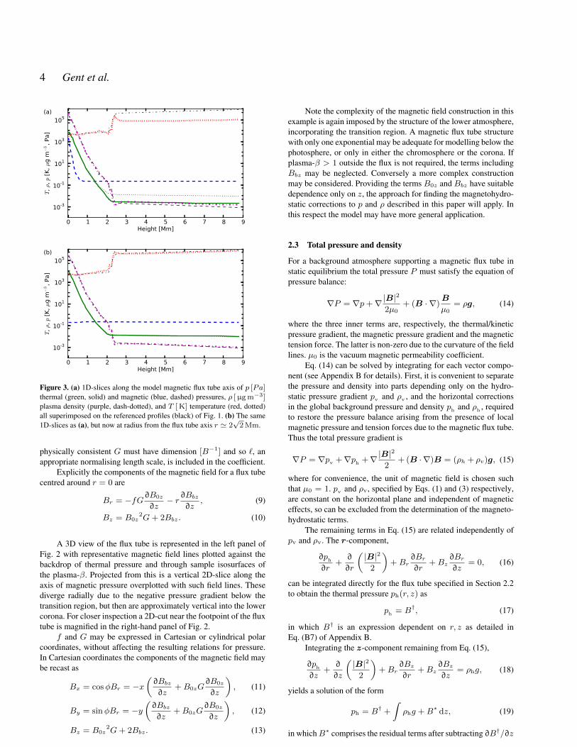
Figure 3. (a) 1D-slices along the model magnetic flux tube axis of p [Pa]thermal (green, solid) and magnetic (blue, dashed) pressures, ρ [µgm−3]plasma density (purple, dash-dotted), and T [ K] temperature (red, dotted)all superimposed on the referenced profiles (black) of Fig. 1. (b) The same1D-slices as (a), but now at radius from the flux tube axis r ' 2
√2Mm.
physically consistent G must have dimension [B−1] and so `, anappropriate normalising length scale, is included in the coefficient.
Explicitly the components of the magnetic field for a flux tubecentred around r = 0 are
Br = −fG∂B0z
∂z− r∂Bbz
∂z, (9)
Bz = B0z2G+ 2Bbz. (10)
A 3D view of the flux tube is represented in the left panel ofFig. 2 with representative magnetic field lines plotted against thebackdrop of thermal pressure and through sample isosurfaces ofthe plasma-β. Projected from this is a vertical 2D-slice along theaxis of magnetic pressure overplotted with such field lines. Thesediverge radially due to the negative pressure gradient below thetransition region, but then are approximately vertical into the lowercorona. For closer inspection a 2D-cut near the footpoint of the fluxtube is magnified in the right-hand panel of Fig. 2.
f and G may be expressed in Cartesian or cylindrical polarcoordinates, without affecting the resulting relations for pressure.In Cartesian coordinates the components of the magnetic field maybe recast as
Bx = cosφBr = −x(∂Bbz∂z
+B0zG∂B0z
∂z
), (11)
By = sinφBr = −y(∂Bbz∂z
+B0zG∂B0z
∂z
), (12)
Bz = B0z2G+ 2Bbz. (13)
Note the complexity of the magnetic field construction in thisexample is again imposed by the structure of the lower atmosphere,incorporating the transition region. A magnetic flux tube structurewith only one exponential may be adequate for modelling below thephotosphere, or only in either the chromosphere or the corona. Ifplasma-β > 1 outside the flux is not required, the terms includingBbz may be neglected. Conversely a more complex constructionmay be considered. Providing the terms B0z and Bbz have suitabledependence only on z, the approach for finding the magnetohydro-static corrections to p and ρ described in this paper will apply. Inthis respect the model may have more general application.
2.3 Total pressure and density
For a background atmosphere supporting a magnetic flux tube instatic equilibrium the total pressure P must satisfy the equation ofpressure balance:
∇P = ∇p+∇|B|2
2µ0+ (B · ∇)B
µ0= ρg, (14)
where the three inner terms are, respectively, the thermal/kineticpressure gradient, the magnetic pressure gradient and the magnetictension force. The latter is non-zero due to the curvature of the fieldlines. µ0 is the vacuum magnetic permeability coefficient.
Eq. (14) can be solved by integrating for each vector compo-nent (see Appendix B for details). First, it is convenient to separatethe pressure and density into parts depending only on the hydro-static pressure gradient pv and ρv , and the horizontal correctionsin the global background pressure and density ph and ρh , requiredto restore the pressure balance arising from the presence of localmagnetic pressure and tension forces due to the magnetic flux tube.Thus the total pressure gradient is
∇P = ∇pv +∇ph +∇|B|2
2+ (B · ∇)B = (ρh + ρv)g, (15)
where for convenience, the unit of magnetic field is chosen suchthat µ0 = 1. pv and ρv, specified by Eqs. (1) and (3) respectively,are constant on the horizontal plane and independent of magneticeffects, so can be excluded from the determination of the magneto-hydrostatic terms.
The remaining terms in Eq. (15) are related independently ofpv and ρv. The r-component,
∂ph
∂r+∂
∂r
(|B|2
2
)+Br
∂Br∂r
+Bz∂Br∂z
= 0, (16)
can be integrated directly for the flux tube specified in Section 2.2to obtain the thermal pressure ph(r, z) as
ph = B†, (17)
in which B† is an expression dependent on r, z as detailed inEq. (B7) of Appendix B.
Integrating the z-component remaining from Eq. (15),
∂ph
∂z+∂
∂z
(|B|2
2
)+Br
∂Bz∂r
+Bz∂Bz∂z
= ρhg, (18)
yields a solution of the form
ph = B† +
∫ρhg +B∗ dz, (19)
in whichB∗ comprises the residual terms after subtracting ∂B†/∂z
Figure 4. Vertical 2D-slice log profile of the magnetohydrostatic background (a) thermal pressure p, (b) density ρ and (c) temperature T . Magnetic field lines(solid, blue) are overplotted in (a) and (b).
0 1 2 3 4 5 6 7 8 9Height [Mm]
10-3
10-1
101
103
105
pla
sma-β
, p [
Pa]
Figure 5. 1D-slices of thermal (green, dashed) and magnetic (blue, dash-dotted) pressures p [Pa], and the plasma-β (red, solid) along the magneticflux tube axis (thick lines) and at axial radius r ' 2
√2Mm (thin lines).
The position of plasma-β = 1 is included (black, dotted) for comparison.
from under the integral. Eq. (19) must equal Eq. (17), requiring∫ρhg +B∗ dz = 0.
This can be satisfied by setting ρh = −g−1B∗, for which B∗ isspecified in Eq. (B10) of Appendix B. The thermal pressure andthe density are now fully specified by
p = pv + ph , ρ = ρv + ρh .
The vertical profiles of the pressure, density and temperaturethus derived are illustrated as 1D-slices in Fig. 3a along the axis ofthe magnetic flux tube and in Fig. 3b outside the flux tube (at radiusr = 2
√2Mm). The axis of the flux tube is slightly over-dense in
the corona, and the temperature is consequently up to an order ofmagnitude lower than the reference data. At the edge of the model
the density and temperature profiles tend to those of the hydrostaticbackground.
The vertical 2D-slices of the pressure, density and temperatureare also displayed in Fig. 4. While a simulation might not extendto a radius exceeding 2Mm, it is included here to confirm that theflux tube remains physically valid beyond the numerical domain.The model has also been checked horizontally to ±5Mm and re-tains the features consistent with the reference data. The horizontalstratification is much weaker than the vertical, so is most apparentin Fig. 4c, because temperature exhibits less vertical stratificationthan plasma pressure or density. The flux tube plasma is cooler thanthe ambient plasma.
In Fig. 5 the variation in plasma-β along the flux tube axis isplotted for the model magnetohydrostatic background along withthe magnetic and thermal pressure profiles. Note, in the corona themagnetic pressure inside and outside the flux tube is similar, butplasma-β . 0.01 along the axis and plasma-β ' 0.05 outsidediffer significantly.
The vertical 2D-slice of the log of plasma-β is also depicted inFig. 6. Note in both illustrations plasma-β > 1 everywhere below1.5Mm, indicating the dominance of thermal pressure, and β < 1everywhere above, indicating the dominance of magnetic pressureeven below the transition region. There is a pronounced kink in thestructure of the plasma-β about z = 2.2Mm, corresponding tothe step in plasma density and temperature at the transition region.Inclusion of these features may help to identify critical transportprocesses in simulations as propagating waves reach the transitionregion.
The 1D-slices of the sound speed cs and Alfven speed vA ofthe magnetohydrostatic background are displayed in Fig. 7. Insideand outside the magnetic flux tube cs is similar below the transi-tion region, but diverges significantly above. vA inside and outsidethe flux tube is quite different below the temperature minimum atz ' 500 km but then is similar after that. In the transition regionthe stepped gradients of cs and vA are very similar to each other,
Figure 6. Vertical 2D-slice of the log magnetohydrostatic backgroundplasma-β; the ratio of thermal to magnetic pressure.
0 1 2 3 4 5 6 7 8 9Height [Mm]
10-2
10-1
100
101
102
103
c s, v A
[km
s−
1]
Figure 7. Vertical 1D-slices of the magnetohydrostatic background soundspeed cs (red) and the Alfven speed vA (blue). Profiles are plotted along themagnetic flux tube axis (solid, dashed) and at axial radius r ' 2
√2Mm
(dash-dotted, dotted).
which may mean Alfven waves could be subject to reflective effectsanalogous to those of sound waves.
2.4 Avoiding negative density and unphysical effects
For our model the axial footpoint strength is 100mT (1000G) atthe photosphere, yielding a full width half maximum (FWHM) ofabout 100 km. This is illustrated in Fig. 8 for z = 3km with a hor-izontal 1D-slice of the magnetic field strength (maximum 70mT)through the flux tube axis. The FWHM of 120 km at z = 3kmis indicated by vertical dotted lines and the half maximum by thehorizontal dotted line. This is large enough to adequately resolvethe profile with a practicable numerical resolution.
The chosen parameters in SI units as identified in this paperare b01 ' 0.7mT, b02 ' 0.01mT, f0 ' 40mTMm, z1 '0.17Mm, z2 ' 175Mm, zb ' 5 · 104 Mm and b00 ' 0.35mT.The scaling length ` ' 8Mm. These parameters must be chosen
Figure 8. Horizontal 1D-slice of the magnetic field strength |B| (solid,blue) through the axis of the magnetic flux tube at z = 3km. Also indicatedare the FWHM, 160 km (vertical, dotted) and the half maximum (magenta,dotted).
to adequately track the total pressure gradient, while generating aplasma-β profile consistent with the physical model.
Our method requires an increase in plasma density inside themagnetic flux tube to balance the magnetic pressure and tensionforces and so the temperature is lower than outside. The meanfootpoint temperature (at z = 3km) within a radius of 50 km isT ' 3600K. This is low compared to observational estimatesnearer to 4000K, however the model is static, while in the solaratmosphere, turbulence may effect the observed temperatures andalso influence the overall pressure balance.
It is important to recognise that ph and ρh may take negativeas well as positive values, subject to the constraints that the sumspv +ph > 0, ρv +ρh > 0 for any location in the domain. It is alsoimportant that they are sufficiently greater than zero, such that theyremain positive and physically consistent even when the dynamicalfluctuations are included during simulations. Note the thermal pres-sure gradient at the transition region exhibits some of the steppedstructure evident in the temperature and density gradients, althoughthe total pressure gradient is relatively smooth.
Within this transition region the plasma-β falls substantiallyso that magnetic pressures predominate. This is where the densityis low and rather sensitive to the strongest perturbations, so it isessential to ensure the background ρ is adequate to contain anylarge negative perturbations.
3 SUMMARY AND DISCUSSION
We have solved analytically the MHD pressure balance equationfor a set of single open vertical magnetic flux tube configurations inmagnetohydrostatic equilibrium within a realistic solar atmosphere,stratified in pressure, plasma density, temperature and magneticfield strength. The solutions are necessarily not inherently simpli-fied, comprising a sum of multiple terms defining the pressure andplasma density functions, and include in this example ten parame-ters. They can, however, be easily coded and visualised. For highperformance computing the functions can also be conveniently par-allelized within numerical simulations.
The arrangement makes it possible to include the challengingstepped gradients in the transition region, rather than a smooth ap-proximation to this profile. The free parameters in the model makeit feasible to adjust the design for numerics in order to handle strong
dynamical fluctuations without obtaining unphysical negativity forpressure or plasma density.
For mathematical transparency the flux tube is an idealisedmodel, without torsion or any axial asymmetry, and the solar atmo-sphere is simplified to exclude local turbulence and fluctuations.However, we have endeavoured to embed the flux tube in a re-alistic gravitationally stratified background atmosphere, matchingclosely the better estimates available from theory and observation.Our model does not critically depend on the prescription of the am-bient magnetic pressure gradient or the precise parametarization ofthe magnetic flux tube, so should data become available this wouldconstrain the model more accurately, but would not invalidate it.
Exploring the magnetohydrostatic states of the model givesan indication for the physical constraints on magnetic field config-uration, pressure, density and temperature, for which equilibriumis valid. It appears from this result, that the over-dense features ofmagnetic flux tubes in the solar corona, may be a natural prereq-uisite to balance the internal and external pressures. With this con-figuration a footpoint strength in excess of 100mT or FWHM forthis footpoint strength in excess of 100 km tend towards inducingregions of negative plasma density or pressure.
Our future work will include applying this analytic fluxtube solution as the background for numerical studies of the en-ergy transport mechanisms between the photosphere and the solarcorona. We expect it to form the basis of a broad suite of such nu-merical models. It is worth explaining the derivation independently,which might otherwise be subsumed in a more general article alsorelating an array of numerical results. The aim of the present pa-per is to make the analytical result available for more general ap-plications, further analysis and to promote the development of themodel. The interactions between multiple flux tubes and alternativeflux tube geometry might be considered, such as torsional or archedtubes.
ACKNOWLEDGEMENTS
FAG is supported by STFC Grant R/131168-11-1. RE is also thank-ful to the NSF, Hungary (OTKA, Ref. No. K83133) and acknowl-edges M. Keray for patient encouragement. The authors would liketo acknowledge the NumPy, SciPy (Jones et al. 2001), Matplotlib(Hunter 2007) and MayaVi2 (Ramachandran & Varoquaux 2011)python projects for providing the computational tools to analysethe data. We thank Andrew Soward for helpful discussion on theMHD equations, Gary Verth for insight into the physical parame-ters of the solar atmosphere and Bernie Roberts on the constructionof the flux tube.
REFERENCES
Aschwanden M. J., 2005, Physics of the Solar Corona. An Intro-duction with Problems and Solutions (2nd edition)
Aschwanden M. J., Schrijver C. J., Alexander D., 2001, ApJ, 550,1036
Deinzer W., 1965, ApJ, 141, 548Fedun V., Erdelyi R., Shelyag S., 2009, SoPh, 258, 219Fedun V., Shelyag S., Erdelyi R., 2011, ApJ, 727, 17Gascoyne A., Jain R., 2009, A&A, 501, 1131Gibson S. E., Low B. C., 1998, ApJ, 493, 460Gordovskyy M., Jain R., 2007, ApJ, 661, 586Hunter J. D., 2007, Computing In Science & Engineering, 9, 90
Table A1. Dimensions of physical quantities used to non-dimensionalisethe numerical equations.
Physics Symbol Dimension Units
Length L [L] 2× 10³ m
Velocity u [u] 103 ms−1
Density ρ [ρ] 10−6 kgm−3
Time t [L]/[u] 2 s
Temperature T [T ] 1 K
Energy Density e [ρ][u]2 1 Jm−3
Magnetic Field B√µ0[ρ]
12 [u] 1.12..× 10−3 T †
Pressure p [ρ][u]2 1 Pa
† µ0 = 4π× 10−7 N A−2
Jones E., Oliphant T., Peterson P., Others, 2001, SciPy: Opensource scientific tools for Python
Khomenko E., Collados M., Felipe T., 2008, SoPh, 251, 589Low B. C., 1980, SoPh, 67, 57Manchester W. B., Gombosi T. I., Roussev I., de Zeeuw D. L.,
Sokolov I. V., Powell K. G., Toth G., Opher M., 2004, Journal ofGeophysical Research (Space Physics), 109, 1102
McWhirter R. W. P., Thonemann P. C., Wilson R., 1975, A&A,40, 63
Priest E. R., 1987, Solar magneto-hydrodynamics.Ramachandran P., Varoquaux G., 2011, Computing in Science &
Engineering, 13, 40Roberts B., Webb A. R., 1978, SoPh, 56, 5Schluter A., Temesvary S., 1958, in Lehnert B., ed., Electromag-
netic Phenomena in Cosmical Physics Vol. 6 of IAU Symposium,The Internal Constitution of Sunspots. p. 263
Schussler M., Rempel M., 2005, A&A, 441, 337Shelyag S., Fedun V., Erdelyi R., 2008, A&A, 486, 655Shelyag S., Fedun V., Keenan F. P., Erdelyi R., Mathioudakis M.,
2011, Annales Geophysicae, 29, 883Shelyag S., Zharkov S., Fedun V., Erdelyi R., Thompson M. J.,
2009, A&A, 501, 735Solanki S. K., Steiner O., 1990, A&A, 234, 519Toth G., 1996, Astrophys. Lett. & Commun., 34, 245Vernazza J. E., Avrett E. H., Loeser R., 1981, ApJS, 45, 635Vigeesh G., Fedun V., Hasan S. S., Erdelyi R., 2012, ApJ, 755, 18Winebarger A. R., Warren H. P., Mariska J. T., 2003, ApJ, 587,
439Zwaan C., 1978, SoPh, 60, 213
APPENDIX A: DIMENSIONAL QUANTITIES
These equations can be non-dimensionalised by dividing the vari-ables with typical units, as detailed in Table A1.
APPENDIX B: SOLUTION TO BACKGROUND STATICEQUILIBRIUM
In this Appendix we explicitly outline the solution to Eqs. (16) and(18).
B1 Basic quantities and derivatives
Listed here are the form of the magnetic field components and thevarious derivatives of the expressions which will be required in the
The magnetic pressure terms will integrate directly in Eq. (14) andso we shall not require the derivatives. They are noted here for in-clusion in the final result.
|B|2
2=
B2r
2+B2z
2
=1
2
(fG
∂B0z
∂z+ r
∂Bbz∂z
)2
+1
2
(B0z
2G+ 2Bbz)2.
B3 Magnetic tension force
The components of the magnetic tension force are given by thegeneral expressions by components r and z, respectively,
Br∂Br∂r
+Bz∂Br∂z
, (B1)
Br∂Bz∂r
+Bz∂Bz∂z
. (B2)
We will require the derivatives in these expressions as follows:
∂Br∂r
= −(B0zG+ f
∂G
∂r
)∂B0z
∂z− ∂Bbz
∂z
= B0zG
(2f2
f02 − 1
)∂B0z
∂z− ∂Bbz
∂z(B3)
∂Br∂z
= −(G∂f
∂z+ f
∂G
∂z
)∂B0z
∂z
−fG ∂
∂z
(∂B0z
∂z
)− r∂
2Bbz∂z2
(B4)
= Gr
(2f2
f02 − 1
)∂B0z
∂z
2
− fG∂2B0z
∂z2− r∂
2Bbz∂z2
∂Bz∂r
= B0z2 ∂G
∂r= −2B0z
3fG
f02 , (B5)
∂Bz∂z
= 2B0zG∂B0z
∂z+B0z
2 ∂G
∂z+ 2
∂Bbz∂z
= 2B0zG
(1− f2
f02
)∂B0z
∂z+ 2
∂Bbz∂z
(B6)
B4 Thermal pressure balancing magnetic field
Having prescribed the magnetic field we now seek to satisfy thepressure balance, first by solving Eq. (16) for the r-components.The first term of the right-hand side below is magnetic pressure.
Subsequent terms yield the expression Eq. (B1) by multiplying Brwith (B3) and Bz with (B4).
∂ph∂r
= −∂
∂r
(|B|2
2
)+((((
((((((((
fG ·B0zG
(2f2
f02− 1
)∂B0z
∂z
2
−fG∂B0z
∂z·∂Bbz
∂z+ r
∂Bbz
∂z·B0zG
(2f2
f02− 1
)∂B0z
∂z
−r∂Bbz
∂z·∂Bbz
∂z−(((
(((((((
((B0z
2G ·Gr(2f2
f02− 1
)∂B0z
∂z
2
+B0z2G · fG
∂2B0z
∂z2− 2Bbz ·Gr
(2f2
f02− 1
)∂B0z
∂z
2
+B0z2G · r
∂2Bbz
∂z2+ 2Bbz · r
∂2Bbz
∂z2+ 2Bbz · fG
∂2B0z
∂z2
. . . = −∂
∂r
(|B|2
2
)+∂
∂r
(2Bbzf
2G
B0z2
+Bbzf0
2G
B0z2
)∂B0z
∂z
2
−Bbzf0
2
B0z
∂G
∂r
∂2B0z
∂z2−B0zf0
2
4
∂G2
∂r
∂2B0z
∂z2
−∂
∂r
(f2G
B0z+���f02G
2B0z
)∂Bbz
∂z
∂B0z
∂z+ 2rBbz
∂2Bbz
∂z2
+���
�����f0
2
2B0z
∂G
∂r
∂Bbz
∂z
∂B0z
∂z−f0
2
2
∂G
∂r
∂2Bbz
∂z2− r
∂Bbz
∂z
2
ph = −|B|2
2+
(2Bbzf
2G
B0z2 +
Bbzf02G
B0z2
)∂B0z
∂z
2
(B7)
−Bbzf02G
B0z
∂2B0z
∂z2− B0zf0
2G2
4
∂2B0z
∂z2− r2
2
∂Bbz∂z
2
−f2G
B0z
∂Bbz∂z
∂B0z
∂z− f0
2G
2
∂2Bbz∂z2
+ r2Bbz∂2Bbz∂z2
.
The solution is constrained by p = pv + ph such that any constantof integration, a function of z, may be expressed within pv. Notethat this solution can be simplified if our model can neglect the am-bient magnetic field Bbz , which outside the flux tube would resultin plasma-β > 1 in the corona and the chromosphere. Then
ph = −|B|2
2− B0zf0
2G2
4
∂2B0z
∂z2(B8)
B5 Plasma density balancing magnetic field
To determine ρh it is also necessary to integrate ∂ph/∂z in Eq. (18).For the magnetic tension terms of Eq. (B2), Br is multiplied withthe expression (B5) and Bz with (B6).
∂ph
∂z= ρhg −
∂
∂z
(|B|2
2
)− r∂Bbz
∂z· 2B0z
3fG
f02 (B9)
−���
������
fG∂B0z
∂z· 2B0z
3fG
f02 −B0z
2G · 2∂Bbz∂z
−B0z2G · 2B0zG
(1−���f2
f02
)∂B0z
∂z
−2Bbz · 2B0zG
(1− f2
f02
)∂B0z
∂z+ 2Bbz · 2
∂Bbz∂z
The solution to this must match that of Eq. (B7). The match can bemore easily identified if we add to this the following list of terms,
If we filter out all of the derivative expressions, which can be in-tegrated directly to return the same result as Eq. (B7) any residualterms must disappear and hence we require
∫dzρhg −
[2B0z
4Gr2
f02
+ 2B0z2G− 4Bbz
]∂Bbz
∂z
+f0
2G
2
∂3Bbz
∂z3+Bbzr
2 ∂3Bbz
∂z3− 2B0z
3G2 ∂B0z
∂z
− 4BbzB0zG
[1−
f2
f02
]∂B0z
∂z+f0
2G
B0z
∂Bbz
∂z
∂2B0z
∂z2
+ fGr∂Bbz
∂z
∂2B0z
∂z2−
3Bbzf02G
B0z2
∂B0z
∂z
∂2B0z
∂z2
+
[f0
2G2
4− f2G2 − 6BbzGr
2
]∂B0z
∂z
∂2B0z
∂z2
−[2f2Gr2
f02
+f0
2G
B0z2+Gr2
]∂Bbz
∂z
∂B0z
∂z
2
+ BbzG
[r2
B0z+
2f02
B0z3+
4fr3
f02
]∂B0z
∂z
3
+B0zf0
2G2
4
∂3B0z
∂z3+Bbzf0
2G
B0z
∂3B0z
∂z3= 0. (B10)
B6 Divergence and pressure balance precision
In cylindrical polar coordinates the divergence of the magnetic fieldis given by
∇ ·B =1
r
∂
∂r(rBr) +
���1
r
∂Bφ∂φ
+∂Bz∂z
(B11)
= −1
r
[∂f
∂zB0zG+ r
∂2f
∂r∂zB0zG+ r
∂f
∂zB0z
∂G
∂f
∂f
∂r
]+
∂f
∂r
∂B0z
∂zG+
∂2f
∂r∂zB0zG+
∂f
∂rB0z
∂G
∂f
∂f
∂z
− 1
r2r∂Bbzz
+ 2∂Bbzz
= 0.
The resulting magnetic field configuration has been checked nu-merically with a mesh resolution δx = 10 km to verify
∇ ·B =∂Bx∂x
+∂By∂y
+∂Bz∂z
= 0.
The resulting error scaled by the local strength of the field has meanof order 10−7, with peak of order 10−4.
The horizontal pressure balance
∂p
∂x+∂
∂x
|B|2
2+Bx
∂Bx∂x
+By∂Bx∂y
+Bz∂Bx∂z
= 0
and vertical pressure balance
∂p
∂z+∂
∂z
|B|2
2+Bx
∂Bz∂x
+By∂Bz∂y
+Bz∂Bz∂z− ρg = 0
have been verified numerically with δx = 10 km for the derivedthermal pressure, density and specified magnetic field configura-tion. For the horizontal pressure balance ε < 10−13 and for thevertical mean relative error ε ' 10−7 with peak of order 10−4. Asδx→ 0 the relative error ε→ 0.
For these and we use the same derivative scheme as appliedin the Versatile Advection Code (Toth 1996) and the Sheffield Ad-vanced Code for MHD (Shelyag et al. 2008), which we plan toemploy for future simulations.