MAGNETOSPHERIC MULTISCALE (MMS) MISSIONATTITUDE GROUND SYSTEM DESIGN

Joseph E. Sedlak, (1) Emil Superfin , (2) and Juan C. Raymond (3)

(1)a.i. solutions, Inc., 10001 Derekwood Lane, Lanham, MD 20706, USA, joseph.sedlak@ai-solutions.com(2)a.i. solutions, Inc., 10001 Derekwood Lane, Lanham, MD 20706, USA, emil.superfin@ai-solutions.com(3)NASA/Goddard Space Flight Center, Code 591, Greenbelt, MD 20771, USA, juan.c.raymond@nasa.gov

Abstract: This paper presents an overview of the attitude ground system (AGS) currently underdevelopment for the Magnetospheric Multiscale (MMS) mission. The primary responsibilities forthe MMS AGS are definitive attitude determination, validation of the onboard attitude filter, andcomputation of certain parameters needed to improve maneuver performance. For these purposes,the ground support utilities include attitude and rate estimation for validation of the onboardestimates, sensor calibration, inertia tensor calibration, accelerometer bias estimation, center ofmass estimation, and production of a definitive attitude history for use by the science teams. Muchof the AGS functionality already exists in utilities used at NASA’s Goddard Space Flight Centerwith support heritage from many other missions, but new utilities are being created specifically forthe MMS mission, such as for the inertia tensor, accelerometer bias, and center of mass estimation.Algorithms and test results for all the major AGS subsystems are presented here.

Keywords: MMS, attitude, ground support

1. Introduction

This paper describes the attitude ground system (AGS) design to be used for support of theMagnetospheric MultiScale (MMS) mission. The AGS exists as one component of the missionoperations control center. It has responsibility for validating the onboard attitude and accelerometerbias estimates, calibrating the attitude sensors and the spacecraft inertia tensor, and generating adefinitive attitude history for use by the science teams.

NASA's Goddard Space Flight Center (GSFC) in Greenbelt, Maryland is responsible fordeveloping the MMS spacecraft, for the overall management of the MMS mission, and for missionoperations. MMS is scheduled for launch in 2014 for a planned two-year mission.

The MMS mission consists of four identical spacecraft flying in a tetrahedral formation in aneccentric Earth orbit. The relatively tight formation, with separations ranging from 10 to 400 km,will provide coordinated observations giving insight into small-scale magnetic field reconnectionprocesses. By varying the size of the tetrahedron and the orbital semi-major axis and eccentricity,and making use of the changing solar phase, this geometry allows for the study of both bow shockand magnetotail plasma physics, including acceleration, reconnection, and turbulence. The missiondivides into two phases for science; these phases will have orbit dimensions of 1.2× 12 Earth radiiin the first phase and 1.2x25 Earth radii in the second in order to study the dayside magnetopauseand the nightside magnetotail, respectively. The orbital periods are roughly one day and three daysfor the two mission phases.

Each of the four MMS spacecraft will be spin stabilized at 3 revolutions per minute (rpm),with the spin axis oriented near the ecliptic north pole but tipped approximately 2.5 deg towards theSun line. The main body of each spacecraft will be an eight-sided platform with diameter of 3.4 mand height of 1.2 m. Several booms are attached to this central core: two axial booms of 14.9 mlength, two radial magnetometer booms of 5 m length, and four radial wire booms of 60 m length.Attitude and orbit control will use a set of axial and radial thrusters. A four-head star tracker (ST)and a slit-type digital Sun sensor (DSS) provide input for attitude determination. In addition, anaccelerometer will be used for closed-loop orbit maneuver control.

This work was supported by the National Aeronautics and Space Administration (NASA)/Goddard Space Flight Center (GSFC),Greenbelt, MD, USA, Contract NNG10CP02C.

22nd International Symposium on Spaceflight Dynamics, INPE, São José dos Campos, SP, Brazil, February 2011.

The primary AGS product will be a daily definitive attitude history. An extended Kalman filter(EKF) will be used to estimate the three-axis attitude (both the spin axis orientation and spin phase)and the rotation rate for all times when the tracker data is available. If there are gaps in the ST data,these will be interpolated, as described in Sec. 2. 1, to create the definitive attitude product.

The four ST heads have separate fields of view that must be calibrated on-orbit to correct forlaunch shift. Section 2.2 describes the alignment calibration for both the ST and the DSS.

To improve the accuracy of the closed-loop orbit maneuver control, the accelerometer biasmust be estimated whenever a burn is planned. Section 2.3 presents the bias estimation algorithmand describes some test cases.

The current MMS spacecraft design does not include rate-sensing gyroscopes, so the EKFmust use dynamical modeling for attitude and rate propagation. One consequence of this is that theaccuracy of the transverse components of the estimated rotation rate is very sensitive to errors inthe inertia tensor. The computed centripetal accelerations are affected by these rate errors; thus, theaccelerometer bias estimation accuracy is affected by the inertia tensor accuracy. Section 2.4 givesa detailed description of the AGS approach to improving the inertia tensor knowledge on-orbit.

Maneuvers on thrusters will impart unintended angular momentum to the spacecraft inproportion to the error in the moment arm of the thrust relative to the center of mass (CM). Toreduce the error in the CM knowledge, the AGS will attempt to estimate the CM position using theDoppler shifts of Global Positioning System (GPS) carrier frequencies. Section 2.5 shows aderivation of the required partial derivatives and gives some very preliminary results.

Concluding remarks are given in Sec. 3.

2. AGS Utilities

This section describes the AGS subsystems needed for MMS support. These include attitudeestimation, validation of the onboard attitude, sensor interference prediction, and several types ofcalibration described below. In addition, the AGS has many other features that include capabilitiessuch as:

• Estimating the attitude by a variety of methods (extended Kalman filter, optimal smoother,or single-frame quaternion estimation (QUEST) [1])

• Generating reference vectors (Sun, Earth, Moon, magnetic field, and guide stars) in thebody frame, the geocentric inertial (GCI) frame, or other special-purpose frames

• Plotting and flagging measurement vectors, attitude solutions, and sensor residuals

• Generating time-dependent visualizations of sensor fields of view (FOV) including stars tomagnitude 9, Sun, Earth, Moon, and planets

• Identifying tracked stars

This wide variety of features puts the AGS at the heart of a powerful ground support system thathas proven invaluable on over two dozen missions for nominal support, calibrations, data analysis,and anomaly resolution.

The AGS was initially created as a general system for three-axis stabilized spacecraft missionsupport [2] and has grown, as needed, by adding capabilities to satisfy specific mission require-ments, including some features for spin-stabilized spacecraft support. The MMS spacecraft arespinners. However, they carry autonomous quaternion-output star trackers, and the attitudeproducts require full three-axis attitudes (not just the spin axis direction). For these reasons, theground system is well served by using a three-axis support system rather than one designed just forspin-stabilized spacecraft. The oldest parts of the AGS were written in FORTRAN in the 1970s and1980s. The generalized multimission version [2] was created in the early 1990s and was used tosupport the UARS, EUVE, and RXTE missions. The AGS was ported to MATLAB in the late-1990s.

2.1. Attitude Sensors and Attitude Products

2.1.1. Attitude Sensors. The MMS spacecraft sensor complement consists of a star tracker (ST)with four separate heads and two redundant digital Sun sensors (DSS) (one being a cold back-upunit). The four ST heads output four independent quaternions at 4 Hz (that is, 16 independentattitude measurements per second). However, the AGS probably will be using telemetry with only a1 Hz data rate (4 attitudes per second). Once per spin period (~20 sec), the DSS will output a pulseindicating sun-crossing through the sensor FOV slit and a measurement of the Sun elevation fromthe body X-Y-plane (the +Z-axis is the nominal spin axis).

All four ST heads are aligned roughly 10 deg offset from the body — Z-axis and are mountedtwo each on two separate stable optical benches. This orientation is a compromise betweenminimizing the star motion through the FOVs and avoiding interference from an axial sensor boomdeployed along the —Z-axis direction. An alignment transformation is applied to the output fromeach ST head so the final output quaternions all represent transformations from the GCI frame tothe body frame.

In addition, there is an acceleration measurement system (AMS) comprising two redundantsets of three orthogonal accelerometers. The AMS is used primarily as part of the closed-loopdelta-V maneuver control system but also can be used in the attitude filter. The centripetalacceleration is proportional to the square of the rotation rate and provides a measure of twocomponents of the rate. The AMS is mounted approximately 0.37 m radially from the spin axis.

2.1.2. Definitive Attitude Products. The AGS currently plans to deliver a definitive attitudeproduct for every orbit of the mission, perigee-to-perigee, after commissioning. The attitudeaccuracy requirement is 0.1 deg (36) per axis for all regions of interest (ROI) to the science team,and best available outside of the ROI. (The ROI usually are near apogee or near perigee, dependingon mission phase.)

It is now expected that ST data will be available for all ROI. However, earlier in the missionplanning, there were power concerns indicating that the ST could only be powered on for perhaps10 percent of each orbit. That led us to design the AGS to allow for partial data coverage.

For all time spans with valid ST data, the AGS will generate attitude and rate solutions usingan EKF, discussed below. If there are gaps in the data, these will be bridged by assuming theangular momentum is constant in both the GCI and body frames. The resulting attitude history isthe definitive attitude. When filling any data gaps, the major principal axis of inertia is aligned withthe angular momentum direction (e.g., the mean angular momentum estimated from the data setsbefore and after the gap). The spin phase in the gaps is computed using the DSS Sun pulses tomaintain synchronization. If there also is a gap in DSS data due to eclipse, the spin phase will beinterpolated using a constant rate from the last DSS Sun pulse of one data set to the first Sun pulseof the next data set, or extrapolated using the mean rate determined by the EKF.

With this approach, the resulting attitude solutions in the data gaps do account for coning(misalignment of the major principal axis from the body Z-axis), but not for nutation (offset of theangular momentum vector in the body frame from the major principal axis). Any nutation isexpected to be damped to an amplitude less than 0.1 deg, except possibly for orbits followingmaneuvers, so this is not a concern.

2. 1.2. 1. Kalman Filter. The spinning spacecraft EKF used in the AGS, referred to here as SpinKF,is the SpinKF-I described in [3]. This filter is conceptually similar to the “standard” Lefferts,Markley, and Shuster quaternion and rate filter described in [4]; however, the SpinKF state vectoravoids using the quaternion. Instead, the SpinKF uses a seven-parameter angular-momentum-basedrepresentation [5]. The seven state vector elements are the angular momentum components in theGCI frame, the angular momentum components in the spacecraft’s body frame, and a spin phaseangle. These parameters are subject to the constraint that the magnitude of the angular momentum

3

is the same in the inertial and body frames (just as the standard quaternion and rate filter has sevenstate components with the constraint that the quaternion be normalized).

The value of the angular-momentum-based representation is improved numerical accuracy.Most spinning spacecraft do not carry rate-sensing gyros; thus, the Kalman filter for a spinnerusually must integrate the dynamics equations to propagate the state between observations. Thisnumerical integration is more accurate for a set of parameters having less variation. For spinningspacecraft, all four quaternion components are rapidly varying. The angular-momentum-basedrepresentation has only a single rapidly varying component; that is the spin phase, and it isincreasing only linearly (mod 27c) rather than varying sinusoidally.

The SpinKF algorithm has been used operationally for the ST-5 and THEMIS missions. It hasbeen tested for MMS with several scenarios using a simple simulator and also with a high-fidelitysimulation including oscillations of the flexible wire booms and other appendages. The attitudeestimation error has been found to be well under the required 0.1 deg (3 6) tolerance. Typical 3 6

errors are roughly 0.05 deg about the Z-axis and 0.02 deg about X and Y.

2.1.2.2. Attitude Validation. To validate the performance of the onboard EKF, the SpinKF attitudewill be compared with the onboard attitude estimate for a time span of roughly two hours each day(the actual time span is yet to be negotiated). The mean and standard deviation of this attituderesidual will be reported to the mission operations center (MOC).

In addition, SpinKF statistics for the attitude, rate, and individual sensor residuals will besaved in a trending database. This database serves two important purposes: it allows the AGS teamto spot early signs of sensor degradation, and it shows how fast the angular momentum isprecessing in the GCI frame due to environmental torques.

2.1.3. Predicted Attitude Products. Using the most recent definitive attitude product forinitialization, an attitude prediction will be generated periodically. Early in the mission, thisprediction will be created by assuming the major principal axis of inertia is aligned with the angularmomentum vector, which is assumed constant in GCI. As trending data accumulates, it may proveuseful to include a simple empirical model of the daily spin axis drift. This drift is caused by acombination of gravity gradient, drag, and solar pressure torques, but these torques will not bemodeled explicitly. It is expected that the drift will be less than 0.01 degrees per day.

The predicted attitude will be used for two purposes. First, it will indicate when the nextattitude maneuver is needed to maintain the correct spin axis orientation with respect to the Sun andecliptic pole. This maneuver will be scheduled roughly every two weeks. Second, the predictionswill be used to indicate when to expect Earth or Moon interference in the ST or DSS. Since the spinphase cannot be predicted, the interference report will not tell which ST head is occulted versustime, but it will indicate the fraction of each spin period subject to interference for each head.

2.2. Attitude Sensor Alignment Calibration

Early in the commissioning phase of the MMS mission, the ST and DSS will be calibrated foralignment. It is possible that the seasonal variation of the solar beta angle will cause thermalvariations that affect the alignments. If these prove to be significant, then the alignment calibrationsmay be repeated, as needed. It must be emphasized that in-flight calibration can only correct forrelative misalignment and not for absolute alignments in the body frame. In effect, the meanalignment of the four ST heads defines the body frame on orbit.

2.2.1. ST Alignment Calibration. The four ST heads are located pair-wise on two opticalbenches. Their prelaunch alignments will be measured by optical methods using reflective cubes onthe benches. Alignment calibration is performed on-orbit to correct for any shift due to launchshock, release of gravitational stress, and change of thermal environment.

4

The relative alignment of two heads on the same bench is likely to remain more stable thantwo heads on separate benches. (This will be monitored as trending data is collected throughout themission.) Nonetheless, the relative alignments of all four heads will be determined after launch.

The AGS calibration utility will use the ALIQUEST method [6]. This attitude-dependentmethod solves for the misalignment using a reference attitude and is based on the QUESTquaternion estimation algorithm [1]. The QUEST algorithm is a well-known, efficient, and reliablemethod to determine the attitude by minimizing the loss function, L, as a function of the attitudematrix, A,

L(A) = ∑[vi ody − Avi

ref ] 2 (1)

i

where vector vibody is the observation unit vector for sensor i expressed in the body frame, viref is the

corresponding inertial frame reference vector, and index i runs over all sensors available at a giventime. The matrix A is the “single-frame” attitude estimate at that time. Similarly, the attitude-dependent alignment estimation problem can be cast in a parallel form. That is, determine themisalignment for a given sensor by minimizing the loss function

L(O) = ∑[O &dy − Ajv r of ]

2

(2)j

j

as a function of the orthogonal misalignment matrix, O, where subscript j is a time index runningover all valid observations, and Aj is the known attitude history. The vector vj body is the observationunit vector for the given sensor, rotated to the body frame using the nominal alignment, No, and anya priori misalignment, Mo . Once O is determined, the new misalignment is usually expressed in thesensor frame as

M = No

− 1 ONoM

o , (3)

where the inverse of No is used here rather than the matrix transpose to allow for possiblenonorthogonality. It is clear Eqs. 1 and 2 can be minimized using the same method. Choosing theQUEST algorithm [1] to solve Eq. 2 results in the ALIQUEST utility.

For the MMS ST calibration, the reference attitude will be generated using approximately thesame number of pre-calibration observations from each ST head, all with the same weight. Thismakes the reference attitude, in effect, an average over all four misalignments. After the calibration,the alignments of the four ST heads will have been adjusted to agree with this reference attitude.Thus, when the calibrated ST data is used in an attitude filter, the ST residuals will be reduced butthe attitude solution should be unchanged. This means that ALIQUEST calibrations can beperformed at any time during the mission without introducing any discontinuity in the definitiveattitude histories being delivered daily to the science teams.

2.2.2. DSS Alignment Calibration. While the four ST heads provide almost all of the dataneeded by the SpinKF attitude filter, the DSS also contributes some attitude and rate information.The DSS contribution is much smaller than that of the ST since it is available only once per spinand its intrinsic errors are larger than those of the ST. Nonetheless, if the DSS is misaligned withrespect to the ST, its use in the filter can actually make the solutions worse. Thus, it is important tocalibrate the alignment of the DSS relative to the ST early in the mission.

The ST head alignment will be performed first, as described above. This assures that an ST-based attitude solution will be the best available as a reference attitude. The ALIQUEST utility willuse this reference attitude to determine the mean systematic error in the DSS data.

The only difference between the DSS and ST calibrations is that the DSS alignment is notobservable about the Sun vector. The Sun vector measurement in the body frame will be nearlyconstant over the entire calibration data set. (It can be exactly constant if all Sun measurements fallwithin the same digitization bin.) This can cause the ALIQUEST alignment correction matrix to

5

have a large error about the axis corresponding to the Sun direction [6]. To avoid this problem, thecorrection matrix is expressed as three Euler angles, with the third Euler axis along the Sundirection. To remove the error, the final correction matrix is composed of just the first two Eulerangles, with the third angle set to zero. This is equivalent to representing the DSS correction as anazimuthal rotation of the detection slit and an elevation rotation along the direction of the slit.

2.3. Accelerometer Calibration

During the AGS design process, it was decided that two different accelerometer calibrationsmay be necessary to meet orbit maneuver requirements. The two calibration parameters are biasand scale factor. At the time of this paper’s writing, only bias estimation has been prototyped andtested. The actual need for scale factor calibration is still under study.

The accelerometer is used for onboard, closed-loop, delta-V maneuver control. The AGS istasked with determining the accelerometer bias prior to each maneuver. The required accuracy formaneuver support is 2 µg (3 σ) per axis.

The filter for the accelerometer bias works in conjunction with the attitude and rate filter. Thiscombination is a type of “cascaded” filter. This name comes from the way in which both filters runsimultaneously, but information flows only in one direction − from the attitude and rate filter to thebias filter.

The bias filter is designed as a standard EKF with a 3-element state vector representing theaccelerometer bias for each axis. The measurement residual is

racc = kbs − dest , (4)

where a

obs is the accelerometer observation, and where the estimated measurement is

aest = dt × Racc + ω; (−) × (ω; (−) × R

acc )+ b; (−) , (5)

using the dynamics equation

dw = J− 1

(LB

× w; (−) + f) , (6)dt

and where the angular momentum in the body frame is

LB = Jω

; (−) . (7)

The vector kcc runs from the center of mass to the accelerometer and is given in meters, ω ; (−) is

the a priori rate estimate (taken from the attitude and rate filter) at time ti in rad/sec, b; (−) is thea priori bias estimate at time ti in m/sec2, and f is the torque expressed in the body frame, whichcould be calculated from thruster data (however this bias filter is expected to be run only prior tomaneuvers and not during the actual burns, so f will generally be zero).

The partial derivative of Eq. 4 with respect to the bias error yields the sensitivity matrix neededby the EKF,

H = I 3 , (8)

where I3 is the 3 ×3 identity matrix.

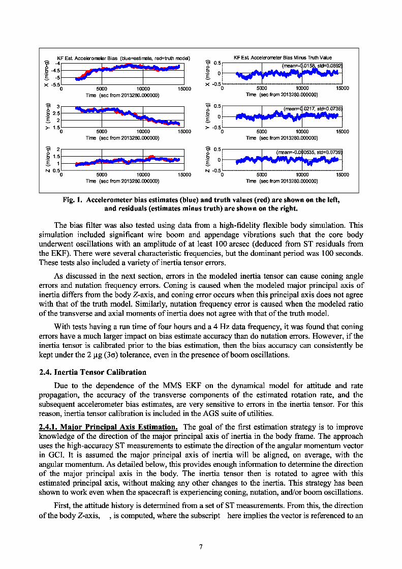
The bias filter was tested first using a set of rigid body simulation data. The results of a samplerun are shown in Fig. 1. It was found in all tests that the filter could predict the bias to within0.9 µg (3 σ) per axis, with a run time of four hours and observations at 4 Hz.

6

KF Est. Accelerometer Bias (blue=estimate, red=truth model)rn -4

-4.5E -5

X -5.50 5000 10000 15000

Time (sec from 2013280.000000)

3°b 2.5

E 2

r 1.50 5000 10000 15000

Time (sec from 2013280.000000)

rn 2

b 1.5E 1N 0.5

0 5000 10000 15000Time (sec from 2013280.000000)

KF Est. Accelerometer Bias Minus Truth Value

0.5 (mean=-0.0158, std=0.0892)00E

X -0.5

0 5000 10000 15000Time (sec from 2013280.000000)

o, 0.50 (mean=0.0217, std=0.0736)

0E

> -0.5

0 5000 10000 15000Time (sec from 2013280.000000)

0.5b (mean=-0.000535, std=0.0739)

0E

N -0.5

0 5000 10000 15000Time (sec from 2013280.000000)

Fig. 1. Accelerometer bias estimates (blue) and truth values (red) are shown on the left,and residuals (estimates minus truth) are shown on the right.

The bias filter was also tested using data from a high-fidelity flexible body simulation. Thissimulation included significant wire boom and appendage vibrations such that the core bodyunderwent oscillations with an amplitude of at least 100 arcsec (deduced from ST residuals fromthe EKF). There were several characteristic frequencies, but the dominant period was 100 seconds.These tests also included a variety of inertia tensor errors.

As discussed in the next section, errors in the modeled inertia tensor can cause coning angleerrors and nutation frequency errors. Coning is caused when the modeled major principal axis ofinertia differs from the body Z-axis, and coning error occurs when this principal axis does not agreewith that of the truth model. Similarly, nutation frequency error is caused when the modeled ratioof the transverse and axial moments of inertia does not agree with that of the truth model.

With tests having a run time of four hours and a 4 Hz data frequency, it was found that coningerrors have a much larger impact on bias estimate accuracy than do nutation errors. However, if theinertia tensor is calibrated prior to the bias estimation, then the bias accuracy can consistently bekept under the 2 µg (3σ) tolerance, even in the presence of boom oscillations.

2.4. Inertia Tensor Calibration

Due to the dependence of the MMS EKF on the dynamical model for attitude and ratepropagation, the accuracy of the transverse components of the estimated rotation rate, and thesubsequent accelerometer bias estimates, are very sensitive to errors in the inertia tensor. For thisreason, inertia tensor calibration is included in the AGS suite of utilities.

2.4.1. Major Principal Axis Estimation. The goal of the first estimation strategy is to improveknowledge of the direction of the major principal axis of inertia in the body frame. The approachuses the high-accuracy ST measurements to estimate the direction of the angular momentum vectorin GCI. It is assumed the major principal axis of inertia will be aligned, on average, with theangular momentum. As detailed below, this provides enough information to determine the directionof the major principal axis in the body. The inertia tensor then is rotated to agree with thisestimated principal axis, without making any other changes to the inertia. This strategy has beenshown to work even when the spacecraft is experiencing coning, nutation, and/or boom oscillations.

First, the attitude history is determined from a set of ST measurements. From this, the directionof the body Z-axis, , is computed, where the subscript here implies the vector is referenced to an

inertial reference frame, and the caret indicates unit vector. The angular momentum direction, ,may be found by calculating the vector around which the Z-axis rotates in inertial space. If there isno nutation, then will rotate around on a circular cone. If there is nutation then the motion willbe more complicated as will rotate around the major principal axis, , which itself will berotating around . Given enough data and an integral number of nutation periods, may be foundin either case by taking the time-average of the motion of .

Next, this estimate of the angular momentum direction is converted to the body frame usingthe known attitude history to yield a set of unit vectors, , where the subscript here implies thevector is referenced to the body frame. Then, is averaged over the entire span of nutationperiods and re-unitized to obtain , where the overbar indicates the mean value.

If there is no nutation, all the vectors will be parallel (to within the attitude noise) andnearly equal to . If there is nutation, will sweep out an elliptical cone around in the bodyframe. In either case, the major principal axis in the body frame, , is approximated by .

Finally, the utility computes the direction cosine matrix (DCM) [7] that rotates the a priorimajor principal axis, , into . This DCM is used in a similarity transform on the a prioriinertia tensor, Jprior , to yield a new tensor whose major principal axis is the one estimated. That is,

(9)

(10)

(11)

(12)

where the caret indicates unit vector and where is the skew-symmetric cross-product operator

(13)

Performing this estimation does not give any information about the directions of the inertiatensor’s two transverse principal axes. By using a minimal rotation, M, from the a priori principalaxis to , the original directions of the transverse principal axes are affected very little.

The reference attitude for this calibration comes from the EKF solution (although raw STattitudes could be used). If the EKF is used, there will be some dependence on the a priori inertiatensor. Once a new tensor is obtained from Eq. 12, the filter can be rerun and the process iterated.Convergence has been found to be very rapid; two or three iterations typically are sufficient todetermine the principal axis to within less than an arc-second.

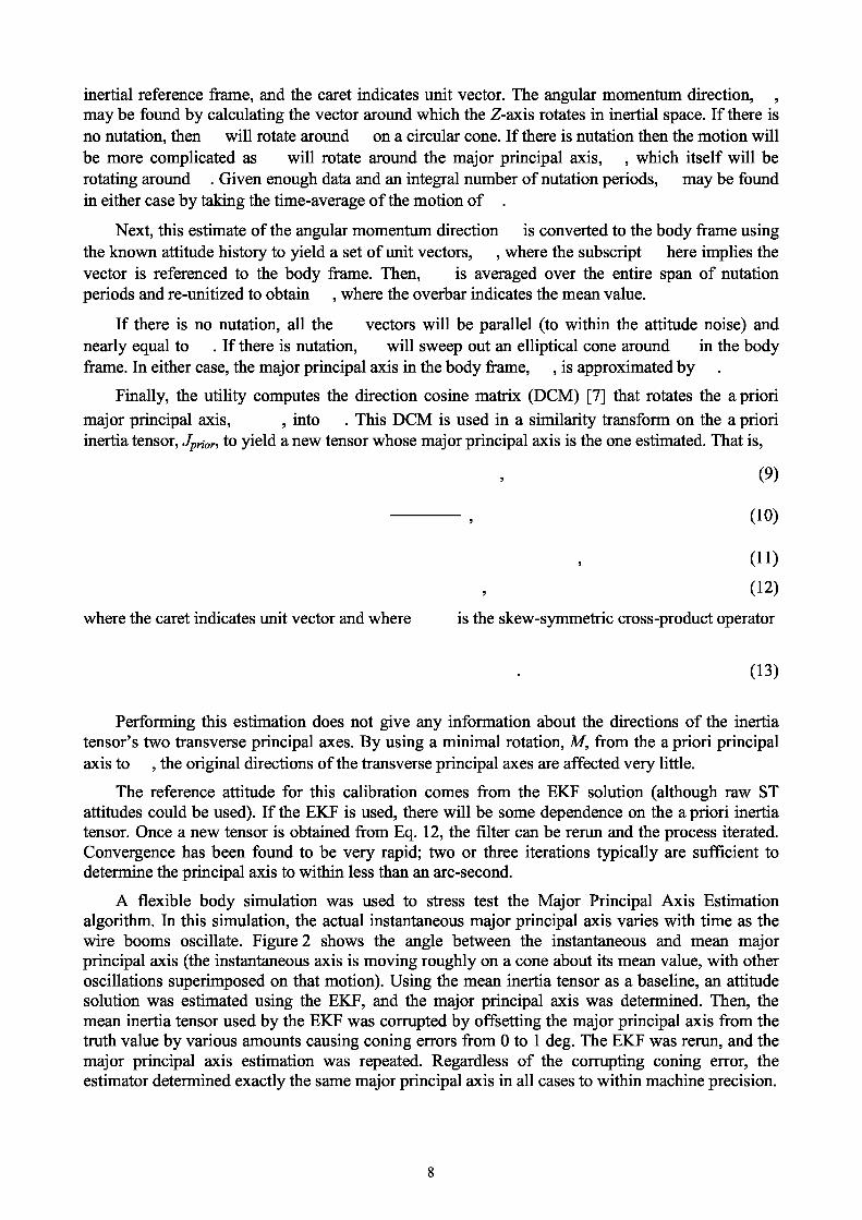
A flexible body simulation was used to stress test the Major Principal Axis Estimationalgorithm. In this simulation, the actual instantaneous major principal axis varies with time as thewire booms oscillate. Figure 2 shows the angle between the instantaneous and mean majorprincipal axis (the instantaneous axis is moving roughly on a cone about its mean value, with otheroscillations superimposed on that motion). Using the mean inertia tensor as a baseline, an attitudesolution was estimated using the EKF, and the major principal axis was determined. Then, themean inertia tensor used by the EKF was corrupted by offsetting the major principal axis from thetruth value by various amounts causing coning errors from 0 to 1 deg. The EKF was rerun, and themajor principal axis estimation was repeated. Regardless of the corrupting coning error, theestimator determined exactly the same major principal axis in all cases to within machine precision.

8

The reproducibility of the estimate to machine precision of course should not be taken as theultimate accuracy of the method. While that accuracy holds for test corruptions in a given specificdata set, results will actually vary slightly from data set to data set due to real world variations inthe ST noise, the boom oscillations, and in the true inertia tensor itself. However, due to theaveraging steps in the algorithm, the actual accuracy can be expected to be significantly better thanthe attitude accuracy of 0.1 deg.

Angle between Instantaneous and Mean Major Principal Axis0.35

0.3

0.25

0.2

(D

0.15Q

0.1

0.05

00 100 200 300 400 500 600 700 800

Time (sec)

Fig. 2. Angle between instantaneous and mean major principal axis for inertia tensor calibration test.

2.4.2. Inertia Ratio Estimation. The goal of the second estimation strategy is to improveknowledge of the spacecraft nutation frequency by estimating the ratio of the transverse and axialmoments of inertia. This method finds the dominant frequencies in the evolution of two geometricparameters. The ratio of these frequencies yields the ratio of the moments of inertia. Before usingthis algorithm, it is assumed the Major Principal Axis Estimator described above has already beenapplied to the inertia tensor.

Since it is based on ratios of measured frequencies, the Inertia Ratio Estimation algorithmdescribed here is not expected to work well when flexible modes are significant. For this reason, itis planned to use this part of the inertia calibration utility only prior to deployment of the flexiblebooms, when the spacecraft can still be considered approximately a rigid body. As such, its valuewill be in validating the ground-based mechanical model of the inertia tensor for the fully stowedconfiguration and again after deployment of the rigid magnetometer boom.

For the case of a nutating cylindrical spacecraft, the following relations hold [8]:

(14)

(15)

where, is the instantaneous rotation rate, is the body nutation rate, is the inertial nutationrate, is the moment of inertia about the i-th principal axis, and is the nutation angle. For a non-axisymmetric spacecraft, we use the average of the transverse moments of inertia in place of .

Figure 3 (based on a diagram in [8]) shows a view looking down onto the plane perpendicularto the angular momentum vector and shows the relationships among the various rates and bodyvectors as they move in the GCI frame. In this figure, it is assumed the nutation angle is small.

Ultimately, the goal is to correct the inertia tensor based on the ratio in Eq. 15. To do this, it isnecessary first to estimate and . By inspection of Fig. 3, it is seen that can be determinedby taking the Fourier transform of the X- or Y-component of the major principal axis, , in aninertial frame perpendicular to the angular momentum vector (that is, in the plane shown in Fig. 3).To estimate , the Fourier transform of the angle between the reference R and the angularmomentum vector should be examined. Figure 4 shows this relationship as a 3-dimensional plotwhere it is clear that this angle’s magnitude will oscillate at the body nutation rate, . It isconvenient to take vector to be the body Z-axis.

Fig. 3. Motion in GCI frame of the principal axis and an arbitrary reference vector (constant inthe body frame) for a nutating spacecraft. The plot is centered on the angular momentum L,

and is the projection of onto the plane perpendicular to L.

Fig. 4. Motion of principal axis P and arbitrary reference axis R showing nutation.

Once and are found, Eq. 15 is used, with the small nutation angle assumption, tocalculate . The inertia tensor’s largest eigenvalue is then changed to the new . Note thatmodifying and not the transverse moments is an arbitrary choice. The overall scaling of theinertia tensor is not determined by these methods; however, that scaling is only relevant in thepresence of external torques and is not needed for improving the nutation modeling.

A set of rigid body simulations was run to test the Inertia Ratio Estimation algorithm. Theinertia tensor was corrupted by changing the inertia ratio by 33 percent, causing a large error in thepredicted nutation. The EKF used this corrupted inertia tensor to estimate the attitude. Then, theInertia Ratio Estimation utility used this attitude to compute the parameters described above before

10

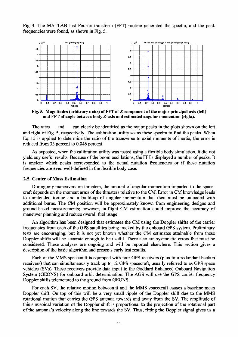
Fig. 3. The MATLAB fast Fourier transform (FFT) routine generated the spectra, and the peakfrequencies were found, as shown in Fig. 5.

x 10-3 FFT of Principal Axis x 10

-3 FFT of angle between Z-axis and mean of Z-axis

4.5

43.5

3.53

32.5

2.5

22

1.5 1.5

1 1

0.5 0.5

0 0.1 0.2 0.3 0.4 0.5 0.6 0.7 0.8 0.9 1 0 0.1 0.2 0.3 0.4 0.5 0.6 0.7 0.8 0.9 1rad/sec rad/sec

Fig. 5. Magnitudes (arbitrary units) of FFT of X-component of the major principal axis (left)and FFT of angle between body Z-axis and estimated angular momentum (right).

The rates and can clearly be identified as the major peaks in the plots shown on the leftand right of Fig. 5, respectively. The calibration utility scans these spectra to find the peaks. WhenEq. 15 is applied to determine the ratio of the transverse to axial moments of inertia, the error isreduced from 33 percent to 0.046 percent.

As expected, when the calibration utility was tested using a flexible body simulation, it did notyield any useful results. Because of the boom oscillations, the FFTs displayed a number of peaks. Itis unclear which peaks corresponded to the actual nutation frequencies or if these nutationfrequencies are even well-defined in the flexible body case.

2.5. Center of Mass Estimation

During any maneuvers on thrusters, the amount of angular momentum imparted to the space-craft depends on the moment arms of the thrusters relative to the CM. Error in CM knowledge leadsto unintended torque and a build-up of angular momentum that then must be unloaded withadditional burns. The CM position will be approximately known from engineering designs andground-based measurements; however, in-flight CM estimation could improve the accuracy ofmaneuver planning and reduce overall fuel usage.

An algorithm has been designed that estimates the CM using the Doppler shifts of the carrierfrequencies from each of the GPS satellites being tracked by the onboard GPS system. Preliminarytests are encouraging, but it is not yet known whether the CM estimates attainable from theseDoppler shifts will be accurate enough to be useful. There also are systematic errors that must beconsidered. These analyses are ongoing and will be reported elsewhere. This section gives adescription of the basic algorithm and presents early test results.

Each of the MMS spacecraft is equipped with four GPS receivers (plus four redundant backupreceivers) that can simultaneously track up to 12 GPS spacecraft, usually referred to as GPS spacevehicles (SVs). These receivers provide data input to the Goddard Enhanced Onboard NavigationSystem (GEONS) for onboard orbit determination. The AGS will use the GPS carrier frequencyDoppler shifts telemetered to the ground from GEONS.

For each SV, the relative motion between it and the MMS spacecraft causes a baseline meanDoppler shift. On top of this will be a very small ripple of the Doppler shift due to the MMSrotational motion that carries the GPS antenna towards and away from the SV. The amplitude ofthis sinusoidal variation of the Doppler shift is proportional to the projection of the rotational partof the antenna’s velocity along the line towards the SV. Thus, fitting the Doppler signal gives us a

11

measurement of that velocity component, which in turn is proportional to the spin rate times thevector from the true CM to the antenna. The difference between this measurement and theprediction based on the nominal CM will be filtered to give the offset of the true CM from itsnominal position. The attitude and all the orbits are known, so the geometric parts of themeasurement model are all fully determined except for the CM offset error.

The four GPS antennas are located roughly 1.6 meter from the spin axis and every 90 deg inazimuth. As MMS rotates, the tracked SVs are handed off from one GPS antenna to the next. Thus,there is good observability of the CM in the body X-Y-plane. However, there is no observability ofthe CM component along the spin axis. The Z-component possibly will have some limitedobservability during orbits after maneuvers when there is significant nutation.

The MMS and GPS SV ephemerides provide the position and velocity vectors of the space-craft CMs in the GCI frame, , , , and . Denote the n-th GPS antenna location inthe MMS body frame as . The nominal CM location in the MMS body frame is , which isused as the a priori guess for the estimator. The true CM body frame position vector is denotedand its estimate is . The GCI position and velocity of the n-th antenna are

(16)and

(17)

where

, (18)

and where the transpose of the attitude matrix, A T, transforms vectors from the body frame to theGCI frame.

For simplicity, define the following body frame and GCI frame vector differences

(19)and

. (20)

Then, the position and velocity of the GPS spacecraft relative to the n-th antenna, expressed in thebody frame, are

(21)

and

(22)

With these definitions, the Doppler shift can be written as

(23)

where . In the nonrelativistic limit, γ is set to unity and the vector additions inEqs. 21 and 22 do not make use of the Lorentz transformation. (Further analysis will be done toverify whether this approximation is justified.) The fractional Doppler shift, D, is defined to be

— . (24)

12

The quantity D is the effective measurement for the CM estimator. It must be expanded in .Using the notation for the cross-product operator, defined as in Eq. 13, the inner product inthe numerator of Eq. 24 is

(25)

The denominator of Eq. 24 can be expanded as

(26)

where ΔR is the magnitude of . The fractional Doppler shift now can be expanded as

(27)

The sensitivity matrix, H, is the partial derivative of the observation with respect to the statevector . That is,

(28)

Note that one minus sign comes from the partial derivative of Eq. 18, . The Hmatrix is used in a recursive least-squares estimator [8] to determine the value of from a set ofD measurements.

If one is solving for all three components of the CM position, then Eq. 28 gives the appropriatesensitivity matrix. However, the Z-component of the CM has very poor observability due to the

term, and it may be preferred to solve only for the X- and Y-components. In this case, thesensitivity matrix is

(29)

The probable number of GPS SVs that will be tracked by the MMS onboard navigation systemvaries with orbital position. The number peaks at perigee, and drops rapidly as MMS moves abovethe GPS constellation. For testing, it was assumed that an average of seven SVs were tracked forsix hours centered on the MMS perigee. The data rate was taken to be 1 Hz. (This rate is the sameas the onboard single-point GPS solutions, but it is not yet known if this rate will be available intelemetry for AGS use.) The noise on the measured fractional Doppler shift D was taken to be zero-mean, white, and Gaussian-distributed with a standard deviation of 10 -9. The modeled CM offseterrors were 4 cm on X and –4 cm on Y. Figure 6 shows a typical result for the X-axis CM estimateunder these test conditions (the Y-axis is similar). At the end of the run, the X estimate is 3.51 cmand the Y estimate is –4.10 cm. The test accuracies are consistent with the errors from the estimatedcovariance matrix, shown as error bounds in Fig. 6.

3. Conclusions

The AGS suite of utilities has been prototyped, tested, and shown ready to meet thechallenging MMS mission requirements. For its primary attitude and rate estimator, the AGS will

13

use the SpinKF version of the attitude Kalman filter [3]. This filter has been thoroughly testedduring support for the ST-5 and THEMIS missions. The AGS will create a daily definitive attitudehistory using batches of star tracker data with SpinKF. If there are data gaps, these will be inter-polated by assuming a constant angular momentum direction and using DSS data to determine thespin phase. This approach has been shown to be feasible to meet the MMS mission requirementsfor attitude and rate estimation.

Estimate of r = 3.51 cmcm,X

8

6

EU

X 4

U 2

00 2 4 6 8 10 12 14 16

Observation # X 10 4

Fig. 6. Recursive least-squares estimate of X-axis CM offset and 16 error bounds. Truth value is 4 cm.

The AGS calibration utilities include algorithms for the estimation of sensor alignments,inertia tensor, accelerometer bias, and CM offset. Since the MMS ST has four separate heads, it isconvenient to use an attitude-dependent method for estimating the relative alignments [6]. This willbe the first AGS calibration performed on-orbit. It may be repeated periodically to ascertainwhether seasonal thermal variations affect the alignments, in particular between the two opticalbenches. The second calibration to be performed will be the inertia tensor estimation. Improvedknowledge of the inertia tensor leads to improved rate estimation because the SpinKF mustpropagate the state between observations using the dynamics equations. Improved rates lead toimproved centripetal acceleration prediction (Eqs. 5 and 6), which in turn yields a more accurateaccelerometer bias estimation. The bias calibration will be performed prior to every burn.

The AGS team is studying the possibility of estimating the CM on-orbit. This is an importantparameter needed for accurate orbit maneuver control. Any error in the CM knowledge leads toerrors in the predicted torques during burns, leading to angular momentum build-up. This wouldnecessitate additional thruster firings to unload the excess angular momentum. This paper describesan approach to CM estimation using the raw Doppler shifts of the carrier frequencies from the GPSsatellites being tracked by the onboard GPS system. Preliminary results have been very positivealthough systematic errors have not yet been considered, and the quantity and quality of theavailable data is still under investigation. As an alternative CM estimation method, the AGS team isactively investigating the possibility of combining accelerometer measurements and onboard GPSpoint-solutions in either a Kalman filter or a least-squares method.

The AGS suite of utilities has been shown to satisfy the MMS mission requirements, ascurrently defined. The AGS heritage of use on a wide variety of past missions has demonstrated itscapabilities for attitude and calibration support. In addition, the AGS has proven invaluable forattitude-related anomaly resolution on many missions. The new utilities designed for MMS have allbeen prototyped and have passed preliminary tests. With a robust design and prototypes in hand,the AGS team is ready to move on to formal development and testing and will be ready to supportmission rehearsals and launch over the next few years.

14

4. References

[ 1 ] Shuster, M. D. and Oh, S. D., “Three-Axis Attitude Determination from Vector Observations,”J. Guidance and Control, Vol. 4, No. 1, Jan.-Feb. 1981, pp. 70-77.

[2] Langston, J., et al., “A Multimission Three-Axis Stabilized Spacecraft Flight DynamicsGround Support System,” 1992 Flight Mechanics/Estimation Theory Symposium, NASAConference Publications CP-3186, NASA/GSFC, Greenbelt, MD, May, 1992.

[3] Markley, F. L. and Sedlak, J. E., “Kalman Filter for Spinning Spacecraft Attitude Estimation,”Journal of Guidance, Control, and Dynamics, Vol. 31, No. 6, p. 1750, Nov-Dec 2008.

[4] Lefferts, E. J., Markley, F. L., and Shuster, M. D., “Kalman Filtering for Spacecraft AttitudeEstimation,” Journal of Guidance, Control, and Dynamics, Vol. 5, No. 5, pp. 417–429, 1982.

[5] Markley, F. L., “New Dynamic Variables for Momentum-Bias Spacecraft,” The Journal of theAstronautical Sciences, Vol. 41, No. 4, pp. 557–567, 1993.

[6] Hashmall, J. A. and Sedlak, J. E., “New Attitude Sensor Alignment Calibration Algorithms,”53rd Int. Astronautical Congress, IAC-02-A.4.07, IAF, Houston, TX, Oct. 2002.

[7] Shuster, M. D., “A Survey of Attitude Representations,” Journal of the Astronautical Sciences,Vol. 41, No. 4, Oct.-Dec., 1993, pp. 439-517.

[8] Wertz, J. R., (ed.), Spacecraft Attitude Determination and Control, D. Reidel PublishingCompany, Dordrecht, The Netherlands, 1978.

15