MAHARAVO RANDRIANARIVONY - xdomitri.com · The wavelet bases are constructed on the unit square...

MULTIWAVELET BOUNDARY ELEMENT METHOD FOR

CAVITIES ADMITTING MANY NURBS PATCHES

MAHARAVO RANDRIANARIVONY

Abstract. We consider the modeling and simulation by means of multiwavelets on

many patches. Our focus is on molecular surfaces which are represented in the form

of Solvent Excluded Surfaces that are featured by smooth blendings between the con-

stituting atoms. The wavelet bases are constructed on the unit square which maps

bijectively onto the patches embedded in the space. The cavity which designates the

surface bounding a molecular model is acquired from the nuclei coordinates and the

Van-der-Waals radii. We use multi-wavelets for which the wavelet basis functions are

organized hierarchically on several levels. Our assembly of the linear system is accom-

plished by using a hierarchical tree which enables the treatment of large molecules

admitting thousands of patches. Along with the patch construction, some wavelet

simulation outcomes which are applied to realistic patches are reported.

1. Introduction

Boundary Element Method (BEM) has important applications in ion channels, pH

computation, membrane simulations and synthetic medicines. Reduction of dimension

is the principal advantage of BEM [17] over the traditional FEM (Finite Element

Method) [5, 11, 29, 2] as a 3D problem is reduced to an equation located on a 2D-

manifold. That enables the use of a 2D-surface embedded in the space instead of a

massive 3D-mesh. That is particularly important in the case that one is only inter-

ested in the solution on the surface of a given geometry or in the infinite domain

beyond the geometry as frequently occurring in quantum simulations [39, 40]. In ad-

dition, the convergence is substantially faster because only a small degree of freedom

is sufficient to attain a precise approximation. This article treats the modeling and

simulation using the wavelet Galerkin equation which is formulated on patched man-

ifolds. This current implementation has an advantage of functioning in parallel on a

multi-processor computer architecture that accelerates the computations considerably.

A major drawback of BEM is that the matrix density requires a large memory capacity

when the trial functions are standard polynomial bases whose pertaining linear system

necessitates a dense linear solver. Wavelets [8, 6] admit a significant advantage over

the traditional polynomial bases because the wavelet technique compresses the BEM1

2 MAHARAVO RANDRIANARIVONY

matrices efficiently [22, 27]. The surface structure which is required by the wavelet-

BEM is unfortunately very complicated to construct in contrast to the standard mesh

generation [35]. In the current paper, we consider a twofold objective related to mod-

eling and simulation. First, we will describe the molecular surface generation when a

set of atoms is provided. The resulting surface structure is suitable for the wavelet-

BEM integral equation solver [21]. Afterward, we will apply a BEM simulation on the

resulting models. This paper focuses on the practical aspect of the wavelet method

for realistic data. The entire molecular surface needs to be decomposed into four-sided

patches. One needs a parametrization which maps the unit square to each four-sided

patch. The mapping has to be bijective, sufficiently differentiable with bounded Jaco-

bian. Thus, the decomposition becomes conforming as non-matching curvilinear edges

are not allowed. Some pointwise agreement for adjacent mappings is therefore fulfilled.

That enables the construction of multi-wavelets which are understood in the sense that

the wavelet bases are structured on hierarchical levels [14]. Before proceeding further,

we survey some related works in the past. The technique which provides a splitting

method for CAD surfaces is proposed in [31] where methods for checking regularity of

Coons maps is additionally proved. The main task in [32] is the correlation between

the transfinite interpolation [33] which resides in an individual patch and the global

continuity. While approximations are required to obtain global continuity in [32] for

CAD objects, it can be achieved exactly for molecular surfaces in [15]. That is due

to the fact that both circular arcs and spherical patches [34] can be exactly recast

as NURBS (Non-Uniform Rational B-Spline) [16]. Furthermore, a real chemical sim-

ulation by using wavelet BEM is employed in [40] for the quantum computation. A

wavelet BEM simulation using domain decomposition techniques was described in [30]

which treats the case of ASM (Additive Schwarz Method). It was utilized as an effi-

cient preconditioner for the wavelet single layer potential which is badly conditioned.

Recently, we gained experience [11] in elasticity nanosimulation where one has used

nanotube fibers immersed in polymer matrices as quantum models. The organization

of this current paper is structured as follows. First, it starts by describing the essen-

tial steps for constructing the smooth patch decomposition. We proceed afterwards to

the presentation of a hierarchical tree method to compute the wavelet integrals when

coupled with the Genz-Malik approach [13, 19]. The matrix entries are usually inte-

grals with 4D integrands which are singular. Toward the end, we present some results

pertaining to the patch decomposition in which the inputs are either water clusters ob-

tained from former molecular dynamic simulations or quantum models obtained from

PDB (Protein Data Bank) files. In addition, we report on BEM results including the

execution runtimes for the different stages in the BEM simulation. Further, we will

WAVELET BEM ON MANY PATCHES 3

(a) (b) (c)

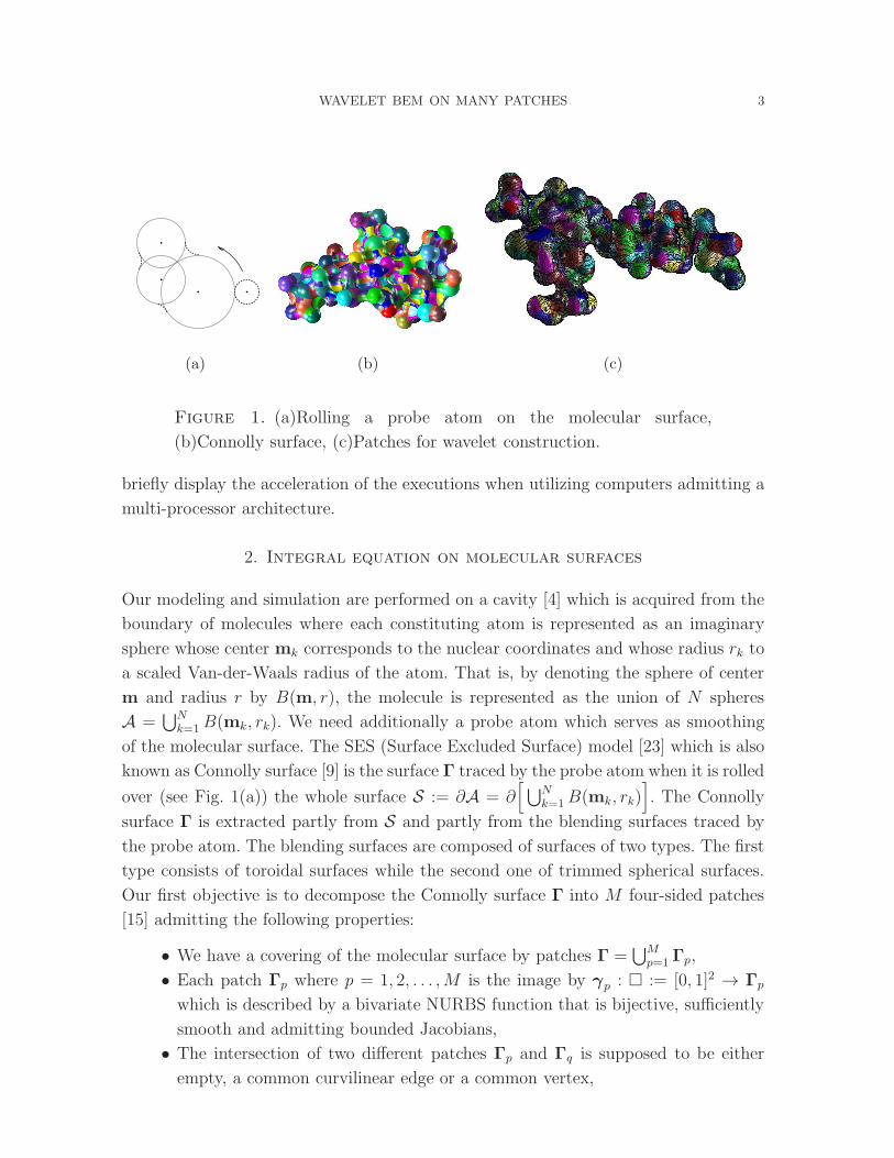
Figure 1. (a)Rolling a probe atom on the molecular surface,

(b)Connolly surface, (c)Patches for wavelet construction.

briefly display the acceleration of the executions when utilizing computers admitting a

multi-processor architecture.

2. Integral equation on molecular surfaces

Our modeling and simulation are performed on a cavity [4] which is acquired from the

boundary of molecules where each constituting atom is represented as an imaginary

sphere whose center mk corresponds to the nuclear coordinates and whose radius rk to

a scaled Van-der-Waals radius of the atom. That is, by denoting the sphere of center

m and radius r by B(m, r), the molecule is represented as the union of N spheres

A =⋃N

k=1B(mk, rk). We need additionally a probe atom which serves as smoothing

of the molecular surface. The SES (Surface Excluded Surface) model [23] which is also

known as Connolly surface [9] is the surface Γ traced by the probe atom when it is rolled

over (see Fig. 1(a)) the whole surface S := ∂A = ∂[⋃N

k=1B(mk, rk)]. The Connolly

surface Γ is extracted partly from S and partly from the blending surfaces traced by

the probe atom. The blending surfaces are composed of surfaces of two types. The first

type consists of toroidal surfaces while the second one of trimmed spherical surfaces.

Our first objective is to decompose the Connolly surface Γ into M four-sided patches

[15] admitting the following properties:

• We have a covering of the molecular surface by patches Γ =⋃M

p=1 Γp,

• Each patch Γp where p = 1, 2, . . . ,M is the image by γp : := [0, 1]2 → Γp

which is described by a bivariate NURBS function that is bijective, sufficiently

smooth and admitting bounded Jacobians,

• The intersection of two different patches Γp and Γq is supposed to be either

empty, a common curvilinear edge or a common vertex,


• The patch decomposition has a global continuity: for each pair of patches Γp,

Γq sharing a curvilinear edge, the parametric representation is subject to a

matching condition. That is, a bijective affine mapping Ξ : → exists

such that for all x = γp(s) on the common curvilinear edge, one has γp(s) =

(γqΞ)(s). In other words, the images of the NURBS functions γp and γq agree

pointwise at common edges after some reorientation,

• The manifold Γ is orientable and the normal vector n(x) is consistently pointing

outward for any x ∈ Γ.

For each patch Γp, the Gram determinant is denoted

(2.1) Gp(t) = Gp(t1, t2) :=

∥∥∥∥∂γp

∂t1(t)×

∂γp

∂t2(t)

∥∥∥∥ ∀ t = (t1, t2) ∈ .

The space of square integrable functions is

(2.2) L2(Γ) :=

f : Γ → R,

∫

Γ

∣∣f(x)∣∣2dΓx <∞

which is equipped with the following scalar product and norm after transformation

onto ,

〈u, v〉L2(Γ) :=

∫

Γ

u(x)v(x)dΓx =M∑

p=1

∫

u(γp(t)

)v(γp(t)

)Gp(t)dt,(2.3)

∥∥v∥∥L2(Γ)

:=[〈v, v〉L2(Γ)

]1/2.(2.4)

The Sobolev space on Γ for a non-negative integer k is

(2.5) Hk(Γ) :=

f ∈ L

2(Γ) :∥∥∂αf

∥∥L2(Γ)

<∞ for all |α| ≤ k

where the differentiation ∂αf is interpreted in the sense of distribution [37] such that

〈∂αf, g〉L2(Γ) = (−1)|α|〈f, ∂αg〉L2(Γ) for all compactly supported smooth functions g.

The Sobolev space Hk(Γ) is endowed with the norm

(2.6)∥∥f

∥∥2

Hk(Γ):=

∑

|α|≤k

∥∥∂αf∥∥2

L2(Γ).

Concerning a real positive order p = k + θ such that k is an integer and θ ∈]0, 1[, the

Sobolev space Hp(Γ) consists of the functions such that their norms with respect to

the next Slobodeckij norm are finite

(2.7)∥∥f

∥∥2

Hp(Γ)=

∥∥f∥∥2

Hk(Γ)+

∑

|α|=k

∫

Γ×Γ

|∂αf(x)− ∂αf(y)|2

‖x− y‖2+2θdΓx dΓy.

For negative orders, one employs the dual spaces H−p(Γ) =[Hp(Γ)

]∗. By designating

the region enclosed within Γ by Ω ⊂ R3, our second objective is to solve the interior


problem:

(2.8)

∆U(x) = 0 for x ∈ Ω

U(x) = g(x) for x ∈ Γ = ∂Ω = ∪Mp=1Γp.

Introduce the double layer operator

(K v)(x) =1

4π

∫

Γ

∂

∂n(y)

[1

‖x− y‖

]u(y)dΓy(2.9)

=1

4π

∫

Γ

〈n(y),x− y〉

‖x− y‖3u(y)dΓy.(2.10)

In the general case, we have the following mapping using Sobolev spaces

(2.11) K : H1/2(Γ) −→ H1/2(Γ)

which is linear and continuous. In the current case, since the entire molecular surface

Γ is sufficiently smooth, we have

(2.12) K : H(1/2)+s(Γ) −→ H(1/2)+s(Γ)

for any real number s according to Theorem 7.1 and Theorem 7.2 of [26]. In particular,

we deduce the bounded linearity with respect to square-integrable functions:

(2.13) K : L2(Γ) ≡ H0(Γ) −→ L

2(Γ) ≡ H0(Γ).

We make now the change of unknown

(2.14) U(x) =1

4π

∫

Γ

∂

∂n(y)

[1

‖x− y‖

]u(y)dΓy

by using u as the new unknown which is also termed as density function. As a point

x ∈ Ω approaches x0 ∈ Γ = ∂Ω, we have [26, 3, 18]

(2.15) limx→x0x∈Ω

(Ku)(x) = −1

2u(x0) + (Ku)(x0)

because the manifold Γ contains neither a nonsmooth edge nor a sharp corner. The

function U as mentioned in (2.14) is harmonic in the sense that ∆U = 0. Therefore, in

the case that u satisfies

(2.16) −1

2u(x0) + (Ku)(x0) = g(x0) for x0 ∈ Γ,

then on account of (2.15), the function U = Ku solves the boundary value problem in

(2.8). In operator form, we have the next integral equation after multiplication by (-2):

(2.17) (I− 2K)u = f where f := −2g.

By discretizing (2.17) in some finite dimensional space Vh, one searches for uh ∈ Vh

such that for all vh ∈ Vh

(2.18)

∫

Γ

uh(x)vh(x)dΓx+

∫

Γ

∫

Γ

K(x,y)uh(x)vh(x)dΓxdΓy =

∫

Γ

f(x)vh(x)dΓx


where we use the kernel

(2.19) K(x,y) :=1

2π

〈n(y),y− x〉

‖x− y‖3.

Once the solution u to the integral equation (2.17) becomes available, the solution

U to the initial problem is obtain by (2.14). Since both the wavelet basis function

and the mappings γp are expressed in term of B-spline basis, we shall recall briefly

some important properties of a B-spline setting which represents piecewise polynomials.

Consider two integers n, k such that n ≥ k ≥ 1. Should the interval [a, b] be the domain

of definition of the B-spline, that interval is subdivided by a knot sequence ζ = (ζi)n+ki=0

such that ζi < ζi+1 for i = k− 1, ..., n− 1 and such that the initial and the final entries

of the knot sequence are clamped ζ0 = · · · = ζk−1 = a and ζn = · · · = ζn+k = b. One

defines the B-splines [10, 7, 28] basis functions as

Nζ,ki (t) := (ζi+k − ζi)[ζi, ..., ζi+k](· − t)k−1

+ for i = 0, ..., n

where one employs the divided difference [ζi, ζi+1, ..., ζp]f in which one uses the trun-

cated power functions (· − t)k+ given by (x − t)k+ := (x − t)k if x ≥ t, while it is zero

otherwise. The integer k controls the polynomial degree k − 1 of the B-spline which

admits an overall smoothness of Ck−2 where the case k = 1 corresponds to discontinu-

ous piecewise constant functions needed for the Haar wavelet. The integer n controls

the number of B-spline functions for which each B-spline basis Nζ,ki is supported by

[ζi, ζi+k]. The NURBS patch γp admitting the control points di,j ∈ R3 and weights

wi,j ∈ R+ is expressed as

(2.20) γp(u, v) =

∑ni=0

∑nj=0wi,jdi,jN

ζ,ki (u)Nζ,k

j (v)∑n

i=0

∑mj=0wi,jN

ζ,ki (u)Nζ,k

j (v)∈ R

3 ∀ (u, v) ∈ .

As for the construction of the finite dimensional space Vh, since the Gram determinant

Gp is bounded

(2.21) 0 < c ≤ minp=1,...,M

inft∈

Gp(t) < maxp=1,...,M

supt∈

Gp(t) ≤ C <∞,

the above structure of the surface Γ allows to construct bases on 2D which are carried

over the manifold Γ that is embedded in R3. The Galerkin variational formulation with

respect to a finite dimensional space spanned by (ϕα)mα=1 uses the approximating func-

tions uh(x) =∑m

α=1 uαϕα(x) where UT := [u1, ..., um] ∈ Rm are the BEM-unknowns.

The next linear system is eventually obtained

(2.22) (I+K)U = S


such that the matrix entries and the right hand side are

I(α,β) :=

∫

Γ

ϕα(x)ϕβ(x)dΓx =M∑

p=1

∫

Γp

ϕα(x)ϕβ(x) dΓpx(2.23)

K(α,β) :=

M∑

p=1

M∑

q=1

∫

Γp

∫

Γq

K(x,y)ϕα(x)ϕβ(y)dΓpx dΓq

y(2.24)

Sα :=M∑

p=1

∫

Γp

f(x)ϕα(x)dΓpx.(2.25)

In general, the linear system (2.22) is troublesome because the basis functions (ϕα)mα=1

yield a dense matrix for the operator K. In term of memory, if (ϕα)mα=1 are standard

polynomial basis functions, the matrix K requires m2 storage to accommodate all

entries. In addition, the determination of a matrix entry of K calculates an integration

in 4D where the integrand is highly nonlinear and possibly singular depending on the

patch pair Γp×Γq. By using tensor product B-spline wavelet basis functions, the matrix

K becomes quasi-sparse. For the instance of high-order odd wavelets [24, 25], we depict

on Fig. 2(a) the quasi-sparse matrix entries for a 2D singular operator where very small

entries are set to zero.

3. Patch generation for wavelet bases

Let us specify the assumptions concerning the positions of the nuclei mi and the prop-

erties of the radii ri with respect to the probe radius ρ. For every two arbitrary atoms

B(mi, ri) and B(mj , rj), we assume that one of the following two conditions holds.

(C1) Either the two enlarged spheres B(mi, ri + ρ) and B(mj , rj + ρ) by the probe

radius ρ are completely disjoint such as ‖mi −mj‖ > ri + rj + 2ρ,

(C2) or we have Dij := ‖mi −mj‖ ≤ ri + rj + 2ρ and additionally

2Dijr2i + 4Dijρ−D2

ij − (ri + ρ)2 + (rj + ρ)2 > 0.

Those two assumptions exclude the situation where the blending torus which is tan-

gent to both B(mi, ri) and B(mj , rj) admits a self-intersection. If assumptions (C1)

and (C2) are not fulfilled but one still wants to treat the molecule, one carefully inserts

additional dummy atoms between every two atoms B(mi, ri) and B(mj , rj) for which

there is a toroidal self-intersection. The sizes and the positions of the dummy atoms

should be minimized while keeping the shape of the initial molecule. We will consider

the generation of the constituents of the B-Rep (boundary representation) of the SES

surfaces. For two spheres B1 := B(m1, r1) and B2 := B(m2, r2), we define their power

distance as D(B1,B2) := ‖m1 −m2‖2 − r21 − r22. The i-th Laguerre cell is composed of


(a)

2 2.5 3 3.5 4 4.5 5 5.5 6

−0.04

−0.03

−0.02

−0.01

0

0.01

0.02

0.03

0.04

(b) (c)

Figure 2. (a)Quasi-sparse matrix, (b)Higher-order wavelet on a

nonuniform knot sequence, (c)Bivariate tensor product basis.

points which are closer to Bi than to any other Bj (j 6= i) with respect to the power

distance: Ci :=x ∈ R3 : D

(B(x, 0),Bi

)≤ D

(B(x, 0),Bj

)∀ j 6= i

. A Laguerre

decomposition of R3 with respect to the spheres Bi is R3 =⋃N

i=1Ci. If all radii are

equal, the Laguerre decomposition coincides with the usual Voronoi decomposition as

illustrated in Fig.3(b). For two spheres Bi and Bj , the radical axis is the set of points

which are equidistant to Bi and Bj with respect to the power distance. Such a set is

a plane given by R(Bi,Bj) =x ∈ R3 : 2〈x,mi −mj〉 = ‖mi‖2 − ‖mj‖2 + r2j − r2i

.

The Laguerre cell is a convex polyhedron which has faces from the radical axes and

which could be bounded or unbounded. To obtain the Laguerre decomposition, we

consider the uplifting function which associates to mi = (xi, yi, zi) ∈ R3 the value

mi :=(xi, yi, zi, x

2i + y2i + z2i + r2i

)∈ R4. After generating the convex hull H of the set

of four dimensional points mi, the projection of the lower face of H on the space R3

generates a weighted Delaunay tetrahedral decomposition [12] having apices mi. Each

apex of the Laguerre cell is the orthocenter of a tetrahedron of the weighted Delau-

nay. The Laguerre decomposition is obtained by the dual of the weighted Delaunay.

We describe next the way of obtaining the spherical trimmed surfaces of each atom

Bm by considering its cell Cm. For each neighboring cell Cj of Cm, consider the cell

planar face Pmj which separates the spheres B(mm, rm) and B(mj , rj). One generates

two offset planes pm and pj by orthogonally shifting Pmj by dm := Dmjρ/(rm + ρ)

and dj := Dmjρ/(rj + ρ) toward those two spheres respectively. Two circles cm and cj

are traced on those spheres by pm and pj . We discard the circular arcs on Bm which

are either included inside an atom other than Bm or between the planes pm, pj . By

organizing the remaining circular arcs, we obtain several closed curves on the sphere

Bm. These bounding curves yield several spherical trimmed surfaces on the sphere Bm.

Each face Pmj of the Laguerre decomposition corresponds to one torus Tmj which is


tangent upon Bm and Bj . To obtain the toroidal surface, we trim off the toroidal part

of Tmj which is beyond the parallel planes pm, pj. If the rolling probe atom touches at

least three atoms, we construct a spherical blend whose boundary is composed of the

arcs which are the intersections of the toroidal surface Tmj and the probe atom. At this

point, we have subsurfaces Si which are bounded by some circular arcs. Stereographic

projections serve as parametrizations of the subsurfaces Si from some trimmed planar

domains. We describe now the decomposition of a Connolly surface into large four-sided

subsurfaces. We use a triangular mesh M of the whole surface as an intermediate step.

We determine first the underlying structure of a coarse quadrangulation Qcoarse. We

deduce the nodes, edges and quadrilaterals of Qcoarse from the mesh. We start from a

fine quadrangulation Qfine which is obtained by subdividing each triangular element of

M into three quadrilaterals. The resulting quadrangulation Qfine is not directly useful

for patch representation because it is too fine. As a consequence, we need to coarsen

that fine quadrangulation repeatedly in which we initialize Q0 := Qfine. Each coarsen-

ing step from Qm to Qm+1 consists in amalgamating a few neighboring quadrilaterals

in the quadrangulation Qm to form a coarser local simplified quadrangulation in Qm+1.

It is a long programming to implement many local patterns of simplification and to

recursively determine the parts of Qm to coarsen so that the final patches have simi-

lar surface areas. Since the initial finest quadrangulation Qfine is inappropriate to be

used as Qcoarse, we impose minimal and maximal numbers of coarse quadrilaterals. For

the recursive quadrangulation simplification, we use a coarsening parameter α ∈ [0, 1]

which gauges the density of Qcoarse. A unit value of α corresponds to the finest allowed

quadrilateral decomposition while a value of α approaching zero corresponds to a very

coarse quadrilateral decomposition. After assembling Qcoarse having straight edges, we

need to connect every two nodes Pi and Pj on the endpoints of every edge by a curve on

the manifold as illustrated in Fig. 3(a). That curve is described by means of a geodesic

curve on M joining Pi to Pj. First, we need a curve which traverses only the nodes

and the edges of M. Afterward, we improve that curve by allowing it to traverse the

internal parts of the triangles of M. Assembling the complete node-edge graph of the

whole mesh M is very memory consuming. Searching for shortest paths becomes very

cumbersome for such a large discrete manifold. Some efficient data structure to accel-

erate the search is necessary in the implementation. We eventually fit each four-sided

submeshes by NURBS patches where each interface curve has a matching parametriza-

tion by its incident patches. During the application of those geometric operations, tests

must be performed in order to avoid manifold folding and tiny gaps. Many tests related

to edge degeneration and angular quality are needed to be applied in practice.

In order to ensure the validity of conditions (C1) and (C2), one adopts the method

of GEPOL in which some additional spheres are inserted [38, 20]. Those incorporated


(a)

0 0.1 0.2 0.3 0.4 0.5 0.6 0.7 0.8 0.9

0.1

0.2

0.3

0.4

0.5

0.6

0.7

0.8

0.9

(b)

Figure 3. (a)Curvilinear edges traced on the manifold, (b)Centered

convex decomposition of the space.

extra-spheres are not physically relevant. These are fictive spheres admitting neither

atomic masses nor electric charges. The principal objective of the previously mentioned

conditions is to avoid the conflicting situation where some toroidal blending surfaces

occur when the corresponding two disjoint atoms are distant from one another so that

the contact with the probe atom is almost tangential. In such a case, a self-intersecting

toroidal blend is formed. In order to remedy that problem, a fictive non-atom centered

sphere is inserted between every two atoms where those conditions are violated. It is

worth noting anyhow that such a situation occurs only in very rare cases. We would like

to explain the similarity and the difference between the above two types of smoothing

surfaces which are the toroidal ones and the spherical ones. Both surfaces serve as

blending surfaces between neighboring atoms. The principal difference between them

is that the toroidal ones occur when only two atoms are touched by the probe atom,

whereas a spherical blend appears when more than two atoms simultaneously have

contact with the probe atom as illustrated in Figure 1(a) and Figure 1(b). In the latter

case, the number of atoms which touch the probe atom is three in most practical cases

but that number can theoretically be arbitrarily many depending on the positions and

the radii of the constituting atoms.

Now that we have a four-sided decomposition, we want to construct the wavelet spaces

on the surface Γ. Since every two incident patches admit pointwise joints, constructing

the wavelet bases on the unit square is sufficient to construct basis functions on

the whole molecular surface. Each 1D-wavelet basis will be constructed as a linear


combination of B-splines

(3.26) ψ(t) =

n∑

i=0

qiNζ,ki (t) ∈ R where ∀ t ∈ [0, 1].

On level ℓ, we define a knot sequence ζℓ = (ζℓi ) ⊂ [0, 1] such that ζℓi = 0 and ζℓn+1+i = 1

for i = 0, ..., k and that the remaining ζℓi ∈]0, 1[. The internal knots on the next level

(ℓ + 1) are obtained by inserting one new knot inside two consecutive knots on the

lower level ℓ. Introduce the B-spline linear space on level ℓ:

(3.27) Vkℓ [0, 1] :=

N ℓ

i := Nζℓ,ki ∈ L2[0, 1] : i = 0, ..., n

.

By using the piecewise polynomial property of the B-splines and the inclusion ζℓ ⊂

ζℓ+1, the B-spline bases form a nested sequence of subspaces:

(3.28) Vk1[0, 1] ⊂ V

k2[0, 1] ⊂ · · · ⊂ V

kL[0, 1] ⊂ L2[0, 1].

As a consequence, the space Vkℓ [0, 1] can be expressed as an orthogonal sum

(3.29) Vkℓ [0, 1] = V

kℓ−1[0, 1]⊕W

kℓ−1[0, 1]

with respect to the L2-scalar product where Wkℓ [0, 1] is the wavelet space

(3.30) Wkℓ−1[0, 1] = span

ψℓ−1i ∈ V

kℓ [0, 1], 〈ψℓ−1

i , φ〉L2[0,1] = 0, ∀φ ∈ Vkℓ−1[0, 1]

.

By applying the decomposition (3.29) recursively, one obtains on the maximal level L

(3.31) VkL[0, 1] = V

k1[0, 1]⊕

( L−1⊕

ℓ=1

Wkℓ [0, 1]

).

The 2D-wavelet spaces (see Fig.2(c)) on the unit square is defined for any maximal

level L as follows.

(3.32) VkL() := V

kL[0, 1]⊗ V

kL[0, 1] = A

k()⊕ BkL()⊕ C

kL()⊕ D

kL()

such that

Ak() := V

k1[0, 1]⊗ V

k1[0, 1], B

kL() :=

L−1⊕

ℓ=1

(W

kℓ [0, 1]⊗ V

k1[0, 1]

),

CkL() :=

L−1⊕

ℓ=1

(V

k1[0, 1]⊗W

kℓ [0, 1]

), D

kL() :=

L−1⊕

ℓ=1

L−1⊕

m=1

(W

kℓ [0, 1]⊗W

km[0, 1]

).

We want now to survey the determination of the wavelet bases ψℓi of Wk

ℓ [0, 1]. The

construction of the higher-order wavelets [24, 25] requires the case on the whole infinite

real line R on which one has knot entries on each integer as ζi := i. The cardinal B-

spline is given by

(3.33) NCARDINALi (x) =

∫ 1

0

NCARDINALi−1 (x− t)dt


Molecules Nb. atomsNumber of patches (Runtime in second)

α = 0.2 α = 0.3 α = 0.4

Benzene 12 84 (13.86 s) 97 (14.06 s) 119 (14.60 s)

Cyclohexane 18 99 (15.27 s) 108 (16.27 s) 127 (16.13 s)

LDS 49 286 (50.36 s) 346 (53.73 s) 409 (52.76 s)

Streptomycin 81 399 (68.69 s) 468 (67.78 s) 564 (74.02 s)

Lecithin 128 687 (118.50 s) 821 (120.68 s) 932 (145.11 s)

PDMPG 225 1102 (219.23 s) 1345 (219.12 s) 1556 (226.34 s)

DNA 116 1610 (461.67 s) 1899 (475.33 s) 2232 (487.38 s)

Table 1. Number of patches with respect to the number of atoms and

the coarseness factor α.

which verifies the two scale relation

(3.34) NCARDINALi (x) =

i∑

j=0

2−i+1

(j

i

)NCARDINAL

i (2x− j).

For the polynomial degree k, the corresponding complementary space is spanned by

the shifts of the wavelet function

(3.35) ψCARDINAL(x) :=1

2k−1

2m−2∑

j=0

(−1)jNCARDINAL2k (j + 1)

dk

dxkNCARDINAL

2k (2x− j).

Representing the derivatives dkNCARDINAL2k (2x− j)/dxk in function of B-splines can be

used to express the function ψCARDINAL in term of control points. The cardinal wavelets

are orthogonal to B-splines on the infinite real line R having integers as knot sequence.

The cardinal splines serve as construction of internal wavelets on the interval [0, 1] by

scaling and shifting. Only the odd wavelets for odd polynomial degree k is described

because the even case is defined almost similarly with the exception of additional central

wavelets. One defines on level ℓ the clamped knot sequence ζℓ0 = · · · = ζℓk−1 = 0, and

ζℓnℓ= · · · = ζℓnℓ+k = 1 where nℓ := 2ℓ−1. The dependence on ℓ is sometimes dropped to

simplify the notations. The 1D-wavelets use the following internal knot sequence ζ(ℓ)

(3.36) ζℓj :=(⌊k/2

⌋+ j

)2−ℓ ∈]0, 1[, for j = k, ..., nℓ

The internal wavelet functions are defined by means of scaled and dilated transforma-

tions

(3.37) ψℓj(t) := ψCARDINAL

(2ℓt− (j − k + 1)

).


Additionally, one needs boundary wavelet functions which are of the form

(3.38) ψℓj(t) =

k+⌊k2⌋−2∑

p=0

qp,ℓNℓ+1p (t) +

k+⌊k2⌋+2ℓ∑

p=k+⌊k2⌋−1

qp,ℓNℓ+1p (t)

where the coefficients qp,ℓ for the last summation are the control points of the car-

dinal wavelet ψCARDINAL. the control points of the cardinal wavelet ψCARDINAL. The

remaining unknown coefficients qp,ℓ on the first summation are obtained by solving

(3.39)

k+⌊k2⌋−2∑

p=0

⟨N ℓ+1

p , N ℓm

⟩L2[0,1]

qp,ℓ = −

k+⌊k2⌋+2ℓ∑

p=k+⌊k2⌋−1

qp,ℓ⟨N ℓ+1

p (t), N ℓm

⟩L2[0,1]

,

for m = 0, ..., k + ⌊k2⌋ − 2. That ensures the L2-orthogonality

(3.40) 〈ψℓj , N

ℓm〉L2[0,1] = 0, ∀N ℓ

m ∈ Vkℓ [0, 1].

The previous construction creates 2ℓ−1 wavelet basis functions. To complete the con-

struction, the remaining ones are deduced by symmetry such as ψℓj(t) := ψℓ

2ℓ−j−1(1− t)

for t ∈ [0, 1], j = 2ℓ−1, ..., 2ℓ − 1. The construction of the Haar wavelets and piecewise

linear wavelets is very similar. The former corresponds to piecewise constant polyno-

mials while the latter to piecewise polynomials of degree unity. Since every polynomial

of degree (k − 1) can be expressed in term of N ℓi , we obtain from the orthogonality

(3.40) the property of vanishing moments:

(3.41)

∫ 1

0

(t− t)pψℓj(t)dt = 0, for 0 ≤ p ≤ k − 1

for any fixed t. It is an important property because it yields quasi-sparse structure of

the matrix K. By using the constructed wavelet basis, we are interested in the values

K(α,β) =

M∑

p=1

M∑

q=1

∫

×

Kp,q(u,v)ψα(u)ψβ(v)du dv,(3.42)

Kp,q(u,v) := K(γp(u),γq(v)

)Gp(u)Gq(v).(3.43)

We will drop the indices of Kp,q since we consider the integrals in the above summation

for a fixed pair Γp × Γq. By fixing some (u, v) = [(u1, u2), (v1, v2)] ∈ × and by

considering any (u,v) = [(u1, u2), (v1, v2)] ∈ ×, the Taylor expansion yields

K(u,v) =∑

|α|+|β|≤k−1

1

α!

1

β!

∂|α|

∂uα

∂|β|

∂vβK(u, v)(u− u)α(v − v)β +(3.44)

∑

|α|+|β|=k

Rp,qα,β(u,v)(u− u)α(v − v)β.(3.45)


For the first summation, by multiplication with a tensor product wavelet basis ψp ⊗

ψq=(ψp1 ⊗ ψp

2) ⊗(ψq1 ⊗ ψq

2) and by taking the integration over × , one obtains for

α = (α1, α2) and β = (β1, β2) where |α| = |α1|+|α2| ≤ k−1 and |β| = |β1|+|β2| ≤ k−1

(3.46)1

α!

1

β!

∂|α|

∂uα

∂|β|

∂vβK(u, v)

∫ 1

0

(u1 − u1)α1ψp

1(u1)du1 · · ·

∫ 1

0

(v2 − v2)β2ψq

2(v2)dv2

which is zero due to the property of the vanishing moment (3.41). As for the sec-

ond summation, introduce ηr := maxi=1,2

|ui − ui| where (u1, u2) ∈ Support(ψr)

for r = p, q. The summation is estimated by∑

|α|+|β|=k

∣∣Rα,β(u,v)∣∣ maxu∈

∣∣ψp(u)∣∣

maxv∈∣∣ψq(v)

∣∣ η|α|p η

|β|q . By defining η := maxηp, ηq < 1, one obtains

(3.47) ηk∑

|α|+|β|=k

max(u,v)∈×

∣∣Rp,qα,β(u,v)

∣∣ maxu∈

∣∣ψp(u)∣∣ max

v∈

∣∣ψq(v)∣∣

Due to boundedness (2.21), one obtains for x = γp(u) ∈ γp

[Support(ψp)

]and y =

γq(v) ∈ γq

[Support(ψq)

]on account of the Calderon-Zygmund inequality in the case

|α|+ |β| = k:

(3.48)∣∣Rp,q

α,β(u,v)∣∣ ≤ C

∣∣∣∂|α|

∂xα

∂|β|

∂yβK(x,y)

∣∣∣ ≤ C1

‖x− y‖k+1

which is small if the images γp

[Support(ψp)

]and γq

[Support(ψq)

]are sufficiently

distant from one another. Thus, the speed of the decay toward zero depends on the

factor ηk using the vanishing moments exponent k and the distances between the basis

supports. Hence, the constructed wavelet basis has the advantage that it renders the

operator K quasi-sparse.

4. Wavelet hierarchy and integration

This section is occupied by the efficient computation of the matrix entries from (3.42).

Since our method is based on a hierarchical tree on the B-spline knots, we describe

next the procedure of inserting new knots into existing ones. The principal objective

is to be able to efficiently express a function defined on the coarse knot sequence in

term of B-splines on a fine one. Consider two knot sequences ζℓ = (ζℓ0, ..., ζℓnℓ+k) and

ζℓ+1 = (ζℓ+10 , ..., ζℓ+1

nℓ+1+k) such that ζℓ ⊂ ζℓ+1. For both knot sequences, the smoothness

index k is conserved intact. One introduces

φki (y) := (y − ai)

0+Ψ

ki (y), for some ai ∈ [ζℓ+1

j , ζℓ+1j+k)

(y − ai)0+ := 1 if y > ai,

(y − ai)0+ := 0 if y ≤ ai,

where Ψki (t) := (t− ζℓ+1

i+1 ) · · · (t− ζℓ+1i+k−1). The discrete B-splines are defined as

(4.49) αki (r) := (ζℓi+k − ζℓi )[ζ

ℓi , · · · , ζ

ℓi+k]φ

kr


Figure 4. Patch representation of a DNA section with 1905 NURBS.

which enables to express the basis in lower level in term of those in higher level such

as

Nζℓ,ki (x) =

m∑

r=0

αki (r)N

ζℓ+1,kr (x).

The De-Boor algorithm for the evaluation of the discrete B-splines αki (p) utilizes the

recurrence

α1i (j) = 1 if ζℓ+1

j ∈ [ζℓi , ζℓi+j)

α1i (j) = 0 if ζℓ+1

j 6∈ [ζℓi , ζℓi+j)

αki (j) = (ζℓ+1

j+k−1 − ζℓi )βk−1i (j) + (ζℓi+k − ζℓ+1

j+k−1)βk−1i+1 (j)

in which βki (j) := αk

i (j)/(ζℓi+k − ζℓi ) for ζℓi+k > ζℓi while βk

i (j) = 0 otherwise. We will

write interchangeably ζℓi ≡ ζℓ[i]. In addition, for a knot entry ζℓi on level ℓ, we denote

by p(i) the index on level ℓ+ 1 such that

(4.50) ζℓ[i] = ζℓ+1[p(i)].

Since one inserts one (ℓ + 1)-knot entry between two consecutive ℓ-knot entries, one

has in particular

(4.51) ζℓ[i+ 1] = ζℓ+1[p(i) + 2], thus p(i+ 1) = p(i) + 2.


We introduce the the following 4D-voxels

(4.52) [ℓ1,ℓ2,ℓ3,ℓ4][i1,i2,i3,i4]

:= [ζℓ1i1 , ζℓ1i1+1]× [ζℓ2i2 , ζ

ℓ2i2+1]× [ζℓ3i3 , ζ

ℓ3i3+1]× [ζℓ4i4 , ζ

ℓ4i4+1].

We will use the next multi-indices for the wavelet and B-spline bases

(4.53) ψ[ℓ1,ℓ2,ℓ3,ℓ4][i1,i2,i3,i4]

:= ψℓ1i1⊗ ψℓ2

i2⊗ ψℓ3

i3⊗ ψℓ4

i4, N

[ℓ1,ℓ2,ℓ3,ℓ4][i1,i2,i3,i4]

:= N ℓ1i1⊗N ℓ2

i2⊗N ℓ3

i3⊗N ℓ4

i4.

Since the tensor product wavelet bases verify

(4.54) ψ[ℓ1,ℓ2,ℓ3,ℓ4][i1,i2,i3,i4]

=∑

(j1,j2,j3,j4)

q(j1,j2,j3,j4)N[ℓ1,ℓ2,ℓ3,ℓ4][j1,j2,j3,j4]

,

it suffices to compute ∫

[ℓ1,ℓ2,ℓ3,ℓ4]

[i1,i2,i3,i4]

K(t)N[ℓ1,ℓ2,ℓ3,ℓ4][j1,j2,j3,j4]

(t) dt.

For the Haar wavelets where the corresponding B-spline are piecewise constant, we

have four recurrences:∫

[ℓ1,ℓ2,ℓ3,ℓ4]

[i1,i2,i3,i4]

K(t) dt =

∫

[ℓ1+1,ℓ2,ℓ3,ℓ4]

[p(i1),i2,i3,i4]

K(t) dt+

∫

[ℓ1+1,ℓ2,ℓ3,ℓ4]

[p(i1)+1,i2,i3,i4]

K(t) dt.(4.55)

= · · ·(4.56)

=

∫

[ℓ1,ℓ2,ℓ3,ℓ4+1]

[i1,i2,i3,p(i4)]

K(t) dt+

∫

[ℓ1,ℓ2,ℓ3,ℓ4+1]

[i1+1,i2,i3,p(i4)+1]

K(t) dt.(4.57)

For wavelets admitting higher polynomial degrees, by using the discrete B-splines one

also obtains four recurrences including:∫

[ℓ1,ℓ2,ℓ3,ℓ4]

[i1,i2,i3,i4]

K(t)N[ℓ1,ℓ2,ℓ3,ℓ4][j1,j2,j3,j4]

(t) dt =m∑

r=0

αkj1(r)

∫

[ℓ1+1,ℓ2,ℓ3,ℓ4]

[p(i1),i2,i3,i4]

K(t)N[ℓ1+1,ℓ2,ℓ3,ℓ4][r,j2,j3,j4]

(t) dt+

+

∫

[ℓ1+1,ℓ2,ℓ3,ℓ4]

[p(i1)+1,i2,i3,i4]

K(t)N[ℓ1+1,ℓ2,ℓ3,ℓ4][r,j2,j3,j4]

(t) dt.

Our objective is to avoid computing any involved integrals several times. Therefore, we

construct a hierarchical tree whose nodes correspond to the 4D-voxels [ℓ1,ℓ2,ℓ3,ℓ4][i1,i2,i3,i4]

. We

define the depth of the multilevel ℓ = (ℓ1, ℓ2, ℓ3, ℓ4) having 4D-indices to be ∆(ℓ) = ℓ1+

ℓ2+ℓ3+ℓ4. Each tree-node has offsprings [ℓ1+1,ℓ2,ℓ3,ℓ4][p(i1),i2,i3,i4]

, [ℓ1+1,ℓ2,ℓ3,ℓ4][p(i1)+1,i2,i3,i4]

,..., [ℓ1,ℓ2,ℓ3,ℓ4+1][i1,i2,i3,p(i4)]

,

[ℓ1,ℓ2,ℓ3,ℓ4+1][i1,i2,i3,p(i4)+1]. By using the above recurrences, one traverses the hierarchical tree

bottom-up in order to obtain the integrals on all relevant 4D-voxels [ℓ1,ℓ2,ℓ3,ℓ4][i1,i2,i3,i4]

. Thus,

the wavelet integrals are computed hierarchically without doing any repeated compu-

tations. That is, one starts from the voxels having the largest depth ∆max(ℓ). The worst

case of the depth of the hierarchical tree is 4L depending on the wavelet indices chosen

in the quasi-sparse structure. For the current paper, we use the Genz-Malik integration

[13] to compute the integrals corresponding to the leaves of the hierarchical tree. In a


forthcoming paper, we will present a more efficient method for computing the leaf in-

tegrals. The integration on the voxels [ℓ1,ℓ2,ℓ3,ℓ4][i1,i2,i3,i4]

are computed by transforming it onto

[−1, 1]4. The Genz-Malik method evaluates the integral∫ 1

−1

∫ 1

−1· · ·

∫ 1

−1F (x1, x2, ..., xD)

dx1 dx2 ... dxD of a multivariate function F : [−1, 1]D −→ R by utilizing the 7-point

rule

SP [F ] = w1F (0, ..., 0) + w2

∑

p=±1

D∑

i=1

(IiF )(pλ2) + w3

∑

p=±1

D∑

i=1

(IiF )(pλ3) +

w4

∑

p=±1

D∑

i<j

(Ji,jF )(pλ4) + w4

∑

p=±1

F (pλ5, ..., pλ5),

(IiF )(pλ) := F (0, ..., 0, pλ, 0, ..., 0),

(Ji,jF )(pλ) := F (0, ..., 0, pλ, 0, ..., 0, pλ, 0, ..., 0).

The nonzero entry (resp. entries) of IiF is (resp. JijF ) at the i-th position (resp. i-th

and j-th positions). In the 4D cases, every application of SP [F ] requires 57 function

evaluations. For the determination of the parameters in SP , one solves a nonlinear

system [13] involving the functions

N1(w1, ..., w5) = w1 + 2Dw2 + 2Dw3 + 2D(D − 1)w4 + 2Dw5

N2(w1, ..., w5) = 2λ22w2 + 2λ23w3 + 4(D − 1)λ24w4 + 2Dλ25w5

...

N7(w1, ..., w5) = 2Dλ65w5 + 2D/27.

The solution to that nonlinear system gives exactly λ22 = 9/70, λ23 = λ24 = 9/10,

λ25 = 9/19 while the weights are w1 = 2D(12824 − 9120D + 400D2)/19683, w2 =

2D(980/6561), w3 = 2D(1820−400D)/19683, w4 = 2D(200−19683), w5 = 6859/19683.

That integrator is combined with some adaptive subdivision in which D-dimensional

hypercubes that produce large integration errors are split into smaller ones. That sub-

division starts from [−1, 1]D as the initial hypercube. During the recursive subdivision,

the hypercubes to be split have to be identified. In order to evaluate the local error

inside a hypercube, an error estimator is achieved by the next 5-point rule

FP[F ] = v1F (0, ..., 0) + v2∑

p=±1

D∑

i=1

(IiF )(pλ2) + v3∑

p=±1

D∑

i=1

(IiF )(pλ3) +

v4∑

p=±1

D∑

i<j

(Ji,jF )(pλ4)

where the weights are v1 = 2D(729 − 950D + 50D2)/729, v2 = 2D(245/486), v3 =

2D(265−100D)/1458, v4 = 2D(25/729). In order not to evaluate the integrand too many


Molecules Number of patches area/(neighb area) Global ratio

Benzene 12 0.960095 0.706800

Cyclohexane 97 0.959639 0.695809

Tamoxifen 410 1.012924 0.665099

Streptomycin 462 0.959130 0.662762

Lecithin 821 0.971143 0.676250

PDMPG 2175 1.015307 0.688102

DNA 3144 0.950066 0.651584

Table 2. Investigation of patches area.

times, the integration points for FP are taken from the 7-point rule SP . The error

estimator is the difference between SP and FP. As input, one accepts the maximal

number of integrand evaluations together with the desired accuracy. We apply the

above numerical quadrature to K(u,v) in which we avoid zero division by replacing

the kernel involving 1/‖x − y‖ by 1/√

‖x− y‖2 + δ for x ∈ Γp, y ∈ Γq where δ > 0

is an adjustable small parameter. A similar approach using δ > 0 has been used in [1]

for the purpose of quantum mechanics using high-dimensional approximation.

5. Wavelet simulation on molecular models

We want now to present some results of the former method which was implemented in

C functions together with C++ classes. The visualization has been implemented with

the help of OpenGL. The computations have been executed on a computer possessing a

4.1 GHz processor and 32 GB RAM. The C-packet cubature [19] serves as computation

of the Genz-Malik integrations. We employ different sorts of quantum models including

water clusters which are obtained from a former MD (Molecular Dynamics) simulation.

When the MD-iteration attains its equilibrium state where the total energy (sum of the

kinetic energy and the potential energy) becomes stable, a water cluster is obtained by

extracting the water molecules which are contained in some given large sphere whose

radius controls the final size of the water cluster. The hydrogen and oxygen atoms

contained in that large sphere constitute the components of the water clusters. We use

also other molecules which are acquired from PDB files.

We would like to provide some numerical results pertaining to the runtimes of the

cavity generation and the quality of the patches. The runtimes depend on several

factors. First, it is affected by the number of atoms in the molecule. Second, it varies

in relation with the atom distributions. Further, it depends on how coarse the patch

decomposition should be. As a first numerical test, we investigate the number of patches


L-valueMolecules Number of patches

Average Ratio with Lideal

Benzene 133 0.595737 0.758516

Quinine 358 0.554006 0.705383

Borane 812 0.531560 0.676803

Lecithin 821 0.555027 0.706682

Water cluster 1567 0.571700 0.727911

DNA 3348 0.576848 0.734465

Table 3. Quality of the resulting patches.

in accordance to the size of the molecule. The results of such a test are gathered in

Tab. 1 where we examine the coarsening Qcoarse from Section 3. According to our

experience, the interesting practical values of α range between 0.2 and 0.4. A smaller

value of α indicates that one has a coarser decomposition which amounts also to a

fewer number of fitting tasks. On the other hand, a single large NURBS surface area

needs many sampling points which mean also that it takes more time to complete

the NURBS determination. Hence, the running time depends not only on the initial

molecular size but also on the surface area of the cavity. For example, lecithin has

more atoms than DNA but the latter takes almost four times longer than the former.

The purpose of the second test is the investigation of the area µ(Γi) of each patch Γi.

Solution U1(x) Solution U2(x)

Absol. Error Relat. Error Reduc. Absol. Error Relat. Error Reduc.

Water cluster (1109 patches):

Lev 1 2.415E-01 8.322E-03 — 1.186E+00 6.752E-03 —

Lev 2 1.327E-01 4.572E-03 1.820 4.984E-01 2.837E-03 2.211

Lev 3 2.456E-02 8.464E-04 5.404 1.347E-01 7.670E-04 3.698

Lev 4 2.430E-03 8.374E-05 10.10 2.989E-02 1.702E-04 4.506

DNA section (2119 patches):

Lev 1 2.081E+00 1.309E-01 — 3.853E-01 4.216E-03 —

Lev 2 1.218E+00 7.666E-02 1.707 1.942E-01 2.125E-03 1.984

Lev 3 4.025E-01 2.532E-02 3.027 4.003E-02 4.380E-04 4.851

Lev 4 4.829E-02 3.038E-03 8.334 1.230E-02 1.346E-04 3.254

Table 4. Error reductions for water cluster and DNA section.

We would like to compare the areas of the patches in two perspectives: in the vicinity


of each patch and global comparison. For the vicinity test, let Ni denote the set of

neighboring patches which share at least one corner node with a patch Γi. We computed

M(i) := µ(Γi)/[

1mi

∑j∈Ni

µ(Γj)]where mi = Card(Ni). The results for the average

values ofM(i) are collected in the third column of Tab. 2 where we observe that the sizes

of the patches vary slowly because M(i) approximates averagely the unity. As for the

global comparison, the ideal patch area µideal is the area of the whole molecular surface

divided by the number of patches. We compute the ratio R(i) := minµ(Γi)

/µideal,

µideal

/µ(Γi)

∈ [0, 1]. The resulting average values of R(i) are exhibited in the last

column of Tab. 2. We observe that the sizes of the patches are not too different from

the ideal size. In fact, we have in general 0.65µideal ≤ µ(Γi) ≤ 1.34µideal. Those patch

properties enable the subsequent wavelet bases to be proportionally distributed. An

instance of the patch decomposition for the case of a DNA section is depicted on

Fig. 4.

Identity Quasisparse Singularity Linear oper. Total Accuracy


Lev 1 0.28 sc 0.09 sc 15.22 sc 1.44 sc 17.03 sc 1.127E-02

Lev 2 0.32 sc 0.23 sc 27.09 sc 2.20 sc 29.84 sc 1.684E-03

Lev 3 0.45 sc 2.68 sc 32.88 sc 6.39 sc 42.40 sc 4.163E-04

Lev 4 1.34 sc 58.41 sc 8.88 mn 25.93 sc 10.30 mn 9.162E-05

Lev 5 6.84 sc 29.13 mn 144.94 mn 3.29 mn 177.48 mn 3.482E-05


Lev 1 1.28 sc 0.61 sc 44.56 sc 10.22 sc 56.67 sc 8.322e-03

Lev 2 1.35 sc 1.91 sc 92.24 sc 15.16 sc 110.66 sc 4.572e-03

Lev 3 1.68 sc 24.03 sc 3.79 mn 49.16 sc 5.04 mn 8.464e-04

Lev 4 4.17 sc 9.07 mn 71.23 mn 3.84 mn 84.22 mn 8.374e-05

Table 5. Durations of the individual steps for the water clusters.

We focus now on investigating the patch quality which is quantified as follows for a

patch Γm on level L. For each i, j = 0, ..., 2L−1, we consider the quadrilateral Qm(i, j)

having vertices am(i, j) := γm(i/2L, j/2L), am(i + 1, j), am(i + 1, j + 1), am(i, j + 1).

By inserting a diagonal [am(i, j + 1), am(i + 1, j)] in Qm(i, j), one defines two trian-

gles T1 and T2. Two other triangles T3 and T4 are defined by inserting the diagonal

[am(i, j), am(i+ 1, j + 1)]. The quality metric L(Qm(i, j)

):= 0.5

[min

(θ(T1), θ(T2)

)+

min(θ(T3), θ(T4)

)]is used where θ(Tp) is the smallest angle in the triangle Tp.


Figure 5. BEM-Density function on the molecular surface of a DNA section.

0.0001

0.001

0.01

0 1 2 3 4 5

e1e2e3e4e5e6e7

Figure 6. Relative errors for several molecules w.r.t. increasing levels.

The ideal quadrilateral which is a perfect square corresponds to Lideal = 0.25π ≃

0.785398. In Tab. 3, we gather the results of our test which consists in computing the

average values of L over the whole patches. We obtain a satisfactory quality because

the average values of L do not tend to zero. We would like now to describe some

results related to BEM simulation on realistic molecular patches. For the computer

implementation, we use only Haar wavelets but the former method can also be ap-

plied to higher-order wavelets. We examine first the error reductions in term of the

multiscale level for large molecules. The results are collected in Tab. 4 which contains

both the absolute errors and the relative errors. The models consist of a water clus-

ter and a DNA section which admit respectively 1109 patches and 2119 patches. We

consider two exact solutions which are respectively U1(x) = .2x2 − .15y2 − .05z2 and


1

2

3

4

5

6

7

8

1 2 3 4 5 6 7 8

Acc

eler

atio

n of

exe

cutio

n

Number of processors

Propane (75 patches)Water cluster (386 patches)

Water cluster (1109 patches)D.N.A. (2119 patches)

(a)

1

2

3

4

5

6

7

8

1 2 3 4 5 6 7 8

Acc

eler

atio

n of

exe

cutio

n

Number of processors

LEVEL 1LEVEL 2LEVEL 3LEVEL 4

(b)

Figure 7. Acceleration of the computation in term of the number of

processors: (a)Molecules having different patch numbers, (b)Several lev-

els.

U2(x) = exp(.5 x) cos(.5 y) that have vanishing Laplacian. The right hand side g(x) is

the restriction of the function U on the boundary Γ. The error reduction is affected

by the exact solutions but in general the errors reduce satisfactorily in function of the

wavelet levels. The absolute errors are obtained by comparing with the exact solution

at some fixed samples in the interior Ω. A division by the largest value of the exact

solution provides the relative error.

We exhibit in Table 5 the runtimes for the different stages which are required for a

complete BEM simulation. These include: (1)the assembly of the identity operator

I, (2)the determination of the indices which yield quasi-sparse matrix entries, (3)the

computation of the singular integrals in the operator K, (4)the solving of the resulting

linear system. In addition, Table 5 exhibits the required total runtimes for two water

clusters which contain respectively 386 patches and 1109 patches on several multiscale

levels. It turns out that the construction of the identity operator executes very quickly.

The task which mainly dominates the BEM-simulation is the assembly of the singular

operator. Although the determination of the quasi-sparse indices and the solving of

the linear system take some time, they do not last as long as the singular operator. A

GMRes method serves as a solver of the system which is nonsymmetric. Since the time

required for the linear solver is very short compared to the assembly of the matrices, it

is not yet our priority to improve the linear solver. We examine now the general linear

characteristic of the relative errors. In Figure 6, we display the error evolution where

we consider four levels for several molecules and several right hand sides. The curves e1

and e5 correspond to a propane molecule admitting 75 patches. We use a water cluster


admitting 386 patches for e2 and e6 while another water cluster admitting 1109 patches

are used for e3 and e7. The curve e7 corresponds to a DNA section admitting 2119

patches. The exact solution U2 is used for the curves e1 till e4 while the remaining

ones correspond to the solution U1. The error plots lightly vary in function of the

used molecules but in general all the curves exhibit the same slope characteristic. In

fact, they decrease linearly in logarithmic scale in function of the BEM levels. The

implemented BEM simulation is able to treat large molecules. Our program functions

in parallel [36, 41, 42] on computers admitting several cores or multi-processors. The

implementation was accomplished by using a message passing technique which was

practically carried out by means of MPI (Message Passing Interface). The acceleration

of the computation which is also known as speedup is summarized in Figure 7. The

speedup quantifies the ratio between the execution time on a parallel machine having p

processors and the time elapsed on a single processor. The speedup curves indicate that

our implementation scales well by increasing the number of processors implying that the

load of computing tasks is well balanced among the processors and that the cost of inter-

processor communications is not excessive. This consists of the BEM program without

the linear solving which takes no more than 5 percent of the entire BEM computation

(see Table 5) and which functions only sequentially for the time being. All other BEM

stages function on a parallel architecture. The speedup curves concern the execution

time when the number of the processors is increased for two cases: (a) various molecules

possessing different patch counts, (b)increasing wavelet levels. It is beyond the scope of

this paper to provide a full description of the parallel implementation which is deferred

to a subsequent article. An instance of the computed density function defined on the

surface of a DNA section is depicted in Figure 5 where a triangular mesh serves only

as simplification of the graphical presentation.

Conclusion

We constructed a surface structure which is suitable for subsequent BEM-simulation.

The molecular boundary in form of Connolly surface was decomposed into globally

continuous NURBS having similar surface areas. We showed outcomes of BEM simula-

tion on different models possessing many patches. Results pertaining to accuracy and

runtimes have been reported as well. We treated several molecular models which are

acquired from a molecular dynamic simulation or from realistic PDB files.

References

[1] A. AMMAR, F. CHINESTA, Circumventing curse of dimensionality in the solution of

highly multidimensional models encountered in quantum mechanics using meshfree finite

sums decompositions, Lect. Notes in Comput. Sci. Eng. 65, pp. 1–17 (2008).


[2] T. APEL, M. RANDRIANARIVONY, Stability of the discretizations of the Stokes prob-

lem on anisotropic meshes, Math. Comput. Simulat. 61, Nos 3-6, pp. 437–447 (2003).

[3] K. ATKINSON, The numerical solution of integral equations of the second kind. Cam-

bridge University Press (1997).

[4] C. BAJAJ, G. XU, Q. ZHANG, A fast variational method for the construction of adaptive

resolution C2 smooth molecular surfaces, Comput. Methods Appl. Mech. Eng. 198, pp.

1684–1690 (2009).

[5] N. BAKER, D. SEPT, M. HOLST, J. MCCAMMON, The adaptive multilevel finite

element solution of the Poisson-Boltzmann equation on massively parallel computers.

IBM J. Res. Dev. 45, pp. 427–438 (2001).

[6] G. BEYLKIN, On the representation of operators in bases of compactly supported

wavelets, SIAM J. Numer. Anal. 29, No. 6, pp. 1716–1740 (1992).

[7] G. BRUNNETT, Geometric design with trimmed surfaces, Comput. Suppl. 10, pp. 101–

115 (1995).

[8] A. COHEN, I. DAUBECHIES, J. FEAUVEAU, Biorthogonal bases of compactly sup-

ported wavelets. Comm. Pure Appl. Math. 45, No. 5, pp. 485–560 (1992).

[9] M. CONNOLLY, Analytical molecular surface calculation, J. Appl. Cryst. 16, pp. 548–

558 (1983).

[10] C. DE BOOR, G. FIX, Spline approximation by quasi-interpolants. J. Approx. Theory

8, pp. 19–45 (1973).

[11] C. DIEDRICH, D. DIJKSTRA, J. HAMAEKERS, B. HENNIGER, M. RANDRIA-

NARIVONY, A finite element study on the effect of curvature on the reinforcement

of matrices by randomly distributed and curved nanotubes, J. Comput. Theor. Nanosci.

12, No. 9, pp. 2108–2116 (2015).

[12] J. GALLIER, Geometric methods and applications for computer science and engineering,

Springer Verlag, TAM 38 (2000).

[13] A. GENZ, A. MALIK, An adaptive algorithm for numeric integration over an N-

dimensional rectangular region. J. Comput. Appl. Math. 6, No. 4, pp. 295–302 (1980).

[14] H. HARBRECHT, M. RANDRIANARIVONY, From Computer Aided Design to wavelet

BEM, Comput. Vis. Sci. 13, No. 2, pp. 69–82 (2010).

[15] H. HARBRECHT, M. RANDRIANARIVONY, Wavelet BEM on molecular surfaces:

parametrization and implementation, Computing 86, pp. 1–22 (2009).

[16] J. HOSCHEK, D. LASSER, Fundamentals of computer aided geometric design, A.K. Pe-

ters, Wellesley (1993).

[17] G. HSIAO, O. STEINBACH, W. WENDLAND, Domain decomposition methods via

boundary integral equations, J. Comput. Appl. Math. 125, pp. 521–537 (2000).

[18] G. HSIAO, W. WENDLAND, Boundary integral equations, Springer Verlag (2008).

[19] S. JOHNSON, http://ab-initio.mit.edu/wiki/index.php/Cubature, 2010.

[20] A. KLAMT, COSMO-RS: From quantum chemistry to fluid phase thermodynamics and

drug design, Elsevier Science (2005).


[21] B. KLEEMANN, A. RATHSFELD, R. SCHNEIDER, Multiscale methods for boundary

integral equations and their application to boundary value problems in scattering theory

and geodesy. Notes Numer. Fluid Mech. 54, pp. 1–28 (1996).

[22] C. LAGE, C. SCHWAB, Wavelet Galerkin algorithms for boundary integral equations.

SIAM J. Sci. Comput. 20, No. 6, pp. 2195–2222 (1999).

[23] B. LEE, F. RICHARDS, The interpretation of protein structures estimation of stratic

accessibility, J. Mol. Biol. 55, pp. 379–400 (1971).

[24] T. LYCHE, K. MØRKEN, Spline-wavelets of minimal support. In: Numerical Methods

in Approximation Theory, Birkhauser, Basel, pp. 177–194 (1992).

[25] T. LYCHE, K. MØRKEN, E. QUAK, Theory and algorithms for non-uniform spline

wavelets. Multivariate approximation and applications. Cambridge: Cambridge Univer-

sity Press. pp. 152–187 (2001).

[26] W. MCLEAN, Strongly elliptic systems and boundary integral equations. Cambridge Uni-

versity Press, Cambridge (2000).

[27] T. PETERSDORFF, C. SCHWAB, Wavelet approximations for first kind boundary in-

tegral equations on polygons. Numer. Math. 74, pp. 479–519 (1996).

[28] L. PIEGL, W. TILLER, The NURBS book, Springer, Berlin (1995).

[29] M. RANDRIANARIVONY, Anisotropic finite elements for the Stokes problem: a-

posteriori error estimator and adaptive mesh, J. Comput. Appl. Math. 169, No. 2, pp.

255–275 (2004).

[30] M. RANDRIANARIVONY, Domain decomposition for wavelet single layer on geome-

tries with patches, Applied Mathematics 7, No. 15, pp. 1798–1823 (2016).

[31] M. RANDRIANARIVONY, Geometric processing of CAD data and meshes as input

of integral equation solvers, Ph.D. thesis, Technische Universitat Chemnitz, Germany

(2006).

[32] M. RANDRIANARIVONY, On global continuity of Coons mappings in patching CAD

surfaces, Comput.-Aided Design 41, No. 11, pp. 782–791 (2009).

[33] M. RANDRIANARIVONY, On transfinite interpolations with respect to convex domains,

Comput. Aided Geom. Des. 28, No. 2, pp. 135–149 (2011).

[34] M. RANDRIANARIVONY, G. BRUNNETT, Preparation of CAD and molecular sur-

faces for meshfree solvers, Lect. Notes Comput. Sci. Eng. 65, pp. 231–245 (2008).

[35] M. RANDRIANARIVONY, Harmonic variation of edge size in meshing CAD geometries

from IGES format, Lect. Notes Comput. Sci. 5102, pp. 56-65 (2008).

[36] A. RAO, MPI-based parallel Finite Element approaches for implicit dynamic analysis

employing sparse PCG solvers, Adv. Eng. Softw. 36, No. 3, pp. 181–198 (2005).

[37] L. SCHWARZ, Theorie des distribution, Hermann, Paris (1966).

[38] E. SILLA, J. PASCAL-AHUIR, J. TOMASI, R. BONACCORSI Electrostatic interaction

of a solute with a continuum. Improved description of the cavity and of the surface cavity

bound charge distribution. J. Comput. Chem. 8, No. 6, pp. 778–787 (1987).

[39] J. TOMASI, B. MENNUCCI, R. CAMMI, Quantum Mechanical Continuum Solvation

Models, Chem. Rev. 105, pp. 2999–3094 (2005).


[40] V. WEIJO, M. RANDRIANARIVONY, H. HARBRECHT, L. FREDIANI, Wavelet for-

mulation of the Polarizable Continuum Model, J. Comput. Chem. 31, No. 7, pp. 1469–

1477 (2010).

[41] J. ZHANG, A PETSc-based parallel implementation of Finite Element Method for elas-

ticity problems, Math. Probl. Eng. 2, pp. 1–7 (2015).

[42] O. VEGA-GISBERT, J. ROMAN, J. SQUYRES Design and implementation of Java

binding open MPI. Parallel Comput. 59, pp. 1–20 (2016).

Date post:	11-Apr-2019
Category:	Documents
Upload:	doandang
View:	214 times
Download:	0 times

MAHARAVO RANDRIANARIVONY - xdomitri.com · The wavelet bases are constructed on the unit square...

Documents