Road Accident Modelling for Highway Development and Management in Developing Countries: Main Report: Trials in India and Tanzania By J P Fletcher, C J Baguley, B Sexton and S Done Project Report No: PPR095 DFID
Transcript
Road Accident Modelling for Highway Development and Management in Developing Countries:
Main Report: Trials in India and Tanzania
By J P Fletcher, C J Baguley, B Sexton and S Done
Project Report No: PPR095 DFID
i
PROJECT REPORT
Road Accident Modelling for Highway Development and Management in Developing Countries:
Main Report: Trials in India and Tanzania
By J P Fletcher, C J Baguley, B Sexton and S Done
Subsector: Transport
Theme: T1
Project Title: Road Accident Modelling for Highway Development and Management in Developing Countries
Project Reference: R8154
Approvals
Project Manager
Quality Reviewed
Copyright TRL Limited 2006 This document has been prepared as part of a project funded by the UK Department for International Development (DFID) for the benefit of developing countries. The views expressed are not necessarily those of DFID. The Transport Research Laboratory and TRL are trading names of TRL Limited, a member of the Transport Research Foundation Group of Companies.
TRL Limited. Registered in England, Number 3142272. Registered Office: Crowthorne House, Nine Mile Ride, Wokingham, Berkshire, RG41 3GA, United Kingdom.
ii
iii
Road Accident Modelling for Highway Development and Management in developing countries
Final Report: Trials in India and Tanzania
List of Abbreviations ............................................................................................................ 1 Executive Summary.............................................................................................................. 3 1 Introduction ................................................................................................................... 7
1.1 Importance of road accidents .................................................................................. 7 1.2 HDM-4..................................................................................................................... 8 1.3 Safety assessment in road development ................................................................ 8
2 The trial road networks and data collection ............................................................. 10 2.1 Site selection ......................................................................................................... 10 2.2 Data Components ................................................................................................. 17 2.3 Accident data......................................................................................................... 18 2.4 Road environment inventory/survey data.............................................................. 20 2.5 Flow Data .............................................................................................................. 22 2.6 Curvature data....................................................................................................... 23 2.7 Junction survey data ............................................................................................. 24 2.8 Works history data................................................................................................. 24
3 Results: Compilation of data ..................................................................................... 25 3.1 Roads sections, India ............................................................................................ 25 3.2 Roads sections, Tanzania ..................................................................................... 25 3.3 Preliminary simple analyses of raw data ............................................................... 26
4 Results: The Modelling Approaches ......................................................................... 35 4.1 Trial of SafeNET Models ....................................................................................... 35 4.2 Generalised linear modelling trials ........................................................................ 39 4.3 Base rates and factor approach ............................................................................ 49 4.4 Hierarchic approach .............................................................................................. 49
5 Summary and Conclusions........................................................................................ 56 5.1 SafeNet Analysis ................................................................................................... 56 5.2 Hierarchic approach .............................................................................................. 57 5.3 Generalised Linear Modelling................................................................................ 57 5.4 The way forward.................................................................................................... 58
6 Acknowledgements .................................................................................................... 59 7 References................................................................................................................... 59 APPENDIX A Review of Road Accident Modelling..................................................... 62
Appendix A References................................................................................................... 87 APPENDIX B Road Sections Selected for study ........................................................ 92
Tamil Nadu, India .............................................................................................................. 92 Tanzania............................................................................................................................ 94 Tanzania Junction List....................................................................................................... 95
APPENDIX C India Road Accident Coding sheet ....................................................... 96 APPENDIX D Tanzania Road Accident Data Instructions........................................ 104 APPENDIX E India Road Surveys – Guidance Notes................................................ 106
Pro forma Guidance Notes.............................................................................................. 108 India Pro forma................................................................................................................ 112
iv
APPENDIX F Tanzania Road Survey Form – Guidance Notes........................ 114 Tanzania survey pro forma.............................................................................................. 120
APPENDIX G Example of Photographic Guide – for Tanzania survey .............. 122
1
List of Abbreviations
Abbreviation Full Name/ Title
AADT Average Annual Daily Traffic flow ADB Asian Development Bank DFID Department for International Development, UK GNP Gross National Product GRSP Global Road Safety Partnership HDM-4 Highway Development and Management model PIARC/WB version 4 HI High Income countries IITM Indian Institute of Technology, Madras IRT Institute of Road Transport KSI Accidents involving victims who were Killed and/or Seriously Injured LI Low-Income (developing) countries MAAP TRL’s Microcomputer Accident Analysis Package PIA Accidents involving Personal Injury to road users involved PIARC World Road Association SafeNET TRL’s Software for Accident Frequency Estimation for Networks SAS GENMOD Statistical Analysis System – GENeralised MODelling TANROADS Tanzania Roads Agency - responsible for trunk road network TRL Transport Research Laboratory (TRL Limited), UK UN United Nations UoB University of Birmingham WB World Bank WHO World Health Organisation
2
3
Road Accident Modelling for Highway Development and Management in Developing Countries
Final Report: Trials in India and Tanzania
Executive Summary Road accidents claim the lives of well over a million people per year around the world with an estimated 23 to 34 million injured. The strong trend is for these alarming figures to continuously increase in low-income countries and, indeed, these countries now account for about 85% of the world's annual road deaths. With this high risk for road users in developing countries comes recent study evidence that although the poor may not be at any higher risk of road death and serious injury, many non-poor households become impoverished following a family member’s involvement in a road crash. Road crashes are thus obviously hindering national and international efforts to reduce poverty significantly. In deciding on a development strategy for a new or upgraded road, ideally the long-term effect that this infrastructure improvement will have on road safety should be taken into account. This can be justified not only on humanitarian grounds but also because it is now widely accepted that real and significant cost is attached to the occurrence of road accidents. Indeed accidents over the complete national road network of a country will, on average, cost between 1 and 3 per cent of its gross national product (GNP). However, owing to the complexity and uncertainty of road accident patterns, safety has traditionally been excluded from many highway investment analyses. The current project’s main purpose is therefore to provide reliable predictors of road accidents for highway development models used in the planning stage of new or upgraded roads. The project has aimed to concentrate on those road features which have been identified by other researchers as having a significant impact on road safety, especially in developing countries, and those features over which the engineer has some control. Much work has been done examining the impact of road characteristics on safety in the Northern countries and in Australasia, but there is a lack of substantive research in low-Income (LI) countries (see Appendix A) where road conditions and the pattern and types of road users can be very different compared to High-Income (HI) countries. This study has aimed to assess the suitability of several methods which have been developed in HI countries for use in the HDM-4 model in order that the costs associated with road accidents can be taken into account in economic decisions. The methods will be evaluated using data specifically collected for this purpose from two developing countries (Tanzania and India). The project required three distinct classes of data to be collected from each country:
1. Accident data 2. Road environment inventory/survey data 3. Traffic flow data
Local partners were commissioned to obtain all the data required for agreed road sections: none of the necessary tasks proved to be trivial or easy processes.
4
The project requirement for inventory and traffic data necessitated devising a method for referencing road sections where no detailed maps existed: this used Global Position Satellite coordinates in Tanzania, and marker posts in India. Kilometre sections of roads were surveyed for a large number of road states and conditions such as lane number and width, presence or absence of shoulder, shoulder width etc. In addition, large amounts of flow data were required. Finally, details of accident reports collected from the stretches of roads were required. This involved teams in both countries going to the police stations responsible for the project routes and manually extracting the information from police records. A maximum of three years (and in some cases in Tanzania, two years) of data were reliably collated. The four analysis approaches tried were as follows:
• Application of UK GLM models using SafeNET • Generalised Linear Modelling • Base rates and factor approach • Hierarchic approach
The Hierarchical Tree-Based Regression Technique (HTBR) approach (Karlaftis and Golias, 2002) is a novel statistical method which makes no assumption about the distribution of the data. The analysis produced some interesting, statistically significant results which differed in some cases from the GLM results (see below). It was difficult to see how the results could be conceptually adapted for inclusion in HDM-4 as the basis for the safety module. Generalised Linear Modelling was analysed in two main ways; by modelling the data directly and by secondly, by testing the power of models developed in the UK to predict accident occurrence on the roads of the two developing countries, using TRL’s SafeNET computer package. The SafeNET analysis produced some reasonable estimates of accident numbers, particularly for urban roads, but it was clear that differences between real and predicted accident numbers were too variable to be able to derive simple multipliers that would predict accidents reliably for roads in the trial countries.
Initially it was hoped that a proportion of the data collected could be used to develop models and the remaining data used to test the predictive power of the models. In the event, despite considerable effort, it was not possible to obtain data for adequate lengths of road within the project’s resources. Thus it was decided to use all the data for producing the models, since reducing the samples would have a large impact on the reliability of the model estimates. The modelling was performed using the accident rate per 100 million vehicle kilometres as the response variable. For the most part factors were tested in the models. Thus the technique represented a hybrid of the GLM approach and the Base rates and factor approach. By establishing “base” road conditions and rates, the effect of different road states can easily be demonstrated as differences in the accident rate. This methodology will allow the results to be easily incorporated into the safety module in HDM-4. The modelling found that the following factors affected accident rate and details of these are included in the body of the report: Tanzania:
On National Highways: side friction, road marking provision, number of lanes and shoulder width
On State highways: road condition, road markings, number of lanes On District Roads: Shoulder provision, number of curves On Hill roads: Road condition and number of curves The over-riding emphasis of the study has been to produce a module which is easy to use to encourage road safety to be taken into account in economic decision-making. The aim has therefore been to produce a solution which is practical; but it has to be recognised that some road features which have an influence on road safety cannot feasibly be altered by the engineer and represent constraints on the road building and planning process. For example, curves on other-wise straight roads can elevate crash occurrence, but if space is limited, it may not be possible to remove the bend. In addition the project concentrated on studying the safety impact of the road features for which data must already be collected and included in HDM-4 for economic assessment of road development. It should be remembered, however, that although the capability to predict changes in road safety levels (changes in numbers of accidents or accident rates) as a result of road network improvements is a main element of a safety assessment, the other equally important part is that of calculating the actual cost. Incorporation of models from this study in HDM-4 will also rely on an appropriate methodology for the costing of accidents in a given country. This is essential in order to enable reliable costs to be determined in the calculation of the predicted financial safety benefit or dis-benefit arising from the proposed development on a road. A good methodology to calculate crash costing for most developing countries has been previously provided by DFID in their Accident Costing Guidelines (Babtie Ross Silcock and TRL, 2003 – DFID project reference: R7780). Consideration of the best financial information together with the humanitarian aspects of preventing future road casualties should be major elements in the decision-making process as to which new road construction or rehabilitation option with the appropriate specific design features should proceed or, indeed, whether any can be justified.
6
7
Road Accident Modelling for Highway Development and Management in developing countries
Main Report: Trials in India and Tanzania
1 Introduction The ultimate aim of this research work is to help improve transport safety and reduce the impact of accidents particularly for poor people in rural and urban areas. The project’s main purpose is to provide reliable predictors of road accidents for highway development models used in the planning stage of new or upgraded roads. This report represents the main output of the project and gives a full description of the data collection and analysis in the two study areas of Tamil Nadu, India and Tanzania. This follows an Inception Report and Literature review issued in late 2003 (Baguley et al, 2003) which assessed all relevant work in the area of road safety modelling before undertaking the practical research element of this project. The resulting conclusions of this review were used to formulate how the work in the project was to be carried out. The literature review is synthesised in Appendix A.
1.1 Importance of road accidents Road accidents claim the lives of well over a million people per year around the world with an estimated 23 to 34 million injured (Jacobs et al, 2000; WHO, 2004). The strong trend is for these alarming figures to continuously increase in low-income countries and, indeed, these countries now account for about 85% of the world's annual road deaths. With this obviously high risk on the roads of developing countries comes another concern highlighted in a recent study (Aeron-Thomas et al, 2005) that involved conducting a large number of household survey interviews in two Asian countries. The study provided clear evidence that while the poor may not be at increased risk to road death and serious injury, many of the households identified were not poor before being affected by road death and serious injury. With the most common victim being the main source of household income, it is not surprising that many non-poor households become impoverished following a family member’s involvement in a road crash. Road crashes are one of the factors hindering national and international efforts to reduce poverty significantly. In deciding on a development strategy for a new or upgraded road, ideally the long-term effect that this will have on road safety should be taken into account. This can be justified not only on humanitarian grounds but also because it is now widely accepted that real and significant cost is attached to the occurrence of road accidents. Over long lengths of road the cost of road crashes can amount to relatively large sums of money, as indicated by international estimates of the cost of road accidents reported in Jacobs et al (2000). This report stated that accidents on the total national road network costs most countries, on average, between 1 and 3 per cent of their individual gross national product (GNP). Due to the complexity and uncertainty of road accident patterns, however, safety has traditionally been excluded from many highway investment analyses.
8
1.2 HDM-4 This project is intended ultimately to provide a new road safety component in the HDM-4 model, the Highway Development and Management model that is managed by the World Road Association (PIARC, 2005). HDM4 is used throughout the world in both developing (initially its primary target) and increasingly, developed countries. The model was originally developed by the World Bank and is very widely used as a planning and programming tool for highway expenditures and maintenance standards. It is a computer package that simulates physical and economic conditions over a period, usually a life cycle, for a series of alternative strategies and scenarios specified by the user. The HDM-4 model is the de facto international tool used by road organisations to assess the economic impact of investments in the road sector. DFID has been a significant stakeholder in the development and dissemination of HDM-4 since 1993. HDM-4 is designed to make comparative cost estimates and economic evaluations of different construction and maintenance options, including implementing strategies at differing times, either for a road project on a specific alignment or for groups of links on an entire network. For the purposes of planning and road maintenance, the model has a series of algorithms derived from field trials in various climates, which describe how different road construction types degenerate under a range of conditions. Based on survey data, the model estimates the local costs for a large number of alternative project designs and maintenance alternatives each year. It discounts the future costs if desired at different preferred discount rates so that the user can select the strategy with the lowest discounted total cost, indicating where and when maintenance funds can be best/most efficiently spent on improvements. Thus HDM-4 can be used to prioritise the use of limited funds for highway maintenance. What HDM-4 has been lacking, though, is a simple but accurate module which takes into account the effect that road characteristics and conditions have on road safety in economic decisions; that is, the true contribution that the cost of associated road crashes could make to the economic benefit (or dis-benefit) of a road project. There is currently a module which has a series of pull down menus and standard tables for assessing the impact of road safety (Bennett and Greenwood, 2000), but the user is required to obtain some data which is often difficult to collect in order to use this part of the program (e.g. users should have predetermined accident rates, from previous records of accident numbers on the different categories of roads of the road network). Evidence suggests that this module is not used by those running HDM.
1.3 Safety assessment in road development The primary role of highway planners and designers is road building at optimum cost whilst ensuring the highest level of road safety in their designs; unfortunately the latter often adds considerably to overall costs. Frequently the highway engineer is concerned only with decreasing vehicle operating costs (such as wear and tear on engines, tyres etc) and journey time in an effort to improve access, reduce congestion, increase through-put and commercial activity. This can be at the expense of road safety. Increasingly though, road safety is being recognised as a factor contributing significantly to the financial burden on the poorer sections of communities and one which consumes a relatively large proportion of a country’s wealth in dealing with the consequences of crashes. There are frequent examples where roads have been built or rehabilitated with little consideration for the safety of users of the resultant scheme. This is even the case for roads constructed using loans or grants from organisations such as the World Bank (WB) and the
9
Asian Development Bank (ADB) who stipulate that roads constructed with their financial assistance must be built with safety in mind at the outset. The introduction of a simple but effective safety component into HDM-4 will thus represent an opportunity to encourage better and safer engineering on the worlds’ roads. The current project has aimed to concentrate on those road features which have been identified by other researchers as having a significant impact on road safety, especially in developing countries. Much work has been done examining the impact of road characteristics on safety in the Northern countries and in Australasia, but there is a lack of substantive research in low-Income (LI) countries (see Appendix A) where road conditions and the pattern and types of road users can be very different to High-Income (HI) countries. In developing countries the main crash types resulting in deaths tend to be “rollovers”, “hit object off road” and “hit pedestrian” (Hills et al, 2002). Where possible, the present study has aimed to take these and other factors into account where possible. This study has aimed to examine several methods which have been developed in HI countries, using data collected from two developing countries (Tanzania and India) to assess the methodologies. The over-riding emphasis of the study has been to produce a module which is easy to use: thus reducing the users’ resistance to taking road safety into account in economic decisions. The aim has therefore been to produce a solution which is practical: many road features which have an influence on road safety cannot feasibly be altered by the engineer and represent constraints on the road building and planning process. In addition the project concentrated on studying the safety impact of the road features for which data must already be collected and included in HDM-4 for economic assessment of road development. It should be remembered, however that although the capability to predict changes in road safety levels (changes in numbers of accidents or accident rates) as a result of road network improvements is a main element of a safety assessment, the other equally important part is that of calculating the actual cost. Incorporation of models from this study in HDM-4 will also rely on an appropriate methodology for the costing of accidents in a given country. This is essential in order to enable reliable costs to be determined in the calculation of the predicted financial safety benefit or dis-benefit arising from the proposed development on a road. A good methodology to calculate crash costing for most developing countries has been previously provided by DFID in their Accident Costing Guidelines (Babtie Ross Silcock and TRL, 2003 – DFID project reference: R7780). Consideration of the best financial information together with the humanitarian aspects of preventing future road casualties should be major elements in the decision-making process as to which new road construction or rehabilitation option with the appropriate specific design features should proceed or, indeed, whether any can be justified.
10
2 The trial road networks and data collection This project has aimed to build on the existing UK, Australian and North American traffic accident models and approaches. This was done by focussing on two relatively diverse developing countries, (i.e. India and Tanzania) where it was possible to obtain reasonably reliable and detailed road inventory, road condition and road accident data, the presence of local partner organisations who could carry out field studies, and the likely availability of additional data sources that could be utilised in the analysis for the project. It was considered that Tanzania was representative Sub-Saharan Africa and Tamil Nadu of many areas of SE Asia. Tamil Nadu was selected as a region which should be representative of India and to some extent Asia. This state in the South east of India has a long coastline on the Pacific Ocean, mountains in the west, a population of over 60 million, and has the third largest economy of the Indian states. Indeed it is the second most industrialised state and yet is a leading producer of agricultural products. It has over 61,000kms of roads of which about 11,000kms are classed as major national or state roads. There were 66,790 road accident casualties recorded in Tamil Nadu in 2003. Tanzania was chosen as a typical African country largely because of TRL’s links there and involvement in producing a road inventory database system for the country (known as RoadMentor). This east African country has a population of about 37 million, a coastline on the Indian Ocean, a large central plateau with Africa’s highest mountain in the north (Kilimanjaro). It is largely dependent on agriculture (half of its GDP) and only about 4 per cent of its road network is actually sealed (3,700kms). 14,443 road accident casualties were recorded for the whole of the country in 2001. The main partners responsible for data collection and collation were the Indian Institute of Technology Madras (IITM) (with accident data collection being coordinated by the Institute of Road Transport (IRT), Chennai) and the University of Dar es Salaam, Tanzania (with support from the Road Safety Unit of the Ministry of Works, Tanzania). This chapter outlines the way in which the required data was collected in India and Tanzania by the project partners. It describes the intended data collection methodology, followed by the way in which this methodology was adapted to suit the conditions found in India and Tanzania.
2.1 Site selection The initial main task was to assess the road network and produce a list of road lengths which were to be studied. The aim was to identify lengths of road which had a significant variation in the typical geometrics and other features present on the roads. Variation in features in the road sections is important for the modelling process since this allows the statistical techniques to calculate the various relationships between the features and road safety. The road networks were driven by TRL/UoB and the local partners. Extensive digital video (and paper records) were taken to provide a record of the road characteristics for reference at a later date. The UoB provided expert advice on which types of roads were likely to be valid for assessment by the HDM model.
2.1.1 India Road Surveys Initially a large number of different road cross sections were identified in Tamil Nadu (Appendix B). Within and between these types, lengths of road were sought which had
11
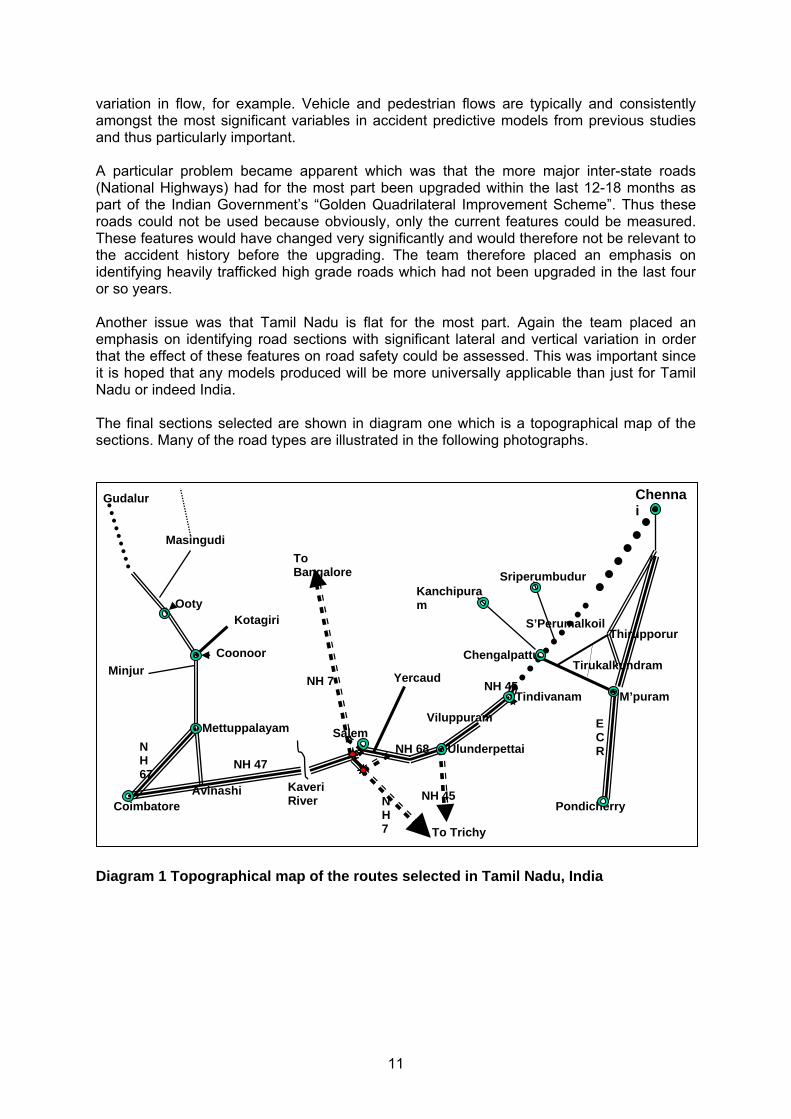
variation in flow, for example. Vehicle and pedestrian flows are typically and consistently amongst the most significant variables in accident predictive models from previous studies and thus particularly important. A particular problem became apparent which was that the more major inter-state roads (National Highways) had for the most part been upgraded within the last 12-18 months as part of the Indian Government’s “Golden Quadrilateral Improvement Scheme”. Thus these roads could not be used because obviously, only the current features could be measured. These features would have changed very significantly and would therefore not be relevant to the accident history before the upgrading. The team therefore placed an emphasis on identifying heavily trafficked high grade roads which had not been upgraded in the last four or so years. Another issue was that Tamil Nadu is flat for the most part. Again the team placed an emphasis on identifying road sections with significant lateral and vertical variation in order that the effect of these features on road safety could be assessed. This was important since it is hoped that any models produced will be more universally applicable than just for Tamil Nadu or indeed India. The final sections selected are shown in diagram one which is a topographical map of the sections. Many of the road types are illustrated in the following photographs.
Diagram 1 Topographical map of the routes selected in Tamil Nadu, India
Coimbatore
Salem
Ooty
Coonoor
Mettuppalayam
Gudalur
Yercaud
Chennai
Viluppuram
Tindivanam
Kaveri River
Kanchipuram
M’puram
Kotagiri
Chengalpattu
Pondicherry
To Bangalore
Tirukalkundram
Thirupporur
Avinashi
Sriperumbudur
Minjur
S’Perumalkoil
ECR NH 68
NH 45
Ulunderpettai
To Trichy
NH 47
NH 45
NH 7
NH 67
Masingudi
NH 7
12
Figure 1 Mountain roads with tight bends and steep hills, both high (left) and low
(right) volume
Figure 2 Medium volume rural dual carriageways
Note: Many examples of this road type were recent construction and thus unusable for the project.
Figure 3 Medium volume rural single carriageway roads
13
Figure 4 Upland plateau roads with low traffic levels, often tea estate roads
Figure 5 Low volume rural roads in flat terrain, with 1 and 2 lanes
Figure 6 Very high volume urban roads, divided and 2 lanes
(undivided and up to 6 lanes also used)
14
Figure 7 Medium volume urban roads, divided (undivided roads also used)
Figure 8 Urban roads with very high levels of side friction
2.1.2 Tanzania Road Surveys The terrain around Dar es Salaam is hillier than that around Chennai and the roads also have more curvature. Nevertheless, it was decided to travel north from Dar es Salaam to identify roads with high vertical curvature and gravel roads with medium traffic volume. As a result of this trip, a wide variety of road types were seen and included in the road list. Video footage was taken of many of them. Some roads were not included as the traffic volume was felt to be too low to be of use. The list included the following road types and the road sections finally selected are given in Appendix B:
15
Figure 9 Mountain roads with tight bends and steep hills, with low traffic volume
Figure 10 Upland plateau roads with low traffic levels
Figure 11 High volume urban roads, both divided and undivided, with and without
kerbs
16
Figure 12 Medium volume urban roads, both divided and undivided, with kerbs and side drains
Figure 13 Medium volume rural roads, both flat and straight and hilly and curved
Figure 14 Medium volume rural roads, both flat and straight and hilly and curved
17
Figure 15 Urban roads with low levels of side friction
Figure 16 Medium to low volume gravel road
A list of 14 road lengths, between 3 and 40 km and totalling 280 km, was agreed with the project partner. Useful data from a total of 263 km was received.
2.2 Data Components Since relatively little research has been carried out on the modelling of accidents in low-income countries, there was considered to be a need to collect data relating accidents to as many variables as possible to determine which that might have the greatest influence on accident occurrence. At the same time constraints on the project resources meant that the data collection exercise needed to be practical and cost effective. For most road safety statistical modelling studies, three distinct types of data need to be collected:
4. Accident data 5. Road environment inventory/survey data 6. Traffic flow data
These will be discussed in order in the following sections.
18
An initial decision was made about the way in which the dependent variable, namely accident numbers, would be collected for modelling with the other variables. This was that they be assigned to/within one kilometre sections, and this would therefore set the sectioning for other geometric variables which would be ‘averaged’ over these 1km sections. The reasons for this were as follows:
• The study is investigating the relationships between accidents and the overall nature of the road, rather than the reasons for accidents at specific sites or ‘blackspots’;
• Finding relationships would be much easier using a relatively short standardised
section length since features can “average out” over longer distances; • The analysis methods that were proposed to be employed are relatively coarse and
more suited to longer lengths of road (i.e. sections) rather than individual sites; • From experience it was felt unlikely that accident reports would describe the location
of accidents with sufficient accuracy to enable them to be logged to a smaller road length than this;
• In most cases the nature of a road does not change significantly over a kilometre
length, although the shoulder, for example, might vary considerable in some urban areas
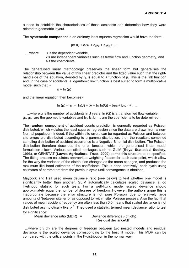
It was realised that the presence of blackspots within particular kilometre sections might serve to weaken general geometric relationships; however, it was felt likely that if specific engineering features were indeed largely responsible for creating such a spot, then these would still be reflected in any model produced. In the statistical technique of Generalised Linear Modelling (GLM) it is accepted that it is impossible from a practical point of view to explain all the variability in the data. Unexplained variability is expressed in the constant value (k). For many lengths of road studied in Tanzania, notably in the more urban areas, the road section between two defined points did not comprise a whole kilometre. Thus at the end of a road length the terminal part-kilometre section, has had its data proportionally adjusted in order to facilitate consistency in the analysis.
2.3 Accident data It was assumed that knowledge of the circumstances and severity of accidents would be essential in their modelling since the causes of, and countermeasures to help prevent, different accident types may be very different. For example, causes and countermeasures for a slight pedestrian accident would certainly be different to a major head-on vehicle-vehicle accident. The following data were therefore identified and proposed for collection from files at individual police stations.
• Road reference (in order to assign the accident to the correct section/kilometre) • Accident location, using whatever method is appropriate for the country, e.g.
coordinates, chainages, kilometre marker posts • Time of day of collision • Date, month and year • Overall accident severity (classified as that of the most severely injured casualty) • Number and types of vehicles involved
19
• Number, severity (fatal, serious, slight) and type (driver/rider, passenger, pedestrian) of casualties involved
• Vehicle type in which (or by which) the casualty was injured • Collision pattern: vehicle manoeuvres prior to crash: text and diagram. This is
especially important for junction accidents. Sketches were to be encouraged and collected separately if the appropriate movements could not be entered into a spreadsheet as compass directions for example.
• Collision type (e.g. head on, rear-end, pedestrian etc.) • Police reference code for the individual accident • Accidents which are located within 50 metres of a junction on any leg would be
defined as junction accidents and the distance from the junction was required if possible.
For reasons of practicality, statistical validity and in order to minimise the problem of including accidents which occurred at times when the nature of the road and the traffic might have been significantly different, the collection of the most recent complete five-year period for which accident data were available was requested if this was possible. The under-reporting of accidents is a well known and quoted phenomenon. It is often particularly acute in poorer countries where the traffic police may be very resource limited, and particularly in rural areas where it is often more difficult for police to attend the scene of an accident. It was beyond the scope of this to study to investigate under-reporting, and the assumption had to be made that this feature is, at least, consistent from year-to-year. However, if a relatively reliable measure of underreporting has been determined in a country, then obviously the predicted accident numbers from models can and should be adjusted to allow for such a level of under-reporting. If no measured estimate of underreporting exists, a proxy method which assumes that the severity ratio of different accident types should be reasonably consistent whatever the country can be used to give some measure of correction. This is based on the reasonable assumption that fatal accidents are much more reliably reported than slight accidents. It was considered that owing to the known unreliability and lack of detail in centralised records, that adequate accident data could only be gathered by visiting all the police stations covering the selected roads and examining the original accident reports. This was often complicated by the fact that in some cases, the reports were archived after a fixed period. In addition, more recent accident reports can often be missing from central filing systems if they are required for legal purposes in on-going court cases. The extraction of such data from original accident reports would be a major activity by the project partners.
2.3.1 Accident data - India Although kilometre posts and 200m stones have been installed on national highways, state roads and even fairly minor local roads, police accident reports tend to continue to use an ad hoc system of relating each accident to landmarks such as junctions, factories and bridges for many but not all reports. Therefore the project data collection teams had to relate each accident site from the police location descriptions using strip maps developed for the roads in order to locate it within the correct kilometre as defined by the kilometre posts. In some cases the data collectors visited individual accident sites as described on the police form in order to assign the report to a specific kilometre. In some cases the project team asked the accident data collectors for data for roads for which they did not have strip maps prepared which complicated the process. The police in Tamil Nadu did not use a formalised accident report pro forma. Thus the details required for this study had to be extracted from police “dockets” which tended to be rather
20
variable in their detail and which made the task difficult. IRT used their existing accident data collection pro form which they had used in previous accident data collection exercises and this is included as Appendix D. IRT also informed the project team that the police did not generally keep accident report forms for more than 3 or 4 years. For the above reasons IRT were not able to collect 5 years of data but were able to collect 3 years of data from 2002 to 2004 inclusive.
2.3.2 Accident data - Tanzania After discussion with national traffic police officers, the following procedure for collecting accident data was planned: • Visit police stations or regional headquarters to obtain original accident reports • Examine police accident reports to identify all the accidents which may have occurred
within the road sections during the defined time period • Use the accident reports to locate the actual accident site as accurately as possible • If the accident occurred within the road sections, record its coordinates using the GPS
device • After recording the coordinates of the start and finish of each kilometre section,
graphically identify in which kilometre section each accident occurred Three years of accident reports were examined for rural roads but, because of the large numbers of reports, only two years of accident data were examined for many of the busier roads in Dar es Salaam. The accident data collection team were given the instructions included as Appendix D to specify the precise information that it was considered should be extracted from the police records
2.4 Road environment inventory/survey data The nature of the road environment is known to have a major influence on the occurrence of accidents. The starting point for the collection of road feature data was to produce lists of various parameters which had been found to have a significant influence on road safety from existing research. These studies have been summarised in the literature review in Appendix A. Although a large number of variables can be collected during a physical survey of the road and it is desirable to measure as many variables as possible, this must be balanced against what is practical and feasible given time and budgetary constraints. From the significant variables highlighted in the literature review, a consideration of how variables are collated and used by HDM4, and also knowledge of the road and traffic that the project team expected to find in India and Tanzania, the following data were identified for collection: -
• Road reference • Location of section, using whatever method is appropriate for the country, be this
coordinates, chainages, kilometre marker posts • Median type and presence of gaps in the median • The number of side accesses • Carriageway surface type • Carriageway surface condition • Number of lanes and their widths
21
• Shortest sight distance • Whether or not curves are super-elevated • The presence of a slick surface • The presence and quality of road signs and road markings • The nature (type, width, condition) of the shoulder, divided into two zones since
many roads have, for example, a narrow sealed strip and a wider unpaved area, both of which are used by vehicles as a refuge and therefore worth recording
• The presence and quality of a footpath • The degree of side friction imposed by pedestrians, shop fronts, parked vehicles,
bus stops on passing traffic • The nature of the off-road environment (embankment or flat; rural or urban;
residential or industrial; drains, barriers or kerbs; etc) • A sketch of the road cross section to support the above data
For most of these variables an average value can be determined during a brief stop near the end of the section (note that some of the variables are relatively subjective), although a few variables need to assessed, measured or counted over the entire section (e.g. number of side accesses, shortest sight distance). It was, however, found to be sufficient to drive over each road section only once in order to carry out the complete road survey. In order to allow the project to establish universal relationships between accident rates and other variables, it is necessary to identify roads which show wide variability in all the above variables. Ideally separate kilometre sections would be chosen across the entire road network to encompass the full range of all variables. However, this was both impractical and expensive, so site selection was initially based on lengths of approximately 10 kilometres on a variety of roads with variation in, for example, surface type or traffic volume from one length to another, but that there was also variation of features like curvature or side friction within each length. Establishing a list of road lengths to be surveyed and upon which the project would depend for successful results was obviously a vital activity which occupied most of the first project visit to each country. Roads which significantly changed or been improved during the last four years were not selected for study since the accident statistics would not then relate to the current road environment that would be surveyed.
2.4.1 India: observations of road survey methodology After discussion with the project partner (IITM) to allow refinement of the required road survey data, a data collection form was produced, trialled and improved by the project team and partner. Detailed instructions were also issued to the local partners to assist them with filling in the various fields. Photographs were used to give examples of the various (subjective) levels (good to poor) to be applied to the objective measures such as side friction (level of encroachment of pedestrians and traders onto the road, poor parking etc.). The Instructions prepared for the survey teams together with a pro forma is given in Appendix E. As described above, kilometre posts are present along most roads in the list (and even 200m markers stones in many cases). These allowed the road lengths to be easily divided into kilometre sections
22
2.4.2 Tanzania: observations of road survey methodology The most significant observations during the visits to Tanzania and changes made to the data collection methodology are described below. An important difference between the Indian and Tanzanian road networks is that the latter has no formal system of kilometre posts, beyond those left behind by contractors and which often bear no relation to the chainage and coordinate system operated by TanRoads, which itself was seen to be inaccurate in places. Since identifying the exact start of a road length from the coordinates of a node and an odometer reading over 10-20 km may incur errors of several hundred metres, it was decided that the coordinate system of TanRoads would not be used and that the data collection team should set up their own coordinate system. This would entail the team driving to the intended start of the road length and then along the length in order to find the coordinates of the start and end of each kilometre section, studying the police reports to find the coordinates of each accident, and then graphically identifying in which kilometre section each accident occurred. The data collection form used in India was further trialled and refined and a set of detailed guidance notes was written (Appendix F). Collection of the specified data was found to be reasonably straightforward. A set of photos on laminated cards, illustrating a wide range of variables, was also given to the data collection team to improve the consistency of subjective data. This type of guide was initially prepared for the India team and proved to be particularly helpful, and so an improved guide was produced for the Tanzania surveys (see Appendix G). Although all road lengths were divided into kilometre sections, some urban sections were recorded with different lengths. Roads defined between junctions are rarely a whole number of kilometres, thereby leaving a part-kilometre section at the end. Corrections were made for this in the dependent variable (accident) data values.
2.5 Flow Data Flow data is potentially critical to the success of the project since this tends to have the most significant influence on accident occurrence (as it increases exposure to risk for the individual road user). Associated variables of traffic volume are traffic mix, and its speed, and in developing countries there tends to be a high proportion of non-motorised traffic including animal carts and pedestrians and also the presence of types of slow-moving motor vehicles (e.g. motorised rickshaws). Thus, as a consequence the mean speed of traffic tends to have much wider variance than in developed countries, which is likely to be another contributory factor in accidents. Ideally flows within each Kilometre section would be measured, but this was not feasible due to time and financial constraints. Thus the following data were requested:-
• At one point on each road length: • the traffic volume throughout a 12-hour day grouped into appropriate categories • the speed of freely moving light vehicles at intervals during the day, taken at a
representative location along the length, (minimum of 100 vehicles measured). • the pedestrian volume throughout the day both walking alongside the road and
crossing the road (within a measured length, typically 50 metres), grouped into adult and child
• At each major junction:
• the traffic volume throughout the day grouped into appropriate categories
23
• the pedestrian volume throughout the day walking both alongside the road and crossing the road, grouped by direction and by adult/child, male/female
2.5.1 India: Flow counts To maximise the number of flow readings which can be taken a sample of 24 hour counts were made and were used to factor up a larger number of 12 hour counts. Count locations have been distributed across the road lengths selected in order to maximise coverage. They were made more frequently where there was expected to be changes in the numbers, i.e. nearer or in settlements. An assumption was made that flows would not vary greatly over long rural distances, thus counts were made less frequently in these sections. The number and location of counting stations for each of the study sections given in Appendix B was agreed with the local team.
2.5.2 Tanzania Flow counts Some roads in Dar es Salaam have two to three lanes in each direction, wide median and large tree-lined drains between the road and the footpath. Pedestrian counting along these roads required extra observers. For this and other similar reasons and because data collection costs generally appear higher than in India, it was necessary to reduce the number of vehicle categories to be counted. Thus traffic was counted in the following four categories.
Another way in which costs were minimised was by reducing the duration of some counts to 12 hours. Most count sites were specified as being at the mid-point of the road length, although in some cases (often in urban areas), sites were specified as being between two major junctions. For similar reasons, pedestrian counts were grouped into only adults and children; and no distinction was made between male and female.
2.6 Curvature data Reduced sight distances are known to affect accident rates. Although reduced sight distances can be identified during a road survey, the assessment can be either time consuming or subjective. For the following reasons, it was decided to use the track function of a GPS device to measure the vertical and horizontal curvature of the roads under survey: • Vertical and horizontal curvatures of a road are the main reasons for reduced sight
distances. • It was known that the track function of a GPS device is able to record data from which
total vertical displacement, number of crests and total swept angle can be calculated. These values are used during it other analyses in HDM-4.
• The data collecting teams were loaned GPS devices for possible use in checking accident location and survey location
It was therefore anticipated that the GPS devices would be used to record tracks along all road sections, and that curvatures would subsequently be calculated from the recorded data.
24
It was expected that this activity would involve little more than fixing an antenna to the roof of the survey vehicle, and recording a waypoint at the end of every kilometre section during the road survey in order to divide the track record into kilometre sections.
2.6.1 Curvature data recording in India and Tanzania Tracks were recorded with the GPS device as planned, although it was ultimately found that the data were not of sufficient completeness or accuracy to be included in the analysis. In particular, the vertical curvature of near-flat roads was often lost during ‘drift’, whereby the measured position of a static device changes gradually, an effect which has little impact on horizontal curvature but great impact on vertical curvature.
2.7 Junction survey data Although the focus of the project has tended to be on road lengths, perhaps because HDM4 is more likely to be used for long road improvements than for smaller urban upgrading projects, it is known that a significant percentage of accidents, particularly in developing countries, occur at junctions. The project therefore intended to collect accident and other data at junctions. The collection of data relating to accidents which occur at junctions and other variables such as traffic flows are described in other paragraphs. The following data specifically relating to the environment of the junction was therefore identified for collection: • Junction type • Number of legs • Width and number of lanes on entry and exit on each leg • The angle between the centre line of each leg • Whether any leg has a gradient • Whether the junction itself is on a gradient • Whether any leg is curved on entry or exit • Whether any leg enters the junction with an offset • Whether there are visibility restrictions for traffic emerging from a leg • Whether there are visibility restrictions for traffic approaching on a leg • The dominant route or flow through the junction, if present • The presence of pedestrian islands between the entry and exit of each leg • The type of control – traffic police, lights – and whether the control is obeyed • The speed limit through the junction • The presence of pedestrian crossings across the legs or the junction • The presence of filter lanes for left and right turns • The presence of warning and information signs on entry to the junction • The presence of parking areas, formal or informal, close to the junction
2.8 Works history data Although the accident data collected was restricted to the most recent three-year period for which accident data is available, it remained possible that the nature of the road changed during this relatively short period. It was therefore specified that a brief summary of the works carried out on each road during the accident record period should be recorded. The local partners in each country were responsible for using their professional contacts within the road authorities to produce this summary of works.
25
3 Results: Compilation of data The main hypothesis was (i) that the accident models can be developed to explain and identify key factors and their relative importance on accident rates and, (ii) that relatively simple adjustment methods can be developed so that the models can be implemented immediately in HDM-4. It was considered that this would provide a reasonable compromise of achieving acceptable predictor accuracy without the need for large-scale, difficult studies in any country that is using HDM-4, in order to obtain detailed information without which the safety component could not be used.
3.1 Roads sections, India In Tamil Nadu, the original aim was to survey and obtain accident data for 1000km of road. After costing various tasks associated with obtaining the inventory, flow and speed and accident data this had to be reduced to about 570km. There were considerable mismatches between stretches of roads for which there were survey data and those for which accident data were supplied. This was due chiefly to a misunderstanding between the local partners whereby they failed to communicate adequately. Thus a subsequent exercise was carried out by the local team to survey further sections of road to improve the correspondence of data, since this was less onerous than the tasks entailed to obtain accident data. However, additional accident data were obtained for one stretch of road (East Coast Road section 24). These adjustments meant that data for 492km of road were ultimately available for the analysis and these are listed in Appendix B. In Tamil Nadu, 3 full years of accident data were available for all road sections (from 2001 to 2003 inclusive). There are several major difference between the surveys carried out on the roads in Tanzania and those in Tamil Nadu. This is chiefly because the types of roads and aspects of the environment are significantly different between the two locations. In Tamil Nadu there were, for example, no unsealed roads which were major or strategic routes, no culverts and no provision of footpaths either beside or separated from the carriageway.
3.2 Roads sections, Tanzania A road survey was made of all the sections defined in Appendix B in approximately kilometre lengths. The road surveys were requested to be carried out between 8 am and 5 pm on a typical weekday. In practice not all of the 280 kms proposed sub-section were surveyed and in some cases accident data were not available or supplied. However, the survey data contains 264 kilometre sub-sections with complete information on variables such as: road widths, construction, condition, side friction, cross-section, footpaths, shoulder widths and condition, median between lanes etc. The data were assembled into worksheets for each sub-section. The road sections were defined by a start and end-point with a GPS position; the sections were divided into sub-section using way-points which were close to 1Km apart. The waypoint positions were generally supplied with a GPS reference coordinate.
3.2.1 Way-points Way-points which defined the start, mid-points and ends of road sections were generated with a GPS device. In theory these enabled accidents to be located within each road sub-
26
section, and so facilitated the linking of accidents to road sub-section. Way-points were also produced for the more major junctions, where junction details had also been recorded. The use of the junction way-point GPS data permitted the classification of accidents into either junction or non-junction. However, not all waypoint GPS data were available: the starting and ending GPS references were available for some sections, but not for all. Missing waypoint positions were estimated by plotting accident GPS references to give the ‘road shape’ and then calculating the likely waypoint position given the sub-section lengths used in the surveys.
3.2.2 Linking of data sources The linking of survey (inventory) data with accident data used the road section identifier and the waypoint reference (as defined by GPS data). The survey sub-sections as defined by the waypoints were the base unit. However, because of matching problems plus the fact that there were no accident data for section 20.1, the total of matched sub-sections was 264 for analysis purposes. There were 3754 accidents in total. . A section number and a ‘kmwithin’ number (which is the number of integer kms from the start of the section), and the GPS reference were used for matching. Junction GPS values were available and could be used to see if the accident was close to a junction. In practice matching the accidents to sub-sections did not work well, with only about 70% of accidents matched. However many of the seemingly matched accidents were clearly not in the correct sub-section, probably due to waypoint GPS errors or inconsistencies. The ‘kmwithin’ variable was used within a section to assign a waypoint, i.e. if the section was 5km long then there were 5 waypoints at 1km intervals. However, because ‘kmwithin’ is integer then this would not always be correct because the inter-waypoint distance varied. It was further complicated by some of the waypoints being numbered in reverse, i.e. some seemed to be numbered from the end of the section not the start. However, by using waypoint GPS data together with accident GPS data the waypoint reference was adjusted to cope with different sub-section (inter-waypoint) lengths. This was a manual exercise which required a graphical plot in some cases of the accidents in the section (with the waypoints). The resulting allocation of accidents to sub-sections is not perfect, but has provided a relatively good match. The count of junction and non-junction accidents by severity by sub-sections was then matched to the survey section data – giving 264 matches.
3.3 Preliminary simple analyses of raw data The main measure of interest is the number of accidents during the 3-year study period, (2001 to 2003). The accidents may be classified as one involving a fatality, a serious injury, a slight injury or damage only. The severity of the accident is determined by the highest casualty severity. The initial analysis has looked at the total number of accidents as well as the number of killed or serious injury (KSI) accidents. However the number of accidents depends very much upon the traffic flow. The total flow for 3 years of traffic between 8:00am and 8:00pm was computed and used as either an off-set or a modelling variable. (Using the flow as an off-set assumes that the flow value is used to model a rate per 100M vehicle Km. On the other hand using the flow as a variable in the model assigns a parameter value to flow allowing for the fact that the relationship between number of accidents and flow is non-linear.) The flow used was the total of all mechanical vehicles during a 12-hour period.
27
Although the relationship between number of accidents and flow is non-linear, it is still informative to examine the accident rate per 100M vehicle Km and this was calculated using the following function:
Define the total flow per kilometre for the period of reporting per 100 million vehicles as Q, where: Q = 365 x (number of years of accidents) x (Sum of all motorised vehicle flows) x (length of road Km) / 100,000,000 and accident rate per 100 million vehicle kilometres as R, where: R = (Accidents in reporting period) / Q
The rate (R) was calculated for: • the total number of accidents, • the number of non-junction accidents (i.e. not near a known and major junction), • the total number of killed or serious injury accidents (KSI) • the number of KSI accident not near a junction
These have been analysed by road inventory factors. The initial analyses looked at the average rates for each factor level in turn. Factors interact with one another and hence a more complex analysis is also required in order to obtain a better understanding of what factors influence accident rates, for example the lane width may be important as may the side friction but only by including both factors can this be taken into account.
3.3.1 India: Preliminary Analysis by Individual Road Factors Accident rates were calculated for each section of road which constituted a complete continuous length that had been surveyed (Table 1). Figures for both all personal injury accidents (PIA) and those involving victims who were killed and/or seriously injured (KSI accidents) are shown separately. The accident data in India did not allow for accidents to be assigned to particular junctions within each kilometre sample length and there is some doubt about how well this aspect of the accidents was recorded. Thus analysis has been performed on all accidents irrespective of whether they were listed as being at or away from a junction. The rates for the different sections are highly variable, in most cases the KSI rates follow the PIA rates but not in all cases.
28
Table 1 Average all accident and KSI accident rates by road section Survey section
In Tamil Nadu there were four major road types identified by the partner organisation. These classifications were defined chiefly by the level of the highway authority responsible for construction and maintenance. This method of classifying the roads corresponds to that used in the HDM-4 model which has been developed for use by maintenance engineers and ministry of transport personnel. The road classes were:
National Highway (NH): major inter regional roads maintained by Central Government State Highway (SH): major intra-regional roads maintained by State Government District Roads (DR): less major routes maintained at the district level Hill roads: (HR): rural roads (included to give variation)
The average PIA and KSI rates for the separate road types are shown in Table 2 and in Figure 17. The table indicates that there are significant differences between the accident rates of the various road types. The highest rates occur on National Highways, followed by District Roads then State Highways, with the Hill Roads having the lowest rates. The relatively low rates that occur on the Hill Roads may be due to higher underreporting rates since these roads carry very low vehicle flows and are remote in nature. If the rates were low for this reason it might be expected that the ratio of KSI to PIA accidents would be higher since the higher severity accidents are generally more likely to be reported to (and recorded by) the police. However, Table 2 indicates that this is not the case, although it is possible that all accident severities are being equally underreported.
29
Table 2 Average rates within road types and total length sampled Road type
Average rate for all accidents
Average rate for KSI accidents
Total length (kms)
NH 173 89 261 SH 38 14 52 DR 99 47 146 HR 21 8 28
020406080
100120140160180200
NH SH DR HR
Acc
iden
t rat
e 10
0M v
eh/K
M
Average rate for all accidents Average rate for KSI accidents
Figure 17 Average rates for each road type for all and KSI accidents
As a preliminary review of the data the following analysis shows the average accident rates for particular features which had been logged or measured by the road survey. The first chart in each pair shows the total accident rates (all PIAs); the second shows the same information for KSI accidents. All PIA rates
0.0
50.0
100.0
150.0
200.0
250.0
Poor Fair Good
Road condition
rate
100
M v
eh/K
M
NH SH DR HR KSI Rates
0.00
20.00
40.00
60.00
80.00
100.00
120.00
Poor Fair Good
Road Condition
rate
100
M v
eh/K
M
NH SH DR HR
Figure 18 Accident rates by road surface condition In Tamil Nadu rates are generally highest where road surface conditions have been categorised as Fair, and are lower for Poor or Good conditions. The exception is the State Highway (SH) for which rates are best with poor surface conditions and get higher with improving condition. It may be possible that the State Highway road characteristics are more similar to Tanzanian roads (see later Section 3.3.2) than the other categories. It is not known how well the categories of Poor, Fair and Good correspond between the two countries. Patterns are similar for the plots of the total PIA accident rates compared to the KSI accident rate for the different road classes.
30
0
50
100
150
200
250
300
0-1 2-3 4-5 6-7 8-9 10-11 12+
No Public Accesses
rate
100
M v
eh/K
MNH SH DR HRAll PIA
rates
0
20
40
60
80
100
120
140
0-1 2-3 4-5 6-7 8-9 10-11 12+
No Public Accesses
rate
100
M v
eh/K
M
NH SH DR HRKSI Rates
Figure 19 Accident rates by number of side accesses There are no obvious patterns in the average accident rate with increasing numbers of public accesses along a road. In Tamil Nadu generally the number of public accesses along major roads particularly in the more urban areas is extremely high.
0
50
100
150
200
250
300
None Low Medium High
Side Friction
rate
100
M v
eh/K
M
NH SH DR HRAll PIA rates
0
20
40
60
80
100
120
140
None Low Medium High
Side Friction
rate
100
M v
eh/K
MNH SH DR HRKSI Rates
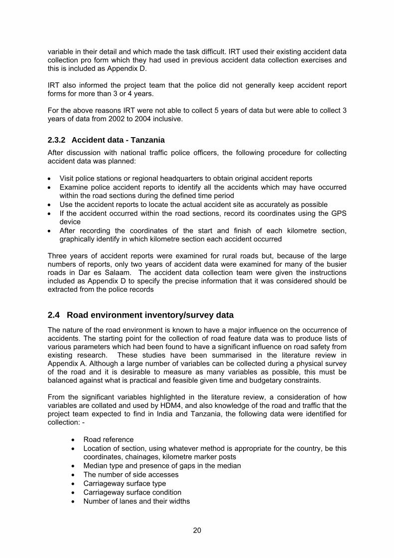
Figure 20 Accident rates by roadside side friction levels In Tamil Nadu accident rate increases with increasing side friction for the District roads and the State highway sections, this being more pronounced for the District roads at the highest side friction level. On the National highways, however, there appears to be a dip in the trend for Medium side friction levels. Again the pattern in all PIA accident rates is mirrored by the KSI rates.
020406080
100120140160180200
None Poor Fair Good
Condition of Signing
rate
100
M v
eh/K
M
NH SH DR HRAll PIA rates
0
20
40
60
80
100
120
None Poor Fair Good
Condition of Signing
rate
100
M v
eh/K
M
NH SH DR HRKSI Rates
Figure 21 Accident rates by condition of road signs Little can be inferred from Figure 21 with respect to the influence of road sign provision on accident rates for the various categories of roads, apart from possibly a slight indication of a
31
lower rate with improved signing. The differences in the distributions of the various states on the different road types are sporadic.
0
50
100
150
200
250
None Poor Fair Good
Condition of Markings
rate
100
M v
eh/K
M
NH SH DR HRAll PIA rates
0
20
40
60
80
100
120
None Poor Fair Good
Condition of Markings
rate
100
M v
eh/K
M
NH SH DR HRKSI Rates
Figure 22 Accident rates by condition of road markings Similarly from Figure 22 there are no clear consistent trends in the effect of road markings on accident rates within the sections of roads sampled for Tamil Nadu. The results shown for the District Roads may not be representative since most of the data has a value of either 'None' or 'Good'.
0
50
100
150
200
250
300
0.0 0.5 1.0 1.5 2.0 2.5 3.0+
Shoulder Width
rate
100
M v
eh/K
M
NH SH DR HRAll PIA rates
0
20
40
60
80
100
120
140
0.0 0.5 1.0 1.5 2.0 2.5 3.0+
Shoulder Width
rate
100
M v
eh/K
M
NH SH DR HRKSI Rates
Figure 23 Accident rates by shoulder width Again, the effect of shoulder width on accident rates for State Highway and Hill Roads in Figure 23 because the range of shoulder encountered was limited (none or 0.5M or 1.0M wide). In addition virtually none of the Hill Roads and most of the State Highways sampled had any shoulder, thus the figures illustrated are based on very limited data. Most of the District Road and the National Highway sampled had shoulder of 1.0 m, 1.5m or 2.0m width. Both data sets show that the rate is lowest for 1.5M provision of shoulder within this range which supports a finding from earlier research in other countries (see Hills, Baguley and Kirk, 2002).
3.3.2 Tanzania Preliminary Analysis by Individual Road Factors Accident rates per 100 million vehicle kilometres were derived for each road sub-section. As discussed above in Section 3.2, there were 264 sub-sections where data were available and had been matched, thus all analyses are based on this sample. An initial analysis was conducted to see how these rates changed by factor level. For example the average rates (all accident and all KSI) per road section are shown in Table 3, though as discussed above, not all of the road sections contained as many sub-sections as originally planned.
32
Table 3 Average all accident and KSI accident rate by road section
10.1 Morogoro Road 10 308 192 10.2 10 76 49 10.3 10 102 54 10.4 10 79 48 11.2 Chalinze to Segera 15 227 101 11.3 10 185 158 13.1 Segera to Tanga 10 146 113 13.2 10 139 112 14.1 Tanga to Horohoro 40 301 216 18.1 Serega to Mombo 10 125 94 18.2 20 303 171 19.1 Mombo to Lushoto 25 206 140 20.1 Lushoto to Mlalo No accident data 23.1 Ikwiriri Road No survey data 23.2 10 132 72 23.3 10 475 419 23.4 10 699 615 24.1 Mkuranga to Kisiju 10 546 334
It is clear from the table that there is considerable variation between the average rates per 100m veh/km per section; and it is reasonable to assume that some of this variability can be explained by the road factors measured in the road survey. Road condition and number of side accesses are two factors which could be related to accident rate, Figure 24 shows a plot of the rates by the different factor levels. It clearly suggests that the poorer the road surface condition the higher the accident rates and generally the more side accesses the higher the accident rates.
33
0
100
200
300
400
500
good fair v poorsurface condition
rate
100
M v
eh/K
mall accs ksi accs non-junct non-junct ksi
0
100
200
300
400
500
600
0 1 2 3 4 5+side accesses
rate
per
100
M v
eh/K
m
all accsksi accsnon-junctnon-junct ksi
Figure 24 Accident rates by surface condition and side accesses In practice most of the roads have good surfaces (n=204) whereas only a few (n=10) have very poor surfaces – so, although this may appear graphically to be a strong and consistent increasing relationship this factor did not prove to be statistically significant in the accident model (later section). Similarly, the number of side accesses also appears to be a fairly straightforward and consistent relationship, but in fact most sub-sections had no side accesses (n=109) and only a few (n=23) had more than 5 side accesses. Thus this comparatively small sample size resulted in this factor also not being statistically significant. Nevertheless, it is felt that this situation would be different, i.e. these two factors may prove to be important and reach increased statistical significance if more data points were available. It is apparent that the Tanzania data behaves broadly similar to that of the State Highways in India, in that there is a general increase in accident rate with increasing number of accesses along a road. There was a greater number of public accesses recorded on the road stretches in India compared with Tanzania, perhaps reflecting the greater density of the population. There was no median separation on most of the sample road sections (n=222, i.e. 85%) in Tanzania. Only 1 sub-section had road studs and the others were described as wide and low, and were open or had trees. There were not, therefore, sufficient data to reach any conclusion about the effect of the median on accident rates, although the single section with studs did had low accident rates. Accident rates by side friction (for paved and unpaved roads) and footpath location are shown in Figure 25. There is little difference between ‘no side friction’ and ‘fair friction’, but as the level of side friction increases (i.e. becomes worse) then the accident rates increase. Most footpaths were next to the traffic (67%) which is safer than having no footpath (or none recorded) but for KSI accident rates it appears to be as safe for the footpath to be separated
0
100
200
300
400
500
noneunpaved
nonepaved
fairunpaved
fair paved moderatepaved
poorpaved
friction
rate
100
M v
eh/K
m
all accs ksi accs non-junct non-junct ksi
050
100150200250300350400
missing data next to traffic away from traffic
footpath
rate
100
M v
eh/K
m
all accs ksi accs non-junct non-junct ksi
Figure 25 Plot of accident rates by side friction and footpath
34
usually by a narrow strip of land from the carriageway. Accident rates by road signs and road markings are shown in Figure 26. There appears to be little difference between accident rates for ‘good’ and ‘fair’ road signs but the rates are generally higher where there with no signs, i.e. having a sign appears to be beneficial. However, the situation with road markings is more complex, in that the plot is denoting good markings having a low accident rate, whereas poor or even fair markings are associated with higher rates. The interpretation is complicated by the fact that markings are probably only used where there are junctions and so no markings refer to non-junction sub-sections which, without the associated traffic turning movements, are likely to be safer than sub-sections with junctions. Given that the standard of road signs and road markings will vary within a kilometre section, then a clearer picture may have emerged if each sign had been rated separately and somehow associated with nearby accidents. However, there are clear organisational as well as analytical problems in attempting to disaggregate the data, and so using an average standard within the section was the best compromise, albeit not providing a very clear result.
0
50
100
150
200
250
300
350
400
450
good fair none
road signs
rate
100
M v
eh/K
m
all accs ksi accs non-junct non-junct ksi
0
100
200
300
400
500
good fair poor none
road markings
rate
100
M v
eh/K
mall accs ksi accs non-junct non-junct ksi
Figure 26 Accident rates by road signs and road markings Accident rates by road lane width and shoulder width are shown in Figure 27. There appears to be some indication of lower accidents rates being associated with wider road lanes; however, it is not a clear relationship. Accident rates where there is no shoulder on unpaved roads tend to be high, with an improved safety benefit where there is a shoulder. However, for the widest shoulder, accident rate increases, and this may be due to drivers using the wide shoulders thus increasing their accident risk on this non-road surface. The graph suggests that a paved road may have an optimum shoulder width of between 0m and 2m, and wider shoulders are associated with higher accident rates.
Figure 27 Accident rates by road lane width and shoulder width
35
4 Results: The Modelling Approaches The number of accidents and the accident rate per 100 million vehicle kms have been investigated by looking at average values across single factors above. It is likely that these are interrelated and so the following analysis examined and identified the key influential factors simultaneously. Four different approaches have been considered.
1. The use of Generalised Linear Modelling (GLM) models developed in high-income countries was considered to be a worthwhile starting point. As possibly the most comprehensive set of models for different road and road intersection types has been developed in the UK, and have all been incorporated in a single software program called SafeNET, it was proposed that this software should initially be tried using only the parameters recorded in the two trial countries that SafeNET demands.
2. 3.
1.2. A GLM approach using all data collected. Total accidents over three years (normalised for some roads in Tanzania where only 2 years accident were available) and KSI were modelled. The flow of total motorised traffic over the reporting period calculated from observed flow data in a 12-hour period has been used in the model as an off-set. Models have been fitted under the assumption that accidents are Poisson distributed. The over-dispersion of the variance relative to the mean has been handled by using a model scale parameter estimated using (Deviance/Degrees of Freedom).
2.3. Australian model approach. This approach derives the base accident rate per million
vehicle Kilometres, and factors are used to estimate the rate for roads or conditions that differ from the base condition, i.e. if the base is for a straight road then road curvature factors will apply for non-straight roads.
3.4. A hierarchical regression tree approach. This approach uses a hierarchic decision
tree to identify the key factors that influence the number and/or rate of accidents. In this way homogeneous groups of accidents are identified which can be used to estimate accident risk.
4.1 Trial of SafeNET Models SafeNET 2 (Software for Accident Frequency Estimation for Networks) is an interactive and innovative software package that was produced by TRL to assist traffic engineers, transport planners and road safety officers in the design of safe road networks. The software allows estimates to be made of the number of personal injury accidents per year for particular elements of a road network (road sections and junctions of different types). It is relatively quick and easy to use and tends to be utilised for assessing the safety of a traffic management scheme. It is based on numerous UK road accident models that were developed chiefly by TRL over a period of about 15 years from specific studies of different road types and junctions. Each study involved the collation and analysis of an extensive database at hundreds of sites on the UK network. Although it could be argued that owing to the very different traffic and road conditions existing for other countries, and certainly developing countries, such models would be
36
inappropriate, a trial of the application of SafeNET was considered worthwhile to determine whether simple correction factors might be sufficiently reliable to utilise this existing software package. SafeNET treats each road section or junction individually and the total number of accidents in the network is predicted as a sum of estimates of each element. Up to four models with different levels of sophistication are included for each of a number of different link and junction types. The simplest models predict the number of vehicle collisions (with other vehicles or objects) and also pedestrian accidents, whereas the more detailed models predict the number of accidents in different categories (e.g. single vehicle, tight-turning, etc.). However, the latter require input of different design features of the junction or road, such as gradient and traffic signal timings, but might in turn be expected to give more accurate predictions. However, the available data from India and Tanzania and SafeNET’s available models dictated that the program was run with selection of either Composite Urban Roads (meaning a combination of single and dual carriageways) or Interurban (Rural) Single carriageway sections. As in most accident models, traffic flow is the main predictor variable, and thus the data were sorted into sections which in this respect could be regarded as ‘homogeneous’, i.e. a length of road over which a total traffic flow measurement applied and values for any other variables required by SafeNET could be reasonably averaged. Also, as the SafeNET models have been standardised to use AADT flows, correction factors were applied to convert the 12-hour counts obtained in India and Tanzania to 24-hour flows. A comparison of results is shown in Figure 28 to Figure 31 where the accident numbers (actual and predicted) have been plotted against total 24-hour flows (the main explanatory variable). It can be seen that for the range of traffic flows experienced on the study roads, the differences between actual and predicted accident numbers for both Tanzania and India are quite wide with actual recorded accidents generally being higher. This is despite the known fact that much higher levels of underreporting of accidents tend to be prevalent in developing countries than in the UK. It may be noticed from the figures that there appears to be more concordance within the urban situation compared with the rural model. However, the mean difference between actual and predicted accidents per kilometre in urban areas was 7.5 in India and 32.1 in Tanzania. These relatively large differences (for a single kilometre) had particularly high standard deviations of 19.1 and 14.5 respectively. For the rural sections the mean difference between actual and predicted accidents per kilometre was 8.2 and 2.3 for India and Tanzania respectively. For India this had a correspondingly high standard deviation of 8.7 for India, though for Tanzania this was 0.9.
SafeNET predicted accidentsActual no. recorded accidents
Figure 30 Tanzania data: Accidents per 3 yrs by Traffic Flow
{URBAN SafeNET model}
0
5
10
15
20
25
30
35
40
45
50
55
60
65
0.00 1.00 2.00 3.00 4.00 5.00 6.00 7.00
24 hrs Traffic Flow (x 1000)
No.
of i
njur
y ac
cide
nts
in 3
yrs
SafeNET predicted accidentsActual no. recorded accidents
Figure 31 Tanzania data: Accidents per 3 yrs by Traffic Flow {URBAN SafeNET model}
39
4.1.1 SafeNET Conclusion It was concluded, therefore, that due to these rather irregular variations obtained between actual and predicted values, it would be neither valid nor useful to apply simple multiplication factors or even devise more complex conversion formulae to the SafeNET output. This is principally because, probably due to the many wide differences in traffic mix, road quality, design and road user behaviour, these results indicate that the simple application of SafeNET in developing countries would not yield sufficiently trustworthy predictions of accidents.
4.2 Generalised linear modelling trials The SAS GENMOD procedure was used for this analysis (Statistical Analysis System – GENeralised MODelling – SAS, 2005). The accident data were assumed to be Poisson distributed and a log link function was used in the model. The over-dispersion (over that expected from a Poisson distributed variable) was handled by using a scaling factor derived from the ratio of deviance to degrees of freedom. The Chi-squared values and tests were automatically adjusted. Generalised linear modelling was used and included a log link function that transforms the data such that the residual ‘noise’ can be assumed to be Normally distributed. The models fitted have the following form:
log(Accidents) = k log(Q) + ( ΣbiXi )
Where Q is the traffic flow for the accident reporting period, (either 2 or 3 years), Xi are modelling variables and k and bi are parameters to be estimated. Note: if Q is fitted as an off-set (as was assumed) then k is assumed to be unity.
This is equivalent to: Accidents = a Qk exp( ΣbiXi )
4.2.1 India: GLM modelling The flow was computed for 100 million vehicle kilometres for the period in which accidents were collected. The log of flow was input as an off-set in the model – thus the model was fitting the accident rate per 100 million veh/km. There were four roads types relating to National highways (n=244), State highways (n=101), District roads (n=86) and Hill roads (n=61). Initial analysis of side friction by road type suggested that there were quite different accident rates per 100 m veh/km. This is confirmed by the following plot where the National rate is somewhat higher than for other roads apart from where there was high side friction (see Figure 32). The analysis approach tried a large number of different models. The objective was to produce a parsimonious model which was credible and useful in gaining an understanding of the different effects on accident rates. A number of different variables were used:
40
Friction by road type
050
100150200250300
National State District Hill
Road type
All
acci
dent
rate
none low medium high
Figure 32 India: Accident rate by Road type and Side friction
Side friction (none, low, medium, high) Road surface condition (good, fair, poor) Shoulder width Shoulder condition (none, fair, poor, good) Number of lanes (1, 2, 4) Numbers of curves (0, 1, 2, 3, 4, 5+) Road markings (none, fair, poor, good) Road signs (none, fair, poor, good) Road speed (as assessed from a limited roadside survey and coded into 6 groups)
It was clear from an initial generalised model analysis, which included the whole set of data, that the estimates were strongly influenced by the relatively large number of National Highway sections, and also that the models did not produce a very good nor credible representation of the data. Models which included side friction (and road condition) within road type were a little better but still did not generate good solutions. The final models reported were fitted for each road type separately. It was found that different combinations of available variables were required in different models. The models were fitted for the all accident rate and then applied to model the KSI accidents. It must be noted that some of the models are based on quite small samples: the National Highway data with a sample of 244km sections is reasonable but models for the other road types should be regarded as indicative.
4.2.2 India: National Highway model The following table shows the variables and the estimated parameters as used when modelling the National Highways. The all accident model explained 31% of the non-Poisson variation and the KSI model 37%.
41
Table 4 Generalised linear model Variables and estimated parameters for National Highways (defaults for model comparisons shown in bold)
3.0+m 0.0000 0.0000 The relative effect of each variable has been judged by comparing to a base model. The base model used was for low side friction, good road markings, 2-lanes and no shoulder (as indicated by the emboldened parameters). The percentage increase or decrease from the base model for each variable in turn (keeping the others constant) is shown in the following table. Table 5 Percentage change in accident rates for each variable for National Highways
Increasing side friction on National highways increases the accident rate slightly going from ‘low’ to ‘medium’ and large jump from ‘medium’ to ‘high’. Sections with good road markings have a lower accident rate than those with ‘fair’ or ‘poor’ markings. Somewhat surprisingly there was a small improvement in the total rates and a more significant improvement for KSI rates, where there were reported to be no markings. This is probably because other road conditions are also poor on these sections, and the lower rate due to a decrease in speed on these sections. This hypothesis is supported by the fact that KSI accidents are more greatly affected since the more severe accidents tend to be associated with higher speeds. The presence of shoulder almost always has a positive effect on accident rates, especially those of 1.0M or 1.5M. This was a result which was found previously by Hills, Baguley and Kirk SJ (2002) in their CaSE study. They also found as in this study that at greater than 1.5M the shoulder has a less favourable affect on accidents, although a marked decrease in accident rate is indicated at 3 metres or more. This estimate is based on a very small sample of sections and thus is not reliable. Sections of National road with 4 lanes compared to 2 lanes have a greatly improved accident rate, this being more marked for the KSI rate. For the most part the results for the models for National Highways are easily interpreted and patterns in the rate with different values of the factors included in the models generally make sense.
4.2.3 India: State Highway model The following table shows the variables and the estimated parameters as used when modelling the State Highways. The all accident model only explained 18% of the non-Poisson variation and the KSI model 13%, which are not very good fits.
Table 6 Generalised linear model: Variables and estimated parameters for State Highways (defaults for model comparisons shown in bold)
lanes 2 0.0000 0.0000 The relative effect of each variable has been judged by comparing to a base model. The base model used was for good road condition, good road markings and 2-lanes (as indicated by the emboldened parameters). The percentage increase or decrease from the base model for each variable in turn (keeping the others constant) is shown in the following table.
43
Table 7 Percentage change in base model for each variable for State Highways compared to the base state
As road condition worsens the accident rate also tends to worsen. However, for KSI accidents the situation is more complex in that the rate at ‘poor’ road sections is less than at ‘fair’ road conditions. This is probably a consequence of decreased road speeds due to ‘poor’ condition relative to ‘fair’. The accident rates for all accidents and KSI accidents are much increased on roads with ‘poor’ road markings relative to the base of ‘good’ markings. State roads with a single lane (these have an unsealed shoulder designed to facilitate passing between vehicles travelling in opposite directions) have much lower rates compared to those with 2 lanes (one in each direction). Again this is probably because vehicle speeds are lower on these single lane roads.
4.2.4 India: District Road model The following table shows the variables and the estimated parameters as used when modelling the District roads. The all accident model explained 22% of the non-Poisson variation and the KSI model 22%.
Table 8 Generalised linear model: Variables and estimated parameters for District Roads(defaults for model comparisons shown in bold)
width >0.0m 0.0000 0.0000 0 or 1 -0.4032 -0.6322 No curves >1 0.0000 0.0000
The relative effect of each variable has been judged by comparing to a base model. The base model used was for good road markings, no shoulder and only 1 or fewer curves (as indicated by the emboldened parameters). The percentage increase or decrease from the base model for each variable in turn (keeping the others constant) is shown in the following table. The road markings give a mixed picture which is difficult to interpret.
44
Table 9 Percentage change in accident rates for each variable for District Roads compared to the base state.
District roads - %
increase over base model
All accidents
KSI accidents
none -31% -32% poor 30% -5% fair -49% -70%
road markings
good 0% 0% 0.0m 0% 0% shoulder
width >0.0m -66% -73% 0 or 1 0% 0% No curves
>1 50% 88%
For District roads, there are decreases in the accident rate for sections of road with fair or poor road markings compared with good markings. This result is difficult to explain but as stated above, it may be that various states of this factor are aliased with other factors which were either not measured or are not significant and thus have not been included in the model. There is an increase in the rate where the road markings are poor compared with where they are good. There are large decreases in accident rate where a shoulder is present. Where the road has two or more significant bends or curves, the rate is increases significantly. The model results are difficult to interpret for road markings but otherwise the results seem to conform to expected patterns.
4.2.5 India: Hill Road model The following table shows the variables and the estimated parameters as used when modelling the Hill roads. The all accident model explained 28% of the non-Poisson variation and the KSI model 34%. Table 10 Generalised linear model: Variables and estimated parameters for District
Roads (defaults for model comparisons shown in bold) All
accidents KSI
accidents Hill roads (n=61) parameter parameter
intercept 2.8731 2.3820 good -0.2995 -24.9527* fair 1.1501 0.7691 road
condition poor 0.0000 0.0000
3 -0.0146 -0.1280 No. curves 4 0.0000 0.0000
* note this very large parameter is because there were no KSI accidents on good roads The relative effect of each variable has been judged by comparison with a base model. The base model used was for ‘good’ road surface with 3 curves recorded (as indicated by the emboldened parameters). The percentage increase or decrease from the base model for each variable in turn (keeping the others constant) is shown in the following table. However, because of the estimated zero KSI accidents the percentage change cannot sensibly be estimated for road condition, i.e. the base is zero.
45
Where road condition is fair compared with good, the total accident rate is very much elevated over 3 times higher), the rate is 35% higher where conditions are poor rather than good. Since there were no recorded KSI accidents on good roads, obviously no estimations of the affect of road condition on these accidents could be made. There is a very small increase in the all-accident rate where there were 4 curves compared with the proposed base of 3 curves. The elevation in KSI accidents was more marked, but there were very few KSI accidents recorded on these roads.
Table 11 Percentage change in accident rates for each variable for Hill Roads compared to the base state.
Hill roads - % increase over base model
All accidents
KSI accidents
good 0% 0% fair 326% - road
condition poor 35% - 3 0% 0% No. curves 4 1% 14%
The results in the modelling exercise for the hill road data are generally difficult to interpret. In addition the base model is unsatisfactory since only 2 of the factors tested appeared to have a significant association with accident rate. Hill roads were included because it was desirable to include a range of road types in the analysis. These roads tend to be lightly trafficked, thus the accident numbers available tended to be very small. However, the rates were generally low compared with the other road types tested. It might be expected that these roads might have low accident numbers but relatively high rates, which is not the case here. It is not anticipated that many users of HDM-4 will be applying the program to such minor roads. The actual rates for the base models for India are given below:
Table 12 Base Rate models for India
Actual Base rates: India Acc/100Mil veh KM
Acc/100Mil veh KM
All Accidents KSI Accidents National Highway 111.0 66.4 State highway 26.8 10.1 District Roads 286.3 139.1 Hill Roads 12.9 0.0
4.2.6 Tanzania GLM modelling The modelling variables initially considered for Tanzania were:
Side friction (poor/moderate/fair/none) Shoulder width (none/0-1m/1-2m/2+m) Footpath location (missing/next to road/away from road) Sight distance (0-25m/25-50m/100+m)
Median (none/studs/wide,low,open/wide,low,trees) Road signs (good/fair/none) Road markings (good/fair/poor/none) Cross-section (open/embankment/cutting/hill-side)
Lanes (2/4) Construction (paved/not-paved)
46
Variables: log (all motorised traffic flow in the reporting period)
Average car speed Number of public access roads Number of private access roads Width of lane (2.5/3/3.2/…)
General linear models were derived for each of four accident count types, i.e. all accidents, all KSI accidents, non-junction accidents and non-junction KSI accidents. All of the models included a variable for the traffic flow per 100 million vehicle kilometres, as described earlier. This was included as on off-set, i.e. in effect the accident rate per 100 million vehicle kilometres was the dependent variable being modelled. The factors and variables listed above were fitted and different models were explored. The final models fitted included the variables: side friction, road condition, paved or un-paved, road signs and shoulder width. Paved/unpaved was combined with the side friction and with the shoulder width factors to allow for an interaction between these variables. A table of the estimated parameters derived for each model is given in Table 17, the table shows the parameter estimate associated with each level of the modelled factors. In order to judge the importance of each factor the percentage increase or decrease over a base model was calculated for each factor in turn. The base model was defined as:
No side friction (for paved roads) A good road surface No (or missing) road shoulder (for paved roads) Good road signs
The impact of side friction at different levels is shown (for each model) in Table 13 for paved and for unpaved roads. It can be seen that there is generally an increase in rates for most models, especially when the side friction is described as ‘poor’. The increase is much larger for unpaved roads; however, there are very few sub-sections for unpaved roads with poor or moderate side friction and hence the results should be treated with some caution. Table 13 Change in accident rates for different levels of side friction relative to ‘none’
The impact of road surface is shown (for each model) in Table 14. It can be seen that there is generally an increase in accident rates for most models as the road surface deteriorates. However, for non-junction accident rates there is an apparent decrease for ‘fair’ as compared to ‘good’ road surfaces – this is fairly small and is probably not significant. There is a clear benefit in having a good road surface as compared to a very poor one (there were no ‘poor’ surfaces recorded).
47
Table 14 Change in accident rates for different road conditions
Road surface condition factor % increase over ‘good’ roads
The impact of road signs at different levels is shown (for each model) in Table 15. It can be seen that there is generally an increase in accident rates for most models, especially when the road signs do not exist. This indicates a clear benefit in having road signs.
Table 15 Change in accident rates for different road signs relative to ‘good’ Road signs factor % increase over ‘good’
Level All
accidents
Non-junction
accidents All KSI
Non-junction
KSI Fair 17% 42% 9% 27% None 19% 24% 1% 5%
The impact of different shoulder widths is shown (for each model) in Table 16. It can be seen that there is generally an increase in rates relative to the situation with ‘no shoulder’ and a paved road. Having a paved road with probably a narrow shoulder is an advantage (see Figure 27), however as the shoulder width increases then the accident rate also increases.
Table 16 Change in accident rates for different shoulder widths relative to ‘no shoulder & paved’
Shoulder width factor % increase over ‘no shoulder & paved’
Level All accidents
Non-junction
accidentsAll KSI
Non-junction
KSI 0m and unpaved 62% 64% 93% 98% 0 to 1 metre 0% 6% 44% 61% 1 to 2 metres -1% 14% 47% 66% Greater than 2 metres 62% 64% 93% 98%
The effect of having an unpaved road (i.e. gravel, or dirt) with no shoulder compared to a paved road with no shoulder was to increase the accident rates by between 62% and 98% as shown in Table 16. The conclusion from the generalised linear modelling is that some of the variation between accident rates can be explained by some of the road survey factors. The benefits do vary, but the estimates are based on a relatively small set of data and hence some variation in the apparent benefit in not unexpected. Overall, the benefits could be utilised in an economic model (HDM-4) and so provide some guidance as to the cost benefit in reducing the side friction, improving the road surface, having good signs, and in having a sealed road surface.
48
Table 17 Generalised linear model – parameter estimates (defaults for model comparisons shown in bold)
All accidents
Non – junction
accidentsAll KSI
accidents
Non-junction
KSI accidents
Intercept 6.9390 6.8405 6.8411 6.7336
fair -1.2016 -0.5111 -0.9930 -0.4208
moderate 0.5095 1.2427 0.5369 1.1369
none -1.3639 -0.8835 -1.1083 -0.6911 Not paved
Friction
poor 0.7632 1.4965 0.9932 1.5931
fair -0.7089 -0.6470 -0.8173 -0.7454
moderate -0.5958 -0.6262 -0.7631 -0.7535
none -1.2598 -1.2063 -1.3274 -1.2732
Paved
Friction
poor 0.0000 0.0000 0.0000 0.0000
Not paved Shoulder 0m 0.0000 0.0000 0.0000 0.0000
0m -0.4798 -0.4947 -0.6594 -0.6812
0-1m -0.4757 -0.4333 -0.2926 -0.2045
1-2m -0.4927 -0.3634 -0.2761 -0.1758
Paved
Shoulder
2+m 0.0000 0.0000 0.0000 0.0000
fair -0.0245 -0.6593 -0.4930 -0.9855
good -0.4102 -0.4655 -1.0094 -1.0493 Surface
v poor 0.0000 0.0000 0.0000 0.0000
fair -0.0169 0.1304 0.0773 0.1926
good -0.1748 -0.2172 -0.0123 -0.0445 Signs
none 0.0000 0.0000 0.0000 0.0000
The actual rates for the base models are given below:
Table 18 Base rate models for Tanzania Actual Base rates:
Tanzania Acc/100Mil veh
KM All accidents 100.93non junction accidents 86.21all KSI accidents 46.18non junction KSI 39.86
49
4.3 Base rates and factor approach The approach carried out by McLean (2000) for rural road crash prediction was to modify a base accident rate for a base case road to reflect actual conditions, using multiplicative factors. The prediction is in terms of an average casualty crash rate, (ACR), i.e. number of injury accidents per year per million vehicle-kilometres of travel. The base rural road defined in this study was a two-lane road with 7m sealed carriageway, no curves of speed standard (i.e. curve design speed) 90 km/h or less, and a standard traffic mix. The 90 km/h figure appears to be related to earlier findings that for design speeds less than 90 km/h drivers tended to use speeds on curves higher than this (i.e. higher than design values of side friction on curves employed), whereas the reverse is true for curve speeds greater than 90 km/h. From studies in Australia a basic crash rate (ABCR) of 0.25 per million vehicle–kilometres was rationalised from rather limited data. This approach of defining basic accident rates, which are then modified using multiplicative factors to reflect non-standard conditions, is a simple concept that allows flexibility to define the standard conditions for the country and what non-standard conditions should be taken into account. The difficulty in exactly applying this approach within this study is in defining the ‘base’ conditions. It has not been possible to identify a straight section of road with a known speed limit and lane widths etc., in order to provide the base. However, it is argued that the Australian approach, which uses multipliers relative to a base road rate, is not very different from the percentage change over a base road scenario as used in the previous section, once the base is accepted as a reasonable starting point. Within this study the percentage change was calculated; e.g. if we consider the effect of no signs on all accident rates when compared to ‘good’ signs, it can be seen that the penalty is a 19% increase. This is equivalent to having a multiplier of 1.19 on the ‘base case’ accident rate. Multipliers can thus be derived from the previous analysis and applied to the particular ‘base’ model defined.
4.4 Hierarchic approach A paper by Karlaftis and Golias (2002) demonstrates the Hierarchical Tree-Based Regression Technique (HTBR), also known as Binary Recursive Partitioning (BRP). It is proffered as a simple but mathematically sound alternative to GLM accident predictive models. The method is non-parametric and therefore avoids the necessity of assumptions based on the distributions of the accident data. The strengths of HTBR are stated as follows: it allows the straightforward assessment of geometric characteristics, and also the quick estimation of accident rates. HTBR is a tree structured non-parametric data analysis technique. It works by searching the data space for the combination of states that minimises variance and variability of accidents. A similar hierarchic approach was investigated using the SPSS AnswerTree module (SPSS, 2005). This produces a hierarchic split of the data generating homogeneous sub-sets of data. The accident rate per 100million veh/km and the KSI rate per 100million veh/km were used as the dependent variables for all accidents and for non-junction accidents.
4.4.1 Tanzania: Hierarchic approach The CHAID approach (Chi-squared Automatic Interaction Detector) was selected which allows for splits with two or more sub-groups. An F-test was used to decide which were the
50
important explanatory variables on which to base a split. However, in order to ensure that the hierarchic split made logical sense for the Tanzania data, the analyses were tailored, i.e. split by paved / unpaved roads at the top level because of the difference between these two road types. The sub-groups defined for all accidents are given in Table 19. Six sub-groups were identified as having different accident rates for the all accident and non-junction accident analysis. These are defined by combinations of paved / unpaved, side friction level, shoulder width, and road markings.
Table 19 Sub groups for all accident rates and non-junction accident rates
Paved? Friction Shoulder width
Road markings
Sample size
All accident
rate
Non-junction accident
rate
1 No 49 356.9 356.9
2 Moderate / poor 47 439.3 377.9
3 0m or 2+m 20 373.5 351.9
4 Good 88 126.0 126.0
5 Fair / poor 28 356.4 356.4
6
Yes None / fair
>0m to <2m
None 32 205.0 197.8
All 264 277.4 264.0 The sub-groups with the lowest accident rates are those paved roads with ‘no’ or ‘fair’ friction level, a shoulder width between 0m and 2m and with good road markings. The roads with the highest accident rates are paved with ‘moderate’ or ‘poor’ side friction. The sub-groups identified for KSI accidents are given in
51
Table 20. The key variables input to the procedure were paved / unpaved, side friction level, shoulder width and road signs. Five sub-groups were identified.
52
Table 20 Sub-groups for all KSI accident rates and KSI non-junction accident rates
Paved? Friction Shoulder width
Road markings
Sample size
KSI accident
rate
Non-junction
KSI accident
rate
1 No 49 244.4 244.4
2 Moderate / poor 47 270.3 239.6
3 0m or 2+m 20 204.6 195.8
4 Good 88 81.9 81.9
5
Yes None / fair
>0m to <2m Fair / poor /none 60 184.7 184.5
All 264 178.3 172.1 This above model is shown in alternative graphical form in Figure 33. A similar pattern emerged for KSI accident rates as for all accidents (for all KSI’s and for non-junction KSI accidents). The lowest accident rates are for those paved roads with no or a ‘fair’ side friction level, a shoulder width between 0m and 2m and with ‘good’ road markings. The roads with the highest accident rates are paved with ‘moderate’ or ‘poor’ side friction. The level of side friction clearly has considerable influence, and if there is a shoulder width between 0m and 2m, then the presence of good road markings is also important. The value of this hierarchic approach is that sub-groups are identified which have very different accident rates. The influencing variables are also clearly shown together with their interaction with each other – this is something that does not emerge as clearly from the general linear modelling. However, the hierarchic approach is data dependent and given the fairly small set of data available, it was not possible to validate with repeated runs. It is felt, however, that the tree structure, as derived, is fairly robust and does provide an additional level of explanation.
53
Node 0
MeanStd. Dev.n%Predicted
277366264100277
.3982
.7942
.00
.3982
Node 14
MeanStd. Dev.n%Predicted
3565454918
356
.8918
.0788
.56
.8918
Node 13
MeanStd. Dev.n%Predicted
25931121581
259
.2811
.3278
.44
.2811
Node 24
MeanStd. Dev.n%Predicted
4394574717
439
.3070
.9824
.80
.3070
Node 23
MeanStd. Dev.n%Predicted
20823316863
208
.9167
.9988
.64
.9167
Node 26
MeanStd. Dev.n%Predicted
18621614856
186
.6819
.9107
.06
.6819
Node 29
MeanStd. Dev.n%Predicted
2052103212
205
.0024
.3567
.12
.0024
Node 28
MeanStd. Dev.n%Predicted
3563202810
356
.4114
.6966
.61
.4114
Node 27
MeanStd. Dev.n%Predicted
1261368833
126
.0151
.7327
.33
.0151
Node 25
MeanStd. Dev.n%Predicted
373291207
373
.4538
.3811
.58
.4538
ALLRATE
PAVEDAdj. P-value=0.0928, F=2.8459, df=1,262
noyes
FRICTIONAdj. P-value=0.0000, F=22.0948, df=1,213
moderate;poornone;fair
SHOULDERAdj. P-value=0.0104, F=11.9616, df=1,166
1+ to 2m;0+ to 1m
MARKINGSAdj. P-value=0.0000, F=14.3270, df=2,145
nonefair;poorgood
0 or missing;2+ m;
Figure 33 Tanzania Sub-groups for all KSI and KSI non-junction accident rates
54
4.4.2 India Hierarchic approach The analysis was performed in the same way as for the Tanzania data. All PIA accident rates only were analysed. In this case the road type was forced as the first level which, as expected, was a very highly significant split. Eight sub groups in all were identified by the analysis.
Table 21 Sub-groups for all PIA accident rates
Road type
Road markings
Shoulder Condition
Side Friction
Sample size
accident rate
1 District 86 129.7
2 Hill Road 61 20.5
3 None 43 109.7
4 Good 30 129.4
5 Nil/Med/Fair 131 197.3
6
National
Poor/Fair High 39 308.6
7 None 67 77.6
8 State
Yes 34 28.0
All 491 132.4 This above model is shown in alternative graphical form in To some extent, this technique mirrored the results of the GLM exercise since District and Hill Roads were not split further. The GLM models for these data sets were also the simplest. For National Highways, the pattern for different states of road markings is qualitatively the same as the GLM model results; the lowest rate is calculated for no road markings, with poor and fair having the highest joint rate and good a rate slightly higher than the result for none. The poor/fair category was further divided by side friction, with a significantly higher rate estimated where friction is high, again conforming to the GLM results. What was not clear from the GLM analysis was that the friction is a critical factor for the stretches of road where the road markings are poor or fair, since such interactions must be specified by the modeller. State Highway was further divided by shoulder condition which is in this case a proxy for absence or presence of shoulder since those cases where there is a shoulder (whether poor, fair or good condition) have been nested. As expected, the rate is significantly higher where shoulder is absent. The GLM modelling did not identify shoulder as a significant factor for the State Highway data.
55
Node 0
MeanStd. Dev.n%Predicted
132183491100132
.4404
.4451
.00
.4404
Node 4
MeanStd. Dev.n%Predicted
2046611220
.4740
.4356
.42
.4740
Node 3
MeanStd. Dev.n%Predicted
6079
1012060
.8702
.1187
.57
.8702
Node 9
MeanStd. Dev.n%Predicted
2744346
27
.9648
.1841
.92
.9648
Node 8
MeanStd. Dev.n%Predicted
7787671377
.5684
.5644
.65
.5684
Node 2
MeanStd. Dev.n%Predicted
1292458617
129
.7494
.4112
.52
.7494
Node 1
MeanStd. Dev.n%Predicted
19118724349
191
.2468
.3242
.49
.2468
Node 7
MeanStd. Dev.n%Predicted
12995306
129
.3787
.5616
.11
.3787
Node 6
MeanStd. Dev.n%Predicted
22220117034
222
.7949
.5539
.62
.7949
Node 11
MeanStd. Dev.n%Predicted
308287397
308
.5628
.2275
.94
.5628
Node 10
MeanStd. Dev.n%Predicted
19716013126
197
.2609
.7236
.68
.2609
Node 5
MeanStd. Dev.n%Predicted
109137438
109
.6857
.2788
.76
.6857
ACCRATE
ROADTYPEAdj. P-value=0.0000, F=23.9892, df=3,487
Hill RoadState highw ay
condition of both shouldersAdj. P-value=0.0050, F=9.6306, df=1,99
side frictionAdj. P-value=0.0045, F=9.6326, df=1,168
HighNil;Low ;Medium
None
Figure 34 India: Sub-groups for all PIA accident rates
56
5 Summary and Conclusions The project outlined in this report represents an ambitious attempt to identify the relationships between reported accident data in two developing countries on the continents of Africa and Asia, with the conditions and features that exist on the road networks of these study areas. The ultimate aim is to use the identified relationships to provide a method for engineers and economists who operate the HDM-4 software that can simply but accurately estimate road accident effects and hence take into account the economic costs associated with road accidents on their road systems. Importantly this will allow changes in patterns of accidents resulting from a proposed highway investment to be assessed. The undertaking was difficult technically because there are well reported problems with the collection of road accident data in LI countries. In addition data sets such as widespread, regular and consistent vehicle counts data, which are organised routinely as normal practice in most HI countries, are not readily available in many LI countries. Similarly, comprehensive information road inventories are not available in many LI countries. Thus, in an attempt to ensure reliable databases, the work required all necessary data to be collected specially from source by the local country project team. For these reasons and also owing to other operational problems, the total lengths of road surveyed were not as large as was initially planned, despite the strenuous efforts of those involved to survey as much of the network as possible within the constraints of resources and the project budget. Nevertheless, significant lengths of road were surveyed and successful modelling of accidents was undertaken. The underlying basis of the statistical analysis techniques used in this project depends heavily on data sets that are reliable and represent current road conditions and reflect true numbers of accidents that have occurred in the past three years. The fit of the models and significance of individual factors indicate that the relationships derived were statistically significant and relevant. Thus it is considered that the survey methods and collection of accident data were successful for the most part. Greater lengths of road would ideally have been sampled. Indications now are that a minimum length of about 200kms of each major road type would be necessary for reasonably reliable results. The range of road types and complexity of roads in developing countries is much greater than in HI countries. This probably stems from a general lack of firm planning control and fixed road construction standards or standards that are rigorously followed by consultant road construction companies. For example, standards should take into account the mix of vehicle types being significantly more variable in LI countries. Also, the range of flows and capacities can be large compared with developed country roads, and indeed some major routes may not even be sealed.
5.1 SafeNet Analysis A comprehensive synthesis of generalised Linear Modelling research of different UK road types and features is contained in the TRL software package, SafeNET. This program was used to see how predictions of accident numbers for various road types in Tamil Nadu and Tanzania compared to the real accident numbers. There were a number of problems associated with this approach. Chiefly it was difficult to identify road types from the UK which were comparable to those in either Tanzania or Tamil Nadu in order to choose SafeNET’s most appropriate model. In addition, the traffic flows in the UK even some years ago when the underlying models of SafeNET were developed were
57
in many cases outside the range of those actually found today on urban or rural roads in either trial country. The general conclusion was that although there was some concordance between the flow model results and actual accident numbers, particularly in the urban roads of the two countries, the variation in these differences was too great for the SafeNET algorithms to be considered as the safety component in HDM-4.
5.2 Hierarchic approach The hierarchic approach was a method suggested by Karlaftis & Golias (2002) as a practical method for estimating the safety of various road features. The statistical technique is appealing since it is conceptually simple and it is essentially a non-parametric method; that is, it does not require the user to assume a given statistical distribution for their data, which is a problematic area for analysing accident data. The results were informative since they added another complementary dimension to the other analyses being performed, but the technique requires relatively large amounts of data, and is thus not ideally suited for use with the relatively limited data sets which were available in this project.
5.3 Generalised Linear Modelling Ideally it had been proposed that a portion of the data collected was used to produce accident predictive models using the technique of Generalised Linear Modelling. The other portion of the data was to be used to test how well the developed models predict the real accident numbers. In reality, as discussed above, the sampled lengths of roads were not long enough for this approach; and it was felt important to use all the data to derive models. However, the fit of the models and significance of individual factors indicate that the relationships derived are real and relevant. Initially it was hoped that subsets of the accident types could be modelled in addition to all accidents. Because the data sets were more limited than was originally envisaged, there was little point in modelling these subsets of data since the diminished accident numbers would mean that significant models which described the data well could not be achieved. This does not prejudice the aim of the project to provide a safety module for HDM-4 since these additional models would merely complicate the format of the resulting component, and not be likely to yield reliable predictions. A similar argument is applied to accidents at junctions which would have required very large data sets at the many different geometric types of junctions at different permutations of turning flows. Again the data sets were not considered to be large enough to obtain independent estimates of the exponent of flow. This led the team to off-set flow (factored by exposure) in the modelling, which resulted in the response parameter being the accident rate rather than accident number. This approach makes the assumption that the relationship between flow and accidents is linear. This is generally a reasonable assumption (which was found for similar data by Hills, Baguley and Kirk, 2002) since it implies that all other things being equal, doubling the flow will double the numbers of accidents which occur and exponent values of approximately 1.0 have been derived in many other studies. The approach has the benefit that engineers are generally more comfortable and familiar with using accident rates (per 100 million vehicle kilometres) compared with interpreting often complex GLM model results. Thus conceptually the resulting models are easier to understand and interpret. The model results will also be easier to incorporate into an HDM-4 safety module since changes in the various road factors found to influence road accident frequency can be represented as a multiplier or percentage adjustment of the overall accident rate.
58
The method of modelling accident rates represents a hybrid of the classic GLM method and another technique, the Australian Base rates and factor approach.. The latter was identified as potentially worthwhile pursuing in the review which preceded the main study. As such, the approach adopted here potentially satisfies a major aim of the project which was to produce a method which was conceptually simple. Complexity of application was identified as a major impediment to use of the current safety module in HDM-4.
5.4 The way forward The resulting multipliers calculated from the modelling exercise will be utilised in drawing up the software specification for a completely new and improved safety component in HDM-4. It is intended that there will be clear instructions for HDM-4 users who wish to use the safety component in order that they can specify the road types they wish to analyse, although conceptually it may be possible for the HDM-4 program to make the decision of which model to use based on data which users are already required to provide for the program. It will be possible to include multipliers for a number of factors not examined directly by this study because they are outside the remit, such as adding a safety cost penalty for roads which are constructed without appropriate auditing of plans and design. The module will make an assumption that the accident rates in any country are the same as those derived in this study, but there is scope for adjusting these rates if the HDM-4 user has the information. It is proposed that basic accident costing rates are provided as a default, but again these should ideally be adjusted if this information is available to the HDM-4 user or if the user is prepared to calculate these themselves.
5.4.1 Further work This study has succeeded in formulating a methodology which can be used to derive reasonably reliable accident predictive models for LI countries for use in HDM-4 in an interim component. The study would benefit from using the methodology to produce further models from a wider range of countries in order to test the models developed here, supplement these with further types of road and road geometry, which are tailored more to individual country characteristics, and inclusive of specific major junction-type models, so that the HDM module can proven to be widely applicable and reliable. It might also be desirable to repeat the exercise in the same countries to extend to larger sample lengths of roads. This could be achieved relatively cheaply and easily since successful working partnerships are already in place.
59
6 Acknowledgements The authors would like to express their gratitude to the Department for International Development for commissioning this study, with particular thanks extended to Mr Andrew Hobbs of DFID for his interest and advice on the project. The authors are also indebted to Dr JB Odoki and colleagues of Birmingham University for their contributions and assistance during the data collection phase especially in relation to applicability for HDM-4 and, indeed, subsequent incorporation within the software package. The authors are also very much indebted to Prof. A Veeraragavan of the University of Technology Madras, Chennai and Prof. Theodore Rwebangira of University of Dar es Salaam, Tanzania and their respective staff (Messrs Bala and Dinu at IITM and Messrs. H Bwire and E Eradius at University of Dar es Salaam) for their cooperation, advice and diligent supervision of collection of all necessary traffic, geometric and accident data. Further gratitude for the data collection and collation is due to Mr Vaseudevan at Institute of Road Transport, Chennai and Engrs. Kipande and Lwajabe of the Road Safety Unit, Ministry of Works, Tanzania, and finally, gratitude is expressed towards staff of the respective Police services for their willing cooperation in providing access to data and assistance.
7 References Aeron-Thomas A, Jacobs GD, Sexton B, Gururaj G and Rahman F (2005). The involvement and impact of road crashes on the poor: Bangladesh and India case studies. TRL Report PPR010. Wokingham. Babtie Ross Silcock & TRL (2003). Guidelines for estimating the cost of road crashes in developing countries. (http://www.transport-links.org/transport_links/filearea/documentstore/105_R%207780.PDF) Jacobs Babtie Ross Silcock, London. Baguley C J, Hills B L, Fletcher JP and Odoki J B. (2003). Road Accident Modelling for Highway Development and Management in Developing Countries: A Literature Review / Inception Report . TRL Report: PR/INT/269/2003, Wokingham. Bennett CR and Greenwood D (2000). Modelling road user and environmental effects in HDM-4. Vol. 7 of HDM-4 Highway Development and management Manual. PIARC, the World Road Association, Paris. Hills BL, Baguley CJ and Kirk SJ (2002). Cost and Safety Efficient Design Study of Rural Roads in Developing Countries. Report PR/INT/242/2002. Transport Research Laboratory, Crowthorne. www.transport-links.org/transport_links/filearea/documentstore/103_Final%20Report.pdf Jacobs GD, Aeron-Thomas A and Astrop A (2000). Estimating global road fatalities. TRL Report 445. Transport Research Laboratory Ltd., Wokingham. Karlaftis and Golias (2002) Effects of road geometry and traffic volumes on rural roadway accident rates. Accident Analysis & Prevention Volume 34, Issue 3, pp 357-365. McLean J (2000). Improved prediction models for road crash savings - Rural. NBS.9807, Contract Report RC 90122 -1 for Austroads, ARRB, Australian Road Research Board, Melbourne.
PIARC (2005). HDM-4 Highway Development and Management Volume 2. Technical User Guide. PIARC. World Road Association, Paris. SAS (2005). SAS/STAT Proprietary Software Release 8.2 (TS2M0). SAS Institute Inc., Cary, NC, USA. SPSS (2005) Statistical Package for the Social Sciences Version 14. SPSS Inc. Chicago WHO (2004). World report on road traffic injury prevention. ISBN 92 4 156260 9. NLM classification WA 275. World Health Organisation, Geneva.
61
APPENDIX A
62
APPENDIX A Review of Road Accident Modelling A-1 Road Accident Modelling Background This literature review was based on an initial search of TRL’s library database known as TRACS (Transport and Roads Advanced Cataloguing System). This is actually the English version of the ITRD database (International Transport Research Documentation) which in turn is co-ordinated by the OECD (Organisation for European Cooperation and Development) based in Paris. The records in TRACS contain bibliographic details, abstracts, and indexing information; and the database comprises some 260,000 abstracts dating back to 1972. It was decided to initially focus on the more recent period of 1985 to 2003. Having specified this period, simply selecting the key words of “accident” and “model” produced over 800 references and using “crash” and “model” produced almost 600 references. All these abstracts were read through to select those publications likely to be of relevance to the particular field of interest (that is, relating all important environment, traffic and behavioural factors to the occurrence of road accidents). Copies of the full papers and reports were subsequently acquired. Aside from this listing, it is not known exactly who was the very first researcher to attempt to produce a model either theoretically or from empirical data for the prediction of road accident occurrence. However, an early review report by Satterthwaite in 1981 noted a paper published in 1937 by Vey who examined the relationship between daily traffic and accident rates on 2-lane state highways in New Jersey. A simple curve was fitted which increases to a maximum with increasing flow and then declines, though no control of any design variables was mentioned. Indeed the curve appears not to fit the data very closely, even though Vey described the relationship as ‘definite’. The famous accident modelling paper by Smeed was published somewhat later in 1949 in which he argues from first principles that the number of deaths from single vehicle accidents should, if nothing is changed, vary in direct proportion to the number of vehicles (N) on the road. Similarly the number of deaths from collisions between two vehicles should be proportional to the square of the number of vehicles; and the number of deaths from single-vehicle and pedestrian collisions should be in proportion to the product of the numbers of vehicle and the population, P. Ignoring multi-vehicle collisions (ie. involving more than two vehicles or pedestrians), the total number of deaths could thus be expressed in the form: - D = aN + bN2 + cNP …where a, b, and c are constants to be determined. Smeed applied this to data from a wide range of countries for the years 1930 to 1946, and despite different levels of motorisation and other factors between countries, he found a fair approximation is given by his formula:- D = 0.0003 (NP2)1/3 …where D is deaths in a country in a particular year, N is number of registered vehicles and P is the population. Many years later Smeed acquired more detailed accident and flow data, but still found reasonable agreement with this formula (Smeed, 1972). Many other researchers have tried various refinements and extensions to Smeed’s formula over the years (eg. Srour, 1968; Fieldwick and Brown, 1987), but the above formula still remains a relatively good
APPENDIX A
63
representation of how a nation’s road accident fatality rate is related to its vehicle fleet and population. However, for the purposes of modelling for HDM, namely at the individual road location level, it is more important to focus on research that relates not only measures of exposure in terms of overall levels of road users but also to actual traffic, road geometry and other features. There is nowadays a relatively well-established technique for investigating the relationships between features of the road environment and accident occurrence. Initially researchers used multiple linear regression analysis to do this with accidents (crashes) as the dependent variable. However, the validity of the use of this statistical technique relies critically on an assumption of the dependent variable being Normally distributed. For a number of theoretical and practical reasons, a Normal distribution cannot be demonstrated or assumed for road accident frequencies . The normal distribution is a commonly occurring frequency pattern in nature, which generally exists when a large number of factors influence a measured or continuous variable. Road accidents are multi-factor events but the common definition also describes them as rare and random events. That is, at any given site such as a busy road intersection, the potential number of collisions that occur given the large number of interacting manoeuvres taking place per day is relatively very low - hence they are rare events. They are also random in that the occurrence of one accident generally does not affect the chances of a future accident occurring. In addition they are a discrete or count variable. Hence accident data is more likely to be Poisson rather than Normally distributed, but several researchers (eg. Hauer (1978) and Nicholson (1985)) have demonstrated that even a Poisson distribution is too simplistic and a combination of this and Negative Binomial distribution may be better. Since road crashes are not Normally distributed, parametric statistical methods will produce spurious results as the error structure is incorrect and parameter estimates will not be reliable. In recent years many researchers have applied the Generalised Linear Modelling (GLM) approach derived by Nelder and Wedderburn (1978) to road accidents. This is because it permits a link function and error structure to be specified, before the fitting procedure of calculating the maximum likelihood estimates of the coefficients. This and other applications will be discussed in detail in Section A-3 below. A-2 Road Safety in HDM-4 A-2.1 Background research As mentioned in Section 1.2, HDM-4 does currently contain a method for including a road safety element. This was based on a paper by TRL (1995), a study carried out by Jacobs and Aeron-Thomas. This paper focussed on five main case studies of accident modelling research carried out from 1975 to 1988 in i) Kenya, ii) Jamaica, iii) Bombay-Pune, iv) other selected Indian roads, and v) Chile. In these studies there were very wide differences in the variables measured and included in the models but all had (in some form) the number of junctions, horizontal curvature and vertical curvature. Simple correlation coefficients (r2) for various parameters ranged from 0.4 to 0.8 across the models, but all tended to produce widely different results. For example, for the same average values of flow and curvature, the models varied from Chile’s prediction of 4.6 accidents/km/year to the selected Indian roads model prediction of 25.5 accidents/ km/year.
APPENDIX A
64
The authors identified main weaknesses in these models which they gave as reasons why a single model probably cannot be developed that would apply for the developing world: - i) The flow and traffic composition is very different in developing countries with
generally higher percentages of trucks, and the important non-motorised transport group are simply not counted in most cases.
ii) There are major differences between accident severity and type and there is confusion over which unit to use (ie. accidents per km and whether to include accidents involving injuries or only fatalities).
iii) Certain accident types have higher correlation to geometric features (eg. run off road) and thus the appropriateness of certain features in the models is questionable.
iv) There are differences in definition of vertical curvature, eg. a relatively low average gradient that covers half a kilometre could include a quite severe gradient over a short distance.
v) Similarly, with horizontal curvature, there are differences in definition, eg. a relatively low average horizontal curvature could contain within a long section a number of quite severe bends.
vi) The surface irregularities variable tends to be a very subjective assessment which can vary between countries.
vii) Unless suitable plans or highway alignment models exist, sight distance is, in practice, very difficult to measure accurately over long road segments.
viii) The number of junctions can vary widely and crossroads are counted the same as staggered cross or T-junctions.
ix) Speed is not normally included or measured. x) Driver and other road user behaviour are very different between countries. The authors also reviewed UK, Sweden, USA and South Africa models. For rural highways, South Africa quotes overall rates for different road types. The UK deals with links and junctions separately and quotes a table of average rates by detailed road types for links and junctions. For junctions it includes a flow factor that should be applied to the appropriate table according to a prescribed formula (COBA – DfT, 2002). The US Federal Highway Administration (FHWA) also developed look-up tables for the amount of lane widening, nearside recovery distance and sideslope flattening. The main conclusion the authors made, therefore, was that many developed countries have had varying successes in modelling accidents but this cannot be said of developing countries. The complexity of developing countries’ road and traffic characteristics (including traffic composition and differential speeds) has meant that past methods have proven over-ambitious and inconclusive. There is little consensus between models and even between analysis methods. Thus their recommendation was that look-up tables need to be developed using national accident statistics and grouping similar geometric roads together and providing guidance on accident rates by flow bands. Instead of pursuing equations based on geometric features, developing countries could focus on collecting before and after data on roads that have been widened or surfaced. Look-up tables for changes in accident rate as a result of improving from one category to another (eg. earth road to bituminous surface) could then be developed. Unfortunately this needs to be done in each country as rates are expected to vary widely between countries. A-2.2 Current HDM-4 safety impacts model Taking on board the findings of the above report, HDM-4 currently uses the basic equations:- ACCRATE = ACCYR EXPOSURE …where:
APPENDIX A
65
ACCRATE rate of accidents in accidents per 100 million veh-kms ACCYR number of accidents per year EXPOSURE annual exposure to accident risk usually expressed in terms of
100 million veh-kms. This is calculated as follows:- EXPOSINT = AADT.365 108 EXPOSSEC = AADT.365. SECTLEN 108… . … where: EXPOSINT accident exposure for intersections in million vehs. EXPOSSEC accident exposure between intersections in million veh kms AADT total traffic entering intersection or using the section per average day SECTLEN total length in link section in km. It must be noted that HDM-4 does not currently consider accidents at junctions even though Volume 7 of the manual (Bennett and Greenwood, 2000) mentions them here and that they can be included as an accident type (see below). The basic accident cost equation is:-
ACCOST = ACCYR . UNITCOST where: ACCOST accident cost for the type of accident UNITCOST unit cost for the type of accident Volume 4 of the HDM manual (Odoki and Kerali, 2000) states that the user can specify whether or not to include accident costs together with vehicle operating costs, travel and time costs etc in an economic analysis. For each pair of investment options the user may choose to compare only the number of predicted accidents for one investment option against that predicted for the base case option and that this is done for each accident type. It is recommended to the user in Volume 7 (Bennett and Greenwood, 2000) that look-up tables are produced for broad macro descriptions, ie. simply a table of “accident groups” by “accident types”. The accident groups would be defined in a flexible manner as a function of any combination of independent variables using logical statements in ways that national data are available. For example, a group may be defined as:-
♦ Road class = 1 . and. AADT > 5000 .and. AADT < 10000; or
♦ Pavement type = asphaltic concrete .and. skid resistance < 5; or
♦ Median = yes/no .and. Width < 3.5m .and. AADT > 1000 However, the most common applications would be to simply define the accident rate as a function of road type and volume, unless more detailed data or analytical techniques are available and a more sophisticated set of groups can be established. An example of the form of such a table is given in .
APPENDIX A
66
Example of look-up table in current HDM-4 - Data by road and accident type
Accident rate for type of accident Accident Group Fatality Injury Damage
Where HDM-4 is being used for such an evaluation of road improvements that will influence accident rate the user will need to define a group that represents the “before” rate (ie. the do-nothing scenario, eg. for 2 lane highway: A1+A2+A3+A4) and a group that represents the improved road: the “after” rate. For this it may be necessary to define several different “after” rates depending on the treatments being considered (ie. the rates A13 to A24 in . Recognising that many users will not readily have their accident data in such a form that can be catalogued in this way, HDM-4 attempted to provide default values. However, the manual (Bennett and Greenwood, 2000) states that only ten countries supplied adequate information for such tables. It lists personal injury rates from the survey carried out for seven categories of road for link sections and another six types of intersection. Furthermore there are fairly wide differences in rates between the countries listed and it would appear that only two of the nine country rates listed could be classed as developing countries (namely Indonesia and Malaysia – and there is reason to be less confident about the Indonesian accident data). Also, it is known that relatively few users of HDM-4 do compile their own look-up tables or indeed the default values, probably because they are unrealistic. Thus there is a pressing need to improve the safety component in HDM-4. The conclusions made in the ISOHDM report (TRL, 1995) discussed in Section A-2.1 were based on research published between 8 and 25 years ago, and it is felt that a more realistic accident model approach may now be feasible. What is needed is a review of more recent research with the aim of applying appropriate methods to reliable data to ultimately provide a more accurate representation of accident prediction. It must, however, still be relatively simple to apply and, of course, produce credible results. If this can be achieved, it is hoped that users will be encouraged to include a safety element in their HDM appraisal, not least because they now recognise its importance. A-3 Models from International Research Road accident modelling is nowadays a fairly well established and accepted method for quantifying and testing the effect on safety of different geometric and other features of the road environment. A great deal of research on this subject has been carried out over a period of more than 60 years and some of the more recent key papers from around the world are summarised below. Much of this research, however, is very specific to a particular area, types of collisions or country and will not easily be adapted to other applications. One of the factors that encouraged early work on modelling (such as that carried out by Glennon and Sharp (1979)), was that researchers began to notice particular patterns of
APPENDIX A
67
accidents that they believed could be explained. In Glennon and Sharpe’s research there was concern that in the fatality data for the USA in 1972, they noticed that almost 20,000 of the 56,000 persons killed were in single vehicle accidents and this excluded pedestrian accidents. The chance of death is three times higher in a single vehicle accident than in all other highway accidents. In many cases it was the roadside obstacles that did not always give occupants the chance to survive. This was a distinct change in attitude from previous years when many designers felt that the drivers deserved the consequences of their imprudence. Glennon and Sharp’s review of multivariate analysis studies such as multiple regression "indicated the futility of these types of study", even for relatively high probability situations. However, roadside collisions are low probability, and the problem is that most of the sites sampled will have zero accidents and only a few have one or more accidents. These will lie remote from the regression line and therefore be of questionable validity. The fact that many of the related variables are discrete is also a problem. The cost-effectiveness model so developed earlier by Glennon (1974) was for comparison of roadside improvements. It depended upon the concept that a roadside collision depends upon four conditional events:
i) Vehicle must be within area of roadway from which potential collision might occur.
ii) A roadside encroachment must occur. iii) Lateral displacement must be great enough for collision to occur. iv) Collision must be of sufficient magnitude to produce an injury.
The model was described by expected distributions of encroachment, encroachment angles, lateral displacements, and location of roadside obstacles. Hence it comprised relatively complex integral equations that would generally be difficult for engineers to apply, and it was not fully validated. The Glennon and Sharp paper concluded with a proposal to adapt the Bayes’ theorem (a statement of conditional probabilities given in the 18th century) as a basis for modelling fatal and non-fatal accidents. They required a very large roadside inventory identifying 16 variables but fortunately the DoT mandated such an inventory in 1974. The potential model could thus be directly supported by empirical data. A-4 The generalised linear modelling (GLM) approach in the UK As indicated above, it had been recognised that the occurrence of accidents is the result of two major components: a systematic component which describes the way that the expected values of the dependant variable (accident frequency) relate to a set of explanatory variables; and secondly, accidents are also subject to a certain amount of random variation which should not be ignored (the random component). A-4.1 Four-arm roundabouts A report by Maycock and Hall (1984) is considered to be a landmark research project, as it is believed to be the first time that the generalised linear modelling approach derived by Nelder and Wedderburn (1978) was applied to modelling road accidents. The project arose as it had been noticed that the introduction of small sized roundabouts were resulting in very much increased injury accident rates, particularly where a conventional large island roundabout had been converted to small (to substantially increase capacity). There was thus
APPENDIX A
68
a need to establish the characteristics of these accidents and determine how they were related to geometric layout. The systematic component in an ordinary least squares regression would have the form: -
μ= a0 + a1x1 + a2x2 + a3x3 + ….
…where μ is the dependent variable,
x’s are independent variables such as traffic flow and junction geometry, and a’s the coefficients.
The generalised linear methodology preserves the linear form but generalises the relationship between the value of this linear predictor and the fitted value such that the right-hand side of the equation, denoted by η, is equal to a function of μ. This is the link function and, in the case of accidents, a logarithmic link function is best suited to form a multiplicative model such that :-
η = ln (μ)
and the linear equation then becomes:-
ln (μ) = η = ln(J) + b0 + b1 ln(Q) + b2g1+ b3g2 + …. …where μ is the number of accidents in J years, ln (Q) is a transformed flow variable, g1, g2, are the geometric variables and b0, b1,b2,… are the coefficients to be determined. The random component of accident counts prediction is generally regarded as Poisson distributed, which violates the least squares regression since the data are drawn from a non-Normal population. Indeed, if the within site errors can be regarded as Poisson and between site errors are distributed according to a gamma distribution, then the resultant combined sampling distribution of accident occurrence is a Negative Binomial distribution. The Poisson distribution therefore describes the error function, which the generalised linear model formulation allows. Various statistical packages such as GLIM (Royal Statistical Society, 1993), or GENSTAT (Lawes Agricultural Trust, 2000) permit this structure to be specified. The fitting process calculates appropriate weighting factors for each data point, which allow for the way the variance of the distribution changes as the mean changes, and produces the maximum likelihood estimates of the coefficients. This is done iteratively, each cycle using estimates of parameters from the previous cycle until convergence is obtained. Maycock and Hall used mean deviance ratio (see below) to test whether one model is significantly better than another. GLIM automatically calculates scaled deviance, a log likelihood statistic for such tests. For a well-fitting model scaled deviance should approximately equal the number of degrees of freedom. However, the authors argue this is inappropriate because the error structure is not ‘pure Poisson’ due to relatively large amounts of ‘between site’ error as opposed to ‘within site’ Poisson process. Also the fact that values of mean accident frequency are often less than 0.5 means that scaled deviance is not distributed asymptotically like 2χ . They used a statistic, termed mean deviance ratio, to test for significance:
Mean deviance ratio (MDR) = Deviance difference /(df1-df2) Residual deviance/df …where df1, df2 are the degrees of freedom between two nested models and residual deviance is the scaled deviance corresponding to the best fit model. This MDR can be compared with the critical points in the F-distribution in the normal way.
APPENDIX A
69
Their study included 84 roundabouts of ‘small’ (>4m diameter and kerbed) and conventional ‘large’ type on both single and dual carriageways. The arms of the roundabouts intersect approximately at right angles and are located in both 30-50 and 50-70 mile/h speed limits. They do not include mini-roundabouts (<4m diameter). They noted that motorcyclists were involved in 30-40 % of all accidents, bicyclists 13-16%, giving 2-wheelers an involvement rate 10-15 times higher than for car occupants. The authors derived the following form of the generalised linear models for arm-specific relationships:
[ ]∑βα= iG.ib.cQ.ekQA …where
A = injury accidents per year per arm Qe = entering traffic flow Qc = circulating traffic flow Gi = geometric variables k, α, β,bi are coefficients to be estimated.
For each site in this study, four separate geometric variables (eg. approach half width, entry path curvature) were measured for each arm and two for the actual roundabout. They produced five accident type models: - • Entering circulating accidents - includes entering and circulating flows, entry curvature
and width, proportion of motorcycles, angle between arms, other factors • Approaching accidents - includes entering flow, curvature and width • Single-vehicle - includes entering flow, curvature and approach width and approach
curvature • ‘Other’ - includes entering and circulating flow and proportion of motorcycles • Pedestrian - includes entering & existing flow, and pedestrian crossing flow Their overall conclusions included the fact that the methodology was successful in relating accident frequencies to traffic flow and geometry - notably that roundabouts with heavily flared entries should have as much entry deflection as possible. Pedestrian accidents, however, were only related to vehicle and pedestrian flows. Overall, the standard error in the prediction of mean accident frequency for a complete roundabout is about 20-25% which, for an average roundabout, is of the same order as the error arising from the within-site Poisson process after a period of 5-8 years worth of accident data. It was not until the mid-1990’s that extensive further work in the UK following this approach was published. However, a great deal of work was obviously carried out in the meantime focusing on individual types of location, and some of these are summarised below. A-4.2 Signalised junctions Taylor (1995) describes the above generalised linear model fitting to 221 UK signalised junctions (over a 5-year period). Although this particular paper does not reveal the detail of the analysis, several important conclusions were made from the process, namely:-
i) Accidents always increase directly with pedestrians and vehicle flow. ii) Complex signalling tends to lead to more pedestrian accidents. iii) Early cut-off/late release does not affect right-turn (crossing) accidents.
APPENDIX A
70
iv) No effect of approach speed was detected (ie. other variables were more important, probably related to speed, eg. gradient.
v) Curvature and gradient are both important factors. A-4.3 Non-junction single carriageway Non-junction accidents on built-up single carriageway roads were investigated by Summersgill and Layfield (1996) to derive relationships between accident frequency and traffic, pedestrian flows and the features and layout of the road. Their intended use was to identify potential design improvements, economic appraisal of improvements, effect of traffic management schemes, and generally optimise safety and mobility for all road users. A sample of 300 links of 172km length (about 0.1% of estimated urban single carriageway network of UK) were carefully chosen for study. The variables measured and considered included:-
• Vehicle flow – AADT both directions, various vehicle type (eg. HGV) proportions • Pedestrian flow and density – including proportion of adults age group by sex • Speed limit • Type of end junction, Type of adjacent junctions. • No. of lanes • Lane width • Gradient • Visibility • No. of private/public accesses • Bus stops – bays, markings offside etc. • Refuges • Crossing type • Parking/Loading regulations • Centre road markings • Warning signs
The same form of model as for Maycock and Hall work was used (with pedestrian flow treated as a vehicle flow parameter). Indeed even for vehicle-only accident groups, pedestrian flows appeared as a significant term for the best fitting models. Models developed first were flow-only models without factors. Then models with factors, including interactions between factors, and variables were tested. Six vehicle collision type models were developed and 3 pedestrian accident types. The authors concluded that:
• The best flow functions are the AADT link section flow (either total or by direction) and pedestrian density (total pedestrians crossing link section per unit length).
• More accidents involve pedestrians from nearside than farside. • Although no speed variable was included (available only for a few sections), it is
likely that some significant variables (eg. visibility in opposite direction) do modify speed.
• No difference in predictions for 1-way or one direction of a 2-way link section from the full model was detected, except for parking, parked vehicles and private driveway collisions
Another relatively recent study of 156 single carriageway links in Kent was reported by Tunara (1999). He used the Markov Chain Monte Carlo methods (MCMC) for fitting hierarchical Bayesian models – in effect generalised linear models with random effects. The
APPENDIX A
71
models were based on three road characteristics: speed limit, link length and AADT. As opposed to parameters being regarded as fixed unknown, in the Bayesian approach they are considered as random quantities. The MCMC models can be denoted by: p(υ) = ∏ p(υ) parents {υ} MCMC methods are prone to serious errors when the convergence is slow. This is described as “a directed graphical model where variables are replaced by nodes in a directed graph. The arrows point towards nodes from their direct influences, suggestively called parents.” The software used was BUGS, which is specially written for Bayesian modelling and uses an algorithm known as Gibbs sampling. It samples iteratively from the conditional distribution of each node, giving all others in the graph. Tunara refers to mixed generalised models where the generalised linear model is improved by extending the class of generalised linear model by including random effects. He uses a Poisson log-normal regression model and concludes that different regression models are appropriate for describing different types of accident at the same time! A mixed generalised linear model allows for both overdispersion and correlation between different accident types. A-4.4 Three-arm priority junctions on single carriageways A study by Summersgill, Kennedy and Baynes (1996) was another of the above series, with identical forms of models using different variables and factors relevant to three-arm priority junctions. Eleven models for vehicle-only accident types and five types of pedestrian accident types were developed. An unexpected flaw was that according to the models, more pedestrian accidents occur at T-junctions with a crossing than at those without. However, in the sample, those T-junctions without a crossing had substantially lower pedestrian flows. Urban priority crossroads and staggered junctions Another report by Summersgill together with Layfield, Hall and Chatterjee (1996) developed 13 models for vehicle-only accident types and 4 types of pedestrian accident types. The same finding as the above paper also applied to these types of junction in that more pedestrian accidents are predicted at junctions with a crossing than without - with the same reason given. One of the main geometric findings was that longer stagger lengths between the minor arms result in fewer total, vehicle and right angle accidents. A-4.5 Junctions and time trend Mountain, Maher and Fawaz (1998) considered the problem of accident trends over time due to traffic growth and the effects of local or national policies and programmes. From 1975-1995 UK accident data showed an annual decline of about 2%, which is small but statistically significant. They noted that the inclusion of trend is vital if models are to be used to predict current or future accidents at sites. Using data at junctions for periods of between 5 and 15 years which had an average annual decline of 6% per year, they found that without such allowance for trend, a model will have underestimated by ~40% at the start of the study period and overestimated by ~55% fifteen years later. Without trend the model is in the form: -
μ = α.Qβ1.qβ
2
APPENDIX A
72
γ
…where : μ is expected number of accidents per year, Q is major road inflow (AADT in 1000 vehs/day), q is minor road inflow in same units, and the coefficients α, β1 and β2 are to be determined.
Note that geometric terms were not included but separate models produced for each of the different junction types (priority, roundabouts and signals), road surface condition and lighting condition. Fatal accidents were eventually combined with serious injuries to make one group. With trend, the form of the models for total accidents for a period between time t1 to t2 were: -
( )( )∑ ∑ ββγα=μ= 21
ttt
ot qQE summed over this period t1 to t2. The use of accident rates at a junction (per million vehicles) implies a doubling of accidents in response to total inflow, but using the trend models shows that accident increases, in practice, are less than this. Mountain et al (1998) also concluded that :
• the ratio of fatal and severe to slight depends on the method of junction control; • the ratio of wet to dry depends on speed limit • the ratio of light to dark accidents depends on minor road entry flow.
Disaggregated accidents can be estimated using separate models for each accident type. A-4.6 Modern rural dual-carriageway trunk roads. Walmesley, DA, Summersgill I and Payne A (1998) again used a similar modelling method to the above research to study rural dual carriageways, but this time a time trend allowance was incorporated. This was to take account of the fact that the overall accident rate in Britain has been falling steadily since the 1950s due to a number of factors (eg. fewer 2-wheelers, improvements in driver behaviour through education, campaigns and legislation). These authors used 14 years of accident data on which considerable effort was spent ‘cleaning’ and classifying accident type. The accident rate was calculated over this period of time or shorter (5 years minimum) if the dual carriageway had only been opened for a shorter time. The total sample was therefore large comprising 5704 link and 3368 junction accidents over about 1300 kms. The basic model equation with time dependent terms was expressed as:
= traffic growth parameter t = difference in years between modelled year and base year
LL = Link length The authors derived different trend parameters for different trends in traffic growth etc for different road types but found little difference between 2 and 3-lane duals. The underlying
APPENDIX A
73
trend on accident risk on duals was about 2% per annum (traffic growth was about 4% per annum). Again a stepwise fitting procedure was adopted using scaled deviance to monitor goodness of fit. As well as traffic flows, turning flows, and link lengths they used about 80 geometric variables (including some speed-estimate variables), though these were not all applicable to all road types/junctions. They produced about 20 models for different accident types on 2 or 3-lane dual carriageways. Their overall conclusion was that in the UK there is no significant variation in accident risk due to most of the design features tested, (provided that are built to modern standards); and no major areas where a tightening of the standard would improve accident risk A-4.7 Urban mini-roundabouts Yet another in the accident modelling series from TRL by Kennedy, Hall and Barnard (1998) studied urban mini-roundabouts. The transformed linear form of the model as before is:-
loge (A.Yr) = loge (Yr) + loge (k) + α.loge (Qa) + β.loge (Qb) …where A is accidents per year,
Yr is number of years Qa and Qb are separate flow function at the junction k,α,β are parameters to be estimated.
However, the authors point out a difficulty if Qa or Qb is zero, (which can easily occur if this is based only on a pedestrian flow, say, across an arm of the mini), because the logarithm is then undefined. They overcome these by using a Bayesian estimator of flow to replace the zero counts. They produced over 20 flow-only models and the same number of flow and geometric models. Overall findings included: -
• Pedestrian accidents formed a low proportion of accidents at minis • Involvement rates were much higher for 2-wheelers than for cars. • Mean severity of accidents was much lower at minis than at priority junctions or
signals. • Angular displacement rather than deflection gave a slightly better fit than deflection
(important for 4-arm roundabouts). The models produced in these series of research projects were not intended to replace COBA or other government cost benefit programs as accident models for all junction and link types have not yet been produced, and the functions of vehicle flow are not standardised. A-4.8 UK Software to aid safety management Most of the models described above that have been developed over a period of 15 years, each study involving the collection of an extensive database at hundreds of sites, have been utilised in a software package produced by TRL. This is known as SafeNET which was written principally to help in the design of urban traffic management schemes (Burrow,
APPENDIX A
74
1999). It allows a complete assessment of the effects of a scheme on safety as well as on queues and delays. The program has window-style input and output routines which facilitate quick comparisons of alternative schemes. An attempt has been made to validate the models in the UK cities of Leeds and Durham (Taylor and Burrow, 1998). Statistically the problem of establishing reliability of the predictions is far from straightforward, not least because the software offers various levels of output depending on the level of detail available as input. Based on coefficients of variation, the actual scaled deviance statistic and ‘expected’ value of scaled deviance and its standard deviation were compared through an approximate ‘z’ statistic. Although not rigorously conclusive, the results were encouraging as all but one of the tests performed on 12 predictive models suggested good predictive capability. A-5 Selected modelling research from North America A-5.1 Two-lane highways Many studies in the USA have focussed on 2-lane highways as these comprise such a large proportion of the American road network. A paper by Garber and Ehrhart (2000) reviewed earlier research (though contained no references from Europe) and noted that early work had indicated that crash rate was related to hourly traffic by a U-shaped curve; ie. higher crash rates at lower volumes in early morning/late day hours. As traffic volumes increase, speed variance decreases, and it is the speed variance that affects the crash rate. Single vehicle crashes increase with a decrease in traffic volume. However, crash rate does not necessarily increase with an increase in average speed. They also noted that lane width and shoulder width are main characteristics found to affect safety, but results have been inconsistent. Some studies have found a decrease in crash rates with increase in lane width, but others found no relationship. Similarly with shoulder width one 'anomalous' finding by Hakkert et al (1996) was that for two lane roads, safety increases with narrower shoulder widths, but this was explained by wider shoulders being associated with higher standard roads and higher speeds. A few studies have also been carried out on grades, but again these were contradictory. The authors collected 2½ years of accident data for all two-lane roads in Virginia, and also flow, speed, lane width and shoulder width. Their models were a Multiple linear regression and also a Multivariate ratio of polynomials, the latter being a heuristic process that searches through hundreds of potential curves looking for a best fit to the data. They used the Coefficient of determination (R2) to measure the strength of linear component and Akaike's information criterion (AIC) for multivariate models (which is similar to that described by Maycock and Hall, 1984): - AIC = -2 ln(L) + 2k …where L = Gaussian likelihood of model k = number of free parameters The authors concluded that only the Multivariate Ratio of Polynomials model is adequate. For two lane roads, crash rate is dependent upon a complex interaction between the standard deviation of Speed and Flow per Lane:
a) Crash rate increases with standard deviation of Speed for all flow rates b) When Flow per Lane is very low (30-40 vph), flow has an insignificant effect upon
crash rate, but when it is relatively high (90-100 vph), crash rate tends to decreases lightly with increase in Flow per Length for constant deviation
c) Effect of mean speed, shoulder width and lane width is negligible
APPENDIX A
75
Cleveland and Kitamura (1978) consider the early Glennon (1974) model inadequate as it maintains that accident frequency is directly proportional to traffic flow (not supported empirically) and it does not respond properly to curves versus tangents or at all to other alignment, cross section or intersection elements. Clevelend and Kitamura selected from all Michigan’s two lane rural highways 270 two-mile segments for which they collected 4 years of accident data, the AADTs, and general geometric characteristics from a photolog. They used a Poisson multiplicative model type using an automatic interaction detection (AID) multivariate analysis technique. The latter is a simple branch diagram from which one can see the way explanatory variables interact as well as their importance in the explanation of variation. Multiplicative models were developed for different groups of AADT, and the most significant variables were:
a) Restriction on passing sight distance b) Number and length of curves c) Length of road with exposure to roadside obstacles within given distance from the road
A much larger dataset was used by Persaud and Mucsi, (1995) which comprised 2,014 two-lane rural road sections for which they had 2 years of accident data (12,000 accidents). They made a case for needing to use Microscopic Models for the simple reason that if the relationship between accidents and traffic volume is non-linear, then AADT is unsuitable for predicting accidents during a portion of the day. They therefore used hourly volumes as the measure of traffic intensity. The authors found that a Negative Binomial was a more appropriate error distribution for accidents than Poisson or normal. They then refined the estimate of accident potential by means of an Empirical Baysian (EB) procedure. They found though that this procedure gave better estimates of accident potential only on the basis of the short-term accident count for a section. Other results included the fact that accident potential is higher at night for single vehicle accidents, whereas the reverse is true for multi-vehicle accidents. For the 24-hour period, highest accident potential for both single and multi-vehicle accidents was on roads with narrow lanes and wide shoulders (6.7m total lane width, 2.4m shoulders) A paper by Karlaftis and Golias (2002) demonstrates the Hierarchical Tree-Based Regression Technique (HTBR), also known as Binary Recursive Partitioning (BRP). It is proffered as a simple but mathematically sound alternative to GLM accident predictive models. The method is non-parametric and therefore avoids the necessity of assumptions based on the distributions of the accident data. The paper reviews previous work, stating that AADT is generally found to be very significant, whereas other variables may or may not be, and that a large range of factors/geometric variables can be significant. They state, as others, that Negative Binomial Regression modelling is generally superior to Poisson Regression. The strengths of HTBR are stated as follows: it allows the straightforward assessment of geometric characteristics, also the quick estimation of predicted rates and it is amenable to “IF, THEN” statements which is a useful feature when incorporating the technique into Safety Management Systems. The authors developed a Hierarchical Tree using US data from Indiana (1991-95) in conjunction with a database containing geometric data. Road sections were grouped into
APPENDIX A
76
rural 2 lane and rural multi-lane. They used about 380 accidents for the two categories to calculate the Hierarchical Tree (eg. see Figure 35).
Figure 35 Example regression tree for accidents and geometric characteristics on rural multi-lane roads.
HTBR is a tree structured non-parametric data analysis technique. It works by searching the data space for the combination of states that minimises variance and variability of accidents. As such it is a technique that is recommended for trials in the in-country data collection phase of this project. In Canada Navin and Appeadu (1995) published a paper which is based on a TRB special report, SR214, in 1987 applicable to two-lane rural highways using data from 1981 to 1985. The main accident rate equation for tangent highway segments was: -
Ac = 0.0019(ADT)0.882(0.879)W(0.919)PA(0.932)UP(1.236)H(0.882)TER1(1.322)TER2 …where
Ac = number of run-off road, head-on, opposite direction sideswipe, and same- direction sideswipe accidents per mile per year.
ADT = two-directional average daily traffic flow W = Lane width in feet PA = width of paved road in feet UP = width of unpaved (gravel, turf, earth) shoulder in feet H = media roadside hazard rating for highway segment: subjective scale from 1
(least hazardous) to 7 (most hazardous). TER1= terrain factor (1 for flat, otherwise 0) TER2= terrain factor (1 for mountainous terrain, otherwise 0).
A separate model was given for bridge-related accidents on two-lane highways as: -
AR = 0.5 – 0.061 (RW) + 0.0022(RW)2
With 0≤RW≤14 …where
AR = number of accidents per million vehicles RW = width of shoulder on bridge
N=380 on rural multi-lane highways
N=260 (69%)
N=110 (29%)
acc=17.2
N=150 (39%)
N=60 (16%)
acc=27.1
N=90 (24%)
acc=11.2
N=120 (31%)
N=72 (19%)
acc=12.1
N=48 (12%) acc=7
AADT ≤ 6851 AADT>6851
No median Median > 0 metres AADT ≤ 8075 AADT >8075
A=2,3 A =1 Notes N = No. of accidents in sample of sites (xx%) = Per cent of total sample acc = Calculated expected no. of accs per km for the conditions of tree position A = Access control (1 = not controlled; 2 = some control, 3 = strict control)
APPENDIX A
77
B = bridge width between parapets less I shoulder width in feet A = width of carriageway in feet
The authors tried using the model for bridge widths in British Colombia within the stated validity but this produced very poor results. The paper contains plots of predicted versus actual accidents in segments, and models for shoulder condition and horizontal curvature produced relatively good agreements. Their conclusion was that the bridge model was not useful but the other two were adequate for fairly long segments of road but they should not be used for spot improvements. A-5.2 High volume two-lane highways Zhou and Sisiopiku (1997) studied only 28kms of an interstate highway in Detroit but it is well known to be a high-volume, high-accident and high-congestion urban freeway. It has 79 merging and diverging ramps or 2.5 ramps per mile in each direction with AADT of 133,000 in 1994; and a calculated capacity of 1495 pass cars/hr/lane. Again hourly traffic counts were used. The authors used a simple quadratic fit to the data using accidents/100 million vehicle miles and found a U-shaped relationship between both this accident and volume to capacity (v/c) ratio, but only for multi-vehicle accidents Single vehicle accidents do not exhibit this but show a continuing decline as v/c reaches capacity. They also found that low v/c involves very high multi-vehicle accident rates, which is an unexpected result. Rear-end accidents follow the multi-vehicle pattern and have a u-shaped pattern, whereas Fixed-object and Turnover follow the single vehicle pattern and decline at high v/c ratios. Damage-only accidents follow a U-shaped pattern; however, injury and fatal accidents generally decrease as v/c ratios increase (slight rise at highest v/c ratios). The extent of the overdispersion (ie. variability in excess of that usually expected from the distribution) is itself subject to estimation. It is shown that the assumption one makes about the nature of overdispersion will affect the maximum likelihood estimates of model parameters. If one assumes that the same overdispersion parameter applies to all road sections in the data base, then, the maximum likelihood estimate of parameters will be unduly influenced by very short road sections and insufficiently influenced by long road sections. The same assumption about the overdispersion parameter also leads to an inconsistency when one estimates the safety of a road section by the Empirical Bayes method. In a paper on modelling road accidents on road sections, Hauer (2000) states that in multivariate statistical models of road safety, one usually finds that the accident counts are `overdispersed'. In both Poisson and Negative Binomial Regression (empirical Bayes method in both cases), the section length will affect the measure/influence of over-dispersion of the data. This is expressed through the maximum likelihood estimates of model parameters. Generally in simple terms, if assuming a Negative Binomial distribution of accidents, short sections with few accidents will by definition have lower variance, and therefore correspondingly less influence over the estimates of the effects. The opposite occurs with Poisson data. Hauer also advocates the Negative Binomial approach over the Poisson if the overdispersion value of individual lengths is calculated and taken explicitly into account.
APPENDIX A
78
The causes of overdispersion are discussed and include broadly the inaccuracy in data collection, missing parameters in the model, use of averages of data over a section length. Potentially, section length effects on variance can have a large influence on the Empirical Bayes' results. A solution is offered which takes into account appropriate weighting A-5.3 Two-lane rural intersections Vogt and Bared (1998) developed accident models for both two-lane rural segments and intersections. For intersections, they stated that accident models are rare and less promising in relating design elements to accidents. However, in their study they included 5 years accident data at junctions on two-lane two-way rural state highways in Minnesota (1985-89– 1018 total accidents and 482 injury accidents). Their model was an extended Negative binomial of Shaw-Pin Miaou's which has a refinement for non-homogeneity within segments. They produced separate all-accident type models for 3-legged and 4-legged intersections. As well as intersecting flow terms, horizontal alignment, crest curve gradient and speed were all significant terms in the 3-legged model. In the 4-legged model the only important geometric terms were crest curve gradient and intersection angle. Peculiarities in the model include positive coefficient for Right Turn Lane at 3-legged junctions (ie. its presence meaning more accidents), but this may reflect high turning movements. For four-legged intersections, fewer accidents result at right angled intersections. They attempted to model severities of accidents but the results were not sufficiently significant. Also possible important roadway variables such as sight distance, turning volumes at intersections, alignment along minor road, local weather variables, seasonal variation in weather and traffic were not included. A-5.4 Four legged intersections with and without trend Lord and Persaud (2000) state that few methods in the literature propose how to estimate the coefficient of prediction models with trend. They can be grouped into 3 categories: -
• Marginal models • Transition models and • Random effects models
The authors mention Summersgill and Maher that can be classified as a Marginal model but state that they suggested that year-to-year variation should be avoided whenever possible because of the difficulty in handling temporal correlation. Hauer’s solutions using a multinomial maximum likelihood function are cumbersome and not always appropriate. They recommend the generalised estimating equations (GEE) procedure proposed by Liang and Zeger, which can be used even if the extent and type of correlation are unknown. Several software packages already have a built-in GEE calibration facility. They explain this using matrix algebra where to solve GEE correctly, every element of the correlation matrix has to be known. In many instances it is probably not known, and so a “working” matrix Ŵ of the correlation matrix W is set up. They present a similar form of the model as others: - 2321 F
21 e.F.F.}k{E βββα=
APPENDIX A
79
…where E{k} is expected number of accidents F1 and F2 are entering AADT of major & minor roads; and α, β1, β2, β3 are coefficients to be estimated. This is demonstrated using data from 868 four-legged signalised intersections in Toronto. As well as calibrating the model without a trend the authors go on to calculate different values of α for different years ahead. They use a cumulative residuals (CURE) method to test the quality of fit. They show plots for 2 models of these residual against flow with 2 standard deviations plotted from this curve. Lord and Persaud claim that this shows that, on balance, it is beneficial to incorporate trend in developing such models because they usually perform better than those that do not. A-6 Accident models from other countries A-6.1 Australian models for rural roads The approach carried out by McLean (2000a) for rural road crash prediction is to modify a base accident rate for a base case road to reflect actual conditions, using multiplicative factors. The prediction is in terms of an average casualty crash rate, (ACR), ie. number of injury accidents per year per million vehicle-kilometres of travel. The predicted average casualty crash rate for a rural road of given attributes is given by:
ACR = KMRS KHA ABCR
…where: ACR = predicted casualty crashes per million vehicle-kilometres ABCR = casualty crash rate for a base case rural road defined as a two-lane road KMRS = factor to derive crash rates for road standards different from the base case,
as defined by Model Road State, with no curves of speed standard ≤90/km/hr KHA = factor to modify predicted crash rates for roads with horizontal
alignment of speed standard ≤90 km/h. The base rural road is a two-lane road with 7m sealed carriageway, no curves of speed standard (ie. curve design speed) 90 km/h or less, and a standard traffic mix. The 90 km/h figure appears to be related to earlier findings that for design speeds less than 90 km/h drivers tended to use speeds on curves higher than this (i.e. higher than design values of side friction on curves employed), whereas the reverse is true for curve speeds greater than 90 km/h. From studies in Australia a basic crash rate (ABCR) of 0.25 per million vehicle–kilometres was rationalised from rather limited data. The combination of different road standards and less than 90 km/h curve speed standards does not appear to have been addressed. Tabulated values of KMRS relate to the road type, surface type and sealed width, ranging from 0.275 for freeways to 1.56 for narrow sealed roads. The values of this parameter have been rationalised from mostly Australian studies and US accident/road width studies. The modification factor KHA is the length-weighted average of curve crash factors, KCS, applicable to each curve speed class, (tangents and large radius curves with an implied KCS of unity). That is, KHA = 1 - Σ PC(i)] + Σ KCS(i) PC(i)
…where: PC(i) = proportion of section length in curve speed standard category i
KCS(i) = K factor for curves with speed standard i
APPENDIX A
80
For users that work with crash data that includes non-casualty crashes, ACR can be factored up to a predicted total recorded crashes, ATR through: - ATR = ACR / pcas ..where: pcas = proportion of casualty crashes in total number of recorded rural crashes. Investigation of effect of traffic mix on crash rates in Australian studies was inconclusive. Trucks have greater involvement proportionally in fatalities than cars. Traffic mix effects and remote region travel are therefore dealt with in crash costs through severity proportions, rather than crash rates, as follows. pfat(proj) = KFPTM KFPR pfat(avg) …where:
pfat(avg) = average proportion of fatal crashes for average traffic mix in settled (non-remote) rural areas KFPTM = adjustment factor for traffic mix different from the average KFPR = adjustment factor for remote areas.
Algorithms and parameter values for estimating KFPTM and KFPR are provided in the report. Overtaking lane sections are dealt with separately, and a method for estimating the adjustment factors is also given in the report. The report concluded that currently with standards for arterial road network in reasonable balance with usage, compared to the situation in previous years, crash rates are unaffected by traffic volume. However, it is recognised that this may not be valid in areas of high traffic growth and ensuing cross section standards out of balance with traffic volume. Higher crash rates on steep downgrades and tight horizontal curve combinations are offset by reduced rates on these combinations of upgrade. Therefore gradient is not considered in model. Also unfortunately insufficient data was available for accesses to be considered. Crash rates are generally higher in remote areas compared to more settled ones. These differences are reflected in the effects of road standards on crash rates. The higher severity accidents in remote areas are dealt with through crash costs. McClean does not mention junction accidents explicitly. Whether such accidents are subsumed in the above approach is not clear, but it is difficult to identify any junction effects in the procedures. A-6.2 Australian models for urban roads The casualty crash rate estimates for broad road and intersection stereotypes have been derived from the results of recent Australian and overseas studies Standard crash rates have been developed as given in and Table 23 below (from McLean 2000b), with the following two additional adjustment factors:
♦ A factor to account for the effect of frontage access control for the divided arterial road stereotypes.
♦ A factor to account for the effect of traffic mix on accident severity (defined as the ratio of fatal crashes to casualty crashes).
APPENDIX A
81
It is considered that the Australian approach is simple in concept and one that could be suitable for application in developing countries. Table 22. Crash Rates for Urban Arterial Road Stereotypes
Road Type Crashes per million veh-km
2-lane undivided 0.24 Multi-lane undivided 0.40 Multi-lane divided with narrow median 0.26 Multi-lane divided with wide median 0.17 Freeway 0.08
Table 23. Casualty Crash Rates for Major Intersections Intersection Type Crashes per 106 Vehicles
A-6.3 Urban sections, rural sections and intersections from Sweden In a report prepared by the Swedish National Road Administration (SNRA) for the International study of Highway Development and Management (ISOHDM), Andersson (1995) derived safety models from statistical analyses of existing accident data sets. The models predict accident rates by severity and for different accident types. Accident rates are predicted in terms of the number of accidents per million vehicle kilometres, and these are then used to determine an index of injury consequences, which describes the overall safety situation for different parts of the road network. Accident costs are calculated as a function of the index of injury consequences. The modelling approach has been structured into seven components, based on knowledge of accident rates and injury consequences, as follows:
o Motor vehicle accidents on road sections in rural areas o Motor vehicle accidents on road sections in urban areas o Motor vehicle accidents at road intersections (or junctions) in rural areas o Motor vehicle accidents at road intersections in urban areas o Accidents between motor vehicles and pedestrians o Accidents between motor vehicles and bicyclists o Accidents between motor vehicles and animals
For a given network, the results from the different components are added together to give the overall predicted traffic safety situation and the total accident cost to the society. The result can also be modified to take into account the effects of safety measures that are not implicitly included in the basic models (e.g. winter maintenance strategies). The following sub-sections briefly describe the different models for the seven components given above. i) Motor vehicle accidents on road sections in rural and urban areas
APPENDIX A
82
For different road types (e.g. motorways, four-lane roads, two-lane roads) accident rates and injury consequences are predicted as a function of speed limit and road width (i.e. carriageway width plus one shoulder width). The speed limit variable has a strong relation to rural or urban localisation. High accident rates are normally related to less severe accidents than low accident rates. Safety on paved roads is modelled separately from that on unsealed or gravel roads. Details of the prediction model have been presented in the paper Andersson (1995). ii) Motor vehicle accidents at intersections in rural and urban areas The model for predicting accident rates at intersections is based on the average number of motor vehicles per day entering the intersection from the major and minor roads, and the model form is expressed as follows:
( ) ( )c
QQQbQQavA
sp
ssp
⎥⎥⎦
⎤
⎢⎢⎣
⎡
++=
…where: Av = number of motor vehicle accidents
Qp = traffic flow from the major road Qs = traffic flow from the minor road a, b, c = are model coefficients The model coefficients are determined for different types of intersections. Experience from Sweden indicates that on the average accident rate for four-way intersections is between one and a half to two times higher than the average accident rate at three-way intersections. The likelihood of more serious injury is lower at three-way junctions compared to four-way junctions. iii) Accidents between motor vehicles and pedestrians or bicyclists The general model form for predicting accident rates with pedestrians (or bicyclists) at a given intersection is as follows: ( ) ( )cb
spp NQQaA += …where: Ap = number of accidents with pedestrians (or bicyclists) Qp = traffic flow from the major road Qs = traffic flow from the minor road N = number of pedestrians (or bicyclists) a, b, c = are model coefficients The model above has been developed for intersections only. For road sections, estimated numbers of accidents with pedestrians and bicyclists are added to the accident rate for motor vehicle accidents. iv). Accidents between motor vehicles and animals The safety model developed considers the effect of the length of road fences in relation to the road length in protecting motor vehicles and animals from each other. In Sweden, on average more than 50% of road accidents reported by the police in rural areas are wildlife accidents. Using the model structure described above, SNRA have used Swedish data to develop an injury rate model to predict the number of fatalities, severely injured and slightly injured in traffic accidents. The model is adjusted for the effect of under-reporting of severely injured and slightly injured in order to represent the “true” values for Sweden. If injury rate models
APPENDIX A
83
are used instead of accident rate models, the accident costs for property damage accidents involving vehicles ought to be included in vehicle operating costs. The Swedish model does not consider the effects on accidents of horizontal and vertical alignment, traffic mix, or accesses to the road section. A-6.4 Mid-block and intersections: New Zealand In their Project Evaluation Manual, New Zealand’s approach is to predict accident reductions and associated uncertainty over a 25 year evaluation period from start of project construction (Transfund, May 1997). Predictions of accident numbers are related to the road environment, and exposure to risk, and under- reporting of accidents is also considered. For new or significantly modified sites, historic accident records cannot be used for prediction, unlike for sites undergoing limited modification. Unit accident costs are based upon accident type, severity, and speed. Existing roads For intersections, similarly to HDM-4 (see Section 0), exposure to risk is expressed in terms of the total number of vehicles entering intersection, in million vehicles per year.
6
IN
10365.AADT
Exposure =
…where: AADTIN = total number of vehicles per day entering the intersection For mid-block sections, again as in HDM-4, exposure risk is expressed in terms of the number of vehicle-kilometres of travel on section, in100 million vehicle-kilometres per year.
810365.AADT.LExposure =
…where: L = length of mid-block section in kilometres AADT = annual average daily traffic on the road section Accident predictions are dealt with separately for the base case “do minimum” schemes and the project option schemes. Do minimum schemes: Accident prediction is based on historic records as follows: For urban, rural sites with AADT > 1000, the 5 year record for the site is used. For remote rural sites with AADT < 1000, the 10 year record is used. If there has been a major change at a site in the past, the record since the change is used. The procedure uses accident-by-accident analysis of the above records, categorised by severity, movement, and type of vehicle involved. There are 12 movement categories: head-on, hit object, loss of control resulting in leaving the road, loss of control but staying on road, miscellaneous, overtaking/lane changing, pedestrian, rear end- crossing/turning, rear end-queuing, rear end- slow/stopped vehicle, crossing-direct, crossing –turning. There are 6 vehicle involvement categories which in highest to lowest order are: pedestrian, bicycle, motorcycle, bus, truck, car/light vehicles. Vehicle involvement is classed according to the highest “vehicle” involved.
APPENDIX A
84
New roads - Project option schemes: For new facilities or major modifications on existing roads, the procedure involves accident rate analysis. This assigns an overall injury accident rate based on similar facilities elsewhere. Accident rate analysis deals only with total injury accidents, and is based upon speed limit categories. For urban intersections, the number of injury accidents per year (AInjury) is given by:
AInjury = a . X …where: X = risk exposure a = model coefficients determined for each type of intersection (priority
cross roads, priority T-junctions, roundabouts, traffic signals) For urban mid-block sections, the number of injury accidents per year (AInjury) is given by:
AInjury = b . X …where: X = risk exposure b = model coefficients related to speed limit area, roadside development,
and whether or not there is a solid median In rural areas the number of injury accidents on mid-block sections are considered as follows: For motorways and four-lane divided roads, a standard rate of 11 injury accidents per 100 million vehicle kilometres is used. For two-lane roads with 100 km/h speed limit areas, the number of injury accidents is given by:
AInjury = b . X …where: X = risk exposure b = model coefficient related to AADT and terrain For two-lane roads, accident rates per 100 million vehicle kilometres on horizontal curves in 100km/h areas are tabulated based on approach speed and curve design speed. Changes in severity seem to be dealt with by a speed dependent factor applied to costs. Accident numbers are factored back to time zero, based on speed limit and traffic growth, as opposed to discounting accident costs in a particular year. The regression to mean effect and accident migration are mentioned in the manual, but no methodologies to consider these further are given. A-6.5 Simplified accident modelling: Finland Peltola, Kulmala, and Kallberg (1994) question the need for complicated accident prediction models. They describe the modelling work carried out by VTT in Finland where average AADT on main roads is about 3000 vehicles and accident rate is 13 injury accidents /100million kms. They initially developed quite complicated accident models, which tended to fit very well with the data. But they were concerned over the effects of some variables which were not included since they were unknown (eg. number of vulnerable road users and land use). They then attempted models with “preset effects” or models for roads with similar conditions (eg. of speed limit, road lighting and bike path) using GLIM. There was uncertainty among planners as to whether problems existed between internal correlations (eg. many factors correlating with speed limit) and so they also tried to develop very simple accident models. An example of the latter would be :
APPENDIX A
85
E = 0.0173 . Mileage
They compared model predictions against observed number of accidents (varied between –2% to +120%); and also divided up the data sample to derive models for 1 5-year periods and compared the predictions of future years accidents. Their main conclusions were :
• that accident numbers for 1 year cannot be predicted well • simple models can estimate numbers of accidents in a road section fairly well, but
more complicated models are probably better • reliable estimates of exposure are necessary for developing good models; ie. ideally,
as well as vehicle flow data, unprotected roads users flows (even including animals) are needed.
A-6.6 Arterial roads: South Africa Del Mistro and Fieldwick (1981) collected data on 443 sections to gain 3 years of accidents classified by severity, AADT, speed limits, and environmental data. They used a simple multiple regression analysis on 58 independent variables. Although they found large differences in accident rates between different sections and standard deviations larger than means in many cases, for Pretoria and Durban the models accounted for over 82% of variance. However is was much poorer for Johannesburg (35%), which they attributed to short section lengths (minimum of 250m recommended). They found some complex interactions;. Increased speed was associated with fewer accidents (suggests drivers perceive better road) but congestion also decreases accidents. Although significant, traffic volume only had a very moderate effect upon accident rates, and the authors concluded that it would be safer to provide a few heavily trafficked arterial roads than several more lightly trafficked ones. A much later paper by Kalaga and Silanda, (2002) still used a fairly crude linear quadratic and exponential regression model on only 21 sections of arterial roads in Durban that were selected for their high number of fatal accidents (total of 520 accidents). Other data included AADT and lane width but because of a weak correlation between lane width and accident frequency, it was dropped from all further analysis, and only the AADT variable was included in the models. Quadratic models for both All accidents and Rear End gave much higher R2
(0.85 and 0.84 respectively) than the exponential models (0.43 and 0.21). A-6.7 Intersections: South Africa A relatively early paper by Brown (1981) studied 30 four-legged intersections with two way traffic on each arm and controlled by traffic signals around Pretoria and Johannesburg. He had 4 years of accident data involving two vehicles (80% of total) and AADT.
Brown used the following model (after Tanner): - An = Rn√qiqj
….. for each conflict point and turning movement (for a four-armed junction
there are 36 conflict points and 24 conflicting flows). The two worst conflicts were (i) approaching at right angle and (ii) right turning and straight on from opposing directions. Brown found that the standard deviations were larger than means but standard error was small. His model predicted accidents to within 30% for 79% of intersections. However, it
APPENDIX A
86
gave very poor predictions for intersections with one way traffic on either two or four legs, and for T-junctions. He recommended that separate models need to be developed for these classes of intersections. A-6.8 Urban sections: India Jayachandran and Anantharajan (1994) studied 23 road sections in Madras city totalling about 18kms were studied. The authors used eight half-year periods for the accident data and fitted 28 independent variables against these, although many of these were simply flow counts of different vehicle types. They used a step-wise multiple linear regression, which nowadays is considered inappropriate. However, about 11 variables were contributing significantly to the occurrence of accidents, the full model having an r-squared value of 0.82. These included variables which produced lower accident rates as they themselves increased higher values and include the ratio of slow to fast-moving vehicles, the traffic density and proportion of road with median, and the proportion with guard rail. A-6.9 Rural sections: India About 21kms of national highway outside Trivandrum, Kerala were studied by Isaac (2001) and vehicle and pedestrian flow was monitored. Separate models for junctions and links were produced for pedestrian, head-on and rear-end accidents using generalised linear modelling in the same way as that described by the aforementioned TRL series of reports. The author quoted relatively low values of r-squared for each of the models, though it is suspected that this may not reflect the true percentage of variance explained by the models. A-6.10 Urban and rural sections and junctions: Ethiopia Berhanu (2000) carried out a relatively extensive accident study as a PhD thesis. using sites on the Addis Ababa-Nazareth road. With only just over a year’s accident data he tried fitting both quasi-Poisson and Negative Binomial models, and concluded that the latter was generally preferable. He used both a special t-test defined by Wald and also Akaike’s information criterion (AIC) – {referred to above} to select the best models. His various regression models showed that nose-to-tail and side impact collisions increased with traffic volume, whilst pedestrian accident rates decreased. However, it must be noticed that pedestrian accident rates are significantly correlated with 85th percentile speed E.g. for undivided roads: Total accidents = v0.7386.exp(5.2786 – 0.00018.BND – 0.5562.LPED – 0.3885.MPED
MPED = dummy factor for medium pedestrian volume (0=normal, 1= medium pedes. flow)
NL = number of lanes in both directions
APPENDIX A
87
WL = width of lane in metres. ...SW = average width of footpath on each side in metres CE = dummy variable for kerbed road edge (0 = normal, 1 = with kerb) His various regression models showed that nose-to-tail and side impact collisions increased with traffic volume, whilst pedestrian accident rates decreased. However, it must be noticed that pedestrian accident rates are significantly correlated with 85th percentile speed At junction sites in Addis Ababa, the type of traffic control and junction layout were significant factors with entering traffic flows as the most important variable.
______________________
Appendix A References
Andersson O (1995). Swedish research on prediction of the frequency and severity of road traffic accidents. Supplementary Technical Relationship (STR) Study for the International Study of Highway Development and Management (ISOHDM). Draft Final Report, Swedish National Road Administration, Road and Traffic Management Division, Sweden.
Babtie Ross Silcock & TRL (2003). Guidelines for estimating the cost of road crashes in developing countries. (to be published and currently available on www.transport-links.org). Babtie Ross Silcock, London.
Bennett CR and Greenwood D (2000). Modelling road user and environmental effects in HDM-4. Vol. 7 of HDM-4 Highway Development and management Manual. PIARC, the World Road Association, Paris.
Berhanu G (2000). Effects of Road and traffic factors on road safety in Ethiopia. PhD Thesis. Dept of Transport Engng. Norwegian University of Science and Technology, Trondheim.
Brown RJ (1981). A method for determining the accident potential of an intersection. Traff. Engng. & Contrl, v22 No 12, pp648-651.
Burrow I (1999). SafeNET – software to aid urban safety management. Traffic Engng. and Control. Vol. 3, pp123-128. London
Cleveland DE and Kitamura R (1978). Macroscopic modelling of two-lane rural roadside accidents. Record 681 53-62. Transportation Research, Washington.
Del Mistro R and Fieldwick R (1981). The contribution of traffic volumes, speed, congestion, road section block length, abutting land use and kerbside activity to accidents on urban arterial roads Xth IRF World Meeting, Stockholm, 1-5 June.
DfT (2002) Economic assessment of road schemes: In: The COBA (Cost Benefit Analysis) Manual. Vol. 13, Section 1. Department for Transport. Highways Agency, London. http://www.roads.dft.gov.uk/roadnetwork/heta/highway/pdfs/coba11part02.pdf
Fieldwick R and Brown R J (1987). The effect of speed limits on road casualties. Traffic Engng & Control 12, pp 635-640.
Garber NJ and Ehrhart AA (2000). Effect of Speed, Flow, and Geometric Characteristics on Crash Frequency for Two Lane Highways Transportation Research Record 1717 pp76-83 Washington.
Glennon JC (1974). Roadside safety improvement programs on freeways. NCHRP Report 148. National Cooperative Highway Research Program, Transportation Research Board, Washington.
Glennon JC and Sharp MC (1979). Methods for improving analysis of roadside safety. Transportation Research Record 709 pp 20-25, Washington.
Hauer E (1978). Traffic conflict surveys: some study design considerations. TRRL Supplementary Report 352. Transport Research Laboratory Ltd., Crowthorne.
Hauer E (2001). Overdispersion in modelling accidents on road sections and in Empirical Bayes estimation Accident Analysis & Prevention Volume 33, Issue 6, pp 799-808
Hauer E (2001). Overdispersion in modelling accidents on road sections and in Empirical Bayes estimation, Accident Analysis and Prevention. Volume 33, Issue 6, November 2001, Pages 799-808
Hills BL, Baguley CJ and Kirk SJ (2002). Cost and Safety Efficient Design Study of Rural Roads in Developing Countries. Report PR/INT/242/2002. Transport Research Laboratory, Crowthorne.www.transport-links.org/transport_links/filearea/documentstore/103_Final%20Report.pdf
Isaac K P (2001). Analysis of accident data using MAAP and development of accident prediction models – a case study. In: Proceedings of National Seminar on road accidents – causes and preventive measures, Dec 2001, pp 70-77. College of Engineering, Trivandrum.
Jacobs GD, Aeron-Thomas A and Astrop A (2000). Estimating global road fatalities. TRL Report 445. Transport Research Laboratory Ltd., Crowthorne.
Jayachandran SS and Anantharajan T (1994). Road accident prediction model based on physical, behavioural and traffic factors. Highway Research Bulletin No.51, pp31-40. Indian Roads Congress, New Delhi.
Kalaga RR and Silanda SN (2002). Accident rate predictions on arterial roads of Durban, South Africa. Indian Highways, July, pp25-31
Karlaftis and Golias (2002) Effects of road geometry and traffic volumes on rural roadway accident rates. Accident Analysis & Prevention Volume 34, Issue 3, pp 357-365.
Kennedy JV, Hall R D and Barnard S R (1998). Accidents at urban mini-roundabouts. TRL report 281. Transport Research Laboratory, Crowthorne.
Lord, D and Persaud B N (2000). Accident prediction models with and without trend: application of the generalised estimating equations procedure. Journal of the Transportation Research Board. Transportation Research record No 1717. National Research Council.
Maycock G and Hall RD (1984). Accidents at 4-arm roundabouts. TRRL Report LR1120. Transport and Road Research Laboratory, Crowthorne.
Maycock G and Hall RD (1984). Accidents at four-arm roundabouts. TRL Laboratory Report LR1120. Transport Research Laboratory, Crowthorne.
McLean J (2000a). Improved prediction models for road crash savings - Rural. NBS.9807, Contract Report RC 90122 -1 for Austroads, ARRB, Australian Road Research Board, Melbourne.
McLean J (2000b). Improved prediction models for road crash savings - Urban. NBS.9807, Contract Report RC 90122 -2 for Austroads, ARRB, Australian Road Research Board, Melbourne.
Mosso T, Weston D, Katala J, Mallya J and Mwangosi N (2002). Road maintenance management systems – implementation of the Road Mentor 4 system in the central zone. In Proc.: Annual Roads Convention (ARC2002). TANROADS, Dar es Salaam, Tanzania.
Mountain L, Maher M and Fawaz B (1998). The influence of trend on estimates of accidents at junctions. Acid. Anal and Prev. Vol 30 No. 5 pp 641-649.
Navin F and Appeadu C (1995). Estimating vehicle accidents on British Colombia Roads. Transportation Planning and Technology. Vol 19, pp45-62.
Nelder JA & Wedderburn RWM(1972). Generalised linear model. J. of Royal Statistical Soc. 135, Part 3 p130.
Nicholson AJ (1985). The variability of accident counts. Accid. Anal. & Prev. Vol 17 No.1, pp47-56
Odoki JB and Kerali HGR (2000). Analytical framework and model descriptions. Vol. 4 of HDM-4 Highway Development and management Manual. PIARC, the World Road Association, Paris.
Peltola H, Kulmala R, Kallberg V (1994). Why use a complicated accident prediction model when a simple one is just as good. In Proceedings: The 22nd European Transport Forum, Seminar J, Traffic management and road safety. PTRC, Brighton.
Persaud BN and Mucsi K (1995). Microscopic accident potential models for two-lane roads Transportation Research Record 1485. Washington.
Royal Statistical Society. (1993). The GLIM Manual. ISBN 0-19-85223-2. Oxford University Press. New York.
Royal Statistical Society. (1993). The GLIM Manual. ISBN 0-19-85223-2. Oxford University Press. New York.
APPENDIX A
90
Smeed R J (1972). The statistics of road accidents. Proc. Third International Symp. Urban Traffic Safety, Budapest.
Smeed R J, (1949). Some statistical aspects of road safety research. J. Royal Stat. Soc., Series A, CXII(I), pp 1-34.
Srour D A (1967). Variations in the road accident death rate. Theme IV, Ninth Int. study week in traffic and safety engineering. Munich, September 1967.
Summersgill I and Layfield RE (1996). Non-junction accidents on urban single carriageway roads. TRL Report 183. Transport Research Laboratory, Crowthorne.
Summersgill I, Kennedy J V and Baynes D (1996). Accidents at three-arm priority junctions on urban single carriageway roads. TRL Report 184. Transport Research Laboratory, Crowthorne.
Summersgill I, Layfield R E, Hall R D and Chatterjee K (1996). Accidents at urban priority crossroads and staggered junctions. TRL Report 185. Transport Research Laboratory, Crowthorne.
Taylor M (1995). Factors affecting accidents at urban signalised junctions. In: Proceedings of the 23rd European Transport Forum PTRC, London.
Taylor M and Burrow I (1998). Validation of Capricorn. TRL unpublished report PR/TT/034/98. Transport Research Laboratory, Crowthorne.
Transfund New Zealand (May 1997) Project evaluation manual. First Revision, Manual Number PFM2. Transfund New Zealand, Wellington
TRL (1995). Predicting changes in accident rates in developing countries following modifications in road design. Transport Research Laboratory Ltd report PR/OSC/520/95. Report to ISOHDM, the International Study of Highway Development and Management Tools. University of Birmingham/PIARC, the World Road Association, Paris.
Tunara R (1999). Hierarchical Bayesian models for road accident data. Traffic Engng and Control Vol 40, No 6. {Winner of ITSG Smeed Prize paper}.
Vey A H (1937). Relationship between daily traffic and accident rates. American City, 25 (9), p 119.
Vogt A and BaredJ (1998). Accident models for two-lane rural segments and intersections Transportation Research Record 1635 18-29. Washington.
Walmesley DA, Summersgill I and Payne A (1998). Accidents on modern rural dual-carriageway trunk roads. TRL report 335. Transport Research Laboratory, Crowthorne.
Zhou M and Sisiopiku VP (1997). Relationship between Volume-to-Capacity Ratios and Accident Rates. Transportation Research Record 47-52. Washington.
APPENDIX A
91
APPENDIX B
92
APPENDIX B Road Sections Selected for study
Tamil Nadu, India
Number Survey length Description Name From To Classification Type Variables of interest
1 10 all Temple Top of ECR / end of 4 lane section Urban 4 lane divided Varying traffic, speed, friction
2 30 from top of ECR to c. 5 km short of M'ram East Coast Road Top of ECR (c. 4 km N of toll booth) Jn with road no. 3 at Mamallapuram Toll road 2 lane undivided Low traffic, few heavy vehicles, high speeds
3 25 from c. 5 km west of jn w/ ECR to jn w/ NH 45 Jn with ECR at Mamallapuram Jn with NH 45 in Chengalpattu State Highway 2 lane undivided Varying condition, side drainage, land use, friction
4 15 from jn w/ NH 45 for 15 km Jn with NH 45 at Singeraperumalkovil Jn with Sriperumbudur by-pass State Highway Intermediate undivided Poor condition, poor shoulders, low friction
5 7 all Link road NH 4 NH 45 - large roundabout Urban 4 lane divided High friction, varying median and shoulder
6 20 centre of Chennai S for 20 km NH 45 (airport road) Chennai (central - start of 6 lane section) Flyover (end of 6 lane section) Urban 6 lane divided Friction, number of lanes, much variation
7 0 none NH 45 Flyover (southern end) Chengalpattu (before roadworks) Nat Highway 4 lane divided High speeds, low traffic
8 20 from jn w/ NH 45 W for 20 km West end of bridge - close to NH 45 Kanchipuram (town limits) State Highway 2 lane undivided Varying HC, friction, condition
9 22 all Jn with road number 3 Tirupporur (rotary entering town) District Road? 1 lane undivided Low friction, varying shoulder, condition
10 25 from c. 8 km from T'rur to jn near IITM Old Coast Road Tirupporur (rotary entering town) Chennai (at IITM junction) 4 lane divided Varying traffic, friction
11 30 from Ooty centre W for 30 km Gudalur Ooty (town centre) 2 lane undivided VC (undulating), varying friction, condition
12 15 from start of descent for 15 km Talakunda (start of descent) Bottom of the descent - near Sigur? Intermediate undivided HC & VC (hill), low traffic
13 19 all Ooty (town centre) Coonoor (town centre) 2 lane undivided HC & VC (hill), varying friction
14 10 all Coonoor (start at 'Sim Spark junction) Kotagiri (to be defined) Tea estate road 2 lane undivided HC & VC (undulating), low traffic
15 10 all Coonoor (3 km south of C on road 16) Selas (to be defined) Tea estate road 2 lane undivided HC & VC (undulating), low traffic
16 30 all Coonoor (town centre) Mettuppalaiyam (start of long bridge) 2 lane undivided HC & VC (hill), low friction
17 5 all Urban High friction, high pedestrian crossing
18 50 from start of 2 lane in C'tore E for 50 km NH 47 Coimbatore (start of single c/w) Kaveri River (west end of bridge) Nat Highway 2 lane undivided VC, varying shoulder
20 7 all NH 7 Junction with road number 21 Junction with road number 23 Nat Highway 4 lane divided Low friction
21 10 all Jn with NH 7 Base of Yercaud Hill Road Urban 2-4 lane divided Varying friction and traffic
22 15 from base of hill up for 15 km Yercaud Hill Road Base of Yercaud Hill Road Yercaud (centre of town) Intermediate undivided Low friction, HC, VC (hill)
23 10 all Salem by-pass Jn with NH 7 on NH 68 (10 km from NH 7) Nat Highway 2 lane undivided Good/fair condition
24 50 from 10 km from NH 7 E for 50 km NH 68 on NH 68 (10 km from NH 7) on NH 68 (86 km from NH 7) Nat Highway 2 lane undivided Poor condition
25 15 from centre of V'ram W for 15 km NH 68 & NH 45 on NH 68 (86 km from NH 7) Villupuram (southern town limits) Nat Highway 2 lane undivided Varying friction & condition
26 30 all Villupuram (northern town limits) Tindivanum (southern town limits) Nat Highway 2 lane undivided Wide paved shoulder
28 20 all that AV selects Rolling terrain500 TOTAL
5 km through the centre of Beriyanaikenbalayam
Road Accident Modelling Project - Road List
North of Salem on Bangalore road
APPENDIX B
93
APPENDIX B
94
Tanzania
Appendix A1 - Road List
Roads Survey sections LengthProject no. Name Tanzania no. Number From E S To E S of Section
1 Bagamoyo Road T 026 1.1 City centre 39.28044 6.81599 Kawawa Rd 39.26356 6.77721 51.2 Kawawa Rd 39.26356 6.77721 Nujoma Rd 39.22921 6.76443 5
2 Morogoro Road T 001 2.2 Kawawa Rd 39.25793 6.80712 Mandela Rd 39.20824 6.79272 5.93 Nyerere Road 3.1 City centre 39.28044 6.81599 Kawawa Rd 39.26861 6.83173 3
24 Mkuranga to Kisiju R 710 24.1 Mkuranga 39.20507 7.11990 10Total 280
10 km east of Mkuranga - n/a
25 km south of Lushoto - n/a10 km north of Lushoto - n/a10 km north of DSM/Coast - n/a10 km south of DSM/Coast - n/a
10 km west of Mandela Rd - n/a10 km east of Mlandizi - n/a
10 km west of Mlandizi - n/a10 km east of Chalinze - n/a
15 km north of Msata - n/a10 km south of Segera - n/a10 km east of Segera - n/a 20 km east of Segera - n/a10 km east of Muheza - n/a
10 km north of Kibiti - n/a10 km south of Kibiti - n/a
20 km east of Muheza - n/a
10 km west of Segera - n/a10 km east of Mombo - n/a
APPENDIX B
95
Tanzania Junction List 15 junctions were surveyed in the list below. Traffic was counted for 24 hours at 5 junctions and for 12 hours at 10 junctions. Junction number
Description Type Control Easting Southing Duration of count
1 Mombo – T2/R T None 38.28914 4.88811 2 Segera – T2/T13 T None 38.55407 5.32414 3 Msata – T2/R T None 38.38961 6.33344 4 Chalinze – T1/T2 T None 38.35248 6.63834 5 Bagamoyo/Nujoma Rds X None 39.22921 6.76443 7 Bagamoyo/Kawawa Rds X Lights 39.26356 6.77721 O 8 Bagamoyo/Kinondoni Rds X Lights 39.27955 6.79052
11 Morogoro/Mandela Rds X Lights 39.20824 6.79272 E 12 Kawawa/Kinondoni Rds T Lights (n/w) 39.26380 6.79027 13 Morogoro/Kawawa Rds X Lights 39.25793 6.80712 16 Mandela/Tabata Rds T None 39.23173 6.82466 C 17 Mandela/Uhuru Rds T None 39.24372 6.83931 I 18 Kawawa/Old Kigogo Rds 0 None 39.25453 6.81616 D 20 Nyerere/Mandela Rds X Lights 39.24599 6.84425 D 25 Mandela/Kilwa Rds X Lights 39.27922 6.85709
T – T junction X – cross roads 0 – roundabout n/w – lights apparently not working
9 10 11 12 13 14 3. Ending Km. Stone 4. Time (Enter as given in the form) 15 16 17 18 5. Date – Month – Year (Enter as given in the form) 19 20 21 22 23 24
6. Type of Accident Fatal - 1
Grievous Injury - 2 25
Minor Injury - 3
Non Injury - 4
7. No. Killed and Injured. 26 27 28 a) Enter the number killed as given in the form
29 30 31 b) Enter the number of Grievous Injury as given in the form
c) Enter the number of minor injury as given in the form 32 33 34 8. Cause of Accident
Motor Vehicle driver fault - 01
Cyclist fault - 02
Other type of vehicle, driver fault - 03
Fault of pedestrian - 04
Fault of passenger - 05 35 36
Mechanical defect of Motor vehicle - 06
APPENDIX C
98
Defect in Light condition - 07
Defect in Road condition - 08
Defect in Weather condition - 09
Stray Animal - 10
Other Causes - 11
Not stated - 99
9. Collision 1. Roll over - 01
2. Head on - 02
3. Rear end - 03
4. Side swipe - 04
5. Right angle - 05 37 38
6. Skidding - 06
7. Right turn collision - 07
8. Others - 08
9. Hit pedestrian - 09
10. Passenger fell down etc. - 10
11. Hit fixed object - 11
12. Hit animal - 12
13. Hit & Run - 13
14. Not stated - 99
10. No of Vehicles 39
11. Intersection 40 Yes - 1
No - 2
Not stated - 9
14. Type of Vehicle
APPENDIX C
99
Motor Vehicle Motor cycle/Scooter - 01
Moped - 02 41 42
Auto - 03
Car - 04
Jeep - 05
Taxi - 06
Government Bus - 07
Other Bus - 08
Lorry - 09
Tempo - 10
Articulated Vehicle - 11
Tractor - 12
Other Motor Vehicle - 13
7.1.3.1
7.1.3.2 Other Vehicles 45 46
Cycle - 14
Cycle Rickshaw - 15
Handcart - 16
Bullock Cart - 17
Horse cart - 18 49 50
Tricycle - 19
Unknown Vehicle - 20
Others
Pedestrians - 21
Passengers - 22
Animal - 23 53 54
Tree - 24
Railway Gate - 25
Other Fixed object - 26
Van - 27
Mini Lorry - 28
Ambulance - 29
Police bus - 30
Mini bus - 31
APPENDIX C
100
57 58 59 60 18. Refer separate sheet for list of 69 70 Police Stations 19. F.I.R.Number 61 62 63 64 (Enter as given in the form) 20. a. Casuality Fatal - 1 65
G.I - 2
M.I - 3
b. Category of persons.
Pedestrian 01
BiCycles
Driver 02
Passenger 03
Motorcycles
Driver 04 66 67
Passenger 05
Scooters
Driver 06
Passenger 07
Moped
Driver 08
Passenger 09
Autorickshaws
Driver 10
Passenger 11
APPENDIX C
101
Cars,Taxis, Vans and
other light and medium
motor vehicles
Driver 12
Passenger 13
Trucks
Driver 14
Passenger 15
Buses
Driver 16
Passenger 17
Other Motor Vehicles
Driver 18
Passenger 19
Animal drawn vehicles
Driver 20
Passenger 21
Cycle Rickshaws
Driver 22
Passenger 23
Hand carts & Rickshaws
Driver 24
Passenger 25
Other Persons 26
Not stated 27
APPENDIX C
102
C) Sex 68
Male 1
Female 2
Not stated 9
D) Age
69 70
Enter age as given in the form
APPENDIX C
103
APPENDIX D
104
APPENDIX D Tanzania Road Accident Data Instructions
1. Accident survey There are five phases to the accident survey. UDSM will be responsible for the completion of all phases. 1.1 Collating accident information Visit the police stations or the regional police headquarters which store accident data for accidents which occur on the survey sections defined in the Road List and shown on the Road Map in Appendix A. In cooperation with staff at each station or headquarters, produce a list of all accidents which have taken place during the most recently available continuous 3 year period, on each road where the sections are located. For example, if there is a 10 km survey section within the 35 km road from Segera to Muheza, the list will include all accidents along the entire 35 km. All accidents that have taken place within 50 metres of the junctions on any leg along the roads should also be listed. For each accident the following will be listed.
1. Road name 2. Accident location – recording whatever information is present 3. Time 4. Date, month and year 5. Overall accident severity (the most injured casualty) 6. Number and type of vehicles involved 7. Number, severity (fatal, serious, slight) and type (driver/rider, passenger,
pedestrian) of casualties involved 8. Vehicle type of each casualty 9. Collision pattern: vehicle manoeuvres prior to crash, text and diagram. This is
especially important for junction accidents. If a sketch is used, this may have to be recorded separately if it cannot be entered into a spreadsheet.
10. Collision type (e.g. head on, rear-end, pedestrian etc.) 11. Police reference code for the individual accident
{N.B. This list is continued below} If any accidents are recorded as having occurred but without all details, these should be logged on the form with as many details as can be obtained (eg. location, date, collision type). If any accidents are recorded as being within 50 metres of a junction on any leg, they will be recorded as junction accidents. 1.2 Presenting accident information Draw a strip map of each road where the survey sections are located. Show the sections and the accident sites on the maps. It is probable that from the information available in the accident record many accidents will be shown approximately and some may not be shown at all. However, it is expected that the strip maps will show the overall distribution of the accidents. 1.3 Review survey sections Using the strip maps of survey sections and accidents, and in discussion with staff from TRL, review the locations of each survey section. It is possible that the survey sections may be moved to locations where more accidents are seen to have taken place, although any change should be taken in light of both the initial careful section choice to include a wide
APPENDIX D
105
range of road conditions and the usefulness of information from a section on which few or no accidents have occurred. Any decision to move a survey section should be agreed by TRL. 1.4 Locating and filtering accident information Obtain the accident lists for each road and assess each accident. If an accident is definitely outside the survey section, it can be ignored. If an accident is within the survey section, or if the surveyor is unsure about its location, visit the site and record on paper its latitude and longitude coordinates using the project GPS instrument described below and save the coordinates of each accident as an appropriately labelled waypoint. This will also include those accidents that have taken place within 50 metres of the junctions on any leg along the roads. It is noted that some junction accidents at the start or end of a survey section may actually be marginally outside the defined section but should still be recorded. It is expected that accidents will be located with an accuracy of approximately 100 metres. Indicate the estimated accuracy of each accident location. The accident lists will be continued with information on:
12. Latitude coordinate – southing 13. Longitude coordinate – easting 14. Estimate of accuracy
It is possible that a TANROADS or a Road Safety Unit vehicle will be available on occasion. These should be used whenever possible. Enquiries should be made to the TANROADS Director of Engineering, Mr Mosso, or the RSU Chief Engineer, Eng Kipande, with sufficient notice to enable arrangements to be made. 1.5 Presenting accident information This phase must be carried out after the Road survey and the GPS survey. Analyse the coordinates of each accident and, guided by the estimate of accuracy, assign each accident, including those within 50 metres of junctions on any leg, to a kilometre length of the survey sections. It is likely that some accidents, close to the end points of each survey section, will be discarded during this phase when it is found that they are outside the survey section. The accident lists will be completed with:
15. Survey section 16. Kilometre within the section 17. Chainage within the kilometre if known 18. Accidents which are located within 50 metres of a junction on any leg will be
defined as junction accidents and the distance from the junction will be recorded
A summary of the accident data should be emailed to TRL in the following format before the work continues. If the accident count on a survey section is very low, it may be impossible to derive significant relationships, in which case it is pointless to carry out further surveys. Instead input could be reassigned to be more productive elsewhere. Survey section Length Total slight accidents
recorded in 3 years Total fatal and severe accidents recorded in 3 years
1.1 1.2 ……………. 24.1
APPENDIX E
106
APPENDIX E India Road Surveys – Guidance Notes General The variables describing road geometrics, state and other features are to be collected in Tamil Nadu. The following provides details of how data should be collected. It will further describe the variables and provide detailed guidance on the definitions. Sampling Sections The sections will coincide between kilometre marker posts which IRT for accident locations. IITM will define kilometre sections between land marks on the routes specified by TRL/UoB/IITM. The It will be important that there is good coordination between the organisations performing the accident location work and those collecting the road condition surveys A distance from one land mark and a distance to the next land mark is given for accident positions although the police may also use marker posts as the reference (Figure 1). Figure 1 Location of Accidents from Police Records
Figure 2 Strip Map
This system is used even if 100 or 200M marker posts are present on the road side, as is the case with more important roads.
APPENDIX E
107
IRT will create strip maps (see Figure 2) for all road sections specified for the study. The strip map start and end points should be cross-referenced with a GPS coordinate position. It is important that each individual kilometre is given a unique identifying code so that accidents and road features can be matched exactly. TRL will leave a GPS hand unit for use by IITM. The IITM teams should check any information on the history of each route proposed to be studied for this work. This would include information on any major rehabilitation or road works which could influence safety on the road. This information should be obtained from state records. IITM will collect a GPS grid coordinate using a GPS hand set, for the start and end points of the strip map sections and Km marker posts used by IRT. This will serve as a cross reference for checking route lengths and also provide information so that the lateral and vertical alignments can be obtained from GPS tracks recorded for routes. Flow/AADT Flow data will not be collected for every kilometre section. It should be collected every 2 km or so in urban areas or where it is clear that the flow is changing rapidly. On long sections where the major road features do not change a single mid-point flow should be sampled. 20 counts of 24 hours and 80 of 12 hours (periods to be defined by IITM, on a typical weekday) of counts in both directions, of the following vehicle classification:- Pedal cycles Motor cycles Auto rickshaw Cars/taxis Light commercial vehicles Buses – all types Heavy Goods Vehicles Counts should be made in each 1km section in highly urban areas, but for reasons of economy, in long homogenous sections in rural areas where there is little change in conditions; counts can be made much less frequently. Pedestrian Flow Carried out at the same time/places as the traffic counts . There will be two types of counts:- Number of people crossing the road logged every 15 minutes by direction of manoeuvre (e.g., N-S, S-N) and classified by Male Adult, Female Adult, Male Child (<16 years), Female Child (<16 years). Number of people walking along road by direction (i.e. facing traffic, same direction as traffic) on each side of the road by the above four sex/age categories. The pedestrian counts are to be made at/near to the vehicle count locations. Counts should be made where the vehicle flows are measured. Speeds of samples of the fastest/slowest vehicles will also be made at the flow locations over 24/12 hours as appropriate. Other Survey Data
APPENDIX E
108
The other data is to be collected for every single 1km section on specified routes. All data must be referenced to the unique code which corresponds to the sections used for accident location. Where end sections in the accident location strip maps are not complete kilometres, they should be omitted. The data may be gathered during a moving survey. This method will mean that the data can be collected efficiently and quickly. Initial surveys carried out by TRL/UoB have shown that the major road features (number of lanes, median, shoulder characteristics) do not to vary within kilometre sections and even over extended stretches of road. There is greater variation in shoulder in built-up areas in shoulder/lane 1 (near-side) where land is under pressure though. Other features such as side friction and AADF can vary greatly as a route goes from an urban to rural characteristics for example. A Way point must be recorded at each kilometre post on routes using the GPS hand set left with IITM by TRL. The way points and tracks should be down loaded to a laptop at the end of each day.
Pro forma Guidance Notes 1) Road Number This is the code for the route specified by TRL (see Appendix 2) 2) Road Name This is the local road number plus information such as the start and end point of the
section, usually a city, town or village. 3) Date: fill in the date which the form is being filled in. 4) From KM Post: fill in the marker post code for the start of kilometre section 5) Sample Point Post: fill in the marker post code for that nearest the central sample
point 6) To KM Post: in the marker post code for the end of kilometre section 7) Surveyor Names: Only needs filled if more than one survey team operates 8) Median Type: Fill in a code using the photos (Sheet 1) as a guide 9) Carriageway Construction 1: Tarmac, 2: Concrete 3: Earth/Un made 10) Carriageway Condition: 1: Good, 2: Fair, 3 Moderate, 4:Poor, 5: Very Poor 11) Total lanes: Fill in the total number of lanes on all carriage ways (both sides of road) 12) Slickness: Note if a significant problem (>10% of carriage way surface of visible road) 13) Lane 1 Width: Measure nearside lane width 14) Lane 2 Width: Measure next lane width if present Re-measure only if there is a 15) Lane 3 Width: Measure next lane width a noticeable change 16) Lane 4 Width: Measure next lane width
APPENDIX E
109
17) Consistency (of Lanes): Estimate the percentage of the kilometre which has the (best) features noted in increments of 10%.
18) Super Elevation: Note if none on any significant sharp bends 19) Road Markings: 1: Good/Clear, 2: present /faded 3: Very faded, 4: not present 20) Sight Distance: Sight distance in Metres on worst bend/blind summit 21) Cross section: 1: Level, 2: Embankment, 3: Cutting, 4: Hillside 22) Shoulder 1 Width: Width of the shoulder – measure once and only again if there is a
visible change 23) Shoulder 2 Width: Width of any second clearly defined section of shoulder (see
photo) 24) Construction of shoulder 1: 1: Tarmac, 2: Concrete 3: Earth/Un made 24) Construction of shoulder 2: 1: Tarmac, 2: Concrete 3: Earth/Un made 25) Condition of shoulder ): 1: Good, 2: Fair, 3 Moderate, 4:Poor 26) Step: 0: no step, 1 significant step to shoulder 27) Consistency (Of shoulder): 0: Format of shoulder consistent in whole KM, 1:
Shoulder drops or visible changes in width along KM section 28) Feature off shoulder: 1: clear flat runoff area beyond Shoulder/road edge, 2:
pedestrian guard rail, 3: blocks protecting from a drop, 4: trees, 5: Walls/buildings 29) Separate foot path: 0: None present, 1: present 30) 31) No. Median Gaps/section: Number of median gaps over the Km 32) Land Use Primary: 1: Urban, 2: Semi Urban, 3: Rural 33) No. Public Accesses: Number of significant accesses over the Km 34) Land Use Secondary 1: Scrub/Uncultivated, 2: Fields/Paddy/Plantation, 3:
Residential 4: Industrial, 5: Commercial 35) No. Private Accesses Number of minor accesses over the Km 36) Side friction: 1: No significant friction, 2: 37) Mark embank/cutting etc on a diagram 38) Lane markings/Shoulder form etc. on a diagram MAIN LAND USE 1 URBAN 2 SEMI URBAN 3 RURAL
Land use over the whole kilometre will be assessed as being chiefly Urban, Semi Urban or Rural. The assessment will consider both sides of the road. The over-all main impression is to be recorded. SECONDARY LAND USE 1 SCRUB/UNCULTIVATED 2 FIELDS/PADDY/PLANTATION 3 RESIDENTIAL 4 INDUSTRIAL 5 COMMERCIAL
APPENDIX E
110
In addition to a very course main land use, a finer distinction should be given. Again this should be the main impression to the surveyor over the kilometre. Note that if the Main Land Use is Urban, the Secondary Land Use cannot be Scrub/Uncultivated or Fields/Paddy for example. FRICTION (interference into cway) From QUIET: 1to BUSY: 5 Friction is a qualitative assessment of how activity on the road side from poor parking, hawkers, pedestrians etc. interferes with the traffic on the carriageways. This is not an easy factor to grade consistently. TRL has produced some photographic examples to assist with the assessment. Grade 1 Quiet: would be given if there is no interference from the road side into the traffic Grade 5 Busy: would be given where activity spilling onto the road lanes seriously interferes with traffic on the road. 2, 3, 4 will be given for the intermediate states. MEDIAN: 5 Styles and 0 for none If a median is present, the code should be filled according to the type which is nearest to the photo key supplied. For most kilometres this will be consistent along the whole length. This may be inconsistent in a small number of urban sections. MEDIAN BREAK FREQUANCY This will be the number of breaks in the median per kilometre section to allow vehicles to turn right from side roads. PEDESTRIAN PATH: YES/NO The presence or absence of a segregated pedestrian foot path LANE NO. (TOTAL) The total number of lanes across both carriageways. CARRIAGEWAY WIDTH: METRES The shoulder should be measured and the width given in metres. If the lanes are not all equal width, the widths for each should be given CARRIAGEWAY TYPE: TARMAC, CONCRETE, UNMADE The construction material of the lanes should be specified ROAD CONDITION: GOOD FAIR POOR A subjective assessment of general pavement condition should be made over the kilometre. If the road is level with a good rough texture to the pavement with no pot holes or rutting or a broken edge, it will be good. If the ride is slightly bumpy with occasional potholes it will be fair. If the road is very uneven with frequent potholes it will be poor. NUMBER OF MAJOR ACCESSES: Number The number of significant accesses on the near sides of both sides of the carriageway. A significant access is one which a car can use to enter the road. NUMBER OF MINOR ACCESSES: NUMBER
APPENDIX E
111
This should record the number of minor side accesses to the road section. These will include accesses from houses’ garages, minor side roads passable by a two wheeler/rickshaw but not a car. SHOULDER: YES/NO The presence or absence of a hard shoulder nearside to the running lane. This should include the recording of any continuous clear area which has been constructed or marked as a refuge for broken-down vehicles or has been cleared to allow vehicles to pass on a single lane road. SHOULDER WIDTH: METRES The shoulder should be measured and the width given in metres. SHOULDER TYPE: TARMAC, CONCRETE, UNMADE The construction material of the shoulder should be specified SHOULDER CONDITION: GOOD, FAIR, POOR. A judgement of how good or bad the shoulder condition is. Good would be a level consistent surface, poor would be an uneven surface with pot-holes, damaged edge. CLEARANCE PAST SHOULDER/ROAD EDGE: (RUN OFF AREA) This should record the features to the nearside of the carriageway (including the shoulder). This should be classified as embankment, cutting, level, or barrier. (Trees?) VERTICAL ALIGNMENT: FROM GPS HORIZONTAL ALIGNMENT: FROM GPS SUPER ELEVATION ON BENDS: YES/NO This should record the number of bends with and without super elevation on a section ROAD MARKINGS: NONE, YES NOT CLEAR, GOOD/CLEAR An assessment of the road markings should be recorded. If lane/edge/centre line/shoulder markings are clear then the section will get Good/Clear. If no markings are present this should be recorded as None. HISTORIC DATA: (ROUGHNESS, SKID RESIST HISTORY DATA) IITM will obtain and assess historic data relating to the history of each route proposed to be studied for this work. This would include information on any major rehabilitation or road works which could influence safety on the road. This information should be obtained from state records. Junctions Data from 30 junctions should be collected. These will include information from ten roundabouts, ten crossroads and ten T junctions. For roundabouts geometric data must be collected on size of the roundabout, entry features etc. Vehicle flows on each arm of a junction will be collected including turning movements. Pedestrian flows will also be collected. Each junction will also be photographed for reference
APPENDIX E
112
India Pro forma
Tamil Nadu Road Type/Condition Survey Proforma Version 2.2
Road number Road name
From KM Post To KM Post
Date / /
Surveyor Name
Median Type
CarriagewayConstruction
Total lanes
(Left/Near Side)
Lane 1 Width
(m)
Lane 2 Width
Lane 3 Width
Lane 4 Width
(m)
(m)
(m)
(Centre)
Shoulder 1 Width
Shoulder 2 Width
Construct Condition StepFeature off shoulder
Separate foot path
RoadSlick
No SuperelevationOn curves
Road Markings
Cross-section
Sight Distance (m)(m)
No. Median Gaps/km
No. of side roads/km
Land UsePrimary
Land UseSecondary
Friction
Cross section Diagram
Sample Point Post
MedianConsistency
Consistency
(m)
Mark embank/cutting etc. Lane markings/Shoulder form etc.
(m)
ConsistencyOf lanes
Sign Standards
1. Urban Brick2. Urban low3. Urban barrier4. Higher5. Median
%
1. Good2. Fair3. Poor
1. Good2. Fair3. Poor4. None
1. Urban2. Semi Urban 3. Rural
1. Commerce2. Industrial/major Business3. Residential4. Cultivation/Plantation5. Bush
APPENDIX F Tanzania Road Survey Form – Guidance Notes • Items 1-9 provide reference to the survey and the particular kilometre. • Items 10-40 record details of a single kilometre. Some of these items, such as 11 and 25, involve
counting a feature over the kilometre. One item, 18, involves identifying when a feature is at its most critical within the kilometre. Most of the remaining items involve an assessment of the overall nature of different features over the kilometre. If there is variation, the dominant form should be identified. Variation is more likely in urban areas than in rural areas. In three cases, this variation may be significant to the study, in which case an indication of the level of consistency of the dominant form is required.
• Item 41 is a sketch of the cross section of the road, intended as reference and confirmation of many of the details recorded above.
• It is reminded that this survey is intended to quickly identify the various factors that may affect accident rates. The priority should be on recording where factors exist over a large number of kilometres rather than attempting to do so very accurately over a smaller number. When unpaved road defects are recorded, for example, it is more important to identify that potholes are present than to accurately measure their depth.
• In some cases, there will remain a short length of road less than 1 kilometre long. This should be surveyed in a similar manner to an entire kilometre, stopping at approximately ¾ distance, counting items 11 and 25 over the length, identifying item 18 at its most critical and making an overall assessment of the other items.
1. Survey section number The number of the section within the RAM project, such as 2.2 or 10.1. Each section may have a number of kilometres to be surveyed. 2. Road number The Tanzanian reference of the road where the section is located, such as T001 or R710 3. Road name Description of the entire road or the TANROADS link, such as Mkuranga-Kisiju or Chalindzi-Segera 4. Section zero datum The point which is defined as ‘0 km’ in the survey section and from where the survey will begin, such as the T001/T002 junction, ‘5 km from a given junction’ or a lat/long reference. This point will be defined in the survey instructions. 5. From (km) The distance in km from the section zero datum to the start of the kilometre surveyed on the form 6. To (km) The distance in km from the section zero datum to the end of the kilometre surveyed on the form 7. Surveyor’s name The name of the surveyor, or the team leader if more than one surveyor is involved 8. Survey date
APPENDIX F
115
The date when the kilometre was surveyed 9. Survey time The time when the kilometre on the form was surveyed. It does not matter whether the start or finish time was recorded. 10. Median type Medians offer protection against head on collisions and to pedestrians crossing the road. Medians can be of different types. The type may be significant to accident rates. Identify the dominant median type within the kilometre from the Photo Section or indicate that a median is not present. 11. Number of median gaps Vehicles using median gaps may pose a danger to other vehicles. Count the number of gaps in the median over the kilometre which can be used by motorised vehicles. This includes gaps at junctions. 12. Consistency of median Medians may vary in type within the kilometre, particularly in urban areas. In item 10 the dominant median type is identified. For this item indicate the percentage of the kilometre where the dominant median is found, perhaps 60% or 90%. Leave the box blank if the median is uniform over the entire kilometre. 13. Total number of lanes Record the total number of lanes across the road in both directions. 14. Lane widths Measure the width of each lane to the left of the centre line or the median. Space is available for up to three lanes. It may be necessary to measure the entire road width to determine the centre line. The edge of the carriageway is defined not in terms of the extent of the engineered pavement, but in terms of the extent of normal usage by motorised vehicles travelling freely along the road. It is likely that lane width significantly affects accident rates, therefore they should be measured rather than estimated. Edge break is liable to reduce the width of the used carriageway. It is normally possible to determine the boundary between the carriageway and shoulder by watching vehicles travel along the road and looking at the texture of the surface. The boundary between carriageway and shoulder is shown in the Photo Section under ‘Shoulders’. 15. Consistency of lanes Lane numbers and widths may vary within the kilometre, particularly in urban areas. In items 13 and 14 the dominant arrangement is identified. For this item indicate the percentage of the kilometre where the dominant arrangement is found, perhaps 60% or 90%. Leave the box blank if the arrangement is uniform over the entire kilometre. 16. Overall carriageway condition The condition of a road surface may affect accident rates. Assess the overall condition of the carriageway using the Photo Section. Subsequent items will consider paved and unpaved surfaces in more detail. 17. Super-elevation absent on curves Most curves are super-elevated in order to reduce the tendency of a vehicle to leave the carriageway. If there are curves within the kilometre which should be super-elevated but where this is absent or degraded, put an X in the box. If the curves are super-elevated or there are no curves, leave the box blank.
APPENDIX F
116
18. Sight distance if critical Insufficient sight distance, whether for stopping or overtaking, may affect accident rates. If it is felt that there are one or more sites (crests or curves) which have insufficient sight distance for the prevailing vehicle speed, estimate the minimum sight distance within the kilometre. Since due to the nature of the survey it is not possible to reverse along the road, the surveyors must consider this item during the kilometre and make an estimate at the end. For crests, estimate the sight distance at a height of 1.5 metres. 19. Paved road type Record whether the surface of a paved road is bituminous or concrete. 20. Surface is slick This item applies to only paved roads. If more than 25% of the kilometre has significant bleeding or fatting, put an X in the box. 21. Speed bumps or ripples Some roads have long lengths of speed calming humps or ripples. If these are present, indicate whether they are present along the entire kilometre or only part of it. Also indicate if there are no bumps or ripples or other similar speed calming means. This item should be used for paved roads since humps constructed on unpaved roads are likely to be temporary measures. 22. Detailed unpaved road condition Some forms of unpaved road deterioration may have a greater effect upon safety than others. This item records eight different forms or indicators of unpaved road deterioration. It is possible for more than one form of deterioration to be recorded in a kilometre. • Camber. A lack of camber can cause water to collect on the surface and will increase the rate of
deterioration. If the road has no camber, put an X in the box. • Ruts. Although travel along a rutted road may be reasonably smooth, the ruts can trap wheels
and make it difficult to manoeuvre. If ruts are present along more than 25% of the kilometre, record an estimate of the typical rut depth in the box.
• Corrugations. Some drivers prefer to drive quickly over corrugations as this often reduces the discomfort. However this can also result in sudden loss of control by the driver. If corrugations are present along more than 25% of the kilometre, record an estimate of the typical corrugation depth in the box. Lateral erosion channels can have a similar effect to corrugations and should be included in this assessment.
• Potholes. Potholes often appear randomly distributed and can cause sudden loss of control or drivers to swerve sharply. If potholes are present along more than 25% of the kilometre, record an estimate of the typical pothole depth in the box.
• Loose material. This can make it difficult to manoeuvre a vehicle or too maintain traction. If there is loose material along more than 25% of the kilometre, record an estimate of the typical material thickness in the box.
• Stony. A very stony surface can distract drivers and make it difficult to manoeuvre. If more than 25% of the kilometre is stony, put an X in the box.
• If a road has many defects, drivers will often weave around and between them. This weaving can increase the chance of conflict with an oncoming vehicle. If vehicles are seen to weave as a result of defects, put an X in the box.
• Defects which cause a driver to slow down are likely to affect accident rates. This effect may be to either increase or decrease them. If vehicles are seen to slow down as a result of defects, put an X in the box.
These defects are shown in the Photo Section. 23. Road markings
APPENDIX F
117
The presence and the clarity of the road markings may affect accident rates. Assess the standard of the road markings using the Photo Section. 24. Road signs The presence and the adequacy of the road signs may affect accident rates. If sufficient signs are present and they are in good condition, record them as good; if signs are absent from a small proportion of the sites where one ought to be present or if the signs are difficult to read at speed, record them as fair; if signs are absent from most sites where one ought to be present or if the signs are impossible to read at speed, record them as poor; and if no signs are seen along the kilometre, record them as none. 25. Number of side accesses (left side) Vehicles entering from the side may affect accident rates. Count the number of side roads along the left side of the road over the kilometre which can be used by motorised vehicles and enter the number in the box. It is assumed that there are a similar number of side roads on each side. Informal public accesses and private accesses, often commercial, which are likely to be used frequently should also be included, but accesses to individual residences should not. The number of side accesses will be much higher in urban areas than in rural areas. If there are more than 10 side accesses, the recorded figure can be left as 10. 26. Pedestrians crossing the road Pedestrians crossing live traffic may affect accident rates. If more than 10 pedestrians are seen crossing the road during the survey of a kilometre, record this as frequently; if between 3 and 10 pedestrians are seen crossing during the survey, record this as occasionally; and if fewer than 3 pedestrians are seen crossing, record this as never/rarely. 27. Side friction (either side) The level of activity along the sides of the road and the degree to which this activity distracts the drivers or even encroaches into the live traffic is likely to affect accident rates. Assess the side friction along the kilometre using the Photo Section. If the level of activity is different on the two sides, record the highest side friction. There can be many causes of side friction including bus stops, markets, pedestrians, vehicles pulling off the road, vehicles parking alongside the road, shop displays or undergrowth extending towards and onto the carriageway, slow moving vehicles and so on. 28. Land use Although the way in which the land alongside the road is used does not directly affect passing vehicles, the influence of the land in terms of the likely movement of traffic onto and from the road, the likely presence of people alongside the road and the range of vehicles likely to be using the road may affect accident rates. Use this item to record the dominant way in which the land is being used. The Photo Section illustrates the use of this item. [29. This item is not used.] 30. Shoulders (left side) The shoulders of a road are defined not in terms of the extent of the engineered shoulders but in terms of the space which is used for the following purposes: • Travel along the road by non-motorised vehicles and animals, particularly if motorised traffic
levels are high. • Travel by dala-dalas for a short distance after picking up passengers. • Travel along the road by pedestrians if a footpath is not present. • Refuge for broken down or temporarily parked vehicles. • An informal spare lane during congestion, often by dala-dalas.
APPENDIX F
118
The boundary between the carriageway and the shoulder should be taken as the outer edge of the road surface which is normally used by motorised vehicles travelling freely along the road. Edge break is liable to reduce the width of the used carriageway. It is normally possible to determine the boundary between the carriageway and shoulder by watching vehicles travel along the road and looking at the texture of the surface. The extent of unpaved shoulders is often indicated by bare soil and often by potholes. Bus stops and lay-bys should be ignored when assessing shoulders as they normally occupy a small proportion of the kilometre. The shoulder often has two strips of different constructions, such as a narrow bituminous strip and a wider area of unpaved ground. Although the second may not be engineered, it serves the above uses and is defined here as part of the shoulder. In some cases there are more than two strips but these are rare and the third should not be recorded. The Photo Section gives examples of shoulders. For each kilometre the following information is required for up to two shoulder strips on the left side of the road: width; step; construction, condition, consistency. Each of these may affect accident rates. It is assumed that the shoulders on both sides of the road are similar. 31. Width For each shoulder strip, measure its width in metres. It is likely that shoulder width significantly affects accident rates, therefore they should be measured rather than estimated. 32. Step For each shoulder strip, measure or record an estimate of the step height at its inside edge in millimetres. 33. Construction For each shoulder strip, record whether the surface of the shoulder is bituminous, concrete or unpaved. 34. Condition For each shoulder strip, assess its overall condition as follows. If vehicles can travel at the same speed as on the carriageway, record the condition as good; if vehicles have to slow down significantly, record the condition as fair; and if vehicles have to slow to less than walking speed, record the condition as poor. 35. Consistency Shoulders may vary in width, step, construction and condition, particularly in urban areas. The above items identify the dominant arrangement. For each shoulder strip indicate the percentage of the kilometre where the dominant arrangement is found, perhaps 60% or 90%. Leave the box blank if the median is uniform over the entire kilometre. 36. Cross section The surrounding terrain may affect accident rates in terms of both possible activity along the sides of the road and the probable outcome if a vehicle leaves the road. Record whether the overall cross section of the road is level, embanked, cut or on a cross falling hillside. If the road is embanked, estimate the height of the embankment. Since the overall cross section of a road can constantly change in hilly terrain, the cross section which is felt to be dominant over the kilometre should be recorded. 37. Footpath (either side)
APPENDIX F
119
The presence of a separate footpath may affect the safety of pedestrians as they will be further from, and unlikely to come into contact with moving traffic. 38. Separated from traffic? Record whether or not there is a footpath, on either side of the road, which is distinct from the road. This item does not record the degree of protection from the traffic, such as with a kerb or a barrier. If pedestrians walk on a shoulder where vehicles may also drive or park, record this as not separated. 39. Condition If a footpath is present, its condition of the footpath may affect the likelihood of pedestrians using it and hence their safety. If the footpath offers no obstacle to pedestrians, there is no apparent reason why pedestrians would not use it and all pedestrians are seen to be using it, record the condition as good; if the footpath shows some signs of deterioration or some pedestrians appear unwilling to use it, record the condition as fair; and if the condition is seen to be badly deteriorated or all pedestrians appear unwilling to use it, record the condition as poor. 40. Feature off shoulder (left) If a vehicle leaves the road, the outcome will depend upon what feature is present beyond the road’s boundary. Just as the surrounding terrain is recorded, so too is the feature beyond the shoulder, whether, for example, it is bushes, a side drain, housing or a solid wall, the impact into each of which is likely to be significantly different. The features are shown in the Photo Section. Record the dominant off shoulder feature along the left side of the road over the kilometre. Since some features may not stop a vehicle, for example a kerb may not stop a heavy truck continuing into housing, the first feature should be recorded with a ‘1’ and the second feature, if it may be hit, should be recorded with a ‘2’. Do not record intermittent features such as well spaced lampposts. It is assumed that the features on both sides of the road are similar. 41. Cross section sketch Make a sketch of the cross section of the road, including the off shoulder features, footpath, shoulders, terrain, median, lanes and lane markings. This sketch is intended as a reference and confirmation of the details recorded above.