Maintenance Management and Modeling in Modern ... · Maintenance Management and Modeling in Modern...

259

9

Maintenance Management and Modeling

in Modern Manufacturing Systems

Mehmet Savsar

1. Introduction

The cost of maintenance in industrial facilities has been estimated as 15-40%

(an average of 28%) of total production costs (Mobley, 1990; Sheu and Kra-

jewski, 1994). The amount of money that companies spent yearly on mainte-

nance can be as large as the net income earned (McKone and Wiess, 1998).

Modern manufacturing systems generally consist of automated and flexible

machines, which operate at much higher rates than the traditional or conven-

tional machines. While the traditional machining systems operate at as low as

20% utilization rates, automated and Flexible Manufacturing Systems (FMS)

can operate at 70-80% utilization rates (Vineyard and Meredith, 1992). As a re-

sult of this higher utilization rates, automated manufacturing systems may in-

cur four times more wear and tear than traditional manufacturing systems.

The effect of such an accelerated usage on system performance is not well

studied. However, the accelerated usage of an automated system would result

in higher failure rates, which in turn would increase the importance of main-

tenance and maintenance-related activities as well as effective maintenance

management. While maintenance actions can reduce the effects of breakdowns

due to wear-outs, random failures are still unavoidable. Therefore, it is impor-

tant to understand the implications of a given maintenance plan on a system

before the implementation of such a plan.

Modern manufacturing systems are built according to the volume/variety ratio

of production. A facility may be constructed either for high variety of prod-

ucts, each with low volume of production, or for a special product with high

volume of production. In the first case, flexible machines are utilized in a job

shop environment to produce a variety of products, while in the second case

special purpose machinery are serially linked to form transfer lines for high

production rates and volumes. In any case, the importance of maintenance

function has increased due to its role in keeping and improving the equipment

Source: Manufacturing the Future, Concepts - Technologies - Visions , ISBN 3-86611-198-3, pp. 908, ARS/plV, Germany, July 2006, Edited by: Kordic, V.; Lazinica, A. & Merdan, M.

Ope

n A

cces

s D

atab

ase

ww

w.i-

tech

onlin

e.co

m

Manufacturing the Future: Concepts, Technologies & Visions 260

availability, product quality, safety requirements, and plant cost-effectiveness

levels since maintenance costs constitute an important part of the operating

budget of manufacturing firms (Al-Najjar and Alsyouf, 2003).

Without a rigorous understanding of their maintenance requirements, many

machines are either under-maintained due to reliance on reactive procedures

in case of breakdown, or over-maintained by keeping the machines off line

more than necessary for preventive measures. Furthermore, since industrial

systems evolve rapidly, the maintenance concepts will also have to be re-

viewed periodically in order to take into account the changes in systems and

the environment. This calls for implementation of flexible maintenance meth-

ods with feedback and improvement (Waeyenbergh and Pintelon, 2004).

Maintenance activities have been organized under different classifications. In

the broadest way, three classes are specified as (Creehan, 2005):

1. Reactive: Maintenance activities are performed when the machine or a

function of the machine becomes inoperable. Reactive maintenance is also

referred to as corrective maintenance (CM).

2. Preventive: Maintenance activities are performed in advance of machine

failures according to a predetermined time schedule. This is referred to as

preventive maintenance (PM).

3. Predictive/Condition-Based: Maintenance activities are performed in ad-

vance of machine failure when instructed by an established condition mo-

nitoring and diagnostic system.

Several other classifications, as well as different names for the same classifica-

tions, have been stated in the literature. While CM is an essential repair activ-

ity as a result of equipment failure, the voluntary PM activity was a concept

adapted in Japan in 1951. It was later extended by Nippon Denso Co. in 1971

to a new program called Total Productive Maintenance (TPM), which assures

effective PM implementation by total employee participation. TPM includes

Maintenance Prevention (MP) and Maintainability Improvement (MI), as well

as PM. This also refers to “maintenance-free” design through the incorporation

of reliability, maintainability, and supportability characteristics into the

equipment design. Total employee participation includes Autonomous Main-

tenance (AM) by operators through group activities and team efforts, with op-

erators being held responsible for the ultimate care of their equipments (Chan

et al., 2005).

Maintenance Management and Modeling in Modern Manufacturing Systems 261

The existing body of theory on system reliability and maintenance is scattered

over a large number of scholarly journals belonging to a diverse variety of dis-

ciplines. In particular, mathematical sophistication of preventive maintenance

models has increased in parallel to the growth in the complexity of modern

manufacturing systems. Extensive research has been published in the areas of

maintenance modeling, optimization, and management. Excellent reviews of

maintenance and related optimization models can be seen in (Valdez-Flores

and Feldman, 1989; Cho and Parlar, 1991; Pintelon and Gelders, 1992; and

Dekker, 1996).

Limited research studies have been carried out on the maintenance related is-

sues of FMS (Kennedy, 1987; Gupta et al., 1988; Lin et al., 1994; Sun, 1994). Re-

lated analysis include effects of downtimes on uptimes of CNC machines, ef-

fects of various maintenance policies on FMS failures, condition monitoring

system to increase FMS and stand-alone flexible machine availabilities, auto-

matic data collection, statistical data analysis, advanced user interface, expert

system in maintenance planning, and closed queuing network models to op-

timize the number of standby machines and the repair capacity for FMS. Re-

cent studies related to FMS maintenance include, stochastic models for FMS

availability and productivity under CM operations (Savsar, 1997a; Savsar,

2000) and under PM operations (Savsar, 2005a; Savsar, 2006).

In case of serial production flow lines, literature abounds with models and

techniques for analyzing production lines under various failure and mainte-

nance activities. These models range from relatively straight-forward to ex-

tremely complex, depending on the conditions prevailing and the assumptions

made. Particularly over the past three decades a large amount of research has

been devoted to the analysis and modeling of production flow line systems

under equipment failures (Savsar and Biles, 1984; Boukas and Hourie, 1990;

Papadopoulos and Heavey, 1996; Vatn et al., 1996; Ben-Daya and Makhdoum,

1998; Vouros et al., 2000; Levitin and Meizin, 2001; Savsar and Youssef, 2004;

Castro and Cavalca, 2006; Kyriakidis and Dimitrakos, 2006). These models

consider the production equipment as part of a serial system with various

other operational conditions such as random part flows, operation times, in-

termediate buffers with limited capacity, and different types of maintenance

activities on each equipment. Modeling of equipment failures with more than

one type of maintenance on a serial production flow line with limited buffers

is relatively complicated and need special attention. A comprehensive model

and an iterative computational procedure has been developed (Savsar, 2005b)


to study the effects of different types of maintenance activities and policies on

productivity of serial lines under different operational conditions, such as fi-

nite buffer capacities and equipment failures. Effects of maintenance policies

on system performance when applied during an opportunity are discussed by

(Dekker and Smeitnik, 1994). Maintenance policy models for just-in-time pro-

duction control systems are discussed by (Albino, et al., 1992 and Savsar,

1997b).

In this chapter, procedures that combine analytical and simulation models to

analyze the effects of corrective, preventive, opportunistic, and other mainte-

nance policies on the performance of modern manufacturing systems are pre-

sented. In particular, models and results are provided for the FMS and auto-

mated Transfer Lines. Such performance measures as system availability,

production rate, and equipment utilization are evaluated as functions of dif-

ferent failure/repair conditions and various maintenance policies.

2. Maintenance Modeling in Modern Manufacturing Systems

It is known that the probability of failure increases as an equipment is aged,

and that failure rates decrease as a result of PM and TPM implementation.

However, the amount of reduction in failure rate, from the introduction of PM

activities, has not been studied well. In particular, it is desirable to know the

performance of a manufacturing system before and after the introduction of

PM. It is also desirable to know the type and the rate at which preventive

maintenance should be scheduled. Most of the previous studies, which deal

with maintenance modeling and optimization, have concentrated on finding

an optimum balance between the costs and benefits of preventive mainte-

nance. The implementation of PM could be at scheduled times (scheduled PM)

or at other times, which arise when the equipment is stopped because of other

reasons (opportunistic PM). Corrective maintenance (CM) policy is adapted if

equipment is to be maintained only when it fails. The best policy has to be se-

lected for a given system with respect to its failure, repair, and maintenance

characteristics.

Two well-known preventive maintenance models originating from the past re-

search are called age-based and block-based replacement models. In both models,

PM is scheduled to be carried out on the equipment. The difference is in the

timing of consecutive PM activities. In the aged-based model, if a failure oc-

curs before the scheduled PM, PM is rescheduled from the time the corrective


maintenance is completed on the equipment. In the block-based model, on the

other hand, PM is always carried out at scheduled times regardless of the time

of equipment failures and the time that corrective maintenance is carried out.

Several other maintenance models, based on the above two concepts, have

been discussed in the literature as listed above.

One of the main concerns in PM scheduling is the determination of its effects

on time between failures (TBF). Thus, the basic question is to figure out the

amount of increase in TBF due to implementation of a PM. As mentioned

above, introduction of PM reduces failure rates by eliminating the failures due

to wear outs. It turns out that in some cases, we can theoretically determine the

amount of reduction in total failure rate achieved by separating failures due to

wear outs from the failures due to random causes.

2.1 Mathematical Modeling for Failure Rates Partitioning

Following is a mathematical procedure to separate random failures from wear-

out failures. This separation is needed in order to be able to see the effects of

maintenance on the productivity and operational availability of an equipment

or a system. The procedure outlined here can be utilized in modeling and

simulating maintenance operations in a system.

Let f(t) = Probability distribution function (pdf) of time between failures.

F(t) = Cumulative distribution function (cdf) of time between failures.

R(t) = Reliability function (probability of equipment survival by time t).

h(t) = Hazard rate (or instantaneous failure rate of the equipment).

Hazard rate h(t) can be considered as consisting of two components, the first

from random failures and the second from wear-out failures, as follows:

h(t) = h1(t) + h2(t) (1)

Since failures are from both, chance causes (unavoidable) and wear-outs

(avoidable), reliability of the equipment by time t, can be expressed as follows:

R(t) = R1(t) R2(t) (2)

Where, R1(t) = Reliability due to chance causes or random failures and R2(t) =

Reliability from wear-outs, h1(t) = Hazard rate from random failures, and h2(t)


= Hazard rate from wear-out failures. Since the hazard rate from random fail-

ures is independent of aging and therefore constant over time, we let h1(t) = λ.

Thus, the reliability of the equipment from random failures with constant haz-

ard rate:

R1(t) = e-λt and h(t) = λ + h2(t) (3)

It is known that:

h(t) =f(t)/R(t) = f(t)/[1-F(t)] = λ + h2(t) (4)

h2(t) = h(t) - h1(t) = f(t)/[1-F(t)] - λ (5)

R2(t) = R(t)/R1(t) = [1-F(t)]/ e-λt (6)

h2(t) = f2(t)/R2(t) (7)

where

(8)

Equation (8) can be used to determine f2(t). These equations show that total

time between failures, f(t), can be separated into two distributions, time be-

tween failures from random causes, with pdf given by f1(t), and time between

failures from wear-outs, with pdf given by f2(t). Since the failures from random

causes could not be eliminated, we concentrate on decreasing the failures from

wear-outs by using appropriate maintenance policies. By the procedure de-

scribed above, it is possible to separate the two types of failures and develop

the best maintenance policy to eliminate wear-out failures. It turns out that this

separation is analytically possible for uniform distribution. However, it is not

possible for other distributions. Another approach is used for other distribu-

t

t

t e

tRe

e

tFtRtF λ

λ

λ −

−

−

−=

−−=−=

)()(11)(1)( 22dt

tdFtf

)()( 2

2 =

)](1[)(

])(1

][)(1

)([)()()( 222 tF

ee

tf

e

tF

tF

tftRthtf

ttt−−=

−−

−== −−− λλλ

λλ


tions when analyzing and implementing PM operations. Separation of failure

rates is particularly important in simulation modeling and analysis of mainte-

nance operations. Failures from random causes are assumed to follow an ex-

ponential distribution with constant hazard rate since they are unpredictable

and do not depend on operation time of equipment. Exponential distribution

is the type of distribution that has memoryless property; a property that re-

sults in constant failure rates over time regardless of aging and wear outs due

to usage. Following section describes maintenance modeling for different

types of distributions.

2.2 Uniform Time to Failure Distribution

For uniformly-distributed time between failures, t, in the interval 0 < t < µ, the

pdf of time between failures without introduction of PM is given by:

µ/1)( =tf . If we let α = 1/µ, then F(t)= αt and reliability is given as R(t)=1-αt

and the total failure rate is given as h(t)=f(t)/R(t)=α/(1-αt). If we assume that the

hazard rate from random failures is a constant given by h1(t)=α, then the haz-

ard rate from wear-out failures can be determined by h2(t)=h(t)-h1(t)=α/(1-αt)-

α=α2t/(1-αt). The corresponding time to failure pdf for each type of failure rate

is as follows:

µα α <<×= − tetf t 0 ,)( )(

1 (9)

µα α <<××= tettf t 0 ,)( )(2

2 (10)

The reliability function for each component is as follows:

µα <<= − tetR t 0 ,)( )(

1 (11)

µα α <<×−= tettR t 0 ,)1()(2 (12)

)()()( 21 tRtRtR ×= (13)


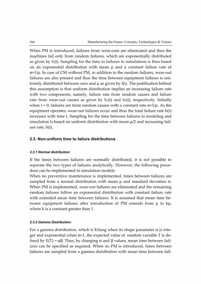
When PM is introduced, failures from wear-outs are eliminated and thus the

machines fail only from random failures, which are exponentially distributed

as given by f1(t). Sampling for the time to failures in simulations is then based

on an exponential distribution with mean µ and a constant failure rate of

α=1/µ. In case of CM without PM, in addition to the random failures, wear-out

failures are also present and thus the time between equipment failures is uni-

formly distributed between zero and µ as given by f(t). The justification behind

this assumption is that uniform distribution implies an increasing failure rate

with two components, namely, failure rate from random causes and failure

rate from wear-out causes as given by h1(t) and h2(t), respectively. Initially

when t = 0, failures are from random causes with a constant rate α=1/µ. As the

equipment operates, wear-out failures occur and thus the total failure rate h(t)

increases with time t. Sampling for the time between failures in modeling and

simulation is based on uniform distribution with mean µ/2 and increasing fail-

ure rate, h(t).

2.3. Non-uniform time to failure distributions

2.3.1 Normal distribution:

If the times between failures are normally distributed, it is not possible to

separate the two types of failures analytically. However, the following proce-

dure can be implemented in simulation models:

When no preventive maintenance is implemented, times between failures are

sampled from a normal distribution with mean µ and standard deviation σ.

When PM is implemented, wear-out failures are eliminated and the remaining

random failures follow an exponential distribution with constant failure rate

with extended mean time between failures. It is assumed that mean time be-

tween equipment failures after introduction of PM extends from µ to kµ,

where k is a constant greater than 1.

2.3.2 Gamma Distribution:

For a gamma distribution, which is Erlang when its shape parameter α is inte-

ger and exponential when α=1, the expected value of random variable T is de-

fined by E(T) = αβ. Thus, by changing α and β values, mean time between fail-

ures can be specified as required. When no PM is introduced, times between

failures are sampled from a gamma distribution with mean time between fail-


ures of αβ. If PM is introduced and wear-out failures are eliminated, times be-

tween failures are extended by a constant k. Therefore, sampling is made from

an exponential distribution with mean k(αβ).

2.3.3 Weibull Distribution:

For the Weibull distribution, α is a shape parameter and β is a scale parameter.

The expected value of time between failures, E(T)=MTBF=βΓ(1/α)/α, and its

variance is V(T)= β2[2Γ(2/α)-{Γ(1/α)}2/α]. For a given value of α,

β=α(MTBF)/Γ(1/α). When there is no PM, times between failures are sampled

from Weibull with parameters α and β in simulation models. When PM is in-

troduced, wear-out failures are eliminated and the random failures are sam-

pled in simulation from an exponential distribution with mean=k[βΓ(1/α)/α],

where α and β are the parameters of the Weibull distribution and k is a con-

stant greater than 1.

2.3.4 Triangular Distribution:

The triangular distribution is described by the parameters a, m, and b (i.e.,

minimum, mode, and maximum). Its mean is given by E(T)=(a+m+b)/3 and

variance by V(T) = (a2+m2+b2-ma-ab-mb)/18. Since the times between failures

can be any value starting from zero, we let a=0 and thus m=b/3 from the prop-

erty of a triangular distribution. Mean time between failures is

E(T)=(m+b)/3=[b+b/3]/3=4b/9=4m/3. If no PM is introduced, time between fail-

ures are sampled in simulation from a triangular distribution with parameters

a, m, b or 0, b/3, b. If PM is introduced, again wear-out failures are eliminated

and the random failures are sampled from an exponential distribution with an

extended mean of k[a+m+b]/3, where a, m, and b are parameters of the

triangular distribution that describe the time between failures. The multiplier k

is a constant greater than 1.

3. Analysis of the Effects of Maintenance Policies on FMS Availability

Equipment in FMS systems can be subject to corrective maintenance; correc-

tive maintenance combined with a preventive maintenance; and preventive

maintenance implemented at different opportunities. FMS operates with an in-

creasing failure rate due to random causes and wear-outs. The stream of mixed

failures during system operation is separated into two types: (i) random fail-

ures due to chance causes; (ii) time dependent failures due to equipment usage


and wear-outs. The effects of preventive maintenance policies (scheduled and

opportunistic), which are introduced to eliminate wear-out failures of an FMS,

can be investigated by analytical and simulation models. In particular, effects

of various maintenance policies on system performance can be investigated

under various time between failure distributions, including uniform, normal,

gamma, triangular, and Weibull failure time distributions, as well as different

repair and maintenance parameters.

3.1 Types of Maintenance Policies

In this section, five types maintenance policies, which resulted in six distinct

cases, and their effects on FMS availability are described.

i) No Maintenance Policy:

In this case, a fully reliable FMS with no failures and no maintenance is con-

sidered.

ii) Corrective Maintenance Policy (CM):

The FMS receives corrective maintenance only when equipment fails. Time be-

tween equipment failures can follow a certain type of distribution. In case of

uniform distribution, two different types of failures can be separated in model-

ing and analysis.

iii) Block-Based PM with CM Policy (BB):

In this case, the equipment is subject to preventive maintenance at the end of

each shift to eliminate the wear out failures during the shift. However, regard-

less of any CM operations between the two scheduled PMs, the PM operations

are always carried out as scheduled at the end of the shifts without affecting

the production schedule. This policy is evaluated under various time between

failure distributions. Figure 1 illustrates this maintenance process.

PM1 PM2 CM1 PM3 CM2 PM4

T T T

Figure 1. Illustration of PM operations under a block-based policy


iv) Age-Based PM with CM Policy (AB):

In this policy, preventive maintenance is scheduled at the end of a shift, but

the PM time changes as the equipment undergoes corrective maintenance.

Suppose that the time between PM operations is fixed as T hours and before

performing a particular PM operation the equipment fails. Then the CM opera-

tion is carried out and the next PM is rescheduled T hours from the time the

repair for the CM is completed. CM has eliminated the need for the next PM. If

the scheduled PM arrives before a failure occurs, PM is carried out as sched-

uled. Figure 2 illustrates this process.

PM1 PM2 CM1 PM3 PM3 (rescheduled)

T

Figure 2. Illustration of PM operations under age-based policy.

v) Opportunity-Triggered PM with CM Policy (OT):

In this policy, PM operations are carried out only when they are triggered by

failure. In other words, if a failure that requires CM occurs, it also triggers PM.

Thus, corrective maintenance as well as preventive maintenance is applied to

the machine together at the time of a failure. This is called triggered preventive

maintenance. Since the equipment is already stopped and some parts are al-

ready maintained for the CM, it is expected that the PM time would be re-

duced in this policy. We assign a certain percentage of reduction in the PM op-

eration. A 50% reduction was assumed reasonable in the analysis below.

vi) Conditional Opportunity-Triggered PM with CM Policy (CO): In this policy,

PM is performed on each machine at either scheduled times or when a speci-

fied opportunistic condition based on the occurrence of a CM arises. The main-

tenance management can define the specified condition. In our study, a spe-

cific condition is defined as follows: if a machine fails within the last quarter of

a shift, before the time of next PM, the next PM will be combined with CM for

this machine. In this case, PM scheduled at the end of the shift would be

skipped. On the other hand, if a machine failure occurs before the last quarter

of the shift, only CM is introduced and the PM is performed at the end of the

shift as it was scheduled. This means that the scheduled PM is performed only

for those machines that did not fail during the last quarter of the shift.


The maintenance policies described above are compared under similar operat-

ing conditions by using simulation models with analytical formulas incorpo-

rated into the model as described in section 2. The FMS production rate is first

determined under each policy. Then, using the production rate of a fully reli-

able FMS as a basis, an index, called Operational Availability Index (OAIi) of

the FMS under each policy i, is developed: OAIi=Pi/P1, where P1 = production

rate of the reliable FMS and Pi = production rate of the FMS operated under

maintenance policy i (i=2, 3, 4, 5, and 6). General formulation is described in

section 2 for five different times between failure distributions and their im-

plementation with respect to the maintenance policies. The following section

presents a maintenance simulation case example for an FMS system.

3.2 Simulation Modeling of FMS Maintenance Operations

In order to analyze the performance measures of FMS operations under differ-

ent maintenance policies, simulation models are developed for the fully reli-

able FMS and for each of the five maintenance related policies described

above. Simulation models are based on the SIMAN language (Pegden et al.,

1995). In order to experiment with different maintenance policies and to illus-

trates their effects on FMS performance, a case problem, as in figure 3 is con-

sidered. Table 1 shows the distance matrix for the FMS layout and Table 2

shows mixture of three different types of parts arriving on a cart, the sequence

of operations, and the processing times on each machine. An automated

guided vehicle (AGV) selects the parts and transports them to the machines

according to processing requirements and the sequence. Each part type is op-

erated on by a different sequence of machines. Completed parts are placed on

a pallet and moved out of the system. The speed of the AGV is set at 175

feet/minute. Parts arrive to the system on pallets containing 4 parts of type 1, 2

parts of type 2, and 2 parts of type 3 every 2 hours. This combination was fixed

in all simulation cases to eliminate the compounding effects of randomness in

arriving parts on the comparisons of different maintenance policies. The FMS

parameters are set based on values from an experimental system and previous

studies.

One simulation model was developed for each of the six cases as: i) A fully re-

liable FMS (denoted by FR); ii) FMS with corrective maintenance policy only

(CM); iii) FMS with block-based policy (BB); iv) FMS with age-based policy

(AB); v) FMS with opportunity-triggered maintenance policy (OP); and vi)

FMS with conditional opportunity-triggered maintenance policy (CO). Each


simulation experiment was carried out for the operation of the FMS over a pe-

riod of one month (20 working days or 9600 minutes). In the case of PM, it was

assumed that a PM time of 30 minutes (or 15 minutes when combined with

CM) is added to 480 minutes at the end of each shift. Twenty simulation repli-

cates are made and the average output rate during one month is determined.

The output rate is then used to determine the FMS operational availability in-

dex for each policy. The output rate is calculated as the average of the sum of

all parts of all types produced during the month. The fully reliable FMS dem-

onstrates maximum possible output (Pi) and is used as a base to compare other

maintenance policies with OAIi = Pi/P1.

Figure 3. A flexible manufacturing system

In Lathe Mill Grind Out

In - 100 75 100 40

Lathe - - 150 175 155

Mill - - - 50 90

Grind - - - - 115

Out - - - - -

Table 1. Distance matrix (in feet).

AGVLathe 2

GrinderMill

IN OUT

Lathe 1


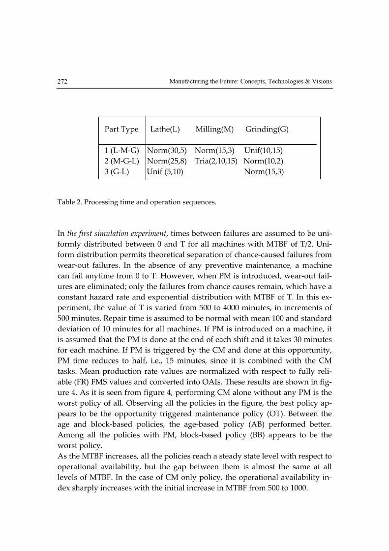
Part Type Lathe(L) Milling(M) Grinding(G)

1 (L-M-G) Norm(30,5) Norm(15,3) Unif(10,15)

2 (M-G-L) Norm(25,8) Tria(2,10,15) Norm(10,2)

3 (G-L) Unif (5,10) Norm(15,3)

Table 2. Processing time and operation sequences.

In the first simulation experiment, times between failures are assumed to be uni-

formly distributed between 0 and T for all machines with MTBF of T/2. Uni-

form distribution permits theoretical separation of chance-caused failures from

wear-out failures. In the absence of any preventive maintenance, a machine

can fail anytime from 0 to T. However, when PM is introduced, wear-out fail-

ures are eliminated; only the failures from chance causes remain, which have a

constant hazard rate and exponential distribution with MTBF of T. In this ex-

periment, the value of T is varied from 500 to 4000 minutes, in increments of

500 minutes. Repair time is assumed to be normal with mean 100 and standard

deviation of 10 minutes for all machines. If PM is introduced on a machine, it

is assumed that the PM is done at the end of each shift and it takes 30 minutes

for each machine. If PM is triggered by the CM and done at this opportunity,

PM time reduces to half, i.e., 15 minutes, since it is combined with the CM

tasks. Mean production rate values are normalized with respect to fully reli-

able (FR) FMS values and converted into OAIs. These results are shown in fig-

ure 4. As it is seen from figure 4, performing CM alone without any PM is the

worst policy of all. Observing all the policies in the figure, the best policy ap-

pears to be the opportunity triggered maintenance policy (OT). Between the

age and block-based policies, the age-based policy (AB) performed better.

Among all the policies with PM, block-based policy (BB) appears to be the

worst policy.

As the MTBF increases, all the policies reach a steady state level with respect to

operational availability, but the gap between them is almost the same at all

levels of MTBF. In the case of CM only policy, the operational availability in-

dex sharply increases with the initial increase in MTBF from 500 to 1000.


0.5

0.6

0.7

0.8

0.9

1.0

500 1000 1500 2000 2500 3000 3500 4000

MTBF

Ava

ilab

ility

In

de

x

Full Rel.

CM

BB

AB

OT

CO

Figure 4. Operational availability index under different maintenance policies.

As indicated above, when PM is introduced, time between failures become ex-

ponential regardless of the type of initial distribution. Experiments with dif-

ferent distributions show that all distributions give the same performance re-

sults under the last four maintenance policies, which include some form of

PM. However, FMS performance would differ under different failure distribu-

tions when a CM policy is implemented. This is investigated in the second ex-

periment, which compares the effects of various time to failure distributions,

including uniform, normal, gamma, Weibull, and triangular distributions, on

FMS performance under the CM policy only. All of the FMS parameters re-

lated to operation times, repair, and PM times were kept the same as given in

the first experiment. Only time to failure distributions and related parameters

were changed such that MTBF was varied between 500 and 4000.

In the case of the gamma distribution, E(T) = αβ. Thus, α = 250 and β= 2 re-

sulted in a MTBF of 500; α = 750 and β= 2 resulted in a MTBF=1500; α = 1250

and β= 2 resulted in a MTBF=2500; and α = 2000 and β= 2 resulted in a

MTBF=4000, which are the same values specified in the second experiment for

the normal distribution. For the Weibull distribution, which has MTBF=E(T)=

βΓ(1/α)/α, two the parameters α (shape parameter) and β (scale parameter)

have to be defined. For example, if MTBF=500 and α=2, then, 500=βΓ(1/α)/α


=βΓ(1/2)/2. Since Γ(1/2)=√π, β=1000/√π. Thus, for MTBF=500, β=564.2. Similarly,

for MTBF=1500, β=1692.2, for MTBF=2500, β=2820.95, and for MTBF=4000,

β=4513.5 are used. Triangular distribution parameters are also determined

similarly as follows: E(T) = (a+m+b)/3 and V(T)= (a2+m2+b2-ma-ab-mb)/18. Since

the times between failures can be any value starting from zero, we let a=0 and

m=b/3 from the property of triangular distribution. E(T)=

(m+b)/3=[b+b/3]/3=4b/9=4m/3. In order to determine values of the parameters,

we utilize these formula. For example, if MTBF =500, then 500=4b/9 and thus

b=4500/4 = 1125 and m=b/3=1500/4=375. Similarly, for MTBF=1500, b=3375 and

m=1125. For MTBF=2500, b=5625 and m=1875. For MTBF=4000, b=9000 and

m=3000. Table 3 presents a summary of the related parameters.

Distribution Parameters that result in

the specified MTBF

MTBF

α ぽ

500 250 2

1500 750 2

2500 1250 2

Gamma

4000 2000 2

500 2 564.2

1500 2 1692.2

2500 2 2820.95

Weibull

4000 2 4513.5

MTBF a b m

500 0 1125 375

1500 0 3375 1125

2500 0 5625 1875

Triangular

4000 0 9000 3000

Table 3. Parameters of the distributions used in simulation.

Comparisons of five distributions, uniform, normal, gamma, Weibull, and tri-

angular, with respect to CM are illustrated in figure 5, which plots the OAI

values normalized with respect to fully reliable system using production rates.

All of the distributions show the same trend of increasing OAI values, and

thus production rates, with respect to increasing MTBF values. As it seen in

figure 5, uniformly distributed time between failures resulted in significantly


different FMS availability index as compared the other four distributions. This

is because in a uniform distribution, which is structurally different from other

distributions, probability of failure is equally likely at all possible values that

the random variable can take, while in other distributions probability concen-

tration is around the central value. The FMS performance was almost the same

under the other four distributions investigated. This indicates that the type of

distribution has no critical effects on FMS performance under CM policy if the

distribution shapes are relatively similar.

0,5

0,6

0,7

0,8

0,9

1,0

500 1500 2500 4000MTBF

Availa

bili

ty Index

Full Rel.

Uniform

Normal

Gamma

Weibull

Triangular

Figure 5. FMS OAI under various time to failure distributions and CM policy

The results of the analysis show that maintenance of any form has significant

effect on the availability of the FMS as measured by its output rate. However,

the type of maintenance applied is important and should be carefully studied

before implementation. In the particular example studied, the best policy in all

cases was the opportunity-triggered maintenance policy and the worst policy

was the corrective maintenance policy. The amount of increase in system

availability depends on the maintenance policy applied and the specific case

studied. Implementation of any maintenance policy must also be justified by a

detailed cost analysis.


The results presented in this chapter show a comparative analysis of specified

maintenance policies with respect to operational availability measured by out-

put rate. Future studies can be carried out on the cost aspects of various poli-

cies. The best cost saving policy can be determined depending on the specified

parameters related to the repair costs and the preventive maintenance costs. In

order to do cost related studies, realistic cost data must be collected from in-

dustry. The same models developed and procedures outlined in this paper can

be used with cost data. Other possible maintenance policies must be studied

and compared to those presented in this study. Combinations of several poli-

cies are also possible within the same FMS. For example, while a set of equip-

ment is maintained by one policy, another set could be maintained by a differ-

ent policy. These aspects of the problem may also be investigated by the

models presented.

4. Analysis of the Effects of Maintenance Policies on Serial Lines

Multi-stage discrete part manufacturing systems are usually designed along a

flow line with automated equipment and mechanized material flow between

the stations to transfer work pieces from one station to the next automatically.

CM and PM operations on serial lines can cause significant production losses,

particularly if the production stages are rigidly linked. In-process inventories

or buffer storages are introduced to decouple the rigidly-linked machinery and

to localize the losses caused by equipment stoppages. Buffer storages help to

smooth out the effect of variation in process times between successive sta-

tions and to reduce the effects of CM and PM in one station over the adja-

cent stations. While large buffer capacities between stages result in excessive

inventories and costs, small buffer capacities result in production losses due to

unexpected and planned stoppages and delays. One of the major problems as-

sociated with the design and operation of a serial production system is the de-

termination of the effects of maintenance activities coupled with certain buffer

capacities between the stations. Reliability and productivity calculations of

multi-stage lines with maintenance operations and intermediate storage units

can be quite complex. Particularly, closed form solutions are not possible when

different types of maintenance operations are implemented on the machines.

Production line systems can take a variety of structures depending on the op-

erational characteristics. Operation times can be stochastic or deterministic;

stations can be reliable or unreliable; buffer capacities can be finite or infinite;


production line can be balanced or unbalanced; and material flow can be con-

sidered as discrete or continuous. Depending on the type of line considered

and the assumptions made, complexity of the models vary. The objective in

modeling these systems is to determine line throughput rate and machine

utilizations as a function of equipment failures, maintenance policies, and

buffer capacities,. Optimum buffer allocation results in maximum throughput

rate. Algorithms and models are developed for buffer allocation on reliable

and unreliable production lines for limited size problems. While closed form

analytical models or approximations are restricted by several assumptions,

models that can be coupled with numerical evaluation or computer simulation

are more flexible and allow realistic modeling.

In this chapter we present a discrete mathematical model, which is incorpo-

rated into a generalized iterative simulation procedure to determine the pro-

duction output rate of a multi-stage serial production line operating under dif-

ferent conditions, including random failures with corrective and preventive

maintenance operations, and limited buffer capacities. The basic principal of

the discrete mathematical model is to determine the total time a part n spends

on a machine i, the time instant at which part n is completed on machine i, and

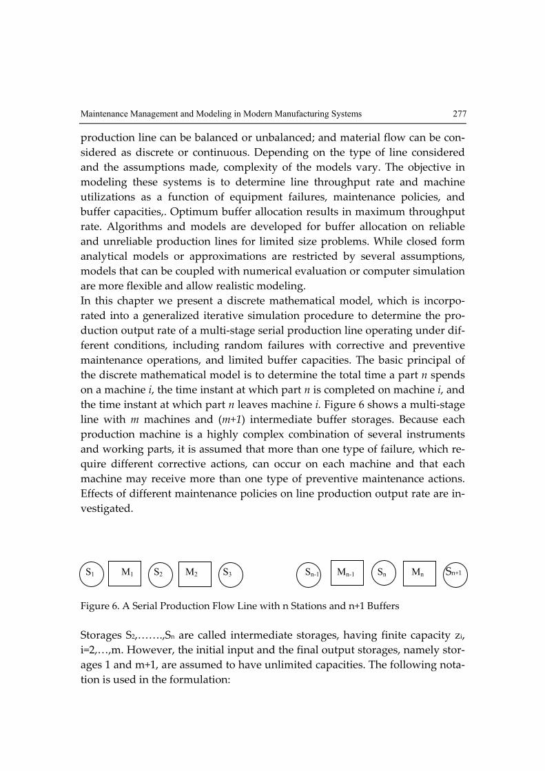
the time instant at which part n leaves machine i. Figure 6 shows a multi-stage

line with m machines and (m+1) intermediate buffer storages. Because each

production machine is a highly complex combination of several instruments

and working parts, it is assumed that more than one type of failure, which re-

quire different corrective actions, can occur on each machine and that each

machine may receive more than one type of preventive maintenance actions.

Effects of different maintenance policies on line production output rate are in-

vestigated.

S1 M1 S2 M2 S3 Sn-1 Mn-1 Sn Mn Sn+1

Figure 6. A Serial Production Flow Line with n Stations and n+1 Buffers

Storages S2,…….,Sn are called intermediate storages, having finite capacity zi,

i=2,…,m. However, the initial input and the final output storages, namely stor-

ages 1 and m+1, are assumed to have unlimited capacities. The following nota-

tion is used in the formulation:


- Rin= Total duration of time that nth part stays on the ith machine not consi-

dering imposed stoppages due to maintenances or failures; i=1,2,…..,m.

- m = Number of machines on the line.

- Pijn = Duration of preventive maintenance of jth type on the ith machine after

machining of nth part is completed; j=1,2,…….,npi

- npi = Number of preventive maintenance types performed on machine i

- tin = Machining time for part n on machine i. This time can be assumed to

be independent of n in the simulation program.

- rijn = Repair time required by ith machine for correction of jth type of failu-

res which occur during the machining of nth part; j=1,2,…..,nfi

- nfi = Number of failure types which occur on machine i.

- Cin = Instant of time at which machining of nth part is completed on ith ma-

chine.

- Din = Instant of time at which nth part departs from the ith machine.

- D0n = Instant of time at which nth part enters the 1st machine.

- Win = Instant of time at which ith machine is ready to process nth parts.

A part stays on a machine for two reasons: Either it is being machined or the

machine is under corrective maintenance because a breakdown has occurred

during machining of that part. Rin, which is the residence time of the nth part on

the ith machine, without considering imposed stoppages for corrective mainte-

nance, is given as follows:

∑=

+=inf

j

ijninin rtR1

(14)

The duration of total preventive maintenance, Pin, performed on the ith machine

after completing the nth part, is equal to the total duration of all types of pre-

ventive maintenances, Pijn, that must be started after completion of nth part as:

∑=

=inp

j

ijnin PP1

(15)

Each buffer Bi is assumed to have a finite capacity zi, i=2,3,……,m. The discrete

mathematical model of serial line consists of calculating part completion times,

Cin, and part departure times, Din, in an iterative fashion.


4.1 Determination of Part Completion Times

Machining of part n cannot be started on machine i until the previous part, n-1,

leaves machine i and until all the required maintenances, if necessary, are per-

formed on machine i. Therefore the time instant at which ith machine is ready

to begin the nth part, denoted by Win, is given by the following relation:

Win = max[Di,n-1, Ci,n-1+Pi,n-1] (16)

If Di-1,n<Win, then the nth part must wait in storage buffer Si, since it has left ma-

chine i-1 before machine i is ready to accept it. Therefore, machining of part n

on machine i will start at instant Win. If however, Di-1,n≥Win, then machining of

the nth part on the ith machine can start immediately after Di-1,n. Considering

both cases above, starting time of the nth part to be machined on the ith machine

is:

max[Di-1,n, Di,n-1, Ci,n-1+Pi,n-1] (17)

Since the nth part will stay on machine i for a period of Rin time units, its ma-

chining will be completed by time instant Cin given by:

Cin= max[Di-1,n, Di,n-1, Ci,n-1+Pi,n-1] + Rin (18)

Where

i=2,3,……,m and C1n= max[D1,n-1, C1,n-1+P1,n-1] + R1n (19)

Then,

D0n< max[D1,n-1, C1,n-1+P1,n-1], (20)

assuming there are always parts available in front of machine 1.


4.2 Determination of Part Departure Times

The time instant at which nth part leaves the ith machine, Din, is found by con-

sidering two cases.

Let k = n– zi+1–1. Then, in the first case:

],max[ ,1,1,1, kikikini PCDC +++ +< (21)

which indicates that the nth part has been completed on the ith machine before

machining of the (n- zi+1)th part has started on the (i+1)th machine. Since storage

i+1, which is between machine i and i+1 and has capacity zi+1, is full and ma-

chine i has completed the nth part, the nth part may leave the ith machine only at

the instant of time at which the (n–zi+1)th part of the (i+1)th machine has started

machining. Therefore,

],max[ ,1,1,1, kikikini PCDD +++ += (22)

In the second case:

],max[ ,1,1,1, kikikini PCDC +++ +> (23)

which indicates that, at the instant Ci,n there are free spaces in buffer Si+1 and

therefore part n can leave machine i immediately after it is completed; that is,

Di,n = Ci,,n holds under this case. Considering both cases above, we have the fol-

lowing relations for Di,,n:

1 if 1,, +≤= +inini znCD , (24)

],,max[ ,1,1,1,, kikikinini PCDCD +++ += (25)

if n > zi+1+1; i =1, 2, 3,……, m–1 and k = n – zi+1–1.

Since the last stage has infinite space to index its completed parts,

Dm,,n = Cm,,n (26)


The simulation model, which is based on discrete mathematical model, can it-

eratively calculate Ci,n and Di,n from which several line performance measures

can be computed. Performance measures estimated by the above iterative

computational procedures are: (i) Average number of parts completed by the

line during a simulation period, Tsim; (ii) Average number of parts completed

by each machine during the time, Tsim; (iii) Percentage of time for which each

machine is up and down; (iv) Imposed, inherent and total loss factors for each

machine; (v) Productivity improvement procedures.

In addition to the variables described for the discrete model in previous sec-

tion, the simulation model can allow several distributions, including: exponen-

tial, uniform, Weibull, normal, log normal, Erlang, gamma, beta distributions

and constant values to describe failure and repair times. After the production

line related parameters and all data are entered into the simulator and neces-

sary initializations are carried out by the program, iterative analysis of the

production line is performed through the discrete mathematical model. The it-

erative analysis provides one simulation realization of the production line for a

specified period of simulation time (Tsim). It basically calculates iteratively the

time instant at which each part enters a machine, duration of its stay, and the

time it leaves the machine. This is continued until, for example one shift is

completed. The results of each iterative simulation are then utilized with statis-

tical tests to determine if the specified conditions are met to stop the number of

simulation iterations. If the conditions are not met, simulation iterations are

continued with further runs. For each simulation realization, calculations of

Ri,n, Ci,n, and Di,n are performed based on the need for repair or preventive

maintenance operations as the parts flow through the system.

4.3 Statistical Analysis and Determination of Need for More Realizations

Reliable results cannot always be obtained from a single simulation realiza-

tion. Therefore, additional runs have to be performed and the results tested

statistically until the error in the line production rate is less than an epsilon

value with a probability, both of which are predefined. This is accomplished as

follows:

Let Ni = number of parts produced by the production line during the ith simula-

tion run. Ni is a random variable which approaches normal distribution as

t→∞; that is, as the simulation time increases for ach realization, the sample

random variable Ni approaches to an asymptotic normal distribution. The


mean value of Ni, N , and its variance V(N) are given by ( )∑=

=n

i

i nNN1

and

∑=

−−=n

i

i nNNNV1

2 )1/()()( , where n represents the number of runs. The average line

production rate, Q , which is the average output rate per unit of time, is given

by simTNQ /= where Tsim is the simulation time for each realization, given in

minutes. The quantity Q is the average line production rate in parts/minute.

The variance of Q , )(QV , is determined by 22 )(/)(/)()/()( simsimsim TnNVTNVTNVQV === , since nNVNV /)()( = . The standard de-

viation of the average production rate, Q , is )(QV and the ratio of its stan-

dard deviation to its mean is expressed as by:

NnNVnNNVTNnTNVQQV simsim /]/)([]/[])([]//[]/)([/)( === . Since the number

of parts Ni produced by the production line during a simulation period Tsim

approaches the normal distribution, one can determine a confidence interval

forN and Q using the normal distribution. ∫∞−

−=⎥⎥⎦⎤

⎢⎢⎣⎡

<− x

Z dzexNV

NN 22

2

1

)(Pr

π. The

value of N is contained, with probability 1 – α, in the interval given by

α−=⎥⎥⎦⎤

⎢⎢⎣⎡

<−

<− αα 1)(

Pr 22 ZNV

NNZ

. Since the mean output rate, Q , is given by simTNQ = ,

one can conclude that Q is normally distributed, as are N and N . Therefore, a

confidence interval for the actual mean output rate Q would be given by

α−=⎥⎥⎦⎤

⎢⎢⎣⎡

<−

<− αα 1)(

Pr 22 ZQV

QQZ

or by ( )[ ] ααα −=+<<− 1)(1))(1(Pr 22 QQVZQQQQVZQ

α−=⎥⎥⎦⎤

⎢⎢⎣⎡

+<<− αα1

)(1

)(1Pr

22

Q

QVZ

Q

Q

Q

QVZ (27)

Our aim is to have an estimated output rate, Q , as close to the actual mean

output rate Q as possible. To achieve this, QQVZ )(2α is minimized by ob-

taining more runs. As this value gets closer to 0, Q →Q with probability 1 – α.

An ε value is entered by the user; the simulation program calculates

QQVZ )(2α after each iteration; compares this quantity with ε and termi-

nates the program if it is less than ε. If it is not less than ε after a maximum

number of iterations entered by the user, the program is still terminated to

avoid excessive computation time. However, the results may not be as reliable.


4.4 Productivity Improvement Procedure

Operational characteristics, such as machining or operation times, equipment

failures, corrective and preventive maintenance activities, and intermediate

buffer capacities have significant effects on the production line efficiency. As-

sessment of the operational efficiency of an automated manufacturing line

with storage units by computer simulation permits one to determine various

possible parameters and dependent variables which have the most significant

effects on productivity. Estimation indices are obtained for such variables as

the total, inherent, and imposed relative time losses due to failures and stop-

pages for each machine. These variables are obtained by employing failure and

repair times and nominal and relative production rates for each machine.

These terms are defined as follows:

)(/60)( itiQn = is the normal productivity of machine i, where t(i) is the cycle

time for machine i; simr TNiQ /60)( = is the relative productivity of machine i;

)(/)(1)(loss iQiQiK nr−= is the total loss factor of machine i;

)]()(/[)(1)(inh itititiK frr +−= is inherent loss factor of machine i; and

)()()( inhlossimp iKiKiK −= = )]()(/[)()(/)(1 itititiQiQ frrnr +−− is the imposed loss

factor for machine i, i = 1, 2, ….., m. The terms )(it f and )(itr are mean times to

failure and repairs, respectively of machine i. After determining these loss fac-

tors, the program can compare total loss factors for all machines. The machine

or stage which has the highest total loss factor is then chosen for improvement.

This machine’s imposed and inherent losses are compared.

The following two suggestions are made.

(i) If Kimp(i)>Kinh(i), it is suggested that the capacity of storages immediately

preceding and succeeding machine i with highest total loss factor should be

increased. Reliability and productivity of machine i–1 and machine i+1 should

also be increased.

(ii) If Kinh(i)>Kimp(i), stoppages are mainly caused by inherent failures, that is

breakdowns. Therefore, the reliability of machine i should be increased by PM

or its mean repair time should be decreased in order to gain improvement in

total productivity. After the changes are made, simulation should be repeated

to see the effects of the proposed changes in the line design.


4.5 Case Problem and Simulation Results

In order to illustrate the model developed above and to demonstrate the ef-

fects of maintenance operations on the productivity of serial production lines

with intermediate buffers, two case problems are considered as follows.

Case problem 1: A balanced serial production line with 5 stations is considered.

Operation times are 1.25 minutes on all stations; Number of failure types on

each equipment is 2 failures; Distributions of time to failure and related pa-

rameters are Uniform (0, 120) and Uniform (0, 180) with means of 60 and 90

minutes respectively; Distributions of repair times and related parameters are

Normal (5, 1) and Normal (7, 1.5); Buffer storage capacities between stations

are varied from 1 to 10. When a preventive maintenance is implemented on the

line, wear out failures are eliminated and only random failures, with constant

failure rates, remain. Time between failures extend from uniform to exponen-

tial as explained in section 2.4.

Average line output rate (parts/min) = 0.674104

Standard deviation of line output rate = 0.0031194163

Machine

Number

Total

Parts Pro-

duced

Relative

Production

Rate

Nominal

Production

Rate

Imposed

Loss Fac-

tor

Inherent

Loss Fac-

tor

1 8102.250 40.515 48.000 0.081 0.075

2 8099.750 40.508 48.000 0.083 0.073

3 8096.250 40.484 48.000 0.080 0.077

4 8089.750 40.456 48.000 0.084 0.074

5 8089.250 40.448 48.000 0.084 0.073

Machine 5 has the maximum total loss factor.

Down time is mainly imposed: increase the capacity of storage adjacent to

this machine, also increase reliability by PM; increase productivity of adjacent

machines; reduce the CM times and try simulation again.

Maximum iteration is reached at 75.

Table 4. Iterative Simulation Output Results for Production Line Case 1


Two types of PM with intervals of 120 minutes and 180 minutes (correspond-

ing to 96 parts and 144 parts) are assumed to be implemented to eliminate

wear out failures; PM times are 2.5 and 3.5 time units. Time to failure distribu-

tions change to exponential with mean time to failures of 120 and 180 minutes.

Distributions of repair times and related parameters are Normal (5, 1) and

Normal (7, 1.5). Buffer storage capacities are again varied between 1 and 10

units. Parameters related to statistical tests were set as follows: ぼ=0.05;

Zぼ/2=1.96; ε=0.001, maximum number of iterations=200; and production simula-

tion time was 12,000 minutes. Table 4 shows one output example for the bal-

anced line case under CM&PM policy when maximum buffer capacity of 10

units are allowed between the stations. Average line output rate obtained is

0.674104 parts/minute. Station production rates, loss factors, and suggestion

for improvements are also shown in the table. Related results obtained for all

other cases of buffer sizes are summarized in Figure 7.

The effects of CM only policy and the policy of implementing PM with CM

(CM and PM), under different buffer capacities are illustrated in the figure. An

increase in production rate is achieved due to PM implementation for all cases

of buffer capacities. The increase in production rate levels off as the buffer ca-

pacity is increased.

Case Problem 2: In addition to the balanced line case as shown in figure 7, three

unbalanced cases, with a bottleneck station at the beginning, at the middle,

and at the end of the line, are considered. Figure 8 shows the results for three

unbalanced line cases under CM as well as CM with PM policies. It is assumed

that a bottleneck station with operation time of 1.50 minutes is located at the

beginning (designated as Bottleneck at Start=BS in figure 8), in the middle (Bot-

tleneck in Middle=BM), or at the end of the line (Bottleneck at End=BE). As it is

seen in the figure, all CM & PM cases result in higher production rate than CM

only cases. Figure 8 also shows that when the bottleneck station is in the mid-

dle of the line, production rate is less than the cases of bottleneck being at the

beginning or at the end of the line. These two last cases result in almost equal

production rates as can be seen in the figure. The discrete model and the re-

lated program can also be used to perform an exhaustive search to find the op-

timum allocation of total fixed buffer capacity to the stages to maximize the

line production rate.


0.50

0.54

0.58

0.62

0.66

0.70

1 2 3 4 5 6 7 8 9 10Buffer Capacity

Pro

du

cti

on

Rate

CM Only CM and PM

Figure 7. Comparison of CM policy with CM & PM policy for the balanced line

0.46

0.50

0.54

0.58

1 2 3 4 5 6 7 8 9 10

Buffer Capacity

Pro

du

cti

on

Rate

CM-BS CM-BM CM-BE

CM & PM-BS CM & PM-BM CM & PM-BE

Figure 8. Comparison of CM policy with CM & PM policy for unbalanced line


5. Concluding Remarks

This chapter has presented some basic concepts in maintenance modeling for

production systems. Mathematical models are developed for separation of dif-

ferent types of failure rates to evaluate effects of maintenance on equipment

productivity. The models were first applied to a FMS through simulation and

the results were discussed. It is found that PM of any type results in higher

productivity than CM only. However, depending on the type of system con-

sidered, some PM policies perform better than others. The best policy must be

determined by the analysis of the given system using the tools presented.

In order to analyze the effects of maintenance on the performance of serial

production lines, a discrete mathematical model and an iterative computer

simulation are developed for multi-stage production lines. The model allows

several types of failures and maintenances to be incorporated into the analysis.

Based on the discrete model, simulation approach incorporates a three-stage

procedure which allows the user to enter a set of data describing the system

under study, simulates the system until selected statistical criteria are satisfied

and obtains output results. Specific recommendations for productivity increase

can be applied until a satisfactory production output is achieved. The model is

applied to the cases of balanced and unbalanced lines and the effects of PM are

investigated. When PM was implemented in addition to CM, line productivity

was significantly increased. The discrete model and the iterative simulation

procedure proved to be very useful in estimating the production line produc-

tivity for complex realistic production systems. It allows the line designer or

operation managers to evaluate the effects of storage-unit capacity and re-

pair/maintenance policies on line productivity. As a future study, the sug-

gested iterative model can be incorporated into an interactive visual computer

software to be effectively utilized by design engineers and operation manag-

ers.

Acknowledgement

This chapter was prepared based on a research that was supported by Kuwait

University Research Administration under the grant number EI02/03.


6. References

Albino, V., Carella, G., and Okogbaa, O. G. (1992). Maintenance Policies in

Just-in-time Manufacturing Lines. International Journal of Production Re-

search, Vol. 30, No. 2, 369-382.

Al-Najjar, B., Alsyouf, I. (2003). Selecting the Most Efficient Maintenance Ap-

proach Using Fuzzy Multiple Criteria Decision Making. International

Journal of Production Economics, Vol. 84, No. 1, 85-100.

Ben-Daya, M. and Makhdoum, M. (1998). Integrated Production and Quality

Model Under Various Preventive Maintenance Policies. Journal of the Op-

erational Research Society, Vol. 49, 840-853.

Boukas, K. and Haurie, A. (1990). Manufacturing Flow Control and Preventive

Maintenance: A Stochastic Control Approach. IEEE Transactions on Auto-

matic Control, Vol. 35, No. 9, 1204-1031

Castro, H. F. D. and Cavalce, K. L.(2006). Maintenance Resources Optimization

Applied to a Manufacturing System. Reliability Engineering and System

Safety, Vol. 91, 413-420.

Chan, F. T. S., Lau, H. C. R., Ip, R. W. L., Chan, H. K., and Kong, S. (2005).

Implementation of Total Productive Maintenance: A Case Study. Interna-

tional Journal of Production Economics, Vol. 95, No. 1, 71-94.

Cho, I. D. and Parlar, M. (1991). A Survey of Maintenance Models for Multi-

unit Systems. European Journal of Operational Research, Vol. 51, 1-23.

Creehan, K. D. (2005). Establishing Optimal Maintenance Practices in a Tradi-

tional Manufacturing Environment. Journal of the Chinese Institute of Indus-

trial Engineers, Vol. 22, No. 1, 11-18.

Dekker, R. and Smeitnik, E. (1994). Preventive Maintenance at Opportunities

of Restricted Duration. Naval Research Logistics, Vol. 41, 335-353.

Dekker, R.(1996). Applications of Maintenance Optimization Models: A Re-

view and Analysis. Reliability Engineering and System Safety. Vol. 51, 229-

240.

Gupta, Y. P., Somers, T. M., and Grau, L. (1998). Modeling the Interrelation-

ship Between Downtimes and Uptimes of CNC Machines. European Jour-

nal of Operational Research, Vol. 37, 254-271.

Kennedy, W. J. (1987). Issues in the Maintenance of Flexible Manufacturing

Systems. Maintenance Management International, Vol. 7, 43-52

Kyriakidis, E. G. and Dimitrakos, T. D. (2006). Optimal Preventive Mainte-

nance of a Production System with an Intermediate Buffer. European Jour-

nal of Operational Research, Vol. 168, 86-99.


Levitin, G. and Meizin, L. (2001). Structure optimization for continuous pro-

duction systems with buffers under reliability constraints. International

Journal of Production Economics, Vol. 70, 77-87.

Lin, C., Madu, N.C., and Kuei C. (1994). A Closed Queuing Maintenance Net-

work for a Flexible Manufacturing System. Microelectronics Reliability, Vol.

34, No. 11, 1733-1744.

McKone, K. and Wiess, E. (1998). TPM: Planned and Autonomous Mainte-

nance: Bridging the Gap Between Practice and Research. Production an

Operations Management, Vol. 7, No. 4, 335-351.

Mobley, R. K. (1990). An Introduction to Predictive Maintenance. Van Nostrand

Reinhold. New York.

Papadopoulos, H. T. and Heavey, C. (1996). Queuing Theory in Manufacturing

Systems Analysis and Design: A Classification of Models for Production

and Transfer Lines. European J. of Operational Research, Vol. 92, 1-27.

Pegden, C.D., Shannon, R.E., and Sadowski, R. P. (1995). Introduction to Simula-

tion Using SIMAN, 2ndedition, McGraw Hill, New York.

Pintelon, L. M. and Gelders, L. F. (1992). Maintenance Management Decision

Making. European Journal of Operational Research, Vol. 58, 301-317.

Savsar, M. and Biles, W. E. (1984). Two-Stage Production Lines with Single

Repair Crew. International J. of Production Res., Vol. 22, No.3, 499-514.

Savsar, M. (1997a). Modeling and Analysis of a Flexible Manufacturing Cell.

Proceedings of the 22nd International Conference on Computers and Industrial

Engineering, December 20-22, Cairo, Egypt, pp. 184-187.

Savsar, M. (1997b) Simulation Analysis of Maintenance Policies in Just-In-Time

Production Systems. International Journal of Operations & Production Man-

agement, Vol. 17, No. 3, 256-266

Savsar, M. (2000). Reliability Analysis of a Flexible Manufacturing Cell. Reli-

ability Engineering and System Safety, Vol. 67, 147-152

Savsar, M. and Youssef, A. S. (2004). An Integrated Simulation-Neural Net-

work Meta Model Application in Designing Production Flow Lines.

WSEAS Transactions on Electronics, Vol. 2, No. 1, 366-371.

Savsar, M. (2005a). Performance Analysis of FMS Operating Under Different

Failure Rates and Maintenance Policies. The International Journal of Flexible

Manufacturing Systems, Vol. 16, 229-249.

Savsar, M. (2005b) Buffer Allocation in Serial Production Lines with Preven-

tiveand Corrective Maintenance Operations. Proceedings of Tehran Interna-


tional Congress on Manufacturing Engineering (TIMCE’2005), December 12-

15, 2005, Tehran, Iran.

Savsar, M. (2006). Effects of Maintenance Policies on the Productivity of Flexi-

ble Manufacturing Cells. Omega, Vol. 34, 274-282.

Sheu, C. and Krajewski, L.J. (1994). A Decision Model for Corrective Mainte-

nance Management. International Journal of Production Research, Vol. 32,

No. 6, 1365-1382.

Sun, Y. (1994). Simulation for Maintenance of an FMS: An Integrated System of

Maintenance and Decision-Making. International Journal of Advance Manu-

facturing Technology, Vol. 9, 35-39.

Valdez-Flores, C. and Feldman, R.M. (1989). A Survey of Preventive Mainte-

nance Models for Stochastically Deteriorating Single-Unit Systems. Naval

Research. Logistics, Vol. 36, 419-446.

Vatn, J., Hokstad, P., and Bodsberg, L. (1996). An Overall Model for Mainte-

nance Optimization. Reliability Engineering and System Safety, Vol. 51, 241-

257

Vineyard M. L. and Meredith J. R. (1992). Effect of Maintenance Policies on

FMS Failures. Int. J. of Prod. Research, Vol. 30, No. 11, 2647-2657.

Vouros, G. A., Vidalis, M. I., Papadopoulos, H. T. (2000). A Heuristic Algo-

rithm for Buffer Allocation in Unreliable Production Lines. International

Journal of Quantitative Methods, Vol. 6, No. 1, 23-43.

Waeyenbergh, G. and Pintelon, L. (2004). Maintenance Concept Development:

A Case Study. International J. of Production Economics, Vol. 89,395-405.

Manufacturing the FutureEdited by Vedran Kordic, Aleksandar Lazinica and Munir Merdan

ISBN 3-86611-198-3Hard cover, 908 pagesPublisher Pro Literatur Verlag, Germany / ARS, Austria Published online 01, July, 2006Published in print edition July, 2006

InTech EuropeUniversity Campus STeP Ri Slavka Krautzeka 83/A 51000 Rijeka, Croatia Phone: +385 (51) 770 447 Fax: +385 (51) 686 166www.intechopen.com

InTech ChinaUnit 405, Office Block, Hotel Equatorial Shanghai No.65, Yan An Road (West), Shanghai, 200040, China

Phone: +86-21-62489820 Fax: +86-21-62489821

The primary goal of this book is to cover the state-of-the-art development and future directions in modernmanufacturing systems. This interdisciplinary and comprehensive volume, consisting of 30 chapters, covers asurvey of trends in distributed manufacturing, modern manufacturing equipment, product design process,rapid prototyping, quality assurance, from technological and organisational point of view and aspects of supplychain management.

How to referenceIn order to correctly reference this scholarly work, feel free to copy and paste the following:

Mehmet Savsar (2006). Maintenance Management and Modeling in Modern Manufacturing Systems,Manufacturing the Future, Vedran Kordic, Aleksandar Lazinica and Munir Merdan (Ed.), ISBN: 3-86611-198-3,InTech, Available from:http://www.intechopen.com/books/manufacturing_the_future/maintenance_management_and_modeling_in_modern_manufacturing_systems

© 2006 The Author(s). Licensee IntechOpen. This chapter is distributed under the terms of theCreative Commons Attribution-NonCommercial-ShareAlike-3.0 License, which permits use,distribution and reproduction for non-commercial purposes, provided the original is properly citedand derivative works building on this content are distributed under the same license.

https://creativecommons.org/licenses/by-nc-sa/3.0/

Date post:	21-May-2020
Category:	Documents
Upload:	others
View:	3 times
Download:	0 times

Maintenance Management and Modeling in Modern ... · Maintenance Management and Modeling in Modern...

Documents