51
@ProfAndyField Making Statistics Easy by Getting your PENIS out in the Classroom Professor Andy Field
| Date post: | 16-Mar-2018 |
| Category: |
Documents |
| Upload: | hoangkhuong |
| View: | 217 times |
| Download: | 1 times |

@ProfAndyField
Making Statistics Easy by Getting your PENIS out in
the Classroom
Professor Andy Field

@ProfAndyField
Outline
! Part 1: ! Why should students love statistics?
! Part 2: ! Why do students hate statistics?
! Part 3: ! Can we make them like statistics more by exposing
them to my PENIS?

@ProfAndyField
A Scientist (Arguably)
Intelligent Laypeople

@ProfAndyField
Statistics is a life skill ! Utts (2003) some core skills:
1. When causal relationships can and cannot be inferred. 2. The difference between statistical significance and
practical importance. 3. The difference between finding ‘no effect' and finding
no statistically significant effect. 4. Sources of bias in surveys and experiments, such as poor
wording of questions, volunteer response, and socially desirable answers.
5. Understanding that variability is natural, and that ‘normal’ is not the same as ‘average’ (e.g., child development).
! Gordon (2004) ! 7% of Psychology students think statistics is generally
useful ! 16% thought it was useful for psychologyJ

@ProfAndyField
How the contraceptive pill works

@ProfAndyField
The Daily Mail Said... ! “Women may suffer a permanent decline in sex drive after
taking the contraceptive pill, researchers have said.”
! “A number of sexual dysfunction effects are associated with the Pill, including dulled libido ... Until now it has always been assumed that these are reversible, and cease to be a problem as soon as a woman comes off the Pill. But new research suggests that the effect on libido might be long lasting or even permanent.”
! “A team of American researchers ... studied 125 young women attending a sexual dysfunction clinic. Sixty two were taking oral contraceptives, 40 had previously taken them, and 23 had never been on the Pill.”
! “The scientists measured levels of SHBG in the women every three months for a year, and found they were seven times higher in users of the Pill than in women who had never taken them.”
! “Levels declined in women who had stopped taking the Pill, but remained three to four times higher than they were in those with no history of using oral contraceptives.”
@ProfAndyField
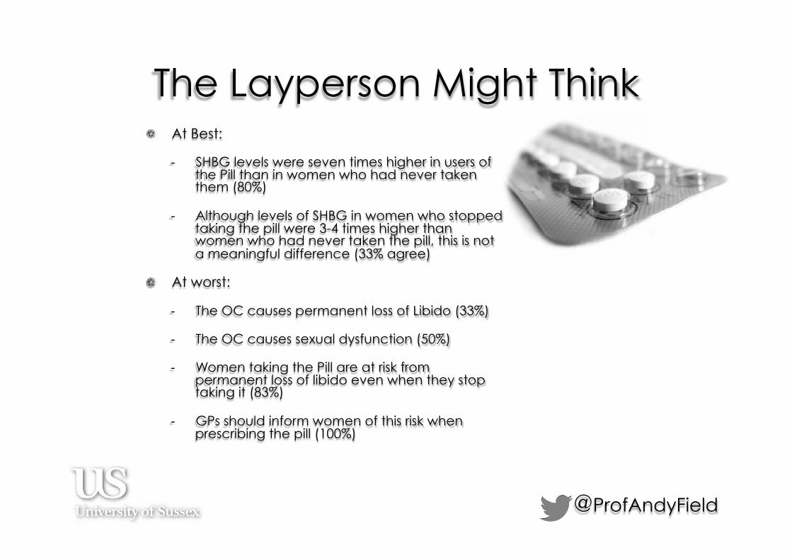
The Layperson Might Think ! At Best:
- SHBG levels were seven times higher in users of the Pill than in women who had never taken them (80%)
- Although levels of SHBG in women who stopped taking the pill were 3-4 times higher than women who had never taken the pill, this is not a meaningful difference (33% agree)
! At worst:
- The OC causes permanent loss of Libido (33%)
- The OC causes sexual dysfunction (50%)
- Women taking the Pill are at risk from permanent loss of libido even when they stop taking it (83%)
- GPs should inform women of this risk when prescribing the pill (100%)

Panzer et al.
0
50
100
150
200
250
Never Taken Pill
On Pill Stopped Taking Pill
Lib
ido
(SH
GB)
Group
Baseline
>120 Days
Normal
Lower

Panzer et al.
42 35
209
80
0
50
100
150
200
250
Baseline > 120 Days
Lib
ido
(SH
GB)
Group
Never Taken Pill
Stopped Taking Pill
Normal
Lower

@ProfAndyField
The Psychologist Copy Editor ...
! “Women with sexual dysfunction may suffer a permanent (well, up to 3-6 months or a year) decline in levels of SHBG after taking the contraceptive pill, researchers have said.”
! “A number of sexual dysfunction effects are associated with the Pill, including dulled libido ... Until now it has always been assumed that these are reversible and in the current research SHBG did actually decline a lot after coming off of the Pill, and cease to be a problem as soon as a woman comes off the Pill. But new research suggests that the effect on SHBG might be long lasting or even permanent even though we only have data over, on average 3-6 months.”
! “The scientists measured levels of SHBG in the women every three months for a year (well, some of them, the average was 3-6 months), and found they were seven (in a parallel universe where 7 = 5) times higher (at baseline, not after they’d come off the pill) in users of the Pill than in women who had never taken them.”
! “Levels declined in women who had stopped taking the Pill, but remained three to four times higher (in another parallel universe where 3 to 4 means 2.29) than they were in those with no history of using oral contraceptives. However, women in the discontinued group were followed up on average for 73 days less than never users (or 38 days less for the long term follow up group).”
! Subjective libido was never compared at follow-up in discontinued users and never-users, so we don’t really know a lot about libido one way or another.


@ProfAndyField
A Zombie Quiz
Brain Chips!
Potato Chips!
H! 28! 42!
Z! 61! 57!
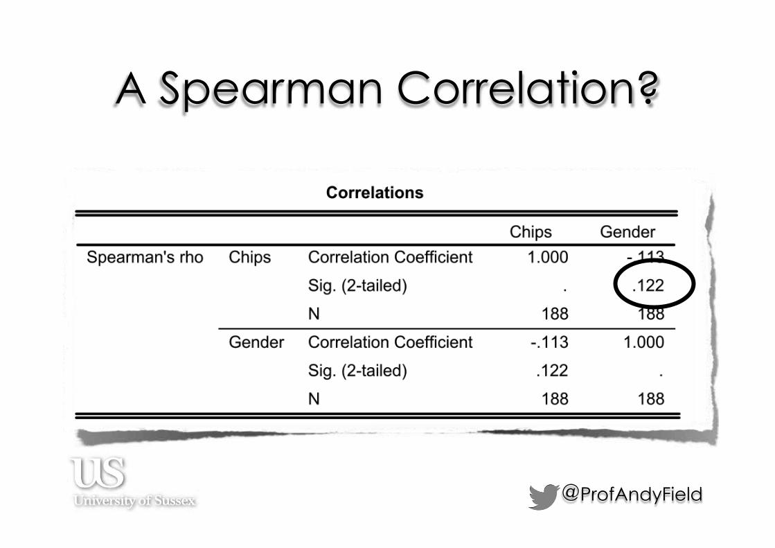
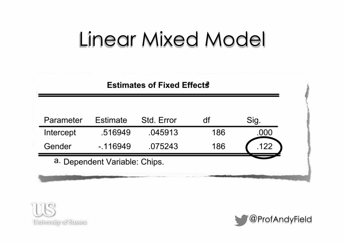
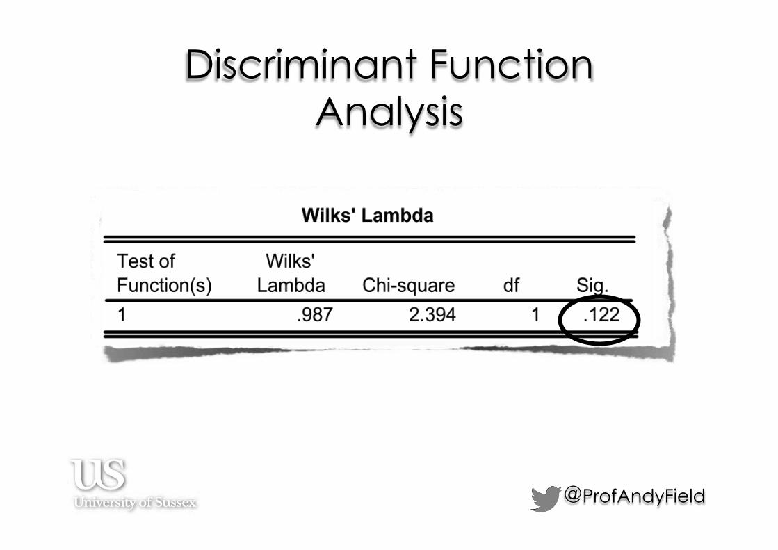
! I collect data about how many humans and zombies choose brain chips or potato chips to accompany their dinner.
! How do I analyze these data?

@ProfAndyField
A Chi-square Test?
@ProfAndyField
A Spearman Correlation?

@ProfAndyField
A Kendall’s Tau-b Correlation?

@ProfAndyField
A (Pearson) Correlation

@ProfAndyField
A t-Test?

@ProfAndyField
Linear Regression?

@ProfAndyField
Wilcoxon-Mann-Whitney Test?

@ProfAndyField
Kruskal-Wallis Test

@ProfAndyField
Logistic Regression

@ProfAndyField
Ordinal Logistic Regression (PLUM)

@ProfAndyField
One-Way ANOVA
@ProfAndyField
Linear Mixed Model
@ProfAndyField
Discriminant Function Analysis


GLM
One
Two or more
Continuous
Categorical
How many outcome variables?
What type of outcome?
How many predictor variables?
What type of predictor?
If a categorical predictor, how
many categories?
If a categorical predictor, are the same or different
entities in each category?
Assumptions of linear model met
Continuous
One
Two or more
One
Two or more
One
Two or more
Continuous
Categorical
Continuous
Categorical
Continuous
Categorical
Both
Continuous
Categorical
Both
Categorical
Categorical
Both
Two
More than two
Different
Same
Different
Same
Different
Same
both
Different
Different
Different
Independent t-test or Point-biserial correlation
Bootstrapped t-test or Mann-Whitney Test
Paired-samples t-test (Dependent t-test)
Bootstrapped t-test or Wilcoxon signed-rank test
One-way independent ANOVA
Robust ANOVA or Kruskal-Wallis test
One-way repeated measures ANOVA
Bootstrapped ANOVA or Friedman's ANOVA
Pearson correlation or regression
Bootstrap correlation/regression, Spearman
correlation, Kendall's tau
Factorial repeated measures ANOVA
Robust factorial repeated measures ANOVA
Multiple regression Bootstrapped multiple regression
Factorial mixed ANOVA Robust factorial mixed ANOVA
Independent factorial ANOVA/multiple regression
Robust independent factorial ANOVA/multiple regression
Multiple regression/ANCOVA Robust ANCOVA/bootstrapped regression
Logistic regression or biserial/point biserial
correlation
Pearson chi-square or likelihood ratio
Logistic regression
Loglinear analysis
MANOVA
Factorial MANOVA
MANCOVA
Assumptions of linear model not met
Logistic regression

@ProfAndyField
The GLM
! The Viagra example from DSUS.
! We can conduct a study measure a person’s libido and partner’s libido over a period following a dose of Viagra. ! Outcome (or DV) = Participant’s libido ! Predictor (or IV) = Dose of Viagra (continuous
or categorical) ! Covariate = Partner’s libido (continuous)
@ProfAndyField
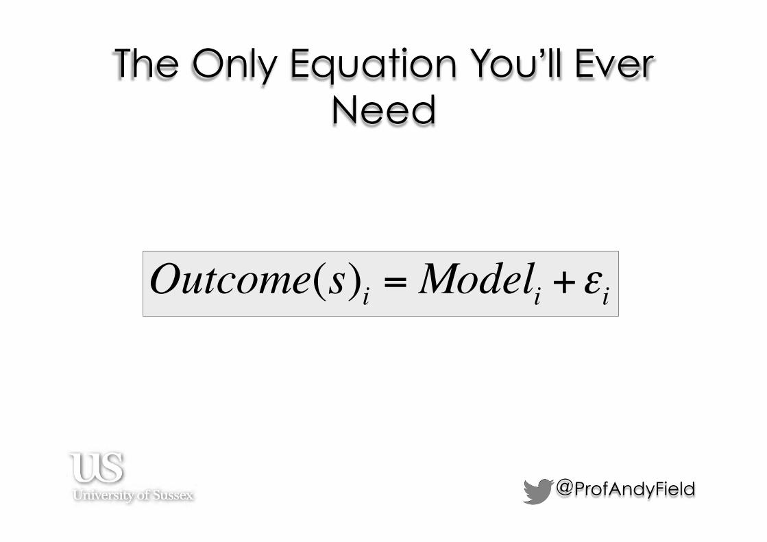
The Only Equation You’ll Ever Need
Outcome(s)i =Modeli +εi

Models Outcomei = b+εiMean
Outcomei = bPredictori +εiCorrelation
Outcomei = b0 + b1Predictori +εiRegression
Outcomei = b0 + b1Predictori +εit-test
Outcomei = b0 + b1Predictor1i + b2Predictor2i +εiRegression
Outcomei = b0 + b1Predictor1i + b2Predictor2i +εiANOVA
Outcomei = b0 + b1Predictori + b2Predictori +εiANCOVA

Models Libidoi = b+εiMean
Libidoi = bDosei +εiCorrelation
Libidoi = b0 + b1Dosei +εiRegression
Libidoi = b0 + b1Dosei +εit-test
Libidoi = b0 + b1Dosei + b2Partneri +εiRegression
Libidoi = b0 + b1Dose1i + b2Dose2i +εiANOVA
Libidoi = b0 + b1Dosei + b2Partneri +εiANCOVA

Complex Models
Outcomei = b0 + b1Ai + b2Bi + b3ABi +εiModeration
Outcomeij = b0 + b1Predictorij +εij + (u0 j )+ (u1 j )Repeated Measures
Outcomei = b0 + b1Ai + b2Bi + b3ABi +εiFactorial ANOVA
Outcomeij = b0 + b1Predictorij +εij + (u0 j )+ (u1 j )Multilevel

@ProfAndyField
F = t2
@ProfAndyField
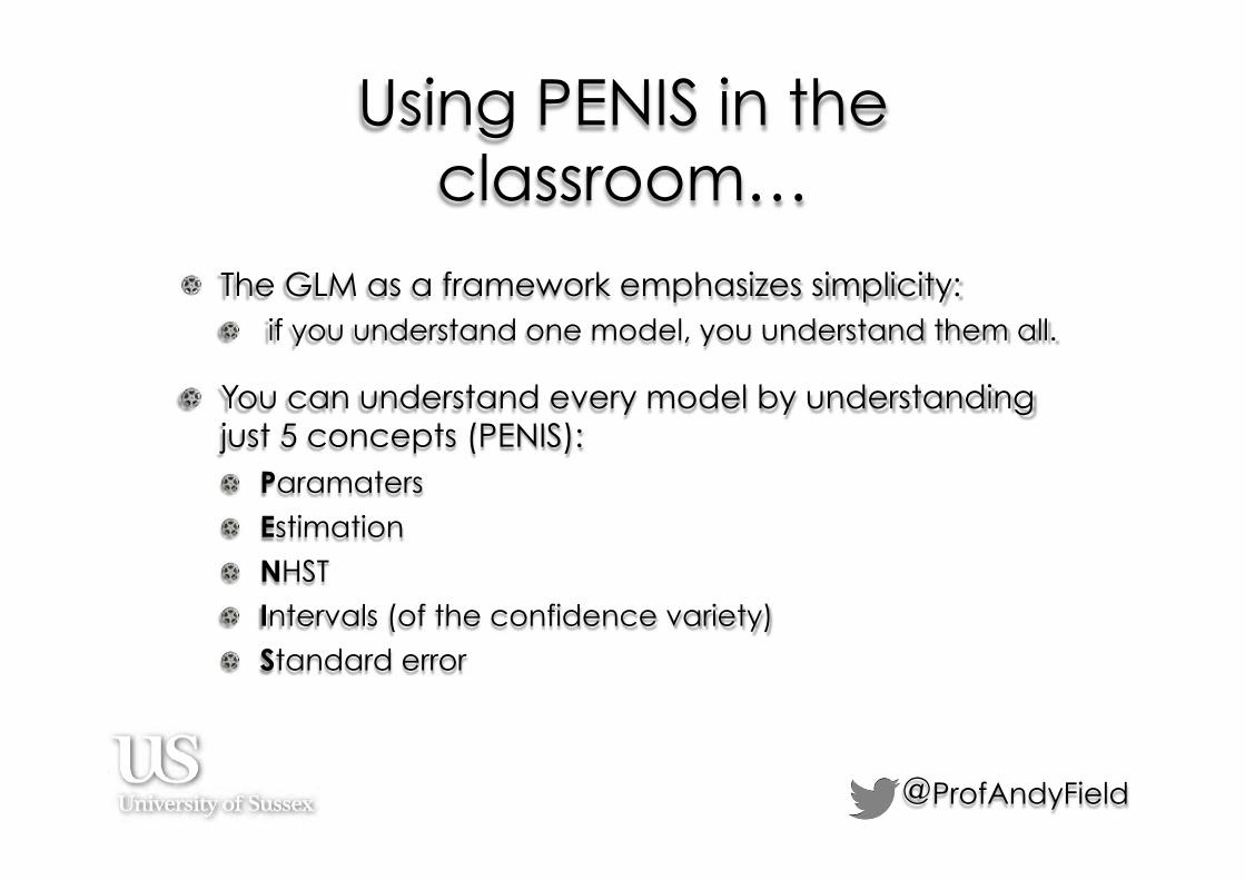
Using PENIS in the classroom…
! The GLM as a framework emphasizes simplicity: ! if you understand one model, you understand them all.
! You can understand every model by understanding just 5 concepts (PENIS): ! Paramaters
! Estimation
! NHST
! Intervals (of the confidence variety)
! Standard error

• Collect some data: • 1, 3, 4, 3, 2 • Add them up:
P: Parameters
• Divide by the number of scores, n:
!! = 1+ 3+ 4+ 3+ 2 = 13!
!!!!
!
! = !!!!!!! = 13
5 = 2.6!

@ProfAndyField
The mean as a model
( ) iii errorModelOutcome +=
( )Bellend Dr.
Bellend Dr.Bellend Dr.
error6.21errorFriends
+=
+= X

@ProfAndyField
A Perfect Fit
1
2
3
4
5 ● ● ● ● ● ● ●
1 2 3 4 5 6 7Rater
Rat
ing
(out
of 5
)

@ProfAndyField
1
2
3
4
5 ●● ● ●●●● ●● ● ● ●● ●● ●● ●●● ●● ●●● ●● ●● ●● ●●●● ●●
● ●●● ●● ●●● ● ●●
● ●
●
● ● ●● ● ●● ●●● ●●● ● ●● ● ●● ●
0 20 40 60Customer
Rat
ing
on a
maz
on.c
o.uk
(out
of 5
)

@ProfAndyField
Calculating ‘Error’ ! A deviation is the difference between the
mean and an actual data point.
! Deviations can be calculated by taking each score and subtracting the mean from it:
xxi −= Deviation

@ProfAndyField
-1.6
-0.6
+0.4 +0.4
+1.4
@ProfAndyField
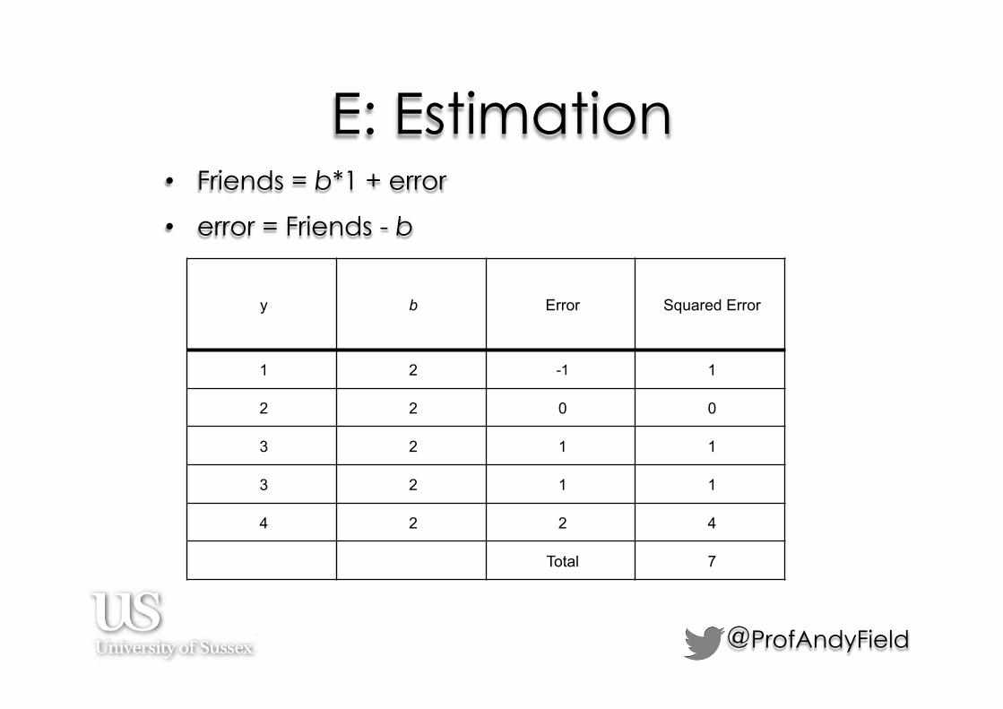
E: Estimation • Friends = b*1 + error
• error = Friends - b
y b Error Squared Error
1 2 -1 1
2 2 0 0
3 2 1 1
3 2 1 1
4 2 2 4
Total 7

Value of b
Sum
of S
quar
ed E
rror
0
5
10
15
20
25
30
35
●
●
●
●
●
●
●
●
●
●
●
●
●
●
●
●
●
●
●
●●
●●
● ● ● ● ● ● ●●
●●
●
●
●
●
●
●
●
●
●
●
●
●
●
●
●
●
●
●
●
●
2.6
0 1 2 3 4 5

Population µ = 3
!!= 3
!!= 3
!!= 3
!!= 4
!!= 4
!!= 2
!!= 2
!!= 5
Mean = 3 SD = 1.22
S: Standard Error

6 7 8 9 10 11 12 13 14 15 16 17 18 19 20 21 22 23
Sperm Count (Millions)
Sample 50Sample 49Sample 48Sample 47Sample 46Sample 45Sample 44Sample 43Sample 42Sample 41Sample 40Sample 39Sample 38Sample 37Sample 36Sample 35Sample 34Sample 33Sample 32Sample 31Sample 30Sample 29Sample 28Sample 27Sample 26Sample 25Sample 24Sample 23Sample 22Sample 21Sample 20Sample 19Sample 18Sample 17Sample 16Sample 15Sample 14Sample 13Sample 12Sample 11Sample 10Sample 9Sample 8Sample 7Sample 6Sample 5Sample 4Sample 3Sample 2Sample 1
These intervals don't contain
the 'true' value
I: Intervals

Sample Number
Sper
m C
ount
(Milli
ons)
0123456789
101112131415161718192021222324252627282930
0123456789
101112131415161718192021222324252627282930
Probability ... .01
●
●
Probability ... .05 (Equal)
●
●
Sample 1 Sample 2
Probability < .01
●
●
Probability ... .05 (Unequal)
●
●
Sample 1 Sample 2
Probability ≈ .01 Probability < .01
Probability ≈ .05Probability ≈ .05
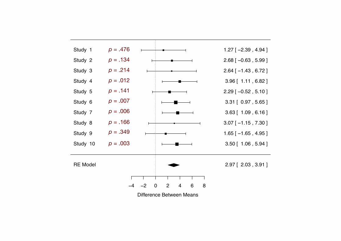
RE Model
−4 −2 0 2 4 6 8
Difference Between Means
Study 10
Study 9
Study 8
Study 7
Study 6
Study 5
Study 4
Study 3
Study 2
Study 1
3.50 [ 1.06 , 5.94 ]
1.65 [ −1.65 , 4.95 ]
3.07 [ −1.15 , 7.30 ]
3.63 [ 1.09 , 6.16 ]
3.31 [ 0.97 , 5.65 ]
2.29 [ −0.52 , 5.10 ]
3.96 [ 1.11 , 6.82 ]
2.64 [ −1.43 , 6.72 ]
2.68 [ −0.63 , 5.99 ]
1.27 [ −2.39 , 4.94 ]
2.97 [ 2.03 , 3.91 ]
p = .476p = .134p = .214p = .012p = .141p = .007p = .006p = .166p = .349
p = .003

@ProfAndyField
N: NHST ! All parameters have an associated distribution.
! Therefore, for any parameter, we can work out the probability of getting at least the value we have if a null hypothesis of interest is true (e.g., if b = 0, or b1 = b2).
! Distributions might have different symbols to represent them, but they mean the same thing.
z
Density
0.00
0.05
0.10
0.15
0.20
0.25
0.30
0.35
0.40
●●●●●●●●●●●●●●●●●●●●●●●●●●●●●●●●●●●●●●●●●●●●●●●●●●●●●●●●●●●●●●●●●●●●●●●●●●●●●●●●●●●●●●●●●●●●●●●●●●●●●●●●●●●●●●●●
●●●●●●●●●●●●●●●●●●●●●●●●●
●●●●●●●●●●●●●●●●●●●●●●●●●●●●●●●●●●●●●●●●●●●●●●●●●●●●●●●●●●●●●●●●●●●●●●●●●●●●●●●●●●●●●●●●●●●●●●●●●●●●●●●●●●●●●●●●●●●●●●●●●●●●●●●●●●●●●●●●●●●●●●●●●●●●●●●●●●●●●●●●●●●●●●●●●●●●●●●●●●●●●●●●●●●●●●●●●●●●●●●●●●●●●●●●●●●●●●●●●●●●●●●●●●●●●●●●●●●●●●●●●●●●●●●●●●●●●●●●●●●●●●●●●●●●●●●●●●●●●●●●●●●●●●●●●●●●●●●●●●●●●●●●●●●●●●●●●●●●●●●●●●●●●●●●●●●●●●●●●●●●●●●●●●●●●●●●●●●●●●●●●●●●●●●●●●●●●●●●●●●●●●●●●●●●●●●●●●●●●●●●●●●●●●●●●●●●●●●●●●●●●●●●●●●●●●●●●●●●●●●●●●●●●●●●●●●●●●●●●●●●●●●●●●●●●●●●●●●●●●●●●●●●●●●●●●●●●●●●●●●●●●●●●●●●●●●●●●●●●●●●●●●●●●●●●●●●●●●●●●●●●●●●●●●●●●●●●●●●●●●●●●●●●●●●●●●●●●●●●●●●●●●●●●●●●●●●●●●●●●●●●●●●●●●●●●●●●●●●●●●●●●●●●●●●●●●●●●●●●●●●●●●●●●●●●●●●●●●●●●●●●●●●
−4.00 −3.00 −1.96 −1.00 0.00 1.00 1.65 1.96 3.00 4.00
Probability = .025 Probability = .025
Probability = .95

@ProfAndyField
Snowballing Simplicity ! Homoscedasticity/Homogeneity of variance
! In large samples do not bias bs (CLT applies), but are important for OLS estimation to be optimal.
! Bias Standard Errors (hence CIs and ps)
! Normality (of sampling distribution/residuals) ! b are optimal in OLS estimation when residuals normal. ! CIs and ps of bs not biased if the sample is big enough (CLT)
! Outliers ! Bias Means and Variance/SS
! Bias tests of parameters (low power) ! Bias parameter/Effect size estimates
! Remedies ! Any parameter/CI can be bootstrapped (no need for nonparametric
stats) ! Adjust the data (transform, windzorize, trim)

@ProfAndyField
Summary ! The GLM is a useful framework for teaching statistics
! It enables you to get your PENIS out in lectures without getting arrested.
! If you understand the PENIS, you understand any statistical model: ! All models have parameters that define the model and tell
you about your hypothesis ! These parameters are estimated ! They vary in samples ! They tell us about the ‘true’ size of the effect (Cis) ! They can be significance tested ! They (and their CIs and p-values) can be biased ! They (and their CIs) can be bootstrapped

@ProfAndyField
My statistics cult:
@ProfAndyField
www.facebook.com/ProfAndyField
discoveringstatistics.blogspot.co.uk
www.youtube.com/user/profandyfield


