Policy Research Working Paper 9278 Malaysia’s Economic Growth and Transition to High Income An Application of the World Bank Long Term Growth Model (LTGM) Sharmila Devadas Jorge Guzman Young Eun Kim Norman Loayza Steven Pennings Development Economics Development Research Group June 2020 Public Disclosure Authorized Public Disclosure Authorized Public Disclosure Authorized Public Disclosure Authorized
Transcript
Policy Research Working Paper 9278
Malaysia’s Economic Growth and Transition to High Income
An Application of the World Bank Long Term Growth Model (LTGM)
Sharmila DevadasJorge Guzman
Young Eun KimNorman Loayza Steven Pennings
Development Economics Development Research GroupJune 2020
Pub
lic D
iscl
osur
e A
utho
rized
Pub
lic D
iscl
osur
e A
utho
rized
Pub
lic D
iscl
osur
e A
utho
rized
Pub
lic D
iscl
osur
e A
utho
rized
Produced by the Research Support Team
Abstract
The Policy Research Working Paper Series disseminates the findings of work in progress to encourage the exchange of ideas about development issues. An objective of the series is to get the findings out quickly, even if the presentations are less than fully polished. The papers carry the names of the authors and should be cited accordingly. The findings, interpretations, and conclusions expressed in this paper are entirely those of the authors. They do not necessarily represent the views of the International Bank for Reconstruction and Development/World Bank and its affiliated organizations, or those of the Executive Directors of the World Bank or the governments they represent.
Policy Research Working Paper 9278
This paper studies economic growth in Malaysia, with the purpose of assessing the potential to attain the status and characteristics of a high-income country. Future economic growth is simulated under a business-as-usual baseline, where the growth drivers follow their historical or recent trends, and under different scenarios of reform, using the World Bank Long-Term Growth Model (LTGM). Under the business-as-usual baseline, Malaysia’s GDP growth is expected to decline from 4.5 to 2.0 percent over the next three decades, following the country’s transition to high income in 2024 (which might be delayed due to the effects
of COVID-19). This decline is partly due to demographics, but also a declining marginal product of private capital and slowing growth rates of total factor productivity and human capital. Strong reforms are required for Malaysia to grow beyond what is expected based on historical trends, espe-cially for human capital, female labor force participation, and total factor productivity. In the strong reform scenario, based on growth drivers achieving a target corresponding to the 75th percentile of high-income countries, GDP growth is expected to have a substantially higher trajectory, reaching 3.6 percent by 2050.
This paper is a product of the Development Research Group, Development Economics. It is part of a larger effort by the World Bank to provide open access to its research and make a contribution to development policy discussions around the world. Policy Research Working Papers are also posted on the Web at http://www.worldbank.org/prwp. The authors may be contacted at [email protected], [email protected], [email protected], [email protected], and [email protected].
Malaysia’s Economic Growth and Transition to High Income:
An Application of the World Bank Long Term Growth Model (LTGM)
Sharmila Devadas Jorge Guzman Young Eun Kim Norman Loayza Steven Pennings
Development Research Group
The World Bank
.
Keywords: Economic growth, human capital, investment, labor force participation, total factor productivity, innovation, education, market efficiency, infrastructure, institutions, Malaysia
Note: The views expressed herein are those of the authors and do not necessarily reflect the views of the World Bank, its Executive Directors, or the countries they represent. We appreciate comments from Yew Keat Chong, Firas Raad, Richard Record, Shakira Binti Teh Sharifuddin, and seminar participants at the World Bank. To download the Long Term Growth Models, visit www.worldbank.org/LTGM
2
Introduction
Over the past few decades, Malaysia has recorded strong and sustained growth, apart from during periods
such as the Asian financial crisis in 1997, the global financial crisis in 2009 and – more recently – the
COVID-19 pandemic in 2020 (Figure 1.1). As the economic effects of the COVID-19 pandemic will
hopefully be short-lived, this paper looks through the current growth volatility to focus on long-run trends.
Malaysia’s long-run growth performance has supported remarkable gains in social and economic
development, with a nine-fold increase in per capita income over the last seven decades. The country is
expecting to transition to high-income status in the near future (Figure 1.2), where high income is based
on the World Bank’s cross-country classification. This paper studies Malaysia’s long-run economic
growth prospects as it attains the status and characteristics of a high-income economy.
Figure 1.1. Historical GDP Growth Figure 1.2. Historical Real GNI Per Capita Level1
The Government of Malaysia’s long-run and medium-run growth strategies are outlined in its Shared
Prosperity Vision (SPV) 2030 and 12th Malaysia Plan (respectively). The SPV and Malaysia plan go
beyond high-income status, also ensuring growth is both sustainable and equitable. The October 2019
SPV sets out “a commitment to make Malaysia a nation that achieves sustainable growth along with fair
and equitable distribution.” 2 The SPV blueprint proposes targets across key growth areas: regional
inclusion, the role of SMEs, human capital, labor market and workers’ compensation, and social capital
and well-being. The 12th Malaysia Plan, the next five-year national development plan, is slated for 2021-
2025, and will be released in 2020. It aims to be aligned to SPV 2030, covering the areas of economic
1 Methodology for Figure 1.2: Calibrate the levels to GNI per capita Atlas method (NY.GNP.PCAP.CD) for 2018, and then cast backwards using real GNI growth (NY.GNP.PCAP.KD.ZG). Dotted line shown is the 2019-20 high income threshold. 2 The new government that assumed administration at the end of February 2020 has pledged to ensure the continuity of SPV 2030.
3
empowerment (growth drivers and enablers), environmental sustainability, and social re-engineering
(essentially improving the well-being of the people and social cohesion).
This paper simulates Malaysia’s long-run growth prospects using the World Bank Long-Term Growth
Model (LTGM), a suite of spreadsheet-based tools building on the celebrated Solow-Swan growth model
(Loayza and Pennings 2018, and Hevia and Loayza 2012). The Long-Term Growth Model – Public
Capital Extension (LTGM-PC) is used as the base model (Devadas and Pennings 2018), which allows for
private and public investment to have different effects on growth. Human capital and TFP growth are
endogenized using LTGM’s Human Capital extension (LTGM-HC) and TFP extension (LTGM-TFP),
respectively. The LTGM-HC combines average years of schooling by age cohort with the quality of
education and health components to determine human capital. In the LTGM-TFP (Kim and Loayza 2018),
the TFP growth rate is calculated as the composite effect of TFP determinants: innovation, education,
market efficiency, infrastructure, and institutions. The models are described in more detail in Appendix 1
and most are available for download at www.worldbank.org/LTGM.
Our first result concerns a Malaysia’s business-as-usual baseline growth path, where the growth drivers
─public and private investment-to-GDP ratios, total factor productivity (TFP), human capital, and labor
force participation rates ─ follow their historical or recent trends (future demographic projections taken
from the United Nations (UN). We find trend GDP growth in Malaysia is likely to fall from around 4.5
percent in 2020 to 2.0 percent in 2050, driven mostly by demographics, falling private investment
effectiveness and declining TFP growth. Declining growth is common among peer countries as they
transition to high-income status.
However, this decline is growth is not destiny, and our second finding is that it can be partially offset by
economic reforms. Specifically, we simulate weak, moderate, and strong reforms for each growth driver,
with targets set with reference to the distribution of those values among high-income (HI) countries. While
weak reforms have little effect (relative to the baseline), moderate and strong reforms generate growth in
2050 that is 1.5 to 1.8 times that in the business-as-usual baseline (respectively).
The rest of the paper is organized as follows. Section 1 presents the historical developments for each
growth driver. Section 2 discusses the assumptions regarding growth drivers and parameters used in the
baseline simulation. Section 3 shows the baseline GDP growth trajectory over the next three decades and
analyzes the contribution of each growth driver to both current growth rates and changes in the growth
rate over 2020-50. Section 4 presents the impact on GDP growth of the different levels of reforms for each
determinant of growth: “weak” reform benchmarking at the 25th percentile among high-income countries;
“moderate” reform, at the 50th percentile; and “strong” reform, at the 75th percentile. Section 5 discusses
the implications for GDP growth when the effects of all growth drivers are combined for each scenario of
weak, moderate, and strong reform. The conclusion provides a summary of main findings and policy
implications.
1. Historical developments in growth drivers
In this section we review the historical drivers of growth in Malaysia through the lens of LTGM. First, we
describe historical trends in GDP growth and GDP per capita growth, which provide context for future
growth performance. Then we discuss the historical path of the investment-to-GDP ratios (both public and
private), TFP growth, human capital growth, demographics, and the labor force participation rate, which
help us calibrate the future paths of these growth drivers.
Post-2000, GDP growth in Malaysia has averaged 5% (Figure 1.1), but growth has slowed relative to the
faster rate in the 1990s. Slower growth rates as countries develop are however common, as we discuss in
more detail in Section 3. Malaysia has also experienced a relatively steady rate of per capita GDP growth
of 3.3% over the past 20 years. These growth rates have allowed the real GNP per capita level to double
since the mid-1990s. However, otherwise steady growth has been marked by slowdowns resulting from
the Asian Financial Crisis in 1997, the 2009 Global Financial Crisis, earlier recessions around 1985 and
1975, and the recent 2020 COVID-19 pandemic (based on forecasts).
Figure 1.3. Historical Investment-to-GDP (%) Figure 1.4. Historical Public and Private Investment-to-GDP (%)
High income status is defined by the World Bank as countries with GNI per capita above $12,376 in 2019-
20 (measured at Atlas exchange rates). In 2018, Malaysia’s GNI per capita was at $10,460 (Figure 1.2)
5
and historical trends suggest that Malaysia is expected to pass the threshold in the mid-2020s. However,
this projection might be delayed due to the effect of COVID-19, causing a reduction in the forecasted
growth in 2020 and possibly in the early 2020s (Figure 1.1).3
Aggregate investment-to-GDP has averaged 24% over the last two decades (Figure 1.3), with public
investment trending down and private investment trending up (Figure 1.4). During the late 1980s and
1990s, investment rates in Malaysia increased rapidly, reaching over 40% of GDP just before the 1997
Asian financial crisis. High private investment-to-GDP rates were buoyed by the First Industrial Master
Plan (1986-1995), and liberalization and deregulation in the economy. In the 1990s, excessive investments
also occurred in certain sectors, especially the property sector. After the Asian financial crisis, the
investment-to-GDP ratio declined, with the fall mostly due to lower levels of private investment (not
shown). In the last 10 years, investment-to-GDP has averaged 24.6%. A closer look at the split between
public and private investment shows that public investment has been declining since 2012, falling from
around 11% to 7% of GDP in 2018. This is reflective of the government’s fiscal consolidation plan. At
the same time, some rebalancing has been observed with private investment rising from 15% to 17% of
GDP.
The median TFP growth over the past 30 years (1985-2014) is 0.9% (Figure 1.5). Since TFP is calculated
as a residual – growth less factor accumulation – it is volatile and oscillates with the economic cycle.
The human capital growth rate has experienced a downward trend since the early 1990s and it has averaged
roughly 0.6-0.7% in the 2010-2014 period (Figure 1.6). Human capital is a commonly measured using the
average years of schooling, though in our forward-looking simulations we use a broader measure based
on the World Bank Human Capital Index that includes schooling quality and population health. In the
1980s and early 1990s, human capital grew at around 2% but now has slowed to 0.6%. As it is harder to
increase the average years of education when people are already well educated, countries often experience
a slowing growth rate of human capital over time. We expect this trend will continue for Malaysia as it
moves to high income status.
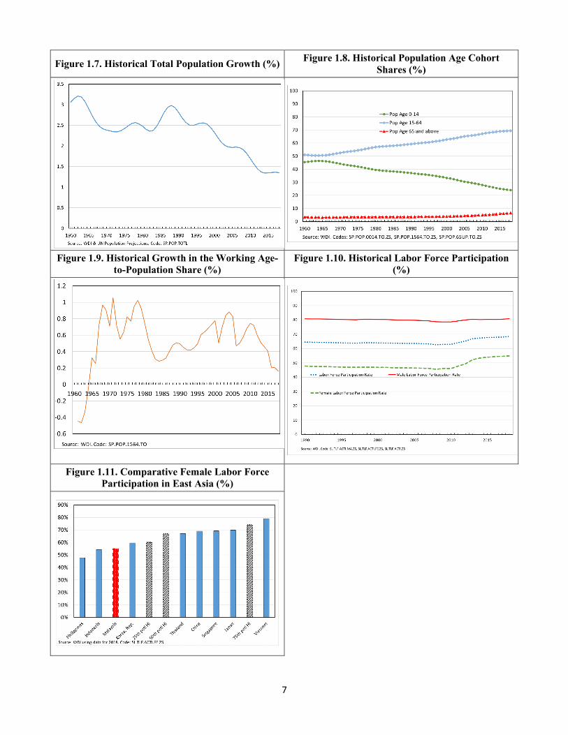
Total population growth was close to 1.3% over the past 5 years, after experiencing a downward trend
since 1990 (Figure 1.7). Before 1990, population growth averaged 2.5-3%. Slower population growth is
typical of developing economies that transition into high-income economies and is expected to continue.
Slowing population growth also affects the share of population of working age (15-64), which in turn
affects the size of the labor force (Figure 1.8). The share of the population between the ages 0 to 14 has
3 World Bank (2020) projects a growth rate of -0.1% under the baseline and -4.6% under a low-case scenario for 2020.
6
been declining, due to falling fertility, which has led to a “demographic dividend”: the share of the
population of working age grew by around 0.6% over 1965-2010, and then accelerated to 1% in the 2000s
(Figure 1.9). Analytically, the LTGM suggests this demographic dividend contributed at least 0.3ppts to
GDP growth throughout this period.4 Since 2010, we can observe a declining growth rate of the share of
the population of working age (Figure 1.9), which has recently approached zero. This is the result of an
aging population --- fewer children and longer life expectancy ---and is a characteristic of an economy
transitioning to high income status. Examples of population aging can be found in developed economies
like Japan, the Republic of Korea and Western Europe, and is expected to continue.
Figure 1.5. Historical TFP Growth Figure 1.6. Historical Human Capital Growth
Historically, the labor force participation rate has been stable at around 64%, until 2010 when it increased
to 68% by 2018 (Figure 1.10). This is mostly due to higher female labor force participation (FLFP), which
increased from about 46% in the 1990-2010 period to 55% by 2018. In contrast, male labor force
participation has remained relatively constant at around 80% since 1990. Despite the increase in recent
years, Malaysia’s FLFP is still lagging its regional peers like Thailand, China, and Singapore and as well
as high-income peers (Figure 1.11). Higher rates of FLFP increase the labor supply in the economy, and
hence the level of GDP per capita.
4 Analytically, the 0.6ppts of growth in the working age to total population ratio will be multiplied by the labor share of income, which is 50%, resulting in about 0.3ppts to GDP growth each year.
7
Figure 1.7. Historical Total Population Growth (%) Figure 1.8. Historical Population Age Cohort Shares (%)
Figure 1.9. Historical Growth in the Working Age-to-Population Share (%)
Figure 1.10. Historical Labor Force Participation (%)
Figure 1.11. Comparative Female Labor Force Participation in East Asia (%)
8
2. Growth drivers in the business-as-usual baseline
In this section we explore the assumptions that are required to calibrate the LTGM-PC to simulate
Malaysia’s business-as-usual baseline over 2020-50. To create a business-as-usual baseline for the
Malaysian economy in the long run, we need to calibrate the future paths of the growth drivers like
investment, the growth of both TFP and human capital, as well as other key parameters. These assumptions
are summarized in Table 2.1. We calibrate the LTGM-PC as the foundation of the analysis and add the
LTGM-TFP extension and the LTGM-HC extension to simulate TFP growth and human capital growth,
respectively. Additionally, short-to-medium term forecasts produced by the IMF in its Article IV report
help us calibrate the future paths of public and private investment. We use population growth projections
(by age cohort) from the UN for demographic trends until 2050. The remaining projections are determined
by assuming that long-term trends in Malaysia remain constant and by performing some steady state
calculations. The labor share of income is calibrated to 50%, which is close to its value from Penn World
Tables version 9.0 (PWT 9).
Table 2.1. Summary of Assumptions for the Malaysia Business-as-Usual Baseline
Variable Baseline Source/Comments Labor Share 50.0% Similar to the 2014 PWT 9 figure of 53% Depreciation Rate (aggregate) 5.8% PWT 9 figure for 2014 Capital-to-Output Ratio 2.25 At steady state value Human Capital Growth 0.6% ̶ 0.1% Calculated using the LTGM Human Capital Extension
TFP Growth 0.9% ̶ 0.6% Similar to the last 15-year average and the last 30-year median using PWT 9
Investment-to-GDP Ratio 24% Based on projections of public and private-investment-to-GDP
Public Investment-to-GDP Ratio 6.0% Based on recent trend and IMF projection up to 2023 Private Investment-to-GDP Ratio 18.0% Based on recent trend and IMF projection up to 2023 Population Growth 1.3% ̶ 0.4% UN Population projections (via WB HDN)
GDP Growth 2020-50 4.5% ̶ 2.0% 4.6% is MTI forecast for 2020 and 4.8% is the IMF Oct. 2019 WEO projections average for 2020-23.
Atlas GNI PC Level US$ 10,460 World Bank WDI for 2018
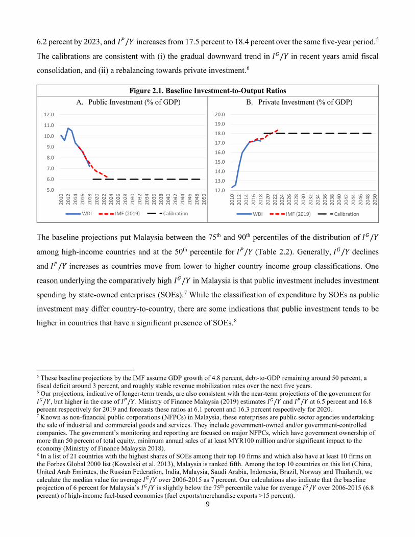
Investment-to-GDP is assumed to remain around 24% given recent trends and the IMF Article IV
projections for the next few years. For the baseline, we calibrate public investment-to-output and private
investment-to-output ratios (𝐼𝐼𝐺𝐺/𝑌𝑌 and 𝐼𝐼𝑃𝑃/𝑌𝑌) of 6 percent and 18 percent respectively (Figure 2.1). This is
based on projections made by IMF (2019), which forecast that 𝐼𝐼𝐺𝐺/𝑌𝑌 declines from 7 percent in 2019 to
9
6.2 percent by 2023, and 𝐼𝐼𝑃𝑃/𝑌𝑌 increases from 17.5 percent to 18.4 percent over the same five-year period.5
The calibrations are consistent with (i) the gradual downward trend in 𝐼𝐼𝐺𝐺/𝑌𝑌 in recent years amid fiscal
consolidation, and (ii) a rebalancing towards private investment.6
Figure 2.1. Baseline Investment-to-Output Ratios A. Public Investment (% of GDP) B. Private Investment (% of GDP)
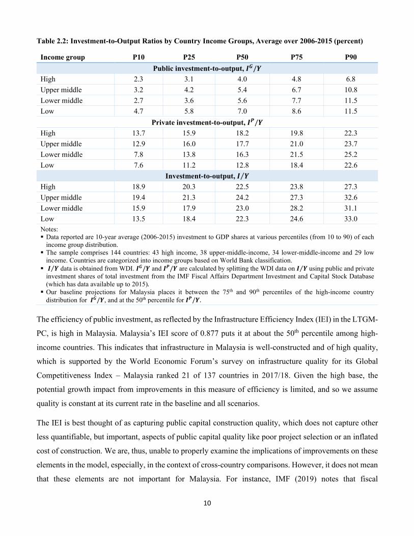
The baseline projections put Malaysia between the 75th and 90th percentiles of the distribution of 𝐼𝐼𝐺𝐺/𝑌𝑌
among high-income countries and at the 50th percentile for 𝐼𝐼𝑃𝑃/𝑌𝑌 (Table 2.2). Generally, 𝐼𝐼𝐺𝐺/𝑌𝑌 declines
and 𝐼𝐼𝑃𝑃/𝑌𝑌 increases as countries move from lower to higher country income group classifications. One
reason underlying the comparatively high 𝐼𝐼𝐺𝐺/𝑌𝑌 in Malaysia is that public investment includes investment
spending by state-owned enterprises (SOEs).7 While the classification of expenditure by SOEs as public
investment may differ country-to-country, there are some indications that public investment tends to be
higher in countries that have a significant presence of SOEs.8
5 These baseline projections by the IMF assume GDP growth of 4.8 percent, debt-to-GDP remaining around 50 percent, a fiscal deficit around 3 percent, and roughly stable revenue mobilization rates over the next five years. 6 Our projections, indicative of longer-term trends, are also consistent with the near-term projections of the government for 𝐼𝐼𝐺𝐺/𝑌𝑌, but higher in the case of 𝐼𝐼𝑃𝑃/𝑌𝑌. Ministry of Finance Malaysia (2019) estimates 𝐼𝐼𝐺𝐺/𝑌𝑌 and 𝐼𝐼𝑃𝑃/𝑌𝑌 at 6.5 percent and 16.8 percent respectively for 2019 and forecasts these ratios at 6.1 percent and 16.3 percent respectively for 2020. 7 Known as non-financial public corporations (NFPCs) in Malaysia, these enterprises are public sector agencies undertaking the sale of industrial and commercial goods and services. They include government-owned and/or government-controlled companies. The government’s monitoring and reporting are focused on major NFPCs, which have government ownership of more than 50 percent of total equity, minimum annual sales of at least MYR100 million and/or significant impact to the economy (Ministry of Finance Malaysia 2018). 8 In a list of 21 countries with the highest shares of SOEs among their top 10 firms and which also have at least 10 firms on the Forbes Global 2000 list (Kowalski et al. 2013), Malaysia is ranked fifth. Among the top 10 countries on this list (China, United Arab Emirates, the Russian Federation, India, Malaysia, Saudi Arabia, Indonesia, Brazil, Norway and Thailand), we calculate the median value for average 𝐼𝐼𝐺𝐺/𝑌𝑌 over 2006-2015 as 7 percent. Our calculations also indicate that the baseline projection of 6 percent for Malaysia’s 𝐼𝐼𝐺𝐺/𝑌𝑌 is slightly below the 75th percentile value for average 𝐼𝐼𝐺𝐺/𝑌𝑌 over 2006-2015 (6.8 percent) of high-income fuel-based economies (fuel exports/merchandise exports >15 percent).
5.0
6.0
7.0
8.0
9.0
10.0
11.0
12.0
2010
2012
2014
2016
2018
2020
2022
2024
2026
2028
2030
2032
2034
2036
2038
2040
2042
2044
2046
2048
2050
WDI IMF (2019) Calibration
12.0
13.0
14.0
15.0
16.0
17.0
18.0
19.0
20.0
2010
2012
2014
2016
2018
2020
2022
2024
2026
2028
2030
2032
2034
2036
2038
2040
2042
2044
2046
2048
2050
WDI IMF (2019) Calibration
10
Table 2.2: Investment-to-Output Ratios by Country Income Groups, Average over 2006-2015 (percent)
Income group P10 P25 P50 P75 P90 Public investment-to-output, 𝑰𝑰𝑮𝑮/𝒀𝒀
Investment-to-output, 𝑰𝑰 𝒀𝒀⁄ High 18.9 20.3 22.5 23.8 27.3 Upper middle 19.4 21.3 24.2 27.3 32.6 Lower middle 15.9 17.9 23.0 28.2 31.1 Low 13.5 18.4 22.3 24.6 33.0 Notes: Data reported are 10-year average (2006-2015) investment to GDP shares at various percentiles (from 10 to 90) of each
income group distribution. The sample comprises 144 countries: 43 high income, 38 upper-middle-income, 34 lower-middle-income and 29 low
income. Countries are categorized into income groups based on World Bank classification. 𝑰𝑰 𝒀𝒀⁄ data is obtained from WDI. 𝑰𝑰𝑮𝑮/𝒀𝒀 and 𝑰𝑰𝑷𝑷/𝒀𝒀 are calculated by splitting the WDI data on 𝑰𝑰 𝒀𝒀⁄ using public and private
investment shares of total investment from the IMF Fiscal Affairs Department Investment and Capital Stock Database (which has data available up to 2015). Our baseline projections for Malaysia places it between the 75th and 90th percentiles of the high-income country
distribution for 𝑰𝑰𝑮𝑮/𝒀𝒀, and at the 50th percentile for 𝑰𝑰𝑷𝑷/𝒀𝒀. The efficiency of public investment, as reflected by the Infrastructure Efficiency Index (IEI) in the LTGM-
PC, is high in Malaysia. Malaysia’s IEI score of 0.877 puts it at about the 50th percentile among high-
income countries. This indicates that infrastructure in Malaysia is well-constructed and of high quality,
which is supported by the World Economic Forum’s survey on infrastructure quality for its Global
Competitiveness Index – Malaysia ranked 21 of 137 countries in 2017/18. Given the high base, the
potential growth impact from improvements in this measure of efficiency is limited, and so we assume
quality is constant at its current rate in the baseline and all scenarios.
The IEI is best thought of as capturing public capital construction quality, which does not capture other
less quantifiable, but important, aspects of public capital quality like poor project selection or an inflated
cost of construction. We are, thus, unable to properly examine the implications of improvements on these
elements in the model, especially, in the context of cross-country comparisons. However, it does not mean
that these elements are not important for Malaysia. For instance, IMF (2019) notes that fiscal
11
vulnerabilities include reliance on off-budget spending, and weaknesses in project appraisal, approval and
costing (Malaysia scores lower than the OECD average in terms of its procurement systems).
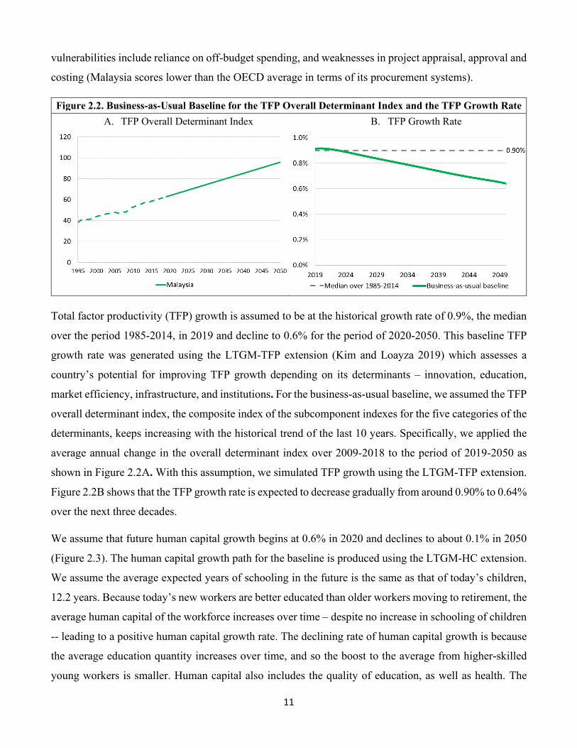
Figure 2.2. Business-as-Usual Baseline for the TFP Overall Determinant Index and the TFP Growth Rate A. TFP Overall Determinant Index B. TFP Growth Rate
Total factor productivity (TFP) growth is assumed to be at the historical growth rate of 0.9%, the median
over the period 1985-2014, in 2019 and decline to 0.6% for the period of 2020-2050. This baseline TFP
growth rate was generated using the LTGM-TFP extension (Kim and Loayza 2019) which assesses a
country’s potential for improving TFP growth depending on its determinants – innovation, education,
market efficiency, infrastructure, and institutions. For the business-as-usual baseline, we assumed the TFP
overall determinant index, the composite index of the subcomponent indexes for the five categories of the
determinants, keeps increasing with the historical trend of the last 10 years. Specifically, we applied the
average annual change in the overall determinant index over 2009-2018 to the period of 2019-2050 as
shown in Figure 2.2A. With this assumption, we simulated TFP growth using the LTGM-TFP extension.
Figure 2.2B shows that the TFP growth rate is expected to decrease gradually from around 0.90% to 0.64%
over the next three decades.
We assume that future human capital growth begins at 0.6% in 2020 and declines to about 0.1% in 2050
(Figure 2.3). The human capital growth path for the baseline is produced using the LTGM-HC extension.
We assume the average expected years of schooling in the future is the same as that of today’s children,
12.2 years. Because today’s new workers are better educated than older workers moving to retirement, the
average human capital of the workforce increases over time – despite no increase in schooling of children
-- leading to a positive human capital growth rate. The declining rate of human capital growth is because
the average education quantity increases over time, and so the boost to the average from higher-skilled
young workers is smaller. Human capital also includes the quality of education, as well as health. The
12
health of the population is measured by adult survival rates (ASRs), which is the probability that a 15-
year-old will reach their 60th birthday, and stunting rates, defined as the fraction of 5 years old that are not
In the baseline, we assume that schooling quality remains at its original level of 0.75, ASRs stay at 0.88
and the not stunted rate stays at 0.79. Data on the health and education variables are taken from the World
Bank’s Human Capital Project.9 Due to a lack of historical data, we also assume that those rates apply to
the whole working-age population, and so schooling quality and health make no contribution to human
capital growth in the baseline. In terms of growth rates, human capital grows at about 0.6% in 2019-2020
and it slowly declines to under 0.1% by 2050. The return to education is assumed to be 12%.
Figure 2.3. Baseline Simulation of Human Capital Growth
The capital-to-output ratio is assumed to be at its steady state value of around 2.3. The steady state capital-
to-output ratio is calculated as the ratio of the investment share of GDP to the sum of trend GDP growth
and depreciation rate (see equation below).10 We divide total capital into public and private shares from
the IMF Fiscal Affairs Department Investment and Capital Stock Database 2017, resulting in 1.14 for the
public capital-to-output ratio (Kg/Y) and 1.11 for the private capital-to-output ratio (Kp/Y), respectively.
9 See https://www.worldbank.org/humancapital. 10 The GDP growth rate used is the average of 4.6% in the past 10 years, and the depreciation rate 5.8% from PWT 9. An alternative approach is to calibrate the capital-to-output ratio using Penn World Tables data, which would have generated a total capital-to-output ratio of around 3, and a lower growth rate over the next few years. But that growth rate was inconsistent with other information, such as recent growth history and forecasts by policy institutions, so we chose the steady-state approach instead.
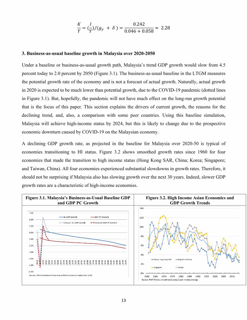
3. Business-as-usual baseline growth in Malaysia over 2020-2050
Under a baseline or business-as-usual growth path, Malaysia’s trend GDP growth would slow from 4.5
percent today to 2.0 percent by 2050 (Figure 3.1). The business-as-usual baseline in the LTGM measures
the potential growth rate of the economy and is not a forecast of actual growth. Naturally, actual growth
in 2020 is expected to be much lower than potential growth, due to the COVID-19 pandemic (dotted lines
in Figure 3.1). But, hopefully, the pandemic will not have much effect on the long-run growth potential
that is the focus of this paper. This section explains the drivers of current growth, the reasons for the
declining trend, and, also, a comparison with some peer countries. Using this baseline simulation,
Malaysia will achieve high-income status by 2024, but this is likely to change due to the prospective
economic downturn caused by COVID-19 on the Malaysian economy.
A declining GDP growth rate, as projected in the baseline for Malaysia over 2020-50 is typical of
economies transitioning to HI status. Figure 3.2 shows smoothed growth rates since 1960 for four
economies that made the transition to high income status (Hong Kong SAR, China; Korea; Singapore;
and Taiwan, China). All four economies experienced substantial slowdowns in growth rates. Therefore, it
should not be surprising if Malaysia also has slowing growth over the next 30 years. Indeed, slower GDP
growth rates are a characteristic of high-income economies.
Figure 3.1. Malaysia’s Business-as-Usual Baseline GDP and GDP PC Growth
Figure 3.2. High Income Asian Economics and GDP Growth Trends
14
What explains current trend growth rates?
Private investment, followed by productivity growth, are the largest drivers of current economic growth.
Current growth rates can be decomposed using a log-linear approximation of the production function as
in Devadas and Pennings (2019) (Equation 16). Private investment is the most important growth driver,
with a net contribution of about 2ppts of the current 4.5 percent GDP growth (Figure 3.3, graph A). Private
investment makes such a large contribution because of the current low private capital-to-output ratio –
driven by many years of low private investment following the Asian Financial Crisis – which increases
the current marginal product of private capital (Figure 3.3, graph B). Note, however, that both the marginal
product and growth contributions change over time, which we discuss in detail below. After private
investment, the next largest contribution is from TFP growth, with a contribution of 0.9ppts. Next,
population growth and public investment each contribute around 0.65ppts, with human capital growth
contributing 0.3ppts.11
Figure 3.3. Net Investment Contribution to GDP Growth and Marginal Product of Capital A. Net Investment Contribution to GDP Growth 1/ B. Marginal Product of Capital
1/ Net public investment contribution to GDP growth ≈ 𝜙𝜙 � 𝐻𝐻𝑡𝑡
𝐺𝐺 𝑌𝑌𝑡𝑡�𝐾𝐾𝑡𝑡𝐺𝐺𝐺𝐺 𝑌𝑌𝑡𝑡�
− 𝛿𝛿𝐺𝐺�.
Net private investment contribution to GDP growth ≈(1 − 𝛽𝛽 − 𝜙𝜙) � 𝐻𝐻𝑡𝑡𝑃𝑃 𝑌𝑌𝑡𝑡�𝐾𝐾𝑡𝑡𝑃𝑃 𝑌𝑌𝑡𝑡�
− 𝛿𝛿𝑃𝑃�. 2/ Marginal product of measured public capital, 𝑀𝑀𝑀𝑀𝐾𝐾𝐺𝐺𝐺𝐺 = 𝜙𝜙
𝐾𝐾𝑡𝑡𝐺𝐺𝐺𝐺 𝑌𝑌𝑡𝑡�
is obtained by taking the derivative of Equation (16) in
Appendix 1 with respect to 𝐼𝐼𝑡𝑡𝐺𝐺 𝑌𝑌𝑡𝑡⁄ . 𝜃𝜃𝑁𝑁= 𝜃𝜃𝑡𝑡, that is the efficiency of new investment remains the same as past investment. 3/ Marginal product of private capital, 𝑀𝑀𝑀𝑀𝐾𝐾𝑃𝑃 = 1−𝛽𝛽−𝜙𝜙
𝐾𝐾𝑡𝑡𝑃𝑃 𝑌𝑌𝑡𝑡�
, is obtained by taking the derivative of Equation (16) in Appendix
1, with respect to 𝐼𝐼𝑡𝑡𝑃𝑃 𝑌𝑌𝑡𝑡⁄ .
11 Changes in the working-age to total population ratio contribute approximately zero as Malaysia in the middle of a transition between a demographic dividend and an aging population (see Figure 1.9). Labor force participation is assumed to be constant in the baseline, and so makes no contribution.
0.00
0.50
1.00
1.50
2.00
2.50
2019
2021
2023
2025
2027
2029
2031
2033
2035
2037
2039
2041
2043
2045
2047
2049
Public investment Private investment(IG/Y) (IP/Y)
Percentage points of GDP growth
0.0
5.0
10.0
15.0
20.0
25.0
30.0
35.0
2019
2021
2023
2025
2027
2029
2031
2033
2035
2037
2039
2041
2043
2045
2047
2049
%
Marginal product of measured public capital
Marginal product of private capital
(MPKGm) 2/
(MPKP) 3/
15
Why is the baseline growth rate declining?
A natural explanation for the declining baseline GDP growth rate might be declining population growth.
While this falling population growth is part of the explanation, GDP per capita growth also falls from
3.2% to 1.5% over the same period (Figure 3.1). The same set of peer countries in Figure 3.2 also
experienced declining GDP per capita growth (not shown).
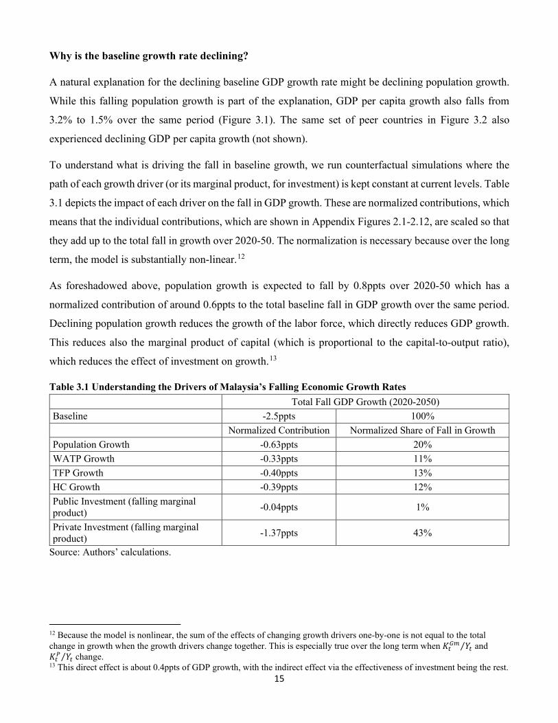
To understand what is driving the fall in baseline growth, we run counterfactual simulations where the
path of each growth driver (or its marginal product, for investment) is kept constant at current levels. Table
3.1 depicts the impact of each driver on the fall in GDP growth. These are normalized contributions, which
means that the individual contributions, which are shown in Appendix Figures 2.1-2.12, are scaled so that
they add up to the total fall in growth over 2020-50. The normalization is necessary because over the long
term, the model is substantially non-linear.12
As foreshadowed above, population growth is expected to fall by 0.8ppts over 2020-50 which has a
normalized contribution of around 0.6ppts to the total baseline fall in GDP growth over the same period.
Declining population growth reduces the growth of the labor force, which directly reduces GDP growth.
This reduces also the marginal product of capital (which is proportional to the capital-to-output ratio),
which reduces the effect of investment on growth.13
Table 3.1 Understanding the Drivers of Malaysia’s Falling Economic Growth Rates Total Fall GDP Growth (2020-2050) Baseline -2.5ppts 100% Normalized Contribution Normalized Share of Fall in Growth Population Growth -0.63ppts 20% WATP Growth -0.33ppts 11% TFP Growth -0.40ppts 13% HC Growth -0.39ppts 12% Public Investment (falling marginal product) -0.04ppts 1%
12 Because the model is nonlinear, the sum of the effects of changing growth drivers one-by-one is not equal to the total change in growth when the growth drivers change together. This is especially true over the long term when 𝐾𝐾𝑡𝑡𝐺𝐺𝐺𝐺 𝑌𝑌𝑡𝑡⁄ and 𝐾𝐾𝑡𝑡𝑃𝑃 𝑌𝑌𝑡𝑡⁄ change. 13 This direct effect is about 0.4ppts of GDP growth, with the indirect effect via the effectiveness of investment being the rest.
16
Declining population growth affects GDP growth and GDP per capita growth differently (in contrast, other
growth drivers have the same effect on GDPPC and GDP growth).14 Falling population growth actually
raises per capita GDP growth: a 1ppts fall in population growth rate reduces the denominator (“per capita”)
by 1ppt, but reduces GDP growth by less than 1 percentage point. In the baseline, GDPPC growth falls by
1.66% in the baseline, but only 1.88% with constant population growth (Appendix Figures 2.1-2.2).
The falling working age-to-total population ratio (WATP ratio) reduces GDP and per capita GDP growth
in the mid-2020s and also late 2040s (Appendix Figures 2.3-2.4). The growth rate of the WATP falls by
0.6ppts by the end of the simulation period, resulting in a contribution of 0.33ppts to the overall fall in
GDP growth over 2020-50.
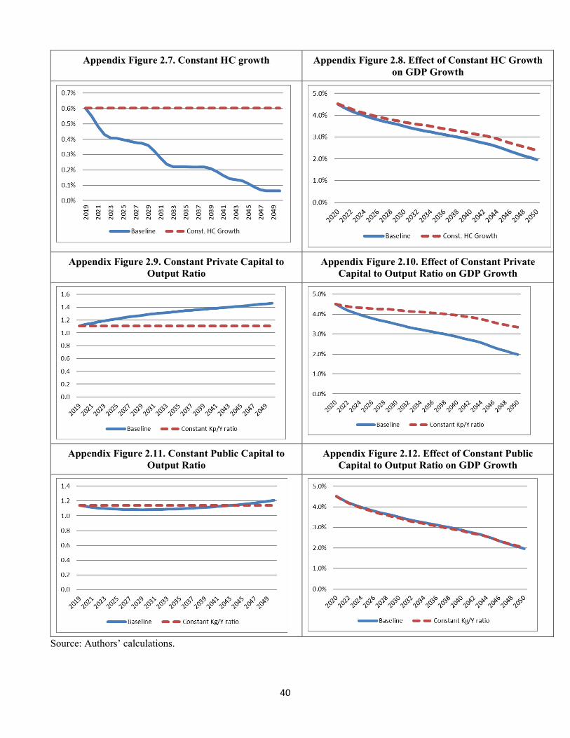
Falling TFP growth and HC growth over 2020-50 both account for around 0.4ppts of the fall in the GDP
growth over 2020-50. The median TFP growth rate over 1985-2014 is 0.9% (the value for the
counterfactual), and the baseline TFP growth rate is expected to decrease from 0.9% to 0.6% over the next
three decades (Figure 2.2B above). Human capital growth falls from 0.6% (the value in the counterfactual)
to 0.1% in the baseline, a 0.5ppts decline (Figure 2.3 above). While this decline in human capital growth
is larger than that of TFP, GDP growth rates are also less sensitive to human capital, resulting in similar
contributions (Appendix Figures 2.5-2.8).
Overall, the declining effectiveness of private investment makes the largest contribution to falling GDP
growth in the baseline (1.4ppts, or 40% of the total). In contrast, changing public investment effectiveness
makes little contribution. Investment rates (public and private) are constant in the baseline, but they can
still contribute to declining growth through changing marginal products. The marginal product of private
capital is currently very high, reflecting low rates of private investment after 2000 and solid historical
growth rates. As private investment is now higher, and growth is slower, the marginal productivity of
private investment is expected to fall through 2050 back to more normal levels.
In our model, the initial private capital-to-output ratio, 𝐾𝐾𝑃𝑃/𝑌𝑌 is relatively low at 1.14 (about the same as
the public capital-to-output ratio 𝐾𝐾𝐺𝐺𝐺𝐺/𝑌𝑌 of 1.11), thus allowing for a much higher marginal product of
private capital. However, with high 𝐼𝐼𝑃𝑃/𝑌𝑌 at a constant 18 percent, 𝐾𝐾𝑃𝑃/𝑌𝑌 also increases faster than 𝐾𝐾𝐺𝐺/𝑌𝑌
(which increases only slightly, due to a public investment share-to-GDP of 6%). As such in the baseline
the marginal product of private capital shows a larger decline, and the GDP growth effect of 𝐼𝐼𝑃𝑃/𝑌𝑌 falls
more noticeably over time.
14 Note however, that the normalized contributions of the other growth drivers will be different for GDP and GDPPC growth.
17
4. Scenario analysis (analysis of shocks to each growth driver)
In this section, we study the impact on growth from shocks to investment, human capital growth, TFP
growth, and FLFP. These are based on, or with reference to, 25th, 50th, and 75th percentiles among high-
income countries (“aspirational goals”). Weak reform scenarios for some factors will be above the
baseline. Additionally, we include a short box on the impact of rebalancing between public and private
Box Article 1. Republic of Korea’s Economic Growth Experience
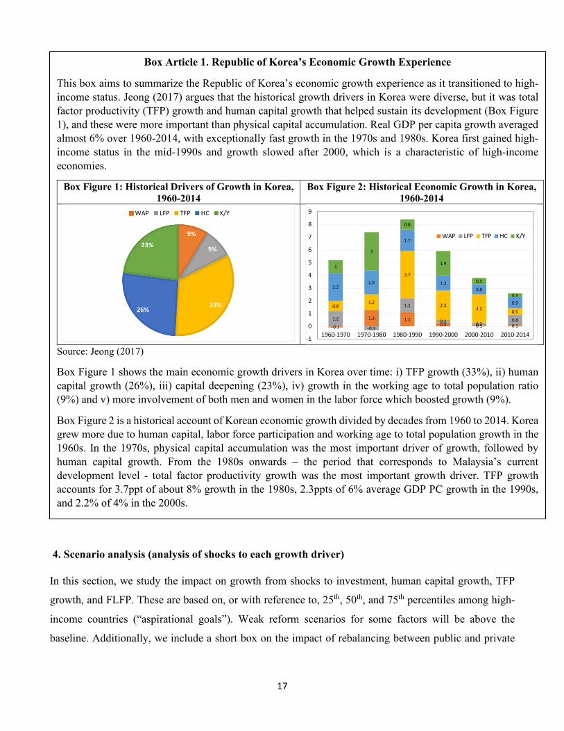
This box aims to summarize the Republic of Korea’s economic growth experience as it transitioned to high-income status. Jeong (2017) argues that the historical growth drivers in Korea were diverse, but it was total factor productivity (TFP) growth and human capital growth that helped sustain its development (Box Figure 1), and these were more important than physical capital accumulation. Real GDP per capita growth averaged almost 6% over 1960-2014, with exceptionally fast growth in the 1970s and 1980s. Korea first gained high-income status in the mid-1990s and growth slowed after 2000, which is a characteristic of high-income economies.
Box Figure 1: Historical Drivers of Growth in Korea, 1960-2014
Box Figure 2: Historical Economic Growth in Korea, 1960-2014
Source: Jeong (2017)
Box Figure 1 shows the main economic growth drivers in Korea over time: i) TFP growth (33%), ii) human capital growth (26%), iii) capital deepening (23%), iv) growth in the working age to total population ratio (9%) and v) more involvement of both men and women in the labor force which boosted growth (9%).
Box Figure 2 is a historical account of Korean economic growth divided by decades from 1960 to 2014. Korea grew more due to human capital, labor force participation and working age to total population growth in the 1960s. In the 1970s, physical capital accumulation was the most important driver of growth, followed by human capital growth. From the 1980s onwards – the period that corresponds to Malaysia’s current development level - total factor productivity growth was the most important growth driver. TFP growth accounts for 3.7ppt of about 8% growth in the 1980s, 2.3ppts of 6% average GDP PC growth in the 1990s, and 2.2% of 4% in the 2000s.
investment (unchanged total investment), when discussing investment shocks to better understand their
relative effects.
4.1 Public and Private Investment Scenarios
4.1.1 Shocks to Public Investment
We consider two alternative public investment scenarios: a 1ppt GDP increase in public investment
(strong reform), and a 1ppt GDP fall in public investment (weak reform). The +1ppt shock, which could
reflect strong revenue mobilization reforms amid faster fiscal consolidation than the baseline, brings 𝐼𝐼𝐺𝐺/𝑌𝑌
to the 90th percentile of the high-income country distribution. The -1ppt shock could reflect faster fiscal
consolidation than the baseline, but with poor revenue mobilization reforms, it would take public
investment as a share of GDP to the 75th percentile.
When we shock the public investment-to-GDP ratio by increasing it from 6% to 7%, GDP growth is
boosted by approximately +0.15ppts over 2021-2030 and approximately +0.10 over 2031-2050. A roughly
symmetric effect on growth, but in the opposite direction, occurs with a decrease in public-investment-to-
GDP from 6% to 5%. Figure 4.1 Panel A illustrates the shocks to 𝐼𝐼𝐺𝐺/𝑌𝑌 comprising strong reform (+1ppt)
and weak reform (-1ppt) scenarios; and graph B, the effects on GDP growth vis-à-vis the baseline. 𝐼𝐼𝑃𝑃/𝑌𝑌
is unchanged from the baseline in these simulations.
Figure 4.1. Shocks to 𝑰𝑰𝑮𝑮/𝒀𝒀 - Impact on GDP Growth A. Public Investment (% of GDP) B. Real GDP Growth
(Difference vis-à-vis Baseline)
19
4.1.2 Shocks to Private Investment
We consider larger shocks than we did for 𝐼𝐼𝐺𝐺/𝑌𝑌, as 𝐼𝐼𝑃𝑃/𝑌𝑌 is higher and varies more across high-income
countries. The +2ppts shock, which we assume occurs as the government delivers reforms that strengthen
the ecosystem for private investment and promotes a rebalancing of investment, brings 𝐼𝐼𝑃𝑃/𝑌𝑌 to the 75th
percentile of the high-income country distribution while the -2ppts shock, reflecting insufficient reforms
amid fiscal consolidation, takes it to the 25th percentile and is also approximately Malaysia’s average over
2010-2018.
When we shock the private investment-to-GDP ratio by increasing it from 18% to 20%, GDP growth is
boosted by approximately +0.36ppts over 2021-2030. But the growth effect falls off sharply – by about
two-thirds to +0.11ppts over 2031-2050. A decrease in private investment-to-GDP from 18% to 16%
reduces GDP growth by -0.39ppts over 2021-2030 and -0.13ppts over 2031-2050. Graph A of Figure 4.2
illustrates the shocks associated with strong reform and weak reform respectively to 𝐼𝐼𝑃𝑃/𝑌𝑌, comprising +/-
2ppts, and graph B the effects on GDP growth vis-à-vis the baseline. 𝐼𝐼𝐺𝐺/𝑌𝑌 is unchanged from the baseline
in these simulations.
Figure 4.2. Shocks to 𝑰𝑰𝑷𝑷/𝒀𝒀 - Impact on GDP Growth A. Private Investment (% of GDP) B. Real GDP Growth
(Difference vis-à-vis Baseline)
20
4.2 Total Factor Productivity Growth
We model three TFP scenarios with different levels of reform by benchmarking Malaysia against high-
income countries. The simulations include a weak reform scenario which targets a low value over a long
period, a strong reform scenario which targets a high value over a short period, and a moderate reform
scenario in the middle. We assume each subcomponent index for innovation, education, market efficiency,
infrastructure, and institutions, which are identified as main determinants of TFP based on a literature
review (Kim and Loayza 2019), increase linearly to the 25th, 50th, and 75th percentiles among high-income
countries for the scenarios of weak, moderate, and strong reforms, respectively. The number of years to
reach the target is 75th (long), 50th, and 25th (short) percentile, respectively, in the distribution of years
that the high-income countries took from the Malaysia’s current level (in 2018) to the target. For example,
for the strong reform scenario for education, there are 5 high-income countries which achieved the target
Box Article 2. Rebalancing Components while keeping 𝐈𝐈 𝐘𝐘⁄ unchanged - A Comparison of the effects of 𝐈𝐈𝐆𝐆/𝐘𝐘 and 𝐈𝐈𝐏𝐏/𝐘𝐘 on GDP Growth
We consider two scenarios, in which total 𝐼𝐼 𝑌𝑌⁄ remains unchanged from the baseline at 24 percent. In the first scenario, we increase 𝐼𝐼𝐺𝐺/𝑌𝑌 by 1ppt to 7 percent and reduce 𝐼𝐼𝑃𝑃/𝑌𝑌 to 17 percent from 2020. There is an initial decline in GDP growth vis-à-vis the baseline (line with marker in graph A of Box Figure 3) given the loss of private investment impact at a high 𝑀𝑀𝑀𝑀𝐾𝐾𝑃𝑃 but the differential turns positive by 2029 and remains so thereafter because 𝐾𝐾𝑃𝑃/𝑌𝑌 rises more slowly compared to the baseline and 𝑀𝑀𝑀𝑀𝐾𝐾𝑃𝑃 is therefore higher (line with marker in graph B of Box Figure 3).
In the second scenario, we reduce 𝐼𝐼𝐺𝐺/𝑌𝑌 by 1ppt to 5 percent and increase 𝐼𝐼𝑃𝑃/𝑌𝑌 to 19 percent from 2020. In contrast to the first scenario, there is an initial increase in GDP growth vis-à-vis the baseline, but the differential turns negative by 2027 (dotted lie in graph A of Box Figure 3), as 𝐾𝐾𝑃𝑃/𝑌𝑌 rises more quickly compared to the baseline and 𝑀𝑀𝑀𝑀𝐾𝐾𝑃𝑃 declines faster (dotted line in graph B of Box Figure 3).
Box Figure 3. Rebalancing Investment Components – Impact on GDP Growth
24.79 52.07 85.26 60.20 69.45 Scenario 1. Weak reform Target value 21.03 60.28 71.66 60.47 72.99 Country - Spain - Portugal Slovakia Years to target - a 8 - b 1 16 Scenario 2. Moderate reform Target value 40.24 71.49 86.89 68.68 82.22 Country France Netherlands Italy Finland France Years to target 9 21 2 13 19 c Scenario 3. Strong reform Target value 59.46 77.53 90.98 73.93 91.70 Country Denmark Sweden Germany Switzerland Germany Years to target 10 20 4 16 d 39 e a, b The subcomponent indexes are assumed to increase over the next 3 decades with Malaysia’s historical trend of the last 10 years (2009-2018). c, e All high-income countries achieved Malaysia’s current level before 1985, the initial year in our database. We used the path of Japan of which the institutions index is the closest (74.01) in 1985 to the current Malaysia’s level (69.45). The institutions index of Japan is assumed to linearly increase in 2019 and onwards with the average annual change of the last 10 years (2009-2018). d All high-income countries achieved Malaysia’s current level before 1985, the initial year in our database. We use the path of Slovenia of which the infrastructure index is the closest (62.62) in 1985 to the current Malaysia’s level (60.20). Note 1. All indexes range from 1, the worst performance, to 100, the best. Note 2. See Appendix 1: LTGM-TFP or Kim and Loayza (2019) for more details on the construction of the determinant indexes.
Only in the strong reform scenario are the growth rates of TFP, GDP, and GDP per capita expected to
exceed those of the business-as-usual baseline. Figure 4.3 shows the path of the TFP determinant index
under the scenarios of weak, moderate, and strong reforms and Figures 4.4-4.6 show the results of the
simulations for the growth of TFP, total GDP, and GDP per capita (respectively). In the weak-reform
22
scenario, the growth rates are lower than those of the business-as-usual baseline. The moderate reform-
reform scenario leads to growth rates very similar to the baseline. Only with the strong-reform scenario,
the growth rates of TFP, total GDP, and GDP per capita are expected to be higher than those of the
baseline.
Figure 4.3-4.6. Simulated paths of the TFP overall determinant index and growth rates of TFP, GDP, and GDP per capita under the scenarios of weak, moderate, and strong reforms
Figure 4.3. TFP Overall Determinant Index Figure 4.4. TFP Growth
Figure 4.5. GDP PC Growth Figure 4.6. GDP Growth
Source: Authors’ calculations.
The key message of the simulations is that the improvement of the TFP overall determinant index needs
to be large and fast enough to maintain or accelerate TFP growth. In our econometric model for the LTGM-
TFP extension, the change in TFP growth rate depends on changes in TFP determinant subcomponent
indexes of innovation, education, market efficiency, infrastructure, and institutions, as well as the initial
level of TFP. A larger projected change in TFP growth rate occurs with larger proportional increases in
23
the TFP determinant subcomponent indexes and lower initial levels of TFP (see Kim and Loayza 2019).
In Malaysia’s case, the current TFP overall determinant index is higher than in other developing countries
on average; increasing it further is harder than in other countries with lower levels of the overall index.
Also, Malaysia’s current level of TFP is moderately high as compared to other developing countries. For
these reasons, achieving higher TFP growth in Malaysia is more difficult than in the past and in
comparison to many other developing countries. Only with the scenario of strong reform, the growth rates
of TFP, GDP, and GDP per capita are expected to be higher than those of the business-as-usual baseline.
4.3 Human Capital Growth
This subsection models shocks to the quantity of education, quality of education, and health components
(adult survival rates and children under 5 years of age who are not stunted) to the 25th, 50th, and 75th
percentiles of high-income economies. The distribution of those four components are explored in Figure
4.7-4.10 below and it can be observed that Malaysia is behind other high-income economies in all four
areas. We perform two sets of simulations: first by shocking all the components together to the different
high-income percentiles, and second by shocking each HC component to the high-income country median
one-at-a-time – to investigate the quantitative importance of each component.
By shocking the components of quality and quantity of education and health components of human capital
to the 25th, 50th, and 75th percentiles of high-income economies, GDP growth is boosted by roughly
0.10ppts, 0.30ppts, and 0.40ppts on average during the 2020-2050 period (Figures 4.11-4.12). The
dynamics are also important. This immediate policy change causes no change in the growth rates of human
capital or GDP until the mid-late 2020s, which is when the oldest children who were affected by the policy
change start to join the labor force. Even then, the effects are small as the oldest cohort of children spent
the majority of their education under the old regime, and so only enjoy a fraction of the benefits. It takes
until almost 2040 for the reforms to have their full effect: when today’s toddlers – who received the full
benefit of the reforms – start to join the labor market.
24
Figure 4.7. Expected Years of Schooling Figure 4.8. Malaysia’s Quality of Education
Figure 4.12. GDP Growth due to Human Capital Reforms
Sources: Figure 4.7-4.10 from Human Capital Index; Figure 4.11, 4.12 from authors’ calculations.
To understand the effect of each human capital component, we shock each component to the 50th percentile
of the HI distribution one-by-one (Figure 4.13). On average over 2020-50, a higher quality of education
25
boosts GDP growth by 0.14ppts, an increase in the years of schooling boosts growth by 0.10ppts,
increasing the adult survival rate boosts growth by 0.02ppts, and lowering stunting rates among children
under 5 boosts growth by 0.02ppts (Figure 4.14). Quantity and quality of education provide the biggest
boost to economic growth in long run.15 In numerical terms, the high-income-median targets are 13.4
expected years of schooling, 83% quality of education, adult survival rate of 93% and the fraction of
children not stunted under 5 of 93%. These improvements in human capital growth components prevent
the decline in human capital growth in the baseline and instead boost it from 0.6% to 0.7% by 2050
(instead of falling to 0.1%).16
Figure 4.13: Malaysia’s Human Capital Growth – Disaggregation by Components
Figure 4.14: Malaysia’s GDP Growth due to Human Capital Growth by Component
Source: Authors’ calculations.
4.4. Female Labor Force Participation
An increase in female labor force participation (FLFP) to the 25th, 50th and 75th percentiles of high-income
economies boosts average GDP growth over 2020-50 by 0.14ppts, 0.31ppts, and 0.36ppts, respectively,
relative to the business-as-usual baseline with unchanged FLFP. The FLFP rate in Malaysia is 55% as of
2018, which is low in comparison to its regional peers (see Figure 1.11) and also to its high-income peers
(see Figure 4.15). We simulate increases from the current FLFP of 55% to the 25th (weak reform), 50th
(moderate reform), and 75th (strong reform) percentiles of FLFP of high-income economies, for which the
number of years to reach the target is 75th (long), 50th, and 25th (short) percentiles, respectively, in the
distribution of years that the high-income countries took from the Malaysia’s current level (in 2018) to
15 However, it should be noted that the health components improve the standards of living of Malaysians as a whole and by being healthy, they are able to learn and improve their educational attainment and also be healthier workers. The LTGM-HC does not include the indirect effect of health on growth via high education. 16 This simulation is similar to that in the June 2019 Malaysian Macroeconomic Monitor, the differences being that (i) baseline has changed slightly to include a downward trend in TFP growth and (ii) quantity of education is also shocked.
26
the target.17 We find that these increases in FLFP boost GDP growth by about 0.15ppts, 0.30ppts, and 0.40ppts
over 2020-50, respectively, relative to the business-us-usual baseline with unchanged FLFP (Figures 4.17-4.18).
Figure 4.15. FLFP Distribution of High-Income Economies Figure 4.16. FLFP Simulations
Figure 4.17. Malaysia’s GDP PC Growth due to increases in FLFP
Figure 4.18. Malaysia’s GDP Growth due to increases in FLFP
Source: Authors’ calculations.
5. Combined Shocks to Generate Weak, Moderate and Strong Reform Growth Paths
Malaysia is heading to high income status in the next decade and the business-as-usual baseline suggests
that GDP growth will more than halve over the 2020-50 period. More importantly for living standards,
GDP per capita growth is also expected to halve over the same period. While this is common among
17 For example, in the weak reform, the target FLFP is 62% which is the 25th percentile among HI countries and of Croatia in 2018. For calculating a target duration to reach 62%, we identified 8 high-income countries which show the path of FLFP from Malaysia’s current level to the target (55% to 62%) within the time period of our database (1990-2018). Then the target duration was calculated at 27 years, which is the 75th percentile in the years the 8 countries took to reach from 55% to 62%. With the same approach, the moderate reform scenario targets 69% (Spain in 2018) over 23 years, and the strong-reform scenario, 74% (Netherlands in 2018) over 27 years17 (Figure 4.16).
27
economies making the transition to high income status, slowing growth can – at least partially – be offset
by pro-growth reforms.
In this section, we simulate the combined growth effects of a package of reforms affecting human capital
growth, TFP growth, female labor force participation rate and/or investment. The components of the
package of reforms are the same as those discussed individually in Section 4; here we combine their
effects. The results are shown in Figures 5.1 and 5.2.
Figure 5.1. Malaysia’s GDP PC Growth due to Reforms
Figure 5.2. Malaysia’s GDP Growth due to Reforms
Source: Authors’ calculations.
In the weak reform scenario, based on increasing the growth determinants to the 25th percentile of high-
income countries (as above), growth is around 0.6ppts lower than the baseline in the early 2020s, but
converges to the baseline by around 2040. The initial fall in growth is due mostly to lower investment
rates: a fall in public investment (relative to the baseline) of around 1ppt of GDP, and a fall in private
investment (relative to the baseline) of around 2ppts of GDP. These have an immediate negative effect on
growth – especially the cut in private investment – given that the marginal product of private capital is
initially very high. Slower TFP growth, which is lower in the weak reform scenario than the baseline, also
makes a small negative contribution. The catchup in the medium term is driven mostly by human capital,
where even weak-reform boosts growth relative to business as usual– albeit with a lag. The human capital
lag is driven by the time it takes better educated, healthier children to grow up to become more productive
workers.
In the moderate reform scenario, growth is higher at all horizons and averages 0.6ppts higher over 2020-
50. Public and private investment stays constant in the moderate reform scenarios (as in the baseline),
which is why the change in growth around 2020 is small. In addition, the moderate-reform TFP growth is
very similar to baseline, and so makes little contribution in either direction. Consequently, the boost to
28
growth in the first 10-15 years in the moderate reform package is mostly due to higher FLFP. After that,
the boost to growth increases further as today’s children, with higher human capital, start to join the labor
force around 2035-40. While GDP growth does still decline, it does so at a reduced rate and the downward
trend in GDP per capita growth is checked until 2040.
Finally, in the strong reform scenario, based on growth determinants at the 75th percentile of high-income
countries, growth is about around 1.5ppts higher than the baseline over 2020-2050. The decline in GDP
growth (relative to 2020) is delayed until 2042, and GDP per capita growth is higher than its 2020 rate at
almost all horizons. Growth increases initially to 5.5%, mostly based on higher private (and public)
investment. Higher TFP growth and FLFP boost GDP growth as well, joined by human capital after around
2035-40. It should be noted, however, that such a path represents the most optimistic path for growth and
reforms.
6. Conclusions
The main findings of the paper can be summarized as follows. With the business-as-usual baseline, the
GDP growth rate is expected to fall from 4.5% to 2.0% over the next 30 years (2020-2050), which covers
the period of the country’s transition to high-income status and beyond. This decline is partly due to
demographics, but the other main causes are 1) a smaller contribution from private investment as private
capital accumulates and its marginal product declines, and 2) the gradual moderation in the growth rates
of TFP and human capital, for which continuous improvements at a high growth rate become more
difficult as their levels increase.
Under the scenario of weak reform, the GDP growth rate is expected to decrease from 4.5% to 2.0% over
the next 30 years, which is similar to the result of the baseline. The impact is minimal compared to the
baseline because the expected paths of growth drivers under this scenario are similar to those of the
baseline. Under the scenario of moderate reform, the GDP growth rate is expected to decrease from 4.5%
to 2.9%, which is around 1.5 times the GDP growth rate of the baseline in 2050. Under the scenario of
strong reform, GDP growth rate is expected to decrease from 4.5% to 3.6%, which is around 1.8 times
higher than that under the baseline in 2050. Higher overall investment-to-GDP due to a better fiscal
position and private investment ecosystem supports growth in the short-to-medium term but its weakening
incremental effect must be offset by other factors. The strong reform scenario clearly illustrates how the
stronger contributions emanating from growth in human capital (0.28ppts growth increase with respect to
the baseline, or 39% of the growth differential), TFP (0.02ppts or 30%), and female labor force
29
participation rate (0.30ppts or 24%) can, to some extent, mitigate the diminishing returns to physical
capital accumulation over the long term (7% of the growth differential vis-à-vis the baseline).
The policy implications are derived from these results. Strong reforms are required to grow beyond what
is expected based on historical trends, especially for human capital (the quantity and quality of schooling,
and health), female labor force participation, and TFP. If Malaysia stays at the current level of educational
quality and health (similar to the 25th percentile of high-income countries), human capital will not
contribute much to economic growth. Improving human capital requires more focus on enhancing learning
outcomes, improving child nutrition, and providing adequate protection through social welfare programs
(World Bank 2018). Current female labor force participation is lower than the 25th percentile of high-
income countries, which is the benchmark of the weak-reform scenario. Increasing it requires reducing or
eliminating barriers to economic opportunities for women through legal reforms, introducing more
economic and societal support for parents, and addressing gender norms and attitudes that perpetuate
disparities (World Bank 2019). Strong reforms to increase TFP growth require efforts from diverse
stakeholders. Our study shows that the gap between Malaysia’s current level (in 2018) and a target
corresponding to the 75th percentile of high-income countries is relatively small for market efficiency but
becomes increasingly wider for innovation, infrastructure, education, and institutions. Some of them, such
as education and institutions, are expected to require two decades or more to improve to the target level
of high-income economies. As these determinants are intercorrelated, sustainable collaboration and
cooperation among the government, private sector, and civil society will be necessary.
30
References
Devadas, S. and S.M. Pennings. 2019. Assessing the Effect of Public Capital on Growth: An Extension
of the World Bank Long-Term Growth Model. Journal of Infrastructure, Policy and Development 3(1):
22-55.
International Monetary Fund. 2019. Malaysia: Staff Report for the 2019 Article IV Consultation.
Washington: International Monetary Fund.
Jeong, H. 2017. Korea's growth experience and the long-term growth model. Policy Research Working
Paper WPS8240. Washington, D.C.: World Bank Group.
Kim, Y.E. and N.V. Loayza. 2019. Productivity Growth: Patterns and Determinants across the World.
Policy Research working paper WPS 8852. Washington, D.C.: World Bank Group.
Kowalski, P., M. Büge, M. Sztajerowska and M. Egeland. 2013. State-Owned Enterprises: Trade Effects
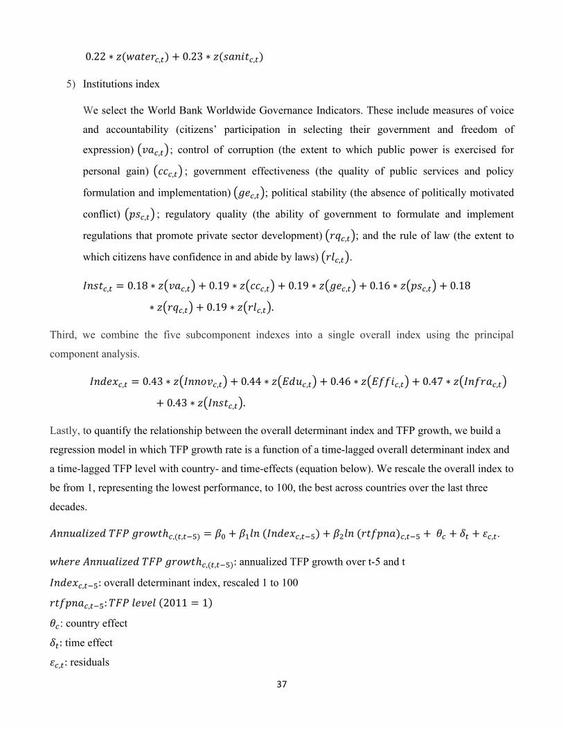
𝑚𝑚ℎ𝐻𝐻𝑎𝑎𝐻𝐻 𝐴𝐴𝑜𝑜𝑜𝑜𝑒𝑒𝐻𝐻𝑜𝑜𝑜𝑜𝑧𝑧𝐻𝐻𝑠𝑠 𝑇𝑇𝑇𝑇𝑀𝑀 𝑔𝑔𝑎𝑎𝑜𝑜𝑚𝑚𝐻𝐻ℎ𝑌𝑌,(𝑡𝑡,𝑡𝑡−5): annualized TFP growth over t-5 and t
𝐼𝐼𝑜𝑜𝑠𝑠𝐻𝐻𝑥𝑥𝑌𝑌,𝑡𝑡−5: overall determinant index, rescaled 1 to 100
𝑎𝑎𝐻𝐻𝑓𝑓𝑝𝑝𝑜𝑜𝐻𝐻𝑌𝑌,𝑡𝑡−5:𝑇𝑇𝑇𝑇𝑀𝑀 𝑜𝑜𝐻𝐻𝑣𝑣𝐻𝐻𝑜𝑜 (2011 = 1)
𝜃𝜃𝑌𝑌: country effect
𝛿𝛿𝑡𝑡: time effect
𝜀𝜀𝑌𝑌,𝑡𝑡: residuals
38
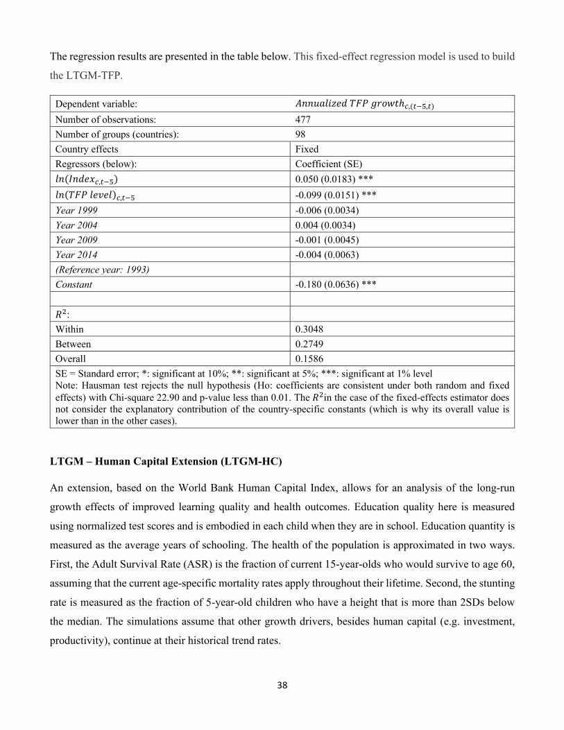
The regression results are presented in the table below. This fixed-effect regression model is used to build
the LTGM-TFP.
Dependent variable: 𝐴𝐴𝑜𝑜𝑜𝑜𝑒𝑒𝐻𝐻𝑜𝑜𝑜𝑜𝑧𝑧𝐻𝐻𝑠𝑠 𝑇𝑇𝑇𝑇𝑀𝑀 𝑔𝑔𝑎𝑎𝑜𝑜𝑚𝑚𝐻𝐻ℎ𝑌𝑌,(𝑡𝑡−5,𝑡𝑡) Number of observations: 477 Number of groups (countries): 98 Country effects Fixed Regressors (below): Coefficient (SE) 𝑜𝑜𝑜𝑜(𝐼𝐼𝑜𝑜𝑠𝑠𝐻𝐻𝑥𝑥𝑌𝑌,𝑡𝑡−5) 0.050 (0.0183) *** 𝑜𝑜𝑜𝑜(𝑇𝑇𝑇𝑇𝑀𝑀 𝑜𝑜𝐻𝐻𝑣𝑣𝐻𝐻𝑜𝑜)𝑌𝑌,𝑡𝑡−5 -0.099 (0.0151) *** Year 1999 -0.006 (0.0034) Year 2004 0.004 (0.0034) Year 2009 -0.001 (0.0045) Year 2014 -0.004 (0.0063) (Reference year: 1993) Constant -0.180 (0.0636) *** 𝑅𝑅2: Within 0.3048 Between 0.2749 Overall 0.1586 SE = Standard error; *: significant at 10%; **: significant at 5%; ***: significant at 1% level Note: Hausman test rejects the null hypothesis (Ho: coefficients are consistent under both random and fixed effects) with Chi-square 22.90 and p-value less than 0.01. The 𝑅𝑅2in the case of the fixed-effects estimator does not consider the explanatory contribution of the country-specific constants (which is why its overall value is lower than in the other cases).
LTGM – Human Capital Extension (LTGM-HC)
An extension, based on the World Bank Human Capital Index, allows for an analysis of the long-run
growth effects of improved learning quality and health outcomes. Education quality here is measured
using normalized test scores and is embodied in each child when they are in school. Education quantity is
measured as the average years of schooling. The health of the population is approximated in two ways.
First, the Adult Survival Rate (ASR) is the fraction of current 15-year-olds who would survive to age 60,
assuming that the current age-specific mortality rates apply throughout their lifetime. Second, the stunting
rate is measured as the fraction of 5-year-old children who have a height that is more than 2SDs below
the median. The simulations assume that other growth drivers, besides human capital (e.g. investment,
productivity), continue at their historical trend rates.
39
Appendix 2. Extra graphs explaining the declining GDP growth in the baseline
Appendix Figure 2.1. Constant Population Growth counterfactual
Appendix Figure 2.2. Graph Effect of Population Growth on GDP Growth
Appendix Figure 2.3. Constant working age to
population Appendix Figure 2.4. Graph Effect of WATP Growth
on GDP Growth
Appendix Figure 2.5. TFP growth: constant rate at the historical median
Appendix Figure 2.6. Effect on GDP growth of the two TFP growth paths: constant rate at the historical
median
40
Appendix Figure 2.7. Constant HC growth Appendix Figure 2.8. Effect of Constant HC Growth on GDP Growth
Appendix Figure 2.9. Constant Private Capital to
Output Ratio Appendix Figure 2.10. Effect of Constant Private
Capital to Output Ratio on GDP Growth
Appendix Figure 2.11. Constant Public Capital to Output Ratio
Appendix Figure 2.12. Effect of Constant Public Capital to Output Ratio on GDP Growth