1 Module 8 Fixed overhead analysis and reporting for control Lectures and handouts by: Shirley Mauger, MBA, HB Comm, CGA Management Accounting Fundamentals 2 Module 8 - Table of Contents 8.1 Overhead rates and standard costing 8.2 Fixed overhead budget and volume variances 8.3 Journal entries to record standard costs and variances 8.4 Computer illustration 8.4-1: Fixed costs in a flexible budget 8.5 Full income statement variance analysis 8.6 Decentralization in organizations 8.7 Segment reporting 8.8 Revenue variance and marketing expense analysis 8.9 Return on investment and residual income 8.10 Balanced scorecard 8.11 Other performance measures 1 N/A 2 3 4 Part Content 3 Module 8 - Table of Contents Review question: Variance analysis and journal entries Review question: Variance analysis, working backwards from data Review question: Segmented statements Review question: Segmented statements, ROI and residual income Review question: Sales and market variances (High low method) Review question: Multiple choice 5 6 7 8 9 10 Part Content
Transcript
1
Module 8
Fixed overhead analysis and
reporting for control
Lectures and handouts by:
Shirley Mauger, MBA, HB Comm, CGA
Management Accounting
Fundamentals
2
Module 8 - Table of Contents
8.1 Overhead rates and standard costing
8.2 Fixed overhead budget and volume variances
8.3 Journal entries to record standard costs and variances
8.4 Computer illustration 8.4-1: Fixed costs in a flexible budget
8.5 Full income statement variance analysis
8.6 Decentralization in organizations
8.7 Segment reporting
8.8 Revenue variance and marketing expense analysis
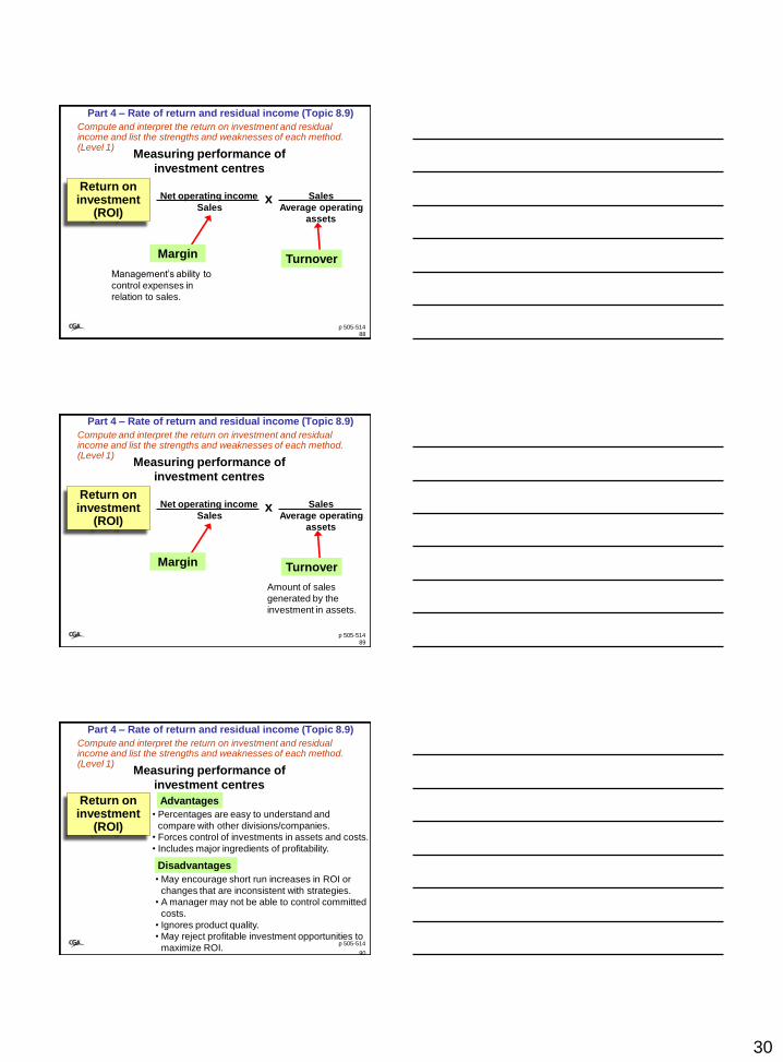
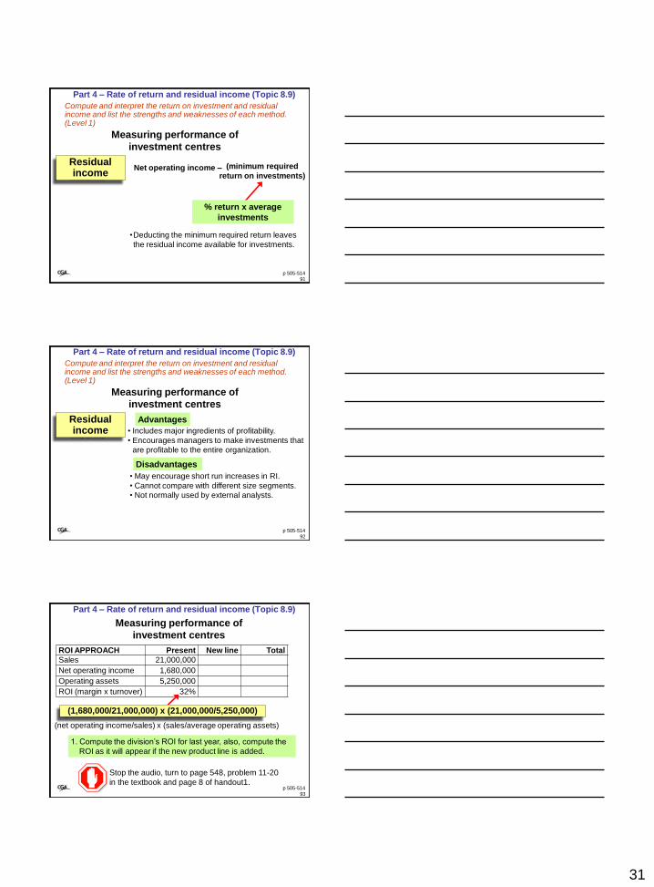
8.9 Return on investment and residual income
8.10 Balanced scorecard
8.11 Other performance measures
1
N/A
2
3
4
Part Content
3
Module 8 - Table of Contents
Review question: Variance analysis and journal entries
Review question: Variance analysis, working backwards from
data
Review question: Segmented statements
Review question: Segmented statements, ROI and residual
income
Review question: Sales and market variances (High low method)
Review question: Multiple choice
5
6
7
8
9
10
Part Content
2
4
Part 1
Overhead rates and standard costing
Fixed overhead budget and volume variances
Journal entries to record standard cost variances
Topics 8.1 - 8.3
MA1 – MODULE 8
Part 1 – Overhead rates and standard costing (Topic 8.1)
Explain the significance of the denominator activity figure in determining the standard cost of a unit of product. (Level 1)
5
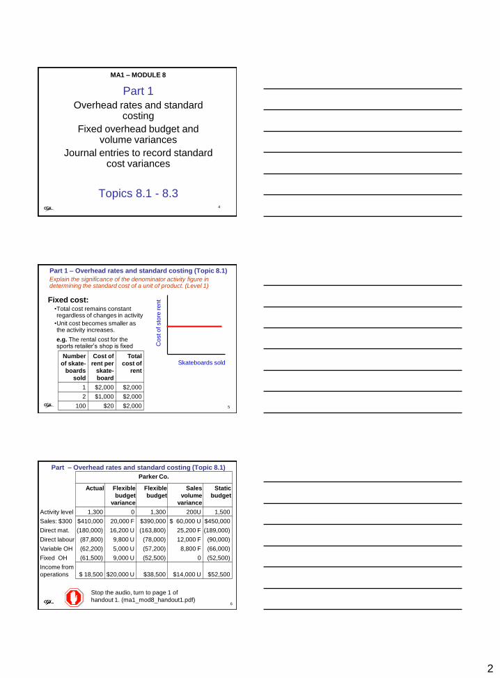
Fixed cost: •Total cost remains constant regardless of changes in activity
•Unit cost becomes smaller as the activity increases.
e.g. The rental cost for the sports retailer’s shop is fixed
Skateboards sold
Co
st o
f sto
re r
en
t
Number
of skate-
boards
sold
Cost of
rent per
skate-
board
Total
cost of
rent
1 $2,000 $2,000
2 $1,000 $2,000
100 $20 $2,000
6
Stop the audio, turn to page 1 of
handout 1. (ma1_mod8_handout1.pdf)
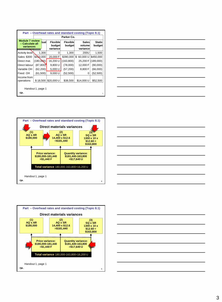
Part – Overhead rates and standard costing (Topic 8.1)
Parker Co.
Actual Flexible
budget
variance
Flexible
budget
Sales
volume
variance
Static
budget
Activity level 1,300 0 1,300 200U 1,500
Sales: $300 $410,000 20,000 F $390,000 $ 60,000 U $450,000
Direct mat. (180,000) 16,200 U (163,800) 25,200 F (189,000)
Direct labour (87,800) 9,800 U (78,000) 12,000 F (90,000)
Variable OH (62,200) 5,000 U (57,200) 8,800 F (66,000)
Fixed OH (61,500) 9,000 U (52,500) 0 (52,500)
Income from
operations $ 18,500 $20,000 U $38,500 $14,000 U $52,500
3
7
Handout 1, page 1
Part – Overhead rates and standard costing (Topic 8.1)
Parker Co.
Actual Flexible
budget
variance
Flexible
budget
Sales
volume
variance
Static
budget
Activity level 1,300 0 1,300 200U 1,500
Sales: $300 $410,000 20,000 F $390,000 $ 60,000 U $450,000
Direct mat. (180,000) 16,200 U (163,800) 25,200 F (189,000)
Direct labour (87,800) 9,800 U (78,000) 12,000 F (90,000)
Variable OH (62,200) 5,000 U (57,200) 8,800 F (66,000)
Fixed OH (61,500) 9,000 U (52,500) 0 (52,500)
Income from
operations $ 18,500 $20,000 U $38,500 $14,000 U $52,500
Module 7 review – Calculate all
variances
8
Part – Overhead rates and standard costing (Topic 8.1)
Quantity variance:$181,440-163,800
=$17,640 U
Price variance:$180,000-181,440
=$1,440 F
Direct materials variances
(1)AQ x AR$180,000
(3)SQ x SR
1300 x 10 x $12.60 = $163,800
Total variance 180,000-163,800=16,200 U
(2)AQ x SR
14,400 x $12.6=$181,440
Handout 1, page 1
9
Part – Overhead rates and standard costing (Topic 8.1)
Quantity variance:$181,440-163,800
=$17,640 U
Price variance:$180,000-181,440
=$1,440 F
Direct materials variances
(1)AQ x AR$180,000
(3)SQ x SR
1300 x 10 x $12.60 = $163,800
Total variance 180,000-163,800=16,200 U
(2)AQ x SR
14,400 x $12.6=$181,440
Handout 1, page 1
4
10
Part – Overhead rates and standard costing (Topic 8.1)
Efficiency variance:$78,000 – 78,000
= 0
Rate variance:$87,800 – 78,000
= $9,800 U
Direct labour variances
(1)AQ x AR$87,800
(3)SQ x SR
1300 x 5 x $12 = $78,000
Total variance 87,800 – 78,000 = $9,800 U
(2)AQ x SR
6500 x $12 = $78,000
Handout 1, page 1
11
Part – Overhead rates and standard costing (Topic 8.1)
Efficiency variance:$57,200 – 57,200
= 0
Spending variance:$62,200 - $57,200
= $5,000 U
Variable overhead variances
(1)AQ x AR$62,200
(3)SQ x SR
5 x 1300 x $8.80 = $57,200
Total variance $62,200 – 57,200 = $5,000 U
(2)AQ x SR
6500 x $8.80 = $57,200
Handout 1, page 1
12
Handout 1, page 1
Part – Overhead rates and standard costing (Topic 8.1)
Parker Co.
Actual Flexible
budget
variance
Flexible
budget
Sales
volume
variance
Static
budget
Activity level 1,300 0 1,300 200U 1,500
Sales: $300 $410,000 20,000 F $390,000 $ 60,000 U $450,000
Direct mat. (180,000) 16,200 U (163,800) 25,200 F (189,000)
Direct labour (87,800) 9,800 U (78,000) 12,000 F (90,000)
Variable OH (62,200) 5,000 U (57,200) 8,800 F (66,000)
Fixed OH (61,500) 9,000 U (52,500) 0 (52,500)
Income from
operations $ 18,500 $20,000 U $38,500 $14,000 U $52,500
Budget and production
volume variances
5
13
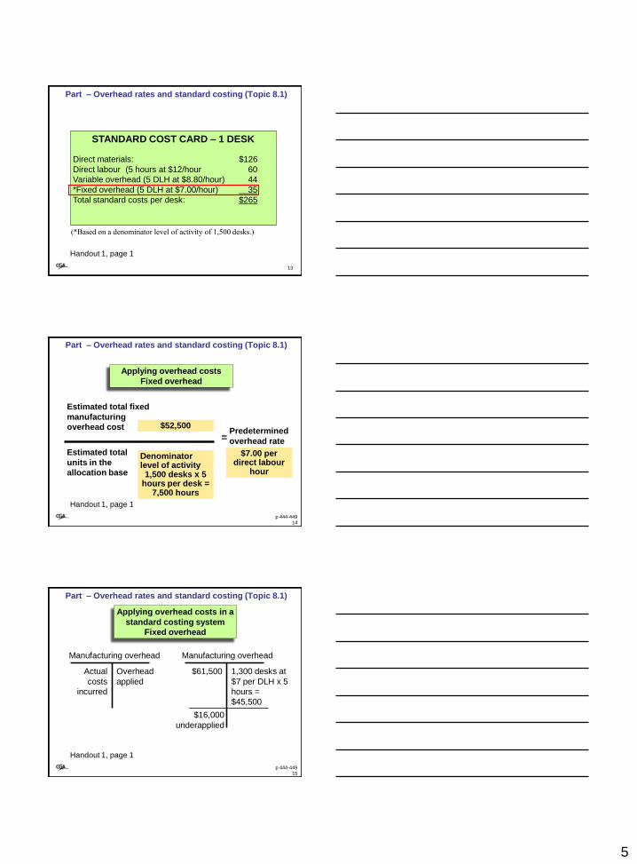
STANDARD COST CARD – 1 DESK
Direct materials: $126
Direct labour (5 hours at $12/hour 60
Variable overhead (5 DLH at $8.80/hour) 44
*Fixed overhead (5 DLH at $7.00/hour) 35
Total standard costs per desk: $265
(*Based on a denominator level of activity of 1,500 desks.)
Part – Overhead rates and standard costing (Topic 8.1)
Handout 1, page 1
Predetermined
overhead rate
Applying overhead costs
Fixed overhead
=
Estimated total fixed
manufacturing
overhead cost
Estimated total
units in the
allocation base
$52,500
Denominator level of activity1,500 desks x 5
hours per desk = 7,500 hours
$7.00 per direct labour
hour
14p 444-449
Part – Overhead rates and standard costing (Topic 8.1)
Handout 1, page 1
Applying overhead costs in a
standard costing system
Fixed overhead
Manufacturing overhead
Actual
costs
incurred
Overhead
applied
Manufacturing overhead
$61,500 1,300 desks at
$7 per DLH x 5
hours =
$45,500
$16,000
underapplied
15
Part – Overhead rates and standard costing (Topic 8.1)
Handout 1, page 1
p 444-449
6
Volume variance:(2)-(3)
Budget variance:(1)-(2)
Fixed overhead variances
(1)Actual cost
$61,500
(3)AU x SQ x SR
Total variance (1)-(3)
(2)BU x SQ x SR
Budgeted units = Denominator level of activity
Part 1 – Fixed overhead budget and volume variances
(Topic 8.2)Compute and properly interpret the fixed overhead budget and volume variances. (Level 1)
16Handout 1, page 1 p 444-449
Volume variance:(2)-(3)
Budget variance:(1)-(2)
Fixed overhead variances
(1)Actual cost
$61,500
(3)AU x SQ x SR
1,300 desks x 5 hours x $7=
$45,500
Total variance $61,500 - $45,500 = $16,000 U
(2)BU x SQ x SR
Budgeted units = Denominator level of activity
17
Part 1 – Fixed overhead budget and volume variances
(Topic 8.2)
Handout 1, page 1 p 444-449
Volume variance:(2)-(3)
Budget variance:(1)-(2)
Fixed overhead variances
(1)Actual cost
$61,500
(3)AU x SQ x SR
1,300 desks x 5 hours x $7=
$45,500
Total variance $61,500 - $45,500 = $16,000 U
(2)BU x SQ x SR
1,500 desks x 5 hours x $7=
$52,500
18
Part 1 – Fixed overhead budget and volume variances
(Topic 8.2)
Handout 1, page 1 p 444-449
7
Volume variance:(2)-(3)
Budget variance:$61,500 - $52,500 =
$9,000 U
Fixed overhead variances
(1)Actual cost
$61,500
(3)AU x SQ x SR
1,300 desks x 5 hours x $7=
$45,500
Total variance $61,500 - $45,500 = $16,000 U
(2)BU x SQ x SR
1,500 desks x 5 hours x $7=
$52,500
More was spent
than planned.
19
Part 1 – Fixed overhead budget and volume variances
(Topic 8.2)
Handout 1, page 1 p 444-449
Volume variance:$52,500 - $45,500 =
$7,000 U
Budget variance:$61,500 - $52,500 =
$9,000 U
Fixed overhead variances
(1)Actual cost
$61,500
(3)AU x SQ x SR
1,300 desks x 5 hours x $7=
$45,500
Total variance $61,500 - $45,500 = $16,000 U
(2)BU x SQ x SR
1,500 desks x 5 hours x $7=
$52,500
200 less units were
produced and sold.
20
Part 1 – Fixed overhead budget and volume variances
(Topic 8.2)
Handout 1, page 1 p 444-449
Part 1 – Journal entries to record standard costs and
variances (Topic 8.3)Prepare journal entries to record standard costs and variances. (Level 2)
Formal entries to record variances:
1. Raw materials purchases
2. Issuing raw materials to production
3. Incurrence of direct labour
4. Variable and fixed overhead (not demonstrated here)
Chapter 10 appendix 10B
21p 462-464
8
Part 1 – Journal entries to record standard costs and
variances (Topic 8.3)Prepare journal entries to record standard costs and variances. (Level 2)
Formal entries to record variances:
1. Raw materials purchases
2. Issuing raw materials to production
3. Incurrence of direct labour
4. Variable and fixed overhead (not demonstrated here)
Chapter 10 appendix 10B
Stop the audio, turn to Problem 10-27 p.477
In the textbook 22p 462-464
Accounts Payable Raw materials
DM price variance
Wages payable
DM quantity variance
Work in progress
DL efficiency varianceDL rate variance
23
Part 1 – Journal entries to record standard costs and
variances (Topic 8.3)
p 462-464
DR Direct materials AQ x SR 8,000 x $6.00
48,000
CR Direct materials price
variance AQ x (SR-AR) 8,000 x (6-5.75)
2,000
CR Accounts Payable AQ x AR 46,000
1. A total of 8,000 kilograms of material were
purchased at a cost of $46,000
24
Part 1 – Journal entries to record standard costs and
variances (Topic 8.3)
p 462-464
9
Accounts Payable Raw materials
46,000
DM price variance
2,000
48,000
Wages payable
DM quantity variance
Work in progress
DL efficiency varianceDL rate variance
25
Part 1 – Journal entries to record standard costs and
variances (Topic 8.3)
p 462-464
2. Issued 6,000 kilograms of materials to production
to produce 3,000 units
DR Work in processSQ x SR 3,000 x 1.5 x $6
27,000
DR Direct materials quantity
variance (AQ-SQ)xSR ( 6,000-(3,000x1.5))x$6
9,000
CR Direct materialsAQ x SR 6,000 x $6
36,000
26
Part 1 – Journal entries to record standard costs and
variances (Topic 8.3)
p 462-464
Accounts Payable Raw materials
46,000
DM price variance
2,000
48,000
Wages payable
DM quantity variance
9,000
36,000
Work in progress
27,000
DL efficiency varianceDL rate variance
27
Part 1 – Journal entries to record standard costs and
variances (Topic 8.3)
p 462-464
10
3. Recorded the direct labour wages for June
DR Work in processSQ x SR 3,000 x .6 x $12
21,600
DR Labour rate variance AQx(AR-SR) (10 x 160 x $12.50-$12)
800
CR Labour efficiency variance(AQ-SQ) x SR ((10x160)-(3,000x.6))x$12
2,400
CR Wages payableAQ x AR 10x160x$12.50
20,000
28
Part 1 – Journal entries to record standard costs and
variances (Topic 8.3)
p 462-464
Accounts Payable Raw materials
46,000
DM price variance
2,000
48,000
Wages payable
DM quantity variance
9,000
36,000
Work in progress
27,000
21,600
20,000
DL efficiency variance
2,400
DL rate variance
800
29
Part 1 – Journal entries to record standard costs and
variances (Topic 8.3)
p 462-464
30
Part 2
Full income statement variance analysis
Decentralization in organizations
Segment reporting
Topics 8.5 - 8.7
MA1 – MODULE 8
11
Part 2 – Full income statement variance analysis (Topic 8.5)
Prepare an income statement incorporating variance analysis. (Level 2)
Part 2 – Full income statement variance analysis (Topic 8.5)
Sales $xxx
Cost of goods sold (standard costs) $xxx
Write off variances
Direct materials price and quantity xxx
Direct labour rate and efficiency xxx
Variable overhead spending and efficiency xxx
Adjusted cost of goods sold xxx
Variable selling and administration xxx xxx
Contribution margin xxx
Fixed manufacturing overhead xxx
Fixed selling and administration xxx
Net income $xxx
Part 2 – Decentralization in organizations (Topic 8.6)
Differentiate between cost centres, profit centres, and investment centres, and explain how performance is measured in each. (Level 2)
Board of directors
CEO
Western
division
Eastern
division
Director of human resources
Consumer
products
Industrial
products
Consumer
products
Industrial
products
DecentralizationDecision making is
spread throughout
the organization.
36p 496-497
13
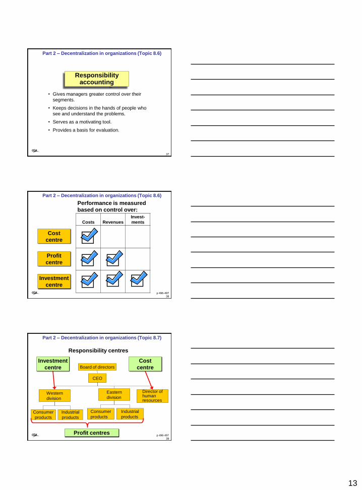
Responsibility accounting
• Gives managers greater control over their
segments.
• Keeps decisions in the hands of people who
see and understand the problems.
• Serves as a motivating tool.
• Provides a basis for evaluation.
Part 2 – Decentralization in organizations (Topic 8.6)
37
Part 2 – Decentralization in organizations (Topic 8.6)
Performance is measured
based on control over:
Investment
centre
Cost
centre
Profit
centre
Costs Revenues
Invest-
ments
38p 496-497
Part 2 – Decentralization in organizations (Topic 8.7)
Board of directors
CEO
Western
division
Eastern
division
Director of human resources
Consumer
products
Industrial
products
Consumer
products
Industrial
products
Responsibility centres
Cost
centre
Profit centres
Investment
centre
39p 496-497
14
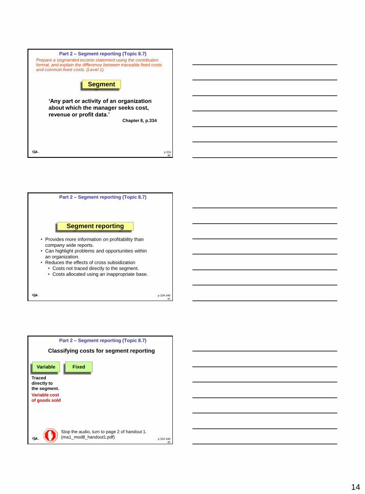
Segment
„Any part or activity of an organization
about which the manager seeks cost,
revenue or profit data.‟Chapter 8, p.334
Part 2 – Segment reporting (Topic 8.7)
40p 334
Prepare a segmented income statement using the contribution format, and explain the difference between traceable fixed costs and common fixed costs. (Level 1)
Part 2 – Segment reporting (Topic 8.7)
Segment reporting
• Provides more information on profitability than
company wide reports.
• Can highlight problems and opportunities within
an organization.
• Reduces the effects of cross subsidization
• Costs not traced directly to the segment.
• Costs allocated using an inappropriate base.
41p 334-340
Part 2 – Segment reporting (Topic 8.7)
Classifying costs for segment reporting
Traced
directly to
the segment.
Variable Fixed
Variable cost
of goods sold
Stop the audio, turn to page 2 of handout 1.
(ma1_mod8_handout1.pdf)42
p 334-340
15
Part 2 – Segment reporting (Topic 8.7)
Classifying costs for segment reporting
Traced
directly to
the segment.
Variable Fixed
Traceable Common
Supports more
than one segment
and not traceable
to any segment.
• Salary of the CEO
• Shared equipment
costs
Directly supports
the segment. Can
become common
as segments are
further divided.• Salary of the
segment manager.
43p 334-340
Part 2 – Segment reporting (Topic 8.7)
Classifying costs for segment reporting
Traced
directly to
the segment.
Variable Fixed
Common
Supports more
than one segment
and not traceable
to any segment.
Can be controlled
by the segment
manager.
CanNOT be
controlled by the
segment manager.
• Advertising for
that segment
• Depreciation of
plant facilities
Traceable
Discretionary Committed
44p 334-340
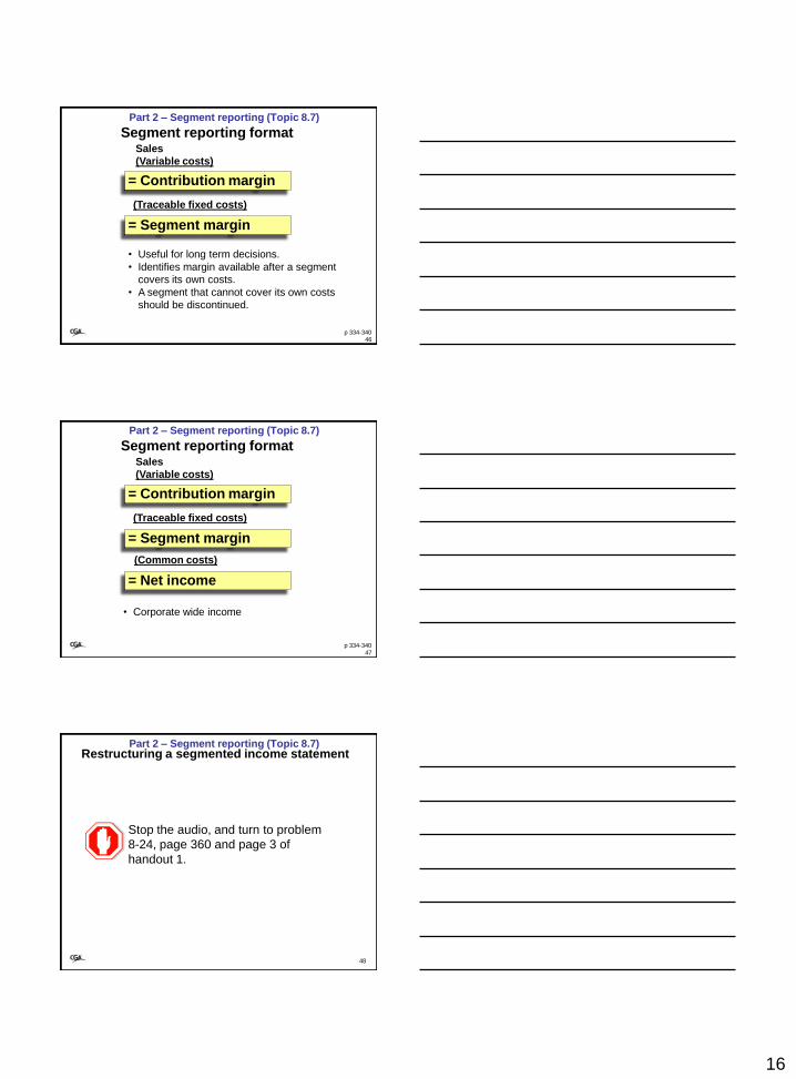
Part 2 – Segment reporting (Topic 8.7)
• Identifies what happens to profits as volume
changes.
• Useful for short run decisions such as temporary
uses of capacity. (chapter 12)
= Contribution margin
Sales
(Variable costs)
Segment reporting format
45p 334-340
16
Part 2 – Segment reporting (Topic 8.7)
• Useful for long term decisions.
• Identifies margin available after a segment
covers its own costs.
• A segment that cannot cover its own costs
should be discontinued.
= Contribution margin
Sales
(Variable costs)
(Traceable fixed costs)
= Segment margin
Segment reporting format
46p 334-340
Part 2 – Segment reporting (Topic 8.7)
= Contribution margin
Sales
(Variable costs)
(Traceable fixed costs)
= Segment margin
• Corporate wide income
Segment reporting format
= Net income
(Common costs)
47p 334-340
Part 2 – Segment reporting (Topic 8.7)
48
Restructuring a segmented income statement
Stop the audio, and turn to problem
8-24, page 360 and page 3 of
handout 1.
17
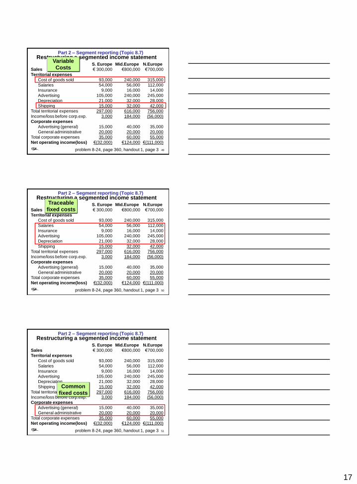
Part 2 – Segment reporting (Topic 8.7)
49
Restructuring a segmented income statement
S. Europe Mid.Europe N.Europe
Sales € 300,000 €800,000 €700,000
Territorial expenses
Cost of goods sold 93,000 240,000 315,000
Salaries 54,000 56,000 112,000
Insurance 9,000 16,000 14,000
Advertising 105,000 240,000 245,000
Depreciation 21,000 32,000 28,000
Shipping 15,000 32,000 42,000
Total territorial expenses 297,000 616,000 756,000
Income/loss before corp.exp. 3,000 184,000 (56,000)
Corporate expenses
Advertising (general) 15,000 40,000 35,000
General administrative 20,000 20,000 20,000
Total corporate expenses 35,000 60,000 55,000
Net operating income(loss) €(32,000) €124,000 €(111,000)
Variable
Costs
problem 8-24, page 360, handout 1, page 3
Part 2 – Segment reporting (Topic 8.7)
50
Restructuring a segmented income statement
S. Europe Mid.Europe N.Europe
Sales € 300,000 €800,000 €700,000
Territorial expenses
Cost of goods sold 93,000 240,000 315,000
Salaries 54,000 56,000 112,000
Insurance 9,000 16,000 14,000
Advertising 105,000 240,000 245,000
Depreciation 21,000 32,000 28,000
Shipping 15,000 32,000 42,000
Total territorial expenses 297,000 616,000 756,000
Income/loss before corp.exp. 3,000 184,000 (56,000)
Corporate expenses
Advertising (general) 15,000 40,000 35,000
General administrative 20,000 20,000 20,000
Total corporate expenses 35,000 60,000 55,000
Net operating income(loss) €(32,000) €124,000 €(111,000)
Traceable
fixed costs
problem 8-24, page 360, handout 1, page 3
Part 2 – Segment reporting (Topic 8.7)
51
Restructuring a segmented income statement
S. Europe Mid.Europe N.Europe
Sales € 300,000 €800,000 €700,000
Territorial expenses
Cost of goods sold 93,000 240,000 315,000
Salaries 54,000 56,000 112,000
Insurance 9,000 16,000 14,000
Advertising 105,000 240,000 245,000
Depreciation 21,000 32,000 28,000
Shipping 15,000 32,000 42,000
Total territorial expenses 297,000 616,000 756,000
Income/loss before corp.exp. 3,000 184,000 (56,000)
Corporate expenses
Advertising (general) 15,000 40,000 35,000
General administrative 20,000 20,000 20,000
Total corporate expenses 35,000 60,000 55,000
Net operating income(loss) €(32,000) €124,000 €(111,000)
Common
fixed costs
problem 8-24, page 360, handout 1, page 3
18
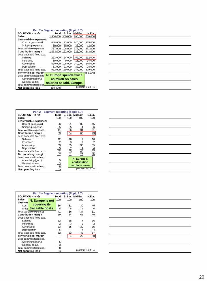
52
SOLUTION - In €s Total S. Eur. Mid.Eur. N.Eur.
Sales 1,800,000 300,000 800,000 700,000
Less variable expenses:
Cost of goods sold 648,000 93,000 240,000 315,000
Shipping expense 89,000 15,000 32,000 42,000
Total variable expenses 737,000 108,000 272,000 357,000
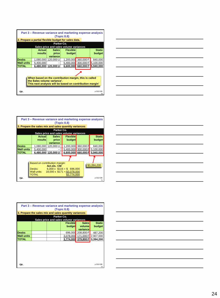
TOTAL 3,774,000 68,490U 3,842,490 448,290F 3,394,200
* rounded
78
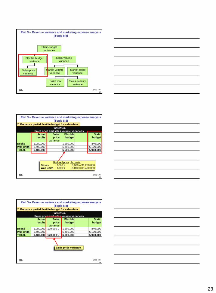
Part 3 – Revenue variance and marketing expense analysis
(Topic 8.8)
p 532-538
27
Static-budget
variances
Flexible budget
variance
Sales-volume
variance
Sales price
variance
Market volume
variance
Market share
variance
Sales mix
variance
Sales quantity
variance
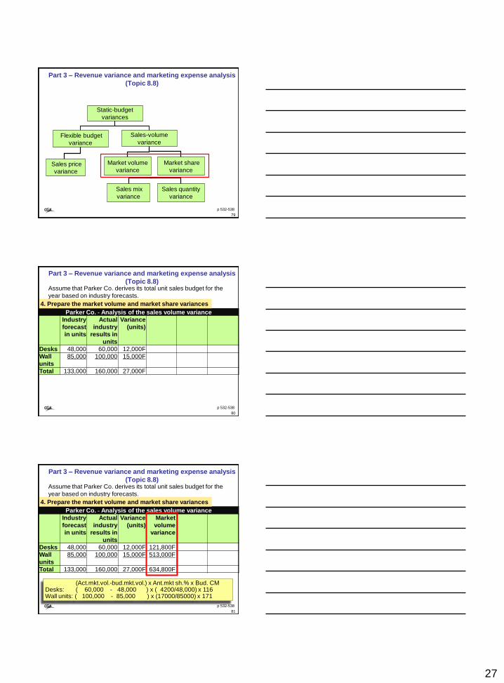
79
Part 3 – Revenue variance and marketing expense analysis
(Topic 8.8)
p 532-538
Assume that Parker Co. derives its total unit sales budget for the
year based on industry forecasts.
Parker Co. - Analysis of the sales volume variance
Industry
forecast
in units
Actual
industry
results in
units
Variance
(units)
Desks 48,000 60,000 12,000F
Wall
units
85,000 100,000 15,000F
Total 133,000 160,000 27,000F
4. Prepare the market volume and market share variances
80
Part 3 – Revenue variance and marketing expense analysis
(Topic 8.8)
p 532-538
Assume that Parker Co. derives its total unit sales budget for the
year based on industry forecasts.
Parker Co. - Analysis of the sales volume variance
Industry
forecast
in units
Actual
industry
results in
units
Variance
(units)
Market
volume
variance
Desks 48,000 60,000 12,000F 121,800F
Wall
units
85,000 100,000 15,000F 513,000F
Total 133,000 160,000 27,000F 634,800F
4. Prepare the market volume and market share variances
(Act.mkt.vol.-bud.mkt.vol.) x Ant.mkt sh.% x Bud. CMDesks: ( 60,000 - 48,000 ) x ( 4200/48,000) x 116Wall units: ( 100,000 - 85,000 ) x (17000/85000) x 171
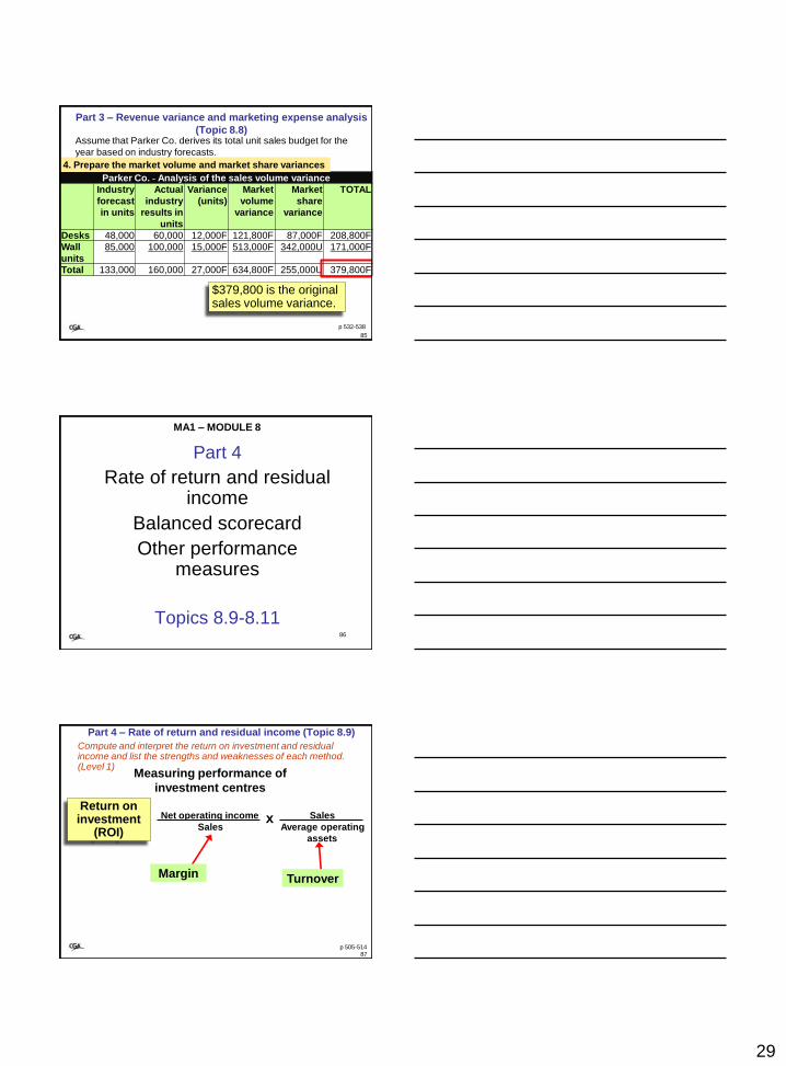
81
Part 3 – Revenue variance and marketing expense analysis
(Topic 8.8)
p 532-538
28
p 532-538
Assume that Parker Co. derives its total unit sales budget for the
year based on industry forecasts.
Parker Co. - Analysis of the sales volume variance
Industry
forecast
in units
Actual
industry
results in
units
Variance
(units)
Market
volume
variance
Desks 48,000 60,000 12,000F 121,800F
Wall
units
85,000 100,000 15,000F 513,000F
Total 133,000 160,000 27,000F 634,800F
4. Prepare the market volume and market share variances
82
• The total market size for desks has increased by 60,000-48,000=12,000 units
• Parker’s share of this is 8.75% (4200/48,000). That’s 1050 units• 1050 units x CM of $116 is $121,800 which means that Parker’s
share of the increase in the market size is $121,800.
Part 3 – Revenue variance and marketing expense analysis
(Topic 8.8)
Assume that Parker Co. derives its total unit sales budget for the
year based on industry forecasts.
Parker Co. - Analysis of the sales volume variance
Total 133,000 160,000 27,000F 634,800F 255,000U 379,800F
4. Prepare the market volume and market share variances
84
•Parker’s original forecast of 4200 units was 8.75% of the market. •At a market level of 60,000 units they should have sold (60,000x8.75%) 5,250 units to maintain their market share. •Instead they sold 6000 units. The increase of 750 units x $116 CM is $87,000 which is their increase in the share of the market for desks.
Part 3 – Revenue variance and marketing expense analysis
(Topic 8.8)
29
Assume that Parker Co. derives its total unit sales budget for the
year based on industry forecasts.
Parker Co. - Analysis of the sales volume variance