VLDBJournal,3, 401-444 (1994), Ralf Hartmut Giiting, Editor QVLDB 401 Management of Multidimensional Discrete Data Peter Baumann Received July 6, 1993; revised version received April 5, 1994; accepted May 20, 1994. Abstract. Spatial database management involves two main categories of data: vec- tor and raster data. The former has received a lot of in-depth investigation; the latter still lacks a sound framework. Current DBMSs either regard raster data as pure byte sequences where the DBMS has no knowledge about the underlying semantics, or they do not complement array structures with storage mechanisms suitable for huge arrays, or they are designed as specialized systems with sophis- ticated imaging functionality, but no general database capabilities (e.g., a query language). Many types of array data will require database support in the future, notably 2-D images, audio data and general signal-time series (I-D), animations (3-D), static or time-variant voxel fields (3-D and 4-D), and the ISO/IEC PIKS (Programmer's Imaging Kernel System) BasicImage type (5-D). In this article, we propose a comprehensive support of multidimensional discrete data (MDD) in databases, including operations on arrays of arbitrary size over arbitrary data types. A set of requirements is developed, a small set of language constructs is proposed (based on a formal algebraic semantics), and a novel MDD architecture is outlined to provide the basis for efficient MDD query evaluation. KeyWords. Multimedia database systems, image database systems, tiling, spatial index. 1. Introduction In the discipline of visualization, where the areas of computer graphics, image processing, computer vision, computer-aided design, signal processing, and user interface studies converge into one unifying framework for the processing of visual information (McCormick et al., 1987), several representations of a scene (an image in its most general meaning) are distinguished. Kr6mker (1991) proposes a visualization reference model that is particularly suitable for database investigations because classification is done along the data structures on hand (Figure 1). Three of the six layers introduced in this reference model are relevant for DBMSs that deal with Peter Baumann, Ph.D., is Assistant Head, Bavarian Research Center for KnowledgeBased Systems(FOR- WlSS), Orleansstr. 34, D-81667 Mfinchen, Germany.
Received July 6, 1993; revised version received April 5, 1994; accepted May 20, 1994.
Abstract. Spatial database management involves two main categories of data: vec- tor and raster data. The former has received a lot of in-depth investigation; the latter still lacks a sound framework. Current DBMSs either regard raster data as pure byte sequences where the DBMS has no knowledge about the underlying semantics, or they do not complement array structures with storage mechanisms suitable for huge arrays, or they are designed as specialized systems with sophis- ticated imaging functionality, but no general database capabilities (e.g., a query language). Many types of array data will require database support in the future, notably 2-D images, audio data and general signal-time series (I-D), animations (3-D), static or time-variant voxel fields (3-D and 4-D), and the ISO/IEC PIKS (Programmer's Imaging Kernel System) BasicImage type (5-D). In this article, we propose a comprehensive support of multidimensional discrete data (MDD) in databases, including operations on arrays of arbitrary size over arbitrary data types. A set of requirements is developed, a small set of language constructs is proposed (based on a formal algebraic semantics), and a novel MDD architecture is outlined to provide the basis for efficient MDD query evaluation.
In the discipline of visualization, where the areas of computer graphics, image processing, computer vision, computer-aided design, signal processing, and user interface studies converge into one unifying framework for the processing of visual information (McCormick et al., 1987), several representations of a scene (an image in its most general meaning) are distinguished. Kr6mker (1991) proposes a visualization reference model that is particularly suitable for database investigations because classification is done along the data structures on hand (Figure 1). Three of the six layers introduced in this reference model are relevant for DBMSs that deal with
Peter Baumann, Ph.D., is Assistant Head, Bavarian Research Center for Knowledge Based Systems (FOR- WlSS), Orleansstr. 34, D-81667 Mfinchen, Germany.
• The Symbolic Representation Layer deals with abstract scene descriptions, but without an explicit description of geometry and properties of the entities modeled. Example: A 3-D scene consisting of a house with a tree next to it might be described through the entities House and Tree with a relation- ship i s - n o r t h - o f between them. House could have attributes like #Floors indicating the number of levels, or address for its address.
• The Geometry~Feature Layer covers geometric descriptions, appearance prop- erties, and viewing parameters. Vector graphics would be a subset of such data structures. Example: On this level, the house/tree scene is described without the specific semantics of a "house" and a "tree," but with information about sizes, locations, or appearance. Thus, House in this view consists of (i.e., is bounded by) 2-D regions positioned in Euclidean space, its walls and roof having assigned individual surface properties like color and roughness. A complete scene description additionally requires one or more light sources with attributes color, intensity, and location.
• On the Digital Pixel Layer, a scene is discretized in both space and color, yielding a raster image. A raster image consists of a finite set of points in the discrete coordinate space Z a where each point has some value, its color, associated. Example: Adopting a specific point of view and viewing angle of the observer/camera, as well as a certain pixel resolution and color space, the geometric scene can be rendered yielding a raster image of house and tree.
From the point of view of conceptual modeling in databases, the Symbolic Layer is covered by semantic nets; the Geometry/Feature Layer is supported by vector databases, and entities belonging to the Digital Pixel Layer are maintained in image databases.
Let us elaborate on the difference between vector and raster representation of spatial data. It is important to realize that these representations are not only very different in terms of structures and operations; they indeed comprise substantially different kinds of information about the same real-world entity. This becomes evident when we look at the means for transformation between both representations.
Rendering a (2-D or 3-D) geometric model generates a raster image that depends on various parameters usually not captured in the geometry/feature information (e.g., the curve technique, Mortenson, 1985; and the illumination model, Bouknight, 1971; Gouraud, 1971; Phong, 1975) implemented in the renderer. Discretization of geometric elements implies a loss of geometric accuracy and structure information (e.g., does a long, dark shape in a raster image represent a line or a thin region?).
Feature extraction methods are designed to interpret raster images to recog- nize points, lines, and regions that are assumed to be encoded in the pixels. This works acceptably well in small universes of discourse (e.g., for technical drawings with their highly stylized graphical vocabulary). However, there is no algorithm that
VLDB Journal 3 (4) Baumann: Management of Multidimensional Discrete Data 403
Figure 1. Kr6mker's structure model for visualization
I I~ I i~
monitor ~ camera
user
application representation
symbolic representation
geometry/feature representation
digital pixel representation
analog electrical representation
analog optical representation
I ........ ,~:~!~ processing unit
storage unit
data flow
performs reasonably well on any kind of image and under all circumstances; above all, images frequently contain information that cannot be cast into points, lines, and regions bounded by lines, because the boundary cannot be recognized without doubt (e.g., tumors in medical imagery), or because there is no clear boundary (e.g., density distributions such as clouds in weather satellite images; Figure 2).
404
Figure 2. Landsat infrared image of Coburg/Germany
In summary, both vector and raster representation are important for spatial data management, because each of them has specific strengths and weaknesses; moreover, both representations are independent from each other in the sense that there is no lossless transformation between them.
DBMS support for raster data is indispensable, because such structures appear in virtually all fields of database application. Office applications, CAD drawing management, remote sensing, environmental planning and control, medical imag- ing/picture archiving and communication systems (PACS), historical and geographic information systems, and scientific visualization, to name but a few, require database support to an increasing degree. In fact, any phenomenon whose nature is analog finally appears as discrete data of a specific dimensionality when sampled by a sensor and fed into an information processing system. The main characteristic of such data is that they form regular d-dimensional arrays that are frequently too big to fit into main memory as a whole. We call such structures multidimensional discrete data (MDD).
The consequence is that a general-purpose DBMS must support both vector and raster data, and that the DBMS itself cannot accomplish the transformation among them. Of course, application-specific DBMSs may incorporate functionality for mixed vector/raster manipulation.
VLDB Journal 3 (4) Baumann: Management of Multidimensional Discrete Data 405
Other articles in this special issue deal with vector graphics. A lot of investigation has been carried out on database management of vectorized data, and there has been considerable progress made in presentation, modeling, and storage management. Here, we focus on MDD management, which has received comparatively little attention in the database community. The common approach is to store raster images (which comprise the pivotal MDD application area) as Blobs (binary large objects) or longfields (i.e., variable-length byte strings with no further structure imposed). Regarding highly organized structures like two-dimensional matrices of integers as unformatted and treating them as linear byte strings already unveils that a profound framework for such structures is still missing.
Due to this deficiency in structural knowledge, MDD cannot be involved in search criteria (e.g., "select all X-ray images where, in a region specified by a given bit mask, intensity exceeds a certain threshold value," and they cannot be processed in a fashion such as "retrieve only the upper right 200 by 200 part of a several-Megabyte satellite image," or "extract all pixels in the x/z plane of a volume tomogram at a certain position y0.")
Moreover, most systems lack data independence, and can deliver images only in exactly the same byte stream in which they have been written. At first glance, employing an image interchange format like TIFF, GIF, or JPEG seems to be the solution; however, this usually requires spooling the result array received from the server into an intermediate file to decode it--a considerable overhead which should be avoided. Image display routines supplied by window management systems expect unencoded, uncompressed arrays of pixel values. Instead of relying on one of the many existing data exchange formats, data should be delivered in a format directly processable by the application program. Especially in heterogeneous networks coming up with open multimedia environments, data independence is an important prerequisite.
Besides the lack in functionality, an immediate consequence of mapping d- dimensional data to linear byte streams is inefficient storage access when only part of the data are addressed. Consider a 2-D image stored in a long field. The image is linearized by storing it line by line on disk. Access to the shaded part of the image in Figure 3a requires access to different places on disk, which can be widely scattered, depending on the selectivity of the query (Figure 3b).
To remedy this, an image database system must offer comprehensive MDD support. On the conceptual level, this means structure definition of arrays over arbitrary pixel types, not just a predefined selection of pixel types such as integer and real . A coherent, orthogonal set of operations must be available on such array types, and must be powerful enough to express image retrieval and manipulation in a descriptive, optimizable manner. The physical database layer must support the array concept by providing efficient access methods and a collection of compression mechanisms for d-dimensional arrays of basically arbitrary size. Concealment of these internal storage structures (i.e., data independence) is an essential prereq- uisite for cooperative, open multimedia environments distributed over heterogeneous
° ° ° • ° ° ° o ° o ° ° ° o ° • ° ° ° ° ° ° ° ° ° ° o ° ° ° ° ° ° . . . . . . o ° ° ° . . . . . . ° o
. . . . I . . . . . . . . . . . . . . . . . . . . . . . . . . . . . . . . . . . . . . . . . . . I . . . . . . . . . . . ° ° ° ° o ° o ° ° ° o o ° o • o . . . . . . ° ° ° o ° o ° o o ° 1 o ° ° ° o • ° ° o ° • • ° ° • ° ° o o o o o o o ° o o
° ° ° ° • ° ° ° ° ° ° ° ° ° • ° 1
networks, because only then can image structures be transmitted and reassembled appropriately according to the target machine's representation needs.
The purpose of this article is to state the requirements of MDD management and to propose an approach to enhance DBMSs with MDD capabilities. Because this work originated from projects around the research DBMS APRIL (Baumann and Kfhler, 1989), we discuss MDD definition and manipulation in the context of APRIL. However, any conceptual model could be augmented this way, be it relational, semantic, or object-oriented.
The remainder of this article is organized as follows. In Section 2, we state requirements of MDD modeling in databases. In Se, ction 3, we review related work.
VLDB Journal 3 (4) Baumann: Management of Multidimensional Discrete Data 407
Table 1. Images of different dimensionality
dimensions application area examples
scalar time series audio data, environmental data,
temperature curves, EEG
2-D images fax, satellite images, medical imagery
2-D animation flight simulation, cartoons,
commercials, education
3-D data sets hydrological, meteorological, and
astrophysical simulation results
volumetric time series time-variant versions of 3-D examples
ISO/IEC PIKS
(Programmer's Imaging Kernel System) type BasicImage
Next, we develop an algebraic formalism for MDD description and manipulation (Section 4), which serves as the basis for a set of language concepts proposed in Section 5. An architecture suitable for this conceptual model is presented in Section 6. We summarize our findings in Section 7.
2. Requirements
In this section, we develop the structural and operational requirements of conceptual MDD modeling in databases. Although investigation concentrates on 2-D image structures and operations, the results apply to MDD of any dimension.
2.1 Image Structures
Images form d-dimensional arrays over some base type (which is referred to as pixel type for 2-D and voxel type for 3-D); Table 1 lists examples of the most common dimensionalities. Currently, the highest number of dimensions occurs in the ISO/IEC imaging standard Programmer's Imaging Kernel System (PIKS; International Organization for Standardization, 1993) where the generic image structure BasicImage consists of three geometric dimensions x~ y, and z, a time dimension, and a channel dimension (an RGB image, for example, occupies three channels); all other image types are obtained from such a 5-D image through projection.
Non-rectangular images like sonograms (Figure 4) are, in practice, embedded into a minimal enclosing rectangle, hence there is no undue limitation when the rectangularity imposed by arrays is maintained.
Table 2 gives an overview of common 2-D image geometries and color schemes arising in various application areas. Binary, gray-scale, and red-green-blue (RGB)
408
Figure 4. Sonogram of a fetus
pixel types are well-known color representations. For satellite images, the visual band covered by RGB is extended with an infrared and several UV channels. Similar constellations occur in the prepress area where images are electronically processed before being printed. A subtractive color scheme is used, which is based on cyan, magenta, and yellow. In practice, a sufficiently dark black cannot be achieved by superimposing these colors, so a separate black channel is added. However, for superior print quality, schemes with up to twelve colors are not uncommon.
However, pixel information does not necessarily denote a color value; an arbitrary semantics (e.g., a reference to an entity somewhere else in the database) can be associated with a pixel. PICDMS (Chock et al., 1984) exploits this to mark regions making up a country in image-based geographic maps. Sonar and radar images encode the target object distance in the intensity value. Matrix-valued pixels are frequently used in the prepress area to describe color values through binary subpixels, and in graphics systems to reduce aliasing.
VLDB Journal 3 (4) Baumann: Management of Multidimensional Discrete Data 409
Table 2. Image types in different application areas
G3 fax (DIN A4)
HDTV still image
(Eureka format)
VGA
scanned slide
Medicine:
tomogram
X-ray image
Satellite images:
Landsat MSS
Landsat TM
MOMS
SPOT
and
prepress
geometric color pixel data volume
resolution resolution data type (uncompressed)
1728x1083
1920x1152
640x400
- 1024x768
3000x2000
2562-5122
<20482
3240x2340
7020x5760
6912 per line 60002
30002
2000x3000 - 150002
and more
1 bit
4+2+2 bit
e.g., 16 bit
24 bit
12 bit
12-16 bit
4x8 bit
7x8 bit
2x8 bit
lx8 bit
3x8 bit
4xl-4x8
and more
binary
YChCr
RGB,
color table
RGB
gray-scale
gray-scale
multispectral
multispectral
multispectral
panchromatic
RGB
CMYK
and others
500 kB
210 MB
e.g., 480 kB
18 MB
98 kB-392 kB
<8,4 MB
30 MB
283 MB
variable
36 MB
27 MB
24-900 MB
and more
The underlying pixel type remains constant over the image lifetime. Image size, however, shows much individual variation, and sometimes may change during image lifetime. Characteristic are the huge array sizes, which vary between 640x400 (VGA images) and 7020x5760 (Landsat TM images).
2.2 Image Operations
Existing imaging formalisms like AFATL Image Algebra (Ritter et al., 1990), an algebraic framework for the formulation of image and signal processing algorithms, provide useful insights concerning the operators on MDD. In image algebra, an image (MDD object 1 in our terminology) is a function
a: X---+ C
from a coordinate set XCT~ a into some algebraic system C called color space. An
1. We use the notion of an object here in a naive way to circumvent all discussion about object-oriented issues.
410
element (x,b(x)) is called apixel. Operations on and between images are the natural induced operations of C. On real-valued pixels, for example, these are the unary and binary operations such as addition, multiplication, and maximum. Thus, the addition of two images a and b for C = T~ is giwm by elementwise addition:
a + b = { (a~c (x)) I c(x) = a (x) + b (x),x E_--X}
In general, any unary function f: B ~ C induces a function f: B X ~ C X defined a s
f ( a ) = ( (x,b (x)) I b (x) = f ( a (x)),x E X }
and any binary function g: B, C ---r D induces a function g: B X, C X ~ D x given by
g (a,b) = { (x,c (x)) I c (x) = g (a (x),b (x)),x C X }
In the same way, pixel-level predicates can be lifted to predicates on images; note that the resulting pixel type substantially differs from the input pixel type. A simple example is thresholding, where the resulting image has a pixel value of 1 iff the original pixel value is greater than some threshold value t, and 0 otherwise. This is denoted as
X>t (a) = { (x~b (x)) I b (x) = i fa (x) > t then 1 e lse0f i , x C X }
Viewing images as functions gives rise to operations that express some important mathematical notions, namely domain, range, restriction, and extension. The set of coordinates on which an image a: X ~ C is defined (i.e., its domain) is denoted by
Domain(a) = X
The set of values actually assumed by the pixels of image a, (i.e., the range of a), is
Range(a) C C
The restriction of image a to a subset Y of X, which produces a cutout of a, is denoted by
alY = { (x,b (x)) I b (x) = a (x),x E Y }
Note that Y is not constrained to be specified through coordinate boundaries like Y = { (Xl, x2) E X ] 5 < Xl < 20 }; it might just as well depend on some image property such as Ya = { x E X I a(x) C C' }.
Let X be the coordinate set of image a, and Y be the coordinate set of image b where X is a subset of Y. Then, the extension of a to b on Y is that image which corresponds to b except that all pixels of the X area are replaced by a pixels. Formally, it is defined by
a[ (b'Y) = { (x,c(x)) [ c(x) = a(x) i fx E X, c(x) = b(x) i fx C Y \ X }
VLDB Journal 3 (4) Baumann: Management of Multidimensional Discrete Data 411
The most powerful tool of the image algebra from the point of view of image processing applications are templates and template operations. Informally speaking, a template operation allows images to be derived in a way that the resulting pixel values depend not only on the original pixel value, but also on a certain neighborhood of the original pixel; the template determines the pixel neighborhood and, at the same time, applies weights to the values. The resulting image may be of an entirely different shape, size, and dimension.
Instead of presenting the formalism, which would occupy too much space, let us look at a simple, yet typical, example for such an operation. The Sobel edge detector, a kind of high pass filter, uses two templates tx and ty, which can be depicted as 3x3 matrices with coordinate sets {-1,0,+1}2:
-1 0 +1 +1 +2 +1
= -2 0 +2 ff = 0 0 0
- 1 0 +1 -1 -2 -1
Let the color space C of a be T~, assume X as a's coordinate space, and let t be a template with coordinate set Y. For templates of the kind shown above, the right product of a with t is defined as
a * t = ( (x,b (x)) I b (y) = ~ a (x+y) * t (y),x E X } y6Y
where the second * denotes multiplication in T~. Using this definition, and with the aid of the induced function 1.1 for the magnitude, the Sobel filter is expressed (within a scaling factor) as
Sobel(a) = l a* txl + l a* tyl Figure 5 shows a gray-scale image and its Sobeled counterpart.
2.3 Image Modeling from a Database Point of View
Section 2.1 showed that the data structure underlying an image always can be viewed as a homogeneous, rectangular d-dimensional array over some arbitrary pixel data type. While it is feasible to fix the array base type at type definition time, the large number of different image sizes suggests open array boundaries, which can vary dynamically. This allows several database operations, which are usually provided on image instances, to become schema-level operations. For example, querying the color space of an image means accessing the image array's base type. The remaining instance-level operations can be classified into the following basic categories, using database terminology:
• Retrieve the current size of an image (image range).
• Extract a part of an image (image restriction). Because we restrict ourselves to rectangular images, only rectangular part extraction is required.
412
Figure 5. Detecting car silhouette using Sobel edge detector
• Retrieve some image a where for each pixel coordinate x in the original image some derived value f(a(x)) is substituted (unary induced operations).
• Retrieve an image f(a,b) which is the result of the combination of two input images a and b (binary induced operations, image extension).
• Retrieve some image a as before, but additionally consider some neighborhood env(a,x) of each pixel x in the computation of the resulting pixels (template operations).
Image access can be refined according to the pixel traversal sequence required by the application (i.e., the order in which the result is built). The traversal sequence is:
• relevant and/or known in advance (e.g., line by line access in ray tracing algorithms).
• not predictable (e.g., stochastic texture generation algorithms or contour finders in image recognition systems).
It is very important that traversal sequence is not dictated by the query, because only then does an optimizer have the chance of finding an optimal access sequence with minimal disk traffic. Obviously, the first access scheme offers the best potential for optimization, and the second scheme may allow some influence, whereas the third scheme is unlikely to benefit from optimizations.
How relevant are these categories for database management systems? Obtaining range information is indispensable for obvious reasons. Image restriction is an important means to condense huge data sets. Image extension is necessary to allow the growth of variable-sized images in updates. Unary and binary induced functions can be provided as a consequence of the enriched semantics--the additional structural knowledge allows more operations. These capabilities heavily depend on
VLDB Journal 3 (4) Baumann: Management of Multidimensional Discrete Data 413
the power of the overall data model: in the classical relational model, only a fixed, quite small set of operations can be induced. Extensible systems, on the other end of the spectrum, allow both system-defined and user-defined pixel operations to be induced.
Besides conceptual considerations concerning the semantic richness of the op- erational model, there is an effect of changed access characteristics on the networks load. With this respect, image restriction represents the perhaps most important function, because it reduces client memory space and computation overhead and especially networks traffic. Without this functionality, the whole image has to be sent to the client site for evaluation. For updates involving image extension, induced operations, and template operations, transfer savings arise from the fact that image processing occurs near the information source and sink; otherwise, expensive image transfer from server to client and back again must be performed. Another advantage is that the client site does not have to intermediately store the complete original image(s) to be retrieved or updated. Thus, main memory is allocated only for the information actually requested, which frequently occupies only a fraction of the overall image size.
Range querying, image restriction, image extension, and induced operations comprise a set of easy-to-grasp operations even for users not familiar with image processing. Generalized template operations, on the other hand, require considerable knowledge in the imaging area and also impose overhead on the conceptual model-- although several operations with immediate practical relevance can be expressed using templates, such as:
• smooth or enhance contours in an image; • extract only the even or only the odd lines of an image for interlaced display; • flip a slide which has been scanned wrong side up.
It might, therefore, be feasible to not provide the full power of template opera- tions, and to offer specialized operations suitable for the most common application cases which then can be implemented in a more efficient manner. Alternatively, an extensible database system could allow an experienced database programmer to use template operations for providing easy-to-use application-specific functionality.
In summary, we claim that range, restriction, extension, and induced functions are mandatory for image management. Template operations are optional; further investigation is necessary to determine to what extent and in what form they are best provided.
3. Related Work
In this section, we describe relevant work in the field. Since 2-D images represent the pivotal application of MDD, it is the area of image databases that we must consider. Again, we first investigate image structuring methods and then the operations offered on such structures.
414
3.1 Image Structures
In the first approach to introduce images to databases, an operating system file encoded the actual image in some specialized file format, consisting of a descriptional header followed by the "raw" image data themselves (e.g., Grosky, 1984). Gradually, this has shifted from using proprietary image formats to using one of several common image exchange formats. In any case, however, in the database itself only a reference to the file is kept. This kind of established workaround is still by far the most common technique in office information systems (Appelrath and Eirund, 1990), clinical picture archiving and communication systems (PACS) (Osteaux, 1992; Foord and Tomlinson, 1993), and multimedia systems (Stucki and Menzi, 1989). Though fast and simple, there are several shortcomings to employing files external to the DBMS: These data cannot use traditional database services for transaction control and recovery; there is no data independence at all; such data cannot be part of search conditions; and there can be no computed query result.
A better integration of MDD into the normal database traffic is accomplished through long fields (Lorie, 1982). Attributes of type long field allow for byte strings of variable extent with size limits up to 2 GB. Storage management is under full DBMS control, thereby allowing transaction and recovery services on long attributes.
However, raster images essentially are not byte sequences, but (2-D) matrices. Some authors therefore propose matrices over some base type as a new attribute domain. Lien and Harris (1980) used integer numbers ranging from 0 to 255 for the array base type; this is obviously insufficient for many practical cases. PICDMS (Chock et al., 1984) offers in t ege r , : f loat , b i t [ n ] , and byte[n] . Although conceptually richer, this model cannot express the composed pixels that occur in color images (e.g., with the RGB color model) and satellite images (Landsat TM pixels consist of seven sensor values), except as an unstructured byte string; extraction of pixel components, for instance, is left to the application. Meyer-Wegener et al. (1989) tried to overcome this by adding encoding information to pixel types of the kind b i t [n] (e.g., RGB_REAL_32 and IHS_INT_8 for different color models and color depth ranges). However, such a system is limited to a predefined enumeration of pixel types.
Most models are restricted to matrices (i.e., 2-D arrays). A specialty of PICDMS is its so-called image stacks, consisting of an arbitrary number of equally-sized 2-D raster images addressed by name (so this structure essentially is more like a record than a stack). For each layer, the pixel type can be set up individually. Several semantic and object-oriented models which support array data types (e.g., Kemper and Wallrath, 1987) constrain them to very small sizes, such as 4x4 matrices; sizes of several millions of elements cannot be handled efficiently. Array structures of arbitrary dimensionality with both fixed and variable bounds are supported by the EXTRA/EXCESS system described by Vandenberg and DeWitt (1991); however no evidence is given that internal storage support is provided for huge arrays.
VLDB Journal 3 (4) Baumann: Management of Multidimensional Discrete Data 415
Several specialized image management systems support huge arrays on the internal level, however, without a query language interface. Omolayole and Klinger (1980) suggested using a recursive, quadtree-like image decomposition into axis- parallel boxes. Decomposition is done feature-based using Kirsch edge detectors, thresholding, and other feature extraction mechanisms. A library of image processing functions providing transparent image tiling is described by Tamura (1980). Data access is independent from physical organization and the partitioning policy adopted during insertion.
3.2 Image Operations
Byte sequences as attribute domains offer only sequential access, sometimes with a cursor concept for piecewise manipulation (Lorie, 1982). Systems tailored for multimedia applications frequently provide specific raster image support through a fixed set of image operators (Chang and Fu, 1980; Stucki and Menzi, 1989). Besides storing and loading the whole image, they provide a library of image processing functions such as scaling, rotating, contour finding, or thresholding. The IQ system (Lien and Harris, 1980) also offers functional composition of such basic operators, but not in the sense of a full query language. In particular, queries over such data are not optimized.
PICDMS comes with a query language on image stacks (Joseph and Cardenas, 1988). For image manipulation, a command language is supplied, which accomplishes traversal of the pixel coordinate set and stack layer access by moving a window across the pixel plane stack (Figure 6). The following sample query takes a Landsat multispectral image and computes the difference between bands 4 and 5 (due to the simple algorithm, the scan window in this case contains only one pixel):
ADD (IMAGE DIFF FIXED (8,0)),
DIFF = BAND4 - BAND5,
FOR (BAND4 NOT = BLANK) AND (BAND5 NOT = BLANK);
In the course of the query evaluation, an 8-bit integer image named DIFF is inserted into the database, which contains tffe difference of the pixel values of both bands for each position where both pixel values are defined. The limits of this language are reached when it comes to the composition of operations. Operations other than projections are comparatively complicated. Nevertheless, a remarkable advantage is the specification of pixel inspection without any sequence prescription.
EXTRA/EXCESS offers a full query and manipulation language on an algebraic basis (Vandenberg and DeWitt, 1991). Besides the extraction of subarrays from arbitrary dimensional arrays, several operators are suggested which correspond to those on sets, bags, and lists. Most remarkable, induced operators are expressible through an operator which applies pixel operations simultaneously to all array elements.
416
Figure 6. PICDMS image stack access through the scan window
[ Z
I I
scan window
3.3 Summary
Work on image databases is being performed in the; imaging and database domains. Proposals from the former area offer extensive lists of operations on image data types, but are usually tailored to special application areas and, hence, rely on some fixed schema, mostly without an explicit data model. Conversely, in the database area an integration of images into well-established techniques is tried, but the support reached is far from the operational flexibility offered for the classical attribute domains. Due to the semantic restriction to byte strings, neither external (e.g., data independence) nor internal (e.g., index structures) support is possible. Those proposals that indeed offer MDD capabilities do not provide storage mechanisms adapted to the huge array sizes on hand.
4. Formal Semantics for MDD Definition and Manipulation
The formal framework for MDD definition and manipulation relies on set algebra. It is similar, but not identical to the image algebra framework: a subset has been chosen in accordance with the requirements listed above, and the model has been adapted to the specific needs of database management.
We consider arrays or expressions yielding arrays a with dimensionality Dim(a)=d over base type Base(a)=B and a coordinate space Range(a) = { r=(rl,...,rd) 1 mini <ri maxi, l < i < d } C Z d. A coordinate vector x=(xl,...,Xd) C Range(a) specifies an array element location, the i-th range component addressed as Rangei(a).
VLDB Journal 3 (4) Baumann: Management of Multidimensional Discrete Data 417
The null value of type B will be denoted as nullB. For some vector v holding at least i items, vi represents the i-th element of v.
Array elements, in the sequel called cells, are uniform (i.e., of the same base type B). Moreover, all hyperplanes contain the same number of elements, so that an array always forms a hyper-rectangle with axis-parallel boundaries in the d-dimensional coordinate space ( remember that we restricted M D D to a rectangular shape). An array is said to be of fixed size if its boundaries are prescribed for each dimension. It is said to be of variable size if its boundaries can vary in at least one of its dimensions. This notion will be formalized in Section 4.2.
We first introduce a pure value semantics to describe functional operations, then we add an update semantics to state the rules for updating a whole or part of an array.
4.1 Value Semantics
We use a purely functional semantics without any side effect. The value-based constructs provided are constants, trimming 2 to describe array cutouts, projection to reduce dimensionality of an array, induced operations, and predicate iterators to condense Boolean arrays to single Boolean values.
4.1.1 Constants. Let X C Z d be a finite coordinate set. The constant array over X with values k C B is defined as
ck ,x = { (x,k) I x c x } Base (Ck,X) = B Dim(ck,x) = d Range (ck,x) = X
Constant images mainly serve to prepare an array of a specific size whose cells subsequently can be modified. For example, a uniform background can be generated this way. The unit array Cl,X, in particular, is used for scaling purposes.
4.1.2 Trimming. The trim operation produces a cutout of an array with axis-parallel boundaries along the i-th dimension (Figure 7) without affecting the dimensionality. If t and u are integer numbers with t<u and {t..u} C_ Rartgei(a), then the semantics of array a t r immed to (t,u) in the i-th of d dimensions is given by
trimi,t,u(a ) = { (x,b(x)) I b(x) = a(x), x E Range(a), xi E {t..u} } Base(trimi,t,u(a)) = Base(a) D±m(trirai,t,u(a)) = Dim(a) = d
i -1 d Range(trimi,t,u(a)) = × Rangej(a) × {t..u} X X Rangek(a)
j = l k=iq-1
2. The trim operation has its roots in the programming language ALGOL 68 (van Wijngarden et al., 1969).
418
Figure 7. Focusing on Charlie Parker's head using trim operation
4 .1 .3 Projec t ion . Projection of a d-dimensional array generates a (d-1)-dimensional hyperplane. Concerning the result data set, projection corresponds to a single slice trim operation. On the metadata level, however, there is a difference between trim and projection, because the coordinate dimension is reduced by one, thus changing the array structure. Formally, the projection of a d-dimensional array a along the p-th dimension at xp =r is given by
projp,r(a) = { (y,b(y)) I b(y) = a(x), x = ( y f , ... ,Yp-1 , r, yp, ... ,Yd -1 ) ,
Y=(Yl,-.. ,Yp-1, Yp, ... ,Ya-1), x e Range(a) } Base(projp,r(a)) = Base(a) D i m ( p r o j p , r ( a ) ) = Dim(a) - - 1 = d - - 1
p - 1 d R a n g e ( p r o j p , r ( a ) ) = X R a n g e i O ) X X R a n g e k ( a ) C ~ j d - 1
i=1 k = p + l
4.1.4 Induced Operations. Every operation on the array base type induces a corresponding array operation that delivers the array where the base function has been applied to each cell.
VLDB Journal 3 (4) Baumann: Management of Multidimensional Discrete Data 419
Given a function f: B ---+ C, the induced operation f is defined as follows:
f (a) = { (x, b (x)) I b (x) = f (a (x)),x 6 Range(a) } Base (f (a)) = C Dim (f (a)) = Dim (a) Range (f (a)) = Range (a)
This definition can easily be extended to binary functions. Consider two arrays a and b with equal dimensions and sizes (i.e., Dim(a)=Dim(b) and l~ange(a)=Range(b)), and, not necessarily equal, base types Base(a)=B and Base(b)=C. Then, for some function g: B, C ---+ D, the induced operation g is given by:
g (a,b) = { (x, c (x)) [ c (x) = g (a (x), b (x)), x 6 Range (a) } Base (g (a, b)) = D Dim ~ (a, b)) = Dim (a) = Dim (b) Range (g (a,b)) = Range (a) = Range (b)
4.1.5 Predicate Itemtors. Especially for induced comparison operations, it is nee- essary to have a means for condensing the resulting Boolean array in queries such as: "is the image all black?" We provide conjunction and disjunction of cells; 3 more complicated cases can be derived. The o~ operator resembles the conjunction: It evaluates to true iff all cells contain true. The dual operator cr returns true iff there is at least one cell with a true value. Formally speaking, for an array a with Base(a)=Boolean, a and cr are defined as:
~(a) = Vx6 Range (a): a (x) if(a) = 3x6 Ftange (a): a (x)
4.2 Update Semantics
We now consider array-valued variables (which may appear as relational attributes as well as object variables) and state the conditions for updating such variables. The old and new value of variable a will be denoted as a.old and a.new, respectively. None of the operations changes the array base type B or the array dimension d.
To properly treat arrays with variable size, we formalize the notion of fixed and variable size arrays. Let Dim(a) = d for an array variable a. The variability indicator V(a) is then defined as follows:
V(a) = (1,'1, ... ,I'd) E { fiX, var }d
where for l < i < d
vi = fix if a has finite size limits in dimension i, vi = var if a is unbounded in dimension i.
3. N o t e tha t nega t ion is an induced opera t ion .
420
A variable a is said to be of fixed size if all vi are ]be; it is said to be of variable size if there is at least one vi with vl = var.
Function Range is interpreted as the boundaries of array variables as set forth in the structure definition. For fixed-size array types, the domain of Range is the d-dimensional cross product of compact integer sets as introduced earlier. For variable-sized array types, Range is unconstrained and, hence, set to Z a. We introduce the new function range to denote the current array limits which, in case of a variable-sized array, may differ from the value delivered by Range. For array values (constants or right-hand sides of assignment expressions), the result of range and Range always will be identical, because a pure value has a fixed size.
4.2.1 Initialization. Every array variable must be initialized before any other op- eration can be applied (in practice, this can be done at tuple insertion or object instantiation time, respectively). The main task is to set the actual range to the predefined array limits and preset all cells with null values (fixed size), or to set the actual range to an empty set (variable size).
Formally, initialization of a d-dimensional array variable a over base type B with range Range(a) is defined as follows:
Preconditions: none.
Postconditions: init(a) --~
a.new = { (x,a(x))la(x) = nullB, x E range(a) }
Base (a . new) = B
Dim (a.new) = d d
range (a.new) = ×Ri i=i
where Ri = l~angei(a.new) if Vi(a)=fix, Ri = {} if Vi(a)=var.
For a fixed size array, it follows that range(a .new)= Range(a). For a variable size array, the initial content is empty, because the extension in the variable dimensions is zero.
4.2.2 Assignment. In an assignment ass(a,v), a variable a of some array type receives an array value v. Besides matching base types and dimensions, ranges for all fixed dimensions must match; in variable dimensions, the range of the array value assigned will be adopted.
Preconditions: Base (a.old) = Base (v)
Dim (a. old) = Dim (v)
range/ (a.old) = Range/ (v) for all l<i<d where Vi(a.old) = fix
VLDB Journal 3 (4) Baumann: Management of Multidimensional Discrete Data 421
Figure 8. Extending a 2-D array through partial assignment
null v
a.old null a.new
Postconditions: a s s ( a , v ) ---+
a.new = { (x,a(x)) I a(x) = i fx 6 Range(v) then v(x) else a(x)fi, x e range(a.~ew) }
Base(a.old) = Base(v) Dim(a.new) = Dim(a. old) range(a.new) = range(a.old) for all l<i<d where Vi(a.old) = fix range(a.new) = Range(v) for all l < i < d where Vi(a.old) = var
4.2.3 PartiaIAssignment The operation pass(a,v,M) serves to replace part of ar- ray variable a ' s current contents by array value v where M is a set of coordinate pairs mapping v coordinates to a coordinates. For each cell (x;a(x)) with loca- tion x=(x l , ... ,XDim(a)) 6 range(a) , which is to receive value v(y) with position Y=(Yl, ... ,YDim(v)) 6 Range(v), the pair (x,y) appears in M. Note that vectors x and y may well have different dimensions.
As mentioned earlier, domains must match. In the case of a fixed array, the substitution area must lie completely within the array limits; a variable array, however, can be extended whereby new cells not covered by the replacement values will receive null values. Figure 8 depicts the 2-D case.
Let R stand for the range resulting from overlaying a with v directed by M:
d R = X { mini(MxU range(a.old) ).. . raax i (UxU range(a.old) ) }
i=1 where
422
M X = { x l (x,y) e M } mini(X) = rain( { xil x=(xl,...,Xd), x E X } ) for l< i<Dim(a .o ld) maxi(X) = max( { xil x=(xl,...,Xd), x 6 X } ) for l< i<Dim(a .o ld)
Then the partial assignment of array v to array a at position p is defined as follows:
Preconditions: Base(a.old) = Base(,) Dim(a.old) = Dim(v) Rangei(a.old) ~ { Xil (x,y) 6 M } if Vi(a)=f ix for some l< i<Dim(a .o ld )
Postconditions: pass(a,v,M) --~
a .new = { (x~a(x)) J a(x) = if (x,y) 6 M then vCv ) elsf x c range(a, old) then a. old(x)
else nu l lB f i , x E range(a.new), y C Range(v) }
Base(a.new) = Base(a. old) Dim(a.new) = Dim(a.old) range(a.new) = range(a, old) if a is of fixed size range(a .new) = R if a is of variable size
5. An MDD Query and Manipulation Sublanguage
We now introduce an MDD definition and manipulation language, which forms a database sublanguage suitable for the description and manipulation of images and other MDD types.
Because MDD research originated from extending the prototype ooDBMS APRIL (Baumann and K6hler, 1989), we use the type definition and query language of APRIL to tie the concepts to some concrete model and query language. Basically, however, any conceptual model, be it relational, semantic, or object-oriented, could be augmented this way.
The conceptual model of APRIL offers objects which are identified through an externally visible object key. Through an object type definition, the following object constituents can be specified:
• A set of attributes. All C base types and constructors, such as enumerations, records, and arrays with arbitrary nesting are available; pointers have been substituted by the safer and more expressive successors concept (see below).
• A longfield, the so-called object contents. In the APRIL version we started with, the contents is viewed as the usual byte string with no further semantics imposed, but with the ability to grow and shrink dynamically.
VLDB Journal 3 (4) Baumann: Management of Multidimensional Discrete Data 423
A successors clause (Baumann, 1989; Zhou and Baumann, 1992), describing the set of admissible object references (w.r.t. referenced object types, cardi- nality, and possible variants). APRIL checks admissibility of insertion and keeps track of the completeness status of an object, which can be queried at any time. In automotive design, for example, a complete object of type Car consists of one Chassis object, either a DieselEngine or an 0ttoEngine (but not both), and an even number of Wheels (at least four). The corresponding object type definition looks as follows:
typedef objec t { successors
Chassis and ( DieselEngine xor OttoEngine )
and 2..* ( 2 Wheel ); } Car;
Both object hierarchies (i.e., directed acyclic graphs) and general object graphs are modeled this way.
Multiple inheritance between object types is provided through a specialization operator. The generic operation set supplied with the model is augmented with type-specific attribute store and retrieve operations that accomplish transformation between the APRIL transfer format and the application program representation. Database access is performed through a library of C routines or through the embedded query language.
5.1 MDD Structure Definition
The syntax for data and object type definitions in the APRIL type definition language (TDL) deliberately has been kept close to the C programming language, hence we use it without further explanation.
Two alternatives for a conceptual embedding of MDD into the APRIL model were considered, namely (1) extending the attribute structuring facilities, which had been designed to cope with comparatively small data sets of at most several hundred atomic values, and (2) overlaying the contents string with a structure definition. The second alternative was chosen, because it seemed easier to rewrite the (comparatively simple) contents manager, than to rewrite the attribute manager.
Due to the legacy of the programming language C, arrays with n cells always have 0 as lower and n-1 as upper bound. Variable array limits are denoted by the symbol "#," which replaces the index range figure.
Formally, an MDD attribute a of type T defined by
typedef B T ~l]...[rd];
has the following characteristics:
424
Base(G) = B Dim(g) = d
V(a) = (Vl,...,Vd)
where vi = f i x if ri is a nonnegative integer,
vi = v a r i f r i = #. d
Range(a) = × Ri i=1
where Ri = {0 ... ri-1} if ri is a nonnegative integer, Ri = Z i f r i = #.
Obviously, such an array is of variable size iff at least one of the ri equals # .
Example 1. The definition typedef unsigned int GrayscaleMatrix [640] [480];
describes the structure of a 640x480 gray-scale image. Such a data type can be used to define an image-valued attribute in an object type. For example:
typedef obj oct String description; GrayscaleMatrix contents ;
}GrayscaleImage;
Of course, the contents structure also can be defined immediately within the object type definition:
typedef o b j e c t { String description;
unsigned int contents [640] [480]; }GrayscaleImage ;
FExample 2. A G3 telefax with a fixed number of pixels per line, but a variable number of lines, is expressed as:
Example 3. In pixel-interleaved mode, an RGB image is stored as a pixel matrix where each pixel consists of three components for the red, green, and blue intensity, respectively:
VLDB Journal 3 (4) Baumann: Management of Multidimensional Discrete Data 425
Color lookup tables (CLUTs) serve to significantly reduce storage space for images by replacing the actual color values with entries into a separately stored table. Color images with a 16-entry color table are specified as:
typedef object
{ struct
{ unsigned int red, green, blue;
} colorTable [16] ;
unsigned int contents [1024] [7683;
} CLUT Image;
Note that constructing the color table is beyond the ability of a DBMS, because computing an optimal color table requires sophisticated imaging algorithms (e.g., histogram analysis); moreover, this conversion loses color accuracy. Consequently, to avoid information loss it is advisable to provide the structure shown above instead of implementing a specialized image type with a hidden color table.
5.2 An MDD Query Language
The language for querying and updating MDD data is embedded into the APRIL query language. In its current (preliminary) version, it supports single-target object queries of the kind
select <object type> where <condition>
The query result is a set of objects of the specified type; for the MDD extension, the result also can be a set of arrays which all have the same number of dimensions and the same base type but, taking into account variable arrays, do not necessarily have the same size. The search condition is a Boolean expression whose terms can be predicates and path expressions. No nesting of queries is supported.
The language introduced below is not intended to stand alone; thus, we formalize only those parts of the query structure relevant to MDD. For the rest of the overall query structure, we assume the usual semantics of SQL-like query languages (Date and Darwen, 1993).
5.2.1 Constants. We introduce two different ways of expressing array-valued con- stants. For small arrays, constants are best expressed immediately by enumerating their cell values. Let el, ... ,en be d expressions of the same type T (which may well be an array again). The semantics of the expression
{ el,...,en } is given recursively as follows. If the ei are arrays themselves, then they must match in all their characteristics: for all/, j with l<i,j<n,
Base ( m( ei ) ) = Base ( m( ej ) ), Dim ( m( ei ) ) = Dim ( m( ej ) ) = d, Range ( m ( e i ) ) = Range ( m ( e j ) )
426
If so, then, for any i with l< i<n , the semantics of { el, . . . ,en} is: m( { el, . . . ,en } ) = { (x~e(x)) [ e(x) = m(ep(x) ), x=(xl,... ,xd~p),
x C Range ( m ( e i ) ) X { O..n--1 } } Base(m({el,...,en } ) ) = B a s e ( m ( e i ) ) D i m ( m ( { e l , . . . , e n } ) ) = D i m ( r e ( e l ) ) + 1 = d + 1 Range ( m ( { e l , . . . , e n } ) ) = Range ( m( ei ) ) × { 0.. . n--1 } If the ei are not arrays (in which case recursion terminates), then the semantics
of the constant expression is: m( { el, . . . ,en } ) = { (x;e (x)) I e (x) = m( ezl ) ,x=(xl ) ,Xl E { 0. .n-1 } } Base(m({el,...,en } ) ) = T D i m ( m ( { el,... ,en } ) ) = 1 Range ( m ( { el,. . . ,en } ) ) = { 0..n--1 }
For example, the Sobel filter template tx from Section 2.2 is written as: { { 1 , 0 , - 1 } ,
{ 2, 0,-2 }, { 1 , 0 , - 1 } }
This is not viable for large arrays, however. The second approach for array constants uses range indicators and a construction function to provide the cell values. Currently, the construction function is constrained to be a constant expression.
The formal semantics of a term {e : [ rl,...,rg ] }
where e is a constant expression, and the ri, l:_<i<d, are expressions yielding nonnegative integer range limits, is defined by
m ( { e : [ r l , . . . , rd ] } ) = Cv,X wherev = m ( e ) and X = { 0 ... m(rl)--I } x ... X { 0 ... m(rd)--i } }
For example, { 0: [ 1024, 768 ] }
is a black image of size 1024 by 768. Again, the capabilities of the overall model determine what kind of constants (e.g., RGB triples) can be expressed.
5.2.2 Array Manipulator. Let a be the name of a d-dimensional, array-valued attribute or an array constant. We introduce array manipulators, that is, expressions of the form:
a[ rl, ... ,rd ] They combine the previously introduced trimming: and projection operations into one and the same syntax. For each of the d dimensions, a restrictor ri determines the part to be considered; ri can be substituted by an interval t.. u where 0<t<u, by a nonnegative position t, or by a don't-care indicator #. Such expressions can occur both as part of the search condition and in the result specification of a query.
The interpretation function m is defined recursively on the number of boundaries. Consider expressions of the kind
VLDB Journal 3 (4) Baumann: Management of Multidimensional Discrete Data 427
a[ # , . . . , # , ri , . . . ,rd ] where all rk with l < k < i equal # for some l < i < d . Such a k always exists: if the first restrictor rl is not equal to # , i is set to 1. Then, m is determined as follows:
f o r i from 1 t o d do {
i f ri = #
t h e n m ( a[ # , . . . , # , ri , . . . ,rd ] ) = m( a[ # , ..., # , ri+x, .. ,rd ] )
elsf ri = t.. u t h e n m ( a[ # , . . . , # , ri , . . . ,rd ] ) =
trim/,t ,u( m ( a[ # , . . . , # , r i + l , . . . , r d ] ) ) e l s f ri = t then m ( a[ # , . . . , # , ri, ... ,rd ] ) =
proj i , t ( m ( a[ # , . . . , # , r i+l , . . . ,rd ] ) ) f± } Recursion terminates when all restrictors have been replaced by a free boundary,
which is equivalent to taking the whole of a: m ( a [ #,...,#1) = m ( a )
A remark is due on the projection case (ri = t). In a previous article (Baumann, 1993b), the semantics of a single-valued restrictor ri was declared equivalent to a single-slice array extraction, denoted by ri .. ri. We now believe that a distinction between a dimensionality-preserving single-slice cut and a dimensionality-reducing slice extraction is feasible. Therefore, each single-valued restrictor reduces dimen- sionality of the resulting array by one; in particular, an array manipulator containing only single-valued restrictors ti, for example:
a[tl, ... ,td] delivers a result of type Base(a), namely that single cell addressed by position x = ( t l , ... ,td); proof is done easily by induction over d. Obviously, this special case resembles single cell access as known from programming languages.
Example 4. The task, "the first 40 pixel lines of all G3 telefaxes," is answered by the query
s e l e c t G3Fax .con ten t s [# ,O . . 39] In practice, this query can serve to obtain that fax strip at the top of a fax page containing the sender's fax address.
Example 5. This example is taken from medical applications. A series of computed tomograms (CTs) is called a volume tomogram (VT). A VT can be defined as
typedef object { uns igned i n t c o n t e n t s [256] [256] [256] ; } VolumeTomogram; The scanner delivers x/y slices. Insertion of the 42nd of the 256 slices into a
VT object v is done through statements such as
428
Figure 9. Tomogram slice of human head
update VolumeTomogram
set contents[#,#,42] = <scan data>
where VolumeTomogram = v
Now suppose that we want a frontal (vertical) cut through the volume along the x/z axis at position yO (Figure 9). The query, extract allpixels in the x/zplane withy position yO of VT v, is written as
select VolumeTomogram[#,yO, #]
where VolumeTomogram = v
The query returns a 2-D image. Note especially that this query produces a data ordering orthogonal to the way the VT slices have been stored before.
5.2.3 Induced Operations. Usage of induced operations in the where or select part of a query is straightforward. We only present binary induced operations; the unary case is left to the imagination of the reader.
If a and b evaluate to arrays of base types B1 =Base(re(a)) and B2 =Base(re(b)) and op: B1, B2 --r T is a binary operation with some result type T, then the interpretation of
a O P b is given by
m( aOP b ) = m( a ) o p m ( b ) where OP is the query language equivalent of op which, in turn, is induced from the base operation op: B1, B2 ~ T. For example, the addition of two images a and b can be written as simply
a + b For gray-scale images, the base operation is integer addition, which is always available. For RGB images, a component-wise addition on RGB integer triples must have been defined earlier.
VLDB Journal 3 (4) Baumann: Management of Multidimensional Discrete Data 429
Care obviously must be taken when operators can be overloaded; for example, induced multiplication a*b would conflict with a matrix multiplication a*b. The reason is that, to recognize induction, the complete signature of the operation is required, hence the actual parameter types must be inspected for a correct decision.
Example 6. Suppose RGB images are stored in pixel-interleaved mode (see Example 3). A certain application may require that images be obtained in channel-interleaved representation where, for each color, the intensity values are collected in a separate gray-scale image. This requires conversion from a matrix of records to a record of matrices. By inducing the record access operator ".", a multi-target query can be formulated as
select KGB_Image. contents, red,
KGB_ Image. cent ent s. green,
KGB_ Image. cent ent s. blue
The query result is a set of triples of 2-D grayscale images•
5.2.4 Predicate Iterators. In Section 4.1.4, we introduced predicate iterators on the algebra level. Here, we complement these unary predicates by their query language counterparts, called all and some. Their semantics is immediately clear: for a Boolean array a,
m( all a ) = e l ( r e ( a ) ) m( some a ) = o'( m( a ) )
Example 7. Retrieve all those gray-scale images where the intensity exceeds a given thresh- old value t in a region expressed by a previously prepared mask m. This mask, which is defined over base type Boolean, must be of the same size as the image on which it is overlaid (see Section 4.1.4):
typedef Boolean GrayScaleImageMask [640] [480] ;
We assume that the mask m has been prepared and contains true in all cells that are to be inspected. Then, by using the standard SQL construct case when . . . t h en . . . e l s e . . . end (Date and Darwen, 1993), a decision can be made on a per-pixel base which is extended to all pixels by induction• The all operator condenses the Boolean result matrix to a single Boolean value subsequently used to decide whether the image is to be inserted into the query result. The query, then, is
select GrayScaleImage
where all( case when m then GrayScaleImage•contents > t
else true end )
Alternatively, the underlying implication m ~ GrayScaleImage. c o n t e n t s > t could be resolved using unary induction of . >. and not , and binary induction of • o r . ; we obtain
select GrayScaleImage
where all( ( GrayScaleImage.contents > t ) or not m )
430
5.2.5 Update Semantics. It is assumed that upon relation tuple insertion or object creation, respectively, ±nit(v) is executed for each variable v before any other action (e.g., assignment) takes place.
Within a table/object type T, the total update of MDD attribute a with value v where condition p holds is written as known flora SQL:
update T se t a = v Tuple/object selection is to be defined by the overall language definition. The
semantics of the MDD attribute assignment is give, n by m ( a = v ) = ass ( re (a ) , re(v) )
Preconditions on total update are listed in Section 4.2.2. Partial updates of MDD attributes are more complicated. In an update statement of the kind
update T se t a[rl , . . . , rd] = v the semantics of the update of attribute a with a value v guided by the restrictor [rl , . . . ,ra] is defined as follows. First, the restrictor is evaluated to obtain the coordinate mapping set M (Section 4.2.3). Set M is initialized to the full coordinate cross product; then, by inspecting each dimension of the restrictor from left (the lowest dimension) to right (the highest dimension), M is shrunk according to the restrictor. Counters i and j indicate the current dimension of a and v, respectively. They are advanced synchronously except for the projection case where the v dimension remains unchanged.
The algorithm works as follows: j : = l ; M := range(a) × Range(v); for i from i to d do
if ri = @ t h e n M : = M A { (x;y) [xi =yy } ; j : = j + l e l s f r/ = t.. u then M := M 71 { (x,y) I x i - - t = y j }; j := j + l e l s f ri = t then M := M CI { (x,y) I xi = t } fi
} Now the precondition can be formulated:
Dim( a[rl , . . . , rd] ) = Dim( v ) Base( a ) = Base( v ) range( a ) D { x [ (x;y) C M } if a is of fixed size
After this preparation, the semantics of the assignment part of partial update update T se t a[rl , . . . , rd] = v
can be stated as m ( a[rl , . . . ,ra] = v ) = pas s (m(a ) , re(v), M )
Example 8. Consider a set of digital images created by an artist, which must receive the artist's signature in the bottom right corner of the piece. If the signature is contained in an image s, the signature image has the same base type as the pieces, and the signature is smaller than each of the artworks, then patching every Artwork instance with s is accomplished by
VLDB Journal 3 (4) Baumann: Management of Multidimensional Discrete Data 431
To support the access operations needed by the language features described previ- ously, a dedicated MDD storage manager was developed (Furtado, 1993). Its key feature is the combination of two techniques taken from very different areas, namely tiling (known in imaging) and spatial indexing (developed for spatial databases).
A tile is a rectangular cut-out of an MDD object with the same dimensionality as the latter, bounded by a set of hyperplanes perpendicular to the axes of the data domain. Formally, we can view a tile as being obtained from the original array through a set of trim operations. Inside a tile, data are stored sequentially, as in conventional byte streams. Restricting ourselves to rectangular tiles eases index computation within a tile. Tiles form the units of MDD access and are always stored and loaded as a whole. A spatial index accomplishes efficient access to the tiles affected by a query.
The resulting architecture for the MDD management subsystem of APRIL is shown in Figure 10. The general APRIL application interface must support two ways of accessing MDD attributes. First, the query parser offers the array facilities introduced in Section 5.2. Its main tasks are to access the tile sets affected by the query, and to expand induced operations to complete the parse tree with the necessary loops over pixel sets. Second, the MDD import and export facility serves as a bulk loader for those cases when the whole data set is addressed. This is useful, for instance, to generate or load complete image files formatted in an image exchange format such as TIFF, GIF, or JPEG.
The optimizer tries to rearrange the parse tree so that disk access is minimized. All tasks not related to MDD are performed first to eliminate all unnecessary MDD access. Additionally, the optimizer exploits knowledge about the tiles affected by the query to rearrange loops in a way that each tile is read no more than once. This is of particular importance since MDD-valued expressions frequently occur both in the search condition and in the query result. The MDD access functions module is the virtual machine on which the query interpreter executes the parse tree. It maintains MDD tiles and the spatial index on them, performs extraction of the desired data subset, and invokes operations to be induced. The MDD storage manager finally is in charge of storing and retrieving tiles and index nodes, accessed by their primary key.
In the sequel, we first outline query transformation; only retrieval is tackled, because update basically behaves in a similar manner. Next, we present tile access and index management. Finally, we discuss the implementation strategy adopted.
Before evaluation, MDD query expressions must be transformed into a canonical form that meets two main objectives. First, trimming and projection should be carried out as early as possible, as they have the highest selectivity. Second, all induced operations should be combined so that there is only one iteration on the result array; this run is best done "on the fly," when the result array is written. A canonical MDD query expression has the form
f l o... o fro o p r o j l o... o p ro jn o t r iml o... o tr imq ( a ) where o denotes function concatenation, fi is an induced operation, p r o j j is a projection, t r imk is a trim operation, and a is either an MDD constant or an MDD attribute.
The following transformation rules are used to bring queries into canonical form. Because proofs are straightforward, we only present selected examples. The first rule states independence of trimming in different dimensions.
Theorem I (trim commutativity): Let i a n d j be integers with i~ j and l<i,j_<Dim(a). Then, trim/,t,u (trimj,v,w(a)) = trimj,v,w (trimi,t,u(a))
Proof." t rim/,t,u (triraj,v,w(a)) = trimi,t,~( { (x,b(x))lb(x) = a(x), x E range(a), xj E {v ... w} } )
VLDB Journal 3 (4) Baumann: Management of Multidimensional Discrete Data 433
= { (x,b(x))Ib(x) = a(x), x E range(a),xj E (v... w},xi • {t... u} } ) = tEimj,v, ( { (x,b(x)) I b(x) = a(x), x C e {t... u} } ) : t r imj ,v ,w( tr in~, t ,u(a)) .
For the special case i=j, we obtain
Theorem 2 (trim absorption): tr±rai,t,u(tr±mi,v,w(a)) = trimi,x,y(a) where x = max(t,v) and y = min(u,w)
Proof: t r imi , t ,u( t r imi ,v ,w(a)) = { (x,b(x))lb(x) : a(x), x • range(a), xi C {v... w}, xi e {t... u} } ) : { (x,b(x))Ib(x) = a(x), x E range(a), x~ ~ {t... u} n {v... w} } ) = trimi,x,y(a) where x = max(t,v) and y = min(u,w).
The next three theorems make it possible to avoid materializing arrays in expres- sions ("virtual arrays"); as a general rule, MDD materialization should be avoided whenever predicate iterators occur.
Theorem 3 (constants in induced functions):
f ( ck , x ) = cf(k) ,x Proof:
f ( ck , x ) = f ( ( ( x , a ( x ) ) l a ( x ) = k, x E X } ) = { (x,a(x)) I a(x) = f(k), x E X } = c I ( k ) , X .
Theorem 4 (constants in iterators): If b is a Boolean value and X is a valid index set, then
C4Cb,X) = b o'(eb,X) = b
Theorem 5 (constants in trim and projection operations):
trirai,t,u(Ck,X) = Ck,y where Y = { Y=((Yl, ... ,Yi,... ,Yd) l Y ~ x, Yi C {t... u} }
prOjp,r(Ck,X) = Ck y where Y ( y y=(xl , . . . ,Xp-l~Xp+l, ... ,Xd), x=(x1, ... ,Xd) E S~ Xp = r }
Evaluation of induced operations is independent from projection and trimming. This important rule allows trimming and projection to be executed first, and then induced operations on the reduced data set to be performed.
Theorem 6 (induced function pullout): trirat,u,v(f (a)) = f (trimt,u,v(a)) projp , r ( f (a ) ) = f (pro jp , r (a) )
The sequence of trimming and projection can be changed; however, as projection reduces dimension by one, the dimension number of a subsequent trim operation must also decrease by one if it is higher than the projection dimension. In the
434
special case that both trimming and projection are applied to the same dimension, the result is nonempty only if the projection plane lies within the trim interval. This yields
Theorem 7 (trim and projection):
For t<p, trirat,u,v(projp,r(a)) = projp,r(trimt,u,v(a)) For t>p, trimt,u,v(projp,r(a)) = projp,r(trimt+l,u,v(a)) For t=p, trimt,u,v(projp,r(a)) = projp,r(a) if t<r<u,
else trirat,u,v(projp,r(a)) = {}
Obviously, a canonical form can always be constructed by repeatedly applying rules 1, 2, 6, and 7. The other rules help to avoid full materialization in some cases.
A remarkable consequence of Theorem 7 is that dimension numbering is context- free (i.e., independent from previous or subsequent projections) if a projection is not followed by a higher-dimension projection or tr~[m operation. We assume this in the sequel because the query language interpretation function proposed in Section 5 generates conforming expressions.
6.2 Query Evaluation
To justify MDD access by tile, we first introduce the Decomposition Theorem. • denotes the direct sum (i.e., the disjoint set union). We use the image algebra notation air for the restriction of image a to coordinate set Y, that is
aly = { (x,a(x)) lx E Range (a ) , xEXA Y }
Theorem 8 (Decomposition Theorem): Assume that for some finite coordinate set X C Z a, a finite decomposition exists such that
n
x = @ x ~ i=1
Then, for any induced function f on images with coordinate set X,
y( a ) = ~ f ( alx~ ) i=1
f ( a ) f ( { (~.(~))I x E X } )
= { (~b(x)) I b(x) = f(~(x)) , x E X } n
= { (x~b(x)) I b(x) = f(a(x)), x E ~ Xi } i=1
n
= ~ { (x,b(x))lb(x) = f(a(x)), x E Xi } i=1
n
= ~ f(alxi). i=1
VLDB Journal 3 (4) Baumann: Management of Multidimensional Discrete Data 435
Because the direct sum is commutative and associative, tiles can be inspected in an arbitrary sequence. Note that the Decomposition Theorem allows not just splitting into tiles with axis-parallel boundaries, as we use it, but any kind of coordinate set splitting.
Theorem 8 applies only to operations where pixel computation is strictly local, especially induced operations. Other operation classes can behave differently. Template operations, for example, where neighboring pixels contribute to the result value, too, do not convey this behavior. The resulting algorithmic complication is one reason to sort template operations into a separate, advanced category of database service.
Binary induced operations can be treated in a way similar to unary induced operations. Evaluation is performed in parallel on both operands, using the same decomposition
n
g( a, b ) = g( alxi, blx ) i=1
An MDD query ~ then, evaluates as gollows. From the canonical query expression, a trim list tl is prepared which collects all range restrictions to determine the MDD part affected by the query. On this internal level, projection can be viewed as a highly selective trim operation where only one cell layer is extracted. The trim list is built as follows:
• for each trimi,t,u in the chain, tl contains a triple (i,t,u),
• for each projp,r in the chain, tl contains a triple (p,r,r),
• for each i with l < i < d where neither tr irai , t ,u nor proji , r is in the chain, tl contains a triple (i,--cx3, +cx:~).
Note that, due to Theorems 2 and 7, the trim list contains exactly one entry per dimension.
The index manager receives the trim list together with the identifier of the MDD attribute(s) to be inspected, and returns a list of affected tile identifiers at . If information about the physical location of tiles is available, then the optimizer can arrange the tile list in a way that minimizes the distance and number of disk hops; otherwise, list ordering is arbitrary, and execution time possibly is longer.
Each tile referenced in the tile list subsequently is fetched from disk and decom- pressed. According to the boundaries listed in tl, the relevant parts are extracted and copied into the result array; while copying the values, induced operations are applied "on the fly" to avoid intermediate storage of the full, uncompressed MDD item. Finally, the result is either delivered to the client or, in case of an update, compressed and written back to disk. If an update affects the size or if the tiling policy chosen depends on the MDD pixel values (like "aggregate maximal homogeneous areas"), then a re-indexing may have to be performed.
In summary, for each MDD object a determined by evaluating the non-MDD part of the query, the following retrieval algorithm is executed where f =fl o ... o
436
fn is the composition of the induced operations to be applied. B = Base(f(a) ) is the base type of the result array and
d R = × rangei(a) fq { (t... u) [ (i,t,u) E tl }
i = 1
is the coordinate range of the result array:
t ransform Q in to canonical :form; prepare trim list tl from Q; determine result array size R and base type B;
prepare result array r of size R and base type B;
obtain list of affected tiles at through, an index query using
the trim list;
for each tile identifier rid 6 at do
( read tile t with id lid from disk into buffer; uncompress t;
for each coordinate x • Range(t) N { x=(Xl,...,Xn) I t~-xi <_u, (i,t,u) • tl } do
r[x] := f( t[x] ); )
Obviously, tile size has to be chosen to reach a good tradeoff between the overhead imposed by tile management and excess data to be touched. Small tiles yield a fine granularity of access, thereby allowing more precisely to load only those parts of the data that are relevant for a query, and also imposing more overhead on tile management. Large tiles, on the other hand, are less costly in terms of tile management, but involve loading extra data, which subsequently have to be discarded again.
The total memory space required for executing the algorithm consists of the result array r and the largest tile to be loaded both in compressed and uncompressed form, because decompression cannot be done in place. This is considerably less than loading and decompressing the whole MDD array. Memory space, therefore, is mainly determined by the query result size.
6.3 Tile Indexing
Originally, spatial indexing techniques were proposed for spatial data management (Faloutsos et al., 1987; Samet, 1990) to speed up access to geometric items such as points, lines, and regions. However, the requirements imposed on the MDD index manager are very similar to those on vector graphics: range queries represent the general case where all tiles that contain a non-empty intersection with a given
VLDB Journal 3 (4) Baumann: Management of Multidimensional Discrete Data 437
Figure 11. Tiling policies with and without tiles aligned
(AfferFu~ado, 1993.)
region are retrieved (this region being a d-dimensional rectangle with axis-parallel boundaries). Point queries resemble the special case when that tile is requested in which a specific cell coordinate lies.
For this reason, a spatial index is a good choice for tile lookup. Depending on the tiling strategy, several alternatives are conceivable. In the simplest case, a regular gridding is adopted where the tile boundaries-are equidistant and aligned. No index needs to be maintained at all; the tiles affected by a query can be computed from the trim list. A more flexible strategy allows for irregular gridding, but with tile boundaries still aligned (Figure 11). Here, the index must be materialized. In the most general case, irregular gridding is supported with tile boundaries not necessarily aligned (this excludes, for example, the grid file).
The special nature of MDD conveys some properties that help to simplify index management as compared to conventional spatial index applications:
• The total space (i.e., the MDD range) is finite and known and has axis-parallel boundaries.
• All items within the overall space (i.e., the tiles) are also rectangular with axis-parallel boundaries; bounding boxes have been introduced for spatial index methods to cope with arbitrarily-shaped objects; here, these boxes already comprise the primary structure.
• The MDD range is the direct sum of the tile ranges. Tiles do not overlap and together they cover the MDD range.
• In the majority of updates, the tiling structure remains unchanged; hence, index updates occur very infrequently.
438
Figure 12. Tiling of 2-D MDD object and associated R+-tree
• In many cases, arrays are inserted in a single step (e.g., image import); hence, the MDD layout is completely known at index construction time, and all of the index construction is performed within one transaction.
The last two observations encourage consideration of even those spatial index methods that do not perform well in index reorganization due, for example, to tree rebalancing.
For the APRIL implementation, the R+-tree (Sellis et al., 1987) has been chosen, because it is one of the most efficient structures; in particular, it efficiently supports non-aligned tiles. Some of the disadvantages of this index are dealt with easily in the context of MDD. A detailed analysis and discussion on using spatial indexing for MDD management can be found in Furtado (1993). Figure 12 shows a subdivision into tiles, and the associated index structure for the 2-D case.
6.4 Implementation Alternatives
Several alternatives are conceivable for the implementation of lower-level MDD modules. For their assessment, let us first recapitulate their tasks. The MDD access functions module is in charge of executing the query parse tree by performing trim, projection, and induced operations. What operations are available for induction depends on the power of the MDD access functions module. The storage manager has the task of mapping tiles and index nodes to disk pages. Tiles can be of fixed size or, to exploit memory savings through compression, of variable size with a fixed upper limit; index nodes are of fixed size.
VLDB Journal 3 (4) Baumann: Management of Multidimensional Discrete Data 439
The following alternatives have been considered:
• Implementing the access functions module and the storage manager from scratch, relying solely on operating system services. This requires imple- menting a persistent page manager from scratch, and providing all inducible functions. Although this alternative can be expected to perform best, it takes the most effort.
• Embedding the MDD subsystem into an extensible DBMS. In this case, the basic services of the host DBMS can be used for tile and index management, which results in considerably less implementation effort. Moreover, the set of inducible functions is unconstrained since users can define new basic functions, which subsequently can be called from the MDD manager. The only requirement is that these functions be executed on the server site. 4
• Building the MDD subsystem on top of a paged, persistent storage manager. This approach lies in between the two previous ones. Using the storage man- ager alleviates the storage mapping task, but a priori there is no extensibility of inducible functions; only the fixed set implemented can be made available.
For our implementation, the first solution was not viable due to limited resources. The second approach was dropped because the MDD subsystem was to be integrated into the research ooDBMS APRIL. This system is implemented using a relational backend (which currently is Oracle; however, any relational system can be plugged in by adapting a simple internal driver interface), and it was not acceptable to introduce a dependency on further (probably commercial) software. Hence, we decided to adopt the third strategy and use the persistent manager already present (the RDBMS) for MDD tile and index management.
At the time we started, the APRIL object contents already were stored in relations by partitioning the byte sequence into chunks small enough to fit into one relational long field attribute. 5 The results of this approach were promising and made us continue this way. Second, an approach for storing geo-index information in relational tables has been reported for geometric applications by Henrich et al. (1991), who showed that a spatial index on top of a relational system is still more efficient than a conventional non-spatial index internal to the RDBMS.
Nevertheless, we agree that the ultimate goal should be a specialized storage manager not relying on a relational system. However, before undertaking this (considerable) effort, it seems advisable to obtain more experience through practical evaluation in different application areas.
The resulting table structure for the tile relation is Tiles( old:raw, rid:number, comp:char, bucket:long raw )
4. Not all extensible DBMSs have an architecture that will support this. Objectivity (Objectivity, Inc., 1993), for instance, cannot, whereas Versant (Versant Corp., 1991) can.
5. The Oracle version that we had available at that time allows a maximum long field size of 64 kB.
440
whereby the o:i.d attribute contains the APRIL object identifier, t±d is the tile identifier, comp is a flag indicating the compression technique used, and bucket is a character string attribute containing the raw tile data. On the composite primary key o±d and t±d, a conventional index is maintained. All tile relation queries are prepared in advance. Physical clustering of the tile relation was desired to minimize disk head movement during retrieval of consecutive tiles; however, our version of Oracle does not support clustering on composite keys. Our workaround was to make Oracle allocate table space in large units so that with some likelihood tiles that are inserted together are stored together, too.
A very similar approach was adopted for the spatial index. Each node of the R+-t ree is stored in one relational tuple, with a tuple identifier maintained by APRIL establishing the tree reference structure. Because Oracle supports simple recursive queries on foreign keys, the R+-tree belonging to an MDD attribute can be fetched with one query.
The approach described so far leaves several degrees of freedom for different tiling policies. We considered the following alternatives:
• Split into regular units when the image is inserted (regular gridding). • During insertion, accept the units of insertion as tiles. (Although this is
admittedly one of the poorest choices, we adopted it for the first prototype.)
• Split and merge dynamically (e.g., to preserve; a given minimum and maximum tile size).
• Let the schema designer choose among several policies provided as part of the physical database design.
• Determine maximal homogeneous areas.
The last case is especially interesting with respect to compression, because homo- geneous areas yield the best compression factors. Note that compression does not involve the whole MDD attribute uniformly, but is performed on each tile inde- pendently, thus yielding the flexibility of using a different policy for each individual tile. Again, several criteria can guide the decision for the appropriate compression algorithm:
• The array base type (e.g., Huffman coding for binary images, GIF for lossless image storage, JPEG if lossy storage is acceptable).
• Overall size (compress only really big data sets).
• Compression result (compress a tile; if the result is satisfactory, then keep it, otherwise roll back to the uncompressed state and keep that).
It is still too early for performance statements other than very preliminary obser- vations. Writing images into the database is quite slow, as we expected; above all, this is due to the transaction overhead of Oracle, which is not tuned to the huge data sets on hand. Read access turned out to be about two to three times slower than the corresponding file access. Keeping in mind that relational access to several (large) tuples is involved and that the potential of optimization is not fully exploited
VLDB Journal 3 (4) Baumann: Management of Multidimensional Discrete Data 441
yet, we feel that this figure is encouraging. Besides, in our opinion, the enhanced modeling and query capabilities balance a potential performance loss.
7. Summary
Extending a DBMS--~e it relational, object-oriented, or of any other paradigm--with capabilities to manage multidimensional discrete data (MDD) relieves applications from many low-level but data-intensive data management tasks without the need to rely on a specialized imaging or visualization subsystem. Thus, traditional database services like flexible query language, data independence, and transaction support become available for a large class of advanced applications.
AFATL Image Algebra, a mathematical theory of imaging, provides a good basis for setting up the requirements that a DBMS must satisfy to provide general and flexible support for MDD. On the conceptual level, d-dimensional arrays over arbitrary base types and of arbitrary--fixed or variable--size, together with a set of array operations must be supported in a declarative, orthogonal manner and integrated in the overall query language. On the internal level, a storage manager is needed, which allows for efficient access to such data regardless of their (usually huge) size.
Based on the requirements analysis, we propose a sublanguage for MDD defi- nition and manipulation with a set-algebraic semantics. This language is paired by a novel system architecture that accomplishes MDD retrieval in a way that disk access and main memory overhead depend mainly on the query result size; in particular, it does not depend on the total MDD attribute size. To the best of our knowledge, no approach currently exists that offers similar capabilities on both conceptual and physical levels for arbitrarily sized arrays.
The MDD sublanguage introduced does not resemble image algebra to its full extent; in the terminology used there, our approach allows the formulation of image restriction and extension, as well as unary and binary induced operations, but not templates and template operations. 6 Before undertaking the major effort to incor- porate template operations or some subset of them, we want to finish the prototype implementation and evaluate it by investigating several applications. Currently, the MDD access functions module and the storage manager are operational on the RDBMS Oracle (Furtado, 1993).
Acknowledgement
Part of this work was performed at Fraunhofer Computer Graphics Institute in Darmstadt/Germany where it was sponsored by DFN Association (German Research
6. A model with a richer semantics, allowing the expression of template operations (e.g., filtering) was pro- posed by Baumann (1993a) as part of a comprehensive conceptual model for object-oriented visualization databases.
442
Net Association) under grant no. TK558-VA014. Paula Furtado implemented the MDD storage manager as her Master's Thesis during a research visit at Fraunhofer Computer Graphics Institute. I am indebted to her not only for the excellent implementation she did, but also for the engaged discussions which gave rise to several improvements. Many thanks to both the guest editor and the anonymous reviewers whose thorough proofreading helped to improve this article significantly.
References
Appelrath, H.-J. and Eirund, H. Dokumenten-Archivierung im Einsatzfeld B/iro. Workshop Intelligente integrierte Informationssysteme, Pila, Polen, September 1990, pp. 16-33.
Baumann, R Valences: A new relationship concept for the entity-relationship model. Proceedings of the Eighth Entity-Relationship Conference, Toronto, 1989.
Baumann, E Ein konzeptuelles Informationsmodell f/Jr Visualisierungsdatenbanken. Ph.D. Thesis, TH Darmstadt, Darmstadt/Germany, 1993a.
Baumann, R Database support for multidimensional discrete data. Proceedings of the Third International Symposium on Large Spatial Databases, Singapore, 1993b.
Baumann, E and K6hler, D. APRIL: Another PRODAT implementation. FhG- AGD Darmstadt, FhG Report FAGD-89i007, June 1989.
Bouknight, W. A procedure for the generation of three-dimensional halftoned com- puter graphics presentations. Communications oftheACM, 13(9):527-536, 1971.
Chang, N.S. and Fu, K.S. Pictorial information systems. In: Chang, N.S. and Fu, K.S., eds., Lecture Notes in Computer Science, Vol. 80, Berlin: Springer, 1980.
Chock, M., Cardenas, A., Klinger, A. Database structure and manipulation capa- bilities of a picture database management system (PICDMS). IEEE ToPAMI, 6(4):484-492, 1984.
Date, C.J. and Darwen, H. The SQL Standard: Third Edition. Reading, MA: Addison-Wesley, 1993.
Faloutsos, C., Sellis, T, and Roussopoulos, N. Analysis of object-oriented spa- tial access methods. Proceedings of the ACM SIGMOD Annual Conference, San Francisco, 1987.
Foord, K. and Tomlinson, N. iLan*: A new path to a filmless radiology department. Proceedings ofComputerAssistedRadiology, Berlin: Springer, 1993, pp. 283-290.
Furtado, P.A. A storage manager for raster images based on a relational database system. Master's Thesis, Universidade de Coimbra, Portugal, 1993.
Gouraud, H. Continuous shading of curved surfaces. 1EEE Transactions on Com- puters, 20(6):623-629, 1971.
Groskky, W. Towards a data model for integrated pictorial databases. Computer l, qsion, Graphics, and lmageProcessing, 25(3):371-382, 1984.
VLDB Journal 3 (4) Baumann: Management of Multidimensional Discrete Data 443
Henrich, A., Hilbert, A., Six, H.-W, and Widmayer, E Anbindung einer r/iumlich clusternden Zugriffsstruktur f~ir geometrische Attribute an ein Standard-Daten- banksystem am Beispiel von Oracle. Proceedings'of the Datenbanksysteme in Biiro, Technik und Wissenschafl, Kaiserslautern, Germany, 1991.
International Organization for Standardization (ISO). Information technology: Com- puter graphics and image processing, image processing and interchange, func- tional specification. Part 2: Programmer's imaging kernel system: Application program interface. ISO/IEC JTC1 SC24 Document IM-157, Draft International Standard (DIS), October 1992.
Joseph, T. and Cardenas, A. PICQUERY: A high level query language for pictorial database management. IEEE ToSE, 14(5):630-638, 1988.
Kemper, A. and Wallrath, M. An analysis of geometric modeling in database systems. ACM Computing Surveys, 19(1):47-91, 1987.
Krrmker, D. Visualisierungssysteme: Strukturen, Analysen und Verfahren zur Leis- tungssteigerung durch einen zum Strukturspeicher erweiterten Bildspeicher. PhD Thesis, TH Darmstadt, 1991.
Lien, E. and Harris, S. Structured implementation of an image query language. Lecture Notes in Computer Science, Vol. 80, Berlin: Springer, 1980, pp. 416-430.
Lorie, R.A. Issues in databases for design transactions. In: Encarna~ao, J. and Krause, EL., eds., File Structures and Databases for CAD, Amsterdam: North- Holland Publishing, 1982.
McCormick, B., DeFanti, T., and Brown, M., eds., Visualization in scientific com- puting. ACM Computer Graphics, 21(6), 1987.
Meyer-Wegener, K., Lum, V., and Wu, C. Image management in a multimedia data- base. Proceedings of the Working Conference on Visual Database Systems, Tokyo, 1989.
Mortenson, M. Geometric Modeling. New York: John Wiley & Sons, 1985. Objectivity/DB Technical Overview Version 2.0. Objectivity Inc., 800 E1 Camino
Real, Menlo Park, CA 94025. Omolayole, J. and Klinger, A. A hierarchical data structure scheme for storing
pictures. In: Chang, S. and Fu, K., eds., Pictorial information systems. Lecture Notes in Computer Science, Vol. 80, Berlin: Springer, 1980, pp. 1-38.
Osteaux, M., ed., Hospital Integrated Picture Archiving and Communication Systems: A Second Generation PACS Concept. Berlin: Springer, 1992.
Phong, B. Illumination for computer-generated pictures. Communications of the ACM, 18(8):287-296, 1975.
Ritter, G., Wilson, J., Davidson, J. Image algebra: An overview. Computer Vision, Graphics, and Image Processing 49(1):297-331, 1990.
Samet, H. The Design andAnalysis of Spatial Data Structures. Reading, MA: Addison- Wesley, 1990.
Sellis, T., Roussopoulos, N., Faloutsos, C. The R+-tree: A dynamic index for multi-dimensional objects. Proceedings of the VLDB, Brighton, 1987.
444
Stucki, E and Menzi, U. Image-processing application generation environment: A laboratory for prototyping visual databases. In:: Kunii, T., ed., FqsuaIDatabase Systems. Berlin: Springer 1989, pp. 29-40.
Tamura, H. Image database management for pattern information processing studies. In: Chang, S. and Fu, K., eds., Pictorial Information Systems, Lecture Notes in Computer Science, Vol. 80, Berlin: Springer, 1980, pp. 198-227.
Vandenberg, S. and DeWitt, D. Algebraic support for complex objects with arrays, identity, and inheritance. Proceedings of the ACM SIGMOD Conference, Denver, CO, 1991.
van Wijngarden, A., ed., Mailloux, B,J., Peck, J.E.L., and Koster, C.H.A. Report on the algorithmic language ALGOL 68. Numerische Mathematil~ 14:79-218, 1969.
VERSANTSystem Reference Manual, Release 1.6. Versant Object Technology Cor- poration, 4500 Bohannon Drive, Menlo Park, CA 94025, September 1991.
Zhou, J. and Baumann, E Evaluation of complex cardinality constraints. Proceed- ings of the Eleventh International Conference on the Entity-Relationship Approach, Karlsruhe/Germany, 1992.

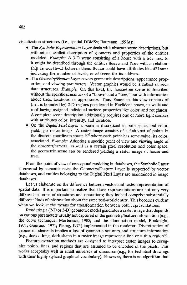
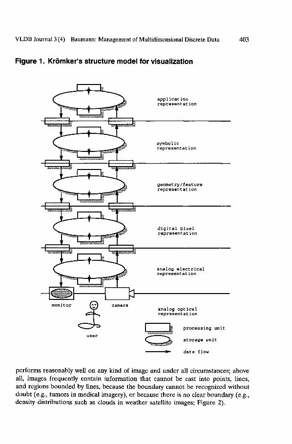


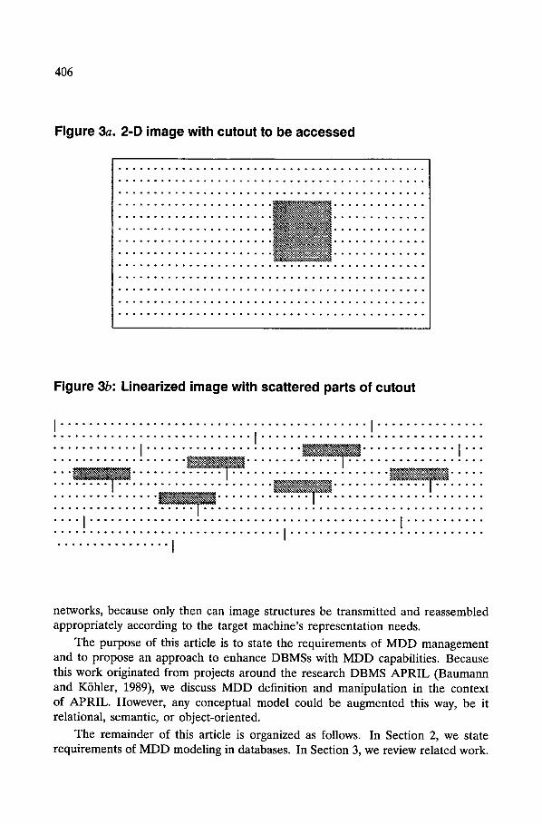


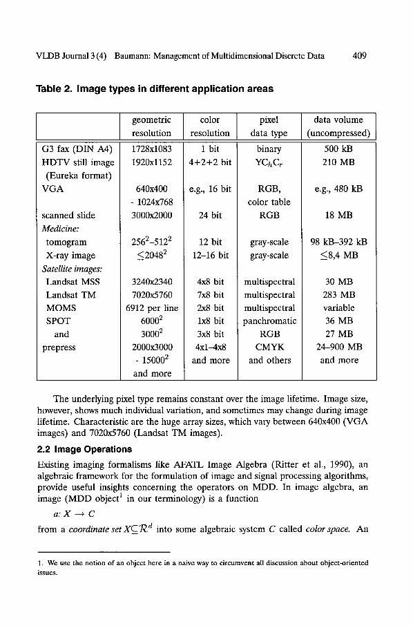


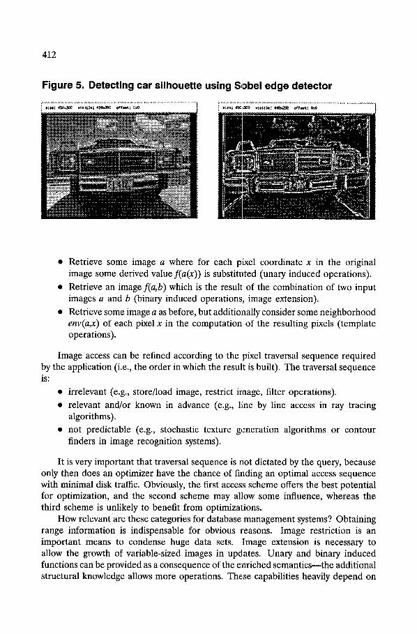

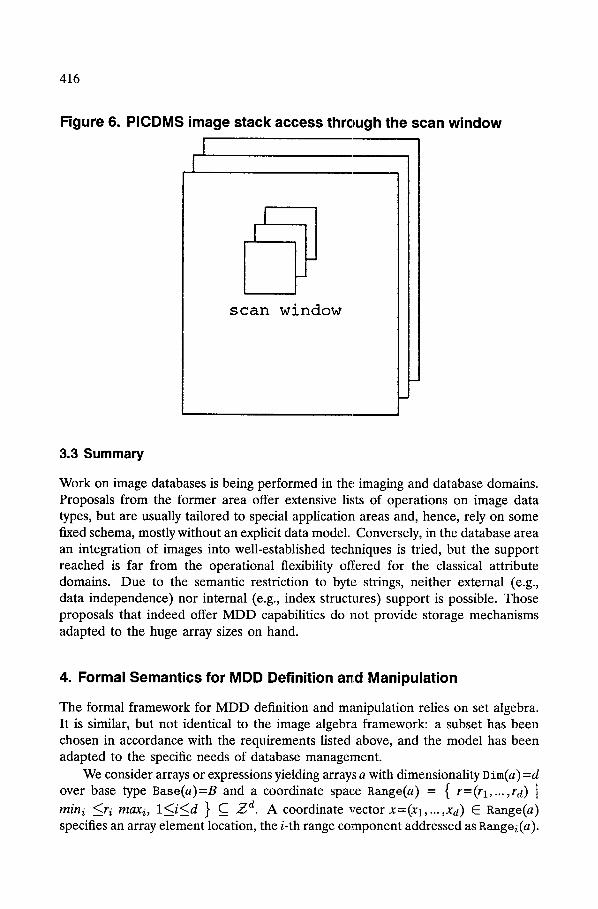


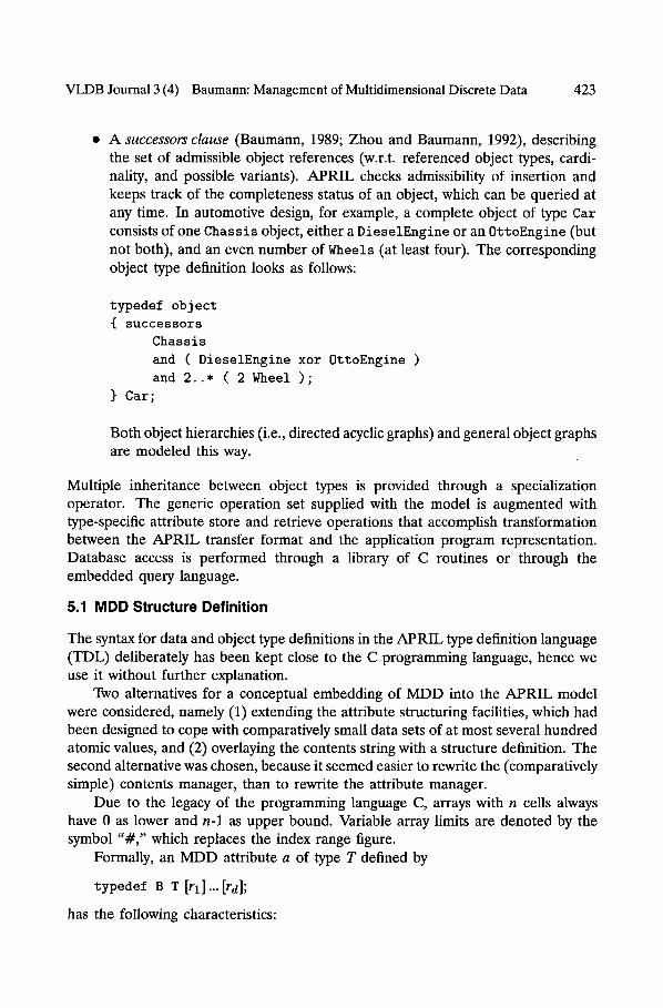


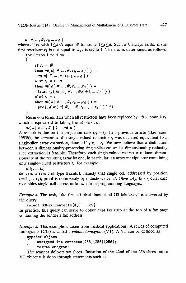


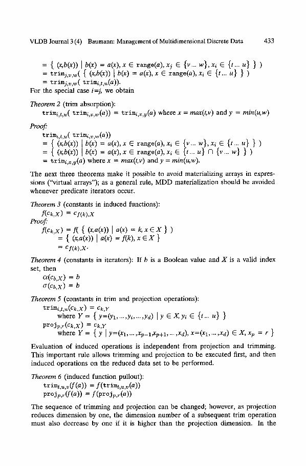
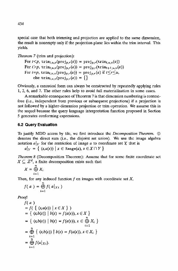

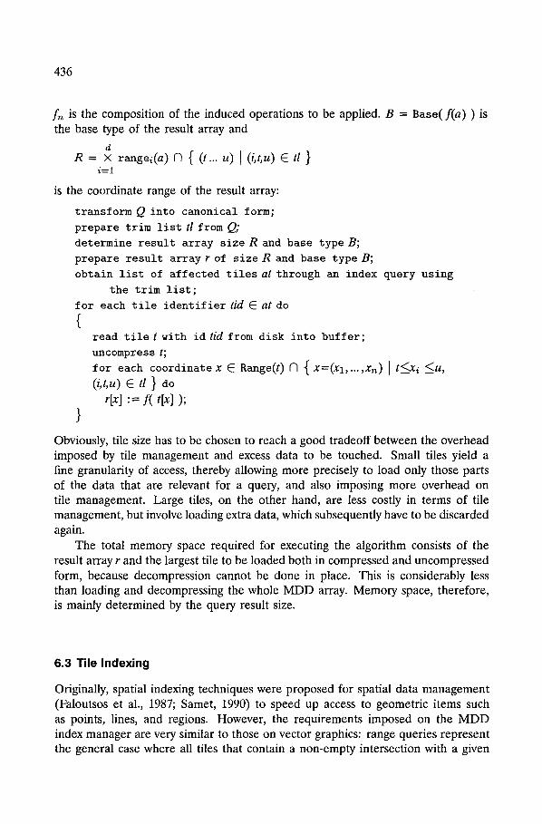


![10-1 Lesson 10 Objectives Chapter 4 [1,2,3,6]: Multidimensional discrete ordinates Chapter 4 [1,2,3,6]: Multidimensional discrete ordinates Multidimensional.](https://static.documents.pub/doc/80x56/5697bff81a28abf838cbf777/10-1-lesson-10-objectives-chapter-4-1236-multidimensional-discrete-ordinates.jpg)


