70
Managerial Economics
| Date post: | 19-Dec-2015 |
| Category: |
Documents |
| View: | 287 times |
| Download: | 7 times |
Managerial Economics

A Definition: The application of mathematical, statistical and decision-science
tools to economic models to solve managerial problems
Some managerial problems:
What product to produce
What price to charge
Where/how to get financing
Where to locate
How to advertise
What method of production to use
Whether or not to invest in new equipment

Managers’ Objectives • Maximizing the value of the firm
(Through profit maximization)
• Alternative objectives:
=>Market share maximization
=>Growth Maximization
=>Maximizing their own benefits
=>Stisfice vs. optimize
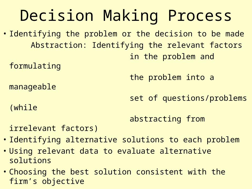
Decision Making Process• Identifying the problem or the decision to be made
Abstraction: Identifying the relevant factors
in the problem and formulating
the problem into a manageable
set of questions/problems (while
abstracting from irrelevant factors)
• Identifying alternative solutions to each problem
• Using relevant data to evaluate alternative solutions
• Choosing the best solution consistent with the firm’s objective
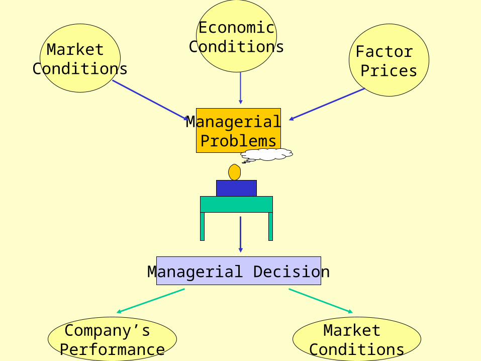
Market Conditions
Factor Prices
Economic Conditions
Managerial Problems
Managerial Decision
Company’s Performance
Market Conditions

Consider the following news headlines:• Gateway cuts jobs: PC maker to trim 15 percent of
staff, expects shortfall in third quarter.
• U.S. consumers lost confidence in August.
• The International Monetary Fund will cut its global economic growth forecast for this year to 2.8 percent.
• Coca-Cola Co., facing a stiff challenge from its arch rival PepsiCo Inc. in the fast-growing alternative drinks market, may be preparing to acquire the Nantucket Nectars line of juice and tea products, analysts said Tuesday.
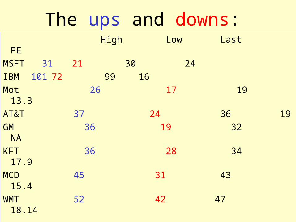
The ups and downs: High Low Last PE
MSFT 31 21 30 24
IBM 101 72 99 16
Mot 26 17 19 13.3
AT&T 37 24 36 19
GM 36 19 32 NA
KFT 36 28 34 17.9
MCD 45 31 43 15.4
WMT 52 42 47 18.14
Macroeconomics, Microeconomics and
and Managerial Decision Making
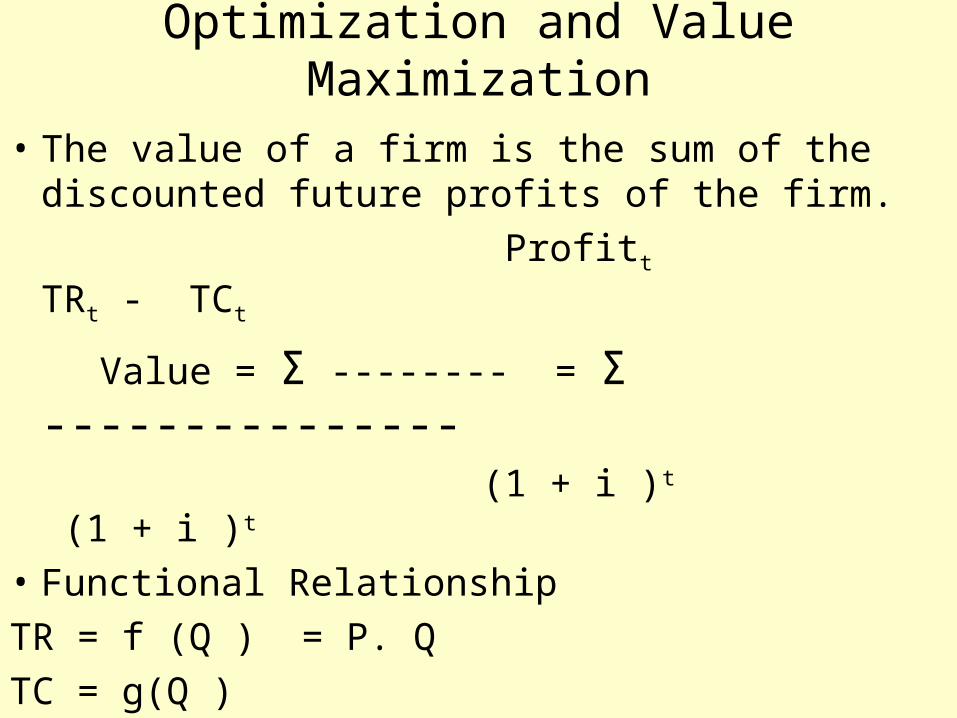
Optimization and Value Maximization
• The value of a firm is the sum of the discounted future profits of the firm.
Profitt TRt - TCt
Value = Σ -------- = Σ --------------- (1 + i )t (1 + i )t
• Functional Relationship
TR = f (Q ) = P. Q
TC = g(Q )
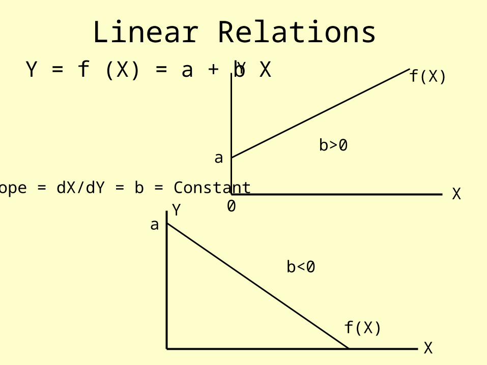
Linear Relations Y = f (X) = a + b X f(X)
X
Y
Slope = dX/dY = b = Constant
f(X)
0
X
Y
b>0
b<0
a
a

Nonlinear Relations • Y = f (x)
• Standard nonlinear forms: Quadratic, Cubic
Y Y
0 0X X

Profit Function • Linear TR
• Quadratic TC
• Quadratic Profit
$
Q
Q
$
TC TR
Profit
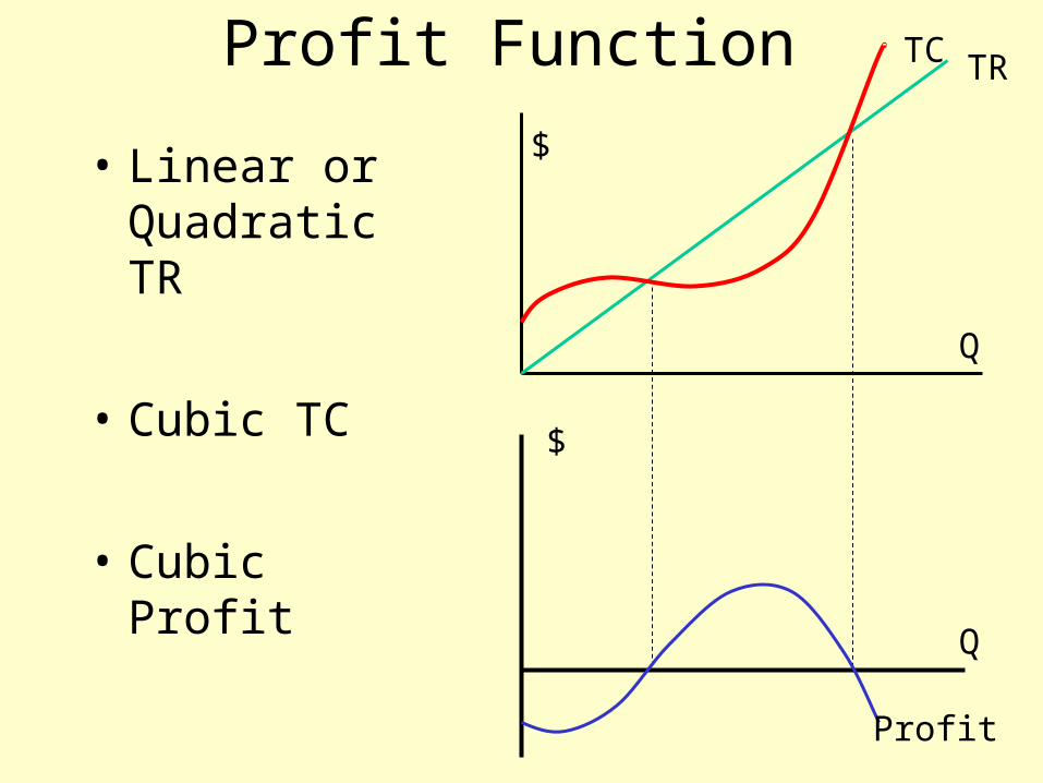
Profit Function
• Linear or Quadratic TR
• Cubic TC
• Cubic Profit
Profit
TR TC
$
$
Q
Q

S
DQ
0
P
P
Q
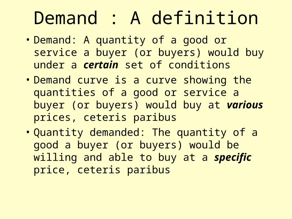
Demand : A definition• Demand: A quantity of a good or service a
buyer (or buyers) would buy under a certain set of conditions
• Demand curve is a curve showing the quantities of a good or service a buyer (or buyers) would buy at various prices, ceteris paribus
• Quantity demanded: The quantity of a good a buyer (or buyers) would be willing and able to buy at a specific price, ceteris paribus
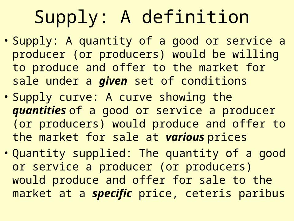
Supply: A definition • Supply: A quantity of a good or service a producer
(or producers) would be willing to produce and offer to the market for sale under a given set of conditions
• Supply curve: A curve showing the quantities of a good or service a producer (or producers) would produce and offer to the market for sale at various prices
• Quantity supplied: The quantity of a good or service a producer (or producers) would produce and offer for sale to the market at a specific price, ceteris paribus

Why do we study supply and demand?
We assume, generally, firms are value maximizers, realizing that the value of a firm is function of its (expected) future profits.
Profit = TR - TC
TR = P . Q
==> What are the factors that determine p and Q?
==> What are the elements determining a firm’s
costs?
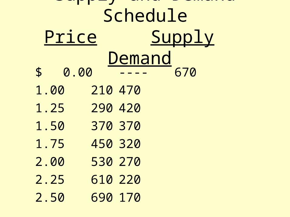
Supply and Demand SchedulePrice Supply Demand
$ 0.00 ---- 670
1.00 210 470
1.25 290 420
1.50 370 370
1.75 450 320
2.00 530 270
2.25 610 220
2.50 690 170

Supply and Demand Equations
• Demand:
Qd = 670 -200 P
P = 3.35 -.005 Qd
• Supply:
Qs = - 110 + 320 P
P = .34375 + .003125 Qs
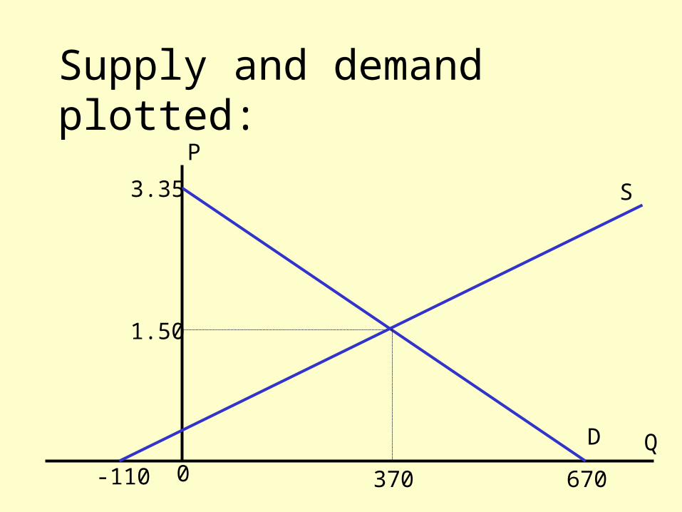
Supply and demand plotted:
3.35
1.50
670
D
-110
S
3700Q
P

An algebraic approach to supply and demand: Qd = f ( Price, Income, X1, X2, ……Xn)
Qd = 20 + .1 Income - 2 Age - 50 Price
Qs = g( Price, W1, W2, ……. Wn )
Qs = -40 - 5 Wage + 30 Price
Income = 2000
Age = 30
Wage = $8

Supply and demand curves
Qd = 20 + .1 Income - 2 Age - 50 Price
($2000) (30)
Qd = 160 - 50P
P = 3.2 - .02 Qd
Qs = -40 - 5 Wage + 30 Price
( $8)
Qs = - 80 + 30 P
P = 2.666 + .0333 Q
Shifts in supply and demand curve:
• A change in any non-price factor in the demand function would result in a shift in the curve: changes in the intercepts.
• A change in any non-price factor in the supply function would result in a shift in the curve: changes in the intercepts.
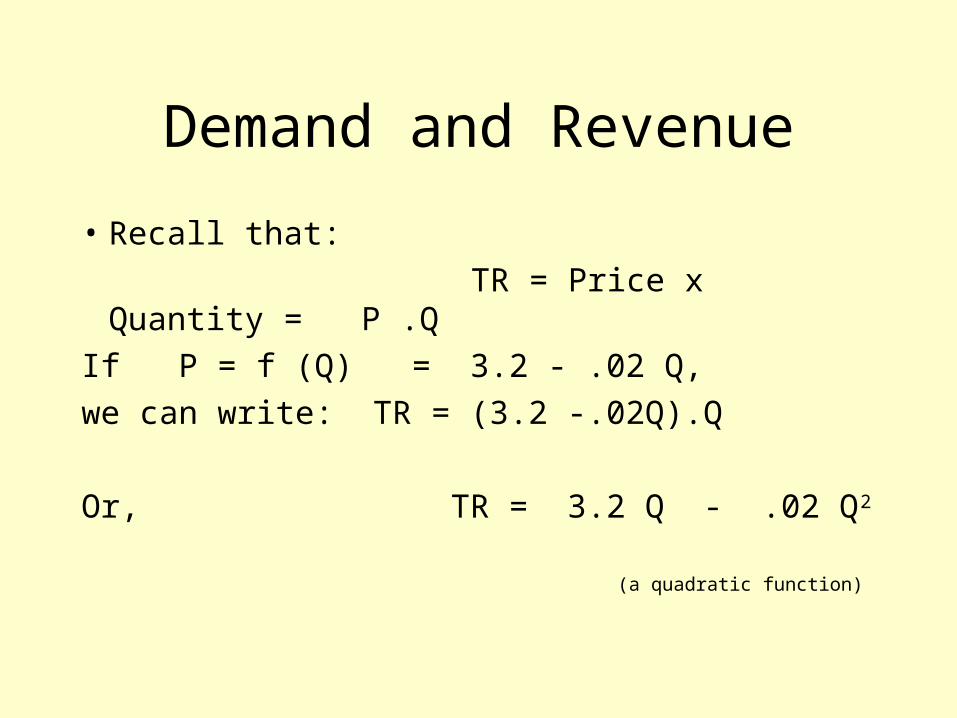
Demand and Revenue
• Recall that:
TR = Price x Quantity = P .Q
If P = f (Q) = 3.2 - .02 Q,
we can write: TR = (3.2 -.02Q).Q
Or, TR = 3.2 Q - .02 Q2
(a quadratic function)
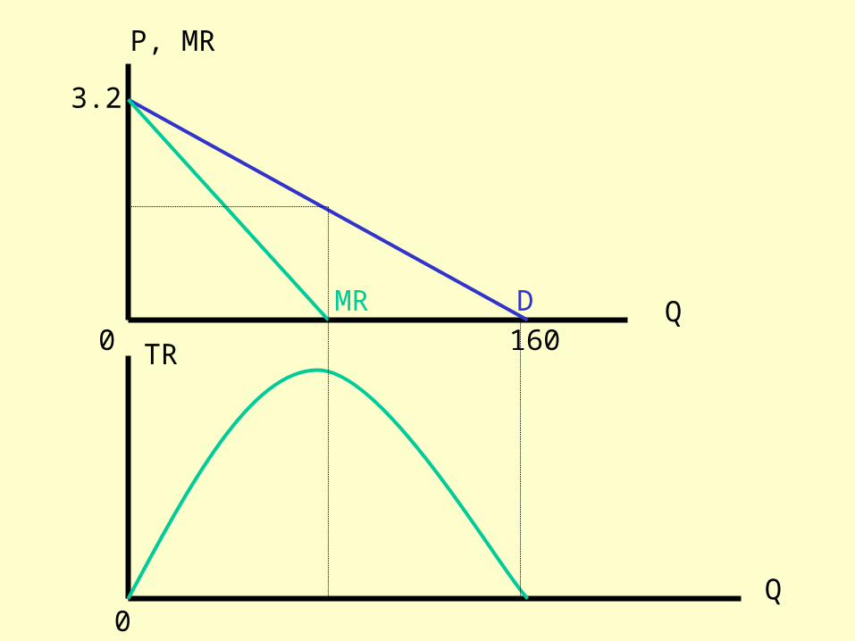
3.2
1600Q
P, MR
D
TR
0Q
MR

The case of a horizontal demand curve:
D
P
0 Q
TR
Q0
TR
Price
TR = P.Q

Marginal versus AverageRecall: TR = P. Q = 3.2 Q - .02 Q2
TR
AR = ------ = 3.2 - .02 Q = P
Q
TR d TR
MR = ------- = ------- = 3.2 - .04 Q
Q d Q
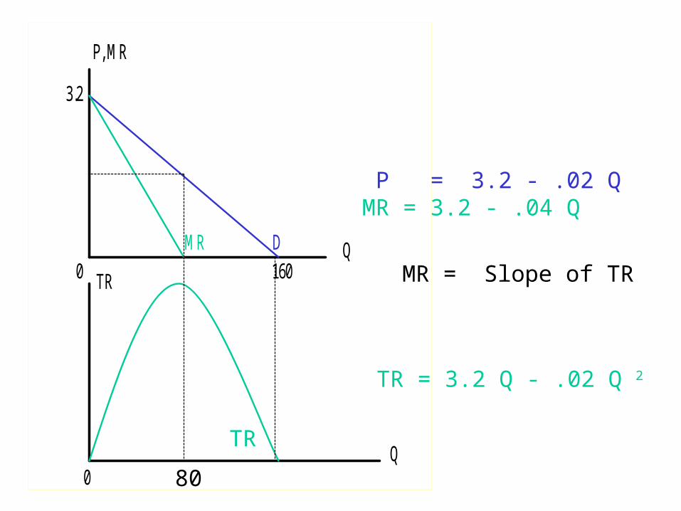
3.2
1600Q
P, MR
D
TR
0Q
MR
P = 3.2 - .02 Q MR = 3.2 - .04 Q
TR = 3.2 Q - .02 Q 2
MR = Slope of TR
80
TR

The case of a horizontal demand curve:
D
P
0 Q
TR
Q0
TR
Price
TR = P.Q
In this case the price, P, is a constant.
TR = P. Q dTR d(P.Q)MR = ------ = --------- = P d Q d Q
==> P = MR
Why is the demand curve generally downward-sloping?
The Consumer theory :
•The indifference curve•The Budget line

The Consumer Theory• The concept of “utility”• Cardinal measurement of utility• Ordinal measurement of utility• Marginal utility• The principle of diminishing marginal utility• Marginal utility and consumer choice• Consumers’ optimizing behavior• The Consumer’s optimizing rule >> the cardinal approach >> the ordinal approach

Utility
The satisfaction or pleasure a consumer derives from the consumption or possession of a good (or service) or an activity (or lack thereof), over a certain span of time.
Note: An economic “bad” is an object, a condition, or an activity that brings on harm or displeasure to a consumer. A consumer derives utility from having an economic “bad” reduced or eliminated.
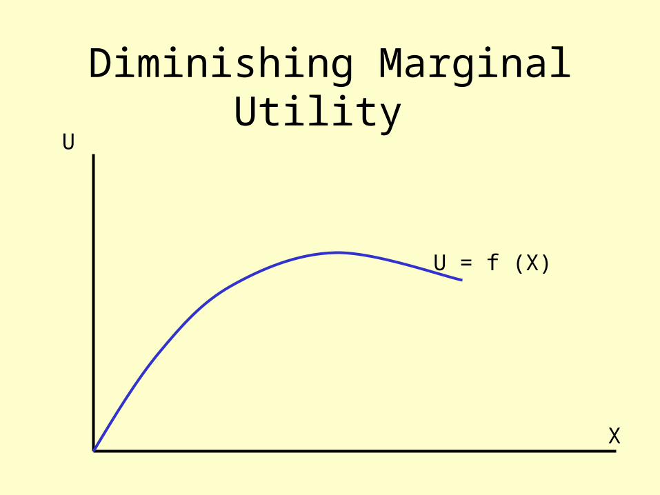
Diminishing Marginal Utility U
X
U = f (X)
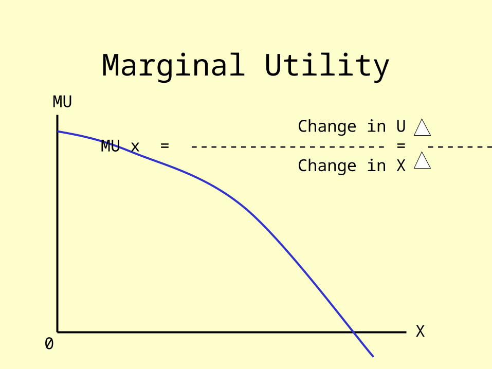
Marginal UtilityMU
X0
Change in U UMU x = -------------------- = ----------- Change in X X

Consumer Choice
Constrained by her income, to maximize her total utility a consumer allocates her income among different goods in such a way that the utility derived from the last dollar spent on each good would be equal to that each of the other goods.

The principle of diminishing marginal utility:
• As a consumer consumes more and more of a good, beyond a certain level, the utility of each additional unit of it (marginal utility) begins to decrease.
• As a consumer consumes more and more of a good, beyond a certain level, each additional unit of that good becomes less dear to him/her
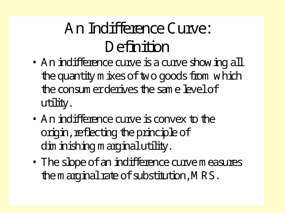
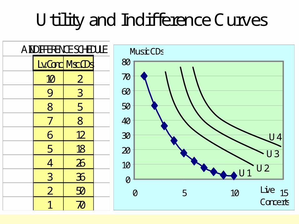
An Indifference Curve:Definition
• An indifference curve is a curve showing all the quantity mixes of two goods from which the consumer derives the same level of utility.
• An indifference curve is convex to the origin, reflecting the principle of diminishing marginal utility.
• The slope of an indifference curve measures the marginal rate of substitution, MRS.
Utility and Indifference Curves
0
10
20
30
40
50
60
70
80
0 5 10 15
Music CDs
Live Concerts
A INDIFFERENCE SCHEDULELv. Conc Msc.CDs
10 29 38 57 86 125 184 263 362 501 70
U1 U2
U3
U4
Properties of an indifference curve
• Generally, negatively sloped, reflecting marginal rate of substitution
• Convex to the origin, reflecting diminishing marginal utility
• Two indifference curves cannot cross
• Special case: a positively sloped indifference curve

Marginal Rate of Substitution
• Definition: The rate at which a consumer is willing to substitute one good for another good while remaining at the same level of satisfaction. That is the amount of good X needed to replace one unit of (lost) good Y to keep the consumer’s level of satisfaction (utility) unchanged.
• MRS = Slope of the indifference curve
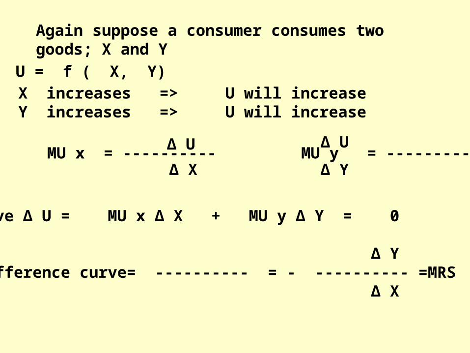
Again suppose a consumer consumes two goods; X and Y
U = f ( X, Y)
As X increases => U will increase As Y increases => U will increase
Recall: MU x = ---------- MU y = ------------
Δ U
Δ X
Δ U
Δ Y
Along any given indifference curve Δ U = MU x Δ X + MU y Δ Y = 0
Δ Y MU x Slope of an indifference curve= ---------- = - ---------- =MRS Δ X MU y
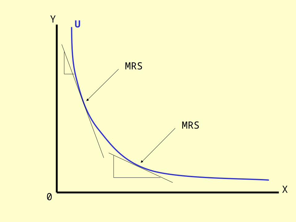
U
0
Y
X
MRS
MRS

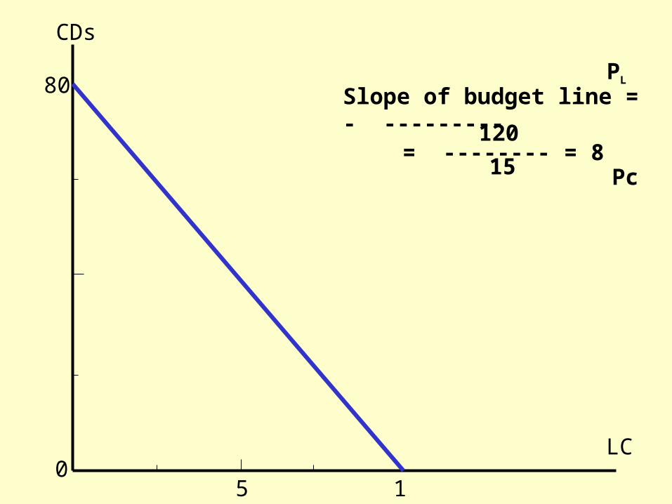
Budget Line
A line showing all combinations of the quantities of two goods a consumer can buy with a given amount of income (budget).
Assuming a consumer is spending all her income on two (symbolic) consumer goods: CDs and live concerts,
Income = Pc . Qc + PL . QL
Pc = 15 , PL = 120 , Income = 1200
CD intercept = 80 LC intercept = 10
CDs
LC
80
1050
Slope of budget line = - --------- Pc
PL
= -------- = 8120
15

CDs
LC
80
1050
Slope of budget line = - --------- Pc
PL
= - -------- = - 8120
15
Pc = 120Pc=240
Pc = 80
= - -------- = -16 240
15
= - -------- = - 5.33 80
15
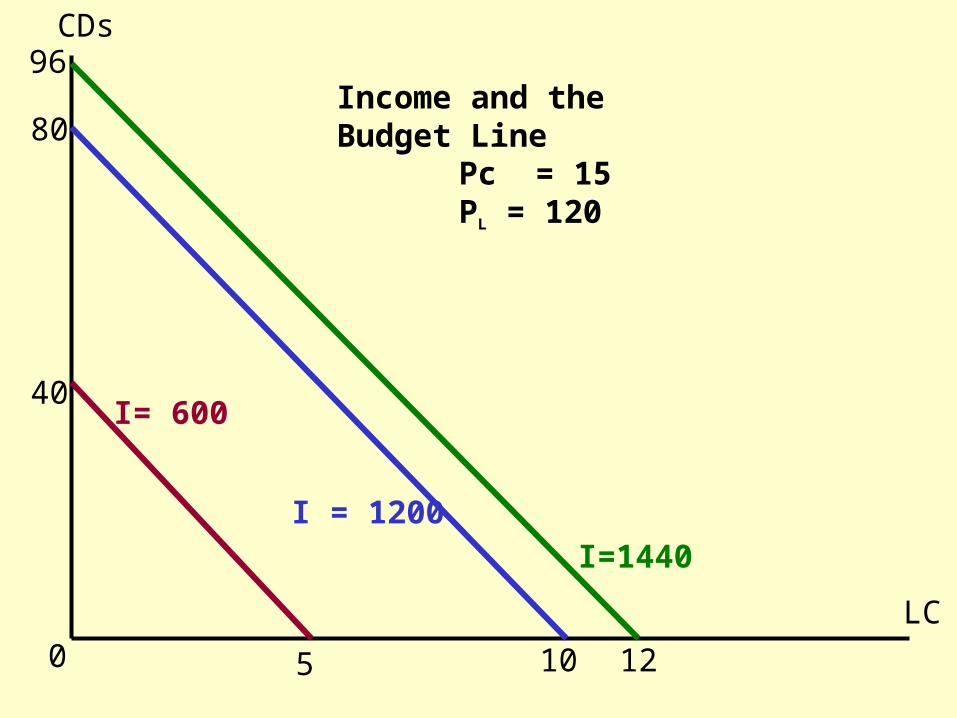
0
LC
CDs
I=1440
I = 1200
I= 600
Income and the Budget Line
105 12
40
80
96
Pc = 15PL = 120
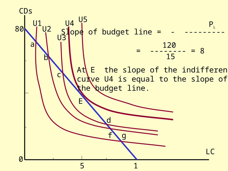
CDs
LC
80
1050
U1U2
U3
U4 U5
E
a
b
c
d
f g
Slope of budget line = - --------- Pc
PL
= -------- = 8120
15
At E the slope of the indifference curve U4 is equal to the slope of the budget line.
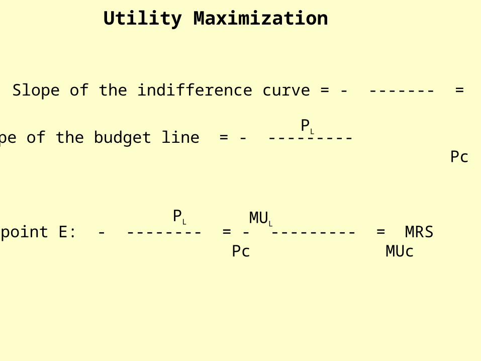
Recall that: MUL
Slope of the indifference curve = - ------- = MRS MUc
Slope of the budget line = - --------- Pc
PL
At point E: - -------- = - --------- = MRS Pc MUc
PL MUL
Utility Maximization

Y
Xo
X1 X2 X3
PX1 > PX2 > PX3
12
3
Demand Curve Derivation
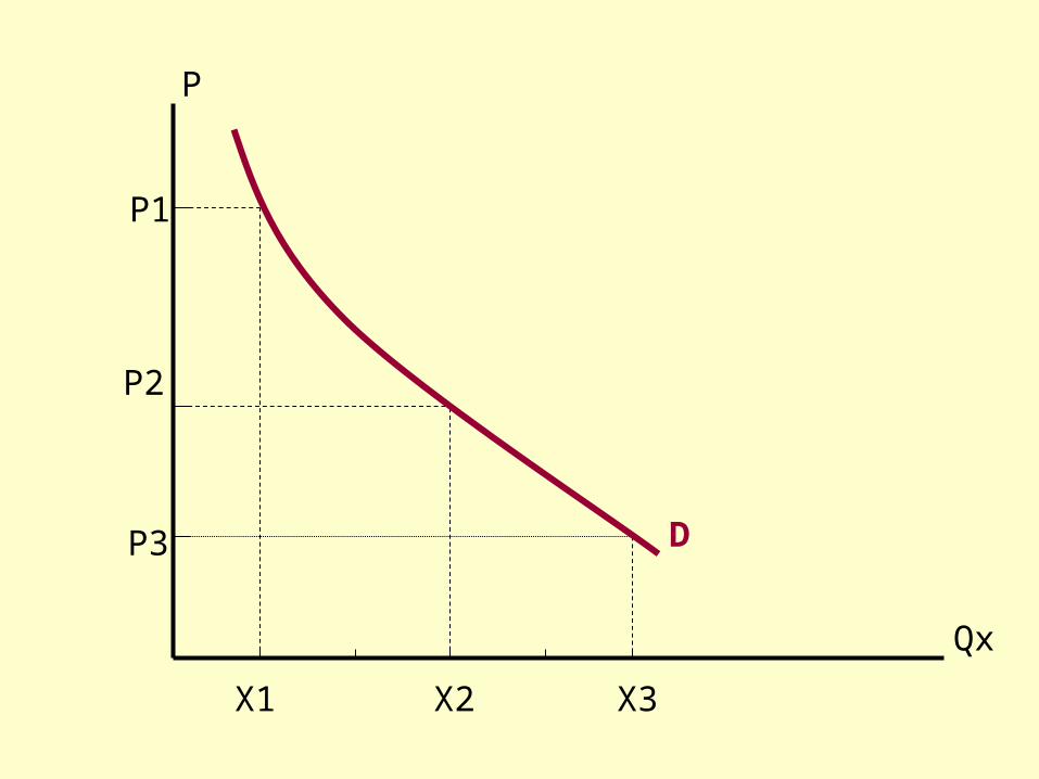
X1 X2 X3
P1
P2
P3
P
Qx
D

Elasticity
A general definition:
Elasticity is a standardized measure of the sensitivity of one (dependent) variable to changes in another variable.
Price elasticity of demand:
A measure of the sensitivity of the quantity demanded a good to changes in the price of that good.
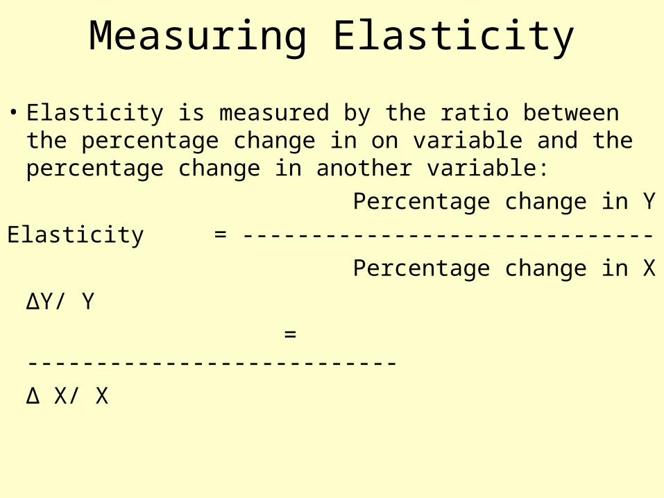
Measuring Elasticity
• Elasticity is measured by the ratio between the percentage change in on variable and the percentage change in another variable:
Percentage change in Y
Elasticity = ------------------------------
Percentage change in X
ΔY/ Y
= ---------------------------
Δ X/ X
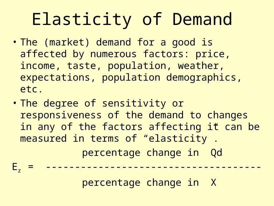
Elasticity of Demand • The (market) demand for a good is affected by
numerous factors: price, income, taste, population, weather, expectations, population demographics, etc.
• The degree of sensitivity or responsiveness of the demand to changes in any of the factors affecting it can be measured in terms of “elasticity”.
percentage change in Qd
Ez = -------------------------------------
percentage change in X

Measuring Elasticity Measuring a change in percentage terms:
Y2 –Y1 Y1 = 80% change in Y = ------------------ Y2 =100
Y1
Y1 –Y2
= -------------------
Y2
Y2 –Y1 Arc % change = -------------------
Y2 +Y1
-----------
2

Measuring Elasticity Change in Qx
-------------------------
Qx1
Ez = --------------------- Change in Z -------------------------
Z1
Change in Qx
--------------------------
Qx1 + Qx2(Arc)Ez = --------------------
Change in Z ------------------------
Z1 + Z2
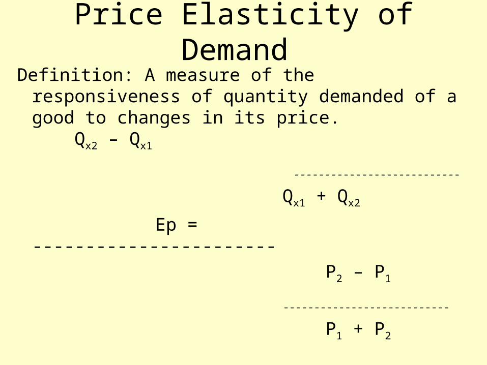
Price Elasticity of Demand
Definition: A measure of the responsiveness of quantity demanded of a good to changes in its price. Qx2 – Qx1
---------------------------
Qx1 + Qx2
Ep = -----------------------
P2 – P1
---------------------------
P1 + P2

Ep (a --- b) = (10/8)/(-2/10) = -6.25
Ep (c ---d ) = (10/80)/(-2/4) = -.25
P
Q
D
ab
cd2
4
8
10
8 18 80 90

Arc (Price) Elasticity
P
Q
D24
Note that if we increasedthe price,
(from 8 to 10 or 2 to 4)
the original P and Q wouldbe 2 and 8 and 18 and90, respectively.
Ep = (-10/18)/(2/8) = -2.22
Ep = (-10/90)/(2/2) = -.11
810
8 18 80 90
a
b
c d

Arc Elasticity
To get the average elasticity between twopoints on a demand curve we take theaverage of the two end points (for bothprice and quantity) and use it as the initialvalue:
Q2-Q1 10
(Q1+Q2) 8+18
Ea = = -3.49
P2-P1 -2
(P1+P2) 10+8
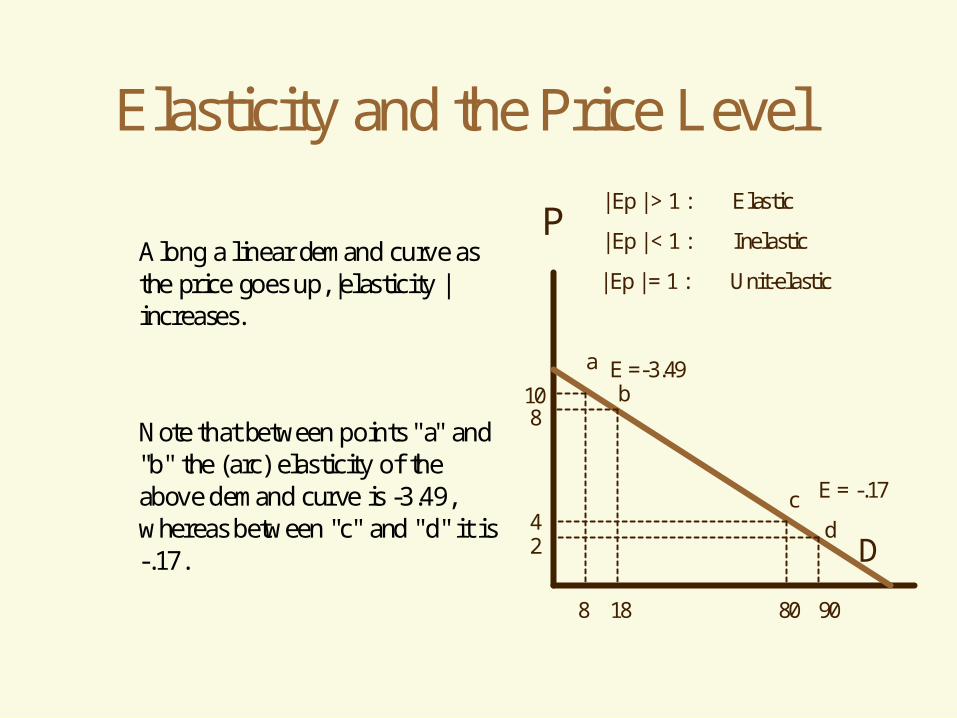
Elasticity and the Price Level
Along a linear demand curve asthe price goes up, |elasticity |increases.
Note that between points "a" and"b" the (arc) elasticity of theabove demand curve is -3.49,whereas between "c" and "d" it is-.17.
P
D
8 18 80 90
a
b
c d
24
810
| Ep | > 1 : Elastic
| Ep | < 1 : Inelastic
| Ep | = 1 : Unit-elastic
E =-3.49
E = -.17
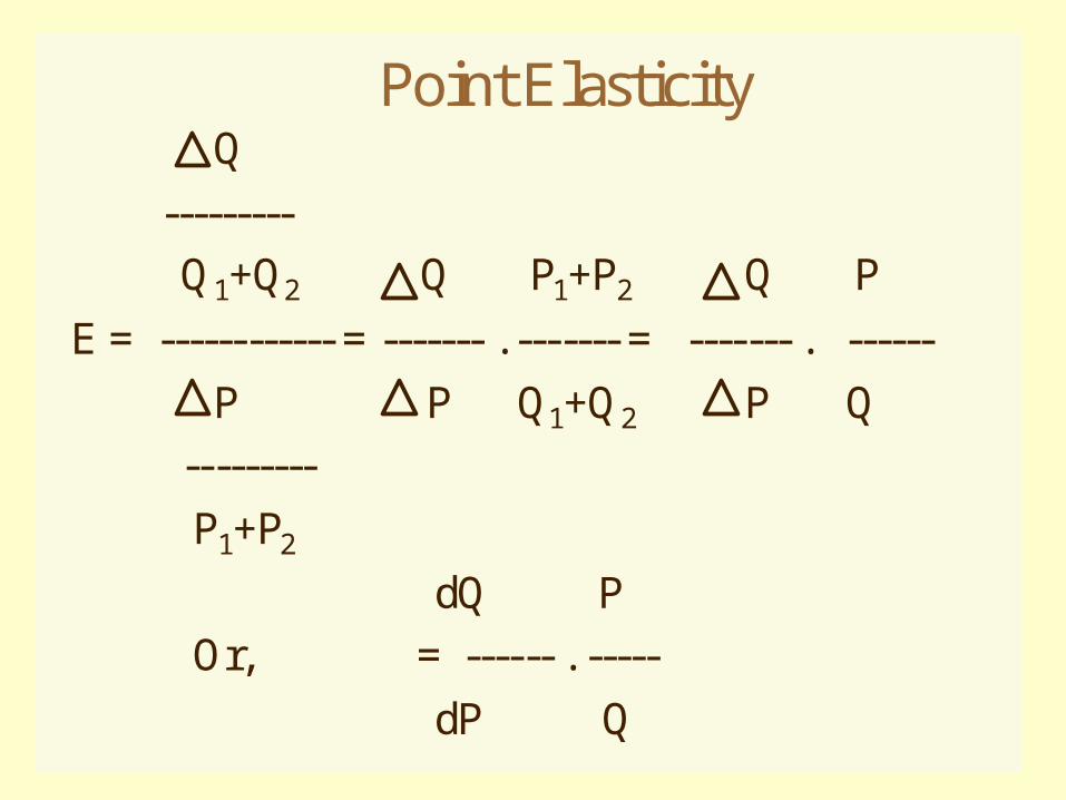
Point Elasticity Q
---------
Q1+Q2 Q P1+P2 Q P
E = ------------ = ------- . ------- = ------- . ------
P P Q1+Q2 P Q
---------
P1+P2
dQ P
Or, = ------ . -----
dP Q
P,MR
Q
Q
TR
0
0
| E | = 1
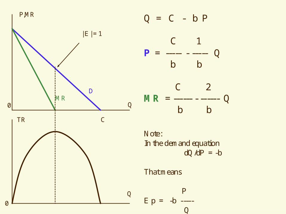
Q = C - b P
C 1P = ----- - ----- Q b b
C 2MR = ------ - ------ Q b b
C
DMR
Note: In the demand equation dQ/dP = -b
That means
PE p = -b ----- Q
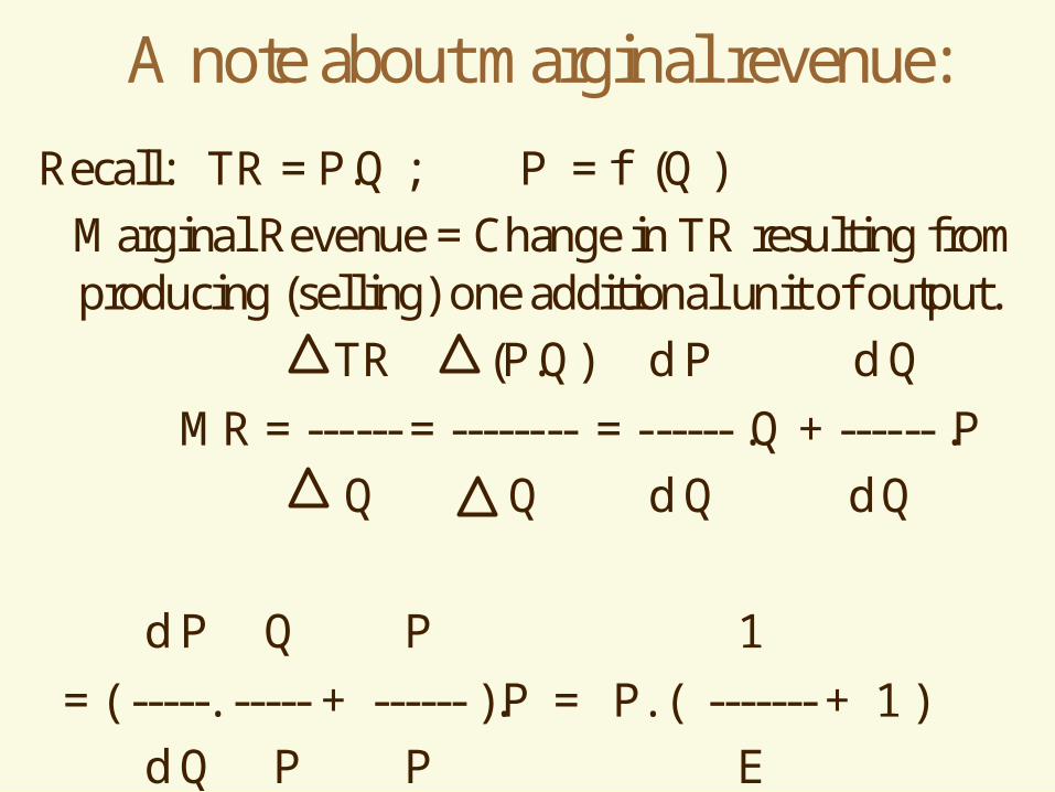
A note about marginal revenue:
Recall: TR = P.Q ; P = f (Q )
Marginal Revenue = Change in TR resulting fromproducing (selling) one additional unit of output.
TR (P.Q) d P d Q
MR = ------ = -------- = ------ .Q + ------ .P
Q Q d Q d Q
d P Q P 1
= ( -----. ----- + ------ ).P = P. ( ------- + 1 )
d Q P P E

0 Q
Q = C - b P
Slope= -1/b
Slope=-2/bD
MR
C
P, MR
dQ ---- = - bd p
dQ P PE = ----- . ----- = -b . ------ d p Q Q
1MR = P. ( 1 + ---- ) E

Important Observations
•When demand is elastic, a decrease in pricewill result is an increase in the revenue(sales).
•When demand is inelastic, a decrease inprice will result is a decrease in the revenue(sales).
•When demand is unit-elastic, an increase(or a decrease) in price will not change therevenue (sales).

What Determines Elasticity
Necessities versus luxuries
Eating at restaurants
Groceries
Availability of substitutes
Chicken versus beef
How much of our income a good takes
Salt versus Nike sneakers
The passage of time
Other Elasticity Measures
Recall: “Elasticity” is a (standard) measure ofthe degree of sensitivity ( or responsiveness) ofone variable to changes in another variable.
Income Elasticity: a measure of the degree ofsensitivity of demand for a good (or service) tochanges in consumers’ (buyers’) income
Cross Price Elasticity: a measure of the degreeof sensitivity of demand for a good (or service)to changes in the price of another good orservice

Income Elasticity of Demand
A measure of the degree of responsivenessof demand (for a good) to a change inincome, ceteris paribus.
(Shift of the demand curve)
Q2-Q1
Q2+Q1 d Q I
EI = = or = ------ . ------
I2-I1 d I Q
I1+I2
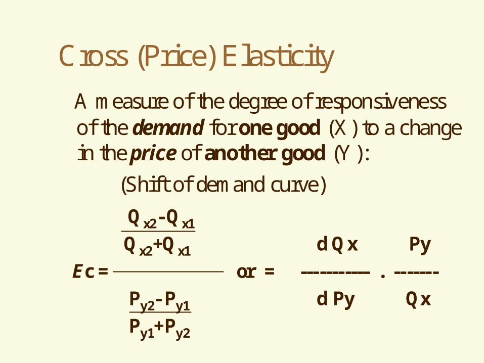
Cross (Price) Elasticity
A measure of the degree of responsivenessof the demand for one good (X) to a changein the price of another good (Y):
(Shift of demand curve)
Qx2- Qx1
Qx2+Qx1 d Qx Py
Ec = or = ----------- . -------
Py2- Py1 d Py Qx
Py1+Py2

Qd = 200 - 2 P + .05 I + .5 W + .5 Pc
P = 95, I = 1000, W = 80, Pc = 200
==> Qd = 200
Ep = - 2 (95/200) = -.95
EI = .05 (1000/200) = .25
Ew = .5 (80/200) = .2
Epc = .5(200/200)= .5
An example:


