SAND2011-1866C

Managing Complexity in Simulation-Based Uncertainty Quantification

B i M Ad

Based Uncertainty Quantification

Brian M. Adamswith Michael S. Eldred and Laura P. Swiler

Workshop on Future Directionsin Applied Mathematics

March 10, 2011Raleigh, NC

Sandia National Laboratories is a multi-program laboratory managed and operated by Sandia Corporation, a wholly owned subsidiary of Lockheed Martin Corporation, for the U.S. Department of Energy’s

National Nuclear Security Administration under contract DE-AC04-94AL85000.

Outline

• Research group goal: general-purpose uncertaintyResearch group goal: general purpose uncertainty quantification (UQ) algorithms and software applicable to expensive or otherwise challenging computational models.

• Motivation for uncertainty quantification (UQ); characterizing uncertaintiesg

• Accessible introduction to UQ methods, challenges, someadvancesCh ll i i t l d lti h i d• Challenging environments: coupled multi-physics, random fields, etc.

2

Insight from Computational SimulationComputational Simulation

Systems of systems analysis: multi-scale,analysis: multi scale, multi-phenomenon

Micro-electro-mechanical systems (MEMS): quasi- Joint mechanics: system-level systems (MEMS): quasi

static nonlinear elasticity, process modeling

yFEA for component

assessment

Electrical circuits: networks, PDEs, differential algebraic

equations (DAEs), E&M

dHurricane Katrina: weather,

logistics, economics, ghuman behaviorEarth penetrator: nonlinear

PDEs with contact, transient analysis, material modeling

V&V, UQ, and Model FidelitySupport Credible SimulationSupport Credible Simulation

Insight, prediction, and risk-informed decision-making require credibility for intended application

non-

Bill Oberkampf

non-deterministic element

Uncertainties in Simulation and ValidationSimulation and Validation

A few uncertainties affecting computational model output/results:• physics/science parameters• statistical variation,

inherent randomness 4.55

Final Temperature Values

T tM d l• model form / accuracy• material properties• manufacturing quality 1

1.52

2.53

3.54

% in

Bin

Test Data

Model Data

• manufacturing quality• operating environment,

interferencei iti l b d diti f i

00.5

Temperature [deg C]

• initial, boundary conditions; forcing• geometry / structure / connectivity• experimental error (measurement error, measurement bias)p ( )• numerical accuracy (mesh, solvers); approximation error• human reliability, subjective judgment, linguistic imprecision

Th ff t f th d l t t h ld b i t l tThe effect of these on model outputs should be integral to an analyst’s deliverable: best estimate PLUS uncertainty!

Categories of Uncertainty

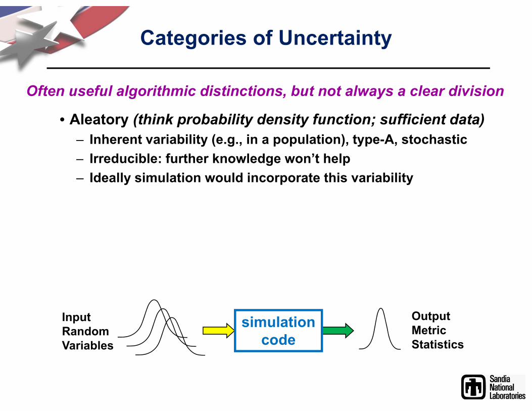
Often useful algorithmic distinctions, but not always a clear division

• Aleatory (think probability density function; sufficient data)– Inherent variability (e.g., in a population), type-A, stochastic

I d ibl f th k l d ’t h l– Irreducible: further knowledge won’t help– Ideally simulation would incorporate this variability

InputRandomVariables

OutputMetricStatistics

simulationcode

Categories of Uncertainty

Often useful algorithmic distinctions, but not always a clear division

• Aleatory (think probability density function; sufficient data)– Inherent variability (e.g., in a population), type-A, stochastic

I d ibl f th k l d ’t h l– Irreducible: further knowledge won’t help– Ideally simulation would incorporate this variability

• Epistemic (e.g., bounded intervals or unknown distro parm)p ( g p )– Subjective, type-B, state of knowledge uncertainty– Reducible: more data or information, would make uncertainty

estimation more preciseestimation more precise– Fixed value in simulation, e.g., elastic modulus,

but not well known[ ]

simulationcode

[ ][ ]

[ ][ ]

InputIntervals

[ ][ ]

[ ]OutputIntervals

[ ] [ ]

Uncertainty Quantification

• Identify and characterize uncertain variables (may not be normal, uniform)• Forward propagate: quantify the effect that (potentially correlated)

uncertain (nondeterministic) input variables have on model output:

Input Variables u(physics parameters, geometry, initial and b d diti )

ComputationalModel

Variable PerformanceMeasures f(u)boundary conditions) Measures f(u)

(possibly given distributions)(here assumed a black-box)

Potential Goals:• based on uncertain inputs, determine variance of outputs and probabilities

of failure (reliability metrics)( y )• validation: is the model sufficient for the intended application?• quantification of margins and uncertainties (QMU): how close are

uncertainty-aware code predictions to performance expectations or limits?uncertainty-aware code predictions to performance expectations or limits?• quantify uncertainty when using calibrated model to predict

Thermal Uncertainty Quantification

• Device subject to heating (experiment or computational simulation)p )

• Uncertainty in composition/ environment (thermal conductivity, density, boundary), parameterized bydensity, boundary), parameterized by u1, …, uN

• Response temperature f(u)=T(u1, …, uN)calculated by heat transfer codecalculated by heat transfer code

Given distributions of u1,…,uN, UQ methods calculate statistical info on outputs:

Final Temperature Valuesstatistical info on outputs:• Mean(T), StdDev(T), Probability(T ≥ Tcritical)

P b bilit di t ib ti f33.5

44.5

5

n • Probability distribution of temperatures• Correlations (trends) and

iti it f t t0.51

1.52

2.53

% in

Bin

sensitivity of temperature030 36 42 48 54 60 66 72 78 84

Temperature [deg C]

Black-box UQ Workhorse: Random Sampling MethodsRandom Sampling Methods

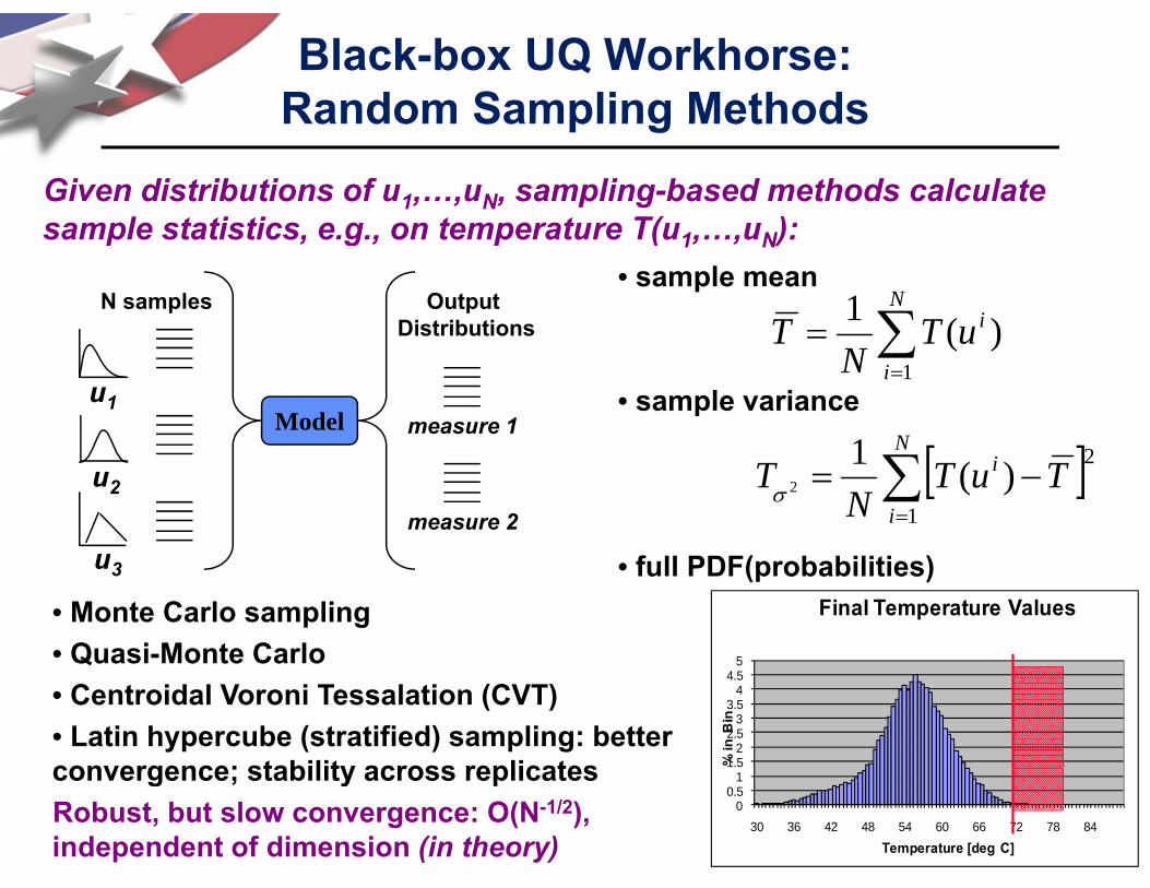
Given distributions of u1,…,uN, sampling-based methods calculate sample statistics e g on temperature T(u u ):

• sample meansample statistics, e.g., on temperature T(u1,…,uN):

Output Distributions

N samples

N

iuTT )(1

• sample variancemeasure 1Model

u1

i

uTN

T1

)(

N1

measure 2

u2

N

i

i TuTN

T1

2)(12

• full PDF(probabilities)

5

Final Temperature Values

u3

• Monte Carlo sampling• Quasi-Monte Carlo

1.52

2.53

3.54

4.55

% in

Bin

Quasi Monte Carlo• Centroidal Voroni Tessalation (CVT)• Latin hypercube (stratified) sampling: better convergence; stability across replicates

00.5

1

30 36 42 48 54 60 66 72 78 84

Temperature [deg C]

convergence; stability across replicatesRobust, but slow convergence: O(N-1/2), independent of dimension (in theory)

Challenges: Simulation-based UQ

• Similar to optimization for simulation-based engineeringN d t ti ti f f ti f P b[ f > f ]• Need statistics of response function f, e.g., µf, f, Prob[ f > fcritical]

• Characteristics/issues:• input parameters characterized by

PDFs or intervalsPDFs or intervals• no explicit function for f(x1,x2)• expensive to evaluate f(x1,x2) (may

1.0

f(x1, x2)fail; limited number of samples)

• noisy, non-smooth, multi-modal• dimension of parameter space

0 40.60.8

p p• complex, coupled systems• evaluate small probabilities

0.00.20.4

0 4

0.20.4

0 6

UQ in DAKOTA attempts to mitigate: a mix of statistics, nonlinear optimization, numerical integration and surrogate modeling enables0.4

0.60.8

1.0 x 1

0.60.8

1.01.2

x2

integration, and surrogate modeling enables robust and efficient UQ methods.

Random Sampling forCoupled SystemsCoupled Systems

• Sampling: not the most efficient UQ methodH t i l t d t t t t• However, easy to implement and transparent to trace sample realizations through complex multi-code UQ studies

Additi l I t

Input Distributions Si l ti

Additional Inputsfor Simulation 2

Output DistributionsN samples of X

N realizations

Simulation Model 2

Simulation Model 1

N realizationsof f(X)

Simulation Measure 1Model 3

Measure 2Additional Inputs for Simulation 3

Challenge: Calculating Potentially Small Probability of FailurePotentially Small Probability of Failure

• Given uncertainty in materials, geometry, and environment, how to determine likelihood of failure:environment, how to determine likelihood of failure: Probability(T ≥ Tcritical)?

• Perform 10,000 LHS samples and count how many exceed threshold;

TTcriticalexceed threshold; (better) perform adaptive importance sampling

Mean value: make a linearity (and possibly normality) assumption and project;

t f t ith

Reliability: directly determine input variables which give rise to failure behaviors by solving an

ti i ti bl f tgreat for many parameters with efficient derivatives!

optimization problem for a most probable point (MPP) of failure

Tuuminimize)( uT T

All th l li ti i ti

criticalTT(u)uu subject to

minimize)()(),(

)(

uj

ui j i

uT

uT

dudg

dudgjiCov

All the usual nonlinear optimizationtricks apply…

Efficient Global Reliability Analysis:GP Surrogate + MMAIS (B.J. Bichon)g ( )

• Apply an EGO-like method to the equality-constrained optimization problem• In EGRA, an expected feasibility function balances exploration with localIn EGRA, an expected feasibility function balances exploration with local

search near the failure boundary to refine the GP• Cost competitive with best MPP search methods, yet better probability of

failure estimates; addresses nonlinear and multimodal challengesfailure estimates; addresses nonlinear and multimodal challengesGaussian process model (level curves) of reliability limit state with

10 samples 28 samples

exploit

failure region

exploresafe

region exploreg

Challenge: Dimension Selection and ResolutionDimension Selection and Resolution

• Open (impossible?) challenge: “needle in a haystack” UQ problems (local features without global trends e gproblems (local features without global trends, e.g., interatomic potential minimization or rare AND isolated event); perhaps a challenging exhaustive global

ti i ti bl t ti l f i d loptimization problem; not practical for expensive models

• Tractable challenge: identify and resolve uncertainties in g ycrucial input dimensions, e.g., reduce from O(1000) to O(10) key parameters

advance screening (global sensitivity) then UQ– advance screening (global sensitivity), then UQ– online, adaptive methods for stochastic expansions– leverage gradient information if available cheaplyg g p y

• While similar for polynomial chaos and interpolation-based t h ti ll ti ( d th ti ll i l tstochastic collocation (and they are essentially equivalent

in practice), examples here are for PCE.15

Generalized Polynomial Chaos Expansions (PCE)

Approximate response with Galerkin projection using multivariate orthogonal polynomial basis functions defined over standard

Chaos Expansions (PCE)

g p yrandom variables

• Intrusive or non-intrusiveR(ξ) ≈ f(u)

Intrusive or non intrusive• Wiener-Askey Generalized PCE: optimal basis selection leads to

exponential convergence of statistics

• Can also numerically generate basis orthogonal to empirical data (PDF/histogram)

Forming PCE/SC Expansions(for PCE, using Ri to estimate αj)(for PCE, using R to estimate αj)

Random sampling: PCE Tensor-product quadrature: PCE/SC

Expectation (sampling):– Sample w/i distribution of x– Compute expected value of

product of R and each Y

Tensor product of 1-D integration rules, e.g.,Gaussian quadrature

product of R and each YjLinear regression (“point collocation”):

Smolyak Sparse Grid: PCE/SC Cubature: PCEy pStroud and extensions (Xiu, Cools):optimal multidimensional integration rules

TPQ

SS

G

Adaptive Approaches:Emphasize Key DimensionsEmphasize Key Dimensions

• Uniform p-refinementUniform p refinement– Stabilize 2-norm of covariance

• Adaptive p-refinement ~LHS

– Estimate main effects/VBD to guide• h-adaptive: identify important

regions and address discontinuities

SSG TPQ

regions and address discontinuities• h/p-adaptive: p for performance;

h for robustness

Anisotropic index sets Anisotropic Gauss-Hermite

18

Comparison of PCE/SC ApproachesPCE/SC Approaches

19

Extend Scalability through Derivative EnhancementDerivative Enhancement

• Leverage more data at each model evaluation (typically N+1 forevaluation (typically N+1 for gradients)

• PCE: linear regression with derivatives (simply additionalderivatives (simply additional equations)

• SC: gradient-enhanced interpolants(more challenging) via cubic Lagrange(more challenging) via cubic Lagrange splines or Hermite polynomials

• EGRA: gradient-enhanced Kriging/co-Kriging Interpolates function valuesKriging. Interpolates function values and gradients

Interval Estimation Approach(Probability Bounds Analysis)(Probability Bounds Analysis)

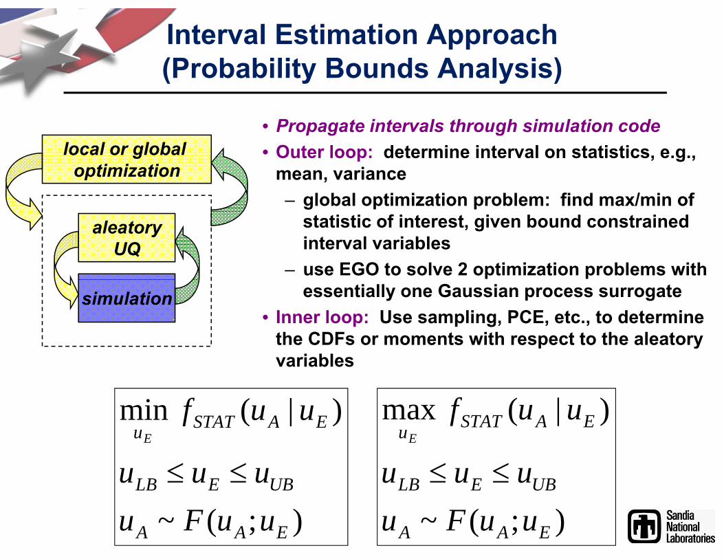
• Propagate intervals through simulation codel l l b l • Outer loop: determine interval on statistics, e.g.,

mean, variance– global optimization problem: find max/min of

local or global optimization

statistic of interest, given bound constrained interval variables

– use EGO to solve 2 optimization problems with

aleatoryUQ

essentially one Gaussian process surrogate• Inner loop: Use sampling, PCE, etc., to determine

the CDFs or moments with respect to the aleatory

simulation

p yvariables

)|(min AS A uuf )|(max EASTAT uuf)|(min

UBELB

EASTATu

uuu

uufE

)|(max

UBELB

EASTATu

uuu

uufE

);(~ EAA

UBELB

uuFu );(~ EAA

UBELB

uuFu

Interval Analysis can beTractable for Large-Scale AppsTractable for Large Scale Apps

Multiple cells within DSTEwithin DSTE

C t ti b d ith 10 100 l l ti

25

Converge to more conservative bounds with 10—100x less evaluations

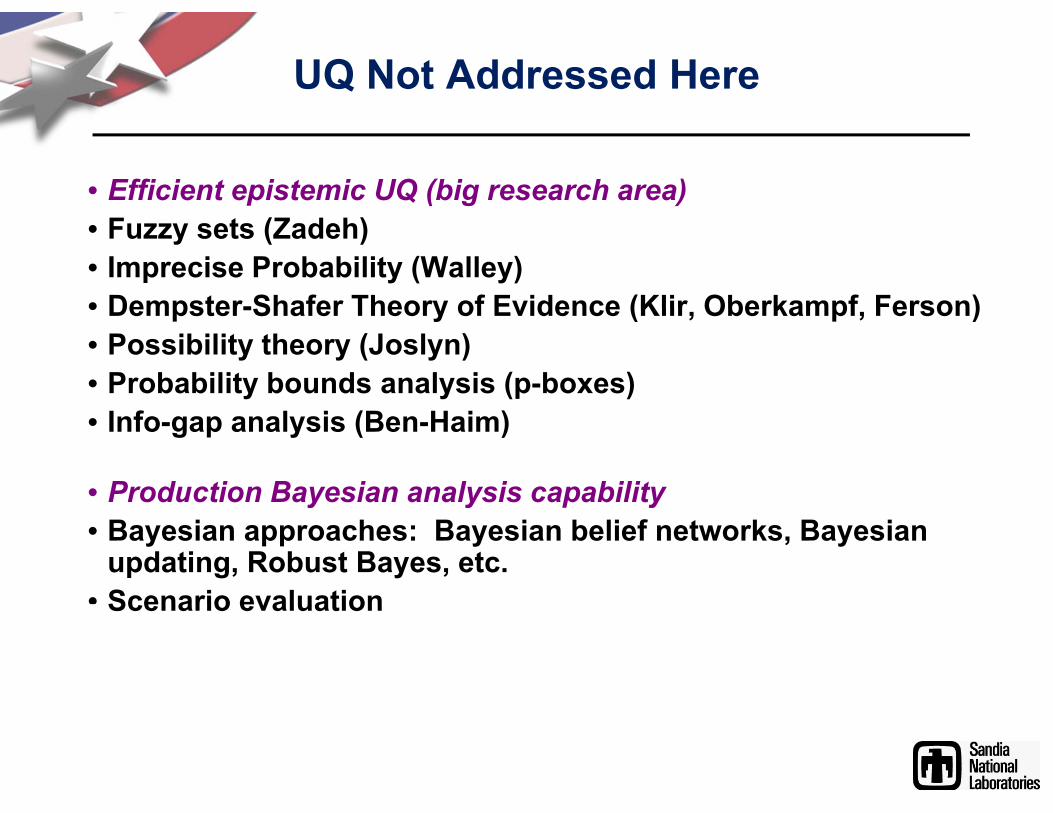
UQ Not Addressed Here

• Efficient epistemic UQ (big research area)• Fuzzy sets (Zadeh)• Imprecise Probability (Walley)• Dempster-Shafer Theory of Evidence (Klir Oberkampf Ferson)• Dempster-Shafer Theory of Evidence (Klir, Oberkampf, Ferson)• Possibility theory (Joslyn)• Probability bounds analysis (p-boxes)• Info-gap analysis (Ben-Haim)

• Production Bayesian analysis capabilityy y p y• Bayesian approaches: Bayesian belief networks, Bayesian

updating, Robust Bayes, etc.• Scenario evaluationScenario evaluation

Checkpoint

• UQ algorithm efficiency is crucial when combiningUQ algorithm efficiency is crucial when combining algorithms, e.g, for optimization under uncertainty, robust optimization, or nested uncertainty analysisS dd hi h di i lit ith d ti• Some progress: address high dimensionality with adaptive methods and derivative-enhancement

• Address expense and nonlinearity in part through global p y p g gsurrogate models

• To conclude: a few examples of li– coupling

– complex systems

27

UQ for Coupled Multi-Physics

• Can we efficiently propagate UQ across scales/disciplines?• Naively wrapping multi physics with UQ often too costly• Naively wrapping multi-physics with UQ often too costly• Can we invert loops and perform multi-physics analysis on

UQ-enriched simulations (couple based on scalar statistics, random fields, stochastic processes)?

28Source: CASL (DOE Energy Innovation Hub)

Multi-Physics, Multi-Fidelity, Heterogeneous UQHeterogeneous UQ

• Component-level uncertainty propagation via stochastic expansionsp

• Stochastic dimension reduction at component interfaces

• Strongly coupled solver technology for

L fid lit N t k Pl t M d l

g y p gycoupled stochastic problems

• Stochastic upscaling for low-fidelity models• Stochastic sensitivities with respect to

d Sc

hmid

t, ct

Low-fidelity Network Plant Model

Component 1

Stochastic sensitivities with respect to system components

s co

urte

sy: R

odB

RIS

C p

roje

c

Component 2

Gra

phic

s

High-fidelity Multi-physics

Nonlinear eliminationEquations Newton Step

High-fidelity Multi-physics Component Model (Core)

Electrical Modeling Complexity

Circuit Board

Large Digital CircuitASIC: 1000s to millions of devices

simulation g g

(e.g., ASIC)Sub-circuit (analog)

sub-circuit: 10s to 100s of devices

millions of devices time grow

s

Single Device

s exponentia

• simple devices: 1 parameter,

device: 1 to 100s of params

• complex devices: many parameters, some

ally

(G. Gray, M. M-C, SNL)

p ptypically physical and measurable

• e.g., resistor @ 100Ω +/- 1%

p y p ,physical, others “extracted” (calibrated)

• multiple modes of operation• e.g., zener diode: 30 parameters, 3 bias

• resistors, capacitors, inductors, voltage sources

g pstates; many transistor models (forward, reverse, breakdown modes)

Hierarchical/Network Structure

• How can we exploit electrical systems’ natural hierarchy or network structure?hierarchy or network structure?

• How does uncertainty propagate? Sufficient to propagate variance?

system level(performance metrics)

system level(performance metrics)

p p g• Use surrogate/macro-models as glue between

levels?circuit level

(circuit characteristics)circuit level

(circuit characteristics)

• Can approaches be implemented generically to apply to any circuit implemented in Xyce? device level

(model parameters)device level

(model parameters)

process level(physical parameters)

process level(physical parameters)

Challenge: UQ forFluid-Structure InteractionsFluid Structure Interactions

• Atmospheric entry vehicles are subject to turbulent flow, complex chemical reactions thermal and pressure loadscomplex chemical reactions, thermal and pressure loads.

• Example goal: assess uncertainty in loads imposed on structures without running costly CFD over many scenarios (typically can’t afford full coupling).

• Need: random field characterization of uncertainty from CFD and efficient way to assess effect on structuralCFD and efficient way to assess effect on structural dynamics.

32

NASA (public domain)

FSI: Nuclear ReactorGrid-to-rod Fretting FailureGrid to rod Fretting Failure

• Clad failure can result from rod-spring interactions Spacer grid cell

– Induced by flow vibration – Amplified by irradiation-induced grid

spacer growth and spring relaxation1 Fuel

spacer growth and spring relaxation• Power uprates and burnup increase

potential for fretting failures (leading cause of fuel failures in PWRs) 2 Fuelcause of fuel failures in PWRs)

• Ideally: High-fidelity, fluid structural interaction tool to predict uncertaintyin gap turbulent flow excitation rod

2 Fuel

in gap, turbulent flow excitation, rod vibration and wear Fuel3

Sources: CASL DOE Energy Innovation Hub,Roger Lu, Westinghouse

Possible Research Directions

GOAL: Advanced efficient, robust, accurate UQ methods for validation, extrapolation, and risk-informed decisions with , p ,expensive computational models

• Efficient adaptive polynomial chaos techniquesEfficient, adaptive polynomial chaos techniques• UQ and surrogate approaches for mixed-integer, higher-order

moments, tail statisticsH t ll t i t• How to allocate margin across a system

• Stochastic processes and random fields• Epistemic UQ approaches and alternative frames• All the above in multi-level (system and hierarchical) UQ contexts

To contribute, understand: (1) an applied math or computational engineering /

Thank you for your attention!

To contribute, understand: (1) an applied math or computational engineering / science discipline, (2) statistics / probability, and (3) computation

Thank you for your attention!http://dakota.sandia.gov/

briadam@sandia.gov