Managing the risk of the “betting-against-beta” anomaly: does it pay to bet against beta? 1 Pedro Barroso 2 Paulo Maio 3 First version: November 2016 1 We are grateful to Kenneth French and Lasse Pedersen for providing stock market return data. 2 University of New South Wales. E-mail: [email protected]3 Hanken School of Economics, Department of Finance and Statistics. E-mail: paulof- [email protected]
Transcript
Managing the risk of the “betting-against-beta”
anomaly: does it pay to bet against beta?1
Pedro Barroso2 Paulo Maio3
First version: November 2016
1We are grateful to Kenneth French and Lasse Pedersen for providing stock marketreturn data.
2University of New South Wales. E-mail: [email protected] School of Economics, Department of Finance and Statistics. E-mail: paulof-
more than double the 0.38 of the market with is already a central puzzle in financial
economics (Mehra and Prescott (1985)). It is also higher than the Sharpe ratio
of momentum (0.67) which is often regarded has the major asset pricing anomaly.
This illustrates the extent of the empirical failure of the CAPM. Black et al. (1972)
find that the security market line (SML) is flatter than what should hold accord-
ing to the CAPM. Frazzini and Pedersen (2014) show that a strategy exploiting
this apparent mispricing has an economic performance even more impressive than
momentum.
The strategy’s high Sharpe ratio comes with a considerable higher order risk
though with an excess kurtosis of 3.58 combined with a skewness of -0.62, both
higher in absolute terms than the market that has 1.90 and -0.52 respectively. This
higher order risk is small though when compared to the very high excess kurtosis
of momentum (7.84) and respective negative skewness (-1.42).
In spite of the impressive long run performance of the strategy it is also ex-
posed to substantial downside risk. Its maximum drawdown of -52.03 is close in
magnitude to that of the market (-55.71) which has a much higher standard de-
viation (15.45% versus 11.21%). Still, both the higher order risk and the (closely
related) maximum drawdown are smaller than those of momentum. So BAB of-
fers a higher Sharpe ratio and it is not as exposed to crashes as momentum (see
Daniel and Moskowitz (2016), Barroso and Santa-Clara (2015) for a discussion of
the crash risk of momentum).
Table 2 examines the ability of other risk factors to explain the returns of BAB.
The second column shows the alpha of the strategy with respect to the different
risk models. Columns 3 to 8 show the factor loadings of the strategy.
The market factor does not explain the returns of BAB. The strategy has a
6
high annualized alpha of 10.54% with a t-statistic of 6.57. The beta of the strategy
is very close to zero (-0.06). This shows that the strategy, which is constructed to
have an ex-ante beta of zero, on average achieves this goal ex-post.
Jointly the size and value factors explain approximately 20% of the CAPM-
alpha of the strategy. This is mainly due to the value factor. The BAB strategy in
all specifications that include the value factor shows a significant exposure to that
factor. The strategy is also exposed to the momentum, profitability and investment
factors. Taken together we see that available stock market risk models explain up
to 48% of the CAPM-alpha of the strategy (1−5.48/10.54). This happens because
on average low beta firms also show some loading on value, profitability and (low)
investment factors.
This suggests that a substantial part of the empirical failure of the CAPM can
be traced to failing to capture the multi-dimensional nature of risk that features
in latter models.2. But this ability of other factors to explain approximately half
of the anomaly’s risk-adjusted returns still leaves a considerable amount to be
explained. The alpha of approximately 5.5 to 6 percentage points a year and
respective t-statistics (3.49 in the C4 model and 3.48 in the FF5 model) are clearly
economically and statistically significant.
[Insert table 2 near here]
3. Scaled factor strategies
Barroso and Santa-Clara (2015) construct a risk-scaled version of momentum.
2It also suggests a possible reason for the particularly high Sharpe ratio of the strategy: it isanalogous to a linear combination of weakly correlated stock market factors
7
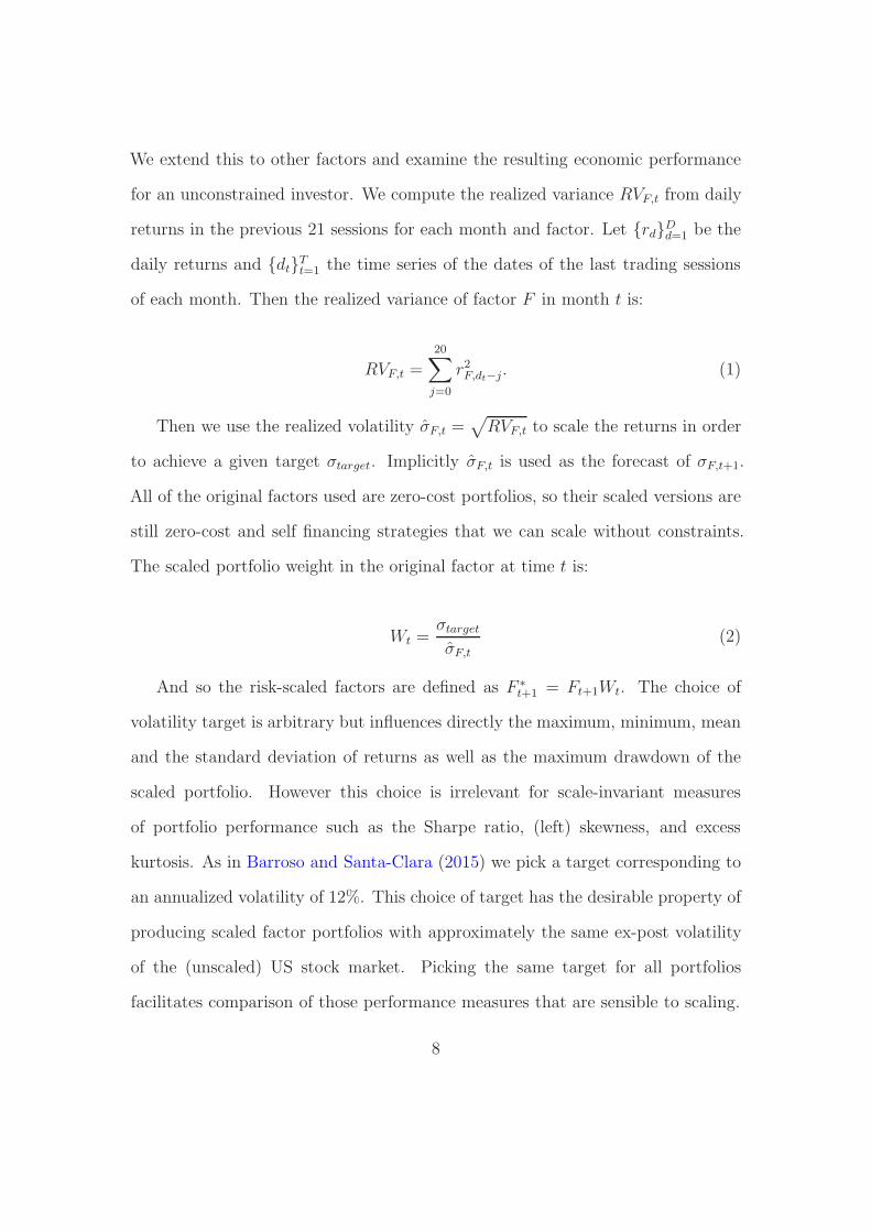
We extend this to other factors and examine the resulting economic performance
for an unconstrained investor. We compute the realized variance RVF,t from daily
returns in the previous 21 sessions for each month and factor. Let {rd}Dd=1
be the
daily returns and {dt}Tt=1 the time series of the dates of the last trading sessions
of each month. Then the realized variance of factor F in month t is:
RVF,t =
20∑
j=0
r2F,dt−j. (1)
Then we use the realized volatility σ̂F,t =√
RVF,t to scale the returns in order
to achieve a given target σtarget. Implicitly σ̂F,t is used as the forecast of σF,t+1.
All of the original factors used are zero-cost portfolios, so their scaled versions are
still zero-cost and self financing strategies that we can scale without constraints.
The scaled portfolio weight in the original factor at time t is:
Wt =σtarget
σ̂F,t
(2)
And so the risk-scaled factors are defined as F ∗
t+1 = Ft+1Wt. The choice of
volatility target is arbitrary but influences directly the maximum, minimum, mean
and the standard deviation of returns as well as the maximum drawdown of the
scaled portfolio. However this choice is irrelevant for scale-invariant measures
of portfolio performance such as the Sharpe ratio, (left) skewness, and excess
kurtosis. As in Barroso and Santa-Clara (2015) we pick a target corresponding to
an annualized volatility of 12%. This choice of target has the desirable property of
producing scaled factor portfolios with approximately the same ex-post volatility
of the (unscaled) US stock market. Picking the same target for all portfolios
facilitates comparison of those performance measures that are sensible to scaling.
8
Other volatility models could produce more accurate estimates of risk with
increased potential for risk-scaling. We refrain from that pursuit in this paper
and chose to focus instead on this somehow coarse measure of volatility. This also
serves as an implicit control mechanism when assessing the existence of robust
economic benefits in risk-scaling.3
[Insert table 3 near here]
Table 3 shows the performance of the scaled factors. Risk-scaling has economic
gains for investors following (almost) all factor strategies. For the market, the
risk-scaled factor has an information ratio of 0.20 with respect to the unscaled
factor. This gain confirms the result of Fleming et al. (2001) who document the
economic benefits of timing the volatility of the market. Their documented gains
from market timing using volatility contrast with the difficulty of similar strategies
trying to use predictability in returns (Goyal and Welch (2008)).
The benefits are not restricted to the market factor as 6 out of the 7 portfolios
show positive information ratios. The exception is the size premium for which the
scaled factor has a negative information ratio. Moskowitz (2003) show that the
size premium increases with volatility and recessions in a way consistent with a
risk-based explanation. Our results are consistent with theirs for the size factor.
By far the most impressive gains are found for the momentum and BAB factors.
Comparing with table 1 the Sharpe ratio of momentum increases from 0.67 to 1.08
(a 0.41 gain) and that of BAB increases from 0.91 to 1.28 (a 0.37 gain). The
information ratio of the scaled strategies with respect to their original versions
are very large for these two factors: 0.93 for MOM* and 0.94 for BAB*. These
3As a robustness test we also use the usual workhorse of volatility modelling, the GARCH(1,1).We present those results in table 6.
9
high information ratios reflect the fact that the risk-scaled portfolios are highly
correlated with the original factors but much more profitable. For the FF5 factors
the information ratio is on average 0.15, momentum and BAB have information
ratios about 6 times larger. Our results for momentum confirm the findings of
Barroso and Santa-Clara (2015). Moreira and Muir (2016) recently examine the
benefits of risk management in a set of factors that includes the FF5 but do not
consider BAB. Therefore, to the best of our knowledge, we are the first to document
that BAB shares this puzzling feature with momentum: the two strategies have
particularly expressive economic benefits from risk management, gains that set
them both apart from the FF5 factors.
[Insert table 4 near here]
Table 4 shows the risk-adjusted performance of BAB*. The strategy has a very
high CAPM-alpha of 21.10% per year. The risk model with the best fit for the strat-
egy is the C4 that explains 25% of its CAPM-alpha ((21.10%-15.83%)/21.10%).
This is a smaller proportion than the almost half explained in table 2. So risk-
managed BAB offers more diversification benefits than BAB for diversified in-
vestors exposed to other equity factors. The smallest annualized alpha is a very
high 15.83% (with the C4 model) and the adjusted r-squares of the regressions
are all smaller than in table 2. This confirms that BAB* is of value for diversified
investors and more so than BAB.
[Insert figure 1 near here]
Figure 1 shows the cumulative returns of momentum, betting-against-beta and
their respective risk-managed versions. As the strategies considered are zero-cost
10
portfolios their returns are excess returns. In order to have gross returns we add
to each strategy the gross return of an investment in the risk-free rate. So each
moment in time the portfolio puts all wealth in the risk-free rate and combines
this with a long-short portfolio. 4
In a pure CAPM world none of the strategies in figure 1 should have any
drift but empirically they have had an impressive economic performance. One
US dollar invested in momentum in July 1963 grows to 9, 990 by the end of the
sample. For the betting-against beta strategy the investment grows to a more
modest amount of 1, 675 dollars but with much less risk than the momentum
strategy. The scaled strategies have similar ex post standard deviation (17.37 for
MOM* versus 16.84 for BAB*) but very different end results: the investment in
risk-managed momentum grows to 87, 843 but in the beta anomaly to 364, 121.
For comparison a similar investment in the US stock market grows to 139 US
dollars by the end of the sample. This illustrates with an investment approach
the extent of the puzzle in the performance of these strategies, particularly the
benefits derived from managing their risk. A related debate is whether investors
could attain these performances in a realistic setting with transactions costs and
other frictions (see for example Lesmond et al. (2004) and Asness et al. (2014a)
for different interpretations of the evidence).
We do not address this debate directly but one possible interpretation of our
results is that the economic performance of these strategies, without frictions,
seems too puzzling to accept any explanation that does not incorporate them.
4For example, for momentum the original strategy puts a notional amount in the long leg ofWealtht and in the short leg of −Wealtht. For the risk-managed version the notional amountwould be WtWealtht and −WtWealtht in the long and short legs respectively. For BAB theamounts in the long and short leg are different in order to target a beta of zero but they areoffset by positions in the T-bills.
11
From an asset pricing perspective it is relevant to distinguish between correct
prices driven by risk loadings from mispricings that are hard to arbitrage. The
sizeable benefits of risk-management for BAB deepen the puzzle of the anomaly
and provide further indirect evidence of its relation to explanations relying on
arbitrage and frictions.
3.1. Robustness test: GARCH (1,1)
We assess the robustness of our results with respect to the horizon used to
compute the realized variance and using the GARCH(1,1) instead to estimate
variance.
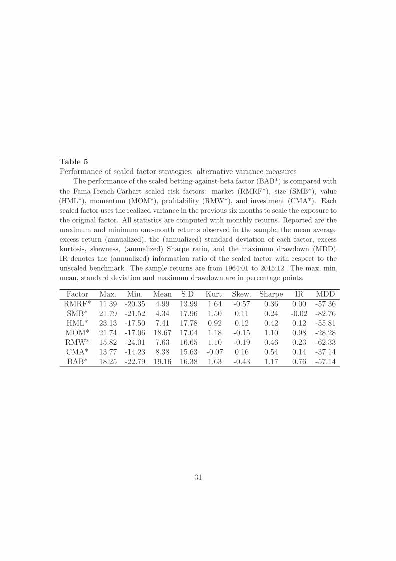
Table 5 shows the performance of scaled factors using 6 months to estimate
variance instead of just one. First we note that for this particular window the
result of the economic value of timing the volatility of the market is not robust.
[Insert table 5 near here]
The information ratio for risk-managed momentum is 0.98, so the benefits for
this strategy are robust to this alternative period to compute variance. For BAB,
with a Sharpe ratio of 1.17 and an information ratio of 0.76 with respect to the
original strategy, we conclude that the benefits of risk-management are robust to
using an alternative window.
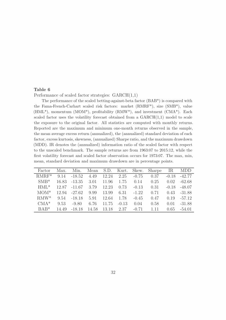
We also use GARCH(1,1) from monthly returns of each strategy to compute
risk-managed strategies. In order to assess the benefits of risk-management in
a realistic OOS environment we only use volatility estimates obtained from a
GARCH(1,1) model estimated in real time. We use the initial 120 months of
data to infer the parameters of the initial model and use them to make a forecast
12
for month 121. The following month we expand the sample with a new observation
and re-estimate the model. We keep re-iterating the procedure until the end of the
sample. Table 6 shows the economic performance of the risk-managed portfolios.
For comparison table 7 shows the performance of the original strategies for this
different sample period.
[Insert tables 6 and 7 near here]
In this setting the benefits of risk-management for the market are not robust
with a negative information ratio of -0.18. For momentum the benefits are robust
with a gain in Sharpe ratio from 0.57 to 0.71 and a substantial reduction in the
maximum drawdown from -80.36% to just -31.88%. For BAB the results are quite
robust. The information ratio of BAB* is 0.65, even higher than the 0.43 of MOM*.
So in this particular exercise the benefits of risk-management for BAB are stronger
than for MOM.
4. Risk and return of BAB
We examine the predictability of the risk of BAB and its relation with expected
returns.
First we examine the predictability of risk. Figure 2 shows the time series of
the (annualized) monthly realized variances computed from daily returns.
[Insert figure 2 near here]
The plot illustrates the typical patterns of volatility known from Bollerslev
(1987), Schwert (1989) and many others. Namely, volatility varies over time in a
13
persistent manner. The realized volatility of the strategy varies significantly from a
minimum of 1.75% in April 1965 to a maximum of 83% reached in May 2002. The
series is also highly non-normal with a kurtosis of 35.44 and a very high positive
skewness of 4.52 indicating that the sample contains extreme high risk outliers.
To examine the predictability of risk we run the regression:
1
ˆσi,t+1
= ρ0 + ρ11
σ̂i,t
+ εt+1. (3)
We focus on the inverse of realized volatility for two reasons. First, the risk-
managed strategy puts a weight on BAB proportional to this quantity so it is
the variable of direct interest to understand the source of the gains. Second, the
sample of the inverse of volatilities is much closer to normal. It has a kurtosis of
2.99 and a skewness of -0.11, this allows for a much better inference reducing the
large weight of outliers in the fit.
Table 8 shows the results of regression 3. Given the similar gains of risk manage-
ments for BAB and momentum we focus on these two strategies for the remainder
of the paper.
[Insert table 8 near here]
The table shows that both series have similar levels of predictability. The slope
coefficient is positive and it has a t-statistic of 23.88 for BAB and 25.31 for MOM.
This shows that safe months tend to follow safe months. Most of the variation in
the dependent variable is explained by its lagged value (R2 of 60.79% for BAB and
56.11% for MOM).
But in sample predictability can be misleading and so we also compute the out-
of-sample (OOS) R2 of the regression. For that purpose we use an initial window S
14
of 120 months ro run the first in-sample regression and use this to make a forecast
for month S + 1 that we compare with the ex-post realized value of the variable.
The following month we use an expanding window to estimate the regression and
re-iterate the procedure until the end of the sample. The OOS R2 for a factor i is
estimated as:
R2
i,OOS = 1−
T−1∑t=S
(ρ̂0,t + ρ̂1,t1̂/σi,t − ̂1/σi,t+1
T−1∑t=S
(1̂/σi,t − ̂1/σi,t+1)2, (4)
where 1̂/σi,t is the historical average up to time t and both α̂t and ρ̂t are
estimated with information available only up to time t. A positive OOS R2 shows
that on average the forecast from the regression outperforms that obtained from
the historical average.
We find the OOS R2 for BAB is not only positive but also very close to its
in-sample counterpart. This shows that the regression shows strong robustness out-
of-sample – a stark contrast with similar regressions for the equity premium that
typically achieve negative OOS R2’s (Goyal and Welch (2008)). The predictability
of the (inverse of) realized volatility for BAB is quite similar to the one documented
for momentum.
[Insert table 9 near here]
We next examine if this predictability in risk is related with expected returns.
For this purpose we regress the returns of each strategy on its lagged (inverse of)
realized volatility.
15
ri,t+1 = γ0 + γ1(1/σ̂i,t) + ηt+1. (5)
The existence of a risk-return trade-off should be captured by a statistically
significant negative γ1 meaning that months with less risk for the strategy also
predict smaller returns. The results in table 9 show there is no evidence of any
predictability of risk for the returns of BAB (or momentum). In fact the point
estimates for both strategies are positive, although not statistically significant.
[Insert figure 3 near here]
In figure 3 we further examine the relation between risk and return for the
strategies. For each strategy, we sort all months into quintiles according to realized
volatility. Then, for each quintile, we take the subset of months subsequent to
those in that quintile and compute the average return, standard deviation, and
Sharpe ratio over that subset. The results for momentum confirm the pattern in
Barroso and Santa-Clara (2015) that higher risk predicts both lower returns and
higher risk for the strategy, so the Sharpe ratio of the strategy is much higher
following quintiles 1 to 3 than in the two top quintiles. The results for BAB
show a similar pattern. In panel A the returns following a month in quintile 5
are lower (4.84%) on average than for other quintiles (11.53%). The relation is
not monotonous and the underperformance of BAB in terms of expected returns
is concentrated in months of particularly high risk. On the other hand, panel B
shows that subsequent risk rises monotonically with lagged risk. The annualized
volatility is 5.13% after a month in quintile 1 and it is 19.06% after a month in
quintile 5. As a result the Sharpe ratio is much smaller after months in the top
quintile (0.25) versus months after the lowest quintile (1.83). Both effects combine
16
such that BAB has a quite weak performance as a factor subsequent to months of
very high risk.
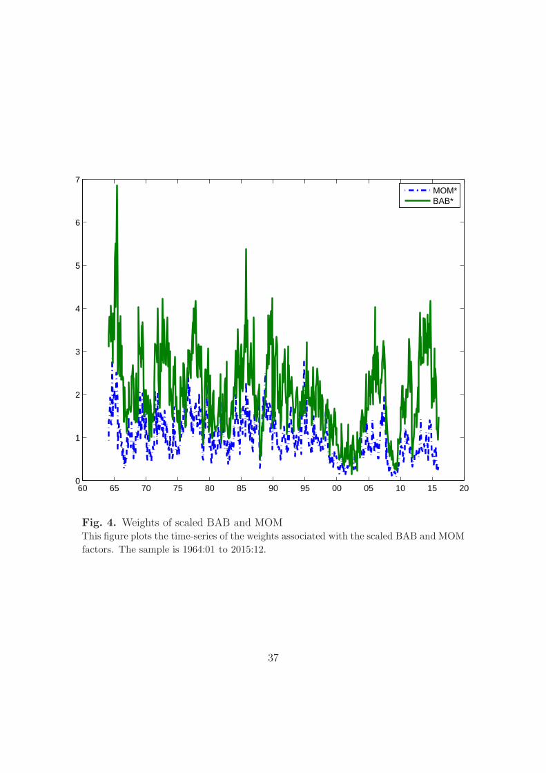
[Insert figure 4 near here]
Figure 4 shows the weights of BAB* and MOM*. On average BAB* has a
higher weight than MOM*. This happens because both strategies target the same
volatility but original BAB has a much lower standard deviation than MOM.5 As
the choice of target volatility is arbitrary this difference in the average weight is not
very informative. We note though that the two series have a strong and statistically
significant correlation of 0.63 (at the 1%) level. So an hypothetical unconstrained
arbitrageur following both strategies simultaneously would see speculative capital
being absorbed and freed-up from these two uses at the same time. This suggests
a possible limit to arbitrage for risk-management.
5. Anatomy of BAB risk
Grundy and Martin (2001) show that the beta of momentum with respect to
the market varies substantially over time. Cederburg and O’Doherty (2016) argue
that the conditional beta of BAB explains its premium. Motivated by this we
examine if time-varying systematic risk can account for the similar gains of risk
management for BAB and MOM and the performance of BAB in particular.
[Insert figure 5 near here]
5A version of BAB* re-scaled to have a similar average weight as MOM* would also show avery similar standard deviation in weights, so the apparent wilder swings of the weights in BABare only due to a level effect.
17
Figure 5 shows the plot of the time series of monthly betas of BAB and MOM
with respect to the market. The results for momentum confirm Grundy and Martin
(2001). The beta of MOM ranges between -2.86 and 2.57. We find that BAB also
has some time-varying market risk. In spite of being deliberately constructed to be
market neutral, its beta ranges between -1.57 and 0.30 and it shows some persis-
tence. Still the beta of BAB shows relatively little time-variation when compared
to momentum.
We use the CAPM to decompose the risk of BAB and MOM into a market and
a specific component:
RVF,t = β2
tRVRM,t + σ2
ε,t. (6)
The realized variances are estimated from daily returns in each month. 6 We
find that on average 37% of the risk of BAB is systematic, so the market neutral
strategy has a substantial market risk component. To assert the origin of the
gains, we examine the performance of a risk-managed strategy using each of the
risk components separately.
[Insert table 10 near here]
Table 10 shows the performance of risk-scaled BAB and momentum with total
risk, specific risk, and market risk respectively. The Sharpe ratio of BAB scaled
with specific risk is 1.21, close to the one using total risk (1.32). By contrast,
the strategy using the systematic risk has a very low Sharpe ratio of 0.18 and
6To ensure the decomposition holds exactly, we use in this section the variance formula. Thisde-means returns each month instead of just summing the squares of returns as in equation1. This does not change any of the results substantially and avoids the possibility of getting anegative specific risk.
18
a extreme value for standard deviation (3898.63), excess kurtosis (610.79), and
skewness (24.68). The results for momentum are similar to those of BAB. They
both show that the gains of risk-management come from using the informational
content in the specific component of risk.
We also examine the predictability of the inverse of each component of risk.
Table 11 shows the results of an auto-regression for each of those components
(which correspond to the weights in the strategies examined in table 10).
[Insert table 11 near here]
For BAB the specific part of risk is highly persistent with a slope coefficient
of 0.68 and a t-statistic of 20.30. The regression shows a good fit both in-sample
and OOS with R-squares of 46.13% and 47.46% respectively. The predictability
of the specific component is almost as high as that of total risk. For the sys-
tematic component there is no predictability. The slope coefficient is zero and
so is the R-squared. The results for momentum are similar and confirm those of
Barroso and Santa-Clara (2015). For both strategies the predictable part of risk
is the specific component.
6. Conclusion
Approximately half of the risk-adjusted returns of betting-against-beta with
respect to the market are explained by the Carhart (1997) or the Fama and French
(2015) factor models. While the remainder risk-adjusted performance is still a
puzzle in its own right, managing the risk of the strategy makes it much larger.
The risk-managed strategy has a high information ratio of 0.94, similar to that of
19
momentum. The scaled BAB has a higher alpha with respect to the market and
less of it (only 25%) is explained by equity risk factors. So managing the risk of
BAB creates and economic value orthogonal to those equity factors and even the
original BAB itself.
Risk is highly predictable for BAB, similar to that of momentum. There is also
no evidence of a risk-return trade-off for the strategy. If anything there seems to
be the opposite of a trade-off: BAB generally performs worse after months of high
risk in the strategy. This bad performance is concentrated in periods of extreme
risk for the strategy suggesting a regime switch in high volatility states.
Time-varying systematic risk has been proposed as an explanation of the pre-
mium of BAB (Cederburg and O’Doherty (2016)). We find evidence confirming
the existence of this time-varying systematic risk but also find that it conveys rela-
tively little information about the conditional performance of the strategy. Decom-
posing the risk of BAB into market and specific risk we find that the predictable
part is the specific one. Also, the performance of a strategy scaled by specific risk
only is very similar to one using total risk. So we conclude that specific risk is
causing the gains of risk management.
Generally, our results show that risk-managed BAB is a deeper puzzle than its
original version. The informational content of its own lagged volatility to condition
exposure to the strategy is very large, similar to momentum and much higher than
that found for the other equity factors examined.
The results are robust to using a different window to compute volatilities or a
GARCH(1,1) model to estimate it.
20
References
Antoniou, C., Doukas, J. A., and Subrahmanyam, A. (2015). Investor sentiment,
beta, and the cost of equity capital. Management Science, 62(2):347–367.
Asness, C. S., Frazzini, A., Israel, R., and Moskowitz, T. J. (2014a). Fact, fiction
and momentum investing. Journal of Portfolio Management, Fall.
Asness, C. S., Frazzini, A., and Pedersen, L. H. (2014b). Low-risk investing without
industry bets. Financial Analysts Journal, 70(4):24–41.
Baker, M., Bradley, B., and Taliaferro, R. (2014). The low-risk anomaly: A decom-
position into micro and macro effects. Financial Analysts Journal, 70(2):43–58.
Banz, R. W. (1981). The relationship between return and market value of common
stocks. Journal of financial economics, 9(1):3–18.
Barroso, P. and Santa-Clara, P. (2015). Momentum has its moments. Journal of
Financial Economics, 116(1):111–120.
Basu, S. (1983). The relationship between earnings’ yield, market value and return
for nyse common stocks: Further evidence. Journal of financial economics,
12(1):129–156.
Black, F., Jensen, M. C., and Scholes, M. S. (1972). The capital asset pricing
model: Some empirical tests. In Jensen, M., editor, Studies in the Theory of
Capital Markets. Praeger Publishers Inc.
21
Bollerslev, T. (1987). A conditionally heteroskedastic time series model for specu-
lative prices and rates of return. The review of economics and statistics, pages
542–547.
Bondt, W. F. and Thaler, R. (1985). Does the stock market overreact? The
Journal of finance, 40(3):793–805.
Carhart, M. M. (1997). On persistence in mutual fund performance. The Journal
of finance, 52(1):57–82.
Cederburg, S. and O’Doherty, M. S. (2016). Does it pay to bet against beta?
on the conditional performance of the beta anomaly. The Journal of finance,
71(2):737–774.
Cohen, R. B., Polk, C., and Vuolteenaho, T. (2005). Money illusion in the stock
market: The modigliani-cohn hypothesis. The Quarterly journal of economics,
120(2):639–668.
Damodaran, A. (2012). Investment valuation: Tools and techniques for determin-
ing the value of any asset, volume 666. John Wiley & Sons.
Daniel, K. D. and Moskowitz, T. J. (2016). Momentum crashes. Journal of
Financial Economics, 122(2):221–247.
Fama, E. F. and French, K. R. (1993). Common risk factors in the returns on
stocks and bonds. Journal of financial economics, 33(1):3–56.
Fama, E. F. and French, K. R. (2004). The capital asset pricing model: Theory
and evidence. The Journal of Economic Perspectives, 18(3):25–46.
22
Fama, E. F. and French, K. R. (2015). A five-factor asset pricing model. Journal
of Financial Economics, 116(1):1–22.
Fleming, J., Kirby, C., and Ostdiek, B. (2001). The economic value of volatility
timing. The Journal of Finance, 56(1):329–352.
Frazzini, A. and Pedersen, L. H. (2014). Betting against beta. Journal of Financial
Economics, 111(1):1–25.
Goyal, A. and Welch, I. (2008). A comprehensive look at the empirical performance
of equity premium prediction. Review of Financial Studies, 21(4):1455–1508.
Grundy, B. D. and Martin, J. S. M. (2001). Understanding the nature of the risks
and the source of the rewards to momentum investing. Review of Financial
studies, 14(1):29–78.
Hou, K., Xue, C., and Zhang, L. (2014). Digesting anomalies: An investment
approach. Review of Financial Studies.
Huang, S., Lou, D., and Polk, C. (2015). The booms and busts of beta arbitrage.
Available at SSRN 2666910.
Jegadeesh, N. (1990). Evidence of predictable behavior of security returns. The
Journal of Finance, 45(3):881–898.
Jegadeesh, N. and Titman, S. (1993). Returns to buying winners and selling losers:
Implications for stock market efficiency. The Journal of finance, 48(1):65–91.
Jegadeesh, N. and Titman, S. (1995). Short-horizon return reversals and the bid-
ask spread. Journal of Financial Intermediation, 4(2):116–132.
23
Lesmond, D. A., Schill, M. J., and Zhou, C. (2004). The illusory nature of mo-
mentum profits. Journal of financial economics, 71(2):349–380.
Levy, R. A. (1967). Relative strength as a criterion for investment selection. The
Journal of Finance, 22(4):595–610.
Lintner, J. (1965). The valuation of risk assets and the selection of risky invest-
ments in stock portfolios and capital budgets. The review of economics and
statistics, pages 13–37.
Mehra, R. and Prescott, E. C. (1985). The equity premium: A puzzle. Journal of
monetary Economics, 15(2):145–161.
Moreira, A. and Muir, T. (2016). Volatility managed portfolios. The journal of
finance, forthcomming.
Moskowitz, T. J. (2003). An analysis of covariance risk and pricing anomalies.
Review of Financial Studies, 16(2):417–457.
Novy-Marx, R. (2013). The other side of value: The gross profitability premium.
Journal of Financial Economics, 108(1):1–28.
Rosenberg, B., Reid, K., and Lanstein, R. (1985). Persuasive evidence of market
inefficiency. The Journal of Portfolio Management, 11(3):9–16.
Schwert, G. W. (1989). Why does stock market volatility change over time? The
journal of finance, 44(5):1115–1153.
Sharpe, W. F. (1964). Capital asset prices: A theory of market equilibrium under
conditions of risk. The journal of finance, 19(3):425–442.
24
Treynor, J. L. (1965). How to rate management of investment funds. Harvard
business review, 43(1):63–75.
25
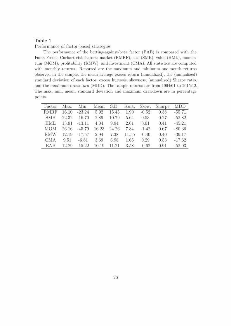
Table 1Performance of factor-based strategies
The performance of the betting-against-beta factor (BAB) is compared with the
Fama-French-Carhart risk factors: market (RMRF), size (SMB), value (HML), momen-
tum (MOM), profitability (RMW), and investment (CMA). All statistics are computed
with monthly returns. Reported are the maximum and minimum one-month returns
observed in the sample, the mean average excess return (annualized), the (annualized)
standard deviation of each factor, excess kurtosis, skewness, (annualized) Sharpe ratio,
and the maximum drawdown (MDD). The sample returns are from 1964:01 to 2015:12.
The max, min, mean, standard deviation and maximum drawdown are in percentage
Fig. 1. The cumulative returns of BAB, MOM and its risk-managed versionsusing the previous month realized volatility. The returns are from 1964:01 to2015:12 and include the return of the risk-free rate asset plus the excess return ofthe respective zero-cost portfolio.
30
Table 5Performance of scaled factor strategies: alternative variance measures
The performance of the scaled betting-against-beta factor (BAB*) is compared with
the Fama-French-Carhart scaled risk factors: market (RMRF*), size (SMB*), value
(HML*), momentum (MOM*), profitability (RMW*), and investment (CMA*). Each
scaled factor uses the realized variance in the previous six months to scale the exposure to
the original factor. All statistics are computed with monthly returns. Reported are the
maximum and minimum one-month returns observed in the sample, the mean average
excess return (annualized), the (annualized) standard deviation of each factor, excess
kurtosis, skewness, (annualized) Sharpe ratio, and the maximum drawdown (MDD).
IR denotes the (annualized) information ratio of the scaled factor with respect to the
unscaled benchmark. The sample returns are from 1964:01 to 2015:12. The max, min,
mean, standard deviation and maximum drawdown are in percentage points.