EUROGRAPHICS 2008 / G. Drettakis and R. Scopigno (Guest Editors) Volume 27 (2008), Number 2 Manifold-valued Thin-Plate Splines with Applications in Computer Graphics Florian Steinke 1 , Matthias Hein 2 , Jan Peters 1 , and Bernhard Schölkopf 1 1 Max Planck Institute for Biological Cybernetics, Tübingen, Germany 2 Saarland University, Saarbrücken, Germany Abstract We present a generalization of thin-plate splines for interpolation and approximation of manifold-valued data, and demonstrate its usefulness in computer graphics with several applications from different fields. The cornerstone of our theoretical framework is an energy functional for mappings between two Riemannian manifolds which is independent of parametrization and respects the geometry of both manifolds. If the manifolds are Euclidean, the energy functional reduces to the classical thin-plate spline energy. We show how the resulting optimization problems can be solved efficiently in many cases. Our example applications range from orientation interpolation and motion planning in animation over geometric modelling tasks to color interpolation. Categories and Subject Descriptors (according to ACM CCS): I.3.5 [Computer Graphics]: Computational Geometry and Object Modelling, Splines 1. Introduction Thin-plate splines (TPS) are a standard tool in computer graphics and also in many other disciplines both for inter- polation and approximation. So far, most work has been fo- cused on Euclidean output data, for example in trajectory design with control points in R 3 or in implicit surface recon- struction. The current paper generalizes thin-plate splines to the case where the output space is a Riemannian manifold. In computer graphics data living on manifolds occur quite naturally. Some basic types are directions, angles, and ori- entations, as well as smooth surfaces of objects and colors. More generally any data in Euclidean space which under- lie smooth constraints can be seen as lying on a manifold. Therefore manifold-valued interpolation/approximation is of general interest in computer graphics. 1.1. Related Work Thin-plate splines are characterized as the minimizers of a differential energy, the squared Frobenius norm of the Hessian subject to data interpolation/approximation con- straints. Research in manifold-valued splines has up to now mainly focused on curves, in which case thin-plate splines are equivalent to well-known cubic splines. Cubic splines Ψ Figure 1: Manifold-valued thin-plate spline Ψ mapping a 2D region onto a 3D bunny model using five markers. have been generalized to manifold-valued data in [GK85, NHP89, BCGH92] by replacing the standard derivative with the intrinsic covariant derivative on the manifold. Recently, an approach using the second extrinsic derivative has been investigated in [HP04] and then generalized to a network of curves in [WPH07]. For a broad overview of existing tech- niques for interpolating curves on manifolds, with an eye on motion planning, see [NP07]. The energy of mappings between Riemannian manifolds has been first studied by Eells and Sampson [ES64]. They define an energy based on the first-order differential of the c 2008 The Author(s) Journal compilation c 2008 The Eurographics Association and Blackwell Publishing Ltd. Published by Blackwell Publishing, 9600 Garsington Road, Oxford OX4 2DQ, UK and 350 Main Street, Malden, MA 02148, USA.
Transcript
EUROGRAPHICS 2008 / G. Drettakis and R. Scopigno(Guest Editors)
Volume 27 (2008), Number 2
Manifold-valued Thin-Plate Splineswith Applications in Computer Graphics
Florian Steinke1, Matthias Hein2, Jan Peters1, and Bernhard Schölkopf1
1Max Planck Institute for Biological Cybernetics, Tübingen, Germany2Saarland University, Saarbrücken, Germany
AbstractWe present a generalization of thin-plate splines for interpolation and approximation of manifold-valued data, anddemonstrate its usefulness in computer graphics with several applications from different fields. The cornerstoneof our theoretical framework is an energy functional for mappings between two Riemannian manifolds whichis independent of parametrization and respects the geometry of both manifolds. If the manifolds are Euclidean,the energy functional reduces to the classical thin-plate spline energy. We show how the resulting optimizationproblems can be solved efficiently in many cases. Our example applications range from orientation interpolationand motion planning in animation over geometric modelling tasks to color interpolation.
Categories and Subject Descriptors (according to ACM CCS): I.3.5 [Computer Graphics]: Computational Geometryand Object Modelling, Splines
1. Introduction
Thin-plate splines (TPS) are a standard tool in computergraphics and also in many other disciplines both for inter-polation and approximation. So far, most work has been fo-cused on Euclidean output data, for example in trajectorydesign with control points in R3 or in implicit surface recon-struction. The current paper generalizes thin-plate splines tothe case where the output space is a Riemannian manifold.
In computer graphics data living on manifolds occur quitenaturally. Some basic types are directions, angles, and ori-entations, as well as smooth surfaces of objects and colors.More generally any data in Euclidean space which under-lie smooth constraints can be seen as lying on a manifold.Therefore manifold-valued interpolation/approximation isof general interest in computer graphics.
1.1. Related Work
Thin-plate splines are characterized as the minimizers ofa differential energy, the squared Frobenius norm of theHessian subject to data interpolation/approximation con-straints. Research in manifold-valued splines has up to nowmainly focused on curves, in which case thin-plate splinesare equivalent to well-known cubic splines. Cubic splines
Ψ
Figure 1: Manifold-valued thin-plate spline Ψ mapping a2D region onto a 3D bunny model using five markers.
have been generalized to manifold-valued data in [GK85,NHP89, BCGH92] by replacing the standard derivative withthe intrinsic covariant derivative on the manifold. Recently,an approach using the second extrinsic derivative has beeninvestigated in [HP04] and then generalized to a network ofcurves in [WPH07]. For a broad overview of existing tech-niques for interpolating curves on manifolds, with an eye onmotion planning, see [NP07].
The energy of mappings between Riemannian manifoldshas been first studied by Eells and Sampson [ES64]. Theydefine an energy based on the first-order differential of the
F. Steinke, M. Hein, J. Peters, & B. Schölkopf / Manifold-valued Thin-Plate Splines
mapping. The local extrema of this energy are the so calledharmonic maps. Since distortion-free (isometric) mappingsare harmonic, discrete harmonic mappings with Euclideanoutput are commonly used, e.g., in [ZRS05]. A method forinterpolation/approximation of manifold-valued data basedon the harmonic energy has been proposed in [MSO04].
1.2. Roadmap
The aim of this paper is to generalize thin-plate splines fromthe Euclidean to the manifold setting, or equivalently gen-eralize cubic splines on curved spaces to the case whereone has multivariate input. We will define a suitable energyfor multivariate mappings between two manifolds, whichreduces to the thin-plate spline energy if both manifoldsare Euclidean. The parametrization independent energy willonly use intrinsic geometric properties of the manifold. Wewill show that similar to the difference between cubic andlinear splines, our method leads to a smoother solution thanusing the harmonic energy which is based on the first orderderivative. Special attention will be given to the boundaryand appropriate boundary conditions. This will allow us tosmoothly extrapolate the mapping outside of the data range,without fixing the boundary a priori. Note that extrapolationis not possible in the formulation of cubic splines on curvedspaces in [GK85, NHP89, BCGH92, HP04] since start andend points of the curve need to be fixed.
Particular emphasis will be placed on the efficient imple-mentation of the corresponding optimization problem. Webelieve that the theoretical soundness, the relatively easy andefficient implementation, and a wide range of possible appli-cations provide the potential that the manifold-valued gener-alization of thin-plate splines will become a standard tool,just as their Euclidean equivalent.
After a sketch of the theoretical framework in Section 2we will describe in Section 3 the implementation of the op-timization problem in detail. We demonstrate the methodon several examples, namely interpolation of rotations (Sec-tion 4.1), learning of task-space tracking (Section 4.2), map-ping two dimensional regions onto smooth surfaces (Sec-tion 4.3), and color interpolation (Section 4.4).
2. Theoretical framework
We would like to define an energy functional for a mappingφ : M → N between two Riemannian manifolds M and N.Three objectives should hold for the energy functional.
1. independence of the parametrization of M and N,2. intrinsic formulation, that is it should only depend on the
geometry of M and N,3. penalization of the second order differential. In particular
for M⊆Rm and N ⊆Rn it should reduce to the thin-platespline energy,
SThinPlate(φ) =∫
M⊆Rm
m
∑α,β=1
p
∑µ=1
(∂
2φ
µ
∂xα∂xβ
)2dx.
The first objective means that the energy should not dependon the coordinate representation of the manifold, e.g., theenergy of curves on the sphere should be the same if we rep-resent the sphere in spherical or stereographic coordinates.This can be achieved by formulating the energy in the covari-ant language of differential geometry. The second require-ment is that the energy should only depend on the geome-try of M and N, that is only intrinsic properties of M andN should matter. In particular, if M and N are isometricallyembedded in Euclidean space like the sphere S2 in R3 orSO3 in R3×3, no properties of the ambient spaces should betaken into account, since the embedding is not unique. Thethird objective is motivated by the fact that an energy func-tional only penalizing the first order differential leads onlyto piecewise differentiable solutions as is shown below.
We call the resulting energy functional Eells energy afterJames Eells, who pioneered the study of harmonic maps be-tween Riemannian manifolds. The derivation requires someheavy machinery from differential geometry, for better read-ability we have moved it into the Appendix A-C. Here, wepresent a particular simple form of the energy functional inthe case where the input manifold M is Euclidean and theoutput manifold N is a submanifold in Euclidean space Rp.These conditions on input and output manifold hold in mostof our example applications covering many fields of com-puter graphics. Let i : N → Rp be the isometric embeddingof N into Rp, which is just the identity map if N is a subman-ifold of Rp. Then we denote by Ψ = iφ the composition ofthe map φ : M→ N with the inclusion map i.
Introducing standard Cartesian coordinates in M ⊂ Rm
and Rp, the Eells energy can be written as
SEells(Ψ) =∫
M⊆Rm
m
∑α,β=1
p
∑µ=1
[(∂
2Ψ
µ
∂xα∂xβ
)>]2
dx, (1)
where > denotes the projection onto the tangent space of N.It can be shown that this form of the energy is equivalent tothe intrinsic formulation defined on N, although we are ap-parently using extrinsic properties, i.e. properties related toRp. The crucial difference to standard multivariate splines isthe projection> onto the tangent space. This way, we penal-ize only intrinsic variations.
It is instructive to discuss the difference in the caseof curves. For the interpolation of curves on mani-folds an extrinsic energy has been proposed by Hoferand Pottmann [HP04]. Their extrinsic energy is given
by∫
M⊆R ∑pµ=1
(∂
2Ψ
µ
∂t2
)2dt whereas the Eells energy re-
duces to the cubic spline energy for curves on mani-
folds∫
M⊆R ∑pµ=1
[(∂
2Ψ
µ
∂t2
)>]2
dt, as proposed in [GK85,
NHP89]. One can decompose the acceleration ∂2Ψ
µ
∂t2 into itstangential and normal component. Thus, in the extrinsic en-ergy, apart from the desired tangential, intrinsic accelerationone penalizes also the normal, extrinsic acceleration. The set
F. Steinke, M. Hein, J. Peters, & B. Schölkopf / Manifold-valued Thin-Plate Splines
of minimizers of both energies can therefore differ substan-tially. Since geodesics have zero intrinsic acceleration theyare clearly minimizing the Eells energy. This is quite desir-able since geodesics correspond to the most “simple” curveson manifolds. However, geodesics will not necessarily min-imize the extrinsic energy of [HP04] due to the penalizationof the normal component of the acceleration of the curve.
The domains M that we consider usually possess a bound-ary. Thus, we have to specify the behavior at the boundaryvia boundary conditions. Using variational techniques wefind the extremal equation of the Eells energy, see Theorem1 in Appendix A. We deduce sufficient boundary conditions(BC), see Equation 12, which for the case M ⊆ Rm can bewritten in extrinsic notation, see Theorem 2, as
m
∑α=1
Nα
(∂
2Ψ
µ
∂xα∂xβ
)>= 0,
m
∑α,β=1
Nα ∂
∂xβ
(∂
2Ψ
µ
∂xβ∂xα
)>= 0,
(2)
where Nα is the normal vector field at the boundary of M.Consideration of these boundary conditions is novel even forcubic splines on curved spaces. They allow the smooth ex-trapolation of the solution.
3. Implementation
Given the data points (xi,yi) with xi ∈M and yi ∈N, we gen-erally compute approximating splines. Denoting the squaredgeodesic distance in N by d2(., .), we minimize the func-tional
SEells(Ψ)+Ck
∑i=1
d2(yi,Ψ(xi)) (3)
over all Ψ : M→Rp subject to the conditions Ψ(x) ∈ N andboundary conditions (2). For large C objective (3) enforcesinterpolation.
If N is Euclidean, it can be shown that the minimizer of(3) is a weighted sum of basis functions, piecewise cubicpolynomials for curves, or thin-plate basis functions in themultivariate setting [HL93]. However, addition is not welldefined for points on general manifolds, thus we cannot hopefor such a nice expansion if N is a general manifold. Instead,we resort to discretization of the input space M which is stillvery efficient due to sparsity of all involved matrices.
Below we describe the necessary discretization steps, tak-ing special care of boundaries of the domain M. We showhow to minimize the resulting optimization problem effi-ciently using a geometrically motivated constrained Newtonapproach.
3.1. Discrete Formulation of the Optimization Problem
In our model applications shown below, we use the spaces[0,1], [0,1]2, and S1 as input manifolds M. We cover thesewith a regular grid with spacing h, allowing us to use stan-dard symmetric finite difference approximations for first and
second order derivatives. At the boundaries of M we usea virtual point scheme: for each discretization point on theboundary we compute the boundary normal, for points incorners there may be several. We construct for any boundarypoint in M two new "virtual" points outside the domain ofM by translating each boundary point along the normal vec-tor by h and 2h. The virtual points are added to the interiordiscretization points, yielding the set Xd of all d discretiza-tion points. Domains with non-constant metric or non-trivialboundary could be dealt with using an interpolation schemebetween non-uniformly spaced discretization points in M, oremploying techniques from [BCOS01] who discretize PDEson general manifolds.
We represent Ψ : M → Rp by its function values at thediscretization points, i.e. as a vector Ψ ∈ Rd p. Discrete ex-pressions for the first and second derivatives in directionα, β are stored in sparse block diagonal d p× d p matri-ces Dα, Dα,β. Rows corresponding to virtual points are leftblank. The matrices Fint , Fbd filter out rows correspond-ing to interior points, or boundary points respectively. Fromthe k data points (xi,yi) we build a vector y ∈ Rkp, and ablock diagonal kp×d p interpolation matrix S such that SΨ
yields weighted k-nearest neighbor estimates of Ψ(xi). Thed p×d p matrix PΨ
t is the orthogonal projection of Rd p vec-tors onto the tangent spaces of the output manifold N at posi-tions encoded in Ψ. Lastly, Nα are diagonal matrices storingthe α components of the boundary normals at the discretiza-tion points on the boundary. In matrix notation problem (3)then reads
minΨ ∑α,β
ΨT DT
α,β
(PΨ
t)T FintPΨ
t Dα,βΨ+Cd2(SΨ,y)
s.t. ∑α
NαFbdPΨt Dα,βΨ = 0 ∀ β = 1, .., p (4)
∑α,β
NαFbdDβPΨt Dβ,αΨ = 0
Ψ(x) ∈ N ∀ x ∈ Xd .
To exemplify the notation we sketch it for map-pings Ψ : [0,1] → S2 ⊂ R3. Here, Xd = −2h,−h, ..,1 +2h where −2h,−h,1 + h,1 + 2h are the virtual points.We stack the different output components of Ψ aboveeach other, Ψ = (Ψ1(−2h),Ψ1(−h), ..,Ψ3(1 + 2h))T .D1,D11,Fbd ,Fint ,S,N1 are block-diagonal matrices withthree identical sub-blocks, one for each output dimension.It is Dsub
1,i j = δi, j+1− δi, j−1, except for the blank rows 1,d.Fsub
bd,i j = δi=1, j=3 + δi=2, j=d−2 since the left (right) bound-ary point has index 3 (d− 2) in Xd . Corresponding surfacenormals in M are stored as N1,sub = diag(−1,1). PΨ
t is as-sembled from individual projections PΨ(x)
t ∈ R3×3, x ∈ Xd .
3.2. Optimization
Optimization problem (4) closely resembles a linear con-strained quadratic problem, that could be solved in one New-ton step. However, the geodesic distance function d2(., .), the
and solve system (6) for x = Ψ. δΨ←Ψ−Ψ06: t∗ = argmint>0 Energy
(ProjectOnN(Ψ0 + tδΨ)
)7: Ψ← ProjectOnN(Ψ0 + t∗δΨ)8: until ‖Ψ−Ψ0‖∞ < threshold
constraint Ψ(x)∈N, and the dependence of PΨt on Ψ rule out
such a direct approach. Instead, as outlined in algorithm 1,we solve the problem iteratively, approximating (4) in eachstep with the closest linearly constrained quadratic problem.This numerical scheme turned out to be robust and efficient,typically converging in few iterations.
Given a current solution Ψ0, we replace the non-linearconstraint Ψ(x)∈N at each point with a geometrically moti-vated linear alternative: We constrain δΨ(x) = Ψ(x)−Ψ0(x)to lie in the tangent space of N at Ψ0(x). Furthermore, thenon-linear squared geodesic distance function d2(SΨ,y) isapproximated by a Euclidean distance term. We compute thegeodesic distance from SΨ to y, and place a virtual target yin the tangent plane of SΨ in direction of y at the computeddistance value. This way, the Euclidean term ‖SΨ− y‖2 hasthe same value and gradient as the replaced d2(SΨ,y). For-mally, y = SΨ0− 1
2∇d2(SΨ0,y).
In each iteration we then solve a constrained quadratic ob-jective of the form
minx
12
xT Ax−bT x s.t. Cx = d. (5)
Introducing Lagrange multipliers λ, the minimum isachieved by the solution of(
A CT
C 0
)(xλ
)=(
bd
). (6)
Since all involved matrices are extremely sparse, these prob-lems are amenable to efficient sparse solvers. For mediumto large problems we used the exact solver CHOLMOD[CDHR06], for very large problems preconditioned conju-gate gradient methods could be used. We add a small ridgeto increase numerical stability.
Having solved the quadratic problem, the vectors δΨ in-dicate a direction of descent. We perform a line search using
Goldstein’s rule. For each proposed step size we project thecorresponding Ψ back onto the manifold, and evaluate its en-ergy there. The optimization is terminated when the maximalchange of Ψ in one iteration is less than a small threshold.
As initial solution for the iterative scheme, we use the freesolution, projected onto the manifold N. I.e., we first com-pute the minimizer of (4) pretending the output space wasRp, in which case the problem is equivalent to the normalthin-plate spline solution. For complex output manifolds theprojection of the free Ψ onto N may introduce large distor-tions increasing the danger of local minima. Where neces-sary, we thus move Ψ slowly towards N in an iterative man-ner targeting a low Eells energy already for intermediate so-lutions. The squared distance of Ψ(x) to the closest point onN is added to objective (4) while the constraint Ψ(x) ∈ N isdropped. We solve for a new Ψ in each iteration with increas-ing weight on the distance term. To compute tangent spaceprojections for points Ψ(x) 6∈ N as required during this pro-cess, we use the iso-distance manifold to N through Ψ(x).
Note that it is mainly the constraint Ψ(x) ∈ N that cou-ples the different components of Ψ in (4). In the case whereN is Euclidean or where N is the direct sum of several Rie-mannian manifolds, all involved matrices are block diagonaland each component of Ψ can be computed separately. How-ever, the proposed algorithm is also quite efficient even forcoupled dimensions. Sparse solvers typically scale linearlywith the number of nonzero entries. As this number is pro-portional to the number of output dimensions in our case,the overall scaling of our algorithm is linear in the numberof output dimensions. It also scales sub-quadratically withthe number of discretization points, see Section 4.5. Sincethe number of discretization points grows exponentially withthe number of input dimensions, our approach is limited to asmall number of input dimensions. However, for many prob-lems in computer graphics, this is not a problem, since usu-ally the input dimension is low.
3.3. Operations on the output manifold
Our algorithm requires only three operations from the em-bedded output manifold N: (1) Projection of any point inthe embedding space onto the manifold. (2) Projection ontothe tangent space at any point of N. (3) Computation of thegeodesic distance and its derivative between any two pointsof the manifold N.
The implementation of these operations depends largelyon the way the manifold N is represented. For many mani-folds and their standard embeddings these steps are straight-forward. For N = S2 ⊂ R3, x,y ∈ R3, it is ProjectOnN(x) =x/‖x‖, the projection onto the tangent space Px
t = 1− xxT
xT x ,
the geodesic distance d2(x,y) = acos( xT y‖x‖‖y‖ )
2, and its
derivative∇xd2(x,y) = 2Pxt
x−y‖x−y‖
√d2(x,y).
Rotations respectively orientations as members of SO3
F. Steinke, M. Hein, J. Peters, & B. Schölkopf / Manifold-valued Thin-Plate Splines
(a) (b) (c) (d)
method: linear spline linear spline + Proj. Harmonic energy Eells energytarget space: angles R3 S2 S2
Figure 2: The interval [0,1] is mapped onto the unit sphere S2 in 3D. Green markers show the given data points yi ∈ S2, respective trainingtimes xi ∈ [0,1] are given as numbers close-by. Red markers indicate Ψ(xi) for the approximating spline Ψ : [0,1]→ S2. Yellow dots mark theΨ-images of equally spaced points in [0,1].
can be isometrically embedded in R9 as orthonormal 3× 3matrices. The induced distance is the absolute value of therotation angle. Different object specific metrics implement-ing a non-trivial inertia tensor are proposed in [HP04] andcan be dealt with similarly. The three operations are in thiscase: (1) The closest orthonormal matrix to any 3× 3 ma-trix can be found via the polar decomposition. (2) the tan-gent space of a point O of the Lie group SO3 is given byOJ |J ∈ Θ where Θ are the skew-symmetric matrices. (3)the geodesic distance between O1 and O2 is given as theFrobenius norm of the matrix logarithm log(O1OT
2 ).
We also experimented with surfaces in R3, which weregiven as densely sampled meshes. One approach would beto convert this discrete representation into a continuous dif-ferentiable one, e.g. by fitting an implicit surface descrip-tion [OBA∗03, MSO04]. However, we resorted to a muchsimpler scheme that worked well for densely sampled sur-faces. We extract surface normals for each vertex, and iden-tify the manifold close to a point x with the tangent plane ofthe closest vertex to x. Projection onto N and normal extrac-tion can then be done efficiently using fast nearest-neighborsearch. In order to determine geodesics, we first compute theshortest path on the given mesh using Dijkstra’s algorithm.With this as initialization, we then compute a harmonic map-ping (9) from [0,1] to the surface fixing the end points to thepoints for which the geodesic distances should be computed.This can be done with an implementation almost identical tothe one described above, just replacing second order deriva-tives with first order expressions. It is known that minimiz-ers of the harmonic energy are geodesics [ES64]. Note thatsmall geodesic distance in N implies also small Euclideandistance in Rp. In many of the examples below, we workedwith high weights C for the distance terms in (3), such thatalready after one iteration of the optimization algorithm thepoints were close with respect to the geodesic distance in N.From then on, we worked directly with the computationallycheaper Euclidean distance since the distances and gradientsare in this case almost identical.
4. Experiments
4.1. Interpolation on the Sphere and on SO3
We consider the approximation of a curve on the sphereS2 ⊆ R3 with 6 data points, see Figure 2. Before discussingmanifold-valued splines, we present some naive approaches,highlighting the difficulties of the problem. A first ideacould be to parameterize the surface of the sphere usingspherical coordinates, and to interpolate the coordinates ofthe data points using linear splines (For visualization pur-poses we use linear splines corresponding to first order dif-ferential energies here). This is computationally attractivesince the coordinates form a linear space, and the splinescan be computed using basis function expansions. How-ever, as shown in Figure 2(a), no path can go through theparametrization boundary −π,π, and the geometry is heav-ily distorted by the non-linear parametrization mapping fromS2 to (−π,π)× (0,π). Alternatively, shown in Figure 2(b),one could first compute a linear spline in R3 and then projectit onto the sphere. While the trajectory can now surround thesphere, the metric is still distorted. The yellow points areequally spaced in the input, however, close to the red arrowsthey are not equally spaced in the output.
Manifold adapted approaches are much better suited. InFigure 2(c), the harmonic energy (9) is used in the objec-tive (3), instead of the Eells energy. Note that that the yellowpoints are now equally spaced between any two data points,up to small distortions resulting from the 2D visualization.However, since the minimizers of the harmonic energy arepiecewise geodesic [MLH06], the curve is not differentiable.It also does not extend outside of the first/last marker. Us-ing the Eells energy both these problems are avoided, seeFigure 2(d). The curves are smooth and they extrapolate lin-early, or more precisely geodesically.
Similar effects are demonstrated in the video of this pa-per showing an interpolation from S1 to SO3 visualized asthe periodic rotation of a teapot. We use an embedding ofSO3 into R3×3 opposed to the quaternion based approachof [BCGH92] which is otherwise very similar.
F. Steinke, M. Hein, J. Peters, & B. Schölkopf / Manifold-valued Thin-Plate Splines
0 0.1 0.2 0.3 0.4 0.5 0.6 0.7 0.8 0.9 1−3.14
0
3.14
Mid
dle
An
gle
Time
0 0.1 0.2 0.3 0.4 0.5 0.6 0.7 0.8 0.9 1−3.14
0
3.14
Ou
ter A
ng
le
Time
(a) M
itsu
bis
hi P
A-1
0
(b) T
he
real
isat
ion
p
rob
lem
(c) S
om
e tr
ain
ing
p
osi
tio
ns
(d) l
earn
ed in
ner
an
gle
(e) T
raje
cto
ries
(f ) using standard controller (resolvced motion rate controller)
(g) using proposed controller
(h) Angle trajectories
q1l1
q2
q3
l2
l3
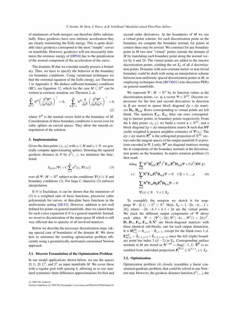
Figure 3: (a) Example system: Mitsubishi PA-10 with three planar DoFs where two have no joint limits (the others are locked). (b) Manypostures of a three link arm in two dimensions yield the same tip position. (c) Some training postures. (d) The inner most angle of the armgeneralized to the unit square in task space, R2. Angle−π corresponds to dark blue, π to dark red, training points are marked as black crosses.(e) The desired task space trajectory (red) is followed by both the resolved motion rate controller [SHV06] (blue) and our controller (green).The reachable space is yellow. (f,g) Postures during the trajectory. (h) Inner and outer angle plotted over time. The gray areas show the regionof the training values for the current x position (right hand side positive angles, left hand side negative ones).
4.2. Learning of Task-Space Tracking
Consider a skeleton based model in animation. As a runningexample we use a model of a robot arm, see Figure 3 (a).Most movement tasks are not defined through the model’sjoint angles q ∈ Sn
1 = S1×·· ·×S1 but rather by the motionof an end-effector x ∈ Rm, the fingertip. Thus, task-spaceplanning and control requires the inverse kinematic mappingof the task onto the joint space.
Most interesting models are redundant n > m, i.e. thereis a whole set of joint angles which all put the finger tip atthe same location. Some of these will look natural, otherswon’t. A controller that just focuses on keeping the end ef-fector on the desired trajectory may thus lead to rather unde-sirable postures. In practice it may be quite hard to specifyall (soft) constraints for a high-dimensional system explic-itly, and it may be much easier to specify a number of exam-ple postures. We therefore propose to generate joint-spacetrajectories that stay close to previously observed postures.
Typically, redundancy resolution is achieved by pullingthe robot towards a rest posture as implemented for exam-ple in the 3DSMax HI controller. Learning of postures hasbeen proposed by [GMHP04] who use Gaussian process re-gression. However, since some joints can rotate by 360 ourmanifold-valued thin-plate splines are much better suited forsuch a situation.
Formally, we assume that we are given a desired pathxd(t) ∈ Rm of the finger tip. At time t, we aim at determin-ing δq in the model’s joint angles q ∈ Sn
1 such that the newposture q+δq with tip position x(q+δq) is close to the de-sired position xd(t) and at the same time is similar to train-ing postures in this region of task space. For generalisinglocally preferred postures q1, ..,qk at positions x1, ..,xk toall reachable positions in task space, we use our generalizedthin-plate splines to learn a mapping qpred : Rm → Sn
1. Wethen choose δq such that it solves the optimization problem
min δq ‖x(q+δq)−x−δxd−κ[xd(t)−x]‖2 (7)
+λ1 ‖δq‖2 +λ2d2S3
1(q+δq,qpred(x)).
Firstly, this cost tries to keep the finger tip on the desiredtrajectory with a feedback term with gain κ. Secondly, weprefer small steps δq, and lastly try to minimise the distancebetween q + δq and suitably generalised training examplesqpred. The trade-off between the different objectives is con-trolled by the weighting coefficients λ1 and λ2. Taking thederivative of (7) with respect to δq and equating to zero wearrive at the following control law,
F. Steinke, M. Hein, J. Peters, & B. Schölkopf / Manifold-valued Thin-Plate Splines
(a) original in R2 (b) thin-plate to R3 + proj. (c) harmonic S2 (d) thin-plate to S2
Figure 4: The Lena image (a) is used to visualize a mapping from the unit square in R2 to the unit sphere S2 in R3. Green markers show thegiven data point pairs, red stars on S2 denote positions of the input markers in R2 mapped to the sphere by the approximating spline.
Figure 5: Thin-plate splines mapping a regular grid in R2 (yellow points) onto a face manifold in R3. Green and red markers as in Figure 4.
where J is the forward kinematic Jacobian J(q) = ∂x∂q (q).
The presented method is evaluated on the three link (n =3) arm model, see Figure 3 (a). For better visualization wechose a planar configuration (m = 2). Many postures q yieldthe same end effector location x, see Figure 3(b). Trainingpostures in Figure 3(c) are bent to the right for points x rightof the base, to the left otherwise. From 15 examples (blackcrosses in Figure 3(d)) we learn the function qpred(x); itsfirst component is color coded in Figure 3(d). Note the directtransition from −π to π would be impossible with normalthin-plate splines, since they are not aware of the fact that π
and −π actually encode the same angle. While the standardresolved motion rate controller [NCM∗05,SHV06] (λ2 = 0)results in intuitively quite unnatural poses (red boxes in Fig-ure 3(f,g)) despite a null-space term, ours stays close to themore natural training set. Also, when plotting the middle andouter angles — for which the training data imply a kind ofsoft constraints, see gray areas in Figure 3(h) — our con-troller consistently stays closer while full-filling the task tofollow xd(t) equally well as the default approach, see Fig-ure 3(e).
The above example is also visualized in the video of thispaper, where we compare against two alternatives. The re-solved motion rate controller [SHV06] (red) has no pre-ferred posture, the 3DSMAX HI inverse kinematics con-troller (blue) has a single one. In contrast, our approach(green) features location dependent preferred postures as
learned from a set of training examples. While it performssimilar to the 3DSMAX controller in the right half of thetask space, it smoothly adapts to the reverse curvature of thearm when entering the left half of task space.
4.3. Geometric Modelling
Here, we experiment with mappings from [0,1]2 ∈ R2 tosmooth surfaces in 3D. Such smooth mappings generatedfrom few data points are useful for many geometric mod-elling tasks such as surface parametrization, remeshing, ortexture mapping.
In parametrization, one typically computes mappingsfrom the surface to R2, see [SPR06] for an overview. How-ever, there are also many applications where the inversemapping is required. For this case, one could try to invertthe forward mapping, but this may be costly and the es-timated forward mapping need not even be invertible. Al-ternatively, one could directly estimate the inverse mappingfrom the R2 domain onto the manifold using our manifold-valued thin-plate splines. Similarly, one could use a regulargrid mapped onto the surface of an object, to reorganize themesh according to a 2D coordinate system. Such mappingsshould minimizes a reasonable measure of distortion. TheEells energy can be seen as such a measure of distortion. Itfollows from Proposition 2.21 in [EL83], see also [HSS08],that mappings have zero Eells energy if and only if theyare totally geodesic, which means that geodesics in M are
F. Steinke, M. Hein, J. Peters, & B. Schölkopf / Manifold-valued Thin-Plate Splines
mapped to geodesics in N. Every distortion free mapping istotally geodesic. The converse is generally not true but to-gether with enough training points one can find among allpossible totally geodesic mappings the one which is distor-tion free. Therefore for a given interpolation problem we cansee the Eells energy as a measure of the deviation from adistortion free mapping. This is in contrast to the harmonicenergy where totally geodesic maps are local extrema of theharmonic energy, but the value of the energy is zero if andonly if the map is constant, that is M is mapped to a sin-gle point in N. Therefore the Eells energy is a much bettermeasure of distortion than the harmonic energy.
In Figure 4 we compare different approaches for splinesfrom R2 to surfaces in R3 more closely. In Figure 4(b),we first compute thin-plate splines in R3, which yields aplane cutting through the given 4 markers in this case. Wethen project the plane onto the sphere. Observe the ex-treme fish-eye distortion resulting from projection. In Fig-ure 4(c), we show results for variational splines using theharmonic energy. This approach is commonly used in ge-ometric modelling, e.g., [ZRS05], although mostly target-ing linear spaces. However, the mapped image does not fillthe convex hull of the training points. This is why the har-monic energy is traditionally only used for input domainswithout boundary, or when the output boundary can be fixeda priori. [ZRS05] discusses a method to avoid this behav-ior, but one could alternatively use our proposed manifold-valued thin-plate splines, see Figure 4(d). Since the Eellsenergy does not try to minimize the distances between thepoints, but the variation of distances, it is much less prone tocontraction of the image. Furthermore, our generalized thin-plate splines extrapolate nicely out of the convex hull of themarker points.Similar effects are observed in Figure 5 showing a thin-platespline from R2 to a face manifold guided by 30 markers.These were placed on feature points of the face such as eyesand mouth, their input position in R2 was determined by pro-jecting the 3D points onto the surface of a vertical cylinderthrough the head. A more complex output manifold takenfrom the Stanford 3D Scanning Repository is used in Fig-ure 1.
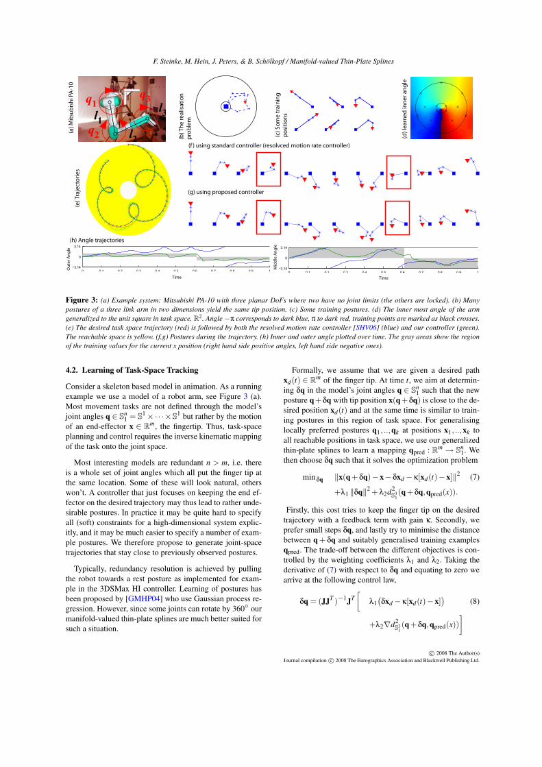
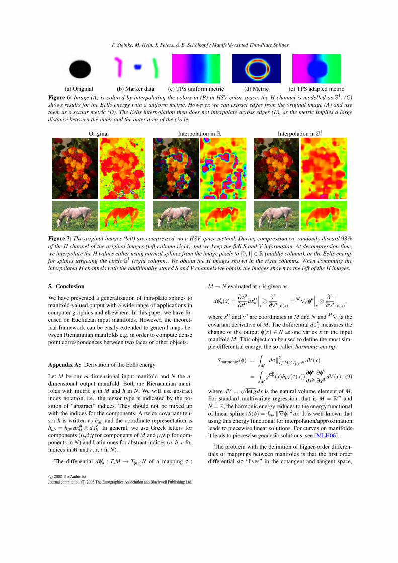
4.4. Color Interpolation
Another potential field of application for manifold-valuedsplines is color processing, since perceptually colors have acircular structure [She80]. This property is used in the HSVcolor space, where H, the hue value, is a circular variable.
For smoothing color values over an image, it makes senseto take into account the presence of edges. Edges can be in-cluded via a non-uniform metric in the input space. A onepixel distance could be termed large, if it crosses an edge,and small otherwise. This way our smoothing spline whichvaries slowly in units measured by the metric could expresssharp changes over edges, whereas it would vary slowly
within objects. A derivation and implementation hints aregiven in the Appendix D.
The effects are demonstrated in Figure 6, where we aim atcoloring a black and white image of a circle (a). We interpo-late given H color values (b) over the image, fixing the S andV channel values to 1. A uniform metric (c) misses to takeinto account the shape of the circle. We then compute thenorm of the (a)-image gradients in (d), a simple edge detec-tion scheme. Using these values as multiplier in the metric,we arrive at an interpolation that is much better suited to theimage structure (e).
The same technique is used for image compression in Fig-ure 7. The compression consists of the following steps: first,we transform the RGB image into HSV color space. Wesample randomly 500 pixels of H values, corresponding to2−3% of all values. We also store the S and V componentsfor the whole image. During decompression we interpolatethe H channel of the image using manifold-valued thin-platesplines. The mapping Ψ : R2→ S1 is learned using an edge-adapted metric as above, where the edges are extracted fromthe stored S and V channel. The HSV color image is finallytransformed back to normal RGB values. Some experimen-tal results are summarized below. RGB values range from 0to 1, the error is the RGB root mean squared error over thewhole image.
Horse FlowerImage size 135 x 200 133 x 100Error interpol. in R 0.029 0.144Error interpol. in S1 0.028 0.042
While the overall compression rate and quality is certainlynot state-of-the-art in well-developed image compression,the example may nevertheless show that manifold-valuedthin-plate splines are able to capture important regularitiesin natural datasets such as color images. It might be possibleto include such knowledge into a more sophisticated state-of-the-art compression scheme in the future.
4.5. Performance
Some run-times for our naive Matlab implementation ona dual core 2.2 GHz notebook are given below. For theLena problem, Figure 4, the run-time for one optimizationstep empirically scaled like O(d1.3) with the number of dis-cretization points d, an average of 3.5 optimization stepswere needed. Significant speed-ups and memory savingscould be achieved with an adaptive discretization scheme asis often used in finite element methods.
line Lena Lena Lena flower# discret. points 105 118 726 2.7k 14kTime [s] 0.14 0.21 2.1 13 122
The discretization error of Ψ for different spacings h be-tween discretization points reduced like O(h1.7) in the Lenaexample, when compared to results for a very fine discretiza-tion that was assumed to be identical with the continuoussolution.
F. Steinke, M. Hein, J. Peters, & B. Schölkopf / Manifold-valued Thin-Plate Splines
(a) Original (b) Marker data (c) TPS uniform metric (d) Metric (e) TPS adapted metricFigure 6: Image (A) is colored by interpolating the colors in (B) in HSV color space, the H channel is modelled as S1. (C)shows results for the Eells energy with a uniform metric. However, we can extract edges from the original image (A) and usethem as a scalar metric (D). The Eells interpolation then does not interpolate across edges (E), as the metric implies a largedistance between the inner and the outer area of the circle.
Original Interpolation in R Interpolation in S1
Figure 7: The original images (left) are compressed via a HSV space method. During compression we randomly discard 98%of the H channel of the original images (left column right), but we keep the full S and V information. At decompression time,we interpolate the H values either using normal splines from the image pixels to [0,1] ∈R (middle column), or the Eells energyfor splines targeting the circle S1 (right column). We obtain the H images shown in the right columns. When combining theinterpolated H channels with the additionally stored S and V channels we obtain the images shown to the left of the H images.
5. Conclusion
We have presented a generalization of thin-plate splines tomanifold-valued output with a wide range of applications incomputer graphics and elsewhere. In this paper we have fo-cused on Euclidean input manifolds. However, the theoret-ical framework can be easily extended to general maps be-tween Riemannian manifolds e.g. in order to compute densepoint correspondences between two faces or other objects.
Appendix A: Derivation of the Eells energy
Let M be our m-dimensional input manifold and N the n-dimensional output manifold. Both are Riemannian mani-folds with metric g in M and h in N. We will use abstractindex notation, i.e., the tensor type is indicated by the po-sition of “abstract” indices. They should not be mixed upwith the indices for the components. A twice covariant ten-sor h is written as hab and the coordinate representation ishab = hµν dxµ
a ⊗ dxνb. In general, we use Greek letters for
components (α,β,γ for components of M and µ,ν,ρ for com-ponents in N) and Latin ones for abstract indices (a, b, c forindices in M and r, s, t in N).
The differential dφra : TxM → Tφ(x)N of a mapping φ :
M→ N evaluated at x is given as
dφra(x) =
∂φµ
∂xαdxα
a
∣∣∣x⊗ ∂
r
∂yµ
∣∣∣φ(x)
= M∇aφµ∣∣∣x⊗ ∂
r
∂yµ
∣∣∣φ(x)
,
where xα and yµ are coordinates in M and N and M∇ is thecovariant derivative of M. The differential dφ
ra measures the
change of the output φ(x) ∈ N as one varies x in the inputmanifold M. This object can be used to define the most sim-ple differential energy, the so called harmonic energy,
Sharmonic(φ) =∫
M‖dφ‖2
T∗x M⊗Tφ(x)N dV (x)
=∫
Mgαβ(x)hµν(φ(x))
∂φµ
∂xα
∂φν
∂xβdV (x), (9)
where dV =√
detgdx is the natural volume element of M.For standard multivariate regression, that is M = Rm andN = R, the harmonic energy reduces to the energy functionalof linear splines S(φ) =
∫Rd ‖∇φ‖2 dx. It is well-known that
using this energy functional for interpolation/approximationleads to piecewise linear solutions. For curves on manifoldsit leads to piecewise geodesic solutions, see [MLH06].
The problem with the definition of higher-order differen-tials of mappings between manifolds is that the first orderdifferential dφ “lives” in the cotangent and tangent space,
F. Steinke, M. Hein, J. Peters, & B. Schölkopf / Manifold-valued Thin-Plate Splines
T∗x M and Tφ(x)N, of two different manifolds. Thus we can-not simply use the connection M∇ of M. The solution isto “pull-back” the connection N∇ of N for the covariantderivatives of elements in Tφ(x)N. The pull-back connection∇′ : TxM⊗Tφ(x)N→ Tφ(x)N is defined as
∇′ ∂
∂xα
∂r
∂yµ :=N ∇φ∗ ∂
∂xα
∂r
∂yµ =∂φ
ν
∂xα
NΓ
ρ
νµ∂
µ
∂yρ,
where NΓ
ω
νµ are the Christoffel-symbols of N.
With this definition, we have a notion of the derivative ofa vector field on N with respect to a variation in M, where Mand N are connected via φ. The covariant derivatives of thedifferential dφ
ra of φ : M→ N can thus be defined as
∇′bdφra := M∇b
M∇aφµ⊗ ∂
r
∂yµ + M∇aφµ⊗∇′b
∂r
∂yµ
=[
∂2φ
µ
∂xβ∂xα− ∂φ
µ
∂xγ
MΓ
γ
βα +∂φ
ρ
∂xα
∂φν
∂xβ
NΓ
µνρ
](10)
dxβ
b⊗dxαa ⊗
∂r
∂yµ .
Up to here the presented notions can be found in [EL83].
Equivalent to the the thin-plate spline case, we now usethe inner product in T∗x M⊗T∗x M⊗Tφ(x)N, yielding the Eellsenergy,
SEells(φ) =∫
M
∥∥∇′bdφra∥∥2
T∗x M⊗T∗x M⊗Tφ(x)NdV (x)
=∫
Mgacgb f hrs∇′bdφ
ra∇′ddφ
scdV (x). (11)
Appendix B: Variation of the Eells energy
Variation of the Eells energy provides us with necessary con-ditions for a minimizer and most importantly with boundaryconditions for M.
Theorem 1 Let φ(t,x) : (−ε,ε)×M→ N be a variation ofthe mapping φ = φ(0,x) and W r = ∂
∂t φrt∣∣t=0 the variational
vector field at t = 0. The variation of the Eells energy is givenas,
ddt
SEells(φt)∣∣∣t=0
=2∫
Mgab gcd hrs W r
[∇′c∇′a∇′bdφ
sd +RN
uvws dφ
wa dφ
uc ∇′bdφ
vd
]dV
+2∫
∂Mhrs gab Nd
[∇′aW r∇′ddφ
sb−W r ∇′a∇′bdφ
sd
]dV
where dV is the volume element of the boundary ∂M andRN
serb is the curvature tensor of N.
A necessary condition for a minimizer of the Eells en-ergy is d
dt SEells(φt)∣∣∣t=0
= 0 for all vector fields W . A set of
boundary conditions which achieves that the boundary termsvanish are
Na∇′adφrb = 0, Ncgab∇′a∇′bdφ
rc = 0. (12)
The proof is basically build on the two following Lemmas(proofs can be found in [HSS08]). The first one is a general-ization of the Green’s theorem for the pull-back connectionand the second one computes the commutator of the deriva-tive with respect to the variation and the pull-back connec-tion.
Lemma 1 Let R ∈ ⊗p+1T∗M⊗φ−1T N and S ∈ ⊗pT∗M⊗
φ−1T N, where φ
−1T N is the bundle of Tφ(x), x ∈ M. Thenwith∇′ being the pull-back connection,∫
M
⟨R,∇′S
⟩=
∫∂M〈R,N⊗S〉−
∫M
⟨traceg∇′R,S
⟩,
where N is the covector associated to the normal vector ofM and the trace is taken with respect to the first two indices.
Lemma 2 Let φ(t,x) : (−ε,ε)×M→ N be a variation of themapping φ = φ(0,x). Then
∂
∂t∇′adφ
rb =∇′a∇′b
∂φr
∂t+RN
suvr dφ
sa
dφu
dtdφ
vb. (13)
Proof We use the commutator from lemma 2 and obtain,
ddt
SEells(φt) = 2∫
Mgab gcd hrs
(∂
∂t∇′a(dφt)r
c
)∇′b(dφt)s
ddV
=2∫
Mgab gcd hrs∇′a∇′c
∂φr
∂t∇′b(dφt)s
ddV
+2∫
Mgab gcd hrs RN
uvwr (dφt)u
a∂φ
vt
∂t(dφt)w
c ∇′b(dφt)sd dV
One has ∇′b(dφt)sd
∣∣∣t=0
= ∇′bdφsd . We apply two times the
Green’s theorem of Lemma 1 and obtainddt
SEells(φt)∣∣∣t=0
= 2∫
Mgab gcd hrs∇′a∇′cW r ∇′bdφ
sd dV
+2∫
Mgab gcd hrs RN
uvwr dφ
ua W v dφ
wc ∇′bdφ
sd dV
=2∫
∂MNb gcd hrs∇′cW r ∇′bdφ
sd dV
−2∫
∂Mgab Nd hrs W r ∇′a∇′bdφ
sd dV
+2∫
Mgab gcd hrs W r ∇′c∇′a∇′bdφ
sd dV
+2∫
Mgab gcd hrs RN
uvwr dφ
ua W v dφ
wc ∇′bdφ
sd dV
=2∫
Mgab gcd hrs W r
[∇′c∇′a∇′bdφ
sd +RN
uvws dφ
wa dφ
uc ∇′bdφ
vd
]dV
+2∫
∂Mhrs gab Nd
[∇′aW r∇′ddφ
sb−W r ∇′a∇′bdφ
sd
]dV ,
where we have used in the last step Ruvws = Rwsuv.
Appendix C: From intrinsic to extrinsic representation
The expression of the Eells energy in coordinates is quitecomplicated as one can see from the explicit form of∇′bdφ
ra
in Eq. (10). However, the expression dramatically simplifyif N is an isometrically embedded submanifold of Rp and Mis a subset of Euclidean space Rm. We have to stress that the
F. Steinke, M. Hein, J. Peters, & B. Schölkopf / Manifold-valued Thin-Plate Splines
following reformulation of the energy is completely equiva-lent to the one in Eq. (11).
Let i : N → Rp be the isometric embedding and denoteby Ψ : M→ Rp the composition Ψ = i φ. Let zµ be stan-dard Cartesian coordinates in Rp. Then the differential of Ψ
is given as dΨra = ∂Ψ
µ
∂xα dxαa ⊗ ∂
r
∂zµ . As above we can also de-fine an pull-back connection ∇ : TxM⊗Tψ(x)Rp→ Tψ(x)Rp
for the mapping Ψ, ∇ ∂
∂xα
∂r
∂zµ := Rp∇
Ψ∗ ∂
∂xα
∂r
∂zµ = 0, which
is trivial due to the flatness of the connection of Rp. Be-cause of this property the expressions for the correspondingcovariant derivatives expression will simplify significantly.The following theorem shows how intrinsic expressions in φ
can be expressed in terms of the extrinsic ones in Ψ.
Theorem 2 The following equivalences between intrinsicand extrinsic objects hold,
dφra =dΨ
ra, ∇′bdφ
ra =
(∇bdΨ
ra)>
,
∇′c∇′bdφra =∇c
(∇bdΨ
ra)>−dΨ
sc
NΠ
rsu(∇bdΨ
ua)>
,
where > denotes the projection onto the tangent spaceTΨ(x)N and N
Πrsu is the second fundamental form of N. If
M is a domain in Rm we derive for the Eells energy (11) theexpression given in Eq. (1), for the corresponding boundaryconditions (12) the form (2).
The proof can be found in [HSS08]. Note that if M is a do-main in Rm one has
∇bdΨra =
∂2Ψ
µ
∂xα∂xβdxα
a ⊗dxβ
b⊗∂
r
∂yµ .
Appendix D: Non-uniform Metric in M
Consider the metric gi j(x) = Ω(x)δi j on M. For non-constantΩ, the Christoffel symbols M
Γκ
βα in the coordinate expres-sion of∇′bdΨ
rc in Eq. (10) do not vanish. We compute
∇′bdΨrc =
[∂
2Ψ
µ
∂xβ∂xα−
∂βΩ
2Ω
∂Ψµ
∂xα− ∂αΩ
2Ω
∂Ψµ
∂xβ
+∑γ
∂γΩ
2Ω
∂Ψµ
∂xγ
]dxβ
b⊗dxαc ⊗
∂r
∂yµ .
This is a linear expression in Ψ. For implementation wejust have to change the second derivative matrices Dα,β de-scribed in Section 3, by adding first order terms in form ofweighted combinations of Dα matrices.
References
[BCGH92] BARR A. H., CURRIN B., GABRIEL S., HUGHES
J. F.: Smooth interpolation of orientations with angular velocityconstraints using quaternions. Computer Graphics 26, 2 (1992),313–320.
[BCOS01] BERTALMIO M., CHENG L., OSHER S., SAPIRO G.:Variational problems and partial differential equations on implicitsurfaces. J. of Comp. Phys. 174, 2 (2001), 759–780.
[CDHR06] CHEN Y., DAVIS T., HAGER W., RAJAMANICKAM
S.: Algorithm 8xx: CHOLMOD, supernodal sparse Choleskyfactorization and update/downdate. ACM Trans. Math. Softw.,submitted in (2006).
[ES64] EELLS J., SAMPSON J. H.: Harmonic mappings of Rie-mannian manifolds. Amer. J. Math. 86, 1 (1964), 109–160.
[GK85] GABRIEL S., KAJIYA K.: Spline interpolation in curvedspace. In SIGGRAPH’85 Course Notes on State of the Art ImageSynthesis (1985), vol. 6, ACM Press, pp. 1–14.
[GMHP04] GROCHOW K., MARTIN S., HERTZMANN A.,POPOVIC Z.: Style-based inverse kinematics. ACM Transactionson Graphics 23, 3 (2004), 522–531.
[HL93] HOSCHEK J., LASSER D.: Fundamentals of ComputerAided Geometric Design. A. K. Peters, 1993.
[HP04] HOFER M., POTTMANN H.: Energy-minimizing splinesin manifolds. ACM Transactions on Graphics 23 (2004), 284–293.
[HSS08] HEIN M., STEINKE F., SCHÖLKOPF B.: Energyfunctionals for manifold-valued mappings and their proper-ties. Tech. Rep. 167, Max Planck Institute for Biolog-ical Cybernetics, Tübingen, Germany, 2008. available athttp://www.kyb.tuebingen.mpg.de/techreports.html.
[MLH06] MACHADO L., LEITE F. S., HÜPER K.: Riemannianmeans as solutions of variational problems. LMS J. Comput.Math. 9 (2006), 86–103.
[NCM∗05] NAKANISHI J., CORY R., MISTRY M., PETERS J.,SCHAAL S.: Comparative experiments on task space control withredundancy resolution. In Proc. IEEE/RSJ IROS (2005).
[NHP89] NOAKES L., HEINZINGER G., PADEN B.: CubicSplines on Curved Spaces. IMA Journal of Mathematical Controland Information 6 (1989), 465–473.
[NP07] NOAKES L., POPIEL T.: Geometry for robot path plan-ning. Robotica (2007), 1–11.
[OBA∗03] OHTAKE Y., BELYAEV A., ALEXA M., TURK G.,SEIDEL H.-P.: Multi-level partition of unity implicits. ACMTransactions on Graphics 22 (2003), 463–470.
[SHV06] SPONG M. W., HUTCHINSON S., VIDYASAGAR M.:Robot Modeling and Control. Wiley, 2006.
[SPR06] SHEFFER A., PRAUN E., ROSE K.: Mesh Parameteri-zation Methods and Their Applications. Foundations and Trendsin Computer Graphics and Vision 2, 2 (2006), 105–171.
[ZRS05] ZAYER R., RÖSSL C., SEIDEL H.: Setting the boundaryfree: A composite approach to surface parameterization. Sympo-sium on Geometry Processing (2005), 91–100.