71
Manipulator Dynamics Amirkabir University of Technology Computer Engineering & Information Technology Department
| Date post: | 21-Dec-2015 |
| Category: |
Documents |
| View: | 231 times |
| Download: | 6 times |

Manipulator Dynamics
Amirkabir University of TechnologyComputer Engineering & Information Technology Department

Introduction
Robot arm dynamics deals with the mathematical formulations of the equations of robot arm motion.They are useful as: An insight into the structure of the robot
system. A basis for model based control systems. A basis for computer simulations.
Equations of Motion
The way in which the motion of the manipulator arises from torques applied by the actuators, or from external forces applied to the manipulator.

Forward and Inverse Dynamics
,,,
,
Given a trajectory point, and find the required vectors of joint torques,
Given a torque vector, calculate the resulting motion of the manipulator, and
.
.,,
: problem of controlling the manipulator
: problem of simulating the manipulator

Two Approaches
Energy based: Lagrange-Euler.Simple and symmetric.
Momentum/force approach:Newton-Euler.
Efficient, derivation is simple but messy, involves vector cross product. Allow real time control.

Newton-Euler Algorithm
Newton-Euler method is described briefly below. The goal is to provide a big picture understanding of these methods without getting lost in the details.

Newton-Euler Algorithm
Newton-Euler formulations makes two passes over the links of manipulator
Forces, moments
Velocities, Accelerations
Gravity

Newton-Euler Algorithm
Forward computation First compute the angular velocity, angular
acceleration, linear velocity, linear acceleration of each link in terms of its preceding link.
These values can be computed in recursive manner, starting from the first moving link and ending at the end-effector link.
The initial conditions for the base link will make the initial velocity and acceleration values to zero.

Newton-Euler Algorithm
Backward computation Once the velocities and accelerations of the
links are found, the joint forces can be computed one link at a time starting from the end-effector link and ending at the base link.
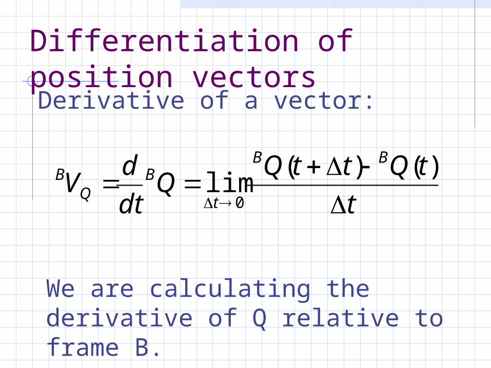
Differentiation of position vectors
t
tQttQQ
dt
dV
BB
t
BQ
B
)()(lim
0
We are calculating the derivative of Q relative to frame B.
Derivative of a vector:

Differentiation of position vectors
Qdt
dV B
A
QBA
A velocity vector may be described in terms of any frame:
.QBA
BQBA
VRV
We may write it:
VV CORG
U
C
Special case: Velocity of the origin of a frame relative to some understood universe reference frame
Speed vector is a free vector

Example 5.1
A fixed universal frame
30 mph
100 mph
.ˆ70)(
.ˆ100)ˆ100()(
.ˆ30
1
1
XRRVRRVRV
XRXRRvvV
XvVPdt
d
UT
UCCORG
TUT
CUCORG
TCTCORG
TC
UC
CUT
CUT
CTORG
UC
CCORGU
CORGU
U
Both vehicles are heeding in X direction of U

Angular velocity vector:
Linear velocity attribute of a point
Angular velocity attribute of a body
Since we always attach a frame to a body we can consider angular velocity as describing rational motion of a frame.

Angular velocity vector:describes the rotation of frame {B} relative to {A}
BA
BAMagnitude of
indicates speed of rotation
BA
CU
C
In the case which there is an understood reference frame:
direction of indicates instantaneous axis of rotation

Linear velocity of a rigid body
.QBA
BBORGA
QA VRVV
We wish to describe motion of {B} relative to frame {A}
RABIf rotation is not changing with time:

Rotational velocity of a rigid body
Two frames with coincident origins
The orientation of B with respect to A is changing in time.
Lets consider that vector Q is constant as viewed from B.
BA
QB{A}{B}
0QBV

Is perpendicular to and
Rotational velocity of a rigid body
QV
tQ
AB
AQ
A
BAAQ
)|)(|sin|(|||
BA
Magnitude of differential change is:
QA|| Q
Vector cross product

Rotational velocity of a rigid body
.QRVRV BABB
AQ
BABQ
A
In general case: QVV AB
AQ
BAQ
A )(

.QRVRVV BABB
AQ
BABBORG
AQ
A
Simultaneous linear and rotational velocity
We skip 5.4!

Motion of the Links of a Robot
At any instant, each link of a robot in motion has some linear andangular velocity.
Written in frame i

Velocity of a Link
Remember that linear velocity is associated with a point and angular velocity is associated with a body. Thus:
The velocity of a link means the linear velocity of the origin of the link frame and the rotational velocity of the link

Velocity Propagation From Link to Link
We can compute the velocities of each link in order starting from the base.
The velocity of link i+1 will be that of link i, plus whatever new velocity component added by joint i+1.
Rotational Velocity
Rotational velocities may be added when both w vectors are written with respect to the same frame.
Therefore the angular velocity of link i+1 is the same as that of link i plus a new component caused by rotational velocity at joint i+1.

Velocity Vectors of Neighboring Links
.ˆ1
1111
ii
ii
iii
ii ZR

By premultiplying both sides of previous equation to:
.ˆ
.ˆ
11
11
11
11
1111
11
ii
iiii
iii
ii
ii
iiii
iiii
iii
ZR
ZRRRR
Velocity Propagation From Link to Link
1
1
1
1
1 0
0
i
i
i
i
i Z
Note that:
Rii1

Linear Velocity
The linear velocity of the origin of frame {i+1} is the same as that of the origin of frame {i} plus a new component caused by rotational velocity of link i.

).(
).(
11
11
11
11
ii
ii
iii
iii
ii
ii
iii
iiii
i
PvRv
PvRvR
Linear Velocity
.QRVRVV BABB
AQ
BABBORG
AQ
A Simultaneous linear and rotational velocity:
.11 ii
ii
ii
ii Pvv
By premultiplying both sides of previous equation to: Ri
i1

.ˆ)(
,
11
111
11
11
1
ii
iii
ii
iii
iii
iii
iii
ZdPvRv
R
For the case that joint i+1 is prismatic:
Prismatic Joints Link

Velocity Propagation From Link to Link
Applying those previous equations successfully from link to link, we can compute the rotational and linear velocities of the last link.

Example 5.3
A 2-link manipulator with rotational joints
Calculate the velocity of the tip of the arm as a function of joint rates?

Example 5.3Frame assignments for the two link manipulator

.
1000
0100
0010
001
,
1000
0100
00
0
,
1000
0100
00
00 2
23
22
122
12
11
11
01
l
Tcs
lsc
Tcs
sc
T
Example 5.3
We compute link transformations:

.0
0
)(,
,
00
0
100
0
0
,0
0
,
0
0
0
,0
0
2
1
2221
21212121
121
33
22
33
121
121
1122
22
22
21
22
11
1
11
llcl
sllcl
sl
v
cl
sl
lcs
sc
v
v
Example 5.3
Link to link transformation

.
0
)(
)(
.
100
0
0
2
1
12212211
1221221121122111
21122111
330
330
1212
121223
12
01
03
clclcl
slslslclcl
slsl
vRv
cs
sc
RRRR
Example 5.3
Velocities with respect to non moving base

Derivative of a Vector Function
If we have a vector function r which represents a particle’s position as a function of time t:
dt
dr
dt
dr
dt
dr
dt
d
rrr
zyx
zyx
r
r

Vector Derivatives
We’ve seen how to take a derivative of a vector vs. A scalarWhat about the derivative of a vector vs. A vector?

Acceleration of a Rigid Body
Linear and angular accelerations:
.)()(
lim
,)()(
lim
0
0
t
ttt
dt
d
t
tVttVV
dt
dV
BA
BA
tB
AB
A
QB
QB
tQ
BQ
B

Linear Acceleration
).(2
)(
)()(
.)(
.
QRQRVRVR
QRVRQRVRVR
QRdt
dQRVR
dt
dV
QRVRQRdt
d
QRVRV
BABB
AB
ABABB
AQ
BABB
AQ
BAB
BABB
AQ
BABB
ABABB
AQ
BABB
AQ
BAB
BABB
ABABB
AQ
BABQ
A
BABB
AQ
BAB
BAB
BABB
AQ
BABQ
A
: origins are coincident.
: re-write it as.
: by differentiating.

.)(
.0
).(
2
QRQRVV
QVV
QR
QRVRVRVV
BABB
ABABB
AB
ABORG
AQ
A
BQ
BQ
B
BABB
AB
A
BABB
AQ
BABB
AQ
BABBORG
AQ
A
the case in which the origins are not coincident
: when is constant
: the linear acceleration of the links of a manipulator with rotational joints.
Linear Acceleration

Angular Acceleration
: the angular acceleration of the links of a manipulator.
B is rotation relative to A and C is rotating relative to B
.
.
.
CBA
BBA
CBA
BBA
CBA
BBA
CA
CBA
BBA
CA
RR
Rdt
d
R

InertiaIf a force acts of a body, the body will accelerate. The ratio of the applied force to the resulting acceleration is the inertia (or mass) of the body.If a torque acts on a body that can rotate freely about some axis, the body will undergo an angular acceleration. The ratio of the applied torque to the resulting angular acceleration is the rotational inertia of the body. It depends not only on the mass of the body, but also on how that mass is distributed with respect to the axis.

Mass Distribution
Inertia tensor- a generalization of the scalar moment of inertia of an object

Moment of Inertia
The moment of inertia of a solid body with density w.r.t. a given axis is defined by the volume integral
where r is the perpendicular distance from the axis of rotation.
)(r
,)( 2dvrrI

for a discrete distribution of mass
for a continuous distribution of mass
Moment of Inertia
.),,(
)(
22
22
22
2
,,2
dxdydz
yxyzxz
yzxzxy
xzxyzy
zyxI
dVxxrrI
xxrmI
V
kjjkVjk
ikijijkiijk
This can be broken into components as:

The inertia tensor relative to frame {A}:
Mass moments of inertia
Mass products of inertia
Moment of Inertia
.,,
,
,
,
,
22
22
22
dvyzIdvxzIdvxyI
dvyxI
dvzxI
dvzyI
III
III
III
I
VyzVxzVxy
Vzz
Vyy
Vxx
zzyzxz
yzyyxy
xzxyxxA
Moment of Inertia
If we are free to choose the orientation of the reference frame, it is possible to cause the products of inertia to be zero.
Principal axes.
Principal moments of inertia.

22
22
22
22
22
22
1200
012
0
0012
344
434
443
wlm
hwm
lhm
I
wlm
hlm
hwm
hlm
hwm
wlm
hwm
wlm
hlm
I
C
A
Example 6.1
{C}

Parallel Axis Theorem
Relates the inertia tensor in a frame with origin at the center of mass to the inertia tensor w.r.t. another reference frame.
.
,
,
3
22
TCCC
TC
CA
ccxyC
xyA
cczzC
zzA
PPIPPmII
ymxII
yxmII

Measuring the Moment of Inertia of a Link
Most manipulators have links whose geometry and composition are somewhat complex. A pragmatic option is to measure the moment of inertia of each link using an inertia pendulum.
If a body suspended by a rod is given a small twist about the axis of suspension, it will oscillate with angular harmonic motion, the period of which is given by.
where k is the torsion constant of the suspending rod, i.e., the constant ratio between the restoring torque and the angular displacement.
,2k
IT

Newton’s Equation
Force causing the acceleration
CvmF

Euler’s Equation
Moment causing the rotation
IIN CC

Iterative Newton-Euler Dynamic Formulation
Outward iterations to compute velocities and accelerations
The force and torque acting on a link
Inward iterations to compute forces and torques

The Force Balance for a Link
11
1
iii
iii
ii fRfF

The Torque Balance for a Link
111 )()( ii
Cii
ii
ii
Cii
ii
ii
ii fPPfPnnN

Force BalanceUsing result of force and torque balance:
In iterative form:
11
1111
1
iii
iii
ii
Cii
iii
iii
ii fRPFPnRnN
11
1111
1
11
1
iii
iii
ii
Cii
iii
iii
ii
iii
iii
ii
fRPFPnRNn
fRFf

The Iterative Newton-Euler Dynamics Algorithm
1st step: Link velocities and accelerations are iteratively computed from link 1 out to link n and the Newton-Euler equations are applied to each link.
2nd step:Forces and torques of iteration and joint actuator torques are computed recursively from link n back to link 1.

Outward iterations
.
,
,
,)(
,ˆˆ
,ˆ
50:
11
111
11
111
111
1
111
11
111
111
111
11
11
111
111
11
11
11
11
11
1
111
ii
iC
ii
ii
iC
ii
Ci
iii
ii
Ci
ii
ii
Ci
ii
Ci
ii
ii
ii
ii
ii
iii
iii
ii
iii
iiii
iiii
iii
ii
iiii
iii
IIN
vmF
vPPv
vPPRv
ZZRR
ZR
i
ii
i
iii
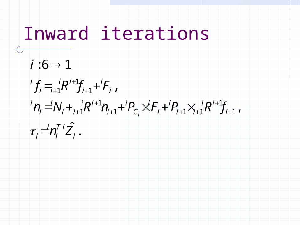
Inward iterations
.ˆ
,
,
16:
11
1111
1
11
1
iiT
ii
i
iii
iii
ii
Ci
iii
iii
ii
ii
iii
iii
Zn
fRPFPnRNn
FfRf
i
i

Inclusion of Gravity Forces
The effect of gravity loading on the links can be included by setting , where G is the gravity vector.
Gv 00

The Structure of the Manipulator Dynamic Equations
: mass matrix
: centrifugal and Coriolis terms
: gravity terms
: matrix of Coriolis coefficients
: centrifugal coefficients
: state space equation
: configuration space
Tn
T
nn
n
nnC
nn
nnnB
GCBM
nG
nV
nnM
GVM
222
21
2
13121
2
,1:
:)(
,12/)1(:
2/)1(:)(
)()()()(
1:)(
1:),(
:)(
)(),()(

Coriolis Force
A fictitious force exerted on a body when it moves in a rotating reference frame.
)(2 vmFCoriolis

Lagrangian Formulation of Manipulator Dynamics
An energy-based approach (N-E: a force balance approach)
N-E and Lagrangian formulation will give the same equations of motion.

Total kinetic energy of a manipulator
Total potential energy of a manipulator
Kinetic and Potential Energy of a Manipulator
n
ii
refCT
ii
n
ii
iii
CTi
iC
TCii
uu
uPgmu
kk
Ivvmk
ii
i
ii
1
00
1
.
,
.
,2
1
2
1

Lagrangian
Is the difference between the kinetic and potential energy of a mechanical system
).(),(),( uk L

vector of actuator torque
The equations of motion for the manipulator
1
n
ukk
dt
d
dt
d
LL

Example 6.5
The center of mass of link 1 and link 2
: variable

Manipulator Dynamics in Cartesian Space
Joint space formulation
Cartesian space formulation
).(),()()(
),(),()(
),(),()(
)(),()(
)(),()(
11
11
GJVJJJMJJMJ
JJJ
JJJ
GJVJMJ
GJVJMJJ
GVM
GVM
TTTT
TTT
TTTT
xxx
XF
X
XX
F
XF

Expressions for the terms in the Cartesian dynamics:
).()()(
,)()()(),()(),(
),()()()(1
GJG
JJMVJV
JMJM
Tx
Tx
TTx

:Coriolis coefficients
:Centrifugal coefficients
The Cartesian configuration space torque equation:
.,1:
:)(
,12/)1(:
2/)1(:)(
),()()()()(
)(),()()(
222
21
2
13121
2
T
n
x
T
nn
x
xxxT
xxxT
n
nnC
nn
nnnB
GCBMJ
GVMJ
X
X

Dynamic Simulation: (Euler Integration)
Nonrigid body effects: friction
: Given initial conditions
.)(2
1)()()(
,)()()(
0,)0(
),()(),()(
),()(),()(
2
0
1
ttttttt
ttttt
FGVM
FGVM
Simulation requires solving the dynamic equation for acceleration
We apply numerical integration to compute positions and velocities:

Next Course:
Amirkabir University of TechnologyComputer Engineering & Information Technology Department
Trajectory Generation


