Manitoba PUB - IEC Load Forecast Final · HVDC High Voltage Direct Current ... The load forecast...

CONF IDENT IAL

DAYMARK ENERGY ADVISORS

370 MAIN STREET, SUITE 325 | WORCESTER, MA 01608

TEL: (617) 778‐5515 | DAYMARKEA.COM

INDEPENDENT EXPERT

CONSULTANT REPORT:

LOAD FORECAST REVIEW

NOVEMBER 15, 2017

PREPARED FOR

Manitoba Public Utilities Board

PREPARED BY

Daymark Energy Advisors

jniemczak

Cross-Out

NOVEMBER 15, 2017

Independent Expert Consultant Report: Load Forecast Review i

TABLE OF CONTENTS

Executive Summary ................................................................................... 1

I. Introduction ......................................................................................... 7

General Rate Application Process and Independent Expert Consultants ..... 7

Organization of this Report ............................................................................ 7

II. Load Forecasting Methodology ............................................................ 9

A. General Overview ............................................................................................ 9

B. Key Sectors ..................................................................................................... 10

1. Residential Methodology ...................................................................................................10

2. Mass Market .......................................................................................................................14

3. Top Consumers ...................................................................................................................17

C. Transmission and Distribution Losses ............................................................ 19

D. Gross Firm Energy and Peak Demand ........................................................... 20

III. Comparison of MH Methodologies with Industry Practice .................. 24

Econometric and End‐Use Forecasting ........................................................ 24

Economic Assumptions ................................................................................ 25

1. GDP Forecasts .....................................................................................................................26

2. Population Forecasts ..........................................................................................................30

Price Elasticity and Implication of Rate Increase ......................................... 32

1. Price Elasticity .....................................................................................................................32

2. Fuel Switching Not Considered ..........................................................................................37

Alternative Load Forecast ............................................................................ 37

1. Sensitivity and Scenario Analysis ........................................................................................38

2. Risk and Uncertainty ...........................................................................................................39

Reliability of Load Forecast .......................................................................... 40

1. Historical Performance of Load Forecasting Methods.......................................................40

2. Accuracy of the Load Forecast ...........................................................................................45

Weather Normalization ............................................................................... 46

NOVEMBER 15, 2017

ii Independent Expert Consultant Report: Load Forecast Review

Incorporation of DSM Savings in Load Forecast .......................................... 48

IV. Load Forecast Changes (2014 to 2017) ............................................... 50

Residential Load Forecast Methodology ..................................................... 51

General Service Mass Market Methodology ............................................... 53

Top Consumers Load Forecast Methodology .............................................. 54

Other Aspects of Load Forecast ................................................................... 56

Assumptions ................................................................................................. 57

V. Summary and Conclusions ................................................................. 60

LIST OF APPENDICIES

APPENDIX A Daymark Energy Advisors’ Scope of Work

APPENDIX B Documents Relied Upon

NOVEMBER 15, 2017

Independent Expert Consultant Report: Load Forecast Review iii

LIST OF TABLES

Table ES1: Key Summary Findings of MH Load Forecast Analysis ................................................... 5 Table 1: MH Estimated Price, Income, and GDP Elasticities ......................................................... 33 Table 2: Estimates of Stepwise Regression Models of Residential Average Usage Model ........... 35 Table 3: Variance Inflation Factor (VIF) of Residential Average Usage Model .............................. 35 Table 4: Estimates of Stepwise Regression of GS Small and Medium Average Usage

Model ................................................................................................................................ 36 Table 5: Estimates of Stepwise Regression of GSMM Large Customers ....................................... 36 Table 6: Sensitivity of Load Forecast to an Assumption Change ................................................... 38 Table 7: Evaluation of Extreme Events .......................................................................................... 39 Table 8: Comparison of MH Estimated Price, Income, and GDP Elasticities in 2014 and

2017 .................................................................................................................................. 58 Table 9: Key Summary Findings of MH Load Forecast Analysis ..................................................... 63

NOVEMBER 15, 2017

iv Independent Expert Consultant Report: Load Forecast Review

LIST OF FIGURES

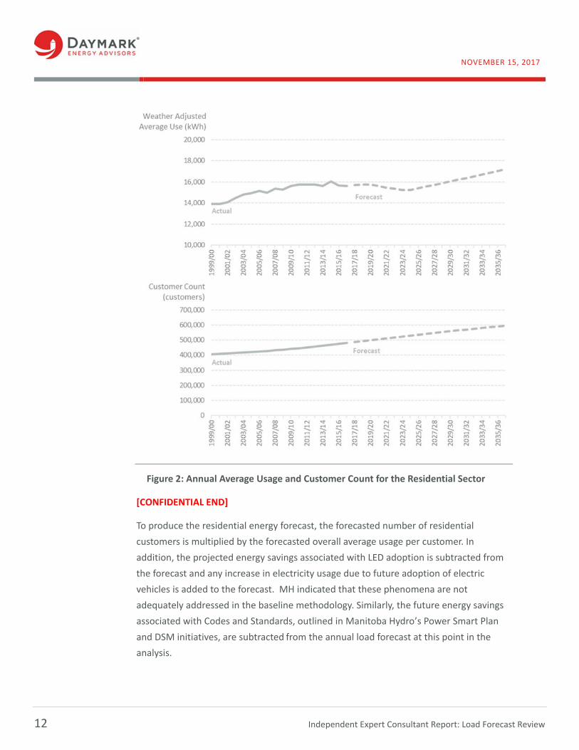
Figure 1. Components of Gross Firm Energy ................................................................................. 10 Figure 2: Annual Average Usage and Customer Count for the Residential Sector ........................ 12 Figure 3: Annual Average Usage and Customer Count for the General Service Mass

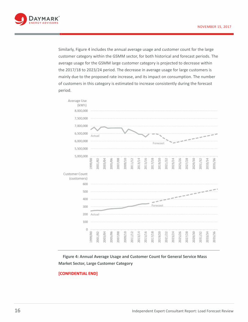
Market Sector, Small and Medium Customer Category ................................................... 15 Figure 4: Annual Average Usage and Customer Count for General Service Mass Market

Sector, Large Customer Category ..................................................................................... 16 Figure 5: Short‐ and Long‐Term Load Forecasts for the General Service Top Consumers

Sector ................................................................................................................................ 18 Figure 6: Gross Firm Energy and Sector‐Level Load Forecasts ...................................................... 21 Figure 7: Monthly Peak Load (MW) for 2017/18 Fiscal Year ......................................................... 22 Figure 8: Annual Peak Demand for MH Service Territory .............................................................. 23 Figure 9: Annual Manitoba GDP (2007 $M) used in MH’s Load Forecast ..................................... 29 Figure 10: Average N‐year Ahead Error Forecast, Population and Residential Customer

Count ................................................................................................................................. 31 Figure 11: Annual Real Electricity Price, Residential Sector (2016/17 = 100) ................................ 32 Figure 12: Comparison of Historical Weather Adjusted Gross Firm Energy (GWh) with

Multiple Forecast Vintages of Gross Firm Energy ............................................................. 41 Figure 13: Comparison of Historical Weather Adjusted Residential Sales (GWh) with

Multiple Forecast Vintages of Residential Sales ............................................................... 42 Figure 14: Comparison of Historical Weather Adjusted General Service Mass Market

Sales (GWh) with Multiple Forecast Vintages of GSMM Sales ......................................... 43 Figure 15: Comparison of Actual General Service Top Consumers Sales (GWh) with

Multiple Forecast Vintages of Top Consumers Sales ........................................................ 44 Figure 16: Comparing Actual and Weather Adjusted Gross Firm Energy with the Annual

Heating Degree Days ......................................................................................................... 47 Figure 17: Annual Gross Firm Energy (GWh) Forecast Comparison .............................................. 50 Figure 18: Annual Gross Total Peak (MW) Forecast Comparison .................................................. 51 Figure 19: Residential Sales (GWh) Comparison between 2014 and 2017 Load Forecasts .......... 52 Figure 20: General Service Mass Market Sales (GWh) Comparison between 2014 and

2017 Load Forecasts ......................................................................................................... 54 Figure 21: General Service Top Consumers Sales (GWh) Comparison between 2014 and

2017 Load Forecasts ......................................................................................................... 56

NOVEMBER 15, 2017

Independent Expert Consultant Report: Load Forecast Review v

LIST OF ACRONYMS

AAGR annual average growth rate

C&S Codes & Standards

CBC Conference Board of Canada

CDD cooling degree days

CSE Centre for Spatial Economics

GDP Gross Domestic Product

GRA General Rate Application (2017/18 & 2018/19)

GSMM General Service Mass Market

GWh gigawatt‐hours

HDD heating degree days

HVDC High Voltage Direct Current

kWh kilowatt‐hours

LSE Load Serving Entities

MH Manitoba Hydro

MW megawatts

PLIL Potential Large Industrial Loads

PUB Manitoba Public Utilities Board

T&D transmission and distribution

VIF variance inflation factor

NOVEMBER 15, 2017

Independent Expert Consultant Report: Load Forecast Review 1

EXECUTIVE SUMMARY

Manitoba Hydro’s (MH) 2017 Load Forecast Report summarizes its approach to

developing a long‐term forecast of energy and peak demand for its system, which it

accomplishes by building up its forecast by sector based on historical econometric

relationships. Daymark Energy Advisors (Daymark) was engaged by the Manitoba Public

Utilities Board (PUB) to provide an independent review of MH’s load forecast. This

report details that review and presents our findings.

Daymark’s scope of work is attached to this report – we were commissioned to gather

sufficient information from available documents, meetings with MH staff, and research

into and knowledge of current forecasting practices to evaluate the reasonableness of

MH’s load forecast methodologies. In addition, a comparison of the 2017 load forecast

to the 2014 load forecast was included in our scope.

MH 2017 Load Forecasting Methodology

Overall, the methodologies employed by MH to develop its projections of future energy

and demand are reflective of industry practice, but are not on the leading edge of

forecasting approaches. MH’s sector‐level, regression‐model‐based load forecast is

consistent with industry practices. Many Load Serving Entities (LSE) typically divide load

forecast analyses into residential, commercial, and industrial sectors and then estimate

the average electricity usage per customer and number of customers in each sector. The

independent variables, or predictors, used in the regression models that MH developed

are similar to the variables used in load forecasts in the industry. MH explicitly

addresses weather impacts on load, savings from DSM and codes and standards, and

load changes associated with electric vehicle adoption, but the company does not

address potential fuel substitution during a time of anticipated large electricity price

increases. MH relies on econometric approaches to a great extent; in this report we offer

several areas of improvement and modification to enhance both the forecast and the

documentation of the company’s process and results.

A key shortcoming of the approach taken by MH is the reliance on a forecast that has a

probability of being accurate 50% of the time – for a business with high capital costs and

long project lead times, a forecast that is expected to address 90% of the potential

futures is typically preferred. In addition, because of the uncertainty and change

prevalent in the energy industry, MH should investigate a diversity of alternative futures

in order to better understand the implications of a range of potential futures in their

long‐term planning process.

NOVEMBER 15, 2017

2 Independent Expert Consultant Report: Load Forecast Review

Key Findings

Table ES1 provides Daymark’s assessment of key topics where improvement in the

methodologies may improve the approach and have an impact on the load forecast used

by MH. Moreover, this table also summarizes MH’s methodology for addressing these

key topics, along with Daymark’s conclusions. We summarize those recommendations

here and provide greater detail throughout this report.

The top consumers forecast relies on a conservative approach to forecasting – MH uses

short‐term knowledge of the MH account executives for particular accounts, which is

useful for the near term, but the long‐term sector projections should rely on all historical

trends and not single out only those accounts with a consistent history of business and

consumption in the province for the duration of the historical data period. In addition,

the changes in methodology between the 2014 and 2017 forecasts for this sector result

in significant forecast differences over the twenty‐year period. The 2017 Potential Large

Industrial Load (PLIL) method used a conservative approach by only considering the total

load of top consumer companies that have been in the MH service territory since

1983/84, thus excluding the historical load of three companies that are currently in the

top consumers sector. Daymark estimated that the conservative PLIL method used in

2017 forecasted 523 GWh less load than would have been forecasted using the 2014

methodology over the forecast period from 2017/18 to 2036/37.

The price elasticities of all three sectors (residential, general service mass market, and

top consumers) reported by MH may be incorrectly estimated. The econometric model

used for estimating residential price elasticity exhibits a multicollinearity issue. Similarly,

the use of trend and dummy variables in the average usage models of both the

residential and general service mass market sectors have suppressed the impact of

electricity price elasticity. In our investigation of the modeling, the regression models

used by MH produced higher price elasticity coefficients before the use of trend or

dummy variables in the sector‐level forecasts. Moreover, the price elasticity estimated

for top consumers through the above‐mentioned conservative PLIL method is lower than

if it was estimated using the PLIL method used in the 2014 load forecast. Although this is

an area of concern, based on the regression parameters, overall R‐square and other

statistics, the overall load forecast of each sector is appropriate in total, the key concern

is in the interpretation of the elasticity coefficients.

The load forecast report provided by MH should include greater attention to the

theoretical basis for their selection of the predictor variables as well as full disclosure

NOVEMBER 15, 2017


and discussion of the potential statistical concerns identified in the analysis so that one

can review the total impact of their decisions as they move to the final forecast.

Price elasticity is included in the regressions used to forecast future energy, therefore

response to price changes are embedded in the modeling. However, the magnitude of

the electricity price increases anticipated are not of the level that have been seen during

the historical period and MH may see greater elasticity impacts than presented in its

2017 load forecast report. Coupled with the multicollinearity issues observed with

regard to the price variable coefficients and the trend and dummy variable impacts, the

forecast could be lower than it is currently predicted by taking a higher price elasticity

coefficient into account.

Finally, MH has historically under‐forecasted population trends, a predictive variable that

underlies the residential and general service mass market forecasts of customer count.

The use of lower customer count forecasts will result in a lower residential load forecast

and a lower general service mass market load forecast.

The possibility of switching to an alternative fuel type or fuel source, driven by increases

in the price of electricity, is not explicitly considered in the MH load forecast analysis. It

is important to consider the potential magnitude of energy source switching that the

proposed MH rate hikes may induce, since electricity prices are requested to increase by

65% in the year 2025 as compared to 2018 rates.1 Similarly, the recent trend of low

natural gas prices and a projected decrease in solar costs may make these alternatives

more economically attractive considering the proposed electricity price changes. It must

also be recognized that a substitution effect will be offset by natural inertia, that is the

consumer effort necessary to change fuels may delay or reduce the potential for

substitution.

Based on our analysis, Daymark has developed the following recommendations for

improving Manitoba Hydro’s current load forecasting methodology:

The load forecast analysis should consider scenario analysis by developing

alternative load forecasts in addition to the base load forecast. These scenarios

would help create alternative future settings that represent the different

possible trends of several key input variables that are used in generating the

base load forecast. Such scenarios could consider key uncertainties by

1 “2017 GCR AT 2017 RATES” excel file provided by MH.

NOVEMBER 15, 2017


representing different assumptions for economic and population growth,

electricity and fuel commodity prices, and CO2 prices.

MH should evaluate the inherent characteristics of fundamental variables using

stochastic risk assessments. Currently, Manitoba Hydro’s method of evaluating

load uncertainty at p10 and p90 levels is based on considering the overall impact

of key input variables on the load variation. Using a stochastic risk assessment

method would allow for the estimating of potential outcomes by incorporating

random variation in the key input variables. Probabilities are assigned to

different values of key uncertain variables that have been identified as such

through sensitivity analysis.

MH may generate a better estimate of weather‐dependent load by using more

than two years of monthly energy and degree day data to estimate the weather‐

dependent relationship. Currently, the company uses two years of data to

estimate the weather‐dependent load relationship and 25 years of data to

define the “normal” weather year. It is unclear at this stage whether this two‐

year‐based coefficient is more extreme than that developed through a reliance

on greater data points, nor is it clear whether the then‐normalized loads are

higher or lower than they should be – but these new normalized loads are the

dependent variables on which the forecast econometric equations are based.

MH should provide greater analysis and information in its next forecast,

providing the rationale for the use of a two‐year coefficient for normalization.

Also, Manitoba Hydro could improve its weather normalization method by using

a shorter period to calculate the “normal” year weather variables.

MH should consider testing its econometric models for a variety of statistical

concerns. For example, the average electricity usage regression models contain

multicollinearity issues. Similarly, MH should consider the economic reasoning

before introducing any new predictor variables into its regression models in

addition to checking the statistical significance, and potential implications for its

price elasticities.

NOVEMBER 15, 2017


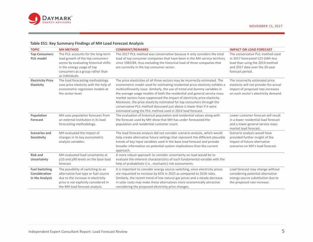
Table ES1: Key Summary Findings of MH Load Forecast Analysis

TOPIC MH METHOD COMMENT/REMARKS IMPACT ON LOAD FORECAST

Top Consumers PLIL model

The PLIL accounts for the long‐term load growth of the top consumers sector by evaluating historical shifts in the energy usage of top consumers as a group rather than as individuals.

The 2017 PLIL method was conservative because it only considers the total load of top consumer companies that have been in the MH service territory since 1983/84, thus excluding the historical load of three companies that are currently in the top consumer sector.

The conservative PLIL method used in 2017 forecasted 523 GWh less load than using the 2014 method and 2017 data over the 20‐year forecast period.

Electricity Price Elasticity

The load forecasting methodology uses price elasticity with the help of econometric regression models at the sector‐level.

The price elasticities of all three sectors may be incorrectly estimated. The econometric model used for estimating residential price elasticity exhibits a multicollinearity issue. Similarly, the use of trend and dummy variables in the average usage models of both the residential and general service mass market sectors have suppressed the impact of electricity price elasticity. Moreover, the price elasticity estimated for top consumers through the conservative PLIL method discussed just above is lower than if it were estimated using the PLIL method used in 2014 load forecast.

The incorrectly estimated price elasticity will not provide the actual impact of proposed rate increases on each sector’s electricity demand.

Population Forecast

MH uses population forecasts from an external institution in its load forecasting methodology.

The evaluation of historical population and residential values along with the forecast used by MH show that MH has under‐forecasted the population and residential customer count.

Lower customer forecast will result in a lower residential load forecast and a lower general service mass market load forecast.

Scenarios and Sensitivity

MH evaluated the impact of changes in its key econometric analysis variables.

The load forecast analysis did not consider scenario analysis, which would help create alternative future settings that represent the different plausible trends of key input variables used in the base load forecast and provide broader information on potential system implications than the current approach.

Scenario analysis would have provided further insight of the impact of future alternative scenarios on MH’s load forecast.

Risk and Uncertainty

MH evaluated load uncertainty at p10 and p90 levels on the base load forecast.

A more robust approach to consider uncertainty on load would be to evaluate the inherent characteristics of each fundamental variable with the help of probabilistic (i.e., stochastic) risk assessments.

Fuel Switching Consideration in the Analysis

The possibility of switching to an alternative fuel type or fuel source due to the increase in electricity price is not explicitly considered in the MH load forecast analysis.

It is important to consider energy source switching, since electricity prices are requested to increase by 65% in 2025 as compared to 2018 rates. Similarly, the recent trend of low natural gas prices and a steady decrease in solar costs may make these alternatives more economically attractive considering the proposed electricity price changes.

Load forecast may change without considering potential alternative energy source substitution due to the proposed rate increase.

NOVEMBER 15, 2017


Load Forecast Methodology Comparison Between 2014 and 2017

Daymark also compared the 2014 and 2017 load forecast methodologies and

assumptions for the various sectors defined by Manitoba Hydro. Overall, the 2017

methods generated a lower long‐term forecast than the analysis conducted in 2014.

Moreover, the annual average growth rate of gross firm energy forecasted in 2017 is

lower than the annual average growth rate forecasted in 2014. The annual average

growth rate of gross firm energy is estimated by using first and tenth year forecast from

both 2014 and 2017 reports. Additionally, the annual growth rate using the ten‐year

gross firm energy forecast was higher in 2014 at 1.46% compared to 0.81% in the 2017

forecast. The key differences between the 2014 and 2017 load forecast methodologies

are in the models used for forecasting general service mass market (GSMM) customer

count, the PLIL method used for capturing long‐term forecasts for the top consumers

category, and economic and population assumptions used in the analysis.

In order to estimate the customer count for the GSMM sector, the 2017 forecast

estimated customer count directly, while the 2014 forecast modeled the percentage

change in the number of customer types. As noted earlier, the 2017 PLIL method used a

conservative approach by only considering the total load of top consumers companies

that have been in MH’s service territory since 1983/84, the start year of MH’s modeling

period. In contrast, the 2014 PLIL methodology considered the load of all companies

included in the top consumers sector.

NOVEMBER 15, 2017


I. INTRODUCTION

General Rate Application Process and Independent Expert Consultants

On May 5, 2017, Manitoba Hydro (MH) filed its 2017/18 & 2018/19 General Rate

Application (GRA). The application has many facets that include interim rate relief and

financial evidence to determine the requested rate increases. A key component in the

financial information provided by Manitoba Hydro is its load forecast.

The Manitoba Public Utilities Board (PUB) retained Daymark Energy Advisors (Daymark)

to review and provide an expert opinion on Manitoba Hydro's export price and revenue

forecasts and electricity load forecasts. This report provides our expert opinion on

electricity load forecasts; Daymark’s expert opinion on export price and revenue

forecasts is provided separately.

Beyond our two expert reports on the above‐mentioned topics, the PUB has also

engaged independent expert consultants to examine and provide opinions on:

1. Updated costs of Manitoba Hydro’s major generation and transmission projects

currently under development or construction;

2. The economic impacts to the Province of Manitoba of proposed electricity rate

increases; and,

3. Capital Projects.

While our report comprehensively addresses the specific aspects of our scope of work,

our review should be considered alongside the other studies and analyses commissioned

by the PUB in connection with Manitoba Hydro’s application.

Organization of this Report This report is organized such that it aligns with our scope of work, which is available on

the PUB’s website2 and is attached to this report as Appendix A, for ease of reference.

Part II, Load Forecasting Methodology, provides our assessment of Manitoba

Hydro’s load forecasting methods, including how they compare to industry

practices;

2 Access available at the following link. http://www.pubmanitoba.ca/v1/proceedings‐decisions/appl‐current/pubs/2017%20mh%20gra/daymark%20iecs%20scope%20of%20work.pdf

NOVEMBER 15, 2017


Part III, Comparison of MH Methodologies with Industry Practices, discusses

Manitoba Hydro’s load forecasting methodologies on key topics and compares

with industry‐practices;

Part IV, Load Forecast Changes (2014 to 2017), provides our review of Manitoba

Hydro’s 2017 Load Forecast and our findings related to how the 2017 forecast

compares to the 2014 forecast used in Manitoba Hydro’s NFAT application; and,

Part V, Summary and Conclusions, bring everything together and describes our

team’s key findings and recommendations.

NOVEMBER 15, 2017


II. LOAD FORECASTING METHODOLOGY

A. General Overview Manitoba Hydro developed sector‐level forecasts to generate its total annual load

forecasts. The key sectors that were modeled separately for generating the overall load

forecast are residential, general service mass market, and general service top

consumers; these sectors form the total consumer sales3.

The total consumer sales, also referred to as general consumer sales, include the energy

supplied to all of Manitoba Hydro’s individually‐billed customers. During the 2016/17

fiscal year,4 MH averaged 570,712 general consumer sales customers, who consumed a

total of 22,025 GWh5 of energy. The common bus is the total load metered at all the

substations in the province that supply MH’s non‐diesel customers. In addition to the

total consumer sales, the common bus includes distribution losses and construction

power. MH reported common bus load to be 23,115 GWh in 2016/17. The common bus

is 1,090 GWh or 4.9% greater than the total consumer sales discussed above.6

MH adds transmission losses and station service load to the common bus load to

calculate the gross firm energy – the total load that needs to be generated for domestic

firm load requirements on the integrated system, excluding diesel customers. MH

reported gross firm energy of 25,227 GWh for 2016/17. This is 3,202 GWh or 14.5%

greater than the total consumer sales. Figure 1 graphically depicts MH’s methodology

for generating the forecast for gross firm energy.

Gross firm energy is then adjusted for DSM‐related energy savings by subtracting

forecasted annual program‐based DSM savings. The DSM‐adjusted annual load forecast

becomes the basis for financial analysis to forecast revenue.

3 “There are four remaining groups of customers. Seasonal customers are those billed twice a year rather than on a monthly basis. Diesel customers are from four remote communities not connected to the integrated grid system. Also included are Flat Rate Water Heating and Area and Roadway Lighting and over 50,000 of these services do not count as customers. The electricity use of these four groups totals 226 GWh or 1.0% of Total Sales.” (Source: Page 2, 2017 Load Forecast Report)

4 The MH fiscal year starts on April 1st of a typical year to March 31st of the following year. For example, 2016/17 represents the period from April 1, 2016 to March 31, 2017. 5 Page 2, 2017 Load Forecast Report. 6 Ibid.

NOVEMBER 15, 2017


Figure 1. Components of Gross Firm Energy

B. Key Sectors

1. Residential Methodology

MH’s residential sector includes a total of 480,365 customers that were responsible for

32.5% of total consumer sales in 2016/17. The residential sector is comprised mostly of

residential structures that include single‐family dwellings, multi‐family dwellings, and

individually‐metered apartment units. MH uses a primary econometric approach to

forecast load for this sector, which is then compared to a secondary approach to support

the reasonableness of the primary approach. Each are described here.

MH’s primary residential forecast methodology, first, estimates two key components:

(1) number of residential customers or dwellings, and (2) the average usage per

residential customer. The customer forecast relies on several third‐party Manitoba

population forecasts and a ratio of total population to total residential customers

estimated by MH. The key assumptions used by the third‐party population forecasts are

summarized in the Economic Assumptions section of this report.

NOVEMBER 15, 2017


To forecast the average annual usage per residential customer, MH uses an econometric

model with assumptions that include electricity prices7, annual disposable income, and

the annual ratio of the number of electric heat customers to total customers. The model

also features a trend variable that, as MH indicates, captures increases in electric use

and house size.8 The average electricity usage, which is the dependent variable in the

regression model, also included both program‐based Codes and Standards DSM savings

and weather adjustments to actual load. [CONFIDENTIAL BEGIN] Figure 2 shows the

annual residential customer average usage and residential customer count for both

historical and forecast periods. The average usage shown in the figure is adjusted for the

change in usage due to weather variation. MH estimates that the average residential

customer usage will decrease slightly for the next few years. The residential customer

count is estimated to increase at a consistent rate during the forecast period.

7 The electricity price variable was lagged by 2.5 years. 8 Manitoba Hydro, "2016 Electric Load Forecast", Market Forecast June 2017, p.62

jniemczak

Cross-Out

NOVEMBER 15, 2017


Figure 2: Annual Average Usage and Customer Count for the Residential Sector

[CONFIDENTIAL END]

To produce the residential energy forecast, the forecasted number of residential

customers is multiplied by the forecasted overall average usage per customer. In

addition, the projected energy savings associated with LED adoption is subtracted from

the forecast and any increase in electricity usage due to future adoption of electric

vehicles is added to the forecast. MH indicated that these phenomena are not

adequately addressed in the baseline methodology. Similarly, the future energy savings

associated with Codes and Standards, outlined in Manitoba Hydro’s Power Smart Plan

and DSM initiatives, are subtracted from the annual load forecast at this point in the

analysis.

jniemczak

Cross-Out

NOVEMBER 15, 2017


MH indicates that it also employed an end‐use forecasting methodology as a secondary

approach to its residential energy forecast. Most of the data to develop these end‐use

forecasts came from the 2017 Economic Outlook and 2014 MH Residential Energy Use

Survey9. The end‐use methodology developed different estimates of the number of both

existing and new dwellings, and the saturation of space and water heating in these

dwellings. The number of space heating systems were forecasted separately in existing

and new dwellings. Specifically, the forecast of space heating systems in new buildings

used econometric models to estimate the number of electric space heating systems in

new single detached and multi‐unit dwellings by region. Separate estimates for space

heating in existing dwellings and water heating systems were developed to forecast the

number of annual replacements using a Weibull distribution10 based on the average age

of the system. Regarding the forecast of water heating systems, MH estimated electric

and natural gas water heater saturations and average age by considering annual

replacements, fuel switching, and saving estimates from the Heating Fuel Choice

initiative11. Moreover, the end‐use forecasting methodology also included the forecast of

electricity usage for other major appliances including central air conditioning, major

appliances, televisions, and lighting by dwelling type.

The total load forecast estimated by this alternative end‐use method, along with

additional information from MH’s 2014 Residential Survey, was balanced against the

load estimated by the primary econometric modeling to ensure that the primary

modeling was reasonable. During discussions with MH, staff indicated that the

secondary modeling confirmed the primary approach and thus no modifications to the

primary approach were needed. However, there was no specific documentation that

described the “balancing” considerations in the load forecast report, nor did it explain

what MH would have done if the load estimated by the primary regression method and

the secondary end‐use method were different. Based on its review, Daymark found that

the secondary end‐use forecasting results were limited in their use by MH, despite the

effort that went into their development and maintenance. Besides balancing, the

secondary end‐use method is also relied upon to estimate the ratio of electric heat

customers to total customers, which is one of the predictors in the primary residential

average usage regression model. However, as discussed later in this report, the use of a

9 MH develops both the Economic Outlook and the Residential End Use Survey and updates them periodically. 10 Weibull distribution is a continuous probability function that is a versatile distribution that can take on the characteristics of other types of distributions, based on the value of the shape parameter. 11 2017 Load Forecasting Methodology, Page 61.

NOVEMBER 15, 2017


“saturation” variable in the primary average usage regression model causes a

multicollinearity issue.

2. Mass Market

The general service mass market (GSMM) sector of MH’s service territory is comprised

of 67,676 customers and was responsible for 42% of total consumer sales in 2016/17. Of

the total GSMM customers, 85% were commercial customers, and the remaining

customers were industrial sector accounts. The 2017 GSMM forecasting methodology

used two different models: one to forecast customer count and the second to forecast

average annual usage, an approach that is similar to the residential modeling

methodology. The GSMM customers were divided into two categories – grouping small

and medium customers in one forecast group and then modeling the larger customers in

a second group.

The method used to forecast GSMM customer counts leveraged econometric models

with assumptions relative to Gross Domestic Product (GDP) and year‐end residential

customer counts. The small and medium customer model used year‐end residential

customer data and Manitoba real GDP from 1985/86 to 2016/17. Similarly, the model

that forecasted large customers used the same year‐end residential customer count and

a blended GDP variable that MH created by combining Manitoba, Canada, and U.S.

GDPs.12

The GSMM average use forecast followed a similar regression method for forecasting

customer count. The average use forecast model for the small and medium customer

category used an econometric model with assumptions related to electricity price,

Manitoba GDP, and a dummy variable, to account for changes in the MH billing system in

2005/06. Similarly, the average use forecast model for the large customer category used

an econometric model with assumptions related to electricity price, the

Manitoba/Canada/U.S. blended GDP, and a dummy variable.13 Both models used

historical annual data from 1989/90 to 2016/17. The use of a lagging time frame with

12 $ ∗ $ ∗ $ where a, b, and c are weights given to different GDP values and the sum of a, b, and c equals to 1. The weights vary by modeled sector. For example, in the regression models used to estimate customer number and average usage for the large GSMM sector, MH used the GDP weights of 30% (a), 35% (b), and 35% (c) for Manitoba, Canada, and US GDP, respectively.

13 The dummy variable from 1999/00 to 2005/06 is included to reflect the average use of the 750V – 30 kV group being higher for during those years by 250,000 kWh. The average usage of large GSMM customers from 1999/00 to 2005/06 is 7,237,157 kWh. The dummy variable used to account for higher usage by 250,000 kWh is just 3.5% of the average usage during that period.

NOVEMBER 15, 2017


the electricity price is inconsistent between the two groups of GSMM categories. The

large customer category relies on an electricity price variable that is lagged by 2 years,

whereas the small and medium customer category regression selected did not lag the

electricity price variable14.

[CONFIDENTIAL BEGIN] Figure 3 shows the annual average usage (kWh) and customer

count for the small and medium customer category within the GSMM sector. The MH

load forecast analysis projects both average usage and customer count to grow slightly

during the forecast period.

Figure 3: Annual Average Usage and Customer Count for the General Service Mass

Market Sector, Small and Medium Customer Category

14 The use of a lagged variable reduces the number of observations used in the regression model. In the load forecast analysis, MH used historical annual data from 1986/87 to 2016/17 resulting in 33 observations. The use of two‐year lag in the large customer category excluded the first three observations resulting in the use of only 28 observations in the analysis.

jniemczak

Cross-Out

NOVEMBER 15, 2017


Similarly, Figure 4 includes the annual average usage and customer count for the large

customer category within the GSMM sector, for both historical and forecast periods. The

average usage for the GSMM large customer category is projected to decrease within

the 2017/18 to 2023/24 period. The decrease in average usage for large customers is

mainly due to the proposed rate increase, and its impact on consumption. The number

of customers in this category is estimated to increase consistently during the forecast

period.

Figure 4: Annual Average Usage and Customer Count for General Service Mass

Market Sector, Large Customer Category

[CONFIDENTIAL END]

jniemczak

Cross-Out

- DAYMARK0

~ ENERGY ADVISORS

NOVEMBER 15, 2017

The final step in forecasting the GSMM total load requires multiplying the forecasted

number of customers in each rate class by the forecasted average use. Similar to the

residential sector, the future use of electric vehicles in the general service mass market

sector was added to this forecast and the energy savings from the codes and standards,

as outlined in Manitoba Hydro's Power Smart Plan, were subtracted from the forecast.

3. Top Consumers The General Service Top Consumers sector of MH's service territory includes

10 companies with 26 separate accounts that represent 26% of total consumer sales in

2016/2017. (CONFIDENTIAL BEGIN] The 10 companies belong to four industry sectors:

primary metals, chemicals, petro/oil/natural gas, and pulp/paper. MH recently moved

seven companies from its top consumers category to the GSMM category, citing that

these companies have smaller annual usage and the usages are consistent over the

future years.

methodology for the top consumers sector involved creating short-term forecasts for

each customer and long-term forecasts for the sector as a whole.

The short-term forecasts were created for each individual customer using information

about the individual companies' (CONFIDENTIAL BEGINS) operating plans, short-term

expansion or contraction plans as shared in the news and in publications, company

prospectuses, and through information gathered by MH's key account representatives.

The company-level short-term forecasts generated the load forecast for the first five

years. The individual company-level forecasts are then held constant beyond year 5 and

a long-term foreFast is considered to account for any changes in the load in the .top

consumer sector as a whole. MH defines this long-term forecast as Potential Large

Industrial Loads (PLIL}.

MH mentioned that the PLIL allows MH to account for the evaluation of historic shifts in

the energy usage of top consumers as a group, rather than as individuals, thus

accounting for unexpected load changes for the "current" companies included in the top

consumers sector. The PLIL method uses an econometric model that fits a regression

model of historical load of the ten top consumer companies with the annual electricity

price and a blended Canadian and U.S.-based GDP assumption.

Figure 5 presents both short- and long-term load forecasts for the Top Consumers sector.

As mentioned before, the short-term forecast covers the first five year of the forecast.


1b

NOVEMBER 15, 2017


The industry‐specific short‐term, along with total short‐term load, are presented from

2017/18 to 2022/23 in the following figure. Beyond 2022/23, in addition to the short‐

term forecast, the figure includes the additional load forecast generated using the PLIL

method.

Figure 5: Short- and Long-Term Load Forecasts for the General Service Top

Consumers Sector

The 2017 PLIL method used a conservative approach by only considering the total load

of top consumers companies that have been in the MH service territory since 1983/84,

the start year of MH’s modeling period. The 2017 PLIL method excluded the historical

load of three companies that are currently in the top consumers sector because they

became part of the category after 1983/84. By excluding the historical load of these

companies, the 2017 PLIL method did not consider the possibility of additional load from

two sources: (1) future new customers that may be joining the MHs service area, nor (2)

additional growth from the three companies that were not part of the group for the

entire historical period. Unlike the 2017 method, the method used in 2014 for

forecasting PLIL load considered the total historical load of the top consumers sector.

Daymark re‐ran MH’s 2017 PLIL model using the method used by MH in 2014,

considering the historical annual load of all companies that are now part of the top

NOVEMBER 15, 2017


consumers sector.15 The exclusion from the 2017 PLIL model of the load of three

companies that became part of the top consumer sector after 1983/84 has at least two

implications. The load forecast estimated for PLIL in 2017 is lower that it would have

been if the method used was consistent with the method used in 2014. For example, the

load forecast associated with PLIL using the 2017 method is 840 GWh in 2036/37 and

the load at the same year using the 2014 methodology is 1,363 GWh. The conservative

PLIL method used in 2017 forecasted 523 GWh less load than the method used in 2014

over the forecast period, a difference of 62%.

Moreover, the electricity price elasticity estimated using the more conservative 2017

methodology is lower by 41% than the price elasticity estimated by using the 2014

methodology16. MH reported the price elasticity impact of ‐0.37 in its 2017 Load

Forecast report. Using MH’s 2014 PLIL methodology, Daymark estimated that the price

elasticity for the top consumers would be ‐0.53. [CONFIDENTIAL END]

C. Transmission and Distribution Losses MH calculated distribution losses by comparing the energy measured at the distribution

centers and the energy measured at combined customers’ meters.17 The annual

distribution losses for MH in the last twenty years has been between 3.5% to 5.5% of

total consumer sales18. MH used distribution losses of 4.6% of total consumer sales in its

load forecast analysis.19

In addition to distribution losses, MH incorporates transmission losses in its load

forecast. MH defined transmission losses as the percentage of power (in terms of total

consumer sales) lost during the transfer of power from generation stations to the

distribution station, collectively known as common bus. The annual transmission losses

for MH have been in the range of 8.8% to 10.5% of total consumer sales in the last 20

15 Daymark’s “Average Use and PLIL stepwise regression summary” spreadsheet.

16 The price elasticity reported in the 2017 Load Forecast Report for Top Consumers is ‐0.3736. Whereas,

Daymark estimated the price elasticity of ‐0.5280 when the 2014 methodology was used with 2017 data.

The difference between the two price elasticities is 41.3% using the calculation:

0.3746 0.52800.3746

∗ 100%

17 MH mentioned that besides technical power lost during transfer, other factors that contributed to losses include the offset tween billing cycle and calendar month, customer accounting adjustments, inaccuracies associated with estimated billing, metered but unbilled consumption of Manitoba Hydro offices, and energy theft (Page 31, 2017 Load Forecast Report). 18 Table 22, Page 31, 2017 Load Forecast Report. 19 Ibid.

jniemczak

Cross-Out

NOVEMBER 15, 2017


years20. In its 2017 Load Forecast Report, MH attributed the transmission losses to the

High Voltage Direct Current (HVDC) lines and the distance over which transmission of

power generated must travel from northern‐located generation to the southern

distribution points. MH used an estimate of 9.1% of total consumer sales to account for

the future transmission loss in its forecast analysis.21 This is the average of the last five

years’ actual transmission losses in the MH territory.

MH’s load forecast analysis then incorporates 13.7% of total consumer sales for its

transmission and distribution (T&D) losses. The percentage of losses considered for T&D

losses is higher than the national averages in Canada and in the U.S. Data from the

World Bank suggests that the average transmission and distribution losses in Canada in

the last ten years is around 8.5%.22 Similarly, the U.S. Energy Information Administration

reports that average transmission and distribution losses in the U.S. for 2015 were

around 4.7%.23

D. Gross Firm Energy and Peak Demand MH uses its sector‐level load forecasts along with distribution losses to estimate the

common bus load forecast. Specifically, the common bus forecast is the sum of total

consumer sales, distribution losses, and construction power. MH adds annual

transmission losses and station service load to the common bus energy to forecast the

gross firm energy. Figure 6 presents the annual forecast of gross firm energy along with

the sector‐level load forecasts presented in the 2017 Load Forecast Report.

20 2017 Load Forecast Report, page 34, Table 25. 21 Ibid. 22 World Bank, accessed October 24, 2017, available at: https://data.worldbank.org/indicator/EG.ELC.LOSS.ZS?locations=CA 23 US Energy Information Administration, accessed October 24, 2017, available at: https://www.eia.gov/tools/faqs/faq.php?id=105&t=3

NOVEMBER 15, 2017


Figure 6: Gross Firm Energy and Sector-Level Load Forecasts

To forecast peak loads, MH breaks the annual energy forecasts into monthly energy

forecasts and applies load factors. To forecast monthly gross firm energy, MH uses

annual Common Bus load forecasts and the average of historical monthly Common Bus

percentages as compared with the annual load. The monthly percentage estimated is

based on the 5‐year monthly percentage of Common Bus to annual Common Bus load.

As shown earlier in Figure 1, the Common Bus is the sum of total consumer sales,

distribution losses, and construction power. The monthly transmission losses and station

service are added to monthly Common Bus to calculate the monthly gross firm energy.

MH then calculated the monthly total peak demand using the monthly gross firm energy

and monthly load factor. Load factor is the ratio of average hourly energy usage to the

peak hourly load. The load factors, and eventually the monthly peak load, are calculated

separately for the Top Consumers sector since the average hourly usage for Top

Consumers is higher relative to their peak value than in the residential of General

Service Mass Market sectors. Top Consumers peak loads are calculated by applying a

92% load factor to that sector’s monthly energy usage. Alternatively, for the residential

and General Service Mass Market customers, a ten‐year historical average load factor

along with the monthly forecasted energy is used to forecast the monthly peak load.

NOVEMBER 15, 2017


Figure 7 shows the monthly peak demand (in MW) for the 2017/18 fiscal year. Please

note that the 2017/18 fiscal year is from April 2017 to March 2018.

Figure 7: Monthly Peak Load (MW) for 2017/18 Fiscal Year

MH has a winter peaking system and, so it estimates the annual peak demand using the

monthly peak demand of three winter months – December, January, and February. MH

also applies a ratio using the January peak to estimate the annual peak demand.24

Figure 8 shows the annual peak demand (MW) of the MH service territory for both

historical and forecast periods.

24 Page 69, 2017 Load Forecast Report.

NOVEMBER 15, 2017


Figure 8: Annual Peak Demand for MH Service Territory

As discussed above, MH uses monthly gross firm energy and monthly load factors to

forecast monthly peaks. While this concept is used by other utilities, it is less popular

compared to other approaches used for forecasting peak load. According to a 2010

survey of utility companies’ forecasting methods conducted by Itron, only 8% of utilities

used this method. The same study found that 59% of surveyed companies were using

econometric modeling and 26% used load shapes to develop the monthly peaks.25

25 Itron “PGE Forecast Review Summary” (April 2015), p.26

NOVEMBER 15, 2017


III. COMPARISON OF MH METHODOLOGIES WITH INDUSTRY PRACTICE

Econometric and End-Use Forecasting As discussed in the Load Forecasting Methodology section, MH performed forecasts at

the sector‐level by dividing its customers into three groups – Residential, General Service

Mass Market, and Top Consumers. MH used econometric regression models to forecast

Residential and GSMM sectors’ average usage per customer and number of customers.

For its Top Consumers category, MH used company‐specific short‐term forecasts along

with an MH‐developed, regression‐based long‐term forecast known as the PLIL method.

MH’s sector‐level, regression model based load forecast is consistent with industry

practices. Load serving entities (LSE) typically divide the load forecast analysis into

residential, commercial, and industrial groups to estimate the average usage and

number of customers in each group. The independent variables or predictors used in

MH’s developed regression models are also similar to the variables used in other load

forecasts in the industry.

One of the key predictor variables used in all the sector‐level forecasts is electricity price,

which allows the utility to account for the potential change in electricity usage with

projected changes in electricity price. Besides electricity price, the regression models

used by MH contained a variable to account for the change in electricity demand with

the change in income or economic health. The Residential sector forecast included real

disposable income per capita, whereas the GSMM sector included a GDP variable.

However, MH did not include any variable to account for fuel substitution, such as

natural gas prices. In light of the electricity price increases due to MH’s proposed rate

increases and the current low natural gas prices, this type of variable should have been

considered.

MH used different approaches for forecasting customer counts for its residential and

GSMM sectors. The customer count forecast for the residential sector is based on a

third‐party population forecast and the ratio of residential customers to population

derived from historical data. Alternatively, the GSMM customer count forecast used

regression models with residential customer count and GDP as predictor variables. As

mentioned, the population and economic forecasts utilized by MH are based on external

organization’s forecasts. We discuss the key assumptions of the external third‐party

forecasts in the Economic Assumptions section of this report.

NOVEMBER 15, 2017


MH also relied on end‐use forecasting in its residential sector load forecast. As discussed

earlier, the use of the end‐use forecasting results was limited, despite the effort used to

develop and maintain the method. The average customer usage derived from the end‐

use method was used only to compare with the average usage estimated from MH’s

econometric method for “reasonableness.” The end‐use method also estimates

“heating saturation”, or the ratio of heating customers to total customers, which is used

as one of the independent variables in the primary regression model that estimates

average usage of residential customers.

Besides the econometric‐based method, utilities have used other modeling approaches

to forecast load, such as time‐series analyses, engineering‐based “bottom‐up”

forecasting approaches, and statistically‐adjusted end‐use modeling.26 The time‐series

models typically use historical sales and weather variables to predict future electricity

load. The econometric regression method, such as the one utilized by MH, can use many

predictor variables including demographic variables, customer usage information,

economy‐related variables, monthly and seasonal‐fixed effects, electricity and other fuel

prices, and weather variables. The engineering‐based “bottoms‐up” approach is an end‐

use based model where the load forecast is estimated by disaggregating the usages of

key end‐uses such as space and water heating, refrigerator, and other appliances or

equipment energy consumption. Statistically‐adjusted end‐use models are a hybrid

structure combining components of the engineering end‐use technology models with

structural econometric equations. In practice, this type of approach mostly considers

three different components: appliance ownership via a saturation component, energy

usage intensity trends of the appliances or equipment, and consumer’s usage behavior.27

Economic Assumptions Economic and population variables are used extensively in the econometric modeling

used to forecast both customer counts and average usage per customer. For example,

the GDP variable is used as one of the predictors for estimating both the number of

customers28 and the average usage for the GSMM sector. Moreover, the PLIL method

that is used to account for the long‐term load forecast of the Top Consumers sector also

26 Carvallo, Juan Pablo and et. al. Load Forecasting in Electric Utility Integrated Resource Planning. Ernest Orlando Lawrence Berkley National Laboratory, October 2016. 27 Ibid. 28 The other predictor used for estimating GSMM customer count is the Residential customer count. And the forecast of Residential customer count is based on the population forecast. Thus, the population forecast has an indirect effect on the GSMM customer count forecast as well.

- DAVMARK. ~ ENERGY ADVISORS

26

NOVEMBER 15, 2017

relies on a combination of the Canada and US GDP as the predictor variable. Similarly,

the load forecast for residential customers is based on the population forecast.

The GDP and population data used in the load forecast models are based on a survey of

forecasts from various financial and consulting institutions. MH used GDP forecasts of

Manitoba, Canada, and United States in its load forecasting methodology by calculating

the simple averages of multiple third-party forecasts. MH has used multiple sources for

its short-term forecast, but relied on only a few for its long-term GDP and population

forecasts. There are many institutions forecasting near-term GDP, whereas there are

only a few institutions that generate a long-term forecast. 29

1. GDP Forecasts [CONFIDENTIAL BEGIN] [L.ebei!iRg #1!5 seetieR es coRjideffHBI 65we1elied en

irtjeffllfltien pF61Rded by MH. Te CORjiffll with MH}

The long-term GDP forecast used by MH is the average forecast of three organizations -

Conference Board of Canada, IHS Economics, and the Centre for Spatial Economics.

Daymark reviewed the method and assumptions used by these three organizations to

generate the long-term GDP forecasts.

The Conference Board of Canada (CBC) provided projections of economic and

population growth for both Canada and Manitoba. At the national level, the CBC

expected the Canadian economy to grow 1.9% in 2017. However, this projected growth

rate is much less than the average increase of 3.2% in the decade before the 2008-2009

recession. The CBC did not expect any acceleration in real GDP growth going into 2018

because of low business investment levels and slowing growth in the labor force tied to

an aging population. Uncertainty pertaining to the rise of U.S. trade protectionism could

also affect forecasted growth. In the long-term, economic growth in Canada is estimated

to average 1.8% from 2019 to 2040. While continued anemic business investment levels

will continue to hamper growth, the aging of Canada's population30 will be the main

reason behind slackening economic growth.31

29 For example, in order to calculate the Manitoba GDP forecast for 2017 and 2018, MH used the average of Manitoba GDP forecast's estimated by CIBC, Desjardins, Laurentian, National Bank, BMO Nesbitt Burns, Royal Bank, Scotiabank, and TD Bank.

I

---------------·---------------------------

Independent Expert Consultant Report: Load Forecast Review

- DAYMARK" ~ ENERGY ADVISORS

NOVEMBER 15, 2017

For the province of Manitoba, the CBC pointed out that the province has experienced

the second-strongest growth of any province over the last 10 years. Manitoba

experienced average annual real GDP growth of 2.5% over the past two decades.

However, CBC argued that the lack of investment in important capital stock will lead to a

decrease in growth in the future years. CBC believes that the province's capital stock

will grow more slowly than most of the other provinces in Canada during the forecast

period.32 CBC expects Manitoba's real GDP growth to average 1.8% annually from 2016

to 2040.

IHS Economics provided a short-term look at the overall Canadian economy and a

medium-term analysis of Manitoba's population and GDP. The short-term forecast for

real GDP growth in Canada was 2.5% for 2017. However, like the CBC analysis, IHS sees

the slowdown in the Canadian labor market and changing trade relations with the U.S.

as potentially affecting economic growth.33 In terms of the U.S. economy, IHS expects

the U.S. economy to grow 2.2% in 2017.34

Regarding Manitoba, the economy of the province grew 2.4% in 2016. This growth was

attributed to growth in goods-producing industries, as well as gains in construction,

manufacturing, and agricultural industries. Growth in construction was greatly helped by

Manitoba Hydro's construction projects such as the Keeyask power generation station

and Bi pole Ill transmission line. There has also been consistent growth of around 2% in

the output in the service sector over the past several years. Because of the closing of the

Thompson nickel mine in October 2017, t he output of the goods-producing industry may

experience some contractionary pressures. Therefore, output growth in this sector could

decrease to 2.1%. In all, Manitoba is expected to experience around 2.2% growth this

year and for the next four years.

The Centre for Spatial Economics (CSE) provides forecasts for economic and population

growth in the U.S., Canada, and Manitoba. For the U.S., real GDP growth is expected to

average 2.1% and 2.3% for the 2017-2021 and 2022-2028 periods, respectively.


- DAYMARK0

'=:I ENERGY ADVISORS

28

NOVEMBER 15, 2017

However, the CSE acknowledged that there is much uncertainty regarding economic

growth globally because of the change in the U.S. administration.35

The economic forecast for Canada has the country's real GDP growing on average 1.9%

annually for 2017-2021and1.7% for 2022-2026. The CSE cited an expected slow

recovery for most commodity prices as an important factor influencing growth since

these prices impact all aspects of aggregate demand. Similar to the CBC's forecast, the

CSE saw a slowing in business investment, especially in the long term when the

investment cycle winds down and major projects are finished. 36 The investment and

spending rates are expected to increase in the long term because of deficit elimination

and the health and social service demands of an aging population. The labor force is

estimated to grow by an average of 0.7% over the medium term. However, this rate will

decrease to 0.6% during the long term as the participation rate declines and the

country's labor force ages. Lastly, the country's population growth is expected to

average 1.0% from 2017-2021and0.9% from 2022-2028.37

Manitoba is expected to see a strong rebound in its manufacturing industry, which will

support its economic growth over the forecast period. The province will see an average

growth in real GDP of 1.8% in the medium term, with continued investment and project

completion in the utility industry helping to bolster this growth during this period.38 On

average, real GDP is estimated to grow 1.2% in the long term.

As discussed earlier, MH calculated the simple average of different third-party GDP

forecasts for Manitoba, Canada, and U.S. regions. Figure 9 shows the annual GDP of the

Manitoba region used in MH's load forecasting analysis for both historical and forecast


NOVEMBER 15, 2017


periods. The Manitoba GDP, expressed in millions of 2007 dollars, is estimated to grow

consistently during the entire load forecast period.

Figure 9: Annual Manitoba GDP (2007 $M) used in MH’s Load Forecast

[CONFIDENTIAL END]

MH uses a single GDP variable, defined as a blended GDP, in its load forecast models

created by geometrically combining Manitoba, Canada, and U.S. GDPs.39 The weights

assigned to each jurisdiction differ based on the sector modeled.40 There are a couple of

issues with the way the blended GDP is created and used in the analysis. First, the GDP

units used for creating a combined GDP for the three sectors are not consistent. MH

used Manitoba’s GDP in millions of dollars ($), whereas Canada and U.S. GDP are

considered in billions of ($). Even though the results (regression coefficients) would not

have changed using the same units for three different GDP, the use of a blended GDP

also has an interpretability issue, especially with the real GDP elasticity. For instance, the

real GDP elasticity estimated for large customers within the GSMM sector is 0.2941 and

39 $ ∗ $ ∗ $ where a, b, and c are weights given to the different GDPs and the sum of a, b, and c equals to 1. The weights vary by modeled sector. For example, in the regression models used to estimate customer number and average usage for the Large GSMM sector, MH used the GDP weights of 30% (a), 35% (b), and 35% (c) for Manitoba, Canada, and US GDP, respectively. 40 The Small, Medium category assigned 100% weight to Manitoba GDP. In the models used for the Large GSMM sector, MH used the GDP weights of 30% (a), 35% (b), and 35% (c) for Manitoba, Canada, and US GDP, respectively. Similarly, the PLIL model assigned equal weights of 50% for Canada and US GDPs. 41 2017 Load Forecast Report, Page 57.

jniemczak

Cross-Out

- DAYMARK. ~ ENERGY ADVISORS

30

NOVEMBER 15, 2017

interpreting this number is challenging until the geometric combination is used to track

back to the individual GDP relationship.

2. Population Forecasts

[CONFIDENTIAL BEGIN] [L6beliRg this seetiel'I 65 Eel'ljidel'lti6! 65 we relied Bl'I

il'l/Bfflf6t561'1 pHJtlided by MH. Fa eel'l/ifm wfth MHJ

With regard to demographics, the load forecasting methodology used by MH relies on

long-term population forecasts from CBC, Spatial Economics, and IHS. CBC concluded

that Manitoba's population is expected to age over the next two decades but at a slower

pace than most other Canadian provinces. A higher birth rate is expected for Manitoba,

which will bolster natural population increases during the forecast period. Additionally,

population growth will be supported by higher levels of international immigration into

the province.

While growth in the labor force is expected to slow down over time in Manitoba, its

forecasted 1% average annual compound growth will be larger than that of any other

province.42 The IHS report mentioned that Manitoba experienced a multi-decadal record

increase in population in 2016 at 1.7%, which would boost domestic demand and labor

force growth. Population growth is forecasted by IHS to generally hover around 1.2% for

the next four years.43 Similarly, the forecast created by Spatial Economics predicts that

the population of the province will grow on average by 1.3% annually in the medium

term while in the long term the growth rate will slow to around 1%. Spatial Economics

expects the increase in net international migration of recent years will decline in the

medium term, but will be offset somewhat by increases in net interprovincial

migration.44

The population forecast forms the basis of both the residential and GSMM sector-level

customer count forecasts. Historically, MH's evaluation of population and residential

customer forecasts shows that MH has typically under-forecasted the population values.

Figure 10 shows the average N-year ahead population and residential customer forecast

errors. MH estimates the forecast errors using their population forecast and the actual

historical numbers. For example, a 5-year ahead error forecast is the percentage

difference between actual population and the forecast for population created 5 years in

·• I

·--------------------------------------


- DAYMARK. ~ ENERGY ADVISORS

NOVEMBER 15, 2017

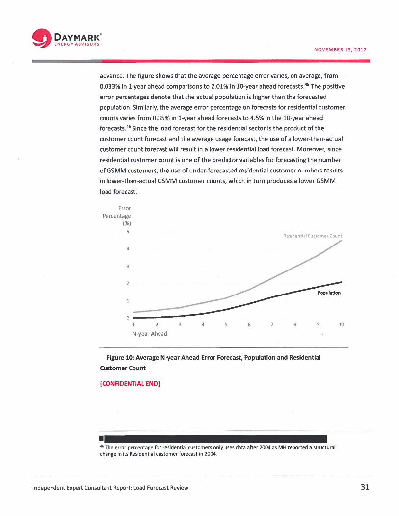
advance. The figure shows that the average percentage error varies, on average, from

0.033% in 1-year ahead comparisons to 2.01% in 10-year ahead forecasts.45 The positive

error percentages denote that the actual population is higher than the forecasted

population. Similarly, the average error percentage on forecasts for residential customer

counts varies from 0.35% in 1-year ahead forecasts to 4.5% in the 10-year ahead

forecasts.46 Since the load forecast for the residential sector is the product of the

customer count forecast and the average usage forecast, the use of a lower-than-actual

customer count forecast will result in a lower residential load forecast. Moreover, since

residential customer count is one of the predictor variables for forecasting the number

of GSMM customers, the use of under-forecasted residential customer numbers results

in lower-than-actual GSMM customer counts, which in turn produces a lower GSMM

load forecast.

Error Percentage

(%} 5

Residential Customer Count

4

3

2

1

0 1 2 3 4 5 6 7 8 9

N-year Ahead

Figure 10: Average N-year Ahead Error Forecast, Population and Residential

Customer Count

(CONFIDENTIAL ENE>]

I 46 The error percentage for residential customers only uses data after 2004 as MH reported a structural change in its Residential customer forecast in 2004.


10

31

NOVEMBER 15, 2017


Price Elasticity and Implication of Rate Increase

1. Price Elasticity

MH has estimated different elasticities by sector to measure and project the economic

effects of electricity price, income, and GDP in the demand for electricity47. The price,

income, and GDP elasticities were estimated from econometric modeling in the sector‐

level load forecasts. It is important to estimate the impact of electricity price on MH

customers’ electricity demand because the proposed rate increase is considerable.

Figure 11 shows the real annual electricity price for residential customers.

Figure 11: Annual Real Electricity Price, Residential Sector (2016/17 = 100)

Table 1 presents the elasticities estimated and reported by MH in its load forecast

report. Using the price elasticity of gross firm energy from the table, MH estimated that

a one percent increase in electricity price reduces the gross firm energy by 0.27%. The

elasticities estimated are then used – along with the future electricity price, income, and

GDP variables – to consider their impact on the load forecast.

47 Price elasticity estimates the impact of a one percent change in electricity demand with a one percent change in electricity price.

NOVEMBER 15, 2017


Table 1: MH Estimated Price, Income, and GDP Elasticities 48

PRICE

ELASTICITY REAL INCOME

ELASTICITY REAL GDP ELASTICITY

Residential Basic ‐0.28 0.30

GS Mass Market Small/Medium ‐0.13 0.55

GS Mass Market Large ‐0.46 0.29

GS Top Consumers ‐0.37 0.62

Gross Firm Energy -0.27 0.10 0.36

Daymark found that some of the elasticities reported by MH may be incorrectly

estimated for different reasons. The econometric model used for the energy forecast

includes a variable that estimates the price elasticity of residential customers and that

coefficient exhibits a multicollinearity issue. MH reported the price elasticity of ‐0.28

using the model with the multicollinearity issue. The regression model used for

estimating average usage per customer has multicollinearity issues mainly due to the

use of highly correlated independent variables ‐ the log transformation income,

saturation, and trend variables are highly correlated with each other. Daymark calculated

the variance inflation factor (VIF) of the independent variables used in MH’s residential

regression model, which assesses how much the variance of an estimated regression

coefficient increases if the predictors are correlated. A VIF value of 5 or greater indicates

a reason to be concerned about multicollinearity49. As presented in Table 3, The VIF

values of the independent variables of income, saturation, and trend variables are

greater than 25 indicating that multicollinearity exists in the model.

Daymark estimated residential price elasticity to be ‐0.34 when the variables causing the

multicollinearity were removed from the equation. Although multicollinearity doesn’t

affect the overall fit of the model, or result in bad forecasts of the dependent variable, it

does produce unreliable coefficient estimates. As a result of the multicollinearity in MH’s

residential average usage model, the coefficients associated with electricity price and

income, which are interpreted as price elasticity and income elasticity, may be

incorrectly estimated50.

Similarly, the price elasticity estimated for the top consumers sector, through the

conservative PLIL method, is lower than it would be if it were estimated using the PLIL

48 2017 Load Forecast Report, Page 57. 49 http://blog.minitab.com/blog/adventures‐in‐statistics‐2/what‐are‐the‐effects‐of‐multicollinearity‐and‐when‐can‐i‐ignore‐them 50 Ibid.

NOVEMBER 15, 2017


method from the 2014 load forecast. MH reported the price elasticity of ‐0.37 for its top

consumer sector in 2017. However, Daymark found that the price elasticity for top

consumers would be ‐0.53 if MH had used the method used in the 2014 Load Forecast

Report.

Moreover, the use of trend and dummy variables in the average usage models may have

suppressed the impact of electricity price elasticity. MH used a trend variable in the

average usage regression model featured in their residential forecast. MH mentioned in

their load forecast methodology that the trend variable was intended to capture

increases in both electric use and house size. A trend variable is typically added to a

regression in order to control for a common trend among the variables51. In the case of

the residential average usage model, a simple positive (1, 2, 3, 4, etc.) trend variable was

added to control for the effects of increasing electric use and house size on the other

regression variables over time. Even though including the trend variable in the average

usage model of residential customer may be justifiable, we found that the residential

price elasticity coefficient, decreases after adding the trend variable.

In order to understand the impacts on price elasticity of the trend and dummy variables

MH used, Daymark performed stepwise regressions by adding independent variables

incrementally to the average usage regressions of residential and GSMM sectors. Table 2

shows the results of the stepwise regression analysis of residential average usage. The

values outside the parentheses are the estimated coefficients while the values inside the

parentheses are the associated t‐values.52 The data in the last column (Model 4) present

the results reported by MH in its 2017 Load Forecast Report53. The values of the

coefficient for electricity price, or the price elasticity of electricity, across different

models becomes smaller in magnitude after the trend variable is included in the

regression equation. The price elasticity decreases from 0.46 (Model 3) to 0.28

(Model 4) once the trend variable is included.

51 For example, regressing a stock price for one company on the stock price of another company may show that they are correlated simply because they were trending in the same direction. By adding a trend variable to the equation, the trend is accounted for and therefore the true nature of the relationship between the two variables is more clearly revealed. 52 A t‐value measures the extremeness of a statistical estimate. It is calculated by subtracting the hypothesized value from the statistical estimate and dividing the resulting value by the estimated standard error. The greater the absolute magnitude of the t‐value from zero, the greater the evidence of statistical significance or difference. 53 2017 Load Forecast Report, Page 62.

NOVEMBER 15, 2017


Table 2: Estimates of Stepwise Regression Models of Residential Average Usage Model

RESIDENTIAL BASIC, AVERAGE USAGE MODEL

Model 1 Model 2 Model 3 Model 4

Electricity Price ‐0.20 (‐0.38) ‐0.34 (‐3.28) ‐0.46 (‐6.82) ‐0.28 (‐4.43)

Income ‐ 0.99 (24.26) 0.23 (1.79) 0.30 (3.19)

Saturation ‐ ‐ 3.42 (6.04) 1.31 (2.12)

Trend ‐ ‐ ‐ 0.01 (4.53)

Adjusted R-Squared ‐0.03713 0.9609 0.985 0.9922

Table 3 presents the variance inflation factor (VIF), which assesses how much the

variance of an estimated regression coefficient increases if the predictors are correlated.

The VIF values associated with the income, saturation, and trend variables in MH’s

residential average usage model show that these three variables created the

multicollinearity issue.

Table 3: Variance Inflation Factor (VIF) of Residential Average Usage Model

RESIDENTIAL BASIC, AVERAGE USAGE MODEL - VIF

Model 1 Model 2 Model 3 Model 4

Electricity Price ‐ 1 1.09 1.84

Income ‐ 1 25.93 26.63

Saturation ‐ ‐ 26.19 60.41

Trend ‐ ‐ ‐ 26.05

Moreover, our analysis shows that the inclusion of dummy variables in GSMM average

usage regressions also reduces the price elasticity. MH included dummy variables in their

forecast models for average usage of GSMM small non‐demand, small demand, and

medium, and large customers.

The dummy variable in the GSMM small and medium customer average usage

model represents a billing system change that resulted in a reclassification of

customers in 2006/07.

The dummy variable in the GSMM large customer average usage model reflects

the average use of the 750V‐30kV group being higher by about 250,000 kWh for

the years from 1999/00 to 2005/06.

NOVEMBER 15, 2017


Dummy variables are often added to regressions in order to represent the measurement

value of a variable that cannot be easily measured on a numeric ratio scale.54 .

However, the coefficients for electricity price (also price elasticities of electricity) in the

GSMM small, medium, and large customer average usage models decrease in magnitude

once the dummy variables are added to each of the regressions. Table 4 presents the

stepwise regression results developed by MH for small and medium customers within

the GSMM sector.

Table 4: Estimates of Stepwise Regression of GS Small and Medium Average Usage Model

GSMM SMALL AND MEDIUM CLASS AVERAGE USAGE MODEL COEFFICIENTS

Model 1 Model 2 Model 3

Electricity Price ‐0.85 (4.17) ‐0.17 (4.13) ‐0.13 (3.61)

Real GDP ‐ 0.46 (29.06) 0.55 (21.57)

Dummy ‐ ‐ 0.03 (3.79)

Adjusted R-Squared 0.3779 0.9814 0.9879

Similarly, Table 5 includes the stepwise regression results for large customers within the

GSMM sector, which were produced by Daymark using the data provided by MH for the

same time period. The decrease in price elasticity shows that including a trend or

dummy variable in the regression equation reduced the forecasted impact of a price

increase compared to when there were no trend or dummy variables used. While the

inclusion of both the trend and dummy variables in MH’s average usage models may be

justified, our analysis shows that the price elasticities reported by MH are

underestimated.

Table 5: Estimates of Stepwise Regression of GSMM Large Customers

GSMM LARGE CUSTOMER AVERAGE USAGE MODEL COEFFICIENTS

Model 1 Model 2 Model 3

Electricity Price ‐1.07 (12.89) ‐0.66 (5.86) ‐0.46 (5.55)

Real GDP ‐ 0.22 (4.35) 0.28 (8.05)

Dummy ‐ ‐ 0.06 (5.63)

Adjusted R-Squared 0.8595 0.9169 0.9627

54 Econometrics, Samuel Cameron, p. 173

NOVEMBER 15, 2017


2. Fuel Switching Not Considered

The load forecasting methodology developed by MH does not consider the effect of

electricity price increase completely, particularly the potential substitution effect of

electricity price increases. Increases in electricity price impacts customers in two

different ways. With the increase in the price of electricity, the budget allocated for

electricity can now only buy fewer units than the consumer could afford before.

Similarly, the increase in electricity price makes the relative price of other substitute

goods cheaper and can reduce the demand for the higher‐priced product (electricity) as

the consumer switches to a lower‐cost substitute product.

The possibility of switching to an alternative fuel type or source due to the increase in

electricity price is not explicitly considered in the MH load forecast analysis. For

example, as the price of electricity increases and the price of natural gas decreases, or

even remains constant, it can be expected that electric load will decrease due to

consumers switching to natural gas as a rational response to the price changes. It is

important to consider the potential magnitude of fuel or source switching that the

proposed rate hike may induce, since electricity prices are requested to increase by 65%

in 2025 as compared to 2018 rates.55 Similarly, the recent trends of low natural gas

prices and a steady decrease in solar costs may make these alternatives more

economically attractive considering the proposed electricity price. It must also be

recognized that a substitution effect will be offset by natural inertia, that is the effort to

change fuels may delay or reduce the potential for substitution.

Alternative Load Forecast The method for developing alternatives or ranges around the base load forecast is an

important step in the forecast analysis because it considers a wider range of future

conditions including alternative trends for the key input variables. A simple point

forecast provides a single view of the future – investigating the potential differences that

could occur using alternatives, or ranges, affords the utility the ability to plan more

effectively by understanding the uncertainties involved.

Investigating alternative load forecast in addition to the base forecast helps to quantify

the additional cost (or benefit) that might be realized if the future load pattern follows

the path specified in the alternative load forecast rather than the base forecast. Thus,

considering these alternative forecasts allows one to understand the magnitude of risk

and uncertainty of different likely future load growth scenarios. The alternative load

55 “2017 GCR AT 2017 RATES” excel file provided by MH.

NOVEMBER 15, 2017


forecasts are mainly developed using economic models based on scenarios or a

statistical (percentile or distribution) approach based on a stochastic approach.

Alternative load forecasts are also developed using percentiles or deviations from the

base forecast as their alternatives. Besides developing alternative load forecast

scenarios, utilities have also evaluated the impact on the base load forecast by varying

key input variables individually which is known as sensitivity analysis.

1. Sensitivity and Scenario Analysis

MH’s load forecast only considered sensitivity analysis by varying the key input variables

of the load forecast analysis. Specifically, MH calculated the impact of a 0.1% annual

change in population, income, GDP, and electricity price, on gross firm energy and peak

demand over the 20‐year forecast period. Table 6 presents these sensitivity results. For

example, MH estimated that a 0.1% higher population growth than forecasted by MH in

their base or reference forecast will increase the energy forecast in by 293 GWh and the

peak load forecast by 54 MW over the next 20 years. The changes in the key input

variables considered in the sensitivity analysis were not based on well‐defined future

economic or technology trends.

Table 6: Sensitivity of Load Forecast to an Assumption Change

CHANGE IN 20 YEAR AVERAGE ANNUAL GROWTH RATE ENERGY (GWh)

PEAK (MW)

0.1% Increase/Decrease in Population 293 54

0.1% Increase/Decrease in Income 49 9

0.1% Increase/Decrease in GDP 178 33

0.1% Increase/Decrease in Electricity Price ∓ 134 ∓ 25

Climate Change per Degree Celsius Warmer 20 ‐ 49

MH also evaluated the impact of a few extreme events on its future energy load. MH

considered the effect of extreme events such as a 100 percent conversion of natural gas

use to electricity, potential changes in load from a very large industrial customer, an

increase in online shopping, high adoption of electric vehicles, and an illustrated effect

of grid parity.56 Table 7 presents the impact of extreme events on the base load forecast

as estimated by MH.

56 Grid parity is when a customer will have an economic option to provide some or all of their electricity need via an alternative energy source. The illustrated example of grid parity used by MH evaluated the load impact due to solar panel installation by 100,000 residential (2 kW system) and 10,000 commercial (50 kW system) customers. (Page 55, 2017 Load Forecast Report)

NOVEMBER 15, 2017


Table 7: Evaluation of Extreme Events

ENERGY (GWh)

PEAK (MW)

All Natural Gas in Manitoba to Electricity 16,000 7,000

Increase/Decrease of One Very Large Industrial Customer 1,500 180

Maximum Potential Effect of Increased Online Shopping – 775 – 143

Additional Load if 100% Electric Vehicle Saturation Rate 12,015 1,502

Illustrated Effect of Grid Parity (e.g., Solar Panels) – 857 – 78

Even though MH evaluated the impact of changes in its key econometric analysis

variables, its load forecast analysis did not consider scenario analysis by developing

alternative load forecasts in addition to the base load forecast. Scenarios help create

alternative future values for key variables that represent the different plausible trends

that could occur. For example, scenarios may consider key uncertainties by representing

different assumptions for economic and population growth, electricity and fuel

commodity prices, and CO2 prices. MH has the ability to develop comprehensive future

forecast values that reflect the interactions of several different fundamental variables

identified from its sensitivity analysis. Moreover, the different trends of key input

variables considered in the scenarios account for the joint impact in the load forecast

and, thus, can be an improved alternative to individual variable’s impacts considered in

the sensitivity analysis.

2. Risk and Uncertainty

MH’s load forecast was created by developing various assumptions and different analysis

methods to estimate Manitoba’s future energy requirement. The underlying variations

in the fundamental variables such as population and economic outlook, Top Consumer

customers, and overall usage pattern gives rise to uncertainty inherent in MH’s load

forecast, as it does in any projection. MH created a P50 load forecast, meaning there is

an expectation of a 50% chance that the actual growth will be higher than the forecast,

and a 50% chance that the actual growth will be lower than the forecasted growth. In

order to evaluate the potential load variation, MH then created two different load

growth scenarios by considering a P10 and P90 of the base load forecast.57 The P90 load

forecast denotes the level of annual electricity load that is forecasted to be exceeded

90% of the year. The P10 and P90 load forecasts estimated by MH considered the

variability due to long‐term economic effects and did not include variability due to

57 High (Low) Load = Base Forecast +/‐ 1.28*Standard Deviation

NOVEMBER 15, 2017


weather.58 The load forecast variability estimated at p10 and p90 are not utilized further

in the load forecast analysis.

MH’s method of evaluating load uncertainty at p10 and p90 levels relied on considering

the overall impact of key input variables such as population, economy, and other effects

on the load variation. Utilities have also utilized a more robust approach by evaluating

the inherent characteristics of each fundamental variable with the help of probabilistic

(i.e., stochastic) risk assessments. This method provides a tool for estimating potential

outcomes by allowing random variations in one or more key input variables.

Probabilities are assigned to different values of the key uncertain variables, preferably

identified through sensitivity analysis. The random variations can be based on

fluctuations observed in historical data using standard time‐series techniques.59

Outcomes are then identified that are associated with different values of the key factors

in combination. Since the probabilistic method involves generating multiple outcomes

by varying key input variables, the final results often include the expected outcome and

a probability distribution for these key factors.

Reliability of Load Forecast Daymark compared MH’s load forecast from previous years with the actual load to

assess the reliability of the load forecast created by MH. Daymark also reviewed MH’s

method of calculating the accuracy of its load forecast by comparing actual weather

adjusted load with the forecasts created five‐ and ten‐years in advance.

1. Historical Performance of Load Forecasting Methods

Daymark gathered forecasts of gross firm energy and sector‐level loads created in 2011,

2014, 2015, and 2016 with the goal of comparing these forecasts with the actual

observed load.60 Specifically, we compared the historical actual gross firm energy,

residential load, GSMM load, and top consumer load to the corresponding forecasts

conducted by Manitoba Hydro through the years. Additionally, weather adjusted values

were compared to actual energy values; these are also shown in the coming figures.

58 The 2017 Load Forecast Report mentioned that the standard deviation of weather variation has been found to be approximately 2% of both energy and peak. Annual weather variations tend to be independent of the economy, so the variance due to weather can be added to the economic variance to derive an overall combined variance. (Source: 2017 Load Forecast Report, Page 44). 59 The random variations of the input variables are then used to generate a distribution of potential outcomes from a large number of simulations. 60 “Electric Load Forecast 2011”, “Electric Load Forecast 2014”, “Electric Load Forecast 2015”, “Electric Load Forecast 2016”.

NOVEMBER 15, 2017


Figure 12 compares historical weather adjusted gross firm energy to different forecast

vintages of gross firm energy. Comparing the 2011, 2014, and 2015 forecast values of

the gross firm energy with the weather adjusted actual gross firm energy, this figure

demonstrates that the forecasted load was greater than the actual load for all years. In

particular, the 2011 forecast has the highest estimated deviations, followed by the 2015

and the 2014 forecasts. Only one historical data point exists for the 2016 forecast.

Figure 12: Comparison of Historical Weather Adjusted Gross Firm Energy (GWh) with

Multiple Forecast Vintages of Gross Firm Energy

NOVEMBER 15, 2017


Figure 13 displays the estimated residential sales load values from the various forecasts

conducted by MH. The 2011 forecast has consistently higher values than the actual

historical adjusted values. The 2015 forecast also estimated higher values than those in

2017 in the later years shown in the figure. The figure shows that the Residential

forecast created in 2014 estimated lower load than actual for the first two years of the

forecast.

Figure 13: Comparison of Historical Weather Adjusted Residential Sales (GWh) with

Multiple Forecast Vintages of Residential Sales

NOVEMBER 15, 2017


Figure 14 shows the estimated GSMM load values from the different forecast years.

Overall, each forecast estimated load values that were higher than actual adjusted

energy values. The only exception was the 2016/17 value from the 2015 forecast, which

was slightly lower than the actual forecast.

Figure 14: Comparison of Historical Weather Adjusted General Service Mass Market

Sales (GWh) with Multiple Forecast Vintages of GSMM Sales

NOVEMBER 15, 2017


Figure 15 displays the estimated GS top consumer load from different MH forecasts.

While all the previous forecasts have load values that were higher than actual historical

consumption, there is significant variability in different years’ forecasts from 2015/2016.

While the 2015 forecast value is lower than both the 2011 and 2014 forecast value in

2015/16, it exceeds both the 2011 and 2014 values by 2016/17. The 2014 forecast value

rises to more or less equal the 2011 forecast value in 2015/16 but falls below the 2014

forecast again by 2016/17.

Figure 15: Comparison of Actual General Service Top Consumers Sales (GWh) with

Multiple Forecast Vintages of Top Consumers Sales

NOVEMBER 15, 2017


2. Accuracy of the Load Forecast

MH calculates the accuracy61 of its previous forecast by comparing the actual load with

the forecasts created five‐ and ten‐years in advance. Manitoba Hydro acknowledged that

only a certain degree of accuracy is possible regarding the load forecasts due to load

variation caused by both population and economic growth.62 The Company estimates

that there is only an 80% chance that a 5‐year energy forecast will fall within 3.2% of the

actual and an 80% chance that a 10‐year forecast will be within 4.3% of the actual due to

economic variability alone. The Company tracks historic forecast variation because of

these forecast uncertainties63.

The accuracy calculation method used by MH depends on weather normalization and on

adjustments that are made to the forecast by subtracting program‐based DSM savings.

First, the actual, observed load is weather adjusted. Second, the forecasted program‐

based DSM savings are subtracted from the accuracy calculation. There is no analysis

with regard to how forecasted program‐based DSM savings compares with the actual

savings. Thus, weather normalization and handling of program‐based DSM affects the

load forecast accuracy that MH is estimating.

MH can use additional methods to analyze its load forecast accuracies. For example, the

sum of errors and annual average growth rate (AAGR) can be alternative metrics to

compare forecasts with actual load.64 The sum of errors is the ratio of the difference

between forecasted and actual load to the actual load for any given year. The annual

average growth rate65 compares the load growth rate between two years of actual and

forecasted load.

61 Accuracy at five‐year prior: / where is observed

load ± weather adjustment – cumulative program‐based DSM savings of five years.

62 2017 Load Forecast Report, Page 47. 63 Ibid. 64 Hyndman, R., 2006. Another Look at Forecast Accuracy Metrics for Intermittent Demand. Foresight Int. J. Appl. Forecast. 43–46. http://citeseerx.ist.psu.edu/viewdoc/download?doi=10.1.1.218.7816&rep=rep1&type=pdf 65 ∗ 1

NOVEMBER 15, 2017


Weather Normalization MH assumes that its load forecast is adjusted to reflect what is considered to be normal

weather. The historical annual loads are adjusted to account for weather variability

within its load forecasting process. MH adjusts actual load for any weather‐dependent

usage due to actual differences in weather patterns in the current year as compared to a

‘normal’ weather pattern year. MH defined the ‘normal’ weather by using a 25‐year

rolling average monthly temperature. This process, commonly known as weather

normalization, adjusts consumption for the weather‐dependent load overserved in the

actual load data. A common method in weather normalization, also used by MH, is to

first quantify the electricity demand that is dependent on weather being colder or hotter

than normal temperature days.66

MH’s weather normalization regression models used the monthly energy usage, actual

heating degree days (HDD), and cooling degree days (CDD) for the same month for the

previous two years (24 data points). MH then used the resulting regression coefficients

with ‘normal’ CDD and HDD data to calculate the weather‐dependent energy usage for

that year. The ‘normal’ degree days are based on the 25‐year rolling temperature

average of the Manitoba region.

Figure 16 compares the actual historical gross firm energy with weather adjusted gross

firm energy along with the annual HDDs67 during the same period. The weather adjusted

annual gross firm energy is lower than actual gross firm energy since actual annual HDDs

are lower than the normal HDD. Similarly, the weather adjusted load is greater than

actual gross firm energy when the annual HDDs are higher than normal HDDs.

66 The parameters used to measure weather‐related electricity consumption are degree days. The degree days assume that consumers use more or less energy when the temperature is above or below a certain base temperature. MH has used a base temperature of 14˚C to calculate the heating degree days (HDD) and used the base temperature of 18˚C to calculate the cooling degree days (CDD). 67 The annual HDDs were calculated using monthly Common Bus HDDs used by MH in its weather normalization. The HDDs are expressed in terms of fiscal year. For example, annual HDDs of 2016/17 includes total monthly HDDs from April 2016 to March 2017.

NOVEMBER 15, 2017


Figure 16: Comparing Actual and Weather Adjusted Gross Firm Energy with the

Annual Heating Degree Days

MH may get better estimates of weather‐dependent load by relying on more than two‐

years of monthly energy and degree days to estimate the weather‐dependent

relationship.68 Regression models usually produce robust estimates when more data

points are used. Since there is wide variation in recent weather patterns, the use of

more monthly observation in the weather normalization model will help improve the

68 Introduction to Regression Analysis, Nonlinear Regression and Curve Fitting: http://www.nlreg.com/intro.htm

NOVEMBER 15, 2017


robustness of weather dependent estimates. Daymark re‐produced the regression

results by using the previous ten years of monthly energy usage and weather data using

the same weather normalization modeling parameters used by MH. The use of 10‐year

monthly usage and weather data for residential usage produced lower CDD and HDD

coefficients than the coefficients estimated by MH’s use of two years of data.69

MH could also improve its weather normalization by using a shorter‐period to calculate

the “normal” year weather variables. As mentioned earlier, MH used a 25‐year rolling

average to get normal year weather parameters for CDD and HDD. Many utilities are

moving to the use of shorter time‐periods to create normal weather temperature

profiles. For example, BC Hydro uses a ten‐year rolling average of monthly heating and

cooling degree days.70 With the climate change debate, it may make sense to use a

shorter time‐frame if in fact electricity use is becoming more weather‐dependent.

However, MH has not provided evidence to demonstrate why one approach is superior

to the other.

Incorporation of DSM Savings in Load Forecast MH considered two potential DSM‐based savings programs in the load forecast analysis:

savings based on the implementation of Codes and Standards (C&S) and utility program‐

based DSM savings. The annual historical average electricity usage also included both

program‐based and C&S‐based energy savings. Essentially, MH added back historic DSM

savings to the actual measured energy use prior to estimating its average use per

customer for residential, GSMM, and top consumers71 sectors.

The logic for including these DSM savings with actual measured MH load is that MH

would have to serve this additional load if the DSM measures were not in place as part

of C&S or utility‐sponsored DSM programs. However, it is not clear why MH would add

DSM savings related with C&S savings. The C&S DSM savings are based on set rules and

these rules may have the same requirements going forward if they are not replaced by

more stringent rules. Even though MH excludes the future C&S savings once the

forecasts are created, the use of historical C&S DSM savings in the average usage

regression model estimates different future average usage values than the average

69 Using the same regression model used by MH with 10‐year data. Data provided by MH in excel workbook: “WeatherNormalizationUpdated2‐Daymark.xlsx” 70 BC Hydro, Fiscal 2017 to Fiscal 2019 Revenue Requirements Application, Chapter 3‐Load and Revenue Forecast, Page 3‐6. 71 The DSM savings are adjusted via PLIL model for Top Consumer category.

NOVEMBER 15, 2017


usage regression model used by MH by considering both C&S and program‐based DSM

savings.

Comparing MH’s DSM forecasting method to those used by other utilities, a 2013 survey

of utility forecasting methods found that 38% of utilities surveyed subtract DSM savings

from their forecast.72 Like the method used by Manitoba Hydro, this method assumes

that current DSM program impacts are already accounted for in the forecast in the

historical data and future DSM programs are not included and therefore are subtracted.

Around 22% of utilities surveyed estimate a model with historical DSM and then subtract

past and future DSM savings, while 11% of those surveyed capture DSM impacts through

the SAE model specification.

72 Itron “2013 Forecasting Benchmark Survey” p.20

NOVEMBER 15, 2017


IV. LOAD FORECAST CHANGES (2014 TO 2017)

Daymark carried out a comparison of the 2014 and 2017 load forecast methodologies

and assumptions for the various customer groups defined by Manitoba Hydro. These

customer group methodologies included the residential basic methodology, the general

service mass market methodology, and the general service top consumer methodology.

Similarly, we also compared the economic and population assumptions used in

generating both the 2014 and 2017 load forecasts.

Overall, the methods used in 2017 produced lower long‐term forecasts than the

analyses performed in 2014. Figure 17 shows the gross firm energy forecasts created

during 2014 and 2017. The 10‐year historical growth rate of gross firm energy is 0.85%.

The gross firm energy forecasted during 2017 is lower as compared with the gross firm

energy forecasted during 2014. The annual growth rate using ten‐year gross firm energy

forecasted in 2014 is 1.46%. Whereas, the annual growth rate using the 10‐year forecast

from the 2017 methodology is 0.81.

Figure 17: Annual Gross Firm Energy (GWh) Forecast Comparison

NOVEMBER 15, 2017


Similarly, Figure 18 shows the comparison of MH’s 2014 and 2017 peak load forecasts.

Consistent with the gross firm energy trend, the MH forecast of peak load in 2017 is

lower than the peak load forecasted in 2014.

Figure 18: Annual Gross Total Peak (MW) Forecast Comparison

Residential Load Forecast Methodology An econometric forecast of the average annual electricity use per customer of the

residential basic sector was featured in both the 2014 and the 2017 methodologies.

Although both the 2014 and 2017 forecasts used trend variables in their models, the

trend variable used in the 2017 forecast was specifically defined as capturing increases

in electric use and house size.73 Lastly, the forecasted number of dwellings, multiplied by

the overall average customer usage determined the GWh forecast in both 2014 and in

2017. However, the 2014 forecast mentions that annual savings estimates from the

Heating Fuel Choice Initiative were subtracted whereas the 2017 forecast subtracted

energy savings tied to the higher‐adoption of LED lights.

Figure 19 shows the annual residential load forecasts estimated in 2014 and 2017. The

residential load forecast is quite comparable between 2014 and 2017, although MH

73 Manitoba Hydro, "2017 Electric Load Forecast", Market Forecast June 2016.p. 62.

NOVEMBER 15, 2017


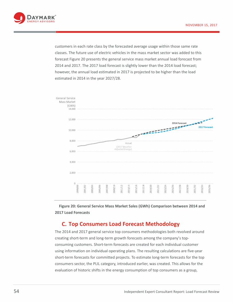
estimated a slightly lower forecast for the residential sector customers in 2017 than in

2014, perhaps as a result of the elasticity response to anticipated electricity price

increases among other factors.

Figure 19: Residential Sales (GWh) Comparison between 2014 and 2017 Load

Forecasts

In addition to the econometric model for average usage, the residential load forecast

included end‐use forecasting in both 2014 and 2017. However, it is not clear how end‐

use forecasting methodology is further used in both year’s load forecasts, besides its use

in estimating the ratio of electric heat customers to total customers, which is used in the

average usage regression model.74 The information used for the end‐use forecasting

model used information provided by the residential energy use survey. The 2014

methodology used the 2009 residential energy use survey while the 2017 methodology

used the residential survey completed in 2014. The end‐use forecasting methodologies

used in 2014 and 2017 varied in forecasting the number of existing residential

74 The ratio is expressed as a “Saturation” variable in the 2017 Load Forecast report. The 2017 report also mentioned the use of end‐use forecasting results to check the reasonableness of total usage estimated from the average usage regression model. However, it is not clear how MH would adjust the average usage model if the results from the regression and end use models provided different results.

NOVEMBER 15, 2017


dwellings75, space heating systems in the new dwellings76, assumptions used for existing

heating system in 2014, and heating choice method for 201777 .

General Service Mass Market Methodology The general service mass market methodology in both 2014 and 2017 used two

forecasts: a customer count forecast, and an average customer usage forecast. The

customer count forecast model uses econometric regressions in both years. However,

there are some differences between how this analysis was carried out in 2014 as

compared to 2017. The percentage change in the number of customers was modeled in

2014 while the 2017 forecast estimated the customer count directly. Furthermore, the

variable for Manitoba GDP is explained as being lagged78 in the 2014 analysis but not in

the 2017 analysis. Depending on the customer class, the GDP and customer variables

used in the model equations for GSMM large customers differ between 2014 and 2017.

The 2017 methodology uses a blended GDP variable created by blending Manitoba,

Canada, U.S. real GDPs to forecast the year‐end number of GSMM large customers. We

discussed the implication of using a blended variable in detail in the GDP Forecasts

section of this report.

The general service mass market average usage forecast calculated the historical average

use per general service customer. The 2014 model does not lag electric price while the

2017 model lags electric price by two years. Unlike the 2014 model, the 2017 model

incorporates dummy variables. The 2017 model also used a blended real GDP and holds

the average use of each rate group constant. Finally, the 2017 model adjusted the

number of customers in each group. The general service mass market sales forecast for

2014 and 2017 both project total GWh by multiplying the forecasted number of

75 The forecast for existing dwellings differed between the 2014 and 2017 residential basic methodologies since the 2017 methodology specifically mentions that customer space heating fuel switches were taken into consideration for the forecast. The treatment of historical space heating systems by dwelling did not differ between the two methodologies, both involving the division of historical dwellings by type and region into nine space heating systems. 76 The regions featured in the forecast were “Winnipeg” and “South Gas” in 2014 while the 2017 regions included “Winnipeg” and “Gas Available.” The regressions in the 2017 forecasts used a natural gas price trend variable, which was absent in the 2014 regressions. The weighted average and lag‐years used in the regressions differ between 2014 and 2017. It seemed that choice of lag variables and assigned weighting is mainly driven with the goal of getting optimum statistical results rather than economic sense. 77 The 2014 forecast methodology mentions that the former heating systems of I DON’T KNOW WHAT THIS MEANS??? dwellings were determined from billing system notes and inventory, while the 2017 forecast methodology makes no mention of this technique. The utilization of saving estimates from the Heating Fuel Choice initiative was also mentioned in the 2017 methodology for the forecast of water heating systems in new and existing dwellings but missing in the 2014 methodology. CLARITY PLEASE 78 The lagged independent variable (Manitoba GDP) allows the regression to account for the impact of past value of the independent variable on the current dependent variable.

NOVEMBER 15, 2017


customers in each rate class by the forecasted average usage within those same rate

classes. The future use of electric vehicles in the mass market sector was added to this

forecast Figure 20 presents the general service mass market annual load forecast from

2014 and 2017. The 2017 load forecast is slightly lower than the 2014 load forecast;

however, the annual load estimated in 2017 is projected to be higher than the load

estimated in 2014 in the year 2027/28.

Figure 20: General Service Mass Market Sales (GWh) Comparison between 2014 and

2017 Load Forecasts

Top Consumers Load Forecast Methodology The 2014 and 2017 general service top consumers methodologies both revolved around

creating short‐term and long‐term growth forecasts among the company’s top‐

consuming customers. Short‐term forecasts are created for each individual customer

using information on individual operating plans. The resulting calculations are five‐year

short‐term forecasts for committed projects. To estimate long‐term forecasts for the top

consumers sector, the PLIL category, introduced earlier, was created. This allows for the

evaluation of historic shifts in the energy consumption of top consumers as a group,

- DAYMARK" ~ ENERGY ADVISORS

NOVEMBER 15, 2017

rather than sirnply as individuals. The differences between the 2014 and 2017 methods

dealt with the number of companies included in the individual short-term forecasts. The

2014 method relied on 17 individual company forecasts while the 2017 method relies on

just 10 individual company forecasts. This is because the 7 other companies moved to

the general service mass market category. [CONFIDENTIAL BEGIN]

[CONFIDENTIAL END]

The long-term PLIL forecast used the same econometric model in both 2014 and 2017.

However, the 2017 PLIL method used a conservative approach by only considering the

total load of top consumer companies that have been in MH's service territory since

1983/84, the start year of MH's modeling period. The detailed discussion regarding the

impact of PLIL method change in 2017 on MH load forecast is presented in the earlier

Top Consumers section of this report. Figure 21 shows the load forecast comparison

between 2014 and 2017 for the top consumers sector. Besides the short-term load

forecast differences (number of companies included in top consumer category), the

decrease in 2017 load forecast is also a result of the change in the PLIL long-term

forecasting method in the 2017 load forecast.


1b

NOVEMBER 15, 2017


Figure 21: General Service Top Consumers Sales (GWh) Comparison between 2014

and 2017 Load Forecasts

Other Aspects of Load Forecast The methodology for forecasting electric vehicles was the same in both 2014 and 2017.

This forecast relied on historical automobile registrations per year in Manitoba to aid in

estimating future trends.

The 2014 and 2017 methodologies for forecasting the individual communities that were

supplied by diesel generation were also the same. In order to forecast monthly gross

firm energy, the 2014 and 2017 methodologies averaged both the monthly percentages

of customer growth through the year and the GWh for the month of the year for a

specific time period. This time‐period was three to five years in the 2014 methodology

and five years in the 2017 methodology.

The calculation of monthly and annual gross firm energy and gross total peak in 2014

and 2017 were the same except for a few aspects. The 2014 method added top

consumer peaks using a 95% load factor applied to the top consumer monthly energy

while the 2017 method used a 92% load factor. While both the 2014 and 2017

methodologies used a three‐month winter load factor for the winter months of

NOVEMBER 15, 2017


December, January, and February to calculate the annual gross total peak, the 2017

method applied a ratio from the January peak for use as the annual peak.

Assumptions The economic assumptions that went into the 2014 and 2017 load forecast were taken

from Manitoba Hydro’s economic outlook and energy price outlook for those respective

years. The number of residential basic customers in Manitoba was forecasted to increase

by 1.3% (5,802 units) in 2014/2015 with averages of 1.0% per year throughout the

forecast period. The historical average increase in 2014 was 1.0% per year over the last

ten years. In 2017, the forecast of the number of residential basic customers estimated a

1.2 % increase in 2017/18 with an annual average of 1.1% per year during the forecast

period. For 2017, the historical average increase in customers was 1.2% per year over

the last ten years.

The electricity price forecast in both 2014 and 2017 is based on the Consumer Price

Index and rate increase projections from the integrated financial forecast. In 2014, the

real electricity price was forecasted to increase by 2.2% in 2014/15, increase between

1.9% and 2.1% from 2015/16 to 2018/19, and increase by 1.9% annually for the

remainder of the forecast period79. In 2017, the price was forecasted to increase 3.36%

in 2018, 7.9% annually from 2019 to 2024, and 4.54% in 2025.80 In addition, MH also

included a 2% price increase beyond 2025 to adjust for inflation.

In 2014, the real Manitoba disposable income annual growth was 1.2% for the previous

10 years and 0.8 % for the previous 20 years. The rate was forecasted to grow at 1.0%

annually for the following 10 years and 1.2% annually for the next 20 years. These values

changed in 2017, with the disposable income per residential customer growing on

average by 1.4% during the past 20 years and 1.7% over the past 10 years. The

disposable income is forecasted to grow 0.6% annually for the next 20 years and was

used in the residential basic forecast in both 2014 and 2017.

Forecast information on the real economic growth (GDP) in Manitoba is used in the

general service mass market and general service top consumers forecasts. The 2014

forecast expected estimated economic growth to be 2.2% in 2014/15, with 2.7%

expected growth by 2016/17. Growth was then estimated to drop to 1.6% by 2020/21,

staying level for the rest of the forecast period. In the 2017 methodology, the real

economic growth expectations for Manitoba, Canada, and the U.S. that were used in the

79 2014 Load Forecast Report, Page 56 80 MH‐provided Excel workpaper. “2017 GCR AT 2017 Rates”

NOVEMBER 15, 2017


analysis were different than the numbers used in 2014. The real Manitoba GDP is

expected to grow 2.0% in 2017/2018 and an average of 1.6% annually for the next 20

years. GDP in Canada is forecasted to grow 2.1% in 2017/18 and an average of 1.8%

annually over the next 20 years. The GDP for the U.S. is estimated to grow 2.3% in

2017/18 and an average of 2.1% annually for the next 20 years.

The elasticities of price, real income, and real GDP were estimated using econometric

modeling in the 2014 and 2017 forecasts. Price elasticities were determined for

residential basic customers, general service mass market small and medium customers,

general service mass market large customers, general service top consumers customers,

and gross firm energy. Real income elasticities were calculated for residential basic and

gross firm energy categories. Lastly, real GDP elasticities were estimated for all general

service customer categories. Table 8 presents the price, income, and GDP elasticities

estimated by MH in its 2014 and 2017 Load Forecast report. The elasticities estimated

are very similar in both years.

Table 8: Comparison of MH Estimated Price, Income, and GDP Elasticities in 201481 and 201782

2014 Load Forecast Methodology

PRICE







Gross Firm Energy -0.25 0.51

(Income + GDP Combined)

2017 Load Forecast Methodology

PRICE







Gross Firm Energy -0.27 0.1 0.36

812014 Load Forecast Report, Page 58.

NOVEMBER 15, 2017


Both the 2014 and 2017 forecasts reflected future DSM savings that were tied to existing

provincial building codes and improved equipment efficiency standards (codes and

standards). These DSM‐associated savings from programs are included in the historical

data used in the forecast. It is explained in the 2014 forecast that codes and standards

were treated as a supply‐side resource and are accounted for in Manitoba Hydro’s

power smart plan and not in the forecast. The 2017 forecast mentions that future DSM

savings from future power smart offerings above the current level and incremental to

the codes and standards were subtracted from the load forecast.

The normal weather assumptions for both 2014 and 2017 are based on degree days

used to measure weather for the forecast. The temperatures used are from Winnipeg

and are expressed in Heating Degree Days (HDD) and Cooling Degree Days (CDD),

respectively. The HDD are the number of average degrees colder than 14 degrees C each

day, whereas the CDD are the number of average degrees warmer than 18 degrees C

each day. The forecast assumes normal weather, which is determined from a 25‐year

average of HDD and CDD in Winnipeg. This 25‐year period was April 1989 to March 2014

for the 2014 forecast and April 1992 to March 2017 in the 2017 forecast.

NOVEMBER 15, 2017


V. SUMMARY AND CONCLUSIONS

Manitoba Hydro uses several different sector‐level forecasts to estimate its total annual

load. These sectors, which are modeled separately, include residential, general service

mass market, and general service top consumers. In total, the load forecast of these

sectors represents the total consumer sales.

The company’s residential forecast methodology estimates the number of residential

customers or dwellings and the average usage of residential customers. The customer

forecast relies on different third‐party Manitoba forecasts and a ratio of total population

to total residential customers estimated by Manitoba Hydro. An econometric model is

used to forecast the average annual usage per customer. This model regresses average

electricity usage, which includes historical DSM savings, on electricity price, annual

disposable income, and the annual ratio of the number of electric heat customers to

total customers. The model also features a trend variable to capture increases in electric

use and house size. Manitoba Hydro estimated a slight decrease in average residential

customer usage over the next few years and an increase in residential customer count at

a consistent rate during the forecast period.

The residential energy forecast is created by multiplying the forecasted number of

residential customers by the forecasted overall average usage per customer. Projected

energy savings tied to LED adoption and increases in energy usage connected to the

future adoption of electric vehicles are also added to the forecast. Future energy savings

linked to C&S outlined in MH’s Power Smart Plan and DSM initiatives were excluded

from the annual load forecast.

The general service mass market 2017 methodology forecasted customer count and

average annual usage for both small and medium customers and large customers. The

customer count forecasts used econometric models featuring GDP and year‐end

residential customer counts as predictor variables. The average usage forecast for large

customers also used electricity price and a dummy variable, but used a blended GDP

variable based on trajectories for Manitoba, Canada, and the U.S. Both the annual

average usage and customer count projections are expected to grow slightly during the

forecast period for the small and medium customer group. For the large customer group,

the annual average usage is expected to decrease from 2017/18 to 2023/24, which is

primarily due to the proposed rate increases. The number of customers in the large

category is projected to increase consistently during the forecast period.

NOVEMBER 15, 2017


The load forecast methodology for the top consumers sector featured the development

of short‐term forecasts for each customer and a long‐term forecast for the whole sector.

This sector includes 10 companies and 26 separate accounts that represent 26% of total

consumer sales in 2016/2017. The company‐level short‐term forecasts estimated the

load forecast for the first five years, and then was held constant beyond year 5 where a

long‐term forecast is introduced to account for load changes for the entire top

consumers sector. This long‐term forecast, called the Potential Large Industrial Loads or

PLIL, relies on an econometric model that fits a regression model of historical load of the

ten top consumer companies with the annual energy price and a blended Canadian and

U.S. GDP assumption. The PLIL method used in 2017 was conservative in that it only

included the total load of top consumers companies that have been in the MH service

territory since 1983/84. [CONFIDENTIAL BEGINS] This resulted in the exclusion of the

historical load of three companies from the forecast. [CONFIDENTIAL ENDS] This

methodology also resulted in the 2017 PLIL forecast estimating 523 GWh less load than

would have been estimated using MH’s 2014 forecast methodology, which considered

the total historical load of the top consumers sector. Furthermore, the 2017

methodology estimated an electricity price elasticity that is 41% lower than the price

elasticity estimated using the 2014 methodology.

After reviewing Manitoba Hydro’s 2017 load forecast methodologies, Daymark identified

several issues worthy of further discussion. Table 9 presents the key summary findings

where improvement in methodology may enhance the approach and impact the load

forecast. We discuss these below in more detail than in Table 9.

The price elasticities of all three sectors (residential, general service mass market, and

top consumers) reported by MH may be incorrectly estimated. The econometric model

used for estimating residential price elasticity exhibits a multicollinearity issue. Similarly,

the use of trend and dummy variables in the average usage models of the residential

and general service mass market sectors have suppressed the impact of electricity price

elasticity. In our investigation of the modeling, the regression models used by MH

produced higher price elasticity coefficients before the use of trend or dummy variables

in the sector‐level forecasts. Moreover, the price elasticity estimated for top consumers

through the conservative PLIL method is lower than if it was estimated using the PLIL

method used in the 2014 load forecast.

MH has historically under forecasted population trends, a predictive variable that

underlies the residential and general service mass market forecasts of customer counts.

The use of a lower customer forecast will result in a lower residential load forecast and a

jniemczak

Cross-Out

jniemczak

Cross-Out

NOVEMBER 15, 2017


lower general service mass market load forecast. Moreover, the company’s use of a

blended GDP variable presents several issues. The magnitude of the GDP monetary units

used to create the blended GDP for the three sectors are not consistent across the

Manitoba, Canada, and the U.S. While the regression coefficients would not have

changed if the same units were used for the blended GDP variable for the three sectors,

the use of a bended GDP has interpretability issues, particularly with regard to the real

GDP elasticity.

Manitoba Hydro does not explicitly consider, in its load forecast analysis, the possibility

of switching to an alternative energy source, which could reasonably occur as a result of

increases in electricity prices. Since electricity prices are requested to increase by 65% in

2025 as compared to 2018 rates, it is important to recognize the amount of energy

source switching that may occur. The recent trends in low natural gas prices as well as

the consistent decrease in solar costs could make these alternatives more economically

attractive based on the proposed electricity price. It is also important to recognize that a

substitution effect will offset by the natural inertia, that is, the effort to change fuels

may delay or reduce the potential for substitution.

NOVEMBER 15, 2017


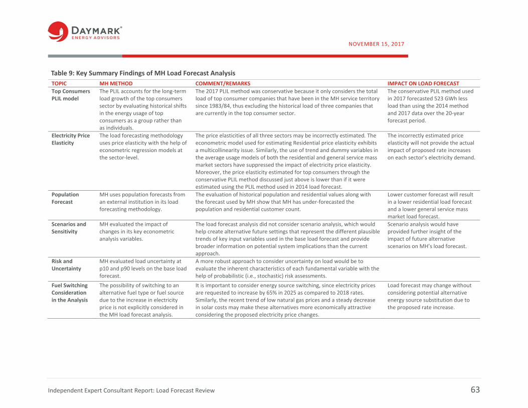
Table 9: Key Summary Findings of MH Load Forecast Analysis

TOPIC MH METHOD COMMENT/REMARKS IMPACT ON LOAD FORECAST

Top Consumers PLIL model

The PLIL accounts for the long‐term load growth of the top consumers sector by evaluating historical shifts in the energy usage of top consumers as a group rather than as individuals.

The 2017 PLIL method was conservative because it only considers the total load of top consumer companies that have been in the MH service territory since 1983/84, thus excluding the historical load of three companies that are currently in the top consumer sector.

The conservative PLIL method used in 2017 forecasted 523 GWh less load than using the 2014 method and 2017 data over the 20‐year forecast period.

Electricity Price Elasticity

The load forecasting methodology uses price elasticity with the help of econometric regression models at the sector‐level.

The price elasticities of all three sectors may be incorrectly estimated. The econometric model used for estimating Residential price elasticity exhibits a multicollinearity issue. Similarly, the use of trend and dummy variables in the average usage models of both the residential and general service mass market sectors have suppressed the impact of electricity price elasticity. Moreover, the price elasticity estimated for top consumers through the conservative PLIL method discussed just above is lower than if it were estimated using the PLIL method used in 2014 load forecast.

The incorrectly estimated price elasticity will not provide the actual impact of proposed rate increases on each sector’s electricity demand.

Population Forecast

MH uses population forecasts from an external institution in its load forecasting methodology.

The evaluation of historical population and residential values along with the forecast used by MH show that MH has under‐forecasted the population and residential customer count.

Lower customer forecast will result in a lower residential load forecast and a lower general service mass market load forecast.

Scenarios and Sensitivity

MH evaluated the impact of changes in its key econometric analysis variables.

The load forecast analysis did not consider scenario analysis, which would help create alternative future settings that represent the different plausible trends of key input variables used in the base load forecast and provide broader information on potential system implications than the current approach.

Scenario analysis would have provided further insight of the impact of future alternative scenarios on MH’s load forecast.

Risk and Uncertainty

MH evaluated load uncertainty at p10 and p90 levels on the base load forecast.

A more robust approach to consider uncertainty on load would be to evaluate the inherent characteristics of each fundamental variable with the help of probabilistic (i.e., stochastic) risk assessments.

Fuel Switching Consideration in the Analysis

The possibility of switching to an alternative fuel type or fuel source due to the increase in electricity price is not explicitly considered in the MH load forecast analysis.

It is important to consider energy source switching, since electricity prices are requested to increase by 65% in 2025 as compared to 2018 rates. Similarly, the recent trend of low natural gas prices and a steady decrease in solar costs may make these alternatives more economically attractive considering the proposed electricity price changes.

Load forecast may change without considering potential alternative energy source substitution due to the proposed rate increase.

NOVEMBER 15, 2017


Based on our analysis, Daymark has developed the following recommendations for

improving Manitoba Hydro’s current load forecasting methodology:

The load forecast analysis should consider scenario analysis by developing

alternative load forecasts in addition to the base load forecast. These scenarios

would help create alternative future settings that represent the different

possible trends of several key input variables that are used in generating the

base load forecast. Such scenarios could consider key uncertainties by

representing different assumptions for economic and population growth,

electricity and fuel commodity prices, and CO2 prices.

MH should evaluate the inherent characteristics of fundamental variables using

stochastic risk assessments. Currently, Manitoba Hydro’s method of evaluating

load uncertainty at p10 and p90 levels is based on considering the overall impact

of key input variables on the load variation. Using a stochastic risk assessment

method would allow for the estimating of potential outcomes by allowing

random variation in key input variables. Probabilities are assigned to different

values of key uncertain variables which have optimally been identified through

sensitivity analysis.

MH may generate a better estimate of weather‐dependent load by using more

than two years of monthly energy and degree day data to estimate the weather‐

dependent relationship. Currently, the company uses two years of data to

estimate the weather‐dependent load relationship and 25 years of data to

define the “normal” weather year. Also, Manitoba Hydro could improve its

weather normalization method by using a shorter period to calculate the

“normal” year weather variables.

MH should consider testing its econometric models of different statistical issues.

For example, the average usage regression models contain multicollinearity

issues. Similarly, MH should consider the economic reasoning before introducing

any new predictor variables in its regression models in addition to checking the

statistical significance.

Daymark also compared the 2014 and 2017 load forecast methodologies and

assumptions for the various customer groups defined by Manitoba Hydro. Overall, the

2017 methods generated a lower long‐term forecast than the analysis conducted in 2014

with the 10‐year historical growth rate of gross frim energy forecasted in 2017 being

NOVEMBER 15, 2017


lower than the 2014 forecasted gross firm energy. Additionally, the annual growth rate

using ten‐year gross firm energy forecast was higher in 2014 at 1.46% compared to

0.81% in the 2017 forecast. The key differences between 2014 and 2017 load forecast

methodologies are in the models used for forecasting mass market customer (GSMM)

count, PLIL method used for capturing long‐term forecast for top consumer category,

and economic and population assumptions used in the analysis.

In order to estimate the customer count for GSMM category, the 2017 forecast

estimated customer count directly while the 2014 forecast modeled the percentage

change in the number of customer types. The 2017 PLIL method used a conservative

approach by only considering the total load of top consumer companies that have been

in MH’s service territory since 1983/84, the start year of MH’s modeling period.

Whereas, 2014 PLIL methodology considered load of all companies included in the top

consumer category.

B‐66 Independent Expert Consultant Report: Load Forecast Review

APPENDIX A


Scope of Work

DAYMARK ENERGY ADVISORS

Scope of Work

Export Pricing and Revenues Review

1. Review Manitoba Hydro's electricity export price forecast and third party consultant

forecasts, including the low and high case forecasts, in the context of current MISO

market conditions and factors influencing future MISO prices. The third party consultant

forecasts are to be taken as a "given" and are to be assumed to be reasonable and

accurate with respect to the other tasks in this Scope of Work. Notwithstanding that the

third party consultant forecasts are to be accepted for the purposes of this review, if the

IEC identifies significant issues or inconsistencies with the third party consultant

forecasts in the course of its general review, those issues or inconsistencies are to be,

identified in the IEC's reports.

2. Review and assess Manitoba Hydro's forecast of exportable surplus energy and

capacity by on-peak and off-peak period, taking into account expected inflow conditions,

reservoir levels, and tie line capacities.

3. Review Manitoba Hydro's forecast for export revenues and fuel & power purchases for

the next twenty years and assess whether the forecast of net extraprovincial revenue is

reasonable. As an independent review of the extraprovincial revenues arising from

contracted energy and capacity sales was undertaken at the 2014 NFAT (Exhibit LCA-5

in response to CSI Undertaking UT-34), a review of Manitoba Hydro's export contracts

and estimation by the IEC of firm energy revenues and capacity revenues is not required

for any contracts that were contemplated and assessed at the NFAT. Manitoba Hydro's

updated export revenues, volumes, and unit prices by contract and by year will be

provided as part of PUB MFR-84. The firm energy and capacity revenues in PUB MFR-

84, for those contracts evaluated by the IEC at the NFAT, are to be taken as "given", so

long as the firm energy and capacity revenues are aligned with the independent analysis

from the NFAT after adjusting for changes in forecast exchange rates and escalation.

4. Assess the reasonableness of changes in Manitoba Hydro's forecasting methodology

that eliminates the assumed premiums for surplus dependable energy and capacity

sales.

5. Provide comments on the factors influencing the MISO market and trends that are

affecting market prices, including but not limited to:

(a) state and federal policies on electricity generation and emissions;

(b) existing generation mix;

(c) expected new generation to be installed in the next 20 years;

(d) forecasted generation retirements in the next 20 years;

(e) supply and demand balance in the northern MISO region; and

(1) factors that may affect Manitoba Hydro's ability to export energy and

capacity into the MISO market.

6. Provide a report to be placed on the public record that provides the, Cense!tent's

findings, opinions, and non-commercially sensitive supporting information.

7. Provide a non-public report to the PUB that provides commercially sensitive information

and additional calculations supporting the findings.

Public and Commercially Sensitive Load Forecast Review

8. Review Manitoba Hydro's 2017 Load Forecast and assess the changes with respect to

the 2014 Load Forecast.

9. Assess Manitoba Hydro's load forecasting methods for Residential, Mass Market, and

Top Consumers segments and compare to industry best practices with respect to:

(a) the econometric and end-use forecasting methodology;

(b) the elasticity methodology used to evaluate how Manitoba Hydro evaluates

the implications of rate increases and new technology on electricity demand.

(c) Manitoba Hydro's economic assumptions including population growth, GDP

growth, and price elasticity;

(d) the reliability of the short and long-term domestic load forecast modelling;

(e) the extent to which Manitoba Hydro has used appropriate scenario planning

to examine the potential impact of changes in the industry, the Manitoba and

Canadian economies, available technology (generation and loads) and

energy efficiency measures (costs and cost effectiveness);

(f) the appropriate use of probability analysis of projected load forecasts;

(g) the extent to which retrospective load analysis provides confidence in the

load forecast;

(h) the reasonableness of peak demand and energy trends including seasonal

variations in load forecasting; and

(i) impacts on load forecasts resulting from potential fuel switching, particularly

in light of recent trends in the cost of natural gas and potential carbon taxes.

10. Assess other aspects of the load forecasting methodology including transmission and

distribution losses.

11. Evaluate the historical performance of Manitoba Hydro's load forecasting methodologies

for Residential, Mass Market, and Top Consumers segments.

12. Review the commercially sensitive load forecast for Top Consumers and assess the

reasonableness of the forecasting methods and forecast.

13. Coordinate with other 1ECs who are reviewing price elasticity impacts on electricity

demand in order to minimize duplication of analysis.

14. Provide a report to be placed on the public record that provides the Consultant's

findings, opinions, and non-commercially sensitive supporting information.

15. Provide a non-public report to the PUB that provides commercially sensitive information

and additional calculations supporting the findings.

APPENDIX B


Documents Relied Upon

Independent Expert Consultant Report: Load Forecast Review B‐1

Consistent with the agreement between Daymark Energy Advisors and the Manitoba

Public Utilities Board, the following appendix provides a reference to the documents

that were relied upon to develop this Independent Expert Consultant Report.

This appendix is organized into two sections. The first is a list of the documents relied

upon that are already part of the record in this docket. The second is an annotated

bibliography of additional documents relied upon that are not already part of the record

in this docket.

Documents in the Record

Document Name: Confidential or Non-Confidential:

Manitoba Hydro, "2017 Electric Load Forecast", Market Forecast June 2017.

Non‐Confidential

NOVEMBER 15, 2017


Annotated Bibliography of Additional Documents

Document or File Name: Confidential or

Non-Confidential:

Publicly‐Sourced Documents

BC Hydro Power Smart, “Fiscal 2017 to Fiscal 2019 Revenue Requirements Application”, ERRATA, August 17, 2016.

Non‐Confidential

Ernest Orlando Lawrence Berkeley National Laboratory “Load Forecasting in Electric Utility Integrated Resource Planning”, October 2016.

Non‐Confidential

Cameron, “Making Regression Analysis More Useful, II: Dummies and Trends”, Chapter 7.

Non‐Confidential

Itron, “PGE Forecast Review Summary”, April 2015. Non‐Confidential

Itron, “2013 Forecasting Benchmarking Study”, August 29, 2013. Non‐Confidential

Wilkerson, Jordan, et al., “Survey of Western U.S. electric utility resource plans”, December 13, 2013.

Non‐Confidential

Public Documents from Manitoba Hydro

Manitoba Hydro, "2016 Electric Load Forecast", Market Forecast June 2016. Non‐Confidential

Manitoba Hydro, "2011 Electric Load Forecast (For External Use)", Market Forecast May 2011, Approved July 2011, Revised May 2012.

Non‐Confidential

Confidential Document from Manitoba Hydro

BMO Capital Markets, “Provincial Monitor”, Spring 2017 Confidential

IFF16 Update with Interim Projected Retail Rates Confidential

“Error Eval – Manitoba Pop 2016.xlsx” Confidential

CAC/CENTRA I‐10a Confidential

CAC/CENTRA I‐13 Confidential

Christian Associates Energy Consulting, “Review of Forecast Methods Underlying the 2015 Energy Forecast for Manitoba Hydro”, October 6, 2015.

Confidential

Navius Research Inc., “Review of Forecasting Methods Used by Manitoba Hydro’s Economic Analysis Department (EAD)”, February 28, 2014.

Confidential

“Elec Heat Market Share 2017_Daymark.xlsx” Confidential

NOVEMBER 15, 2017

Independent Expert Consultant Report: Load Forecast Review B‐3


Non-Confidential:

Manitoba Hydro, "2014 Electric Load Forecast (For Internal Use Only)", Market Forecast, August 2014.

Confidential

Manitoba Hydro, "2015 Electric Load Forecast (For Internal Use Only)", Market Forecast June 2015.

Confidential

“Electric Vehicles 2017_Daymark.xlsx” Confidential

“Error Evaluation – Interest Rates 2015.xlsx” Confidential

“Error Evaluation – Manitoba Population 2016.xlsx” Confidential

“Gen2017‐Daymark.xlsx” Confidential

“GeneralConsumersAndManitobaFirm.xlsx” Confidential

Manitoba Hydro, “GS Average Use Model, The AUTOREG Procedure”. Confidential

“GS Large Cust 2017.xlsx” Confidential

“GS Mass Market 2017 – May 1st_Daymark.xlsx” Confidential

Manitoba Hydro, “GS Small and Medium Cust Model, The AUTOREG Procedure”. Confidential

“GSTop_10_2017_Daymark.xlsx” Confidential

“GSTop_2014_Daymark.xlsx” Confidential



Manitoba Hydro, “Manitoba Hydro Weather Normalization, Model Sharing Session, Itron Annual Energy Forecasting Meeting.”

Confidential

“Load Forecast Data – Formulas.xlsx” Confidential

“MB RGDP exercise.xlsx” Confidential

“MHResCustForecast.xlsx” Confidential

Manitoba Hydro, “Top Consumers PLIL Model, The AUTOREG Procedure”. Confidential

“PopulationForecast2017.xlsx” Confidential

PUB MFR 97‐Top Consumers LF 2017 – CONFIDENTIAL Confidential

Manitoba Hydro, “Res Average Use Model, The AUTOREG Procedure.” Confidential

NOVEMBER 15, 2017



Non-Confidential:

“Res AveUse Model 2017_Daymark.xlsx” Confidential

“Res End Use 2017_electric_final_Daymark.xlsx” Confidential

“SurveyOfForecasters2017.xlsx” Confidential

“Top Consumer PLIL 2017_Daymark.xlsx” Confidential

“WeatherNormalization‐Daymark.xlsx” Confidential

“WeatherNormalizationUpdated2‐Daymark.xlsx” Confidential

“WeatherNormalizationUpeated‐Daymark.xlsx” Confidential

Date post:	18-Apr-2020
Category:	Documents
Upload:	others
View:	13 times
Download:	0 times