93
| Date post: | 07-Jul-2018 |
| Category: |
Documents |
| Upload: | duongthien |
| View: | 215 times |
| Download: | 0 times |

1

TABLE OF CONTENTS
CHAPTER PAGE
1 OVERVIEW : : : : : : : : : : : : : : : : : : : : : : : : : : : : : : : : : : : 5
1.1 Capabilities of Robotica : : : : : : : : : : : : : : : : : : : : : : : : : : 5
1.2 Requirements : : : : : : : : : : : : : : : : : : : : : : : : : : : : : : : : 6
2 BASIC CONCEPTS : : : : : : : : : : : : : : : : : : : : : : : : : : : : : : 7
2.1 Loading Robotica : : : : : : : : : : : : : : : : : : : : : : : : : : : : : : 7
2.2 Lists in Mathematica : : : : : : : : : : : : : : : : : : : : : : : : : : : 7
2.3 Input File Format : : : : : : : : : : : : : : : : : : : : : : : : : : : : : 8
2.4 Robotica Notation : : : : : : : : : : : : : : : : : : : : : : : : : : : : : : 11
2.5 The Help Command : : : : : : : : : : : : : : : : : : : : : : : : : : : : 11
3 FORWARD KINEMATICS : : : : : : : : : : : : : : : : : : : : : : : : : : 13
3.1 Loading a Robot : : : : : : : : : : : : : : : : : : : : : : : : : : : : : : 13
3.2 Generating the Equations : : : : : : : : : : : : : : : : : : : : : : : : 14
3.3 Printing Results : : : : : : : : : : : : : : : : : : : : : : : : : : : : : : 15
3.4 Summary : : : : : : : : : : : : : : : : : : : : : : : : : : : : : : : : : : : 18
4 ARM GRAPHICS : : : : : : : : : : : : : : : : : : : : : : : : : : : : : : : : 19
4.1 Arm Construction : : : : : : : : : : : : : : : : : : : : : : : : : : : : : 21
4.2 Design Guidelines for Joints : : : : : : : : : : : : : : : : : : : : : : : 22
4.3 An Example : : : : : : : : : : : : : : : : : : : : : : : : : : : : : : : : : 23
4.4 Planar Arm Interjoint Shapes : : : : : : : : : : : : : : : : : : : : : : 24
4.5 Animation and other Options : : : : : : : : : : : : : : : : : : : : : : 27
5 DYNAMICS : : : : : : : : : : : : : : : : : : : : : : : : : : : : : : : : : : : 28
5.1 Loading a Robot : : : : : : : : : : : : : : : : : : : : : : : : : : : : : : 28
2

5.2 Generating the Equations : : : : : : : : : : : : : : : : : : : : : : : : 29
5.3 Printing Results : : : : : : : : : : : : : : : : : : : : : : : : : : : : : : 30
5.4 Summary : : : : : : : : : : : : : : : : : : : : : : : : : : : : : : : : : : : 31
6 DYNAMICS RESPONSE COMPUTATION : : : : : : : : : : : : : : : 35
6.1 De�ning the Torque Vector : : : : : : : : : : : : : : : : : : : : : : : 35
6.2 Calling Response : : : : : : : : : : : : : : : : : : : : : : : : : : : : : : 36
6.3 Saving Results : : : : : : : : : : : : : : : : : : : : : : : : : : : : : : : 37
6.4 Viewing Results : : : : : : : : : : : : : : : : : : : : : : : : : : : : : : 38
6.5 Two-Link Example : : : : : : : : : : : : : : : : : : : : : : : : : : : : : 39
7 MANIPULABILITY : : : : : : : : : : : : : : : : : : : : : : : : : : : : : : 44
7.1 Generating the Ellipsoids : : : : : : : : : : : : : : : : : : : : : : : : 44
7.2 Options : : : : : : : : : : : : : : : : : : : : : : : : : : : : : : : : : : : : 45
7.3 Examples : : : : : : : : : : : : : : : : : : : : : : : : : : : : : : : : : : : 47
8 EXTERNAL SIMULATION COMPATIBILITY : : : : : : : : : : : : : 52
8.1 Loading Simulation Data : : : : : : : : : : : : : : : : : : : : : : : : : 52
8.2 Simulation Input File Format : : : : : : : : : : : : : : : : : : : : : : 54
8.3 Plotting Simulation Data : : : : : : : : : : : : : : : : : : : : : : : : : 54
8.4 Examples : : : : : : : : : : : : : : : : : : : : : : : : : : : : : : : : : : : 55
9 ROBOTICA FRONT END : : : : : : : : : : : : : : : : : : : : : : : : : : 60
9.1 The Structure of RFE : : : : : : : : : : : : : : : : : : : : : : : : : : : 60
9.2 Menu Bar : : : : : : : : : : : : : : : : : : : : : : : : : : : : : : : : : : 60
9.2.1 File : : : : : : : : : : : : : : : : : : : : : : : : : : : : : : : : : : 60
9.2.2 Packages : : : : : : : : : : : : : : : : : : : : : : : : : : : : : : : 61
9.3 Mathematica Output Window : : : : : : : : : : : : : : : : : : : : : 62
9.4 Command Input Line : : : : : : : : : : : : : : : : : : : : : : : : : : : 63
9.5 Robotica Function Selection Menu : : : : : : : : : : : : : : : : : : : : 63
10 COMMAND REFERENCE : : : : : : : : : : : : : : : : : : : : : : : : : : 66
APrint : : : : : : : : : : : : : : : : : : : : : : : : : : : : : : : : : : : : : : : : 66
3

ClearLinkShape : : : : : : : : : : : : : : : : : : : : : : : : : : : : : : : : : : : 66
ClearPrisJoint : : : : : : : : : : : : : : : : : : : : : : : : : : : : : : : : : : : : 67
ClearRevJoint : : : : : : : : : : : : : : : : : : : : : : : : : : : : : : : : : : : : 67
CPrint : : : : : : : : : : : : : : : : : : : : : : : : : : : : : : : : : : : : : : : : 67
DataFile : : : : : : : : : : : : : : : : : : : : : : : : : : : : : : : : : : : : : : : 68
ELDynamics : : : : : : : : : : : : : : : : : : : : : : : : : : : : : : : : : : : : 68
EPrint : : : : : : : : : : : : : : : : : : : : : : : : : : : : : : : : : : : : : : : : 68
FKin : : : : : : : : : : : : : : : : : : : : : : : : : : : : : : : : : : : : : : : : : 69
GetInputTau : : : : : : : : : : : : : : : : : : : : : : : : : : : : : : : : : : : : 69
LoadAnim : : : : : : : : : : : : : : : : : : : : : : : : : : : : : : : : : : : : : : 69
LinkShape : : : : : : : : : : : : : : : : : : : : : : : : : : : : : : : : : : : : : : 69
MPrint : : : : : : : : : : : : : : : : : : : : : : : : : : : : : : : : : : : : : : : : 70
Planar : : : : : : : : : : : : : : : : : : : : : : : : : : : : : : : : : : : : : : : : 70
PrintInputData : : : : : : : : : : : : : : : : : : : : : : : : : : : : : : : : : : : 71
PrisJoint : : : : : : : : : : : : : : : : : : : : : : : : : : : : : : : : : : : : : : : 71
RElp : : : : : : : : : : : : : : : : : : : : : : : : : : : : : : : : : : : : : : : : : 71
Response : : : : : : : : : : : : : : : : : : : : : : : : : : : : : : : : : : : : : : 74
RevJoint : : : : : : : : : : : : : : : : : : : : : : : : : : : : : : : : : : : : : : : 74
SDynamics : : : : : : : : : : : : : : : : : : : : : : : : : : : : : : : : : : : : : 75
SaveAnim : : : : : : : : : : : : : : : : : : : : : : : : : : : : : : : : : : : : : : 75
SaveResponse : : : : : : : : : : : : : : : : : : : : : : : : : : : : : : : : : : : : 75
SeqShowRobot : : : : : : : : : : : : : : : : : : : : : : : : : : : : : : : : : : : 76
SetRanges : : : : : : : : : : : : : : : : : : : : : : : : : : : : : : : : : : : : : : 78
ShowAnim : : : : : : : : : : : : : : : : : : : : : : : : : : : : : : : : : : : : : : 78
ShowRobot : : : : : : : : : : : : : : : : : : : : : : : : : : : : : : : : : : : : : 78
SimDrive : : : : : : : : : : : : : : : : : : : : : : : : : : : : : : : : : : : : : : 80
SimplifyExpression : : : : : : : : : : : : : : : : : : : : : : : : : : : : : : : : : 82
SimplifyTrigNotation : : : : : : : : : : : : : : : : : : : : : : : : : : : : : : : : 82
SimPlot : : : : : : : : : : : : : : : : : : : : : : : : : : : : : : : : : : : : : : : 82
TPrint : : : : : : : : : : : : : : : : : : : : : : : : : : : : : : : : : : : : : : : : 83
4

A KINEMATICS AND DYNAMICS EQUATIONS : : : : : : : : : : : : 85
REFERENCES : : : : : : : : : : : : : : : : : : : : : : : : : : : : : : : : : 89
5

LIST OF TABLES
Table Page
2.1 Robotica notation. : : : : : : : : : : : : : : : : : : : : : : : : : : : : : : : 12
6

LIST OF FIGURES
Figure Page
2.1 The c.o.m. vectors for a two-link arm. : : : : : : : : : : : : : : : : : : : 11
3.1 Successful read operation. : : : : : : : : : : : : : : : : : : : : : : : : : : 14
3.2 Results of FKin[] on input data. : : : : : : : : : : : : : : : : : : : : : : : 15
3.3 MPrint[] usage. : : : : : : : : : : : : : : : : : : : : : : : : : : : : : : : : 15
3.4 Results of SimplifyTrigNotation[]. : : : : : : : : : : : : : : : : : : : : : : 16
3.5 The Jacobian for the two degree of freedom robot. : : : : : : : : : : : : : 16
3.6 Output from EPrint[]. : : : : : : : : : : : : : : : : : : : : : : : : : : : : 17
4.1 Standard revolute joint. : : : : : : : : : : : : : : : : : : : : : : : : : : : 19
4.2 Standard prismatic joint. : : : : : : : : : : : : : : : : : : : : : : : : : : : 20
4.3 Stanford arm. : : : : : : : : : : : : : : : : : : : : : : : : : : : : : : : : : 20
4.4 New prismatic joint. : : : : : : : : : : : : : : : : : : : : : : : : : : : : : 24
4.5 Stanford arm with new joint shapes. : : : : : : : : : : : : : : : : : : : : 25
4.6 Arm with standard shapes. : : : : : : : : : : : : : : : : : : : : : : : : : : 26
4.7 Arm with new link shape. : : : : : : : : : : : : : : : : : : : : : : : : : : 26
5.1 Successful read operation. : : : : : : : : : : : : : : : : : : : : : : : : : : 29
5.2 Results of ELDynamics[]. : : : : : : : : : : : : : : : : : : : : : : : : : : : 30
5.3 The elements of the mass matrix. : : : : : : : : : : : : : : : : : : : : : : 31
5.4 Results of running Simplify TrigNotation[]. : : : : : : : : : : : : : : : : : 32
5.5 Examining the Christo�el symbols. : : : : : : : : : : : : : : : : : : : : : 33
5.6 The Jvc matrices. : : : : : : : : : : : : : : : : : : : : : : : : : : : : : : : 33
5.7 G, the gravity vector. : : : : : : : : : : : : : : : : : : : : : : : : : : : : : 34
6.1 Reading the input torque vector. : : : : : : : : : : : : : : : : : : : : : : 36
6.2 Joint parameter q1 tracking a Sine wave. : : : : : : : : : : : : : : : : : : 39
7

6.3 Circular motion control de�nitions. : : : : : : : : : : : : : : : : : : : : : 41
6.4 Joint variables as a function of time. : : : : : : : : : : : : : : : : : : : : 42
6.5 Arm location from circular controller. : : : : : : : : : : : : : : : : : : : : 42
6.6 End e�ector location from circular controller. : : : : : : : : : : : : : : : : 43
7.1 Planar manipulability example. : : : : : : : : : : : : : : : : : : : : : : : 48
7.2 Scaling the ellipsoids. : : : : : : : : : : : : : : : : : : : : : : : : : : : : : 49
7.3 Three-link example. : : : : : : : : : : : : : : : : : : : : : : : : : : : : : : 50
7.4 Three-link nonplanar example. : : : : : : : : : : : : : : : : : : : : : : : : 50
7.5 A change of ViewPoint. : : : : : : : : : : : : : : : : : : : : : : : : : : : : 51
8.1 Loading a SIMNON �le. : : : : : : : : : : : : : : : : : : : : : : : : : : : 55
8.2 Two link planar arm driven with dataset. : : : : : : : : : : : : : : : : : : 56
8.3 Plot of the end e�ector location. : : : : : : : : : : : : : : : : : : : : : : : 57
8.4 Time, t, versus q1 and q2. : : : : : : : : : : : : : : : : : : : : : : : : : : 58
8.5 Joint parameter q1 versus q2. : : : : : : : : : : : : : : : : : : : : : : : : 59
9.1 Robotica Front End. : : : : : : : : : : : : : : : : : : : : : : : : : : : : : : 61
9.2 Output in the Mathematica output window. : : : : : : : : : : : : : : : : 62
9.3 DataFile option screen. : : : : : : : : : : : : : : : : : : : : : : : : : : : : 64
9.4 SimDrive option screen. : : : : : : : : : : : : : : : : : : : : : : : : : : : 64
A.1 Denavit-Hartenburg frame assignment [3]. : : : : : : : : : : : : : : : : : 85
8

CHAPTER 1
OVERVIEW
1.1 Capabilities of Robotica
Robotica1 is a collection of useful robotics problem solving functions encapsulated in
a Mathematica package. Utilizing Mathematica's computational features allows results
to be generated in a purely symbolic form. The bene�t of the symbolic representation is
that the problem is solved for all possible input parameter values at once, and the user
can then substitute and experiment with actual numbers to discover the e�ects of various
parameters.
Robotica requires input in the form of a table of Denavit-Hartenberg parameters
describing the robot to be analyzed. Once the table has been entered, Robotica can
generate the forward kinematics for the robot. The A and T matrices as well as the
velocity Jacobian, J , are generated. Of course, it is possible to display and save to an
external �le all of the data generated. If the dynamics equations of the robot are also
to be generated, the input must include the dynamics description data as detailed in
Chapter 2.
Once the forward kinematics are produced, Euler-Lagrange dynamics equations can
be calculated. The inertia matrix, Coriolis and centrifugal terms, Christo�el symbols
and gravity vectors are all available to the user once the dynamics routines have run.
Utilizing the forward kinematics results, Robotica can calculate the manipulability
ellipsoids when supplied with a range of joint variable values. It is possible to generate
and save a list of manipulability measures as well as display the ellipsoids with the robot
on the screen.
1Robotica
TM is a trademark of The Board of Trustees of the University of Illinois.
9

In addition, Robotica has the capability of reading external simulation (e.g., SIM-
NON [1]) output �les and displaying the motion of the robot when subjected to the
sequence of joint variable changes described in the �le. This requires that the robot has
been input as a table of Denavit-Hartenburg parameters, and that the forward kinematics
routines have been executed.
Robotica contains several functions that can be used to draw the robot in a spe-
ci�c con�guration, or show the robot moving through a range of joint parameter val-
ues. Most of the graphics output can be animated if the Animation.m package is
loaded, this includes the graphics produced with SimDrive[], RElp[], ShowRobot[], and
SeqShowRobot[]. The animations can be saved and later restored and viewed again. See
the functions SaveAnim[], LoadAnim[], ShowAnim[], and SetRanges[] in Appendix A for
more details.
To simplify interaction with Robotica, an X-Windows based interface has been de-
signed. The interface insulates the user from the inconvenient textual interface Mathe-
matica provides (see Chapter 9 for details.)
1.2 Requirements
Running Robotica directly through Mathematica requires Mathematica release 2.0 or
better, while running Robotica through the X-Windows front end requires Mathematica
2.1 or better. Much of Robotica deals with text only input and output; however, there are
functions which produce graphical output which requires a machine capable of producing
the displays.
10

CHAPTER 2
BASIC CONCEPTS
2.1 Loading Robotica
Once Mathematica has been started (check that the version is 2.0 or greater), the
Robotica package can be loaded with the following command:
In[1] := << robotica.m
At this point, all of the functions provided by the package are available to the user
(although some may require that other actions have been performed �rst, e.g., running
FKin[] before ELDynamics[]). Mathematica is case sensitive, thus it is important to type
the function names exactly as they appear in the text, e.g., FKin[] is entered as capital
F, capital K, lower case i, lower case n, open [, close ].
2.2 Lists in Mathematica
There are several functions in Robotica that take lists as input parameters. There
are a few basic rules governing lists that should be understood when specifying them to
functions.
First, a list begins with an opening f, ends with a closing g, and contains elements
separated by commas (if there is more than one). For example, ftraceg is a list containing
one element called trace and ftrace, printg is a list containing the two elements trace,
and print.
In addition, Lists can include just about anything as elements: symbols, numbers,
even other lists. For example, ffq1; 0; 3:1415g; 6g, is a list containing another list,
11

fq1; 0; 3:1415g, and the number 6. This inner list contains three elements, q1, 0, and
3.1415.
If there is a list that is used frequently, it is sometimes more convenient to assign
some variable name to it than to retype it every time it is used. For example:
In[5] := simlist = fd1, q2g
In[6] := SimPlot[t, simlist]
Whenever Mathematica sees simlist, it will substitute the list fd1, q2g, which can save
much unnecessary user input. See [2] for more information about lists, and Mathematica
in general.
2.3 Input File Format
A convenient way to specify input data to Robotica is through a data �le. Denavit-
Hartenberg parameters and dynamics data for the robot can be given in such a �le. A
representative input data �le is shown below (there are line numbers at the beginning of
each line which are for reference only | they should not actually be present in a data�le:
[01] A Robotica input data �le for
[02] a two degree of freedom planar robot
[03] ||||||||||{
[04] DOF = 2
[05] The Denavit-Hartenberg parameters:
[06] joint1 = revolute
[07] a1 = a1
[08] alpha1 = 0
[09] d1 = 0
[10] theta1 = q1
[11] joint2 = revolute
[12] a2 = a2
[13] alpha2 = 0
[14] d2 = 0
12

[15] theta2 = q2
[16]
[17] The dynamics information:
[18]
[19] DYNAMICS
[20]
[21] gravity vector = f0,g,0g
[22] mass1 = m1
[23] center of mass = f-(1/2) a1, 0,0g
[24] inertia matrix = f0,0,0,0,0,I1g
[25] mass2 = m2
[26] center of mass = f-(1/2) a2, 0, 0g
[27] inertia matrix = f0,0,0,0,0,I2g
In this example, lines [01] through [03] are a general comment, and are ignored. In
general, there can be any number of such comment lines prefacing the data.
Line [04] tells Robotica that Denavit-Hartenberg parameters are coming. The keyword
DOF is used by Robotica to decide when to start reading the parameters; DOF should
be followed by an equals sign (`=') then the number of links in the robot.
Line [05] is provided as a comment line, it is skipped over when reading the data. If
no comment is wanted, leave this line blank.
Lines [06] through [10] contain the Denavit-Hartenberg parameters for the �rst link.
The line joint1 = revolute tells Robotica that the �rst link is a revolute type. Two types
of links are supported by Robotica: revolute and prismatic (sliding). If the link had been
prismatic, line [06] would have read joint1 = prismatic. Line [07] speci�es the a parameter
for the link, line [08] gives the alpha parameter, line [09] supplies the d parameter, and
line [10] speci�es the theta variable. The parameters must be given in that order: a,
alpha, d, and theta. The format for each line is: label = parameter. The label is ignored,
and the parameter is assigned to its respective Denavit-Hartenberg parameter for that
link. There must be exactly one space or tab after the equals sign.
13

Lines [11] through [15] give the corresponding data for link two. The comments in the
above paragraph apply. There should be no space between consecutive data segments
for neighboring links.
Lines [16] through [18] are a general comment, and are ignored by Robotica. In general,
there can be any number of such comment lines as a preface to the dynamics data.
Line [19] contains the required keyword DYNAMICS to indicate to Robotica that
dynamics input data are to follow.
Line [20] is provided as a comment line, it is skipped over when reading the data. If
no comment is wanted, leave this line blank.
Line [21] gives the gravity vector in standard x,y,z form. This vector is understood
by Robotica to be referenced to the base frame.
Lines [22] through [24] give the dynamics data for the �rst link. In line [22], mass1
= m1 assigns the variable m1 to be the mass of the �rst link. Line [23] supplies the
location of the center of mass for link one in terms of the coordinate frame for link one.
The format is a list of x, y, and z o�sets. In Mathematica, a list is surrounded by braces,
thus the input here is -(1/2) a1, 0,0 which means that the center of mass for this link is
back (1/2) of the length of this link in the x-direction, 0 in the y-direction, and 0 in the
z-direction (in terms of the coordinate frame for link one). Figure 2.1 shows the c.o.m.
setup for a two-link arm.
Line [24] gives the six unique components of the symmetric inertia tensor, in list
format. These are assigned as follows:
fe1; e2; e3; e4; e5; e6g ==>
����������
e1 e2 e3
e2 e4 e5
e3 e5 e6
����������The inertia tensor for link i is a 3� 3 matrix computed in the coordinate frame attached
to link i. See Equation [6.2.19] in [3] for complete information. The format for each
line is: label = parameter. The label is ignored, and the parameter is assigned to its
respective Denavit-Hartenberg parameter for that link.
Lines [25] through [27] give the dynamics information for the next link. The comments
of the above paragraphs apply to these lines.
14

Y2
X2
Z2
x
x
x
.��
��
6
�
-
6
������������
@@@I
?
X
Y
Z
0
0 0
X1Y1
Z1link1
link2
com = f -(1/2)a2, 0, 0g
com = f - (1/2)a1, 0, 0g
Figure 2.1: The c.o.m. vectors for a two-link arm.
Of course, if the generation of forward kinematics equations are all that Robotica will
be used for, the dynamics portion of the �le need not exist. Note also that for each
degree of freedom (speci�ed by DOF = n) there must be a set of Denavit-Hartenberg
parameters, and if dynamics data are given, there must also be a set of data for each
degree of freedom.
2.4 Robotica Notation
The notation that Robotica uses to store the various quantities and parameters is
summarized in Table 2.1. In general, the names Robotica uses are as close as possible to
standard mathematical notation. To access the variable in Robotica, one merely types
the correct Robotica notation at the prompt.
2.5 The Help Command
Mathematica provides a built-in help command, ?. It may be used to request infor-
mation about any Mathematica command or function as well as all Robotica functions
15

available to the user. For example, to obtain information about the RElp[] function, type:
? RElp[], and Mathematica will respond with a brief help message about the function.
Table 2.1: Robotica notation.
NotationCorrespondingRoboticaNotation
NotationCorrespondingRoboticaNotation
ai a[i] gi gravity[i]di d[i] mi mass[i]�i alpha[i] comi com[i]�i theta[i] Ii inertia[i]Ai A[i] Jci Jc[i]T kj T[j,k] Jvci Jvc[i]J J Jwci Jwc[i]Ji Jvw[i] cijk c[[i,j,k]]zi z[i] Cos(q1) C1oi o[i] Sin(q1) S1M M Cos(q1 + q2) C12C CM Sin(q1 + q2) S12g G Cos(q1 � q2) C1-2
Sin(q1 � q2) S1-2Cos(q1 + q2 + q3) C123Sin(q1 + q2 + q3) S123Cos(q1 + q2 � q3) C12-3Sin(q1 + q2 � q3) S12-3
16

CHAPTER 3
FORWARD KINEMATICS
One of the primary features of Robotica is its ability to generate the forward kinemat-
ics equations for any robot described by Denavit-Hartenberg parameters. The mathe-
matics behind this process is described in Appendix B. Essentially, Robotica will compute
the A matrices, T matrices, and Jacobian (see [3]) for the arm.
3.1 Loading a Robot
The �rst step in the process of generating the equations is to load the data �le. The
Robotica command \DataFile[]" is used for this purpose; it can be used in two ways:
DataFile[\�lename"] or DataFile[].
The �rst method speci�es the �lename from which to load the data; it must be a
quoted string. For example, DataFile[\twodof"] loads the �le \twodof" if it exists in the
�le system. Entering DataFile[] without the �lename parameter will cause Robotica to
prompt for the �lename. Simply type the �lename without quotes in response to the
query and Robotica will load the �le. The following lines show the two possibilities:
In[2] := DataFile[\twodof"]
or
In[2] := DataFile[]
Enter Data File Name : twodof
If the data �le is in the correct format, and DataFile[] successfully reads the parameters,
a table will be displayed showing what Robotica has stored internally from the �le. If the
�le does not exist, or is incorrectly formatted, a message will be displayed to that e�ect,
17

and Robotica will not store anything. Figure 3.1 shows what a successful read operation
looks like.
0
0
0
0
0
0
0
0
I1
0
0
0
0
0
0
0
0
I2
Link
1
2
mass
m1
m2
com vector
[-a1/2, 0, 0]
[-a2/2, 0, 0]
Inertia[1]=
Inertia[2]=
In[2]:= Data�le[]
Enter data �le name: newtwo
State Reset...
Kinematics Input Data|||||Joint
1
2
Type
revolute
revolute
a
a1
a2
alpha
0
0
d
0
0
theta
q1
Dynamics Input Data||||{
q2
Gravity vector: [0,g,0]
Figure 3.1: Successful read operation.
3.2 Generating the Equations
Once the data �le has been loaded, it is very simple to generate the forward kinematics
equations; the command FKin[] is used for this purpose. FKin[] takes no parameters,
and displays a report of the various quantities computed. Figure 3.2 shows a sample run
of FKin[] on the data �le of Figure 3.1.
18

In[4]:=FKin[]
A Matrices Formed:
A[1]
A[2]
T Matrices Formed:
T[0,0]
T[0,1]
T[0,2]
T[1,2]
Jacobian Formed
Jacobian (6x2)
Figure 3.2: Results of FKin[] on input data.
3.3 Printing Results
After the forward kinematics equations have been generated, showing the results is
accomplished through a set of display functions provided within Robotica. MPrint[] is
such a function; it takes up to three parameters: the matrix to be displayed (required),
a text label to print alongside the matrix (required), and a �lename in quotes in which
to save the matrix (optional). Figure 3.3 shows how MPrint[] is used to display the
matrix A[2].
Out[5]=
A2=
Cos[q2]
Sin[q2]
0
0
-Sin[q2]
Cos[q2]
0
0
0
0
1
0
a2 Cos[q2]
a2 Sin[q2]
0
1
In[5]:= MPrint[A[2], \A2="]
Figure 3.3: MPrint[] usage.
19

It is sometimes convenient to change the trigonometric notation to be somewhat
more succinct. The function SimplifyTrigNotation[] takes no parameters, and modi�es
the display of Sin[] and Cos[] to an abbreviated form. Figure 3.4 shows the results of
running SimplifyTrigNotation[].
In[5]:= SimplifyTrigNotation[]
Out[7]=
A2=
C2
S2
0
0
-S2
C2
0
0
0
0
1
0
a2 C2
a2 S2
0
1
In[6]:= MPrint[A[2], \A2= "]
Figure 3.4: Results of SimplifyTrigNotation[].
Similarly, the Jacobian can be displayed with a simple call to MPrint[]; Figure 3.5
shows the results.
-(a2 S12)
a2 C12
0
0
0
1
Out[7]=
Jacobian=
-(a1 S1) - a2 S12
a1 C1 + a2 C12
0
0
0
1
In[7]:= MPrint[J, \Jacobian="]
Figure 3.5: The Jacobian for the two degree of freedom robot.
Another useful display function is EPrint[]; it prints the elements of the matrix one per
line. EPrint[] takes either two parameters or three parameters: the matrix to be displayed
(required), a text label to print alongside the elements (required), and a �lename in quotes
in which to save the matrix elements (optional). Figure 3.6 shows how EPrint[] is used
to display the matrix T[0,1].
20

Out[8]=
T01 =
C1
S1
0
0
-S1
C1
0
0
0
0
1
0
a1 C1
a1 S1
0
1
T01[1,1] = C12
T01[2,1] = S12
T01[3,1] = 0
T01[4,1] = 0
T01[1,2] = -S1
T01[2,2] = C1
T01[3,2] = 0
T01[4,2] = 0
T01[1,3] = 0
T01[2,3] = 0
T01[3,3] = 1
T01[4,3] = 0
T01[1,4] = a1 C1
T01[2,4] = a1 S1
T01[3,4] = 0
T01[4,4] = 1
In[8]:= MPrint[T[0,1], \T01 ="]
In[9]:= EPrint[T[0,1], \T01"]
Figure 3.6: Output from EPrint[].
In addition to EPrint[] and MPrint[], there are several other functions useful for
displaying information about the forward kinematics. TPrint[] prints all of the T matrices
to a �le if speci�ed (e.g., TPrint[\tmatrices"]) or to the screen if no parameter is given.
APrint[] does the same thing for A matrices. PrintInputData[] takes no parameters
and displays all of the information which Robotica knows about the current data set,
previously read in with DataFile[].
21

3.4 Summary
In summary, there are only two steps required to generate the forward kinematics
equations:
1) Run DataFile[] to load the set of Denavit-Hartenberg parameters.
2) Run FKin[] to make Robotica do the actual computation.
Once these steps are performed, any of the display functions can be invoked to show
the results. Consult Table 2.1 for the notation Robotica uses to represent the various
quantities.
22

CHAPTER 4
ARM GRAPHICS
The graphics shapes used to draw robot arms are really quite simple, but still very
exible. Revolute joints and prismatic joints have separate models to represent them;
shapes for revolute and prismatic joints can be loaded with the RevJoint[] and PrisJoint[]
commands. If no �lename is speci�ed in these commands, then a standard shape for the
joint is loaded. For revolute joints this shape is a cylinder (Figure 4.1), for prismatic
joints, the shape is a rectangular column (Figure 4.2). The Stanford arm is shown
in Figure 4.3 at the q1=0, q2=-90Degree, d3=3 con�guration with the standard joint
shapes.
Figure 4.1: Standard revolute joint.
23

Figure 4.2: Standard prismatic joint.
Figure 4.3: Stanford arm.
24
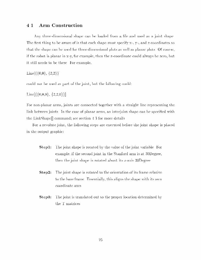
4.1 Arm Construction
Any three-dimensional shape can be loaded from a �le and used as a joint shape.
The �rst thing to be aware of is that each shape must specify x-, y-, and z-coordinates so
that the shape can be used for three-dimensional plots as well as planar plots. Of course,
if the robot is planar in x-y, for example, then the z-coordinate could always be zero, but
it still needs to be there. For example,
Line[ff0,0g, f2,2gg]
could not be used as part of the joint, but the following could:
Line[ff0,0,0g, f2,2,0gg]
For non-planar arms, joints are connected together with a straight line representing the
link between joints. In the case of planar arms, an interjoint shape can be speci�ed with
the LinkShape[] command; see section 4.3 for more details.
For a revolute joint, the following steps are executed before the joint shape is placed
in the output graphic:
Step1: The joint shape is rotated by the value of the joint variable. For
example, if the second joint in the Stanford arm is at 30Degree,
then the joint shape is rotated about its z-axis 30Degree.
Step2: The joint shape is rotated to the orientation of its frame relative
to the base frame. Essentially, this aligns the shape with its own
coordinate axes.
Step3: The joint is translated out to the proper location determined by
the T matrices.
25

Step4: If the robot is planar, then the appropriate coordinate is
dropped, and two-dimensional plots result when drawing the
robot. For example, an x-y planar robot would have its z-
coordinate dropped.
The steps for a prismatic joint are very similar:
Step1: The joint shape is rotated to the orientation of its frame relative
to the base frame. Essentially, this aligns the shape with its own
coordinate axes.
Step2: The joint is translated out to the proper location determined by
the T matrices.
Step3: If the robot is planar, then the appropriate coordinate is
dropped, and two-dimensional plots result when drawing the
robot. For example, an x-y planar robot would have its z-
coordinate dropped.
4.2 Design Guidelines for Joints
To design a joint graphic which will work with Robotica, the following points should
be observed:
1) The joint should be laid out in the coordinate system of the base frame. This is
why all of the rotations are done to align the shape with its local coordinate system.
2) A revolute joint probably should have its origin centered around (0,0,0) in the base
frame so that the rotations applied will produce the expected results.
3) Any joint shape, even if planar, should include a value for all three coordinates
(x,y,z). Thus the components of an x-y planar prismatic joint could look like
Line[f f0,1,0g, f1,1,0g, ...g]
26

and not like
Line[f f0,1g, f1,1g, ...g]
The packages Shapes.m and Polyhedra.m can provide building blocks for custom joint
shapes. These two standard Mathematica packages contain functions for generating and
manipulating many types of shapes such as cones, cylinders, and spheres. In addition,
the packages include functions that can stretch, rotate, and translate shapes, as well as
convert a solid to a wireframe. To create a custom joint with Shapes.m and Polyhedra.m,
the functions would be used to generate a series of shapes which would be assigned to
some variable in Mathematica. When the design is complete, the variable should be
written to a �le and loaded with PrisJoint[] or RevJoint[].
4.3 An Example
Creating a new joint shape is relatively easy; solids from the package Shapes.m are
the most useful is de�ning new joints. Assuming that the Shapes.m package has been
loaded, the commands given below will create a new revolute shape that looks like a
cylinder. This shape di�ers from the default revolute shape in that it is rendered as
a solid with hidden surface elimination, which makes it more realistic looking. A solid
generated with Shapes.m can be converted to wireframe with the WireFrame[] command;
see the Shapes.m �le for more information.
rev = Cylinder[];
rev = A�neShape[rev, .5, .5, .5]; (* make it half size *)
rev >> newrev (* save the shape in a �le *)
Other shapes can be incorporated into the joint design as well. For example, adding a
pyramid that points in the direction of motion for a prismatic joint is relatively straight-
forward. The following commands create a new prismatic joint with a square base and a
pyramid whose apex indicates direction of motion:
base = Cylinder[1,1,4] (* 4 sided cylinder is a cube *)
point = Cone[1,1,4] (*4 sided cone is a pyramid *)
27

base = A�neShape[base, .5, .5, .5]
point = A�neShape[point, .5, .5, .5]
point = TranslateShape[point, 0,0,1] (* put the pyramid on top of the cube *)
pris = base, point (* create a list with both shapes *)
pris >> newpris (* save the shape in a �le *)
Figure 4.4 shows the new prismatic joint shape and Figure 4.5 shows how the new
joints appear in a graphic. Of course, the commands PrisJoint[] and RevJoint[] must be
used to load the new joint shapes before rendering.
Figure 4.4: New prismatic joint.
4.4 Planar Arm Interjoint Shapes
Planar arms can be drawn with link shapes connecting the joint shapes. The function
LinkShape[] loads a shape de�nition from a �le (or if no �lename is given, uses a simple
rectangular shape). The function ClearLinkShape[] causes Robotica to clear the link
de�nition and use a line to represent links.
28

Figure 4.5: Stanford arm with new joint shapes.
Figure 4.6 shows a two-link planar arm with the standard revolute joint shape and
link shape. Figure 4.7 shows the same arm with a diamond link shape; this shape was
stored in a �le as:
Line[ff0,0,0g, f.5,.5,0g, f1,0,0g, f.5,-.5,0g, f0,0,0gg]
Much of the confusion in creating a link shape stems from the fact that the shape is
scaled by either ai in x or di in z before being placed in the graphic (where i is the joint
number). If the ai parameter is non-zero, then the link shape is scaled by ai in x. This
means that the link shape should begin at x=0 and end at x=1 so that after scaling, the
link shape starts at x=0 and ends at x=ai. This was the case for the two link planar
arm in Figure 4.6 and Figure 4.7. The situation is similar for a non-zero di except that
the arm is scaled in z. These scalings must be done in order to insure that the links and
joints appear connected on the graphic.
29

Figure 4.6: Arm with standard shapes.
Figure 4.7: Arm with new link shape.
30

4.5 Animation and other Options
To produce animations with Robotica, the package Animation.m must be loaded; this
package is provided by Wolfram Research as part of the standard Mathematica system.
Specifying the animate option to the various procedures will suppress the generation of
the composite image and use each frame to generate a frame by frame animation. Writing
all of the frames to the animation program is not a quick process; eventually, however,
the animation output will stop ashing and the frames will ow smoothly together. Each
frame of the animation must have consistent plot ranges so that the animation ows
smoothly. The x, y, and z ranges are set with the SetRanges[] command which forces
each part of the animation to include x, y, and z values as speci�ed by the ranges. In
addition, boxes can be drawn around each frame if the frame option is speci�ed. Usually,
however, adding the frame clutters the image too much to be useful.
31

CHAPTER 5
DYNAMICS
Another feature included in Robotica is the ability to compute the Euler-Lagrange
dynamics description of a robot. Robotica computes the mass matrix, Christo�el symbols,
C matrix, and the gravity vector when an input �le with dynamics data is loaded and
the appropriate commands are executed.
5.1 Loading a Robot
The �rst step in the process of generating the equations is loading the data �le
representing the robot. The Robotica command \DataFile[]" is used for this purpose; it
can be used in two ways: DataFile[\�lename"] or DataFile[].
The �rst method speci�es the �lename from which to load the data; it must be a
quoted string. For example, DataFile[\newtwo"] loads the �le \newtwo" if it exists in
the �le system. Entering DataFile[] without the �lename parameter will cause Robotica
to prompt for the �lename. Simply type the �lename without quotes in response to the
query and Robotica will load the �le.
In[2] := DataFile[\newtwo"]
or
In[2] := DataFile[]
Enter Data File Name : newtwo
If the data �le is in the correct format and DataFile[] successfully reads the parameters,
a table will be displayed showing what Robotica has stored internally from the �le. If the
�le does not exist or is incorrectly formatted, a message will be displayed to that e�ect,
and Robotica will not store anything.
32

Figure 5.1 shows what a successful read operation looks like.
0
0
0
0
0
0
0
0
I1
0
0
0
0
0
0
0
0
I2
Link
1
2
mass
m1
m2
com vector
[-a1/2, 0, 0]
[-a2/2, 0, 0]
Inertia[1]=
Inertia[2]=
In[2]:= Data�le[]
Enter data �le name: newtwo
State Reset...
Kinematics Input Data|||||Joint
1
2
Type
revolute
revolute
a
a1
a2
alpha
0
0
d
0
0
theta
q1
Dynamics Input Data||||{
q2
Gravity vector: [0,g,0]
Figure 5.1: Successful read operation.
5.2 Generating the Equations
Once the data �le has been loaded, a two-step process is required to generate Euler-
Lagrange dynamics; �rst, FKin[] must be successfully run to compute the forward kine-
matics. See Chapter 3 for complete information on this process. The second step is to
run ELDynamics[], the command which will produce the dynamics information. ELDy-
33

namics[] does not take any parameters. Figure 5.2 shows the generation of dynamics
equations with the input data from Figure 5.1.
In[5]:= ELDynamics[]
Mass Matrix MU(2 x 2) Formed. No Trigonometric Simpli�cation
Christo�el Symbols Formed
C Matrix CM(2 x 2) Formed
Gravity Vector G(2 x 1) Formed
Figure 5.2: Results of ELDynamics[].
Due to its immense complexity, the mass matrix produced (MU) will not be simpli-
�ed unless it is explicitly requested with SimplifyExpression[MU] or SDynamics[]. For
arms with even a small number of links this process could take a very long time due
to the symbolic nature of the quantities involved. If there are only a few elements of
interest in the mass matrix, they can be simpli�ed independently. For example, Simpli-
fyExpression[MU[[1,1]]], reduces only the �rst element. The Christo�el symbols and C
matrix will, in general, also need to be simpli�ed. Running SDynamics[] will simplify,
using SimplifyExpression[], all of the dynamics quantities generated and will also display
which elements are currently going through the simpli�cation process.
5.3 Printing Results
Once the dynamics equations have been generated, showing the results is accom-
plished through a set of display functions provided within Robotica. EPrint[] is one such
function; it takes up to three parameters: the matrix to be displayed (required), a text
label to print alongside the matrix (required), and a �lename in quotes in which to save
the matrix (optional). Figure 5.3 shows how EPrint[] is used to display the elements of
the simpli�ed mass matrix.
34

a1 a2 m2 Cos[q2]
2
a2 m22
4
a2 m22
4
a1 a2 m2 Cos[q2]
2
a2 m22
4
a1 m12
4
a2 m22
4
Mass matrix[2,1] = I2 +
Mass matrix[1,2] = I2 +
Mass matrix[2,1] = I2 +
Mass matrix[1,1] = I1 + I2 +
+
+
+ a1 m2 + + a1 a2 m2 Cos[q2]
In[6]:= EPrint[M, \Mass matrix"]
Figure 5.3: The elements of the mass matrix.
It is sometimes convenient to change the trigonometric notation to be somewhat
more succinct. The function SimplifyTrigNotation[] takes no parameters and modi�es
the display of Sin[] and Cos[] to an abbreviated form. Figure 5.4 shows the results of
running SimplifyTrigNotation[].
The Christo�el symbols are stored in a three-dimensional array called c. They can
be examined by entering c with a subscript or by using the CPrint[] function. Figure 5.5
shows how to examine individual elements. Other quantities of interest that can be
displayed include the Jacobians Jvc and Jwc. For example, Figure 5.6 shows the Jvc
matrices for the two-link robot. In addition, G, the gravity vector, can be displayed with
a simple call to MPrint[]. Figure 5.7 shows G for the two-link robot.
5.4 Summary
In summary, there are only three steps required to generate the Euler-Lagrange
dynamics information:
1) Run DataFile[] to load the set of Denavit-Hartenburg parameters.
2) Run FKin[] to make Robotica do the forward kinematics.
3) Run ELDynamics[] to generate the dynamics information.
35

Once these steps are performed, any of the display functions can be invoked to show
the results. SimplifyExpression[] can also be used at this point to simplify any required
information.
-(a1 a2 m2 Dq2 S2)
2
2
a1 a2 m2 Dq1 S2
2
-(a1 a2 m2 Dq1 S2) a1 a2 m2 Dq2 S2
2
In[7]:= SimplifyTrigNotation[]
C Matrix[2,2] = 0
C Matrix[1,1] =
C Matrix[2,1] =
C Matrix[1,2] =
In[8]:= EPrint[CM, \C Matrix"]
Figure 5.4: Results of running Simplify TrigNotation[].
36

In[10]:= c[[1,1,1]]
Out[10] = 0
In[11]:= c[[1,2,1]]
In[12]:= c[[1,1,2]]
Out[12]=a1 a2 m2 S2
2
Out[11] =-(a1 a2 m2 S2)
2
Figure 5.5: Examining the Christo�el symbols.
a1 C1
-(a1 S1)
2
2
a2 S12
2
2
a2 C12
-(a2 S12)
2
a2 C12
0
2
Jvc1[2,1] =
Jvc1[3,1] = 0
Jvc1[1,2] = 0
Jvc1[2,2] = 0
Jvc1[3,2] = 0
Jvc1[1,1] =
Out[16]=
Jvc2=
-(a1 S1) -
a1 C1 +
0
In[14]:= EPrint[Jvc[1], \Jvc1"]
In[16]:= MPrint[Jvc[2], \Jvc2 = "]
Figure 5.6: The Jvc matrices.
37

a1 g m1 C1
2
a2 g m2 C12
2
2
a2 C12)
Out[25] =
Gravity Vector g =
+ g m2 (a1 C1 +
In[25]:= MPrint[G, \Gravity Vector g = "]
Figure 5.7: G, the gravity vector.
38

CHAPTER 6
DYNAMICS RESPONSE COMPUTATION
Complementing the ability to compute the dynamics equations governing a robotic
arm is the ability to solve the equations numerically for the time response of the joint
variables, given an input torque. The torques are supplied to Robotica through an input
�le, which de�nes the elements of the torque vector, as well as other variables which may
be used in the de�nition of the torque vector. The time response, once computed, can
then be saved in SIMNON compatible format for later analysis with Simplot[], SimDrive[],
or SIMNON itself. See SimDrive[] in the command reference for a description of the �le
format. Before any of these calculations can proceed, however, both ELDynamics[] and
SDynamics[] must have been run.
6.1 De�ning the Torque Vector
The input torque vector represents � inM(q)�q+C(q; _q) _q+g(q) = � , where � =
266666664
�1
:
:
�n
377777775,
a vector containing a number of elements equal to the number of degrees of freedom in
the robot. GetInputTau[] is the function responsible for reading a de�nition of the input
torque; use a �lename parameter to obtain an input vector from a �le, or use no parameter
to set the input torque vector to all zeros. For example,
GetInputTau[\tau1"]
reads the torque de�nition from the �le \tau1" and
39

GetInputTau[]
sets the torque vector to all zeros.
The input �le format is rather exible, as it can contain variable name and function
de�nitions that can be used in later assignments within the �le. Mathematica interprets
all of the expressions found in the �le, and keeps track of them so that they may be
modi�ed later. Note that de�nitions loaded from a �le can interfere with user-de�ned
variables; essentially, the result of reading the input �le is the same as if each line had
been entered directly to Mathematica. Consider the input �le in Figure 6.1.
q1r = 3Sin[t]
q1dr = 3Cos[t]
q1ddr = -3Sin[t]
tau[1] = k1(q1r - q1[t]) + k2(q1dr - q1'[t]) + q1ddr
Figure 6.1: Reading the input torque vector.
The variables q1r, q1dr, and q1ddr are de�ned in the �rst three lines, then later used
in the de�nition of the �rst element of the tau vector, tau[1]. The only requirements on
the format of the input �le are that each element of the tau vector is assigned with the
following semantics: tau[n] = EXPRESSION, and that there are n entries in tau, one for
each degree of freedom. The example in Figure 5.1 de�nes the necessary element in the
tau vector for a single link arm, it applies feedback to try to force the arm to track a Sine
wave of amplitude 3. Note that the variables k1 and k2 are left unde�ned; these must
be assigned values before the response function can be called. They are left as symbols
in the input �le to allow greater exibility of parameter adjustment.
6.2 Calling Response
Assuming that the dynamics have been generated with ELDynamics[], the response
can be calculated with a call to Response[]. First, however, all symbolic entries must
be assigned numerical values; this includes setting the inertias, link masses, etc. The
following examples use the tau vector for the one degree of freedom revolute arm. There
40

are two parameters to response, each a list. The �rst list can contain two or three
numbers: the �rst is the start time of the response, the second is the end time of the
response, and the last is the maximum number of steps Response[] should take when
calculating solutions. The start and stop times are required; the number of steps should
be set to a large value if the total response time is long. The default number of steps
is 500. One way to handle choosing the number of steps to specify is to assign it some
arbitrary large value, e.g., 1000000, although the number of steps can be determined by
running Response[], then adjusting the steps to a greater value if the following message
appears:
NDSolve::mxst: Maximum number of steps reached at the point xxx.
The second list contains the initial conditions used when solving the di�erential equa-
tions. In general, there should be 2n initial conditions, where n is the number of degrees
of freedom (since the equations involve up to second derivatives for each joint parameter).
The following is a valid call to Response[]:
Response[f0,5g, fq1[0]==0, q1'[0]==0g]
This calculates the time response of the one link example over the time range 0 to 5
(using the default number of steps), with the input torque as de�ned in Figure 6.1. Notice
the format of the initial condition assignment. It is important that double equal signs be
used when setting these parameters; if a single equal sign is used, Mathematica assumes
that an assignnment is being made directly to the variables, rather than a conditional
test.
6.3 Saving Results
After Response[] has been run and solutions have been generated, they may be
saved to a �le in SIMNON compatible format for analysis. Putting the results in a �le is
accomplished with the SaveResponse[] function. Either two or three parameters are given
to SaveResponse[]; the �rst parameter is a string containing a �le name in which to save
the data; this parameter is required. The second parameter is a list containing the time
41

range from the solution to save; it is also required. The time range given must lie within
the range initially solved for with Response[], of course. The third paramter is optional,
and speci�es the size of time step to take when saving the data; it defaults to 0.1. A
value for the joint variables will be stored starting at the start time, incremented by the
step, and ending at the stop time. The following is a valid call to SaveResponse[]:
SaveResponse[\sinres", f0,5g, 0.05]
6.4 Viewing Results
Once the solutions have been saved, the functions SimDrive[] and SimPlot[] can be
used to visualize the results. Assuming that we have generated the response and saved
it to �le \sinres" as described above, SimDrive[] can be called to load the data set into
memory. SimPlot[] can then be used to display the joint trajectory. For example,
SimDrive[\sinres"]
SimPlot[t, fq1g]
results in the graph of q1 shown in Figure 6.2. All of the options available from SimDrive[]
can be speci�ed, of course. For example, SimDrive[\$", farm , animateg] would show an
animation of the arm respsonding to the input torque. Some of the more useful options
include:
trace: Show a plot of the end e�ector location.
arm: Draw the arm graphics as the arm moves in response to the
input data.
animate: Take all of the generated frames, and show them sequentially
in movie fashion. The animation can be shown again with
ShowAnim[], or saved with SaveAnim[].
42

Figure 6.2: Joint parameter q1 tracking a Sine wave.
6.5 Two-Link Example
Figure 6.3 shows the tau �le de�nition of a controller that tries to make a two-link
arm with revolute joints move in a circle centered about (2,2). The DH description is
given in Figure 3.1. The input tau �le de�nes the circle in Cartesian space in the �rst
two lines, then proceeds to de�ne quantities which are used as references in the control
equations. The parameters om, kp1, kp2, kd1, and kd2 are set at the end of the �le,
although they could be assigned values at any time prior to the running of Response[].
In addition, the values a1, and a2 were set to 3, m1 set to 10, m2 set to 5, g set to 9.8,
I1 set to 0.833, and I2 set to 0.417.
Note that the de�nitions of tau[1] and tau[2] include quantities that are generated by
the dynamics commands, namely, elements of the simpli�ed mass matrix (M), elements
of the simpli�ed C matrix (CM), and elements of the gravity vector (G).
The commands given to calculate the response over the time period 0,10 and save the
response in a �le called \circ1" are shown below.
In[25]:= Response[f0,10,100000g, fq1[0]==0, q2[0]==0, q1'[0]==0, q2'[0]==0g]
43

Solving equations...
Out[25]=
ffq1 -> InterpolatingFunction[f0,10g, <>], q2 -> InterpolatingFunction[f0,10g, <>]gg
In[26]:= SaveResponse[\circ1", f0,10g]
Next, SimDrive[] was used to load the data; the following command was used:
In[30]:= SimDrive[\circ1"]
With the data in memory, the following plots were created: the values of the joint
variables, the location of the arm, and the trace of the end e�ector location. The com-
mands used were:
SimPlot[t, fq1,q2g] to generate Figure 6.4,
SimDrive[\$", farmg], to generate Figure 6.5, and
SimDrive[\$", ftraceg] to generate Figure 6.6.
44

j11 = -a1*Sin[q1d] + a2*Cos[q1d+q2d]
j12 = -a2*Sin[q1d+q2d]
j21 = a1*Cos[q1d] + a2*Cos[q1d+q2d]
j22 = a2*Cos[q1d+q2d]
detj = a1*a2*Sin[q2d]
v1d = (1/detj) * (j22*vx - j12*vy)
v2d = (1/detj) * (-j21*vx + j11*vy)
jd11 = -a1*Cos[q1d] * v1d - a2*Cos[q1d+q2d] * (v1d+v2d)
jd12 = -a2*Cos[q1d+q2d] * (v1d+v2d)
jd21 = -a1*Sin[q1d] * v1d - a2*Sin[q1d+q2d] * (v1d+v2d)
jd22 = -a2*Sin[q1d+q2d] * (v1d+v2d)
bbx = ax-jd11*v1d - jd12*v2d
bby = ay-jd21*v1d - jd22*v2d
aq2 = a2d + kp2 * (q2d - q2[t]) +kd2*(v2d - q2’[t])
tau[2] = M[[2,1]]*aq1 + M[[2,2]]*aq2 + CM[[2,1]]*q1’[t] + G[[2]]
a1d = (1/detj) * (j22*bbx - j12*bby)
a2d = (1/detj) * (-j21*bbx + j11*bby)
aq1 = a1d + kp1 * (q1d -q1[t]) +kd1*(v1d - q1’[t])
om=1
kp1=400
kp2=400
kd1=40
kd2=40
x = 2+Cos[om*t]
y = 2+Sin[om*t]
vx=-om*Sin[om*t]
vy= om*Cos[om*t]
ax = -om * om * Cos[om*t]
ay = -om * om * Sin[om*t]
DD = (x*x + y*y -a1*a1 -a2*a2) / (2*a1*a2)
q1d = ArcTan[x,y] - ArcTan[a1+a2*Cos[q2d], a2*Sin[q2d]]
q2d = ArcCos[DD]
tau[1] = M[[1,1]]*aq1 + M[[1,2]]*aq2 + CM[[1,1]]*q1’[t] + CM[[1,2]] * q2’[t]+ G[[1]]
Figure 6.3: Circular motion control de�nitions.
45

Figure 6.4: Joint variables as a function of time.
Figure 6.5: Arm location from circular controller.
46

Figure 6.6: End e�ector location from circular controller.
47

CHAPTER 7
MANIPULABILITY
Another unique feature of Robotica is its ability to compute and display the ma-
nipulability ellipsoids for a robot described by Denavit-Hartenburg input parameters.
Complete information on manipulability can be found in [4]. The manipulability ellip-
soids are related to how quickly the end e�ector can move in a given direction. For a
planar arm, the ellipsoids are ellipses in a plane, and the distance from the center of the
ellipse to the ellipse is one of the factors that determines how quickly the arm can move in
that direction. The case is similar in three-dimensional space, except that the ellipse is an
actual three-dimensional ellipsoid. Of course, the manipulability also depends on other
factors such as the strength of the joint motors, etc. The manipulability measures that
can be computed are valuable pieces of information to have when planning the workspace
in which the robot will operate.
7.1 Generating the Ellipsoids
RElp[] is the function responsible for the calculation and display of the ellipsoids.
The format of the RElp[] command is:
In[5] := RElp[vars, options]
This function calculates and displays manipulability ellipsoids for a robot when a range
of input parameters is speci�ed. First, of course, a robot must have been loaded with
DataFile[]; in addition, FKin[] must have been run. (RElp[] makes heavy use of the
Jacobian and T matrices calculated with FKin[]).
The �rst argument, called vars above, is a list containing a series of sublists. The
sublists are of the following form: fvariable, start, endg, and vars is a sequence of these:
48

ffvariable1,start,endg, fvariable2,start,endg,. . .g. The sublists specify three things:
�rst, a Denavit-Hartenberg parameter for the variable such as d1, q2, and a1 (these
are the variable entries in the input parameter �le); second, the starting value for that
variable; and �nally, the ending value for that variable. For example, fd1, 3, 8g causes
the Denavit-Hartenberg parameter d1 to run from 3 to 8. The range from start to end
is, by default, divided into �ve pieces, although this can be modi�ed by appending the
number of divisions to the end of the variable list. For example, to use eight steps, the
variable list would look like this: f fq1, 3, 4g, . . . , fdn, 0,3g, 8g. It should be noted that
angular parameters are speci�ed in radians; however, using the built-in degrees to radians
converter, Degree, a value can be given in degrees, e.g., fq2, 30 Degree, 180 Degreeg.
The converter can be placed anywhere after the value, and must be spelled with a capital
\D."
Not all of the input parameters that were speci�ed in the input �le have to be assigned
a range; however, each must have some de�nite numerical value. If there is a Denavit-
Hartenberg parameter that will have a constant value, it can be assigned with a normal
Mathematica command, for example,
In[6] := d3 = 5
This de�nition can be cleared later with Clear[d3], at which time the variable will be
purely symbolic again. Variables should be cleared before loading a new robot as well.
The variable list and constant parameter assignments should leave no variables in the
Jacobian or T matrices with purely symbolic values.
7.2 Options
The options are also given in the form of a list. The available options are:
single: RElp[] plots only the ellipsoid at the start values of the parameters in
the sublists.
frame: Put a frame around graphics.
49

animate: Take all of the generated frames and show them sequentially
in movie fashion. The animation can be shown again with
ShowAnim[] or saved with SaveAnim[].
measures: Print a set of manipulability measures for each ellipsoid (i.e., at each
step of parameter values). The measures include the actual axes cal-
culated, volume of the ellipsoid, eccentricity (closer to one means more
spherical), minimum radius, and the geometric mean of the radii (a
sphere with this radius has the same volume as the ellipsoid; see Chap-
ter 4 of [4]).
monly: Causes RElp[] to print only manipulability measures; no graphics are
generated.
\�le": Save the ellipsoid measures in a �le called \�le" if either measures or
monly is speci�ed in the option list. The �lename must be a string (e.g.,
\measures") which represents a valid �lename on the system being used.
If the �le already exists, the ellipsoid measure information is appended
to the end of the �le; otherwise, a new �le is created. Also, once a
�le has been speci�ed, it becomes the default output �le. To specify
that output should go to the default �le, use \$" as the �lename. If no
�lename is given, the ellipsoid measure information is displayed on the
screen only.
scale: Specify this option to scale the ellipsoids such that the largest axis is
always two units long. This helps to keep the plot from becoming too
cluttered with overlapping ellipses.
print: If Mathematica has a LaserPrint function de�ned, it will be used to
print the graph.
50

xprint: Using this option assumes that Mathematica is running under X-
windows; including xprint in the options list will attempt to utilize
the X-windows utilities xpr and xwd to allow the user to pick a graph-
ics output window to save as a postscript compatible �le. The output
�le will be called \xrelp.out."
mprint: This uses the internal Mathematica command Display[] to convert the
output graphic to a raw postscript �le. Some extra processing may
have to be done before the �le is sent to a postscript output device.
See [2] for details. The output �le will be called \mrelp.out."
Options must be in a list and can be given in any order. For example, RElp[an, fscale,
singleg] causes RElp[] to draw a single, scaled ellipsoid at the start values of the param-
eters in the list an.
If no arm graphics have been loaded, simple lines will be used to show the arm. See
Chapter 4 for information on the use of more complicated arm graphic representations.
Also, a variable called manplot is created to hold the current manipulability plot. It
can be viewed at any time after a plot has been generated with Show[manplot]. Any
of the various display options available from the Mathematica function Show[], (e.g.,
ViewPoint) can be used when viewing the plot.
7.3 Examples
Figure 7.1 shows a sample of the output produced by RElp[] for a simple two-
link revolute joint, prismatic joint arm. First, of course, the data �le was loaded with
DataFile[]. Next, a prismatic joint shape was loaded with PrisJoint[] and a revolute joint
shape with RevJoint[]. The parameter a1 was set to 5, and the command RElp[f fq1, 0,
90Degreeg, fd2, 3, 8g g, fsingleg] was used to generate the graph.
51

Figure 7.1: Planar manipulability example.
When many ellipsoids are drawn, they tend to obscure one another on the graph.
Specifying the option scale normalizes the size of each ellipsoid such that the largest axis
is 2 units long; this is useful for judging the relative amount of manipulability in each
con�guration. RElp[f fq1, 0, 90Degreeg, fd2, 3, 8g g, fscaleg] generated the results
shown in Figure 7.2.
52

Figure 7.2: Scaling the ellipsoids.
The input data �le for a more complicated robot is shown in Figure 7.3. The manip-
ulability for the arm was calculated with RElp[ffq1, 0, 180Degreeg, fd3, 2, 8g, 3g]. The
variable q2 was �xed at 50�. Figure 7.4 shows the results.
53

DOF
joint1
a1
alpha1
d1
theta1
joint2
a2
alpha2
d2
theta2
joint3
a3
alpha3
d3
theta3
=
=
=
=
=
=
=
=
=
=
=
=
=
=
=
=
3
revolute
0
-Pi/2
5
q1
revolute
0
10
q2
prismatic
0
0
d3
-Pi/2
Pi/2
Figure 7.3: Three-link example.
Figure 7.4: Three-link nonplanar example.
54

With three-dimensional pictures, it can be di�cult to see just what is happening
as the robot moves. With the ViewPoint option, it is possible to view the plot from
any point, allowing a more reasonable perspective to be presented. Figure 7.5 shows
the results of moving the viewpoint with Show[manplot, ViewPoint->f-1,-0.5,0g]. Even
with the ability to adjust the viewpoint, it is usually more informative to generate the
numerical measures of manipulability rather than extracting this information from the
graphic. See Chapter 4 of [4] for more information on manipulability.
Figure 7.5: A change of ViewPoint.
55

CHAPTER 8
EXTERNAL SIMULATION COMPATIBILITY
Robotica has the ability to read data from external simulations such as SIMNON [1]
and generate graphical output showing the result of applying the joint motion data in
the �le to the current robot. In addition, the data in the simulation �le can be displayed,
plotted, and printed in numerous ways.
There are two functions provided to handle simulation compatibility. The �rst, Sim-
Drive[], begins by reading a simulation input �le. It then graphically shows the results of
applying the joint parameter values speci�ed by the simulation �le to the current robot.
The second command, SimPlot[], is used to plot the simulation input data in familiar
x-y format by specifying the various quantities to be graphed.
8.1 Loading Simulation Data
The Robotica function SimDrive[] is used to read the simulation output �le { it
must adhere to the format shown in Section 8.2. If necessary, a text editor can be used
to modify the �le so that it matches the required format. SimDrive[] requires that an
input �le of Denavit-Hartenberg parameters has been created for the robot that the
simulation output will drive. This input �le should be loaded with DataFile[] and the
forward kinematics should then be generated with FKin[]. The format for the SimDrive[]
command is:
SimDrive[�lename, options]
The �lename must be in quotes and designates the �le to acquire input from. Once the
data are read in, the data in each set are used to update robot arm parameters, and
56

the graphics are generated and output. The data and variable list is stored for further
analysis. To indicate another plot with the same data, use \$" as the �lename.
The options for SimDrive[] are held in a list which may contain any of the following:
trace: Show a plot of the �nal coordinate frame location.
arm: Draw the arm graphics as the arm moves in response to the input data.
frame: Put a frame around graphics.
animate: Take all of the generated frames, and show them sequentially
in movie fashion. The animation can be shown again with
ShowAnim[], or saved with SaveAnim[].
print: If Mathematica has a LaserPrint function de�ned, it will be used to
print the graph.
xprint: Using this option assumes that Mathematica is running under X-
windows; including xprint in the options list will attempt to utilize
the X-windows utilities xpr and xwd to allow the user to pick a graph-
ics output window to save as a postscript compatible �le. The output
�le will be called \xsim.out."
mprint: This uses the internal Mathematica command Display[] to convert the
output graphic to a raw postscript �le. Some extra processing may
need to be done before the �le is sent to a postscript output device.
See the Mathematica users' manual for details. The output �le will be
called \msim.out."
A new image of the robot is drawn whenever a speci�ed sample time has elapsed (see
Section 8.2, the default being .2 units. A di�erent time can be speci�ed by appending a
number to the options list. For example, SimDrive[\simnon", ftrace, .1g] would update
the plot whenever more than .1 time units elapsed.
57

If neither arm nor trace is a member of the options list, or an option list is not given
at all, SimDrive[] will merely read the input data set and not produce any graphics; of
course, the data set is now available to SimPlot[] for analysis.
8.2 Simulation Input File Format
The input �le should be in the following format (the line numbers are for reference
only, they should not actually exist in the input �le).
[1] 00 t d1 q1
[2] 00
[3] 0 1 0.02
[4] 1 1 0.04 ...
SIMNON directly supports this output format. Line [1] is a comment line containing the
names of the variables for which data is listed in this �le. In the above example, data
will be speci�ed for t, d1, and q1. It is always assumed that t will be the �rst of the
input parameters; it is used in the determination of elapsed time mentioned above. The
third line is just a comment line and is ignored; there can be any number of comment
lines following the variable list.
The data are listed after the last comment line, with each line containing one set of
input values. Thus, if there are three input variables, each line will contain three values.
For example, Line [3] would assign 0 to t, 1 to d1 and 0.02 to q1. The time parameter t
is always assumed to be the �rst variable in the list.
8.3 Plotting Simulation Data
The other Robotica function dealing with external simulation data is called SimPlot[].
Its format is shown below:
SimPlot[indep, deplist, options]
SimPlot[] plots data loaded through the function SimDrive[]. The �rst parameter is
the independent variable, i.e., the x-axis. The second parameter is a list of dependent
58

variables to be plotted against the independent variable. For example, SimPlot[t, fq1g]
plots t vs. q1, and SimPlot[t, fq1,q2g] plots t vs. q1 and q2.
The parameters indep and deplist are required, and options is optional. The options
must be in a list, and can include print, xprint, and mprint. These functions as described
in Section 7.1; the �les produced, however, are called \xsimplot.out" for xprint, and
\msimplot.out" for mprint.
8.4 Examples
Assume SIMNON has been used to simulate the e�ect of a controller attempting to
move a two degree of freedom planar arm in a circle. The joint variable data have been
stored in the �le \simnon." Figure 8.1 shows how the �le would be loaded.
Got header...
Attempting to read values for these parameters:
t
q1
q2
q1d
q2d
Working...
Data �le loaded...
In[4]:= SimDrive[\Simnon"]
Figure 8.1: Loading a SIMNON �le.
Now, assuming that a two degree of freedom planar robot has been loaded, with joint
variables matching those speci�ed in the SIMNON data (q1 and q2 here), we can see
the e�ects of the controller as speci�ed by the data set. For this simulation, a1 and a2
were set at 5. For example, entering SimDrive[\$", farmg] results in the output shown
in Figure 8.2.
59

Figure 8.2: Two link planar arm driven with dataset.
Note the use of \$" to tell SimDrive[] to utilize the data currently loaded and the
drawing of a revolute arm shape loaded with RevLink[]. Figure 8.3 shows a plot of the
origin of the last coordinate frame, which makes the circular motion much easier to see.
This plot was generated with SimDrive[\$", ftraceg].
Now that the data are loaded, we can plot the information using SimPlot[]. Figure 8.4
shows an example of plotting time, t, against q1 and q2. The command used to generate
this graph was SimPlot[t, fq1, q2g].
Finally, Figure 8.5 shows a plot of q1 against q2, produced by SimPlot[q1, fq2g].
60

Figure 8.3: Plot of the end e�ector location.
61

Figure 8.4: Time, t, versus q1 and q2.
62

Figure 8.5: Joint parameter q1 versus q2.
63

CHAPTER 9
ROBOTICA FRONT END
The Robotica front end (RFE) is a graphical user interface for Robotica that allows
the user to access the capabilities of the package without having to deal directly with
Mathematica. The front end insulates the user from the inconvenience and idiosyncrasies
associated with typing commands directly and provides an environment far easier to use
than the standard Mathematica textual interface. The interface was written in C using
the Open Look widgets [5], [6].
9.1 The Structure of RFE
The front end (Figure 9.1) consists of four major elements: a menu bar, located across
the top of the window (it contains the �le, fonts, and packages menus); a Mathematica
output window, located in the left half of the window; a function selection window,
located in the right half of the window; and a command entry �eld, located below the
Mathematica output window.
9.2 Menu Bar
The menu bar contains pulldown menus called �le, fonts, and packages. The menus
o�er convenient access to features which are frequently needed.
9.2.1 File
Activating the �le menu displays the following choices: Clear Text, Abort, and Quit.
Selecting Clear Text erases everything in the Mathematica output window and sets the
64

Figure 9.1: Robotica Front End.
scrollbar slider back to the top, ready for new input. Interrupting an operation can be
done with the Abort selection. The currently executing Mathematica operation will be
stopped, and Mathematica will be ready for new input after the abort sequence. The
last operation available under File is Quit. Not surprisingly, this ends the session with
RFE and returns the user to the environment that existed before RFE was run.
9.2.2 Packages
This menu contains a short list of Mathematica standard packages that contain func-
tions which add exibility to Robotica. The package Animation.m, when loaded, allows
the use of the movie-like animation sequences that RElp[], ShowRobot[], etc. can gen-
erate. The other two packages, Shapes.m and Polyhedra.m, are primarily useful for
designing new joint shapes. See Chapter 4 for further information on designing joints.
65

9.3 Mathematica Output Window
When Mathematica has an output ready for display, it sends the result to RFE, and
RFE posts the output in the Mathematica output window. The window extends beyond
the limits of the screen area allocated for it, and therefore scrollbars are provided to allow
access to nondisplayed portions of the window. Figure 9.2 shows the output window
after the DataFile[] and FKin[] commands have been executed. When the display �lls,
the vertical scrollbar is automatically moved down to keep the most recent information
visible. Of course, the scrollbars can be moved to another position to display previous
output. This window consists of read-only text; to send a command to Mathematica, use
the command input line.
Figure 9.2: Output in the Mathematica output window.
66

9.4 Command Input Line
While the function selection menu provides access to all of the Robotica routines, any
function or Mathematica command can be entered on the command input line at the
bottom of the screen. When a text string is entered on the line and the <return> key
pressed, the command is sent to Mathematica, and the output is posted in the output
window. The command input line allows the processing of any Mathematica command.
For example, entering Plot[Sin[x], fx, 0, Pig] will produce a plot of Sin[x] from 0 to Pi.
In general, any Mathematica command can be executed in this way.
9.5 Robotica Function Selection Menu
The right side of RFE consists of the Robotica Function Selection Menu. In the
menu are buttons corresponding to all of the available Robotica functions. To execute
a Robotica procedure, simply click on the button that contains the function name. For
every function, a screen will pop up showing the available options as well as a \Send"
button and a \Cancel" button. If the function takes no options (such as FKin[]), the
pop-up screen contains only the \Send" and \Receive" buttons.
Figure 9.3 shows an example of the option screen for the DataFile[] function. Here,
the only parameter is a �lename; pressing \Send" transmits the function to Robotica,
while pressing \Cancel" prevents the function from being executed. Each pop-up screen
remembers what was entered the last time the function was executed, and sets the options
to those values.
67

Figure 9.3: DataFile option screen.
Figure 9.4 shows the option screen for the SimDrive[] command. The data source �eld
is for the �le name from which data are loaded, and below that are listed the various
options that can be used with SimDrive[]. Each option has a check box to its right to
indicate whether or not that option is turned on. A check mark in the box indicates
that the option will be turned on when the function is sent, while an empty box means
the option is turned o�. In Figure 9.4, the options trace, arm, and animate have been
turned on. The Value �eld is a text entry �eld used to give a value for the step parameter
described in the SimDrive[] section of Appendix A.
Figure 9.4: SimDrive option screen.
68

When entering parameters into the option screens, the delimiters that usually sur-
round items are automatically added by RFE. For example, no quotation marks are
needed around the �lename parameter in the DataFile[] option screen. As another ex-
ample, when specifying lists of parameters to RElp[] or ShowRobot[], only the individ-
ual elements inside the variable list have to have braces around them. The delimiters
around the entire list are added automatically. In other words, entering fq1,0,90Degreeg,
fd3,2,4g on the variables line will be sent to Robotica as f fq1,0,90Degreeg, fd3,2,4g g,
which has had the brace delimiters added.
The function selection menu also contains a vertical scrollbar. At this point in time,
however, all of the available functions �t on one screen, therefore this scrollbar always
stays at the top. When additional functions are added, the scrollbar would be used to
move up and down the list of functions, which would be larger than the screen display.
69

CHAPTER 10
COMMAND REFERENCE
APrint[�le]
This function prints all the A matrices for the most recent run of FKin[]. The �le
argument is optional and speci�es a �lename in which to store the matrices. The �lename
must be a string (e.g., \matrices") which represents a valid �lename on the system being
used. If the �le already exists, the A matrix information is appended to the end of the
�le; otherwise, a new �le is created. Also, once a �le has been speci�ed, it becomes the
default �le for all of the printing functions. To specify that the output should go to the
default �le, use \$" as the �lename. If no �lename is given, the A matrices are displayed
on the screen only.
Example: APrint[\amatrix"]
ClearLinkShape[]
ClearLinkShape[] clears any de�nition for an interjoint shape. The result is that the
package will use a simple line to show links until a new interlink shape is de�ned with
LinkShape[]. ClearLinkShape[] takes no arguments.
Example: ClearLinkShape[]
70

ClearPrisJoint[]
ClearPrisJoint clears any de�nition for a prismatic joint shape. The result is that the
package will use a simple line to show prismatic joint connections until a new prismatic
link shape is de�ned with PrisJoint[]. ClearPrisJoint[] takes no arguments.
Example: ClearPrisJoint[]
ClearRevJoint[]
ClearRevJoint[] is similar to ClearPris except that it works on the revolute joint
shape de�nition. The revolute joint shape is cleared, and the system will use a line to
show revolute joint connections. A new revolute shape can be de�ned with RevJoint[].
ClearRevJoint[] function takes no arguments.
Example: ClearRev[]
CPrint[label, �lename]
CPrint[] prints, one per line, all of the elements of the C matrix (called CM in Robot-
ica). The label parameter is required and is speci�ed as a text string that will be printed
in front of the individual elements. The �lename is optional and speci�es a �lename
in which to store the elements. The �lename must be a string (e.g., \elements") which
represents a valid �lename on the system used. If the �le already exists, the matrix in-
formation is appended to the end of the �le; otherwise, a new �le is created. In addition,
once a �le has been speci�ed, it becomes the default �le for all of the printing functions.
To specify that the output should go to the default �le, use \$" as the �lename. If no
�lename is given, the elements of the matrix are displayed on the screen only.
Example: CPrint[\C symbols"]
71

DataFile[�lename]
DataFile[] loads the DH parameters from a �le. The �lename argument is optional,
but, if included, must be a string containing the name of the source �le. If the �lename
is not speci�ed, the routine will query for the name which should be typed in without
quotes.
Example: DataFile[\twodof"]
ELDynamics[]
ELDynamics[] computes the dynamics information for the current robot data set.
First, however, a data set must have been loaded with DataFile[], and the forward kine-
matics must have been computed with FKin[]. See Table 2.1 for a complete listing of the
quantities generated by Robotica.
Example: ELDynamics[]
EPrint[matrix, label, �lename]
This function prints, one per line, all elements of the matrix or vector speci�ed as
the �rst parameter, which is required. The label argument, also required (although one
could make it \" for no label), is a string that will be printed in front of individual
matrix elements. The �le argument is optional and speci�es a �lename in which to store
the matrices. The �lename must be a string (e.g., \elements") which represents a valid
�lename on the system used. If the �le already exists, the matrix information is appended
to the end of the �le; otherwise, a new �le is created. Also, once a �le has been speci�ed,
it becomes the default �le for all of the printing functions. To specify that the output
should go to the default �le, use \$" as the �lename. If no �lename is given, the elements
of the matrix are displayed on the screen only.
Example: EPrint[T[0,2], \T02=", \t�le"]
72

FKin[]
FKin computes the forward kinematics for the current robot data set. It generates
all of the A and T matrices as well as the Jacobian. See Table 2.1 for a complete listing
of quantities generated by Robotica.
Example: FKin[]
GetInputTau[�lename]
GetInputTau[] loads an input vector for the Response[] function. The �lename pa-
rameter is optional. If speci�ed, a vector de�nition is loaded from that �le, otherwise the
torque vector is set to all zeros.
Example: GetInputTau[\tau1"]
LoadAnim[�lename]
LoadAnim[] will load an animation previously saved with SaveAnim[]. Loading a
large animation may take several minutes due to the amount of rendering information
stored.
Example: LoadAnim[\anim1"]
LinkShape[�lename]
This function loads an interjoint shape from a �le to be used in planar arms. The
argument to LinkShape[] is a string containing a �lename from which to load the shape.
If no �lename is given, a standard rectangular column shape is loaded as the default link.
Currently, shapes must be three dimensional, and can include sets of Line, Polygon, and
73

Point primitives (the shapes de�ned in the package shapes.m satisfy this requirement).
See Chapter 4 for complete information about how arm graphics are handled.
Example: LinkShape["link2"]
MPrint[matrix, label, �lename]
This function prints, in matrix form, the matrix or vector speci�ed as the �rst param-
eter, which is required. The label argument, also required (although one could make it
\" for no label), is a string that will be printed in front of the matrix. The �le argument
is optional and speci�es a �lename in which to store the matrices. The �lename must
be a string (e.g., \matrix") which represents a valid �lename on the system used. If the
�le already exists, the matrix information is appended to the end of the �le; otherwise,
a new �le is created. Also, once a �le has been speci�ed, it becomes the default �le for
all the printing functions. To specify that the output should go to the default �le, use
\$" as the �lename. If no �lename is given, the matrix is displayed on the screen only.
Example: MPrint[A[2], \A2 = "]
Planar[]
Planar uses the Jacobian constructed with FKin[] and returns an integer which de-
scribes the space in which the robot moves. The return codes are:
0: The robot can not move in x, y, or z.
1: The robot moves only in x.
2: The robot moves only in y.
3: The robot moves in x and y, i.e., an x-y planar robot arm.
4: The robot moves only in z.
5: The robot moves in x and z, i.e., an x-z planar robot arm.
6: The robot moves in y and z, i.e., a y-z planar robot arm.
74

7: The robot moves in x, y, and z, i.e., a general motion in 3-space.
Example: Planar[]
PrintInputData[]
This function prints the input data set to the screen. It does not take any parameters.
Example: PrintInputData[]
PrisJoint[�lename]
This function loads a prismatic joint shape from a �le. The argument to PrisJoint[]
is a string containing a �lename from which to load the shape. If no �lename is given,
a standard rectangular column shape is loaded as the default prismatic joint. Currently,
shapes must be three dimensional, and can include sets of Line, Polygon, and Point
primitives (the shapes de�ned in the package shapes.m satisfy this requirement). See
Chapter 4 for complete information about how arm graphics are handled.
Example: PrisJoint[]
RElp[vars, options]
This function calculates and displays manipulability ellipsoids for a given robot over a
range of input parameters. First, though, a robot must have been loaded with DataFile[],
and FKin[] must have been run. The �rst argument is a list containing a series of sublists.
The sublists are of the following form: fvar, start, endg, and vars is a sequence of these:
f fvar1,start,endg, fvar2,start,endg, . . . g. The sublists specify a DH parameter such as
d1, q2, or a1 for the variable, and the starting value and ending value for that variable.
For example, fd1, 3, 8g causes the DH parameter d1 to vary from 3 to 8. The range
75

from start to end is, by default, divided into �ve pieces, although this can be changed by
appending the number of divisions to the variable list. To use eight steps, the variable
list would look like this: ffq1, 3, 4g, . . . , fdn, 0,3g, 8g. It should be noted that angular
parameters are speci�ed in radians.
Not all parameters need to be speci�ed as a range. If there is a DH parameter that
will have a constant value, it can be assigned with a normal Mathematica command (e.g.,
d3=5). The variable list and constant variables should leave no unde�ned variables in
the Jacobian or T matrices.
The options are given in the form of a list as well. The available options are:
single: Plot only one ellipsoid at the start values of the parameters.
measure: Print a list of manipulability measures for each ellipsoid. The
measures include volume, eccentricity, minimum radius, and ge-
ometric mean.
76

monly: Do not generate any graphics, only print manipulability infor-
mation (or save it to a �le).
frame: Put a frame around graphics.
animate: Take all of the generated frames and show them sequentially
in movie fashion. The animation can be shown again with
ShowAnim[], or saved with SaveAnim[].
scale: Specify this option to scale the ellipsoids such that the largest
axis is always two units long. This helps to keep the plot from
becoming too cluttered.
print: If Mathematica has a LaserPrint function de�ned, it will be used
to print the graph.
xprint: Using this option assumes that Mathematica is running under
X-windows; including xprint in the options list will attempt to
utilize the X- windows utilities xpr and xwd to allow the user to
pick a graphics output window to save as a postscript compatible
�le. The �le will be called \xrelp.out."
mprint: This uses the internal Mathematica command Display[] to con-
vert the output graphic to a raw postscript �le. Some extra pro-
cessing may need to be done before the �le is sent to a postscript
output device. See the Mathematica users' manual for details.
The �le will be called \mrelp.out."
77

\�le": Save the ellipsoid measures in a �le called \�le" if either mea-
sures or monly is speci�ed in the option list. If the �le already
exists, the information is appended to the end of the �le; other-
wise, a new �le is created. Use \$" as the �lename to indicate
that the output should go to the current default �le.
Options must be in a list, and can be given in any order. For example, RElp[an, fscale,
singleg] causes RElp[] to draw a single, scaled ellipsoid at the start values of the parame-
ters in the list an. If no arm graphics have been loaded, simple lines will be used to show
the arm. The functions RevJoint[] and PrisJoint[] can be used to load the standard joint
shapes to provide more detail.
Example: RElp[f fq1, 20Degree, 90Degreeg , 8g, fmonly, \measures"g]
Response[time, init]
Response[] calculates the time response from the dynamics equations, given an input
torque vector (loaded with GetInputTau[]). Of course, ELDynamics[] must have been
run, and all of the symbols in the equations must have been assigned numerical values.
The �rst parameter to Response[] is a list containing a start and end time over which to
solve. Additionally, a third number may be added to the end of the list; this number sets
the maximum number of steps that the algorithms can take to solve the equations. The
second parameter is a list containing a set of initial conditions that determines a unique
solution to the equations. When successful, the output can be saved with SaveResponse[].
See Chapter 6 for complete details.
Example: Response[f0,5g, fq1[0]==0, q1'[0]==0g]
RevJoint[�lename]
This function loads a revolute joint shape from a �le. The argument to RevJoint[] is
a string containing a �lename from which to load the shape. If no �lename is given, a
78

standard circular column shape is loaded as the default revolute joint. Currently, shapes
must be three-dimensional, and can include sets of Line, Polygon, and Point primitives
(the shapes de�ned in shapes.m satisfy this requirement). See Chapter 4 for complete
information on how link graphics are handled.
Example: RevJoint[\revolute"]
SDynamics[]
Since dynamics quantities are not simpli�ed when generated, this function is provided
to instruct Robotica to attempt to reduce the entire set of dynamics information. De-
pending on the number of links in the robot, this process could take a large amount of
time. Speci�c pieces of information can be simpli�ed with SimplifyExpression[] instead.
Example: SDynamics[]
SaveAnim[�lename]
SaveAnim[] will save an animation generated with RElp[], SeqShowRobot[], etc. in
the �le speci�ed. Files are usually quite large due to the amount of rendering information
stored.
Example: SaveAnim[\anim1"]
SaveResponse[�le, time, inc]
After a successful run of Response[], SaveResponse[] will store numerical values for
the solution to the dynamics equations in the �le speci�ed as the �rst parameter. The
second parameter is a list containing a start time and a stop time over which to save
the solutions. The range speci�ed must, of course, be included in the range solved for
with Response[]. The third parameter gives the time increment to be used when saving
the data; it defaults to 0.1. The �rst and second parameters are required, and the third
79

is optional. The output �le is stored in a SIMNON compatible format; as a result,
SimDrive[] and SimPlot[] can be used to plot and analyze the data.
Example: SaveResponse[\sinres", f0,5g, 0.01]
SeqShowRobot[vars, options]
This function displays the robot over a range of joint parameters; it di�ers from
ShowRobot[] in that each joint speci�cation in vars is executed sequentially rather than
simultaneously (i.e., one joint at a time moves). First, though, a robot must have been
loaded with DataFile[], and FKin[] must have been run. The �rst argument is a list
containing a series of sublists. The sublists are of the following form: fvar, start, endg,
and vars is a sequence of these: f fvar1, start, endg, fvar2, start, endg, . . .g. The sublists
specify a DH parameter such as d1, q2, or a1 for the variable, and the starting value and
ending value for that variable. For example, fd1, 3, 8g causes the DH parameter d1 to
vary from 3 to 8. The range from start to end is, by default, divided into �ve pieces,
although this can be changed by appending the number of divisions to the variable list.
To use eight steps, the variable list would look like this: f fq1, 3, 4g, . . . , fdn, 0,3g, 8g.
It should be noted that angular parameters are speci�ed in radians.
Joint parameters that have a constant value should be assigned with a Mathematica
command (e.g. d3=5) entered at the command line. The options are given in the form
of a list as well. The available options are:
80

single: Plot only one arm at the start values of the parameters.
frame: Put a frame around each graphics frame.
animate: Take all of the generated frames, and show them sequentially
in movie fashion. The animation can be shown again with
ShowAnim[] or saved with SaveAnim[].
print: If Mathematica has a LaserPrint function de�ned, it will be used
to print the graph.
xprint: Using this option assumes that Mathematica is running under
X- windows; including xprint in the options list will attempt to
utilize the X-windows utilities xpr and xwd to allow the user to
pick a graphics output window to save as a postscript compatible
�le. The output �le will be called \xrobotplot.out."
mprint: This uses the internal Mathematica command Display[] to con-
vert the output graphic to a raw postscript �le. Some extra pro-
cessing may have to be done before the �le is sent to a postscript
output device. See the Mathematica users' manual for details.
The output �le will be called \mrobotplot.out."
In addition, a variable called robotplot is created to hold the contents of the cur-
rent output of SeqShowRobot. It can displayed at any time once generated with
Show[robotplot]. Any of the various display options available from Show[] (e.g., View-
Point) can be used to view the plot.
Example: SeqShowRobot[f fq1, 20Degree, 90Degreeg, fd2, 3, 6g, fd2, 6, 3g, fq1,
90Degree, 20Degreeg , 8g]
81

SetRanges[xrange, yrange, zrange]
This function is used to set the range of display for the animation frames. To ensure
that each frame's view is consistent with every other frame, the view limits are set to
xrange, yrange, zrange. Each of the ranges should be a list containing a min, max pair.
For example, SetRanges[f-5,5g, f0,10g, f-10,0g] sets the animation views to include x
values from -5 to 5, y values from 0 to 10, and z values from -10 to 0.
Example: SetRanges[f-5,5g, f2,4g, f0,9g]
ShowAnim[]
ShowAnim shows an animation sequence that was generated with RElp[], SimDrive[],
etc. or loaded with LoadAnim[]. The package Animation.m is required for this to function
to execute.
Example: ShowAnim[]
ShowRobot[vars, options]
This function displays a robot over a range of joint parameters. First, though, a
robot must have been loaded with DataFile[], and FKin[] must have been run. The �rst
argument is a list containing a series of sublists. The sublists are of the following form:
fvar, start, endg, and vars is a sequence of these: f fvar1, start, endg, fvar2, start, endg,
. . . g. The sublists specify a DH parameter such as d1, q2, or a1 for the variable, and the
starting value and ending value for that variable. For example, fd1, 3, 8g causes the DH
parameter d1 to vary from 3 to 8. The range from start to end is, by default, divided
into �ve pieces, although this can be changed by appending the number of divisions to
the variable list. To use eight steps, the variable list would look like this: f fq1, 3, 4g,
. . . , fdn, 0,3g, 8g. It should be noted that angular parameters are speci�ed in radians.
Not all parameters need to be speci�ed as a range. If there is a DH parameter that
will have a constant value, it can be assigned with a normal Mathematica command (e.g.,
82

d3=5). The variable list and constant variables should leave no unde�ned variables in
the T matrices.
The options are given in the form of a list as well. The available options are:
single: Plot only one arm at the start values of the parameters.
frame: Put a frame around each graphics frame.
animate: Take all of the generated frames and show them sequentially
in movie fashion. The animation can be shown again with
ShowAnim[] or saved with SaveAnim[].
print: If Mathematica has a LaserPrint function de�ned, it will be used
to print the graph.
xprint: Using this option assumes that Mathematica is running under
X- windows; including xprint in the options list will attempt to
utilize the X-windows utilities xpr and xwd to allow the user to
pick a graphics output window to save as a postscript compatible
�le. The output �le will be called \xrobotplot.out."
mprint: This uses the internal Mathematica command Display[] to con-
vert the output graphic to a raw postscript �le. Some extra pro-
cessing may have to be done before the �le is sent to a postscript
output device. See the Mathematica users' manual for details.
The output �le will be called \mrobotplot.out."
In addition, a variable called `robotplot' is created to hold the contents of the current
output of ShowRobot. It can displayed at any time once generated with Show[robotplot].
Any of the various display options available from Show[] (e.g., ViewPoint) can be used
to view the plot.
Example: ShowRobot[f fq1, 20Degree, 90Degreeg , 8g]
83

SimDrive[�lename, options]
SimDrive[] is provided to show graphically the results of output created by external
simulation programs such as SIMNON. The �rst step is to create an input �le of DH
parameters for the robot to display. Then, load the robot with DataFile[] and run FKin[].
The �lename must be in quotes and speci�es the �le to take input from. The input �le
should be in the following format (which is supported directly by SIMNON):
00 t d1 q1...
0 1 0.02
1 1 0.04
The �rst line is a comment line containing the variables (separated by spaces) for which
data are listed in this �le. There must be one space between the inital quotation mark
and t. Time must always be the �rst variable, and there must be at least one other
variable. Following the varable list there may be any number of comment lines beginning
with a quotation mark. The data are listed after the last comment line, with each line
containing one set of input values. The time parameter t is always assumed to be the �rst
variable in the list. Once the data are read in, the graphics are generated, and output.
The data and the variable list are stored for further analysis so that to replot with the
same data, the �lename can be speci�ed with \$." The options for SimDrive[] are put in
a list which may contain any of the following:
84

trace: Show a plot of the end e�ector location.
arm: Draw the arm graphics as the arm moves in response to the
input data.
frame: Put a frame around each graphics frame.
animate: Take all of the generated frames, and show them sequentially
in movie fashion. The animation can be shown again with
ShowAnim[], or saved with SaveAnim[].
print: If Mathematica has a LaserPrint function de�ned, it will be used
to print the graph.
xprint: Using this option assumes that Mathematica is running under
X-windows; including xprint in the options list will attempt to
utilize the X-windows utilities xpr and xwd to allow the user to
pick a graphics output window to save as a postscript compatible
�le. The output �le will be called \xsim.out."
mprint: This uses the internal Mathematica command Display[] to con-
vert the output graphic to a raw postscript �le. Some extra pro-
cessing may have to be done before the �le is sent to a postscript
output device. See the Mathematica users' manual for details.
The output �le will be called \msim.out."
A new image of the robot is drawn whenever the end e�ector moves a certain absolute
distance, which defaults to 0.2. A di�erent distance can be speci�ed by appending a
number to the options list. For example, SimDrive[\simnon", ftrace, 0.1g] would update
the plot whenever the end e�ector move more that 0.1 absolute units. The plot produced
by SimDrive[] is saved in the variable driveplot.
85

Example: SimDrive[\simtwo", ftraceg]
SimplifyExpression[exp]
SimplifyExpression[] applies various trigonometric identities and other simplifying
reductions to an expression passed in as the argument. The length of time required to
reduce the expression varies with the complexity of the expression.
Example: SimplifyExpression[c[[1,1,1]]]
SimplifyTrigNotation[]
SimplifyTrigNotation takes no parameters. Its purpose is to shorten the notation
used for the Sin and Cosine functions to match that found in most robotics texts. Enter
?SimplifyTrigNotation to obtain the complete list of reductions.
Example: SimplifyTrigNotation[]
SimPlot[indep, deplist, options]
SimPlot[] plots data loaded with SimDrive[]. The �rst parameter is the independent
variable, i.e., the x-axis. The second parameter is a list of dependent variables to be
plotted against the independent variable. For example, SimPlot[t, fq1g] plots t vs. q1,
and SimPlot[t, fq1,q2g] plots t vs. q1 and q2. The following options are available for
use with SimPlot; they should be put in the options list:
86

print: If Mathematica has a LaserPrint function de�ned, it will be used
to print the graph.
frame: Put a frame around the plot.
xprint: Using this option assumes that Mathematica is running under
X-windows; including xprint in the options list will attempt to
utilize the X-windows utilities xpr and xwd to allow the user to
pick a graphics output window to save as a postscript compatible
�le. The output �le will be called \xsimplot.out."
mprint: This uses the internal Mathematica command Display[] to con-
vert the output graphic to a raw postscript �le. Some extra pro-
cessing may have to be done before the �le is sent to a postscript
output device. See the Mathematica users' manual for details.
The output �le will be called \msimplot.out."
In addition, appending a number to the end of the options list forces the plot to have
an aspect ratio (height divided by width) equal to that number. The plot generated by
SimPlot[] is saved in the variable simplot.
Example: SimPlot[t, fq1, q1dg, fprint, 1g]
TPrint[�lename]
This function prints all of the T matrices for the most recent run of FKin[]. The
�le argument is optional and speci�es a �lename in which to store the matrices. The
�lename must be a string (e.g., \Tmatrices") which represents a valid �lename on the
system used. If the �le already exists, the T matrix information is appended to the end
of the �le; otherwise, a new �le is created. Also, once a �le has been speci�ed, it becomes
the default �le for all the printing functions. To specify that the output should go to
the default �le, use \$" as the �lename. The �le created is a simple text �le and can be
sent to any printer or edited with a standard text editor. If no �lename is given, the T
matrices are displayed on the screen only.
87

Example: TPrint[]
88

APPENDIX A
KINEMATICS AND DYNAMICS EQUATIONS
Forward Kinematics Equations
Figure A.1 (this is Figure 3.4 in [3]) shows the Denavit-Hartenberg representation de�ned
for successive links.
oi
aizi
yixi
dixi-1
yi-1
oi-1
ai-1
zi-2zi-1
i
Link i-1Link i
Joint i-1
Joint i
Joint i+1
i-1
Figure A.1: Denavit-Hartenburg frame assignment [3].
89

There are four parameters of interest:
ai = the distance along xi from oi to the intersection of the xi and zi�1 axes.
di = the distance along zi�1 from oi�1 to the intersection of the xi and xi�1 axes; di
is the joint variable if joint i is prismatic.
�i = the angle between zi�1 and zi along xi.
�i = the angle between xi�1 and xi measured about zi�1. �i is the joint variable if
joint i is revolute.
The homogeneous transformation matrix Ai is then given by
Ai =
266666664
C�i �S�iC�i S�iS�i aiC�i
S�i C�iC�i �C�iS�i aiS�i
0 S�i C�i di
0 0 0 1
377777775
where Cangle � Cos(angle), and Sangle � Sin(angle).
The matrix Ai can be written as
Ai =
264 Ri di
0 1
375
where
Ri =
266664C�i �S�iC�i S�iS�i
S�i C�iC�i �C�iS�i
0 �S�i C�i
377775
and
di =
266664aiC�i
aiS�i
di
377775
With these quantities de�ned, the T matrices are given by (for k > j)
T kj = Aj+1 . . .Ak
T kj =
264 Rk
j dkj
0 1
375
90

Once the A and T matrices are generated, the Jacobian, J , can be computed:
J = [J1 J2 . . .Jn]
where the ith column Ji is given by
Ji =
264 Jvi
Jwi
375 =
264 zi�1 � (on � oi�1)
zi�1
375
if joint i is revolute, and
Ji =
264 Jvi
Jwi
375 =
264 zi�1
0
375
if joint i is prismatic.
Here, zi is the unit vector along the zi axis, but expressed in the orientation of the
base frame (i.e., zi�1 = Ri�10 k, where k is the unit vector for zi in the local coordinate
frame).
The vector oi is the vector dio from the origin Oo to the origin Oi, for each i. The
vector zi is merely the �rst three elements in the third column of T io, and oi is given by
the �rst three elements of the fourth column of T io.
Dynamics Equations
As detailed in Chapter 6 of [3], the Euler-Lagrange equations of motion for an n
link rigid robot are given by
M(q)�q + C(q; _q)_(q) + g(q) = �
where q 2 Rn is a vector of joint variables, M(q) is the nxn inertia matrix, C(q; _q) _q
contains the Coriolis and centrifugal terms, g(q) contains the gravitational terms, and �
is the input torque.
The inertia matrix is calculated as
M =nX
i=1
(miJTvciJvci + JT
wciRiIiR
Ti Jwci
)
where, mi is the mass of link i, Ii is the inertia tensor for link i, Ri is the rotation matrix
de�ned above, and Jvci and Jwciare given by
Jci =
264 Jvci
Jwci
375 =
264 J1
vciJ2vci
. . . J ivci
0 . . . 0
J1wci
J2wci
. . . J iwci
0 . . . 0
375 ;
91

where 264 J j
vci
J jwci
375 =
264 zj�1 � (oci � oj�1)
zj�1
375
if joint j is revolute (oci is the vector to the center of mass of link i), and
264 J j
vci
J jwci
375 =
264 zj�1
0
375
if joint j is prismatic.
The C matrix is an nxn matrix containing the Coriolis and centrifugal terms. The k; jth
element is calculated from
ckj =nX
i=1
cijk _q
where the Christo�el symbols are given by
cijk =1
2
(@dkj
@qi+@dki
@qj�@dij
@qk
)
where dij is the i; jth element of M . The jth element of the gravity vector is simply
gj =nX
i=1
migTi J
jvci
The material in this appendix is largely taken from Chapter 3 of [3].
92

REFERENCES
[1] H. Elmqvist, SIMNON, An Interactive Simulation Program for Nonlinear Systems,User's Manual. Department of Automatic Control, Lund Institute of Technology,April 1975. Report 7502.
[2] S. Wolfram, Mathematica: A System for Doing Mathematics by Computer. Addison-Wesley Publishing Company, Inc, 1991.
[3] M. W. Spong and Vidyasagar, Robot Dynamics and Control. New York, NY: JohnWiley & Sons, 1989.
[4] T. Yoshikawa, Foundations of Robotics. The MIT Press, 1990.
[5] D. A. Young, The X Window System. Programming & Applications with Xt. PrenticeHall, 1992.
[6] Hewlett Packard, Programming with the Xt Intrinsics. Hewlett-Packard Company,1989.
93


