478
User guide for the SASfit software package A program for fitting elementary structural models to small angle scattering data June 2, 2014
| Date post: | 14-Dec-2015 |
| Category: |
Documents |
| Upload: | juan-manuel-orozco-henao |
| View: | 513 times |
| Download: | 23 times |

User guide for the SASfit software package
A program for fitting elementary structural modelsto small angle scattering data
June 2, 2014

SASfit: A program for fitting simple
structural models to small angle scattering
data
Joachim Kohlbrecher
Paul Scherrer InstituteLaboratory for Neutron Scattering (LNS)
CH-5232 Villigen [email protected]
June 2, 2014
Abstract. SASfit has been written for analyzing and plotting small angle scatteringdata. It can calculate integral structural parameters like radius of gyration, scatteringinvariant, Porod constant. Furthermore it can fit size distributions together with sev-eral form factors including different structure factors. Additionally an algorithm hasbeen implemented, which allows to simultaneously fit several scattering curves with acommon set of (global) parameters. This last option is especially important in contrastvariation experiments or measurements with polarised neutrons. The global fit helpsto determine fit parameters unambiguously which by analyzing a single curve wouldbe otherwise strongly correlated. The program has been written to fulfill the needsat the small angle neutron scattering facility at PSI (http://kur.web.psi.ch). Thenumerical routines have been written in C whereas the menu interface has been writtenin tcl/tk and the plotting routine with the extension blt. The newest SASfit versioncan be downloaded from http://kur.web.psi.ch/sans1/SANSSoft/sasfit.html.
Contents
Chapter 1. Introduction to the data analysis program SASfit 131.1. System Requirements And Software Installation 131.2. Installation Procedure 14
Chapter 2. Quick Start Tour 152.1. User Interface Window 152.2. Importing data files for a single data set 162.3. Importing data files for multiple data sets 182.4. Simulating scattering curves 202.5. Fitting 202.5.1. Model Independent Fitting (Integral parameters) 212.5.2. Model dependent analysis 222.5.2.1. Modeling a single data set 222.5.2.2. Modeling multiple data sets 232.6. Fitting strategies 272.7. Criteria for goodness-of-fit 282.7.1. chi square test 282.7.2. R-factor 292.8. Data I/O Formats 302.8.1. Input Format 302.8.2. Error bar 322.8.3. Export Format 322.9. Scattering length density calculator 342.10. Resolution Function [109] 36
Chapter 3. Form Factors 373.1. Spheres & Shells 433.1.1. Sphere 433.1.2. Spherical Shell i 453.1.3. Spherical Shell ii 473.1.4. Spherical Shell iii 493.1.5. Bilayered Vesicle 513.1.6. Multi Lamellar Vesicle 533.1.7. RNDMultiLamellarVesicle 553.1.8. Vesicle with aligned flat capped ends [70, 71] 573.2. Ellipsoidal Objects 603.2.1. Ellipsoid with two equal semi-axis R and semi-principal axes νR 603.2.2. Ellipsoid with two equal equatorial semi-axis R and volume V 62
3
4 CONTENTS
3.2.3. Ellipsoidal core shell structure 633.2.4. triaxial ellipsoidal core shell structure 653.3. Polymers and Micelles 673.3.1. Gaussian chain 673.3.1.1. Gauss [32] 693.3.1.2. Gauss2 [32] 693.3.1.3. Gauss3 [32] 703.3.1.4. Polydisperse flexible polymers with Gaussian statistics [111] 713.3.1.5. generalalized Gaussian coil [52] 723.3.1.6. generalized Gaussian coil 2 [52] 733.3.1.7. generalized Gaussian coil 3 [52] 733.3.2. Star polymer with Gaussian statistic according to Benoit [8] 753.3.3. Polydisperse star polymer with Gaussian statistics [19] 773.3.4. Star polymer according to Dozier [35] 793.3.4.1. Dozier 793.3.4.2. Dozier2 813.3.5. Flexible Ring Polymer [20] 833.3.6. m-membered twisted ring [20] 853.3.7. Daisy-like Ring [20] 873.3.8. Unified Exponential Power Law according to Beaucage [6, 7] 893.3.8.1. Beaucage 893.3.8.2. Beaucage2 923.3.9. WormLikeChainEXV [110] 943.3.10. KholodenkoWorm 963.3.11. Diblock copolymer micelles 993.3.11.1. Micelles with a homogeneous core and Gaussian chains on the surface 993.3.11.2. Spherical core: 1003.3.11.3. ellipsoidal core with semi-axis (R,R, εR): 1033.3.11.4. cylindrical core with radius Rcore and height H: 1063.3.11.5. wormlike micelles with cylindrical cross-section with radius
Rcore, Kuhn-length l and contour length L: 1093.3.11.6. micelles with rod-like core: 1123.3.11.7. Micelles with a homogeneous core and a corona with decaying density
profile . of the form ϕ(r) ∝ r−α 1143.3.11.8. spherical core: 1153.3.11.9. rodlike core: 1193.3.11.10. spherical Micelles with a homogeneous core and a corona of
semi-flexible interacting self-avoiding chains 1223.3.12. Sphere with Gaussian chains attached 1223.3.13. Sphere with Gaussian chains attached (block copolymer micelle) 1243.4. Bi-continuous and non-particular structures 1253.4.1. TeubnerStrey 1253.4.2. Debye Anderson Brumberger(DAB) 1273.4.3. Spinodal 1283.4.4. OrnsteinZernike 1303.4.5. BroadPeak 131
CONTENTS 5
3.4.6. Generalized Guinier approximation [41, 62, 60, 61] 1323.5. Clustered Objects 1343.5.1. Mass Fractal [131, 130, 65, 82, 84, 83] 1343.5.2. Stacked Discs [75, 53] 1363.5.3. DumbbellShell 1383.5.4. DoubleShellChain 1393.5.5. TetrahedronDoubleShell 1403.6. Cylindrical Objects 1413.6.1. Disc 1413.6.2. Rod 1423.6.3. Porod’s approximation for a long cylinder [117] 1433.6.4. Porod’s approximation for a flat cylinder [117] 1453.6.5. Porod’s approximations for cylinder [117] 1473.6.6. Cylinder of length L, radius R and scattering contrast ∆η 1493.6.7. Random oriented cylindrical shell with circular cross-section 1503.6.8. Random oriented cylindrical shell with elliptical cross-section 1533.6.9. partly aligned cylindrical shell [56] 1573.6.10. aligned cylindrical shell [?] 1593.6.11. Torus with elliptical shell cross-section [69, 40] 1603.6.12. stacked tori with elliptical shell cross-section 1623.7. Local Planar Objects 1633.7.1. Shape factors P ′(Q) 1633.7.1.1. Polydisperse infinitesimal thin discs 1633.7.1.2. Infinitesimal thin spherical shell 1633.7.1.3. Infinitesimal thin elliptical shell 1643.7.1.4. Infinitesimal thin cylindrical shell 1643.7.2. Cross-section form factors Pcs(Q) 1653.7.2.1. homogeneousXS 1653.7.3. TwoInfinitelyThinPlates 1663.7.4. LayeredCentroSymmetricXS 1673.7.5. BiLayerGauss [108] 1683.8. Sheared Objects 1693.8.1. ShearedCylinderHayterPenfold [56] 1693.8.2. ShearedCylinderBoltzmann 1713.8.3. ShearedCylinderGaussian 1723.8.4. ShearedCylinderHeaviside 1733.9. Magnetic Scattering 1743.9.1. Magnetic Saturation 1763.9.1.1. MagneticShellAniso 1763.9.1.2. MagneticShellCrossTerm 1773.9.1.3. MagneticShellPsi 1783.9.2. Superparamagnetic Particles (like ferrofluids) 1793.9.2.1. SuperparamagneticFFpsi 1793.9.2.2. SuperparamagneticFFAniso 1793.9.2.3. SuperparamagneticFFIso 1793.9.2.4. SuperparamagneticFFCrossTerm 179

6 CONTENTS
3.10. Lorenz-Mie Form Factors for Static Light Scattering 1803.10.1. MieSphere 1803.10.2. MieShell 1823.11. Other functions 1843.11.1. DLS Sphere RDG 1843.11.2. Langevin 1853.11.3. SuperParStroboPsi 1863.11.4. SuperParStroboPsiSQ 1933.11.5. SuperParStroboPsiSQBt 1943.11.6. SuperParStroboPsiSQLx 1943.11.7. SuperParStroboPsiSQL2x 194
Chapter 4. Analytical Solutions for Structure factors 1954.1. Methods to include structure factors 1964.1.1. Monodisperse approach 1964.1.2. Decoupling approximation 1964.1.3. Local monodisperse approximation 1974.1.4. partial structure factors 1974.1.5. Scaling approximation 1984.1.6. van der Waals one-fluid approximation 1984.2. Hard & Sticky Hard Sphere 2004.2.1. Hard Sphere [115, 145] 2004.2.2. Sticky Hard Sphere 2014.2.3. Sticky Hard Sphere (2nd version [120, 121]) 2034.2.4. Square Well Potential [127] 2054.2.5. Square Well Potential 2 2074.3. Multi Lamellar Structures [107, 44] 2084.3.1. Multi-Lamellar Structures, Thermal Disorder 2084.3.2. Multi-Lamellar Structures, Paracrystalline Theory 2104.3.3. Multi-Lamellar Structures, Modified Caille Theory 2134.4. Mass Fractal 2164.4.1. Mass Fractal (Exp Cut-Off) 2184.4.2. Mass Fractal (Exp(-xˆa) Cut-Off) 2194.4.3. Mass Fractal (Gaussian Cut-Off) 2204.4.4. Mass Fractal (OverlapSph Cut-Off) 2214.5. Other Structure Factors 2224.5.1. Hayter-Penfold RMSA [57, 55] 2224.5.2. MacroIon 2234.5.3. Critical Scattering 2244.5.4. Correlation Hole 2244.5.5. Random Distribution Model 2244.5.6. Local Order Model 2244.5.7. Cylinder(PRISM) 2244.5.8. Voigt Peak 225
Chapter 5. Numerical solutions of the Ornstein Zernike equations 227
CONTENTS 7
5.1. Background 2275.2. Numerical implementation of the iterative algorithm in SASfit 2295.3. Thermodynamic Parameters and Consistency Tests 2325.4. Closures 2345.4.1. Hypernetted-chain(HNC) approximation 2345.4.2. Percus-Yevick (PY) approximation 2345.4.3. Mean Spherical Approximation (MSA) 2355.4.4. Rescaled Mean Spherical Approximation (RMSA) 2355.4.5. Verlet Approximation 2355.4.6. Choudhury-Gosh (CG) Approximation 2355.4.7. Duh-Haymet (DH) Approximation 2365.4.8. Zero separation theorem based closure (ZSEP) 2365.4.9. Martynov-Sarkisov (MS) Approximation 2365.4.10. Ballone, Pastore, Galli, and Gazzillo (BPGG) approximations 2375.4.11. Vompe-Martynov (VM) Approximation 2375.4.12. Bomont-Bretonnet (BB) Approximation 2375.4.13. Chapentier-Jakse’ semiempirical extention of the VM Approximation
(CJ-VM) 2375.4.14. ”Soft core” MSA (SMSA) Approximation 2375.4.15. Roger-Young (RY) closure 2385.4.16. HNC-SMSA (HMSA) Approximation 2385.5. Interaction Potentials 2395.5.1. Hard Sphere Potential 2405.5.2. Sticky Hard Sphere Potential (SHS) 2415.5.3. Soft Sphere Potential 2435.5.4. Penetrable Sphere Model 2445.5.5. Generalized Gaussian Core Model Potential - GGCM-n Potential 2455.5.6. Fermi Distribution Model 2465.5.7. Star Polymer Potential 2475.5.8. Lennard-Jones Potential 2495.5.9. Depletion Potential 2505.5.10. Ionic Microgel Potential 2525.5.11. DLVO Potential 2545.5.12. Hard Core Yukawa Potential 2555.6. GUI interface for the Ornstein Zernike solver 256
Chapter 6. Size Distributions 2596.1. Delta 2596.2. Uniform distribution 2606.3. Triangular distribution 2616.4. Log-Normal distribution 2626.5. Schulz-Zimm (Flory) distribution 2646.6. Gamma distribution 2666.7. PearsonIII distribution 2686.8. Gauss distribution 2696.9. Generalized exponential distribution (GEX) 270
8 CONTENTS
6.10. Generalized extreme value distribution (GEV) 2716.11. Maxwell distribution 2736.12. Weibull distribution 2746.13. fractal size distribution 275
Chapter 7. Peak functions 2777.1. Beta 2787.1.1. Beta (Amplitude) 2787.1.2. Beta (Area) 2787.2. Chi-Squared 2807.2.1. Chi-Squared (Amplitude) 2807.2.2. Chi-Squared (Area) 2817.3. Erfc peak 2837.3.1. Erfc (Amplitude) 2837.3.2. Erfc (Area) 2847.4. Error peak 2857.4.1. Error (Amplitude) 2857.4.2. Error (Area) 2867.5. Exponentially Modified Gaussian 2877.5.1. Exponentially Modified Gaussian (Amplitude) 2877.5.2. Exponentially Modified Gaussian (Area) 2897.6. Extreme Value 2907.6.1. Extreme Value (Amplitude) 2907.6.2. Extreme Value (Area) 2917.7. F-Variance 2927.7.1. F-Variance (Amplitude) 2927.7.2. F-Variance (Area) 2937.8. Gamma 2957.8.1. Gamma (Amplitude) 2957.8.2. Gamma (Area) 2967.9. Gaussian or Normal distribution 2987.9.1. Gaussian (Amplitude) 2987.9.2. Gaussian (Area) 2997.10. Gaussian-Lorentzian cross product 3007.10.1. Gaussian-Lorentzian cross product (Amplitude) 3017.10.2. Gaussian-Lorentzian cross product (Area) 3027.11. Gaussian-Lorentzian sum 3037.11.1. Gaussian-Lorentzian sum (Amplitude) 3047.11.2. Gaussian-Lorentzian sum (Area) 3057.12. generalized Gaussian 1 3067.12.1. generalized Gaussian 1 (Amplitude) 3077.12.2. generalized Gaussian 1 (Area) 3087.13. generalized Gaussian 2 3097.13.1. generalized Gaussian 2 (Amplitude) 3107.13.2. generalized Gaussian 2 (Area) 3117.14. Giddings 312

CONTENTS 9
7.14.1. Giddings (Amplitude) 3137.14.2. Giddings (Area) 3147.15. Haarhoff - Van der Linde (Area) 3157.16. Half Gaussian Modified Gaussian (Area) 3167.17. Inverted Gamma 3187.17.1. Inverted Gamma (Amplitude) 3197.17.2. Inverted Gamma (Area) 3207.18. Kumaraswamy 3217.18.1. Kumaraswamy (Amplitude) 3217.19. Kumaraswamy (Area) 3237.20. Laplace 3247.20.1. Laplace (Amplitude) 3247.20.2. Laplace (Area) 3257.21. Logistic 3267.21.1. Logistic (Amplitude) 3267.21.2. Logistic (Area) 3277.22. LogLogistic 3287.22.1. LogLogistic (Amplitude) 3287.22.2. LogLogistic (Area) 3307.23. Lognormal 4-Parameter 3317.23.1. Lognormal 4-Parameter (Amplitude) 3317.23.2. Lognormal 4-Parameter (Area) 3327.24. LogNormal 3337.24.1. LogNormal (Amplitude) 3347.24.2. LogNormal (Area) 3357.25. Lorentzian or Cauchy distribution 3367.25.1. Lorentzian (Amplitude) 3367.25.2. Lorentzian (Area) 3377.26. Maxwell-Boltzmann distribution 3387.26.1. Maxwell (Amplitude) 3397.26.2. Maxwell (Area) 3407.26.3. generalized Maxwell (Amplitude) 3417.26.4. generalized Maxwell (Area) 3427.27. Pearson-IV 3437.27.1. Pearson-IV (Amplitude) 3437.27.2. Pearson-IV (Area) 3447.28. Pearson-VII 3457.28.1. Pearson-VII (Amplitude) 3457.28.2. Pearson-VII (Area) 3467.29. Pulse Peak 3477.29.1. Pulse Peak (Amplitude) 3477.29.2. Pulse Peak (Area) 3487.30. Pulse Peak with 2nd Width Term 3497.30.1. Pulse Peak with 2nd Width Term (Amplitude) 3497.30.2. Pulse Peak with 2nd Width Term (Area) 3507.31. Pulse Peak with Power Term 351
10 CONTENTS
7.31.1. Pulse Peak with Power Term (Amplitude) 3517.31.2. Pulse Peak with Power Term (Area) 3527.32. Student-t 3537.32.1. Student-t (Amplitude) 3537.32.2. Student-t (Area) 3547.33. Voigt 3557.33.1. Voigt (Amplitude) 3567.33.2. Voigt (Area) 3577.33.3. Weibull 3587.33.4. Weibull (Amplitude) 3587.33.5. Weibull (Area) 359
Chapter 8. Plugin functions 3618.1. Very anisotropic particles (local planar & local cylindrical objects) 3618.1.1. Pcs(Q) for planar obj. 3628.1.1.1. Pcs(Q) for a homogeneous cross-section 3638.1.1.2. Pcs(Q) for two infinitely thin parallel layers 3658.1.1.3. Pcs(Q) for a layered centro symmetric cross-section structure 3678.1.1.4. Pcs(Q) for a bilayer with a Gaussian electron density profile [108, 107]3698.1.2. Pcs(Q) for cylindrical obj. 3718.1.2.1. Pcs(Q) for homogeneous cross-section of a cylinder 3728.1.2.2. Pcs(Q) for cross-section of a cylindrical shell with elliptical cross section3748.1.3. P’(Q) for local planar obj. 3758.1.3.1. P’(Q): thin discs 3768.1.3.2. P’(Q): thin spherical shell 3788.1.3.3. P’(Q): thin ellipsoidal shell 3808.1.3.4. P’(Q): thin hollow cylinder 3828.1.4. P’(Q) for local cylindrical obj. 3848.1.4.1. P’(Q): rods 3858.1.4.2. P’(Q): Kholodenko’s worm 3868.1.4.3. P’(Q): wormlike PS1 388Without Excluded Volume Effects. 388With Excluded Volume Effects. 3898.1.4.4. P’(Q): wormlike PS2 3918.1.4.5. P’(Q): wormlike PS3 3928.1.5. local planar obj. 3928.1.6. local cylindrical obj. 3928.2. JuelichCoreShell 3938.3. Spherical core-shell structures with smooth or fuzzy interfaces 3968.3.1. Fuzzy Sphere 3978.3.2. CoreShellMicrogel 4008.3.2.1. Spherical shell with linear varying contrast profile (LinShell) 4038.3.2.2. LinShell2 4068.3.2.3. ExpShell 4088.4. Magnetic spin misalignment 4118.5. Ferrofluids 413
CONTENTS 11
8.5.1. Langevin statistics for averages of the form factor and averages of thesquared form factor 416
8.6. LogNorm fp 420
Chapter 9. Absolute intensities, moments and volume fractions 4239.1. Fitting absolute intensities 4239.2. Contrast - Concentration - Forward Scattering - Particle Volume - Absolute
Scale 4259.3. Moments of scattering curves and size distribution 4279.4. Volume fractions 430
Chapter 10. Basic Analysis of Dynamic Light Scattering Data 43310.1. Cumulant Analysis 43410.2. Double Decay Cumulant Analysis 43510.3. Fit of Double Stretched Exponentials 43610.3.1. The least squares minimiser and the robust least squares procedure 437
Chapter 11. Scattering Theory 43911.1. Scattering Cross-Section 43911.1.1. Scattering of neutrons on atoms 44011.1.1.1. Nuclear scattering 44111.1.1.2. Magnetic Scattering 44211.1.2. Scattering of x-ray at atoms 44411.1.2.1. Anomalous scattering of x-rays 44511.2. Small angle scattering 44611.2.1. Autocorrelation function Γ(r
¯) and γ(r
¯) 447
11.2.1.1. Isotropic averages 44711.2.1.2. Absence of long range order 44811.2.1.3. Limits r = 0 and r =∞ 44811.2.2. Volume fraction 44911.2.3. Interparticle interferences 44911.2.3.1. Isotropic ensemble of particles 45111.2.4. Influence of the relative arrangement of scatterers on interparticle
interferences 45111.2.4.1. Formula from Prins and Zernicke 45211.2.4.2. Isolate particles 45311.2.4.3. Polydisperse System of isolated particles 45411.2.5. Influence of N(R) and F (Q,R) on interparticle interferences 45411.2.6. Scattering laws and structural parameter 45511.2.6.1. Porod volume 45611.2.6.2. Radius of gyration and Guinier approximation 45611.2.6.3. Correlation length 45611.2.6.4. Porod law and specific surfaces 457
Chapter 12. Experimental Setup of a Small Angle Scattering Instrument 45912.1. SANS-Camera 45912.2. SAXS-Camera 459

12 CONTENTS
Chapter 13. Data Reduction in SAS 46113.1. Correction and Normalization of SANS-Raw data 46113.1.1. Contribution of the isolated sample 46113.1.2. Correction for sample holder and background noise 46213.2. Correction and normalization of SAXS raw data 463
Appendix. Bibliography 471
CHAPTER 1
Introduction to the data analysis program SASfit
Small-angle scattering (SAS) is one of the powerful techniques to investigate thestructure of materials on a mesoscopic length scale (10 - 10000 A). It is used to studythe shapes and sizes of the particles dispersed in a homogenous medium. The materialscould be a macromolecule (biological molecule, polymer, micelle, etc) in a solvent, aprecipitate of material A in a matrix of another material B, a microvoid in certainmetal or a magnetic inhomogeneity in a nonmoagnetic material. This technique is alsoused to study the spatial distribution of particles in a medium, thus providing theinformation about the inter-particle interactions. The small angle scattering methodsincludes small angle neutron, x-ray or light scattering. The type of samples that can bestudied by scattering techniques, the sample environment that can be applied, the actuallength scale probed and the information that can be obtained, all depend on the natureof the radiation employed. The advantage of small-angle neutron scattering (SANS)over other SAS methods is the deuteration method. This consists in using deuteriumlabeled components in the sample in order to enhance their contrast. Whereas SANShas disadvantaged over small-angle x-ray scattering (SAXS) by the intrinsically low fluxof neutron sources compared to the orders of magnitude higher fluxes of x-ray sources.Neutron scattering in general is sensitive to fluctuations in the density of nuclei in thesample. X-ray scattering is sensitive to inhomogeneities in electron densities whereaslight scattering is sensitive to fluctuations in polarizability (refractive index). In general,irrespective of the type of radiation, they also share several similarities. Perhaps the mostimportant of these is the fact that, with minor adjustments to account for the differenttypes of radiation, the same basic equations and laws can be used to analyze data fromthese techniques. The small-angle scattering data can contain information concerningboth the structure and interaction within the sytem. This information can be obtainedby either performing model-independent analysis or detailed model dependent analysis.SASfit is such a software package built for analysis of small-angle neutron scatteringdata concerning soft matter. The main emphasis of the software is to provide easy touse visual interface for the new as well as for an expert user. The software packagecontains most of the tools to treat large range of scientific problems and large volume ofdata produced on a SAS instrument. It allows users to derive useful information fromthe SAS scattering data.
1.1. System Requirements And Software Installation
SASfit is a program for analyzing small angle scattering data. The numerical fittingroutines are written in C and the menu interface in tcl/tk. For the plotting of thedata the tcl extension blt has been used. The last version 0.85 of SASfit has been
13
14 1. INTRODUCTION TO THE DATA ANALYSIS PROGRAM SASfit
tested with the tcl/tk version 8.3 and the blt version 2.4s.
SASfit is available for users analysing data taken at PSI.SASfit has been developed at the Paul Scherrer Institute (PSI) and remains c© of PSI.SASfit is provided to users of the PSI facilities.SASfit is provided ”as is”, and with no warranty.
1.2. Installation Procedure
SASfit has has been compiled with tcl/tk 8.4 and Blt 2.4. To install the SASfit
package one has to do the following:
(1) Download the zip-file ”sasfit.zip” from the SASfit-home pagehttp://kur.web.psi.ch/sans1/SANSSoft/sasfit.html
(2) extract the contents of the zip file. A new subdirectory called sasfit will begenerated, which contains all required files.
(3) Execute the program ./sasfit/sasfit.exe
CHAPTER 2
Quick Start Tour
2.1. User Interface Window
(a) main window (b) popup menu
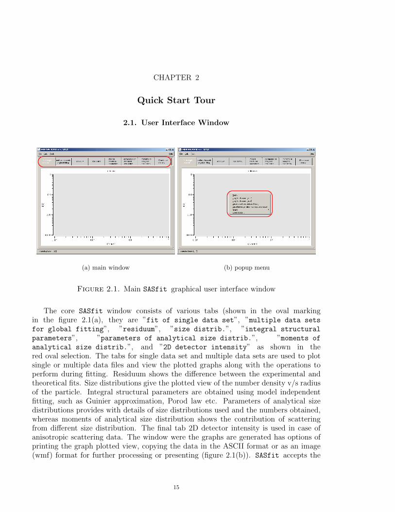
Figure 2.1. Main SASfit graphical user interface window
The core SASfit window consists of various tabs (shown in the oval markingin the figure 2.1(a), they are ”fit of single data set”, ”multiple data sets
for global fitting”, ”residuum”, ”size distrib.”, ”integral structural
parameters”, ”parameters of analytical size distrib.”, ”moments of
analytical size distrib.”, and ”2D detector intensity” as shown in thered oval selection. The tabs for single data set and multiple data sets are used to plotsingle or multiple data files and view the plotted graphs along with the operations toperform during fitting. Residuum shows the difference between the experimental andtheoretical fits. Size distributions give the plotted view of the number density v/s radiusof the particle. Integral structural parameters are obtained using model independentfitting, such as Guinier approximation, Porod law etc. Parameters of analytical sizedistributions provides with details of size distributions used and the numbers obtained,whereas moments of analytical size distribution shows the contribution of scatteringfrom different size distribution. The final tab 2D detector intensity is used in case ofanisotropic scattering data. The window were the graphs are generated has options ofprinting the graph plotted view, copying the data in the ASCII format or as an image(wmf) format for further processing or presenting (figure 2.1(b)). SASfit accepts the
15
16 2. QUICK START TOUR
isotropic data in the ASCII format. The data can be imported as a single data set orfor multiple data sets (several scattering curves).
2.2. Importing data files for a single data set
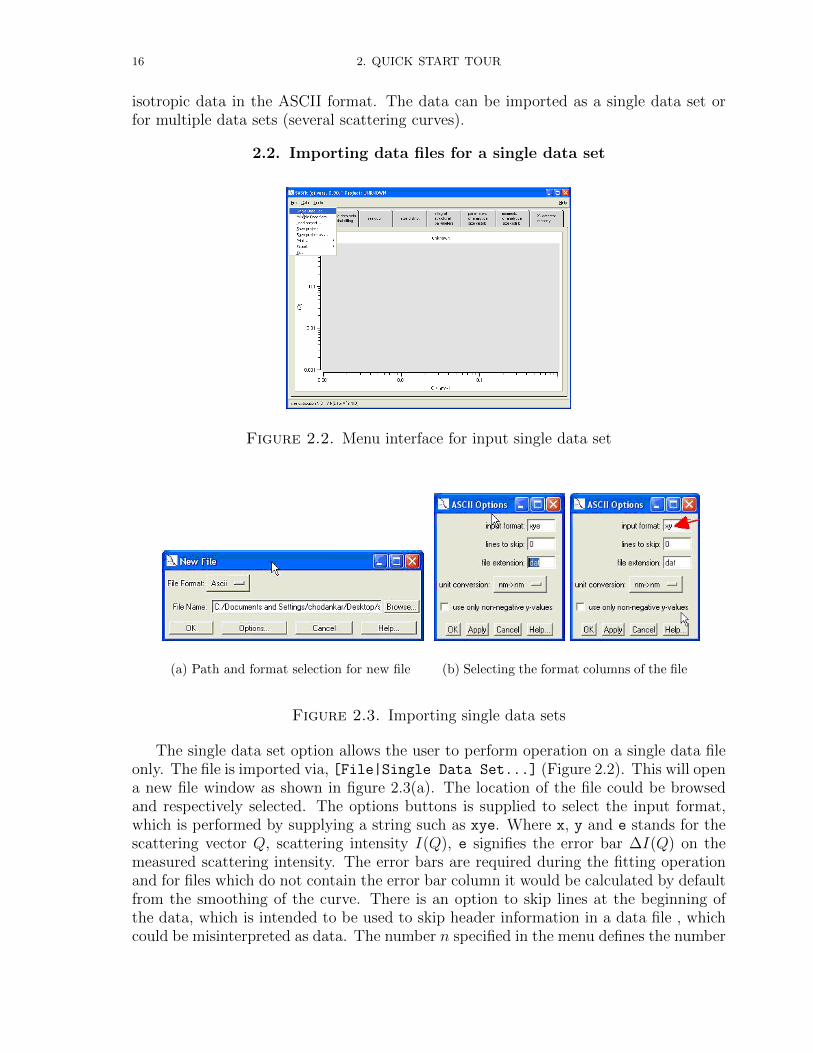
Figure 2.2. Menu interface for input single data set
(a) Path and format selection for new file (b) Selecting the format columns of the file
Figure 2.3. Importing single data sets
The single data set option allows the user to perform operation on a single data fileonly. The file is imported via, [File|Single Data Set...] (Figure 2.2). This will opena new file window as shown in figure 2.3(a). The location of the file could be browsedand respectively selected. The options buttons is supplied to select the input format,which is performed by supplying a string such as xye. Where x, y and e stands for thescattering vector Q, scattering intensity I(Q), e signifies the error bar ∆I(Q) on themeasured scattering intensity. The error bars are required during the fitting operationand for files which do not contain the error bar column it would be calculated by defaultfrom the smoothing of the curve. There is an option to skip lines at the beginning ofthe data, which is intended to be used to skip header information in a data file , whichcould be misinterpreted as data. The number n specified in the menu defines the number

2.2. IMPORTING DATA FILES FOR A SINGLE DATA SET 17
of lines skipped at the beginning of the data file. Furthermore a file extension can beprovided, unit conversions can be performed as well as only non-negative y-values couldbe selected for plotting and performing further analysis. On pressing ok the data isloaded and the graph is plotted, with a new window labeled merge files being opened.
(a) Merge window for merging different Q scalesinto a single profile
(b) An example showing merged data files (c) resolution parameter in-terface
Figure 2.4. Merging many data files to one data set
In SAS, data can be collected at different collimator and sample to detector distancesto correspond for a wide Q scale. Thus for a single sample at a given condition there canbe more than one data files, to merge all of them together for completing the scatteringprofile, the above shown window comes into play. As shown in the merge files window,the new file could be browsed and selected; it has to be read using the read file button.The newly read file is listed below the first file, if it’s a wrong selection it could bedeleted back, also one can scale the different files measured at different Q windows,using the divisor column to have a continuous scattering profile. After scaling all thedata profiles into one single profile, the statistically bad and unwanted data points canbe removed by skipping the points at the beginning and at the end of the data files. Theresolution parameters can be provided by pressing the resolution button and the required
18 2. QUICK START TOUR
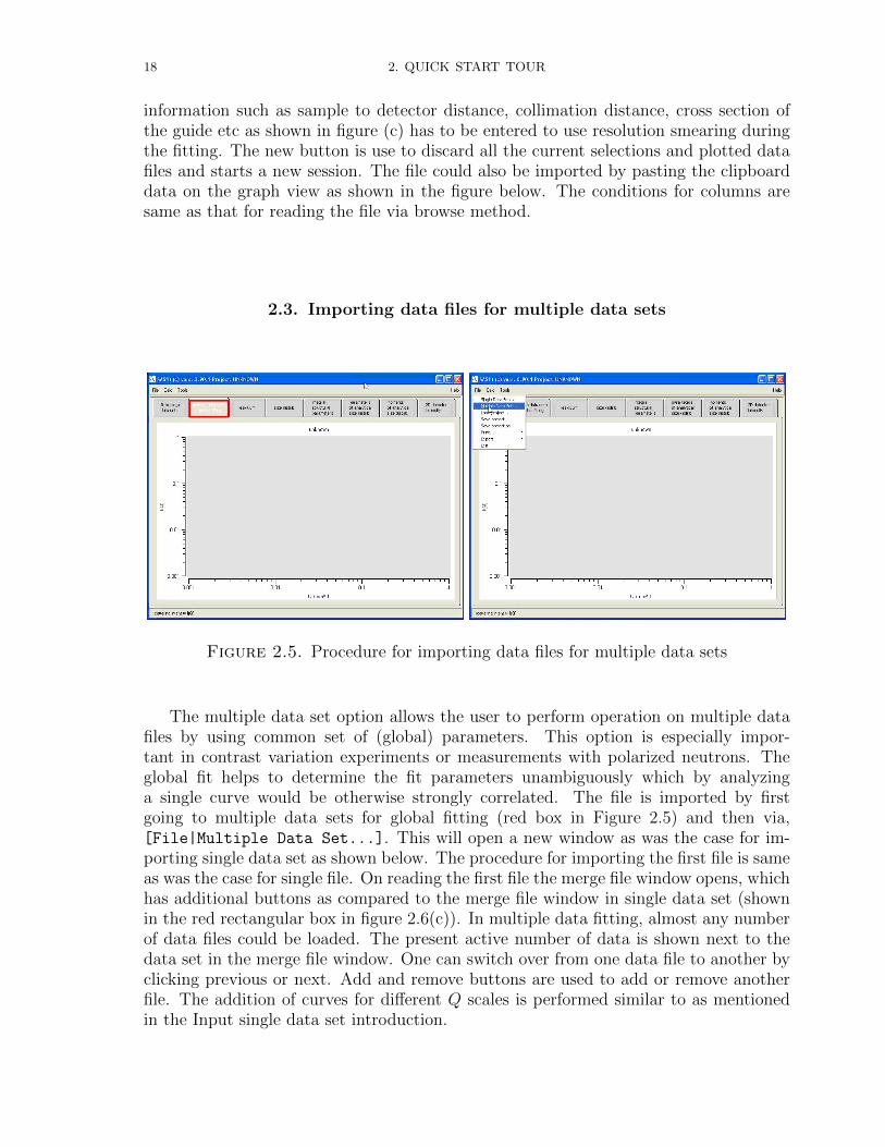
information such as sample to detector distance, collimation distance, cross section ofthe guide etc as shown in figure (c) has to be entered to use resolution smearing duringthe fitting. The new button is use to discard all the current selections and plotted datafiles and starts a new session. The file could also be imported by pasting the clipboarddata on the graph view as shown in the figure below. The conditions for columns aresame as that for reading the file via browse method.
2.3. Importing data files for multiple data sets
Figure 2.5. Procedure for importing data files for multiple data sets
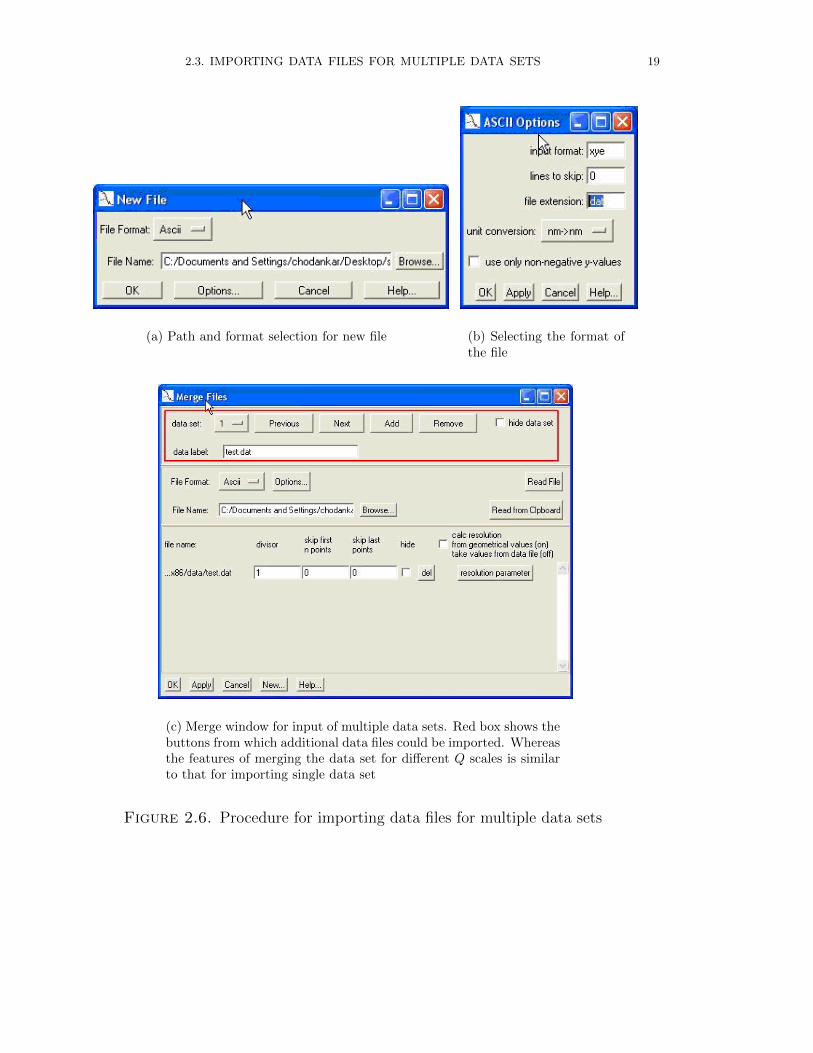
The multiple data set option allows the user to perform operation on multiple datafiles by using common set of (global) parameters. This option is especially impor-tant in contrast variation experiments or measurements with polarized neutrons. Theglobal fit helps to determine the fit parameters unambiguously which by analyzinga single curve would be otherwise strongly correlated. The file is imported by firstgoing to multiple data sets for global fitting (red box in Figure 2.5) and then via,[File|Multiple Data Set...]. This will open a new window as was the case for im-porting single data set as shown below. The procedure for importing the first file is sameas was the case for single file. On reading the first file the merge file window opens, whichhas additional buttons as compared to the merge file window in single data set (shownin the red rectangular box in figure 2.6(c)). In multiple data fitting, almost any numberof data files could be loaded. The present active number of data is shown next to thedata set in the merge file window. One can switch over from one data file to another byclicking previous or next. Add and remove buttons are used to add or remove anotherfile. The addition of curves for different Q scales is performed similar to as mentionedin the Input single data set introduction.
2.3. IMPORTING DATA FILES FOR MULTIPLE DATA SETS 19
(a) Path and format selection for new file (b) Selecting the format ofthe file
(c) Merge window for input of multiple data sets. Red box shows thebuttons from which additional data files could be imported. Whereasthe features of merging the data set for different Q scales is similarto that for importing single data set
Figure 2.6. Procedure for importing data files for multiple data sets

20 2. QUICK START TOUR
2.4. Simulating scattering curves
In addition to reading and loading data set, one can also have a realis-tic view of the experimental scattering data for a known structure by sim-ulating the scattering profile beforehand to get a feel of the actual experi-ment scattering profile. The simulation can be performed either for a sin-gle data set or for multiple data sets using global parameters. To gener-ate theoretical scattering profile, follow [Calc|Single Data Set...|simulate] or[Calc|Multiple Data Sets...|simulate], either of them to generate a single dataset or multiple data sets varied by changing the global parameter. The data can begenerated for vast number of form factors and structure factor included in the software.The simulation is calculated using physically relevant parameters, this is useful to planthe experiment and to know whether a given concentration and contrast would producea measurable signal.
(a) simulation of a single curve (b) simulation of multiple curves
Figure 2.7. Procedure for simulating data profiles for single as well asmultiple data files
2.5. Fitting
SASfit can analyse the data using both model-independent analysis and using anon-linear least square method to fit models. The model-independent analysis is apreliminary process of analyzing SAS data and does not require any advanced knowledgeof the system to extract structural information this includes fittings (Guinier, Kratky,Porod, power-laws, etc.). On the other hand in case of non-linear least square methodsa detailed fitting to the experimental data is performed using a wide variety of formfactors and structure factors. The SASfit model library consists of large number ofsuch functions, which can be readily used for the analysis. Moreover it can also fitdifferent size distributions.
2.5. FITTING 21
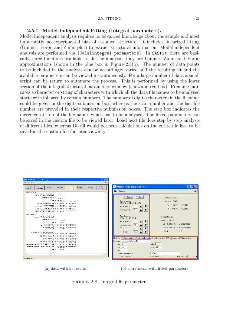
2.5.1. Model Independent Fitting (Integral parameters).Model independent analysis requires no advanced knowledge about the sample and mostimportantly no experimental bias of assumed structure. It includes linearized fitting(Guinier, Porod and Zimm plot) to extract structural information. Model independentanalysis are performed via [Cals|integral parameters]. In SASfit there are basi-cally three functions available to do the analysis; they are Guinier, Zimm and Porodapproximations (shown in the blue box in Figure 2.8(b). The number of data pointsto be included in the analysis can be accordingly varied and the resulting fit and theavailable parameters can be viewed instantaneously. For a large number of data a smallscript can be return to automate the process. This is performed by using the lowersection of the integral structural parameters window (shown in red box). Prename indi-cates a character or string of characters with which all the data file names to be analysedstarts with followed by certain numbers. The number of digits/characters in the filenamecould be given in the digits submission box, whereas the start number and the last filenumber are provided in their respective submission boxes. The step box indicates theincremental step of the file names which has to be analysed. The fitted parameters canbe saved in the custom file to be viewed later. Load next file does step by step analysisof different files, whereas Do all would perform calculations on the entire file list, to besaved in the custom file for later viewing.
(a) data with fit results (b) entry menu with fitted parameters
Figure 2.8. Integral fit parameters
22 2. QUICK START TOUR
A set of valuable size and integrated parameters that can be calculated directly fromthe scattering curves I(Q) [26, 128, 27, 147, 98, 50] consists of
Qinv =
∞∫0
Q2I(Q)dQ (scattering invariant) (2.1a)
S
V=
π
Qinv
limQ→∞
Q4I(Q)
(specific surface) (2.1b)
〈RG〉2 = 3
(− lim
Q→0
d[ln I(Q)]
d(Q2)
)(squared Guinier radius) (2.1c)
〈d〉 =4
π
∫∞0Q2I(Q)dQ
limQ→∞
Q4I(Q)
(average intersection length) (2.1d)
〈l〉 =π
Qinv
∞∫0
QI(Q)dQ (correlation length) (2.1e)
〈A〉 =2π
Qinv
∞∫0
I(Q)dQ (correlation surface) (2.1f)
〈V 〉 =2π2
Qinv
I(0) (correlation volume, Porod volume) (2.1g)
2.5.2. Model dependent analysis.2.5.2.1. Modeling a single data set.
For Modeling a SANS data set the SASfit -programm allows to describe experimentaldata with an arbitrary number of scattering objects types. Each of them can have a sizedistribution, whereby the user can choose over which parameter ai of the form factorthe integration will be performed. For example in case of a spherical shell with a coreradius of R and a shell thickness of ∆R SASfit allows to integrate either over the coreradius x = R or the shell thickness x = ∆R by marking the corresponding parameter(see option distr in Fig . 2.9(b)). Furthermore an additional structure factor can beincluded for each scattering object. Several ways to account for the structure factor havebeen implemented like the monodisperse approximation (4.1.1), decoupling approach(4.1.2), local monodisperse approximation (4.1.3), partial structure factor (4.1.4) andscaling approximation of partial structure factors (4.1.5). The details are described inchapter 4.
Implemented size distributions, form factors and structure factors are described inchapters 3, 4 and 6. Optional an additional smearing of this function with the instrumentresolution function Rav (Q, 〈Q〉) can be activated so that
I(〈Q〉) =
∞∫0
Rav (Q, 〈Q〉) dσdΩ
(Q) dQ (2.2)
A user interface shown in Fig. 2.9 is supplied to choose between the number ofscattering objects and to define parameter for each of them. Next to varying the different

2.5. FITTING 23
(a) Menu through which fitting procedure is ini-tiated
(b) User interface for fitting, containing differ-ent form factors and structure factor
(c) Tab summarizing the analyzed parameters
Figure 2.9. Menus for fitting a single data set
parameters one can mark those, which one would like to fix or to vary in a fittingprocedure (see option fit in Fig. ??(b)) Model dependent analysis for single files areperformed via [Calc|Single Data Set|Fit...].
2.5.2.2. Modeling multiple data sets.The multiple data set option allows the user to perform operation on multiple data
file by using common set (global) parameters. This option is especially important incontrast variation experiments or measurements with polarized neutrons. The global
24 2. QUICK START TOUR
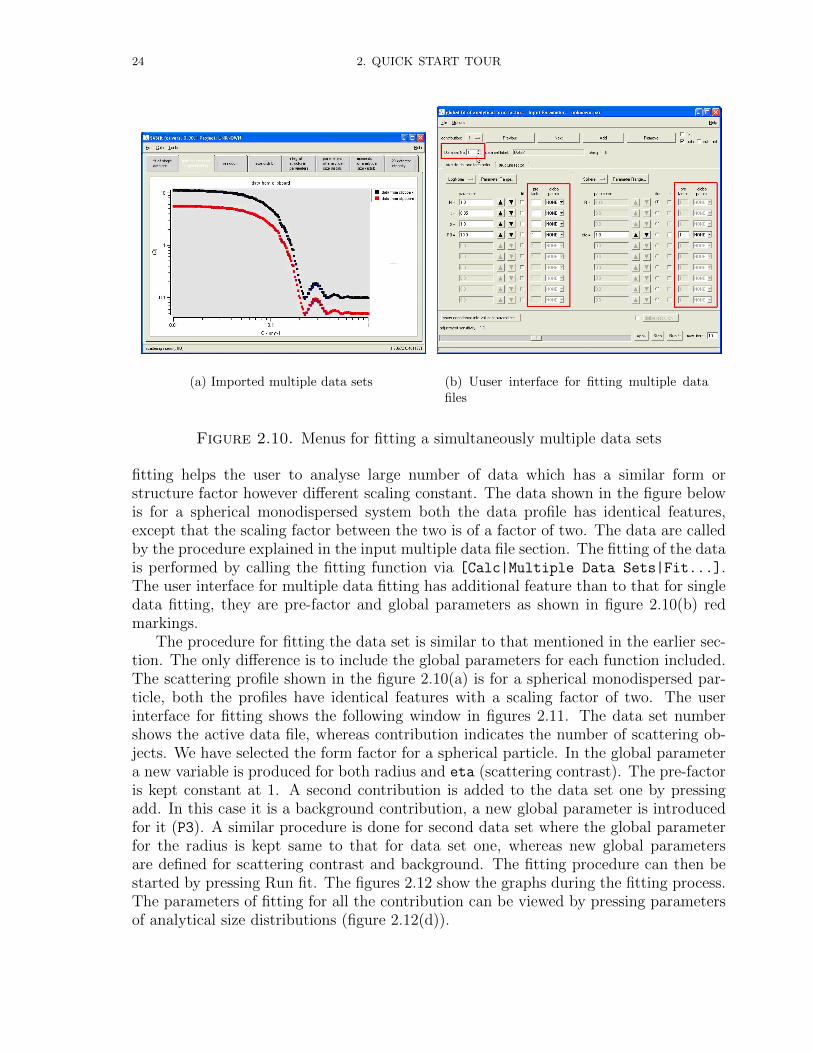
(a) Imported multiple data sets (b) Uuser interface for fitting multiple datafiles
Figure 2.10. Menus for fitting a simultaneously multiple data sets
fitting helps the user to analyse large number of data which has a similar form orstructure factor however different scaling constant. The data shown in the figure belowis for a spherical monodispersed system both the data profile has identical features,except that the scaling factor between the two is of a factor of two. The data are calledby the procedure explained in the input multiple data file section. The fitting of the datais performed by calling the fitting function via [Calc|Multiple Data Sets|Fit...].The user interface for multiple data fitting has additional feature than to that for singledata fitting, they are pre-factor and global parameters as shown in figure 2.10(b) redmarkings.
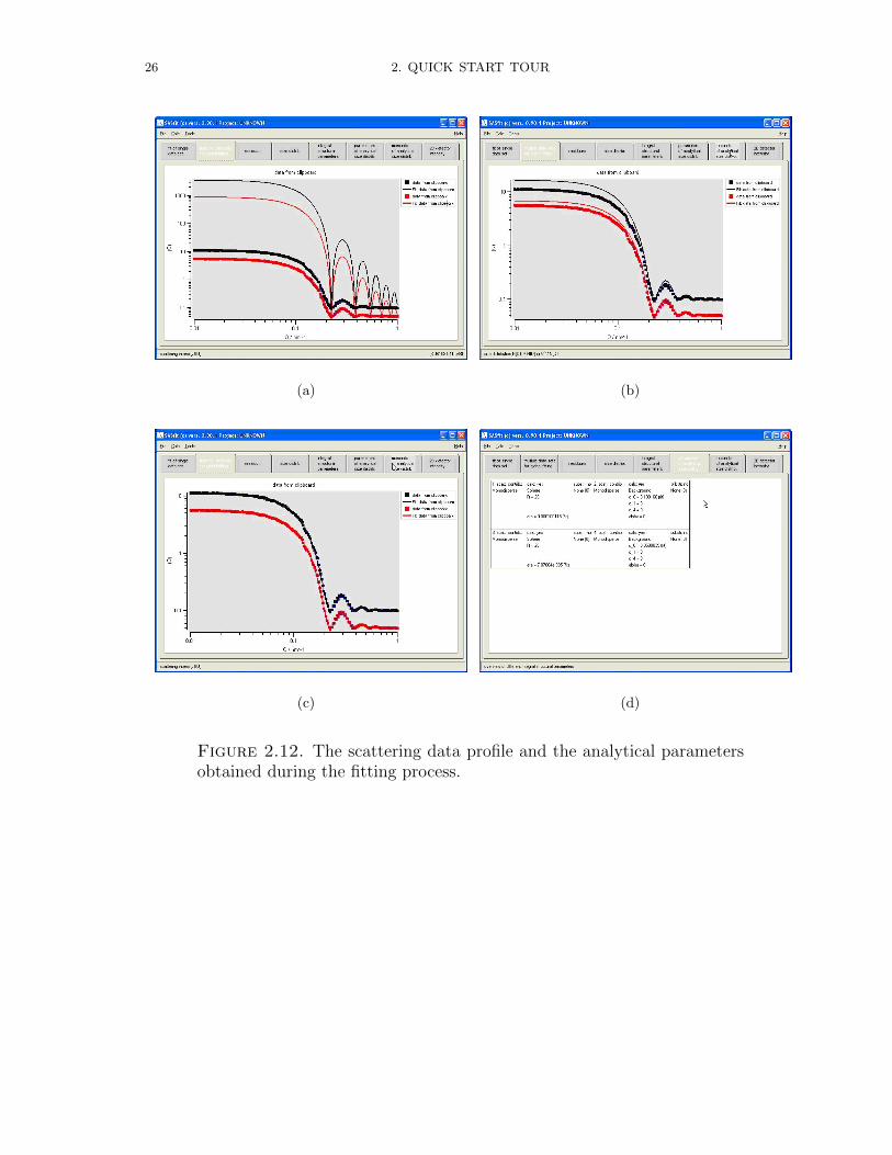
The procedure for fitting the data set is similar to that mentioned in the earlier sec-tion. The only difference is to include the global parameters for each function included.The scattering profile shown in the figure 2.10(a) is for a spherical monodispersed par-ticle, both the profiles have identical features with a scaling factor of two. The userinterface for fitting shows the following window in figures 2.11. The data set numbershows the active data file, whereas contribution indicates the number of scattering ob-jects. We have selected the form factor for a spherical particle. In the global parametera new variable is produced for both radius and eta (scattering contrast). The pre-factoris kept constant at 1. A second contribution is added to the data set one by pressingadd. In this case it is a background contribution, a new global parameter is introducedfor it (P3). A similar procedure is done for second data set where the global parameterfor the radius is kept same to that for data set one, whereas new global parametersare defined for scattering contrast and background. The fitting procedure can then bestarted by pressing Run fit. The figures 2.12 show the graphs during the fitting process.The parameters of fitting for all the contribution can be viewed by pressing parametersof analytical size distributions (figure 2.12(d)).

2.5. FITTING 25
(a) (b)
(c) (d)
Figure 2.11. Different windows showing different controlling parametersduring multiple data fitting.
26 2. QUICK START TOUR
(a) (b)
(c) (d)
Figure 2.12. The scattering data profile and the analytical parametersobtained during the fitting process.

2.6. FITTING STRATEGIES 27
2.6. Fitting strategies
28 2. QUICK START TOUR
2.7. Criteria for goodness-of-fit
All criteria shown below for testing the goodness of a fit should be considered withcaution [12, 118]. When you get data on a SAS instrument the the measured intensi-ties are measured with some statistical uncertainties. Normally one assumes Poissonstatistics to determine the uncertainty in the counting statistics. The data reductionsoftware should than perform a proper error propagation analysis for all succeedingdata treatment operations. However, by this procedure only statistical uncertaintiesare taken into account. All systematic uncertainties are than hopefully covered duringthe data treatment, as fir example background correction, transmission correction etc 13.
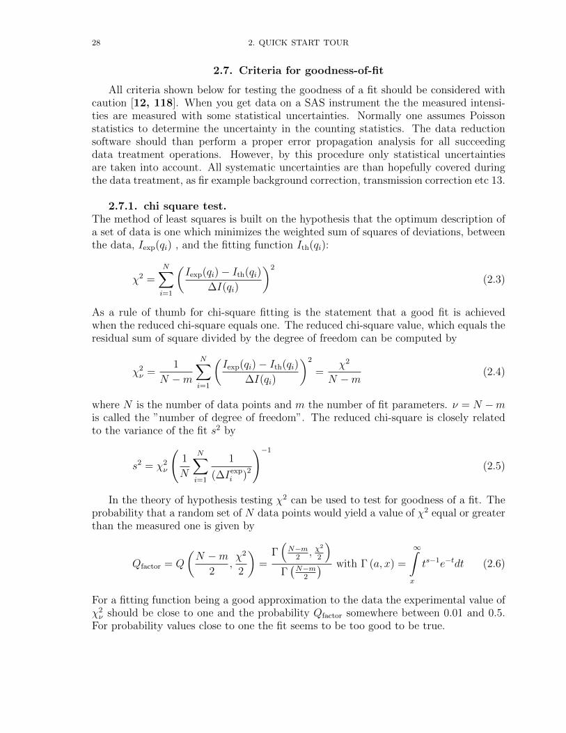
2.7.1. chi square test.The method of least squares is built on the hypothesis that the optimum description ofa set of data is one which minimizes the weighted sum of squares of deviations, betweenthe data, Iexp(qi) , and the fitting function Ith(qi):
χ2 =N∑i=1
(Iexp(qi)− Ith(qi)
∆I(qi)
)2
(2.3)
As a rule of thumb for chi-square fitting is the statement that a good fit is achievedwhen the reduced chi-square equals one. The reduced chi-square value, which equals theresidual sum of square divided by the degree of freedom can be computed by
χ2ν =
1
N −m
N∑i=1
(Iexp(qi)− Ith(qi)
∆I(qi)
)2
=χ2
N −m(2.4)
where N is the number of data points and m the number of fit parameters. ν = N −mis called the ”number of degree of freedom”. The reduced chi-square is closely relatedto the variance of the fit s2 by
s2 = χ2ν
(1
N
N∑i=1
1
(∆Iexpi )2
)−1
(2.5)
In the theory of hypothesis testing χ2 can be used to test for goodness of a fit. Theprobability that a random set of N data points would yield a value of χ2 equal or greaterthan the measured one is given by
Qfactor = Q
(N −m
2,χ2
2
)=
Γ(N−m
2, χ
2
2
)Γ(N−m
2
) with Γ (a, x) =
∞∫x
ts−1e−tdt (2.6)
For a fitting function being a good approximation to the data the experimental value ofχ2ν should be close to one and the probability Qfactor somewhere between 0.01 and 0.5.
For probability values close to one the fit seems to be too good to be true.
2.7. CRITERIA FOR GOODNESS-OF-FIT 29
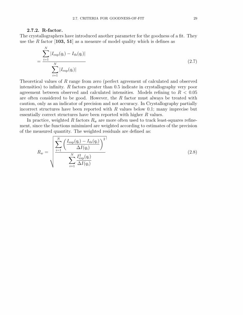
2.7.2. R-factor.The crystallographers have introduced another parameter for the goodness of a fit. Theyuse the R factor [103, 51] as a measure of model quality which is defines as
=
N∑i=1
|Iexp(qi)− Ith(qi)|
N∑i=1
|Iexp(qi)|(2.7)
Theoretical values of R range from zero (perfect agreement of calculated and observedintensities) to infinity. R factors greater than 0.5 indicate in crystallography very pooragreement between observed and calculated intensities. Models refining to R < 0.05are often considered to be good. However, the R factor must always be treated withcaution, only as an indicator of precision and not accuracy. In Crystallography partiallyincorrect structures have been reported with R values below 0.1; many imprecise butessentially correct structures have been reported with higher R values.
In practice, weighted R factors Rw are more often used to track least-squares refine-ment, since the functions minimized are weighted according to estimates of the precisionof the measured quantity. The weighted residuals are defined as:
Rw =
√√√√√√√√√N∑i=1
(Iexp(qi)− Ith(qi)
∆I(qi)
)2
N∑i=1
I2exp(qi)
∆I(qi)
(2.8)
30 2. QUICK START TOUR
2.8. Data I/O Formats
2.8.1. Input Format.
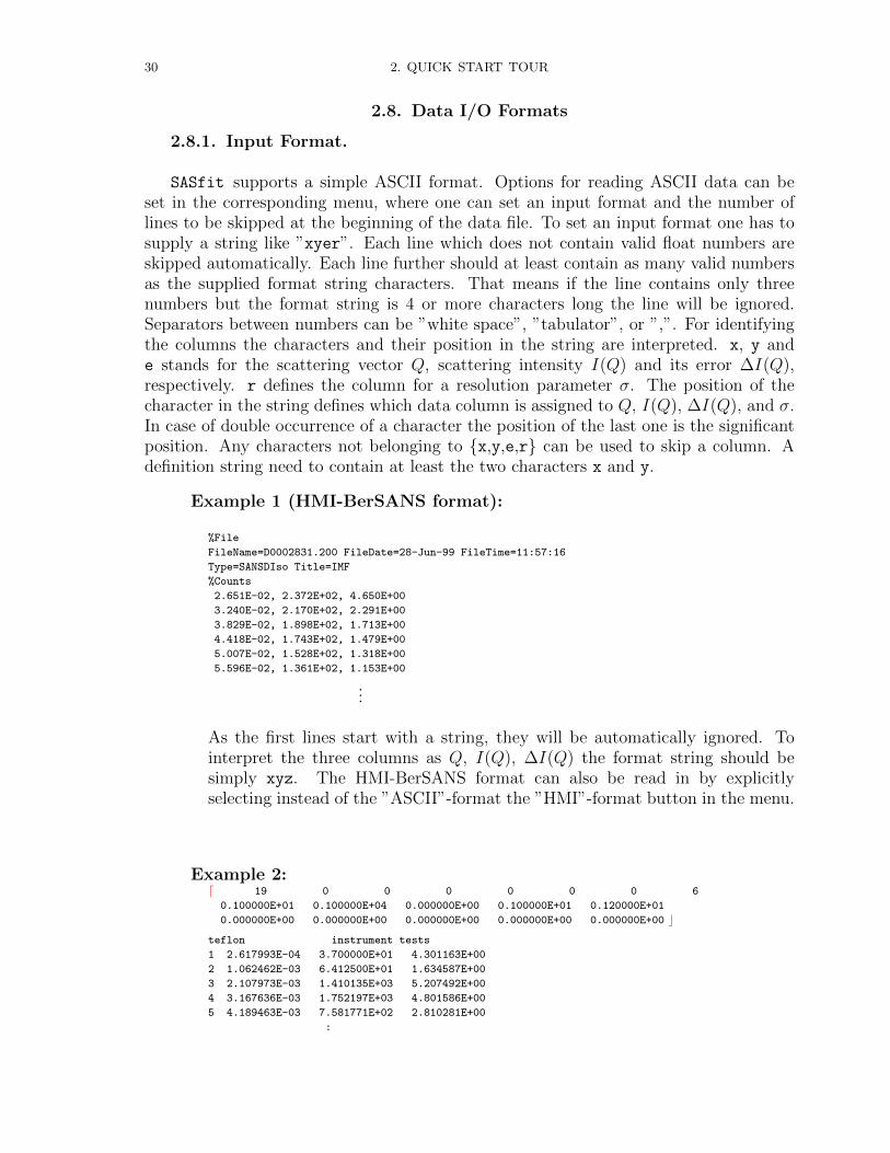
SASfit supports a simple ASCII format. Options for reading ASCII data can beset in the corresponding menu, where one can set an input format and the number oflines to be skipped at the beginning of the data file. To set an input format one has tosupply a string like ”xyer”. Each line which does not contain valid float numbers areskipped automatically. Each line further should at least contain as many valid numbersas the supplied format string characters. That means if the line contains only threenumbers but the format string is 4 or more characters long the line will be ignored.Separators between numbers can be ”white space”, ”tabulator”, or ”,”. For identifyingthe columns the characters and their position in the string are interpreted. x, y ande stands for the scattering vector Q, scattering intensity I(Q) and its error ∆I(Q),respectively. r defines the column for a resolution parameter σ. The position of thecharacter in the string defines which data column is assigned to Q, I(Q), ∆I(Q), and σ.In case of double occurrence of a character the position of the last one is the significantposition. Any characters not belonging to x,y,e,r can be used to skip a column. Adefinition string need to contain at least the two characters x and y.
Example 1 (HMI-BerSANS format):
%File
FileName=D0002831.200 FileDate=28-Jun-99 FileTime=11:57:16
Type=SANSDIso Title=IMF
%Counts
2.651E-02, 2.372E+02, 4.650E+00
3.240E-02, 2.170E+02, 2.291E+00
3.829E-02, 1.898E+02, 1.713E+00
4.418E-02, 1.743E+02, 1.479E+00
5.007E-02, 1.528E+02, 1.318E+00
5.596E-02, 1.361E+02, 1.153E+00
...
As the first lines start with a string, they will be automatically ignored. Tointerpret the three columns as Q, I(Q), ∆I(Q) the format string should besimply xyz. The HMI-BerSANS format can also be read in by explicitlyselecting instead of the ”ASCII”-format the ”HMI”-format button in the menu.
Example 2:d 19 0 0 0 0 0 0 6
0.100000E+01 0.100000E+04 0.000000E+00 0.100000E+01 0.120000E+01
0.000000E+00 0.000000E+00 0.000000E+00 0.000000E+00 0.000000E+00 c
teflon instrument tests
1 2.617993E-04 3.700000E+01 4.301163E+00
2 1.062462E-03 6.412500E+01 1.634587E+00
3 2.107973E-03 1.410135E+03 5.207492E+00
4 3.167636E-03 1.752197E+03 4.801586E+00
5 4.189463E-03 7.581771E+02 2.810281E+00
:
2.8. DATA I/O FORMATS 31
:
45 1.255376E-02 1.486688E+01 2.197023E-01
46 1.360724E-02 1.204012E+01 1.927716E-01
47 1.466810E-02 1.026648E+01 1.679423E-01
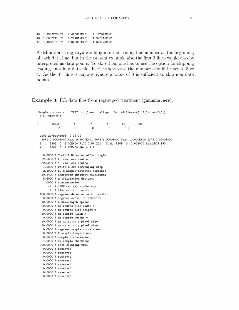
A definition string ixye would ignore the leading line number at the beginningof each data line, but in the present example also the first 3 lines would also beinterpreted as data points. To skip them one has to use the option for skippingleading lines in a data file. In the above case the number should be set to 3 or4. As the 4th line is anyway ignore a value of 3 is sufficient to skip non datapoints.
Example 3: ILL data files from regrouped treatment (gnnnnnn.eee).
Sample - d corrs TEST prot/deutr. ellipt. chs 44 lines+(Q, I(Q), errI(Q))
ILL SANS D11
d 8303 1 37 1 42 38
d 14 32 0 3 1 c
spol 20-Oct-1995 9:16:09
AvA1 0.0000E+00 AsA2 9.5000E-01 XvA3 1.0000E+00 XsA4 1.0000E+00 XfA5 0.0000E+00
S... 8303 0 1.00E+00 P100 0.5% 221 Sbak 8309 0 2.00E+00 Blank523 193
V... 8301 0 1.00E+00 Hhaps 911
0.0000 ! Theta-0 Detector offset angle
32.5000 ! X0 cms Beam centre
32.5000 ! Y0 cms Beam centre
1.0000 ! Delta-R cms regrouping step
2.5000 ! SD m Sample-detector distance
10.5400 ! Angstroms incident wavelength
5.6000 ! m collimation distance
1.0000 ! concentration
-3. ! ISUM central window sum
1. ! flux monitor counts
180.0000 ! degrees detector sector width
0.0000 ! degrees sector orientation
10.0000 ! % wavelength spread
20.0000 ! mm source slit width x
0.0000 ! mm source slit height y
10.0000 ! mm sample width x
0.0000 ! mm sample height y
10.0000 ! mm detector x pixel size
10.0000 ! mm detector y pixel size
0.0000 ! degrees sample normal/beam
0.0000 ! K sample temperature
0.0000 ! sample transmission
1.0000 ! mm sample thickness
900.0000 ! secs counting time
0.0000 ! reserved
0.0000 ! reserved
0.0000 ! reserved
0.0000 ! reserved
0.0000 ! reserved
0.0000 ! reserved
0.0000 ! reserved
0.0000 ! reserved
32 2. QUICK START TOUR
d 37 0 0 0 0 0 0 6
d 0.100000E+01 0.250000E+03 0.000000E+00 0.100000E+01 0.105400E+01
d 0.000000E+00 0.000000E+00 0.000000E+00 0.000000E+00 0.000000E+00
d 0.000000E+00 0.000000E+00 0.000000E+00 c2.194656E-03 3.442688E-01 8.329221E-02
5.466116E-03 3.000000E-01 5.008947E-02
8.480323E-03 3.877941E-01 4.232426E-02
1.189216E-02 6.498784E-01 1.519078E-02
1.497785E-02 7.493181E-01 1.173622E-02
...
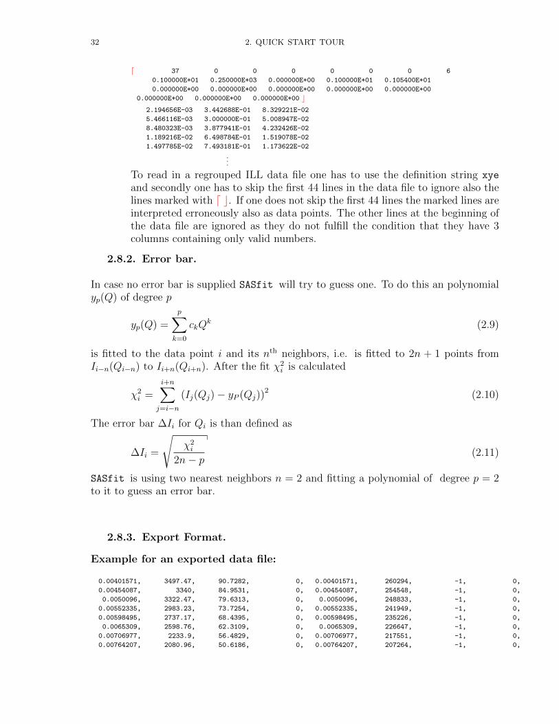
To read in a regrouped ILL data file one has to use the definition string xye
and secondly one has to skip the first 44 lines in the data file to ignore also thelines marked with d c. If one does not skip the first 44 lines the marked lines areinterpreted erroneously also as data points. The other lines at the beginning ofthe data file are ignored as they do not fulfill the condition that they have 3columns containing only valid numbers.
2.8.2. Error bar.
In case no error bar is supplied SASfit will try to guess one. To do this an polynomialyp(Q) of degree p
yp(Q) =
p∑k=0
ckQk (2.9)
is fitted to the data point i and its nth neighbors, i.e. is fitted to 2n + 1 points fromIi−n(Qi−n) to Ii+n(Qi+n). After the fit χ2
i is calculated
χ2i =
i+n∑j=i−n
(Ij(Qj)− yP (Qj))2 (2.10)
The error bar ∆Ii for Qi is than defined as
∆Ii =
√χ2i
2n− p(2.11)
SASfit is using two nearest neighbors n = 2 and fitting a polynomial of degree p = 2to it to guess an error bar.
2.8.3. Export Format.
Example for an exported data file:
0.00401571, 3497.47, 90.7282, 0, 0.00401571, 260294, -1, 0,
0.00454087, 3340, 84.9531, 0, 0.00454087, 254548, -1, 0,
0.0050096, 3322.47, 79.6313, 0, 0.0050096, 248833, -1, 0,
0.00552335, 2983.23, 73.7254, 0, 0.00552335, 241949, -1, 0,
0.00598495, 2737.17, 68.4395, 0, 0.00598495, 235226, -1, 0,
0.0065309, 2598.76, 62.3109, 0, 0.0065309, 226647, -1, 0,
0.00706977, 2233.9, 56.4829, 0, 0.00706977, 217551, -1, 0,
0.00764207, 2080.96, 50.6186, 0, 0.00764207, 207264, -1, 0,
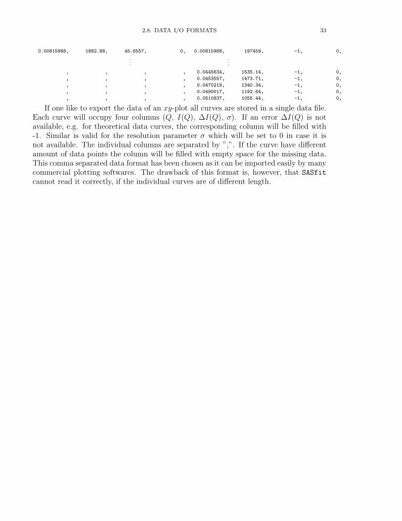
2.8. DATA I/O FORMATS 33
0.00815988, 1882.88, 45.6557, 0, 0.00815988, 197459, -1, 0,
......
, , , , 0.0445634, 1535.14, -1, 0,
, , , , 0.0453557, 1473.71, -1, 0,
, , , , 0.0470219, 1340.34, -1, 0,
, , , , 0.0490017, 1192.64, -1, 0,
, , , , 0.0510837, 1055.44, -1, 0,
If one like to export the data of an xy-plot all curves are stored in a single data file.Each curve will occupy four columns (Q, I(Q), ∆I(Q), σ). If an error ∆I(Q) is notavailable, e.g. for theoretical data curves, the corresponding column will be filled with-1. Similar is valid for the resolution parameter σ which will be set to 0 in case it isnot available. The individual columns are separated by ”,”. If the curve have differentamount of data points the column will be filled with empty space for the missing data.This comma separated data format has been chosen as it can be imported easily by manycommercial plotting softwares. The drawback of this format is, however, that SASfit
cannot read it correctly, if the individual curves are of different length.
34 2. QUICK START TOUR
2.9. Scattering length density calculator
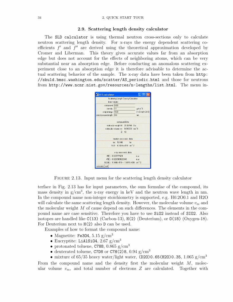
The SLD calculator is using thermal neutron cross-sections only to calculateneutron scattering length density. For x-rays the energy dependent scattering co-efficients f ′ and f ′′ are derived using the theoretical approximation developed byCromer and Liberman. This theory gives accurate values far from an absorptionedge but does not account for the effects of neighboring atoms, which can be verysubstantial near an absorption edge. Before conducting an anomalous scattering ex-periment close to an absorption edge it is therefore advisable to determine the ac-tual scattering behavior of the sample. The x-ray data have been taken from http:
//skuld.bmsc.washington.edu/scatter/AS_periodic.html and those for neutronsfrom http://www.ncnr.nist.gov/resources/n-lengths/list.html. The menu in-
Figure 2.13. Input menu for the scattering length density calculator
terface in Fig. 2.13 has for input parameters, the sum formulae of the compound, itsmass density in g/cm3, the x-ray energy in keV and the neutron wave length in nm.In the compound name non-integer stoichiometry is supported, e.g. H0.2O0.1 and H2Owill calculate the same scattering length density. However, the molecular volume vm andthe molecular weight M of cause depend on such differences. The elements in the com-pound name are case sensitive. Therefore you have to use SiO2 instead of SIO2. Alsoisotopes are handled like C(13) (Carbon-13), H(2) (Deuterium), or O(18) (Oxygen-18).For Deuterium next to H(2) also D can be used.
Examples of how to format the compound name:
• Magnetite: Fe3O4, 5.15 g/cm3
• Eucryptite: LiAlSiO4, 2.67 g/cm3
• protonated toluene, C7H8, 0.865 g/cm3
• deuterated toluene, C7D8 or C7H(2)8, 0.94 g/cm3
• mixture of 65/35 heavy water/light water, (D2O)0.65(H2O)0.35, 1.065 g/cm3
From the compound name and the density first the molecular weight M , molec-ular volume vm, and total number of electrons Z are calculated. Together with
2.9. SCATTERING LENGTH DENSITY CALCULATOR 35
the tabulated neutron scattering length and tabulated energy dependent scatteringcoefficient f ′(E) and f ′′(E) the corresponding coherent neutron scattering lengthbc =
∑i bi, coherent neutron scattering length density ηn,SLD = bc/vm and for x-
rays the complex energy dependent scattering scattering length density ηx,SLD =(Z − (Z/82.5)2.37 + f ′(E) + ıf ′′(E)) /vm of the compound are calculated.
36 2. QUICK START TOUR
2.10. Resolution Function [109]
〈k〉 = 2π/λ (2.12)
〈θ〉 = arcsin(〈Qav/(2〈k〉)) (2.13)
a1 =r1
L+ l/ cos2(2〈θ〉)(2.14)
a2 = r2 cos2(2〈θ〉)/l (2.15)
∆β1 =
a1 ≥ a2 :2r1
L− r2
2
2r1
cos4(2〈θ〉)l2L
(L+
l
cos2(2〈θ〉)
)2
a1 < a2 : 2r2
(1
L+
cos2(2〈θ〉)l
)− r2
1
2r2
l
L
× 1
cos2(2〈θ〉)(L+ l
cos2(2〈θ〉)
)(2.16)
σW = 〈Q〉∆λλ
1
2√
2 ln(2)(2.17)
σC1 = 〈k〉 cos(〈θ〉) ∆β1
2√
2 ln(2)(2.18)
σD1 = 〈k〉 cos(〈θ〉) cos2(2〈θ〉) D
l 2√
2 ln(2)(2.19)
σav = 〈k〉 cos(〈θ〉) cos2(2〈θ〉) ∆D
l 2√
2 ln(2)(2.20)
σ =√σ2W + σ2
C1 + σ2D1 + σ2
av (2.21)
Rav (Q, 〈Q〉) =Q
σ2exp
(−1
2
(Q2 + 〈Q〉2
)/σ2
)I0(Q〈Q〉/σ2) (2.22)
I(〈Q〉) =
∞∫0
Rav (Q, 〈Q〉) dσdΩ
(Q) dQ (2.23)
dσ
dΩ(Q) =
∞∫0
N(R)F 2(Q,R) dR (2.24)

CHAPTER 3
Form Factors
The different types of form factors are selected in the different submenus. Below onefinds how they are ordered. The definitions of the individual form factors are definedbelow. Under the submenu other functions all form factors under development andthose functions, which are not at all form factors but which have been implemented forsome other purposes are listed.
• Background• auxiliary and transition functions
– p(r) -> 4 pi r^2 sin(qr)/(qr)
– gamma(r) -> 4 pi sin(qr)/(qr)
• Spheres & Shells (3.1)– Sphere (3.1.1)– Spherical Shell i (3.1.2)– Spherical Shell ii (3.1.3)– Spherical Shell iii (3.1.4)– MultiLamellarVesicle (3.1.6)– RNDMultiLamellarVesicle
– RNDMultiLamellarVesicle2
– BiLayeredVesicle (3.1.5)– LinShell (8.3.2.1)– LinShell2 (8.3.2.2)– ExpShell (8.3.2.3)
• ellipsoidal obj. (3.2)– Ellipsoid i 3.2.2– Ellipsoid ii 3.2.1– EllipsoidalCoreShell 3.2.3– triaxEllShell1 3.2.4
• polymers & micelles (3.3)– polymer chains
∗ Gauss (3.3.1)∗ Gauss2 (3.3.1)∗ Gauss3 (3.3.1)∗ GaussPoly (3.3.1)∗ generalized Gaussian coil (3.3.1.5)∗ generalized Gaussian coil 2 (3.3.1.6)∗ generalized Gaussian coil 3 (3.3.1.7)
– polymer stars∗ BenoitStar (3.3.2)
37
38 3. FORM FACTORS
∗ PolydisperseStar (3.3.3)∗ Dozier (3.3.4.1)∗ Dozier2 (3.3.4.2)
– polymer rings∗ FlexibleRingPolymer (3.3.5)∗ mMemberedTwistedRing (3.3.6)∗ DaisyLikeRing (3.3.7)
– spherical & ellipsoidal micelles∗ SPHERE+Chains(RW) Nagg (3.3.11.2)∗ SPHERE+Chains(RW) Rc (3.3.11.2)∗ SPHERE+Chains(RW) (3.3.11.2)∗ SPHERE+Chains(SAW) Nagg
∗ SPHERE+Chains(SAW) Rc
∗ SPHERE+Chains(SAW)
∗ SPHERE+R^-a Nagg (3.3.11.8)∗ SPHERE+R^-a Rc (3.3.11.8)∗ SPHERE+R^-a (3.3.11.8)∗ SPHERE smooth interface+R^-a Nagg
∗ SPHERE smooth interface+R^-a Rc
∗ ELL+Chains(RW) Nagg (3.3.11.3)∗ ELL+Chains(RW) Rc (3.3.11.3)∗ ELL+Chains(RW) (3.3.11.3)∗ SphereWithGaussChains
∗ BlockCopolymerMicelle
– cylindrical & rod-like micelles∗ CYL+Chains(RW) Nagg (3.3.11.4)∗ CYL+Chains(RW) Rc (3.3.11.4)∗ CYL+Chains(RW) (3.3.11.4)∗ WORM+Chains(RW) nagg (3.3.11.5)∗ WORM+Chains(RW) Rc (3.3.11.5)∗ WORM+Chains(RW)(3.3.11.5)∗ ROD+Chains(RW) nagg (3.3.11.6)∗ ROD+Chains(RW) Rc (3.3.11.6)∗ ROD+Chains(RW) (3.3.11.6)∗ ROD+R^-a nagg (3.3.11.9)∗ ROD+R^-a Rc (3.3.11.9)∗ ROD+R^-a (3.3.11.9)∗ ROD+Exp nagg
∗ ROD+Exp Rc
∗ ROD+Exp
– local planar micelles (sheets, ULV)∗ DISC+Chains(RW) nagg
∗ DISC+Chains(RW) Lc
∗ DISC+Chains(RW)
∗ SphULV+Chains(RW) nagg
∗ SphULV+Chains(RW) tc
3. FORM FACTORS 39
∗ SphULV+Chains(RW)
∗ EllULV+Chains(RW) nagg
∗ EllULV+Chains(RW) tc
∗ EllULV+Chains(RW)
∗ CylULV+Chains(RW) nagg
∗ CylULV+Chains(RW) tc
∗ CylULV+Chains(RW)
– wormlike structures∗ WormLikeChainEXV (3.3.9)∗ KholodenkoWorm (3.3.10)
• cluster obj. (3.5)– Fisher-Burford (3.5.1)– MassFractExp(3.5.1)– MassFractGauss (3.5.1)– Aggregate (Exp(-x^a) Cut-Off) (3.5.1)– Aggregate (OverlapSph Cut-Off) (3.5.1)– DLCAggregation (3.5.1)– RLCAggregation (3.5.1)– MassFractOverlappingSph (3.5.1)– StackDiscs (3.5.2)– DumbbellShell (3.5.3)– two attached spheres
– DoubleShellChain (3.5.4)– TetrahedronDoubleShell (3.5.5)
• non-particular structures– OrnsteinZernike (3.4.4)– BroadPeak (3.4.5)– TeubnerStrey (3.4.1)– DAB (3.4.2)– Spinodal (3.4.3)– BeacaugeExpPowLaw (3.3.8)– BeacaugeExpPowLaw2 (3.3.8)– Guinier 3.4.6
• cylindrical obj. (3.6)– Disc (3.6.1)– Rod (3.6.2)– EllCylShell
– PorodCylinder (3.6.5)– LongCylinder (3.6.3)– FlatCylinder (3.6.4)– Cylinder (3.6.6)– LongCylShell (3.6.7)– CylShell1 (3.6.7)– CylShell2 (3.6.7)– ellCylShell1 (3.6.8)– ellCylShell2 (3.6.8)

40 3. FORM FACTORS
– alignedCylShell
– partly aligned CylShell
– Torus (3.6.11)– anisotropic obj.
∗ Pcs(Q) for planar obj.· Pcs:homogenousXS (3.7.2.1)· Pcs:TwoInfinitelyThinPlates (3.7.3)· Pcs:LayeredCentroSymmetricXS(3.7.4)· Pcs:BiLayerGauss (3.7.5)· Pcs:Plate+Chains(RW)
∗ Pcs(Q) for cylindrical obj.· Pcs:homogeneousXS· Pcs:CylindricalShell· Pcs:Rod+Chains(RW)· Pcs:ellCylSh
• plane obj.– homogenousXS (3.7.2.1)– SphSh+SD+homoXS
– EllSh+SD+homoXS
– EllSh+SD+homoXS(S)
– CylSh+SD+homoXS
– Disc+homoXS
– TwoInfinitelyThinPlates (3.7.3)– LayeredCentroSymmetricXS (3.7.4)– BiLayerGauss (3.7.5)
• sheared objects– ShearedCylinder (3.8.1)– ShearedCylGauss (3.8.3)
• magnetic objects (3.9)– MagneticShellPsi (3.9.1.3)– MagneticShellAniso (3.9.1.1)– MagneticShellCrossTerm (3.9.1.2)– SuperparamagneticFFpsi (3.9.2.1)– SuperparamagneticFFAniso (3.9.2.2)– SuperparamagneticFFIso (3.9.2.3)– SuperparamagneticFFCrossTerm (3.9.2.4)
• Mie FF for SLS (3.10)– MieSphere (3.10.1)– MieShell (3.10.2)
• Peaks (7)– Amplitude Functions
∗ Beta (Amplitude) (7.1.1)∗ Chi-squared (Amplitude) (7.2.1)∗ Erfc (Amplitude) (7.3.1∗ Error (Amplitude) (7.4.1)∗ exponentially modified Gaussian (Amplitude) (7.5.1)
3. FORM FACTORS 41
∗ Extreme Value (Amplitude) (7.6.1)∗ F-variance (Amplitude) (7.7.1)∗ Gamma (Amplitude) (7.8.1)∗ Gaussian (Amplitude) (7.9.1)∗ Gaussian-Lorentzian cross product (Amplitude) (7.10.1)∗ Gaussian-Lorentzian sum (Amplitude) (7.11.1)∗ generalized Gaussian 1 (Amplitude) (7.12.1)∗ generalized Gaussian 2 (Amplitude) (7.13.1)∗ Giddings (Amplitude) (7.14.1)∗ Inverted Gamma (Amplitude) (7.17.1)∗ Kumaraswamy (Amplitude) (7.18.1)∗ Laplace (Amplitude) (7.20.1)∗ Logistic (Amplitude) (7.21.1)∗ LogLogistic (Amplitude) (7.22.1)∗ LogNormal, 4 parameters (Amplitude) (7.23.2)∗ LogNormal (Amplitude) (7.24.1)∗ Lorentzian (Amplitude) (7.25.1)∗ Pearson IV (Amplitude) (7.27.1)∗ Pearson VII (Amplitude) (7.28.1)∗ pulse (Amplitude) (7.29.1)∗ pulse with 2nd width (Amplitude) (7.30.1)∗ pulse with power term (Amplitude) (7.31.1)∗ Student-t (Amplitude) (7.32.1)∗ Voigt (Amplitude) (7.33.1)∗ Weibull (Amplitude) (7.33.4)
– Area Functions∗ Beta (Area) (7.1.2)∗ Chi-squared (Area) (7.2.2)∗ Erfc (Area) (7.3.2∗ Error (Area) (7.4.2)∗ exponentially modified Gaussian (Area) (7.5.2)∗ Extreme Value (Area) (7.6.2)∗ F-variance (Area) (7.7.2)∗ Gamma (Area) (7.8.2)∗ Gaussian (Area) (7.9.2)∗ Gaussian-Lorentzian cross product (Area) (7.10.2)∗ Gaussian-Lorentzian sum (Area) (7.11.2)∗ generalized Gaussian 1 (Area) (7.12.2)∗ generalized Gaussian 2 (Area) (7.13.2)∗ Giddings (Area) (7.14.2)∗ Haarhoff - Van der Linde (Area) (7.15)∗ Half Gaussian Modified Gaussian (Area) (7.16)∗ Inverted Gamma (Area) (7.17.2)∗ Kumaraswamy (Area) (7.19)∗ Laplace (Area) (7.20.2)∗ Logistic (Area) (7.21.2)

42 3. FORM FACTORS
∗ LogNormal, 4 parameters (Area) (7.23.2)∗ LogNormal (Area) (7.24.2)∗ Lorentzian (Area) (7.25.2)∗ Pearson IV (Area) (7.27.2)∗ Pearson VII (Area) (7.28.2)∗ pulse (Area) (7.29.2)∗ pulse with 2nd width (Area) (7.30.2)∗ pulse with power term (Area) (7.31.2)∗ Student-t (Area) (7.32.2)∗ Voigt (Area) (7.33.2)∗ Weibull (Area) (7.33.5)
• other functions– Langevin– DoubleShell withSD– SuperparStroboPsi– SuperparStroboPsi2– SuperparStroboPsiSQ– SuperparStroboPsiBt1– SuperparStroboPsiLx– SuperparStroboPsiL2x– DLS Sphere RDG– Robertus1– JulichMicelle
3.1. SPHERES & SHELLS 43
3.1. Spheres & Shells
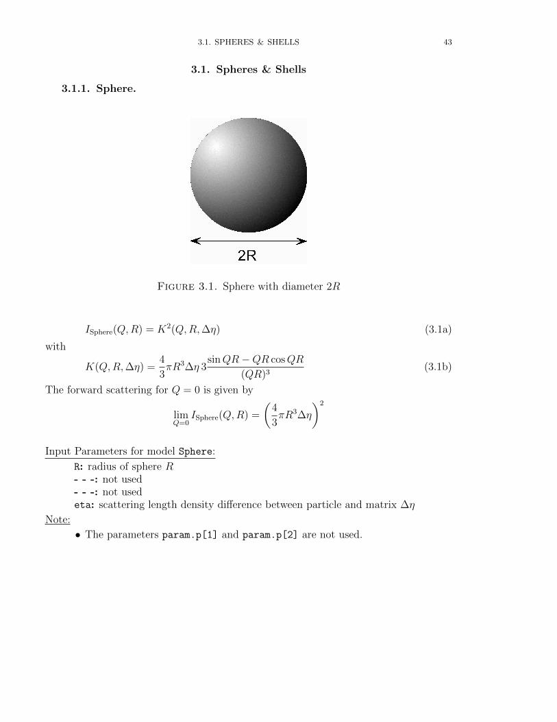
3.1.1. Sphere.
Figure 3.1. Sphere with diameter 2R
ISphere(Q,R) = K2(Q,R,∆η) (3.1a)
with
K(Q,R,∆η) =4
3πR3∆η 3
sinQR−QR cosQR
(QR)3(3.1b)
The forward scattering for Q = 0 is given by
limQ=0
ISphere(Q,R) =
(4
3πR3∆η
)2
Input Parameters for model Sphere:
R: radius of sphere R- - -: not used- - -: not usedeta: scattering length density difference between particle and matrix ∆η
Note:
• The parameters param.p[1] and param.p[2] are not used.
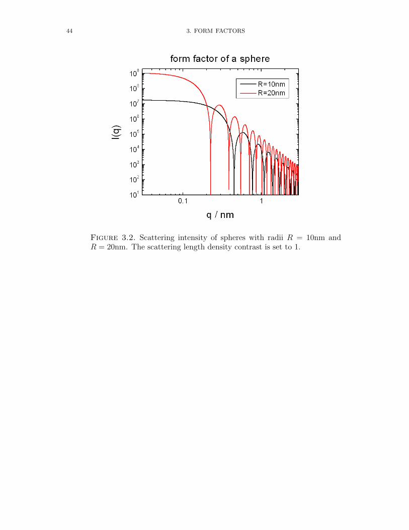
44 3. FORM FACTORS
Figure 3.2. Scattering intensity of spheres with radii R = 10nm andR = 20nm. The scattering length density contrast is set to 1.
3.1. SPHERES & SHELLS 45
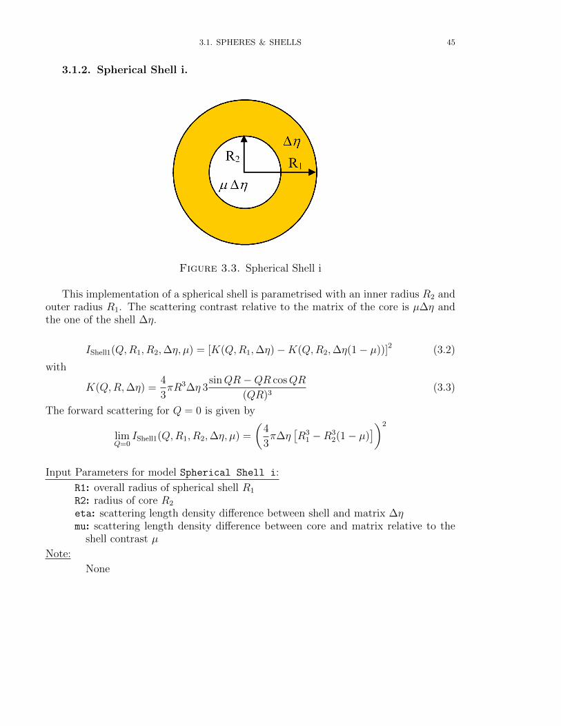
3.1.2. Spherical Shell i.
Figure 3.3. Spherical Shell i
This implementation of a spherical shell is parametrised with an inner radius R2 andouter radius R1. The scattering contrast relative to the matrix of the core is µ∆η andthe one of the shell ∆η.
IShell1(Q,R1, R2,∆η, µ) = [K(Q,R1,∆η)−K(Q,R2,∆η(1− µ))]2 (3.2)
with
K(Q,R,∆η) =4
3πR3∆η 3
sinQR−QR cosQR
(QR)3(3.3)
The forward scattering for Q = 0 is given by
limQ=0
IShell1(Q,R1, R2,∆η, µ) =
(4
3π∆η
[R3
1 −R32(1− µ)
])2
Input Parameters for model Spherical Shell i:
R1: overall radius of spherical shell R1
R2: radius of core R2
eta: scattering length density difference between shell and matrix ∆ηmu: scattering length density difference between core and matrix relative to the
shell contrast µ
Note:
None
46 3. FORM FACTORS
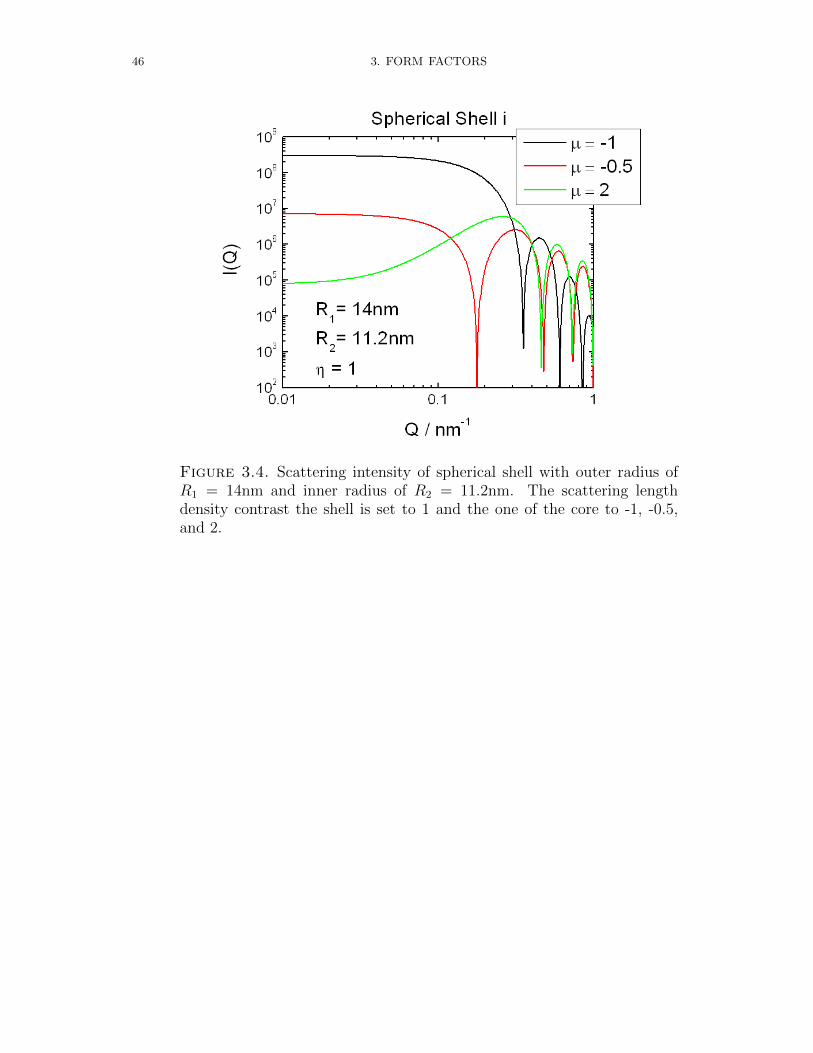
Figure 3.4. Scattering intensity of spherical shell with outer radius ofR1 = 14nm and inner radius of R2 = 11.2nm. The scattering lengthdensity contrast the shell is set to 1 and the one of the core to -1, -0.5,and 2.
3.1. SPHERES & SHELLS 47
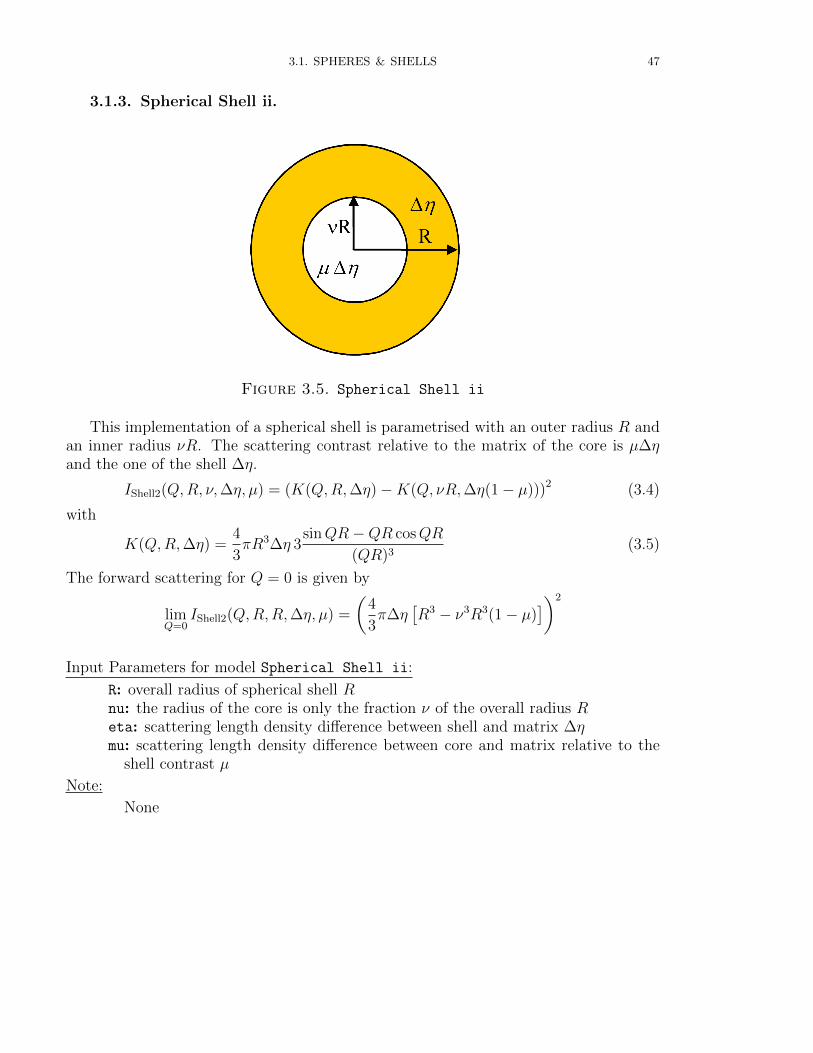
3.1.3. Spherical Shell ii.
Figure 3.5. Spherical Shell ii
This implementation of a spherical shell is parametrised with an outer radius R andan inner radius νR. The scattering contrast relative to the matrix of the core is µ∆ηand the one of the shell ∆η.
IShell2(Q,R, ν,∆η, µ) = (K(Q,R,∆η)−K(Q, νR,∆η(1− µ)))2 (3.4)
with
K(Q,R,∆η) =4
3πR3∆η 3
sinQR−QR cosQR
(QR)3(3.5)
The forward scattering for Q = 0 is given by
limQ=0
IShell2(Q,R,R,∆η, µ) =
(4
3π∆η
[R3 − ν3R3(1− µ)
])2
Input Parameters for model Spherical Shell ii:
R: overall radius of spherical shell Rnu: the radius of the core is only the fraction ν of the overall radius Reta: scattering length density difference between shell and matrix ∆ηmu: scattering length density difference between core and matrix relative to the
shell contrast µ
Note:
None
48 3. FORM FACTORS
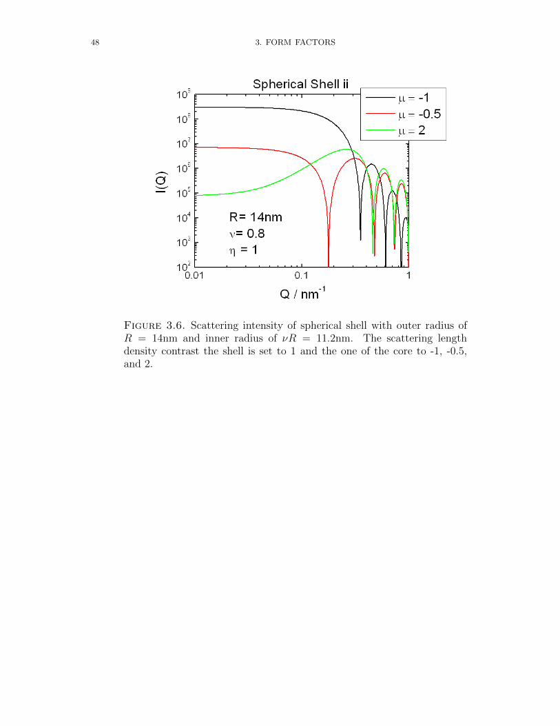
Figure 3.6. Scattering intensity of spherical shell with outer radius ofR = 14nm and inner radius of νR = 11.2nm. The scattering lengthdensity contrast the shell is set to 1 and the one of the core to -1, -0.5,and 2.

3.1. SPHERES & SHELLS 49
3.1.4. Spherical Shell iii.
Figure 3.7. Spherical Shell iii
This implementation of a spherical shell is parametrised with an inner radius R anda shell thickness ∆R. The scattering contrast relative to the matrix of the core is ∆η1
and the one of the shell ∆η2.
IShell3(Q,R,∆R,∆η1,∆η2) = [K(Q,R + ∆R,∆η2)−K(Q,R,∆η2 −∆η1)]2
(3.6)
with
K(Q,R,∆η) =4
3πR3∆η 3
sinQR−QR cosQR
(QR)3(3.7)
The forward scattering for Q = 0 is given by
limQ=0
IShell3(Q,R,∆R,∆η1,∆η2) =
(4
3π[(R + ∆R)3∆η2 −R3(∆η2 −∆η1)
])2
Input Parameters for model Spherical Shell iii:
R: radius of core RdR: thickness of the shell ∆Reta1: scattering length density difference between core and matrix ∆η1
eta2: scattering length density difference between shell and matrix ∆η2
Note:
None

50 3. FORM FACTORS
Figure 3.8. Scattering intensity of spherical shell with core radius ofR = 11.2nm and shell thickness of ∆R = 2.8nm. The scattering lengthdensity contrast the shell is set to 1 and the one of the core to -1, -0.5,and 2.

3.1. SPHERES & SHELLS 51
3.1.5. Bilayered Vesicle.
Figure 3.9. BiLayeredVesicle
IBLV(Q) =
(+K(Q,Rc, ηsol − ηt) +K(Q,Rc + tt, ηt − ηh) (3.8)
+K(Q,Rc + tt + th, ηh − ηt) +K(Q,Rc + 2tt + th, ηt − ηsol))2
with
K(Q,R,∆η) =4
3πR3∆η 3
sinQR−QR cosQR
(QR)3(3.9)
Input Parameters for model BilayeredVesicle:
R c: radius of core Rc which consists of solventt h: thickness of outer part of bilayer (in contact with solvent, head group) tht t: thickness of inner part of bilayer (tail group) tteta sol: scattering length density of solvent ηsol
eta h: scattering length density of outer part of bilayer ηh
eta t: scattering length density of inner part of bilayer ηt
Note:
None

52 3. FORM FACTORS
Figure 3.10. Scattering intensity of a bilayered vesicle. The scatter-ing intensity has been calculated with a lognormal [LogNorm(N = 1, σ=0.05, p=1, R=30)] size distribution for the vesicle radius Rc.
3.1. SPHERES & SHELLS 53
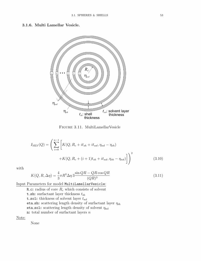
3.1.6. Multi Lamellar Vesicle.
Figure 3.11. MultiLamellarVesicle
IMLV(Q) =
(n−1∑i=0
[K(Q,Rc + itsh + itsol, ηsol − ηsh)
+K(Q,Rc + (i+ 1)tsh + itsol, ηsh − ηsol)])2
(3.10)
with
K(Q,R,∆η) =4
3πR3∆η 3
sinQR−QR cosQR
(QR)3(3.11)
Input Parameters for model MultiLamellarVesicle:
R c: radius of core Rc which consists of solventt sh: surfactant layer thickness tsht sol: thickness of solvent layer tsol
eta sh: scattering length density of surfactant layer ηsh
eta sol: scattering length density of solvent ηsol
n: total number of surfactant layers n
Note:
None
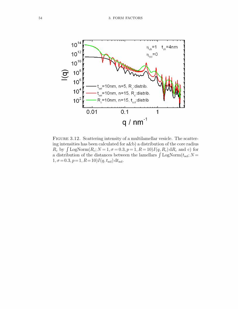
54 3. FORM FACTORS
Figure 3.12. Scattering intensity of a multilamellar vesicle. The scatter-ing intensities has been calculated for a&b) a distribution of the core radiusRc by
∫LogNorm(Rc;N = 1, σ= 0.3, p= 1, R= 10)I(q, Rc) dRc and c) for
a distribution of the distances between the lamellars∫
LogNorm(tsol;N=1, σ=0.3, p=1, R=10)I(q, tsol) dtsol.

3.1. SPHERES & SHELLS 55
3.1.7. RNDMultiLamellarVesicle.
Figure 3.13. randomMultiLamellarVesicle
IRndMLV(Q) = ∆η2
N∑i=1
F 2i (q, Ri, tsh,i)
+ ∆η2
N∑i<j
2Fi(q, Ri, tsh,i)Fj(q, Rj, tsh,j)sin qrijqrij
(3.12)
with
rij = |Ri −Rj| (3.13a)
Fi(q, Ri, tsol,i) = K(q, Ri + tsol,i,∆η)−K(q, Ri,∆η) (3.13b)
K(q, R,∆η) =4
3πR3∆η 3
sin qR− qR cos qR
(qR)3(3.13c)
R1 = ranlognormal (log(Rc), σRc) (3.14a)
∆Ri = rangaussian (σtsol) (3.14b)
Ri = Ri−1 + tsh,i−1 + ∆Ri (3.14c)
Ri = Ri randir,3Dranuniform ∆tsol (3.14d)
Input Parameters for model RNDMultiLamellarVesicle:
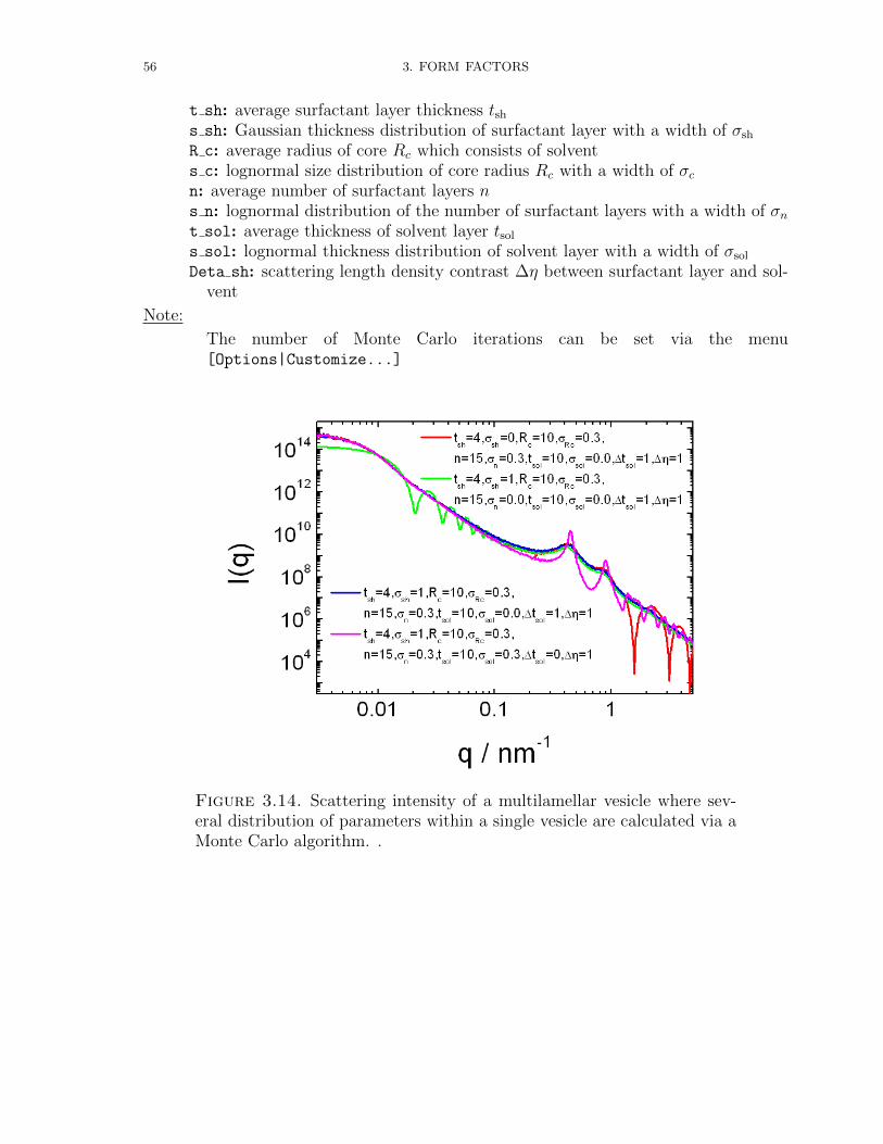
56 3. FORM FACTORS
t sh: average surfactant layer thickness tshs sh: Gaussian thickness distribution of surfactant layer with a width of σsh
R c: average radius of core Rc which consists of solvents c: lognormal size distribution of core radius Rc with a width of σcn: average number of surfactant layers ns n: lognormal distribution of the number of surfactant layers with a width of σnt sol: average thickness of solvent layer tsol
s sol: lognormal thickness distribution of solvent layer with a width of σsol
Deta sh: scattering length density contrast ∆η between surfactant layer and sol-vent
Note:
The number of Monte Carlo iterations can be set via the menu[Options|Customize...]
Figure 3.14. Scattering intensity of a multilamellar vesicle where sev-eral distribution of parameters within a single vesicle are calculated via aMonte Carlo algorithm. .
3.1. SPHERES & SHELLS 57
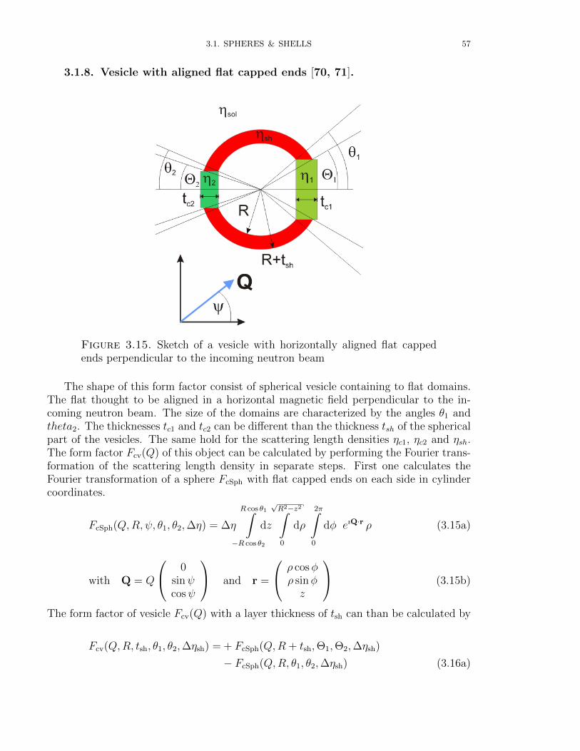
3.1.8. Vesicle with aligned flat capped ends [70, 71].
Figure 3.15. Sketch of a vesicle with horizontally aligned flat cappedends perpendicular to the incoming neutron beam
The shape of this form factor consist of spherical vesicle containing to flat domains.The flat thought to be aligned in a horizontal magnetic field perpendicular to the in-coming neutron beam. The size of the domains are characterized by the angles θ1 andtheta2. The thicknesses tc1 and tc2 can be different than the thickness tsh of the sphericalpart of the vesicles. The same hold for the scattering length densities ηc1, ηc2 and ηsh.The form factor Fcv(Q) of this object can be calculated by performing the Fourier trans-formation of the scattering length density in separate steps. First one calculates theFourier transformation of a sphere FcSph with flat capped ends on each side in cylindercoordinates.
FcSph(Q,R, ψ, θ1, θ2,∆η) = ∆η
R cos θ1∫−R cos θ2
dz
√R2−z2∫0
dρ
2π∫0
dφ eıQ·r ρ (3.15a)
with Q = Q
0sinψcosψ
and r =
ρ cosφρ sinφz
(3.15b)
The form factor of vesicle Fcv(Q) with a layer thickness of tsh can than be calculated by
Fcv(Q,R, tsh, θ1, θ2,∆ηsh) = + FcSph(Q,R + tsh,Θ1,Θ2,∆ηsh)
− FcSph(Q,R, θ1, θ2,∆ηsh) (3.16a)
58 3. FORM FACTORS
with
Θ1 = arcsin
(Rc1
R + tsh
), Rc1 = R sin (θ1) , (3.16b)
Θ2 = arcsin
(Rc2
R + tsh
), Rc2 = R sin (θ2) . (3.16c)
As the flat capped ends are allowed to have independent thicknesses tc1, tc2 and scatteringlength densities η1, η2 the scattering amplitude contribution of the flat capped ends,which have the shape of a disc, need to be corrected. Their contribution can be calculatedby
Fc(Q,R, θ1, θ2, . . . ) = Fc1(Q,R, θ1,∆ηc1)− Fd1(Q,R, td1,∆ηsh)
+ Fc2(Q,R, θ2,∆ηc2)− Fd2(Q,R, td2,∆ηsh)
= ∆ηc1
lc1+tc1∫lc1
dz
Rc1∫0
dρ
2π∫0
dφ eıQ·r ρ−∆ηsh
lc1+td1∫lc1
dz
Rc1∫0
dρ
2π∫0
dφ eıQ·r ρ
+ ∆ηc2
−lc2∫−(lc2+tc2)
dz
Rc2∫0
dρ
2π∫0
dφ eıQ·r ρ−∆ηsh
−lc2∫−(lc2+td2)
dz
Rc2∫0
dρ
2π∫0
dφ eıQ·r ρ
(3.17)
with
∆ηsh = ηsh − ηsol, ∆ηc1 = η1 − ηsol, ∆ηc2 = η2 − ηsol (3.18a)
lc1 = R cos θ1, lc2 = R cos θ2 (3.18b)
Rc1 = R sin θ1, Rc2 = R sin θ2 (3.18c)
td1 =
√(R + tsh)2 −R2
c1 −√R2 −R2
c1 (3.18d)
td2 =
√(R + tsh)2 −R2
c2 −√R2 −R2
c2 (3.18e)
(3.18f)
The solution of the integrals in eq. 3.15a and 3.17 are
FcSph(Q,R, ψ, θ1, θ2,∆η) = ∆η
R cos θ1∫−R cos θ2
dz
√R2−z2∫0
dρ
2π∫0
dφ eıQ·r ρ
∆η
R cos θ1∫−R cos θ2
dz exp (ıQz cosψ) 2π(R2 − z2
) J1
(Q√R2 − z2 sinψ
)Q√R2 − z2 sinψ
(3.19a)
3.1. SPHERES & SHELLS 59
and
Fci,di(Q,Rci,di , ψ,∆η) = ∆η
b∫a
dz
Rci∫0
dρ
2π∫0
dφ eıQ·r ρ
= 4πRı (exp (ıaQ cosψ)− exp (ıbQ cosψ)) J1 (QR sinψ)
sin (2ψ)Q2(3.19b)
whereby J1 the regular cylindrical Bessel function of first order. The overall scatteringintensity IalignedVes(Q,ψ, . . . ) is finally given by
IalignedVes(Q,ψ, . . . ) = |Fcv(Q,R, ψ, tsh, θ1, θ2,∆ηsh) + Fc(Q,R, ψ, θ1, θ2, . . . )|2
(3.20)
Input Parameters for the models of MagneticFieldAlignedVesicle:
Rsh: radius of spherical vesicle shelltheta1: angle to describe size of first capped sidetheta2: angle to describe size of second capped sidet sh: thickness of spherical vesicle shellt c1: thickness of first flat capped sidet c2: thickness of second flat capped sideeta sh: scattering length density of spherical vesicle shelleta 1: scattering length density of first capped sideeta 2: scattering length density of second capped sideeta sol: scattering length density of solvent
Note:
None
60 3. FORM FACTORS
3.2. Ellipsoidal Objects
3.2.1. Ellipsoid with two equal semi-axis R and semi-principal axes νR.
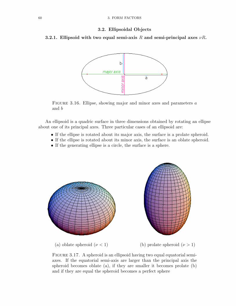
Figure 3.16. Ellipse, showing major and minor axes and parameters aand b
An ellipsoid is a quadric surface in three dimensions obtained by rotating an ellipseabout one of its principal axes. Three particular cases of an ellipsoid are:
• If the ellipse is rotated about its major axis, the surface is a prolate spheroid.• If the ellipse is rotated about its minor axis, the surface is an oblate spheroid.• If the generating ellipse is a circle, the surface is a sphere.
(a) oblate spheroid (ν < 1) (b) prolate spheroid (ν > 1)
Figure 3.17. A spheroid is an ellipsoid having two equal equatorial semi-axes. If the equatorial semi-axis are larger than the principal axis thespheroid becomes oblate (a), if they are smaller it becomes prolate (b)and if they are equal the spheroid becomes a perfect sphere
3.2. ELLIPSOIDAL OBJECTS 61
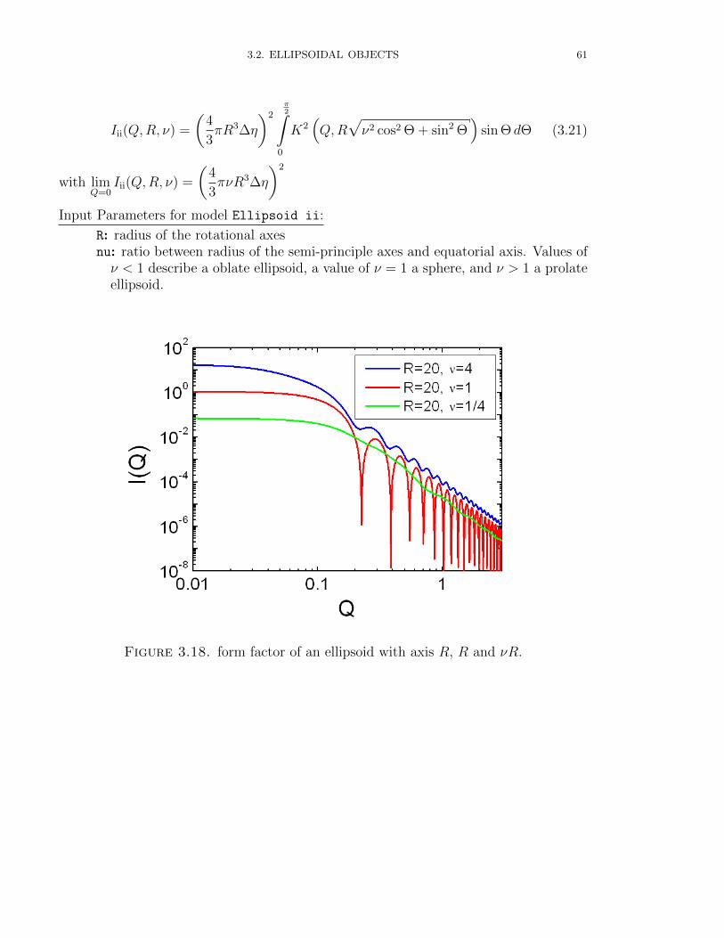
Iii(Q,R, ν) =
(4
3πR3∆η
)2π2∫
0
K2(Q,R
√ν2 cos2 Θ + sin2 Θ
)sin Θ dΘ (3.21)
with limQ=0
Iii(Q,R, ν) =
(4
3πνR3∆η
)2
Input Parameters for model Ellipsoid ii:
R: radius of the rotational axesnu: ratio between radius of the semi-principle axes and equatorial axis. Values ofν < 1 describe a oblate ellipsoid, a value of ν = 1 a sphere, and ν > 1 a prolateellipsoid.
Figure 3.18. form factor of an ellipsoid with axis R, R and νR.
62 3. FORM FACTORS
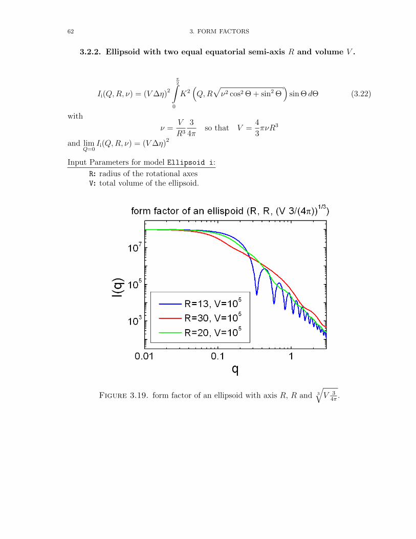
3.2.2. Ellipsoid with two equal equatorial semi-axis R and volume V .
Ii(Q,R, ν) = (V∆η)2
π2∫
0
K2(Q,R
√ν2 cos2 Θ + sin2 Θ
)sin Θ dΘ (3.22)
with
ν =V
R3
3
4πso that V =
4
3πνR3
and limQ=0
Ii(Q,R, ν) = (V∆η)2
Input Parameters for model Ellipsoid i:
R: radius of the rotational axesV: total volume of the ellipsoid.
Figure 3.19. form factor of an ellipsoid with axis R, R and 3
√V 3
4π.
3.2. ELLIPSOIDAL OBJECTS 63
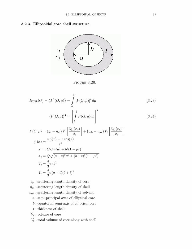
3.2.3. Ellipsoidal core shell structure.
Figure 3.20.
IECSh(Q) =⟨F 2(Q, µ)
⟩=
1∫0
[F (Q, µ)]2 dµ (3.23)
〈F (Q, µ)〉2 =
1∫0
F (Q, µ)dµ
2
(3.24)
F (Q, µ) = (ηc − ηsh)Vc
[3j1(xc)
xc
]+ (ηsh − ηsol)Vt
[3j1(xt)
xt
]j1(x) =
sin(x)− x cos(x)
x2
xc = Q√a2µ2 + b2(1− µ2)
xc = Q√
(a+ t)2µ2 + (b+ t)2(1− µ2)
Vc =4
3πab2
Vt =4
3π(a+ t)(b+ t)2
ηc : scattering length density of core
ηsh : scattering length density of shell
ηsol : scattering length density of solvent
a : semi-principal axes of elliptical core
b : equatorial semi-axis of elliptical core
t : thickness of shell
Vc : volume of core
Vt : total volume of core along with shell

64 3. FORM FACTORS
Input Parameters for model EllipsoidalCoreShell:
a: semi-principal axes of elliptical core ab: equatorial semi-axis axes of elliptical core bt: thickness of shell teta c: scattering length density of core ηc
eta sh: scattering length density of shell ηsh
eta sol: scattering length density of solvent ηsol
Figure 3.21. form factor of an ellipsoidal core shell a, b, b and t.
3.2. ELLIPSOIDAL OBJECTS 65
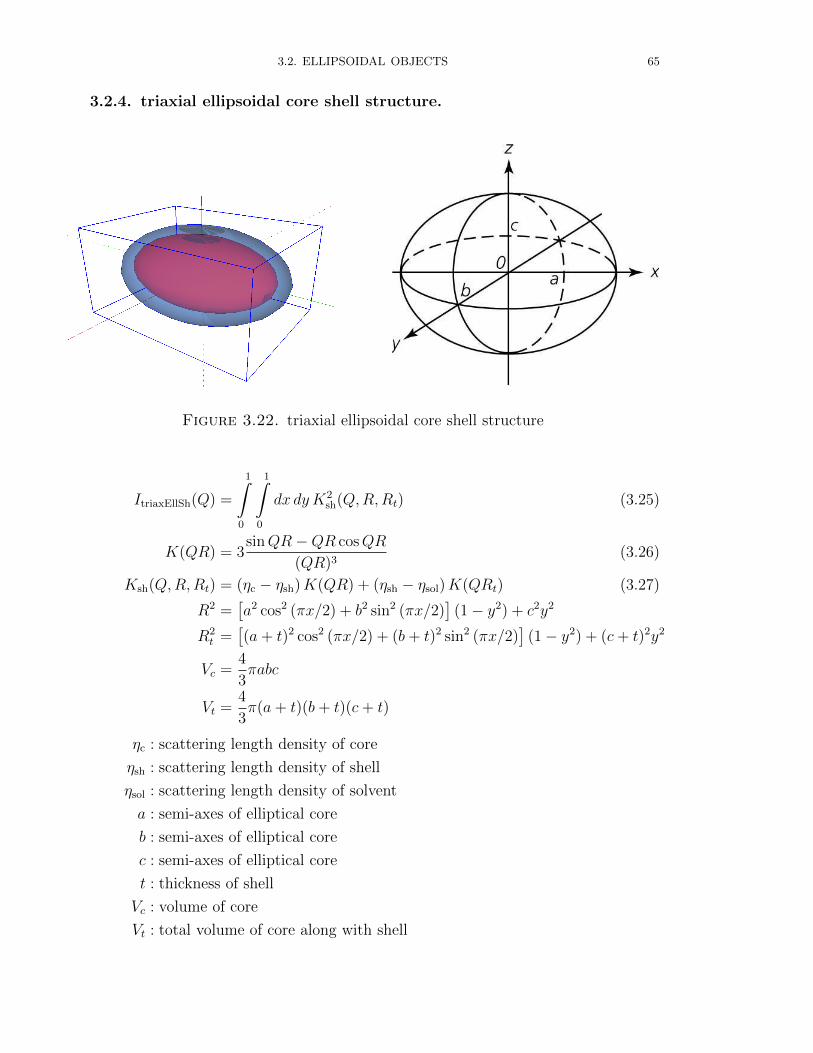
3.2.4. triaxial ellipsoidal core shell structure.
Figure 3.22. triaxial ellipsoidal core shell structure
ItriaxEllSh(Q) =
1∫0
1∫0
dx dy K2sh(Q,R,Rt) (3.25)
K(QR) = 3sinQR−QR cosQR
(QR)3(3.26)
Ksh(Q,R,Rt) = (ηc − ηsh)K(QR) + (ηsh − ηsol)K(QRt) (3.27)
R2 =[a2 cos2 (πx/2) + b2 sin2 (πx/2)
](1− y2) + c2y2
R2t =
[(a+ t)2 cos2 (πx/2) + (b+ t)2 sin2 (πx/2)
](1− y2) + (c+ t)2y2
Vc =4
3πabc
Vt =4
3π(a+ t)(b+ t)(c+ t)
ηc : scattering length density of core
ηsh : scattering length density of shell
ηsol : scattering length density of solvent
a : semi-axes of elliptical core
b : semi-axes of elliptical core
c : semi-axes of elliptical core
t : thickness of shell
Vc : volume of core
Vt : total volume of core along with shell
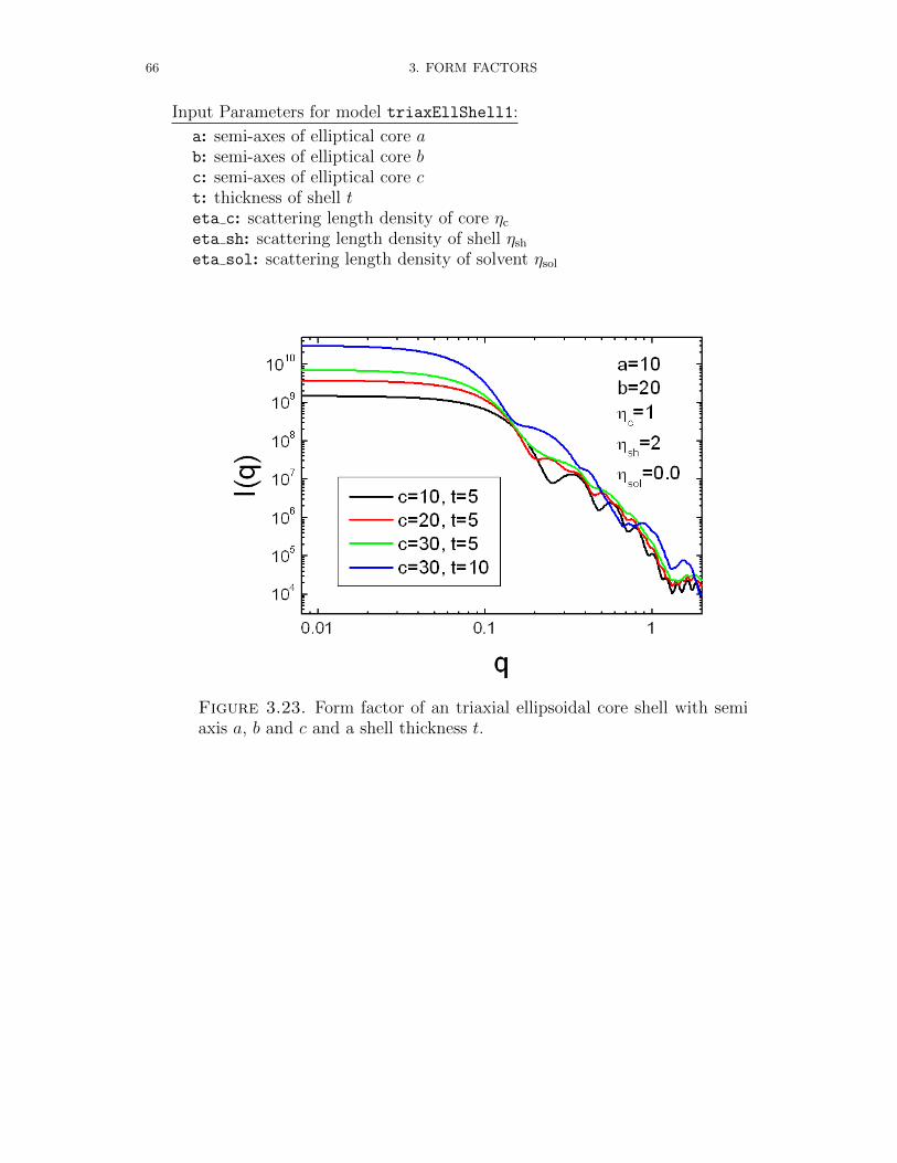
66 3. FORM FACTORS
Input Parameters for model triaxEllShell1:
a: semi-axes of elliptical core ab: semi-axes of elliptical core bc: semi-axes of elliptical core ct: thickness of shell teta c: scattering length density of core ηc
eta sh: scattering length density of shell ηsh
eta sol: scattering length density of solvent ηsol
Figure 3.23. Form factor of an triaxial ellipsoidal core shell with semiaxis a, b and c and a shell thickness t.
3.3. POLYMERS AND MICELLES 67
3.3. Polymers and Micelles
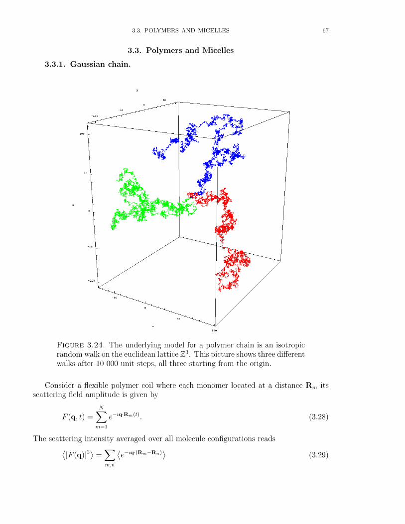
3.3.1. Gaussian chain.
Figure 3.24. The underlying model for a polymer chain is an isotropicrandom walk on the euclidean lattice Z3. This picture shows three differentwalks after 10 000 unit steps, all three starting from the origin.
Consider a flexible polymer coil where each monomer located at a distance Rm itsscattering field amplitude is given by
F (q, t) =N∑m=1
e−ıq·Rm(t). (3.28)
The scattering intensity averaged over all molecule configurations reads⟨|F (q)|2
⟩=∑m,n
⟨e−ıq·(Rm−Rn)
⟩(3.29)

68 3. FORM FACTORS
As the monomer segments Rm−Rn are Gaussian distributed the averages 〈· · · 〉 can bewritten as⟨
e−ıq·(Rm−Rn)⟩
= eq2
6 〈(Rm−Rn)2〉 (3.30a)
= e−q2b2
6|m−n|2ν (3.30b)
Here b is the statistical segment length and the contour length L equals L = Nb. Theaverage of the segment inter-distances squares is kept in the general form⟨
(Rm −Rn)2⟩ = b2|m− n|2ν . (3.31)
ν is the excluded volume parameter from the Flory mean field theory12 of polymersolutions. The radius of gyration RG is given by
R2G =
1
2N2
N∑m,n
⟨(Rm −Rn)2⟩ (3.32a)
=1
2N2
N∑m,n
b2|m− n|2ν (3.32b)
=b2
N
N∑k
(1− k
N
)k2ν (3.32c)
=b2
(2ν + 1) (2ν + 2)N2ν (3.32d)
Three cases are relevant:
(1) Self-avoiding walk corresponds to swollen chains with ν = 3/5, for which R2G =
25176b2N6/5.
(2) Pure random walk corresponds to chains in Θ-conditions (where solvent-solvent,monomer-monomer and solvent-monomer interactions are equivalent) with ν =1/2, for which R2
G = 16b2N .
(3) Self attracting walk corresponds to collapsed chains with ν = 1/3, for whichR2G = 9
40b2N2/3.
Using the general identity
N∑i,j
y(|i− j|) = N + 2N∑k=1
(N − k)y(k) (3.33)
the form factor reads
P (q) =1
N2|F (q)|2 =
1
N2
N + 2
N∑k=1
(N − k)e−q2b2
6k2ν
(3.34)
1P.J. Flory, ”Statistical Mechanics of Chain Molecules”, Interscience Publishers (1969)2Boualem Hammouda, the SANS toolbox.pdf
3.3. POLYMERS AND MICELLES 69
Going to the continuous limit (N 1), one obtains:
P (q) = 2
1∫0
dx (1− x)e−q2b2
6N2νx2ν
(3.35a)
=U
12ν Γ(
12ν
)− Γ
(1ν
)− U 1
2ν Γ(
12ν, U)
+ Γ(
1ν, U)
νU1/ν(3.35b)
with the modified variable
U =q2b2N2ν
6= (2ν + 1) (2ν + 2)
q2R2G
6(3.36)
and the unnormalized incomplete Gamma Function Γ(a, x) =∫∞x
dt ta−1 exp(−t) for a
real and x ≥ 0 and the Gamma function Γ(a) = Γ(a, 0) =∫∞
0dt ta−1 exp(−t). Polymer
chains follow Gaussian statistics in polymer solutions: they are swollen in good solventsν = 3/5, are thermally relaxed in ”theta”-solvents ν = 1/2 and partially precipitate inpoor solvents ν = 1/3. The familiar Debye function is recovered when ν = 1/2. Theasymptotic limit at large q-values of the generalized Gaussian chain is dominated by the
1
νU12ν
Γ(
12ν
)term which varies like U−1/(2ν) ∼ q−1/ν . For ν = 1 we get the limit of an
infinitesimal thin rod and for ν = 1/4 a compact object with a Porod law of q−4.SASfit has implemented the generalized form of a Gaussian (generalized
Gaussian coil) coil and the standard Debye formula Gauss. In both cases three versionare implemented which only differ in their parametrization of the forward scattering. Incase of the the Debye-formula also the polydisperse GaussPoly is implemented.
Gauss
3.3.1.1. Gauss [32].Flexible polymer chains which are not selfavoiding and obey Gaussian statistics. Debye(1947) has calculated the form factor of such chains:
IGauss(q) = I02exp(−u) + u− 1
u2(3.37)
u = q2R2g (3.38)
Input Parameters for model Gauss:
Rg: radius of gyration Rg
I0: forward scattering I0 for q = 0
Gauss
3.3.1.2. Gauss2 [32].This form factor differs only by the parametrization for the forward scattering I0 =

70 3. FORM FACTORS
(bp − V ηs)2 from the Debye formula in eq. 3.37
IGauss2(q) = β22exp(−u) + u− 1
u2(3.39)
u = q2R2g
β = bp − V ηs,
where bp is the scattering length of a polymer molecule of molecular volume V dissolvedin a solvent of scattering length density ηs from which the excess scattering length ofa polymer molecule β can be calculated. Combining this form factor with a Delta
size distribution 6.1 is needed to scale the scattering intensity. With proper values forthe form factor the parameter N of the Delta-distribution yields the particle numberdensity.
Input Parameters for model Gauss2:
Rg: radius of gyration Rg
b p: scattering length of polymer bp in [cm]V: molecular volume of a single polymer molecule V in [cm3]eta s: scattering length density of solvent ηs in [cm−1]
Gauss
3.3.1.3. Gauss3 [32].This form factor differs only by the parametrization for the forward scattering I0 =(bp − Mw
Naρpηs)
2 from the Debye formula in eq. 3.37
IGauss3(q) = β22exp(−u) + u− 1
u2(3.40)
with
u = q2R2g
β = bp − V ηs
V =Mw
NaρpNa = Avogadro number
Input Parameters for model Gauss3:
Rg: radius of gyration Rg
b p: scattering length of polymer bp in [cm]M w: molecular weight of polymer Mw in [g/mol]rho p: mass density of polymer ρp in [g cm−3]eta s: scattering length density of solvent ηs in [cm−1]
Gauss
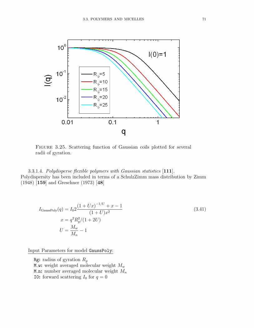
3.3. POLYMERS AND MICELLES 71
Figure 3.25. Scattering function of Gaussian coils plotted for severalradii of gyration.
3.3.1.4. Polydisperse flexible polymers with Gaussian statistics [111].Polydispersity has been included in terms of a SchulzZimm mass distribution by Zimm(1948) [159] and Greschner (1973) [48]
IGaussPoly(q) = I02(1 + Ux)−1/U + x− 1
(1 + U)x2(3.41)
x = q2R2g/(1 + 2U)
U =Mw
Mn
− 1
Input Parameters for model GaussPoly:
Rg: radius of gyration Rg
M w: weight averaged molecular weight Mw
M n: number averaged molecular weight Mn
I0: forward scattering I0 for q = 0
Gauss
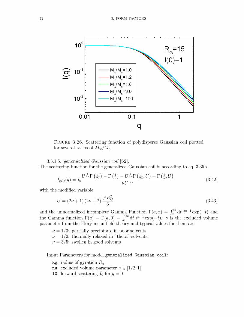
72 3. FORM FACTORS
Figure 3.26. Scattering function of polydisperse Gaussian coil plottedfor several ratios of Mw/Mn.
3.3.1.5. generalalized Gaussian coil [52].The scattering function for the generalized Gaussian coil is according to eq. 3.35b
IgGc(q) = I0
U12ν Γ(
12ν
)− Γ
(1ν
)− U 1
2ν Γ(
12ν, U)
+ Γ(
1ν, U)
νU1/ν(3.42)
with the modified variable
U = (2ν + 1) (2ν + 2)q2R2
G
6(3.43)
and the unnormalized incomplete Gamma Function Γ(a, x) =∫∞x
dt ta−1 exp(−t) and
the Gamma function Γ(a) = Γ(a, 0) =∫∞
0dt ta−1 exp(−t). ν is the excluded volume
parameter from the Flory mean field theory and typical values for them are
ν = 1/3: partially precipitate in poor solventsν = 1/2: thermally relaxed in ”theta”-solventsν = 3/5: swollen in good solvents
Input Parameters for model generalized Gaussian coil:
Rg: radius of gyration Rg
nu: excluded volume parameter ν ∈ [1/2; 1]I0: forward scattering I0 for q = 0
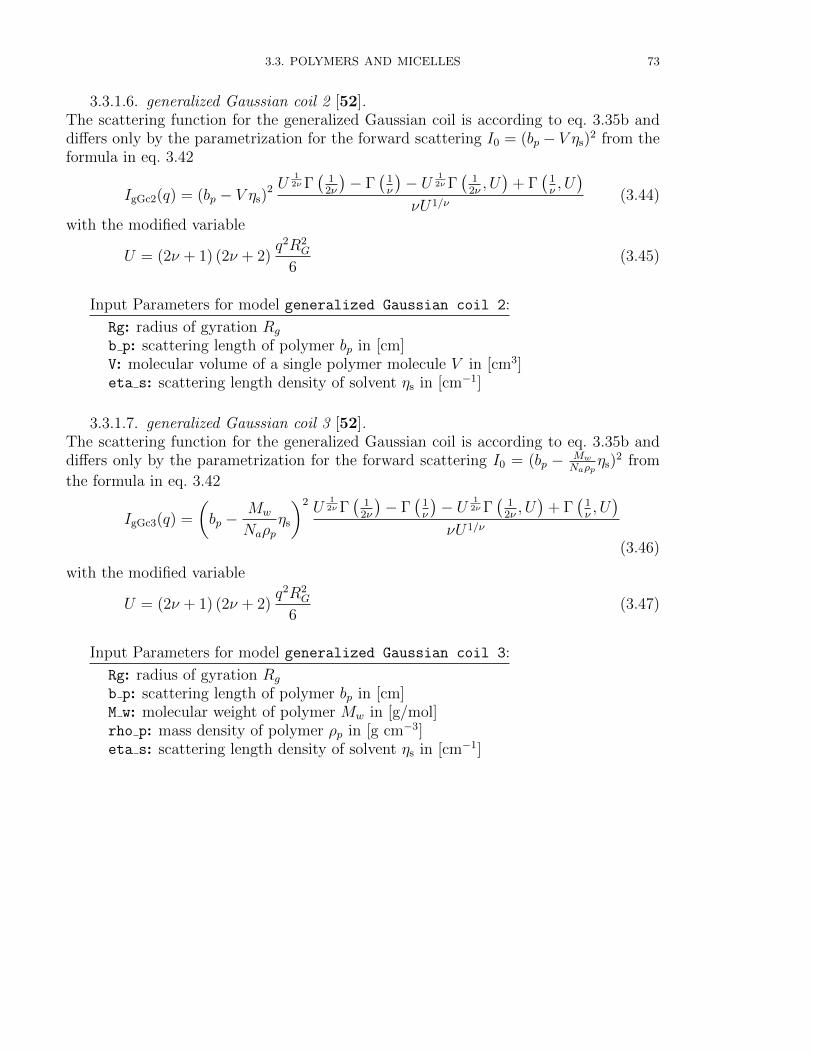
3.3. POLYMERS AND MICELLES 73
3.3.1.6. generalized Gaussian coil 2 [52].The scattering function for the generalized Gaussian coil is according to eq. 3.35b anddiffers only by the parametrization for the forward scattering I0 = (bp − V ηs)
2 from theformula in eq. 3.42
IgGc2(q) = (bp − V ηs)2 U
12ν Γ(
12ν
)− Γ
(1ν
)− U 1
2ν Γ(
12ν, U)
+ Γ(
1ν, U)
νU1/ν(3.44)
with the modified variable
U = (2ν + 1) (2ν + 2)q2R2
G
6(3.45)
Input Parameters for model generalized Gaussian coil 2:
Rg: radius of gyration Rg
b p: scattering length of polymer bp in [cm]V: molecular volume of a single polymer molecule V in [cm3]eta s: scattering length density of solvent ηs in [cm−1]
3.3.1.7. generalized Gaussian coil 3 [52].The scattering function for the generalized Gaussian coil is according to eq. 3.35b anddiffers only by the parametrization for the forward scattering I0 = (bp − Mw
Naρpηs)
2 from
the formula in eq. 3.42
IgGc3(q) =
(bp −
Mw
Naρpηs
)2 U12ν Γ(
12ν
)− Γ
(1ν
)− U 1
2ν Γ(
12ν, U)
+ Γ(
1ν, U)
νU1/ν
(3.46)
with the modified variable
U = (2ν + 1) (2ν + 2)q2R2
G
6(3.47)
Input Parameters for model generalized Gaussian coil 3:
Rg: radius of gyration Rg
b p: scattering length of polymer bp in [cm]M w: molecular weight of polymer Mw in [g/mol]rho p: mass density of polymer ρp in [g cm−3]eta s: scattering length density of solvent ηs in [cm−1]

74 3. FORM FACTORS
Figure 3.27. Scattering function of the generalized Gaussian coil plottedfor several excluded volume parameters.

3.3. POLYMERS AND MICELLES 75
3.3.2. Star polymer with Gaussian statistic according to Benoit [8].
Figure 3.28. Sketch of a branched or star polymers with f number of arms
Benoit [8] derived an expression for the scattering from branched or star polymerswith a number of arms f , which can be expressed in the following way:
IStar(Q,RG, f) = I02
fν2
(ν −
[1− e−ν
]+f − 1
2
[1− e−ν
]2)(3.48)
with u = R2GQ
2, ν =uf
3f − 2and lim
Q=0IStar(Q,RG, f) = I0. f denotes the number of arms
and RG the Guinier radius of a single arm.
Input Parameters for model Benoit:
RG: radius of gyration of the star polymer Rg
f: number of arms fI0: forward scattering I0 for q = 0
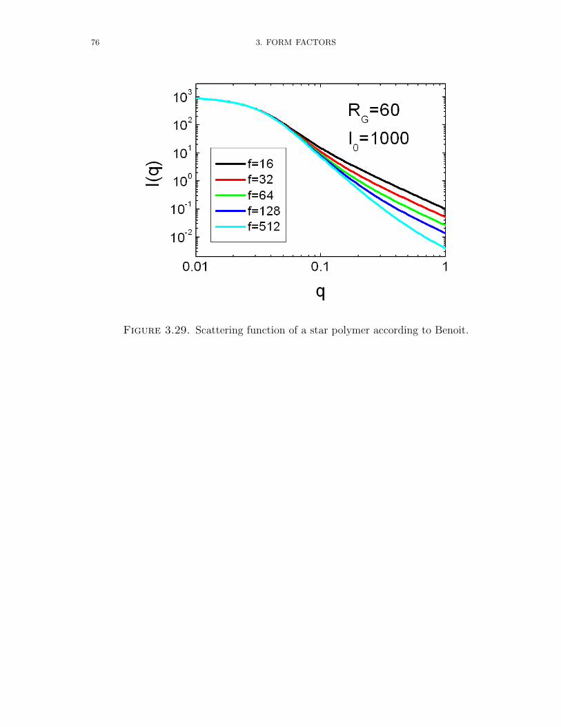
76 3. FORM FACTORS
Figure 3.29. Scattering function of a star polymer according to Benoit.
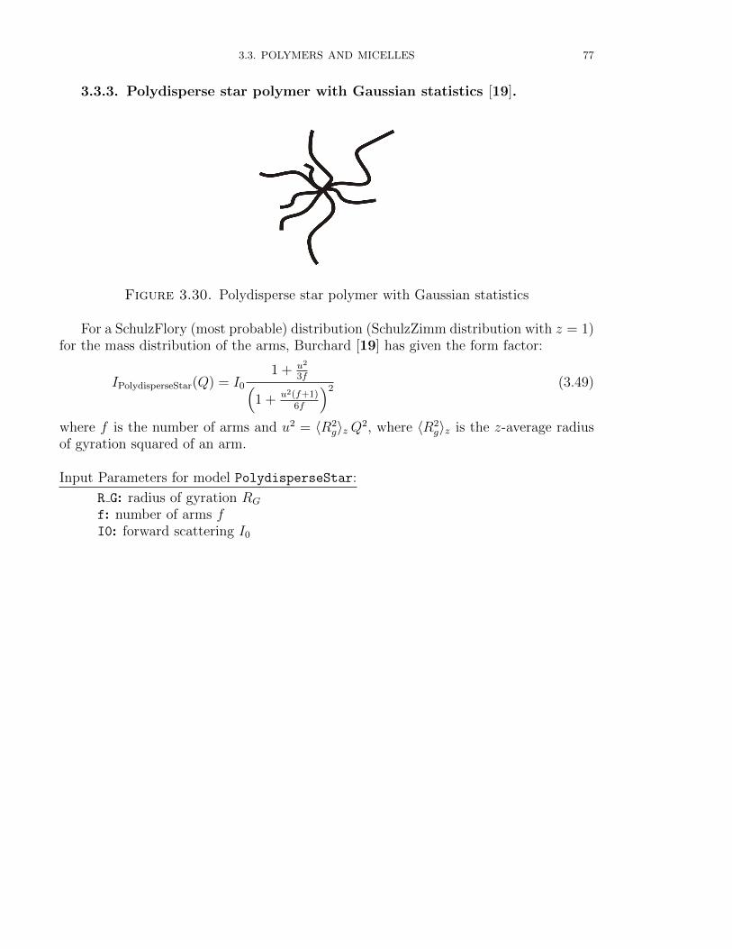
3.3. POLYMERS AND MICELLES 77
3.3.3. Polydisperse star polymer with Gaussian statistics [19].
Figure 3.30. Polydisperse star polymer with Gaussian statistics
For a SchulzFlory (most probable) distribution (SchulzZimm distribution with z = 1)for the mass distribution of the arms, Burchard [19] has given the form factor:
IPolydisperseStar(Q) = I0
1 + u2
3f(1 + u2(f+1)
6f
)2 (3.49)
where f is the number of arms and u2 = 〈R2g〉z Q2, where 〈R2
g〉z is the z-average radiusof gyration squared of an arm.
Input Parameters for model PolydisperseStar:
R G: radius of gyration RG
f: number of arms fI0: forward scattering I0
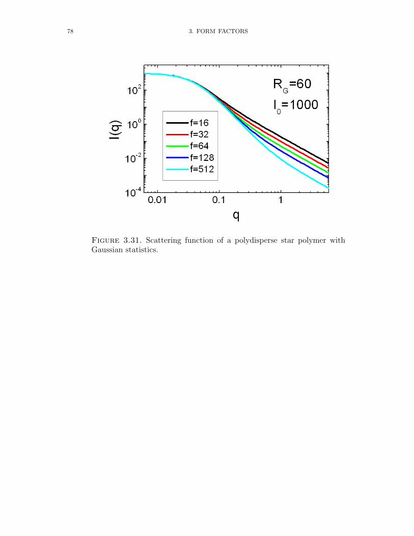
78 3. FORM FACTORS
Figure 3.31. Scattering function of a polydisperse star polymer withGaussian statistics.

3.3. POLYMERS AND MICELLES 79
3.3.4. Star polymer according to Dozier [35].
3.3.4.1. Dozier.Branched polymers having all branches emanating from the center of the macromolecule
Figure 3.32. Star polymer according to Dozier
are commonly called star polymers. For a star polymer Dozier [35] has developed ascattering function which reads:
IDozierStar(Q, I0, RG, α, ν, ξ) = I0 exp
(−Q
2R2G
3
)(3.50)
+4πα
QξΓ(µ)
sin(µ arctan(Qξ))
(1 +Q2ξ2)µ/2
with µ = 1/ν − 1
RG : radius of gyration
I0 : scale parameter
α : scale parameter for fractal term
ξ : exponential damping length in mass fractal
ν : Flory exponent, 3/5 in good solvent, 1/2 in theta solvent (i.e. µ = 2/3 to 1)
Input Parameters for model Dozier:
R G: radius of gyration RG
I 0: scale parameter I0
alpha: scale parameter for fractal term αxi: exponential damping length in mass fractal ξnu: excluded volume parameter or Flory exponent ν
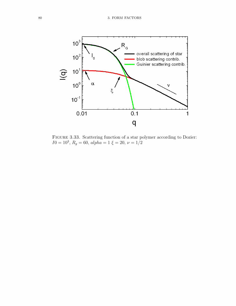
80 3. FORM FACTORS
Figure 3.33. Scattering function of a star polymer according to Dozier:I0 = 103, Rg = 60, alpha = 1 ξ = 20, ν = 1/2
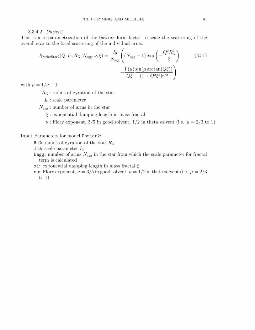
3.3. POLYMERS AND MICELLES 81
3.3.4.2. Dozier2.This is a re-parametrization of the Dozier form factor to scale the scattering of theoverall star to the local scattering of the individual arms.
IDozierStar2(Q, I0, RG, Nagg, ν, ξ) =I0
Nagg
((Nagg − 1) exp
(−Q
2R2G
3
)(3.51)
+Γ(µ)
Qξ
sin(µ arctan(Qξ))
(1 +Q2ξ2)µ/2
)with µ = 1/ν − 1
RG : radius of gyration of the star
I0 : scale parameter
Nagg : number of arms in the star
ξ : exponential damping length in mass fractal
ν : Flory exponent, 3/5 in good solvent, 1/2 in theta solvent (i.e. µ = 2/3 to 1)
Input Parameters for model Dozier2:
R G: radius of gyration of the star RG
I 0: scale parameter I0
Nagg: number of arms Nagg in the star from which the scale parameter for fractalterm is calculated
xi: exponential damping length in mass fractal ξnu: Flory exponent, ν = 3/5 in good solvent, ν = 1/2 in theta solvent (i.e. µ = 2/3
to 1)
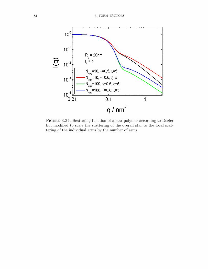
82 3. FORM FACTORS
Figure 3.34. Scattering function of a star polymer according to Dozierbut modified to scale the scattering of the overall star to the local scat-tering of the individual arms by the number of arms
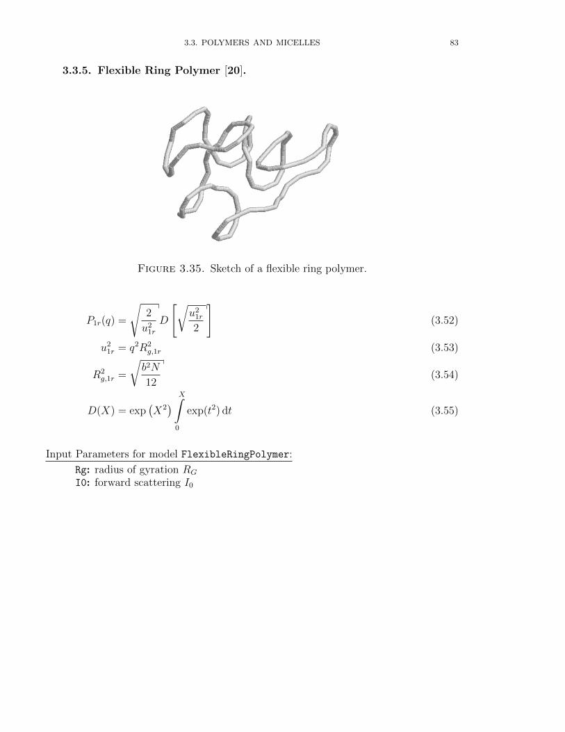
3.3. POLYMERS AND MICELLES 83
3.3.5. Flexible Ring Polymer [20].
Figure 3.35. Sketch of a flexible ring polymer.
P1r(q) =
√2
u21r
D
[√u2
1r
2
](3.52)
u21r = q2R2
g,1r (3.53)
R2g,1r =
√b2N
12(3.54)
D(X) = exp(X2) X∫
0
exp(t2) dt (3.55)
Input Parameters for model FlexibleRingPolymer:
Rg: radius of gyration RG
I0: forward scattering I0
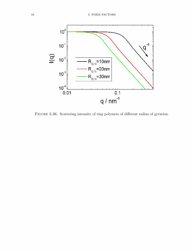
84 3. FORM FACTORS
Figure 3.36. Scattering intensity of ring polymers of different radius of gyration.
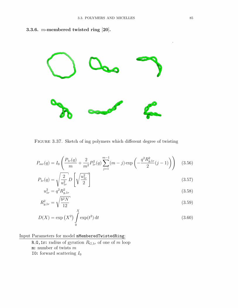
3.3. POLYMERS AND MICELLES 85
3.3.6. m-membered twisted ring [20].
Figure 3.37. Sketch of ing polymers which different degree of twisting
Pmr(q) = I0
(P1r(q)
m+
2
m2P 2
1r(q)m−1∑j=1
(m− j) exp
(−q2R2
g,1r
2(j − 1)
))(3.56)
P1r(q) =
√2
u21r
D
[√u2
1r
2
](3.57)
u21r = q2R2
g,1r (3.58)
R2g,1r =
√b2N
12(3.59)
D(X) = exp(X2) X∫
0
exp(t2) dt (3.60)
Input Parameters for model mMemberedTwistedRing:
R G,1r: radius of gyration RG,1r of one of m loopm: number of twists mI0: forward scattering I0
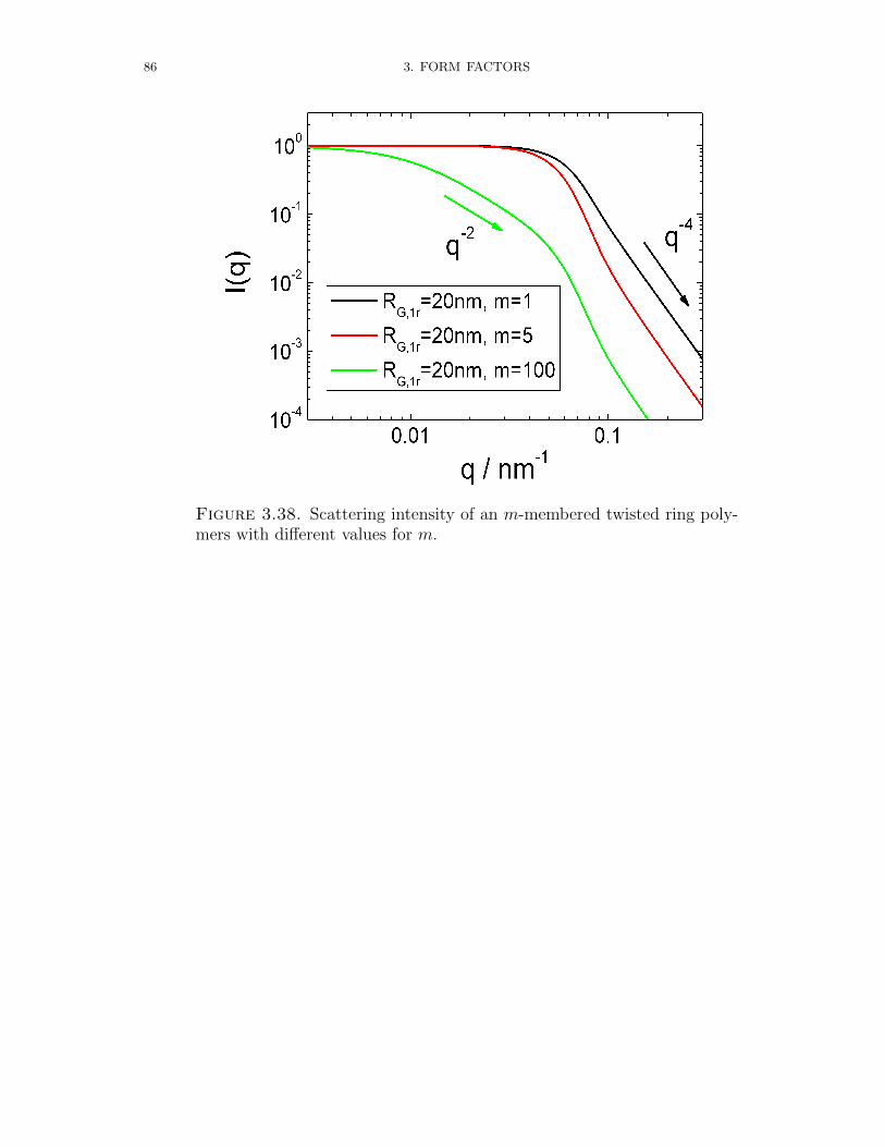
86 3. FORM FACTORS
Figure 3.38. Scattering intensity of an m-membered twisted ring poly-mers with different values for m.
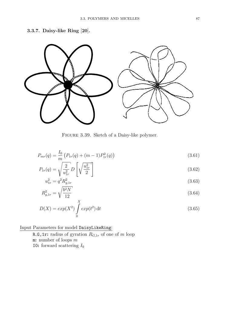
3.3. POLYMERS AND MICELLES 87
3.3.7. Daisy-like Ring [20].
Figure 3.39. Sketch of a Daisy-like polymer.
Pmr(q) =I0
m
(P1r(q) + (m− 1)P 2
1r(q))
(3.61)
P1r(q) =
√2
u21r
D
[√u2
1r
2
](3.62)
u21r = q2R2
g,1r (3.63)
R2g,1r =
√b2N
12(3.64)
D(X) = exp(X2)
X∫0
exp(t2) dt (3.65)
Input Parameters for model DaisyLikeRing:
R G,1r: radius of gyration RG,1r of one of m loopm: number of loops mI0: forward scattering I0
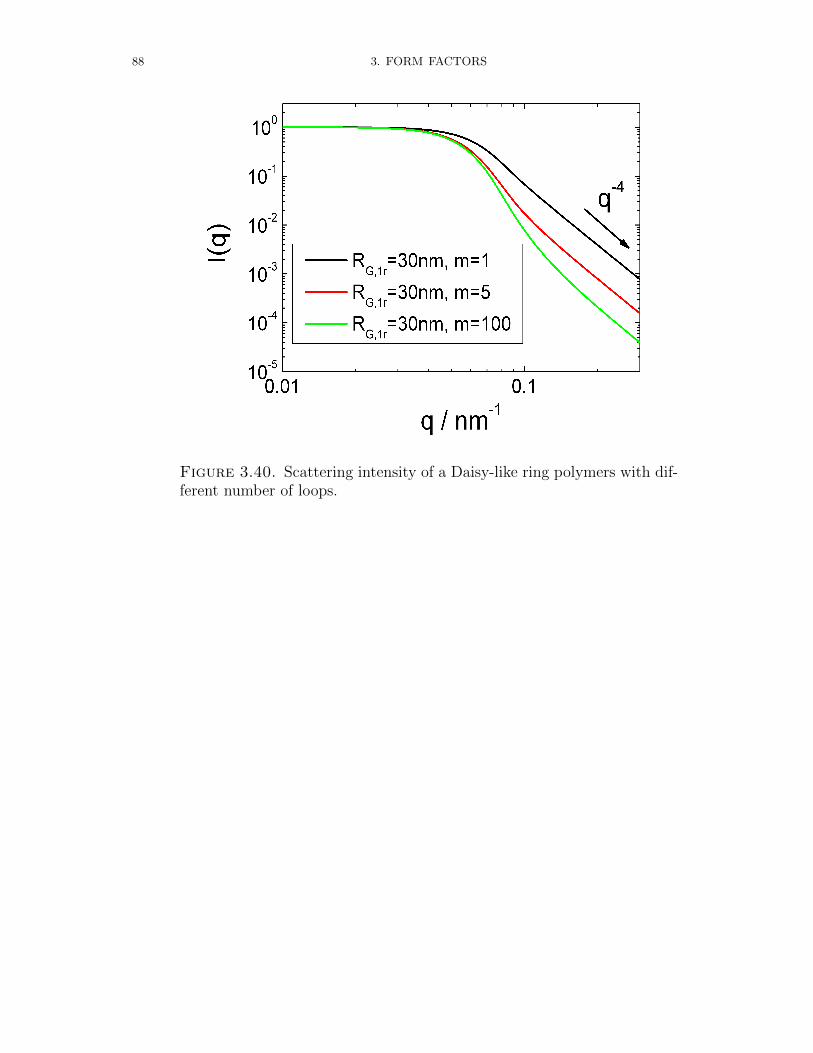
88 3. FORM FACTORS
Figure 3.40. Scattering intensity of a Daisy-like ring polymers with dif-ferent number of loops.

3.3. POLYMERS AND MICELLES 89
3.3.8. Unified Exponential Power Law according to Beaucage [6, 7].
Figure 3.41. A typical case in which two Rg’s are observed. Particlescomposed of sub-particles where a radius of gyration for the entire particle,Rg, and a radius of gyration for the sub-particles, Rs, are observed. Thesurface-fractal cut-off radius of gyration, Rsub, differs from the high-Qradius of gyration, Rs, in this case. Generally, Rs = Rsub
3.3.8.1. Beaucage.
IBeaucage(Q) ' G exp
(−Q2R2
g
3
)
+B exp
(−Q
2R2sub
3
)([erf(QkRg/
√6)]3
Q
)P
+Gs exp
(−Q
2R2s
3
)
+Bs
([erf(QksRs/
√6)]3
Q
)Ps
(3.66)
The first term in eq. 3.66 describes the large-scale structure of size Rg composed ofsmall subunits of size Rs, captured in the third term. The second term describes themass-fractal regime with two structural limits. The low-Q limit is at Rg and is describedby the error function. The high-Q limit is at Rsub and is described by the exponentialpre-factor [6] . The final two terms are for the sub-structural mer unit. Using eq. 3.66,scattering from a system with multiple-size-scale features is parameterized. Generally,the high-Q cutoff for the intermediate power law, Rsub, is identical to the sub-structuralradius of gyration, Rs. The assumption that Rsub = Rs should always be true for typical
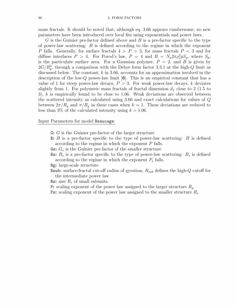
90 3. FORM FACTORS
mass fractals. It should be noted that, although eq. 3.66 appears cumbersome, no newparameters have been introduced over local fits using exponentials and power laws.
G is the Guinier pre-factor defined above and B is a pre-factor specific to the typeof power-law scattering: B is defined according to the regime in which the exponentP falls. Generally, for surface fractals 4 > P > 3, for mass fractals P < 3 and fordiffuse interfaces P > 4. For Porod’s law, P = 4 and B = Np2πρ
2cpSp, where Sp,
is the particulate surface area. For a Gaussian polymer, P = 2, and B is given by2G/R2
g, through a comparison with the Debye form factor 3.3.1 at the high-Q limit asdiscussed below. The constant, k in 3.66, accounts for an approximation involved in thedescription of the low-Q power-law limit [6]. This is an empirical constant that has avalue of 1 for steep power-law decays, P > 3. For weak power-law decays, k deviatesslightly from 1. For polymeric mass fractals of fractal dimension df close to 2 (1.5 to3), k is empirically found to be close to 1.06. Weak deviations are observed betweenthe scattered intensity as calculated using 3.66 and exact calculations for values of Qbetween 2π/Rg and π/Rg in these cases when k = 1. These deviations are reduced toless than 3% of the calculated intensity using k = 1.06.
Input Parameters for model Beaucage:
G: G is the Guinier pre-factor of the larger structureB: B is a pre-factor specific to the type of power-law scattering: B is defined
according to the regime in which the exponent P falls.Gs: Gs is the Guinier pre-factor of the smaller structureBs: Bs is a pre-factor specific to the type of power-law scattering: Bs is defined
according to the regime in which the exponent Ps falls.Rg: large-scale structureRsub: surface-fractal cut-off radius of gyration, Rsub defines the high-Q cutoff for
the intermediate power lawRs: size Rs of small subunitsP: scaling exponent of the power law assigned to the larger structure Rg
Ps: scaling exponent of the power law assigned to the smaller structure Rs
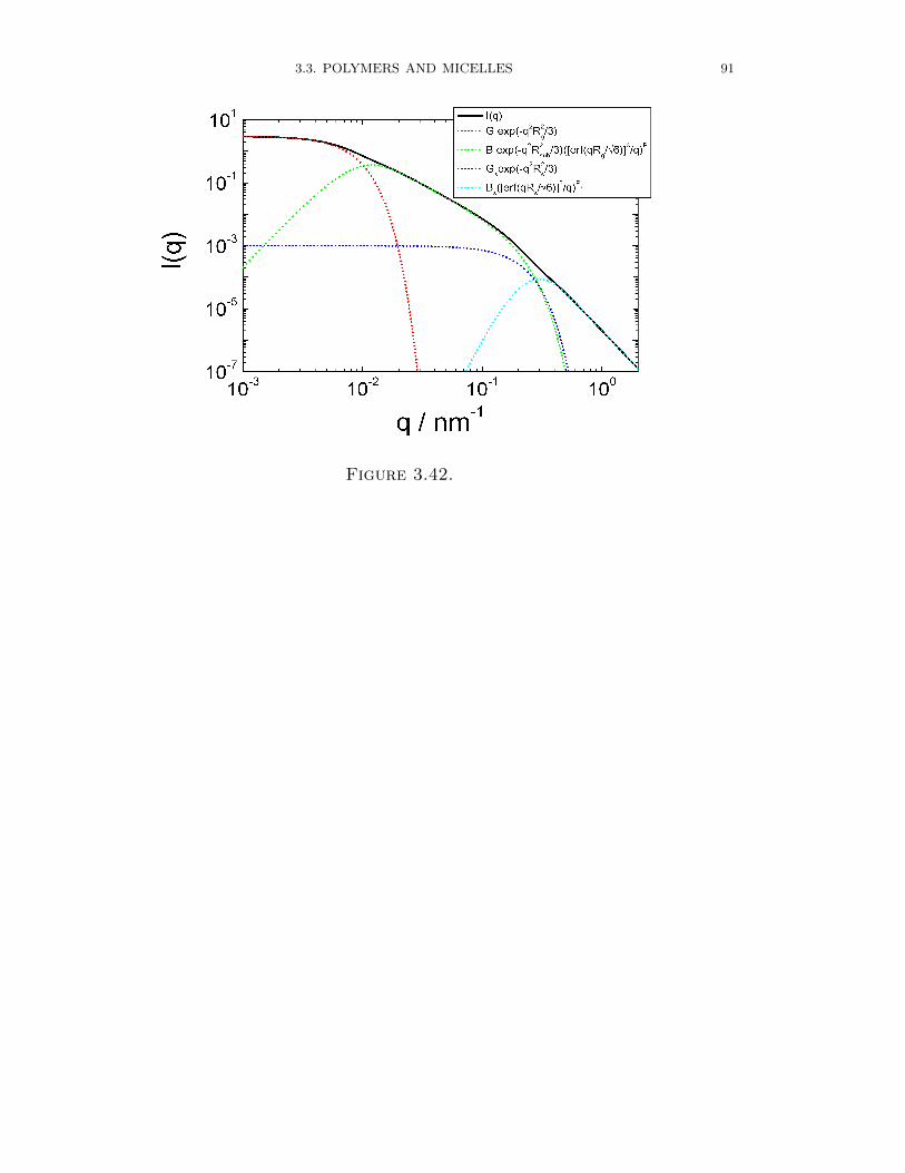
3.3. POLYMERS AND MICELLES 91
Figure 3.42.

92 3. FORM FACTORS
3.3.8.2. Beaucage2.
Equation 3.66 can be extended to describe an arbitrary number of interrelated struc-tural levels under the generally applicable assumption that Rsub = Rs,
IBeaucage(Q) 'n∑i=1
Gi exp
(−Q2R2
g,i
3
)
+Bi exp
(−Q2R2
g,i+1
3
)([erf(QkiRg,i/
√6)]3
Q
)Pi (3.67)
In 3.67, i = 1 refers to the largest-size structural level. Extensions, such as eq. 3.67, canonly be justified when data extend over many decades in Q. Eq. 3.67 introduces no newparameters over local Guinier and power-law fits.
Input Parameters for model Beaucage2:
G i: Gi is the Guinier pre-factorB i: Bi is a pre-factor specific to the type of power-law scattering: Bi is defined
according to the regime in which the exponent Pi falls.Rg i: large-scale structure Rg,i
Rg i+1: size Rg,i+1 of smaller subunitsk i: This is an empirical constant that has a value of 1 for steep power-law decays,P > 3. For weak power-law decays, k deviates slightly from 1
k i+1: This is an empirical constant that has a value of 1 for steep power-lawdecays, Ps > 3. For weak power-law decays, ks deviates slightly from 1
P i: scaling exponent of the power law assigned to the larger structure Rg,i
P i+1: scaling exponent of the power law assigned to the smaller structure Rg,i+1
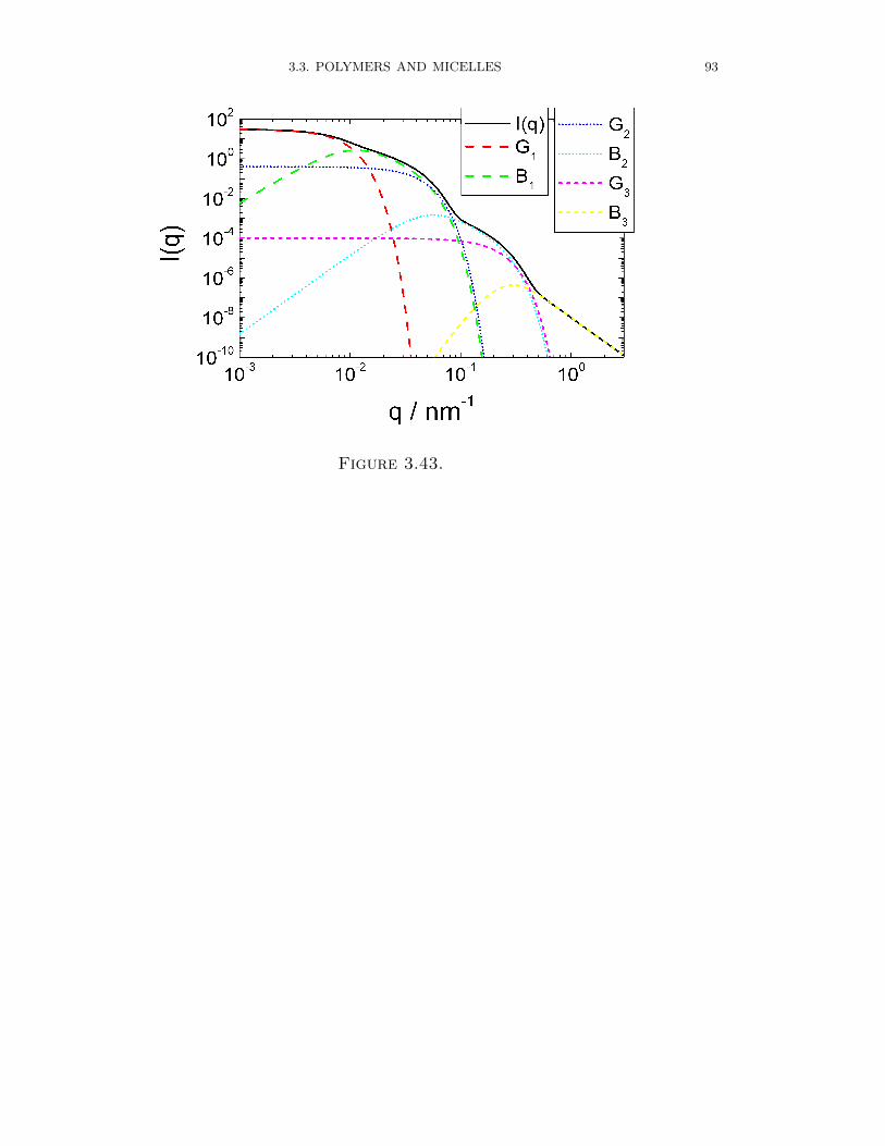
3.3. POLYMERS AND MICELLES 93
Figure 3.43.

94 3. FORM FACTORS
3.3.9. WormLikeChainEXV [110].
Figure 3.44. The chain of contour length, L, (the total length) can bedescribed a chain of some number of locally stiff segments of length lp.The persistence length,lp, is the length along the cylinder over which theflexible cylinder can be considered a rigid rod. The Kuhn length (b) usedin the model is also used to describe the stiffness of a chain, and is simplyb = 2lp.
This form factor calculates the form factor for a flexible cylinder with a circularcross section and a uniform scattering length density. The non-negligible diameter ofthe cylinder is included by accounting for excluded volume interactions within the walk ofa single cylinder. Inter-cylinder interactions are NOT included. The function calculatedhas been given by Pedersen et al. [110]. The model ”Method 3 With Excluded Volume”is used, which is a parametrization of simulations of a discrete representation of theworm-like chain model of Kratky and Porod applied in the pseudo-continuous limit.
Input Parameters for model WormLikeChainEXV:
R: radius R of cylindrical core with uniform scattering length densityl: Kuhn length3 l of semi-flexible worm-like structureL: contour length L of semi-flexible worm-like structure
3The Kuhn length l is related to the length a of locally stiff segment simply via l = 2a
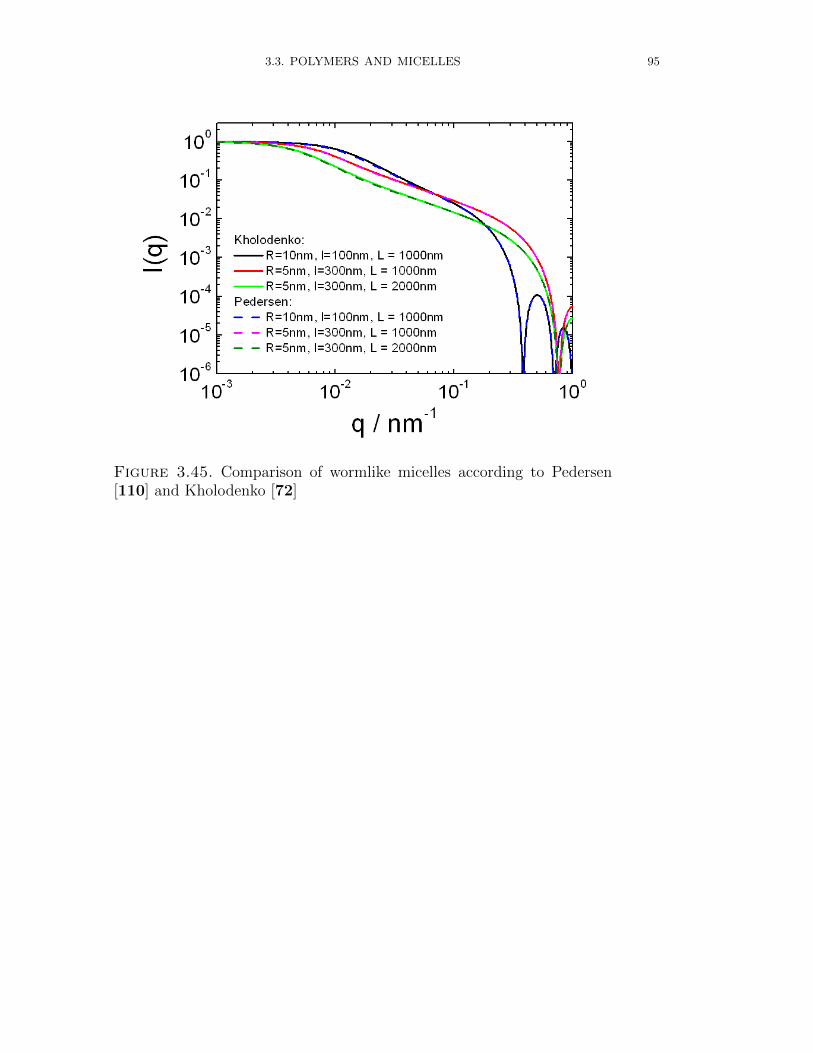
3.3. POLYMERS AND MICELLES 95
Figure 3.45. Comparison of wormlike micelles according to Pedersen[110] and Kholodenko [72]

96 3. FORM FACTORS
3.3.10. KholodenkoWorm.
Figure 3.46.
Kholodenko [72] presented a new approach using the analogy between Diracsfermions and semi-flexible polymers. The form factor P0(Q) resulting from Kholodenkosapproach is designed to reproduce correctly the rigid-rod limit and the random-coil limit.Defining x = 3L/l (L: contour length, l: Kuhn length), it is given by
P0(Q,L, l) =2
x
[I(1) −
1
xI(2)
](3.68)
where
I(n)(x) =
x∫0
f(z) zn−1 dz (3.69)
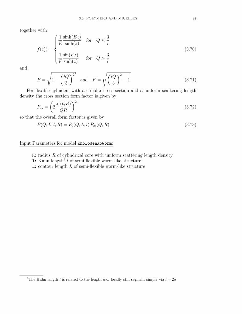
3.3. POLYMERS AND MICELLES 97
together with
f(z)) =
1
E
sinh(Ez)
sinh(z)for Q ≤ 3
l
1
F
sin(Fz)
sinh(z)for Q >
3
l
(3.70)
and
E =
√1−
(lQ
3
)2
and F =
√(lQ
3
)2
− 1 (3.71)
For flexible cylinders with a circular cross section and a uniform scattering lengthdensity the cross section form factor is given by
Pcs =
(2J1(QR)
QR
)2
(3.72)
so that the overall form factor is given by
P (Q,L, l, R) = P0(Q,L, l)Pcs(Q,R) (3.73)
Input Parameters for model KholodenkoWorm:
R: radius R of cylindrical core with uniform scattering length densityl: Kuhn length4 l of semi-flexible worm-like structureL: contour length L of semi-flexible worm-like structure
4The Kuhn length l is related to the length a of locally stiff segment simply via l = 2a

98 3. FORM FACTORS
Figure 3.47. Comparison of wormlike micelles according to Pedersen[110] and Kholodenko [72].

3.3. POLYMERS AND MICELLES 99
3.3.11. Diblock copolymer micelles.
(a) spherical micelle (b) ellipsoidal micelle (c) cylindrical micelle
Figure 3.48. Block copolymer forming micelles of different shapes
For block copolymers, which form micelles, several form factor have been imple-mented [112, 113, 134] for spherical, ellipsoidal, and cylindrical shapes. It has beenassumed that one unit is forming the core of the micelles and the other the corona. Thecore is assumed to have a homogeneous scattering length density, but may contain someamount of solvent. For the polymer chains in the corona either a model where Gaussianchains are attached to the core or a corona model of semi-flexible interacting self-avoidingchains (only for spherical core) or a continuous model, where a radial profile of the formΦ(r) ∝ r−α has been assumed. The form factors have been parameterized such, thatthe excess scattering of the corona and the core are consistent with the composition anddensity of the two separate block units of the copolymer.
3.3.11.1. Micelles with a homogeneous core and Gaussian chains on the surface.
It is assumed that the diblock copolymer consist of a block unit for which the sol-vent is poor and a block unit with is good. The insoluble blocks form a relativelycompact core whereas the soluble blocks form a diffuse corona surrounding the core.The form factor of a micelle contains four different terms: the self-correlation term ofthe core N2
aggβ2core Pcore(q), the self-correlation term of the chains Naggβ
2brush Pbrush(q), the
cross-term between the core and chains 2N2aggβcoreβbrush Sbrush-core(q), and the cross term
between different chains Nagg(Nagg − 1)β2brush Sbrush-brush(q). It can be written (Pedersen
& Gerstenberg, 1996)
Imic = N2aggβ
2core Pcore(q) +Naggβ
2brush Pbrush(q) (3.74)
+ 2N2aggβcoreβbrush Sbrush-core(q) +Nagg(Nagg − 1)β2
brush Sbrush-brush(q)

100 3. FORM FACTORS
Nagg is the aggregation number of diblock polymers forming the micelle and βbrush =Vbrush(ηbrush− ηsolv) and βcore = Vcore(ηcore− ηsolv) the excess scattering length of a blockin the corona and in the core, respectively. Vbrush and Vcore are the total volume of ablock in the corona and in the core. ηbrush and ηcore are the corresponding scatteringlength densities and ηsolv is the scattering length density of the surrounding solvent.The functions Pcore(q), Pbrush(q), Sbrush-core(q), and Sbrush-brush(q) are all 1 for q = 0. Thedefinitions of these four functions depend on the shape of the core and are given below.
3.3.11.2. Spherical core:
Pcore(q, Rcore) = Φ2(qRcore) (3.75)
Φ(qR) = 3sin(qR)− qR cos(qR)
(qR)3(3.76)
Pbrush(q, Rg) = 2exp(−x)− 1 + x
x2with x = R2
gq2 (3.77)
Sbrush-core(q, Rcore, Rg, d) = Φ(qRcore)ψ(qRg)sin(q[Rcore + dRg])
q[Rcore + dRg](3.78)
ψ(qRg) =1− exp(−x)
x(form factor amplitude of the chain)
Sbrush-brush(q, Rcore, d, Rg) = ψ2(qRg)
[sin(q[Rcore + dRg])
q[Rcore + dRg]
]2
(3.79)
For micelles with a spherical core a few different parameterizations have been imple-mented SPHERE+Chains(RW), SPHERE+Chains(RW) Rc and SPHERE+Chains(RW) Nagg.The parameters they all have in common are:
Vbrush: molecular volume the diblock copolymer part forming the coronaηcore: scattering length density of the diblock copolymer part forming the coreηbrush: scattering length density of the diblock copolymer part forming the coronaηsolv: scattering length density of the solventxsolv,core: volume fraction of solvent in the micellar coreRg: radius of gyration of the block unit in the coronad: non-penetration of the chains into the core is mimicked by d ∼ 1 for Rcore Rg
For the model SPHERE+Chains(RW) the other parameters are
Rcore: radius of the micellar corenagg: grafting density (number of copolymer molecules Nagg per surface are S,nagg = Nagg/S)
In contrast to the form factor SPHERE+Chains(RW) Rc and SPHERE+Chains(RW) Nagg
this one does not necessary consist of copolymers. The excess scattering lengths and

3.3. POLYMERS AND MICELLES 101
aggregation number needed in eq. 3.74 are than given by
Nagg = naggS (3.80)
where the surface of the core is given by S = 4πR2core. Together with the core volume
V = 43πR3
core one gets for the excess scattering lengths
βcore =V (1− xsolv,core)
Nagg
(ηcore − ηsolv) (3.81)
βbrush = Vbrush(ηbrush − ηsolv) (3.82)
Input Parameters for model SPHERE+Chains(RW):
R core: core radiusn agg: specific aggregation number (number of chains per surface area)V brush: molecular volume of a block unit in the micellar coronaeta core: scattering length density of spherical coreeta brush: scattering length density of the block unit in the coronaeta solv: scattering length density of solventxsolv core: amount of solvent in coreRg: gyration radius of polymer chains in the coronad: This value should be around 1. Non-penetration of the chains into the core is
mimicked by d ∼ 1 for Rcore Rg
For the model SPHERE+Chains(RW) Rc the other parameters are
Rcore: core radiusVcore: molecular volume of single block unit in the micellar core
The excess scattering lengths and aggregation number in eq. 3.74 are given by
βcore = Vcore(ηcore − ηsolv) (3.83)
βbrush = Vbrush(ηbrush − ηsolv) (3.84)
Nagg = (1− xsolv,core)4
3πR3
core/Vcore (3.85)
Input Parameters for model SPHERE+Chains(RW) Rc:
R core: core radiusV core: molecular volume of single block unit in the micellar coreV brush: molecular volume of single block unit in the micellar coronaeta core: scattering length density of spherical coreeta brush: scattering length density of the block unit in the coronaeta solv: scattering length density of solventxsolv core: amount of solvent in coreRg: gyration radius of polymer chains in the corona
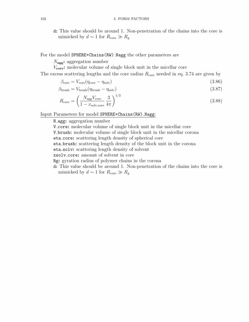
102 3. FORM FACTORS
d: This value should be around 1. Non-penetration of the chains into the core ismimicked by d ∼ 1 for Rcore Rg
For the model SPHERE+Chains(RW) Nagg the other parameters are
Nagg: aggregation numberVcore: molecular volume of single block unit in the micellar core
The excess scattering lengths and the core radius Rcore needed in eq. 3.74 are given by
βcore = Vcore(ηcore − ηsolv) (3.86)
βbrush = Vbrush(ηbrush − ηsolv) (3.87)
Rcore =
(NaggVcore
1− xsolv,core
3
4π
)1/3
(3.88)
Input Parameters for model SPHERE+Chains(RW) Nagg:
N agg: aggregation numberV core: molecular volume of single block unit in the micellar coreV brush: molecular volume of single block unit in the micellar coronaeta core: scattering length density of spherical coreeta brush: scattering length density of the block unit in the coronaeta solv: scattering length density of solventxsolv core: amount of solvent in coreRg: gyration radius of polymer chains in the coronad: This value should be around 1. Non-penetration of the chains into the core is
mimicked by d ∼ 1 for Rcore Rg
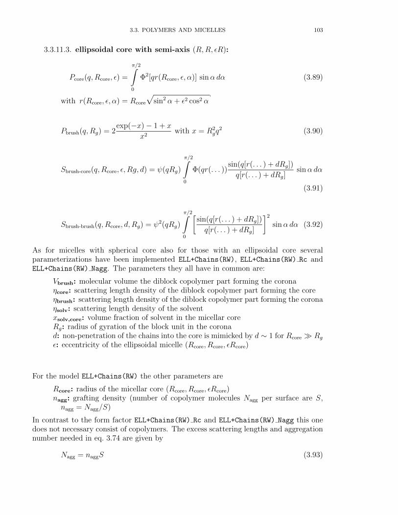
3.3. POLYMERS AND MICELLES 103
3.3.11.3. ellipsoidal core with semi-axis (R,R, εR):
Pcore(q, Rcore, ε) =
π/2∫0
Φ2[qr(Rcore, ε, α)] sinα dα (3.89)
with r(Rcore, ε, α) = Rcore
√sin2 α + ε2 cos2 α
Pbrush(q, Rg) = 2exp(−x)− 1 + x
x2with x = R2
gq2 (3.90)
Sbrush-core(q, Rcore, ε, Rg, d) = ψ(qRg)
π/2∫0
Φ(qr(. . . ))sin(q[r(. . . ) + dRg])
q[r(. . . ) + dRg]sinα dα
(3.91)
Sbrush-brush(q, Rcore, d, Rg) = ψ2(qRg)
π/2∫0
[sin(q[r(. . . ) + dRg])
q[r(. . . ) + dRg]
]2
sinα dα (3.92)
As for micelles with spherical core also for those with an ellipsoidal core severalparameterizations have been implemented ELL+Chains(RW), ELL+Chains(RW) Rc andELL+Chains(RW) Nagg. The parameters they all have in common are:
Vbrush: molecular volume the diblock copolymer part forming the coronaηcore: scattering length density of the diblock copolymer part forming the coreηbrush: scattering length density of the diblock copolymer part forming the coronaηsolv: scattering length density of the solventxsolv,core: volume fraction of solvent in the micellar coreRg: radius of gyration of the block unit in the coronad: non-penetration of the chains into the core is mimicked by d ∼ 1 for Rcore Rg
ε: eccentricity of the ellipsoidal micelle (Rcore, Rcore, εRcore)
For the model ELL+Chains(RW) the other parameters are
Rcore: radius of the micellar core (Rcore, Rcore, εRcore)nagg: grafting density (number of copolymer molecules Nagg per surface are S,nagg = Nagg/S)
In contrast to the form factor ELL+Chains(RW) Rc and ELL+Chains(RW) Nagg this onedoes not necessary consist of copolymers. The excess scattering lengths and aggregationnumber needed in eq. 3.74 are given by
Nagg = naggS (3.93)
104 3. FORM FACTORS
where the surface of the core is given by
S =
2πR2core
(1 + arctanh(sin(æ))
sin(æ)
)for ε < 1
2πR2core
(1 + æ
tan(æ)
)for ε ≥ 1
(3.94)
æ =
arccos(ε) for ε < 1
arccos(1/ε) for ε ≥ 1
Together with the core volume V = 43πεR3
core one gets for the excess scattering lengths
βcore =V (1− xsolv,core)
Nagg
(ηcore − ηsolv) (3.95)
βbrush = Vbrush(ηbrush − ηsolv) (3.96)
Input Parameters for model ELL+Chains(RW):
R core: core radiusn agg: specific aggregation number (number of chains per surface area)V brush: molecular volume of a block unit in the micellar coronaeta core: scattering length density of spherical coreeta brush: scattering length density of the block unit in the coronaeta solv: scattering length density of solventxsolv core: amount of solvent in coreRg: gyration radius of polymer chains in the coronad: This value should be around 1. Non-penetration of the chains into the core is
mimicked by d ∼ 1 for Rcore Rg
epsilon: eccentricity of the ellipsoidal micelle (Rcore, Rcore, εRcore)
For the model ELL+Chains(RW) Rc the other parameters are
Rcore: core radiusVcore: molecular volume of single block unit in the micellar core
The excess scattering lengths and aggregation number in eq. 3.74 are given by
βcore = Vcore(ηcore − ηsolv) (3.97)
βbrush = Vbrush(ηbrush − ηsolv) (3.98)
Nagg = (1− xsolv,core)4
3πεR3
core/Vcore (3.99)
Input Parameters for model ELL+Chains(RW) Rc:
R core: core radiusV core: molecular volume of single block unit in the micellar coreV brush: molecular volume of single block unit in the micellar coronaeta core: scattering length density of spherical coreeta brush: scattering length density of the block unit in the corona
3.3. POLYMERS AND MICELLES 105
eta solv: scattering length density of solventxsolv core: amount of solvent in coreRg: gyration radius of polymer chains in the coronad: This value should be around 1. Non-penetration of the chains into the core is
mimicked by d ∼ 1 for Rcore Rg
epsilon: eccentricity of the ellipsoidal micelle (Rcore, Rcore, εRcore)
For the model ELL+Chains(RW) Nagg the other parameters are
Nagg: aggregation numberVcore: molecular volume of single block unit in the micellar core
The excess scattering lengths and the core radius Rcore needed in eq. 3.74 are given by
βcore = Vcore(ηcore − ηsolv) (3.100)
βbrush = Vbrush(ηbrush − ηsolv) (3.101)
Rcore =
(NaggVcore
1− xsolv,core
3
4πε
)1/3
(3.102)
Input Parameters for model ELL+Chains(RW) Nagg:
N agg: aggregation numberV core: molecular volume of single block unit in the micellar coreV brush: molecular volume of single block unit in the micellar coronaeta core: scattering length density of spherical coreeta brush: scattering length density of the block unit in the coronaeta solv: scattering length density of solventxsolv core: amount of solvent in coreRg: gyration radius of polymer chains in the coronad: This value should be around 1. Non-penetration of the chains into the core is
mimicked by d ∼ 1 for Rcore Rg
epsilon: eccentricity of the ellipsoidal micelle (Rcore, Rcore, εRcore)
106 3. FORM FACTORS
3.3.11.4. cylindrical core with radius Rcore and height H:
Pcore(q, Rcore, H) =
π/2∫0
Ψ2(q, Rcore, H, α) sinα dα (3.103)
with Ψ(q, Rcore, H, α) =2J1(qRcore sinα)
qRcore sinα
sin(qH/2 cosα)
qH/2 cosα(3.104)
and J1(x) is the first order Bessel function of the first kind.
Pbrush(q, Rg) = 2exp(−x)− 1 + x
x2with x = R2
gq2 (3.105)
Sbrush-core(q,Rcore, H,Rg, d) = ψ(qRg) × (3.106)
π/2∫0
Ψ(q, Rcore, H, α)Ξ(q, R + dRg, H + 2dRg, α) sinα dα
where Ξ(q, Rcore, H, α) is the form factor amplitude of the shell:
Ξ(q, RcoreH,α) =
[R
Rcore +H
2J1(qRcore sinα)
qRcore sinαcos(qH/2 cosα) (3.107)
+H
Rcore +HJ0(qRcore sinα)
sin(qH/2 cosα)
qH/2 cosα
]where J0(x) is the zeroth order Bessel function of the first kind.
Sbrush-brush(q,Rcore, H, d, Rg) = ψ2(qRg) × (3.108)
π/2∫0
Ξ2(q, Rcore + dRg, H + 2dRg, α) sinα dα
As for micelles with spherical core also for those with a cylindrical core severalparameterizations have been implemented CYL+Chains(RW), CYL+Chains(RW) Rc andCYL+Chains(RW) Nagg. The parameters they all have in common are:
Vbrush: molecular volume the diblock copolymer part forming the coronaηcore: scattering length density of the diblock copolymer part forming the coreηbrush: scattering length density of the diblock copolymer part forming the coronaηsolv: scattering length density of the solventxsolv,core: volume fraction of solvent in the micellar coreRg: radius of gyration of the block unit in the coronad: non-penetration of the chains into the core is mimicked by d ∼ 1 for Rcore Rg
H: height of the cylindrical core of the micelle
For the model CYL+Chains(RW) the other parameters are
Rcore: radius of the micellar core (Rcore, Rcore, εRcore)

3.3. POLYMERS AND MICELLES 107
nagg: grafting density (number of copolymer molecules Nagg per surface are S,nagg = Nagg/S)
In contrast to the form factor CYL+Chains(RW) Rc and CYL+Chains(RW) Nagg this onedoes not necessary consist of copolymers. The excess scattering lengths and aggregationnumber needed in eq. 3.74 are than given by
Nagg = naggS (3.109)
where the surface of the core is given by
S = 2πRcoreH (3.110)
Together with the core volume V = πR2coreH one can calculate the excess scattering
lengths by
βcore =V (1− xsolv,core)
Nagg
(ηcore − ηsolv) (3.111)
βbrush = Vbrush(ηbrush − ηsolv) (3.112)
Input Parameters for model CYL+Chains(RW):
R core: core radiusn agg: specific aggregation number (number of chains per surface area)V brush: molecular volume of a block unit in the micellar coronaeta core: scattering length density of spherical coreeta brush: scattering length density of the block unit in the coronaeta solv: scattering length density of solventxsolv core: amount of solvent in coreRg: gyration radius of polymer chains in the coronad: This value should be around 1. Non-penetration of the chains into the core is
mimicked by d ∼ 1 for Rcore Rg
H: height of the cylindrical core of the micelle
For the model CYL+Chains(RW) Rc the other parameters are
Rcore: core radiusVcore: molecular volume of single block unit in the micellar core
The excess scattering lengths and aggregation number in eq. 3.74 are than given by
βcore = Vcore(ηcore − ηsolv) (3.113)
βbrush = Vbrush(ηbrush − ηsolv) (3.114)
Nagg = (1− xsolv,core)πR2coreH/Vcore (3.115)
Input Parameters for model CYL+Chains(RW) Rc:
R core: core radiusV core: molecular volume of single block unit in the micellar coreV brush: molecular volume of single block unit in the micellar coronaeta core: scattering length density of spherical core

108 3. FORM FACTORS
eta brush: scattering length density of the block unit in the coronaeta solv: scattering length density of solventxsolv core: amount of solvent in coreRg: gyration radius of polymer chains in the coronad: This value should be around 1. Non-penetration of the chains into the core is
mimicked by d ∼ 1 for Rcore Rg
H: height of the cylindrical core of the micelle
For the model CYL+Chains(RW) Nagg the other parameters are
Nagg: aggregation numberVcore: molecular volume of single block unit in the micellar core
The excess scattering lengths and the core radius Rcore are given by
βcore = Vcore(ηcore − ηsolv) (3.116)
βbrush = Vbrush(ηbrush − ηsolv) (3.117)
Rcore =
√NaggVcore
1− xsolv,core
1
πH(3.118)
Input Parameters for model CYL+Chains(RW) Nagg:
N agg: aggregation numberV core: molecular volume of single block unit in the micellar coreV brush: molecular volume of single block unit in the micellar coronaeta core: scattering length density of spherical coreeta brush: scattering length density of the block unit in the coronaeta solv: scattering length density of solventxsolv core: amount of solvent in coreRg: gyration radius of polymer chains in the coronad: This value should be around 1. Non-penetration of the chains into the core is
mimicked by d ∼ 1 for Rcore Rg
H: height of the cylindrical core of the micelle

3.3. POLYMERS AND MICELLES 109
3.3.11.5. wormlike micelles with cylindrical cross-section with radius Rcore,Kuhn-length l and contour length L:The form factors for a worm-like micelles are approximated by the form factor of theKholodenko-worm according to section 3.3.10 where the scattering length density profileacross the worm segments are described by those of a rod-like micelle 3.3.11.6. Thecorresponding function in eq. 3.74 are given by
Pcore(q, Rcore, l, L) = Pworm(q, l, L)Pcs(q, Rcore, d, Rg) (3.119)
the contributiion of the worm-like conformation of the micelle Pworm(q, l, L) is describedby the formula of Kholodenko for worm-like structures given in eq. 3.68. The contribu-tion of the cross-section Pcs is the same as for rod-like micelles and given by
Pcs(q, Rcore, d, Rg) =
[2J1(qRcore)
qRcore
]2
(3.120)
Si(x) =
x∫0
t−1 sin t dt (3.121)
Pbrush(q, Rg) = 2exp(−x)− 1 + x
x2with x = R2
gq2 (3.122)
Sbrush-core(q,Rcore, l, L,Rg, d) = ψ(qRg) × (3.123)
2J1(qRcore)
qRcore
J0[q(rcore + dRg)]Pworm(q, l, L)
Sbrush-brush(q, Rcore, l, L, d, Rg) = ψ2(qRg)J20 [q(rcore + dRg)]Pworm(q, l, L) (3.124)
As for micelles with spherical core also for those worm-like micelles several pa-rameterizations have been implemented WORM+Chains(RW), WORM+Chains(RW) Rc andWORM+Chains(RW) nagg. The parameters they all have in common are:
Vbrush: molecular volume the diblock copolymer part forming the coronaηcore: scattering length density of the diblock copolymer part forming the coreηbrush: scattering length density of the diblock copolymer part forming the coronaηsolv: scattering length density of the solventxsolv,core: volume fraction of solvent in the micellar coreRg: radius of gyration of the block unit in the coronal: contour length of the worm-like of the micelleL: contour length of the worm-like of the micelle
For the model WORM+Chains(RW) the other parameters are
Rcore: radius of the micellar corenagg: grafting density (number of copolymer molecules Nagg per surface are S,nagg = Nagg/S)
110 3. FORM FACTORS
In contrast to the form factor WORM+Chains(RW) Rc and WORM+Chains(RW) nagg this onedoes not necessary consist of copolymers. The excess scattering lengths and aggregationnumber needed in eq. 3.74 are than given by
Nagg = naggS (3.125)
where the surface of the core is given by
S = 2πRcoreL (3.126)
Together with the core volume V = πR2coreL one can calculate the excess scattering
lengths by
βcore =V (1− xsolv,core)
Nagg
(ηcore − ηsolv) (3.127)
βbrush = Vbrush(ηbrush − ηsolv) (3.128)
Input Parameters for model WORM+Chains(RW):
R core: core radiusn agg: specific aggregation number (number of chains per surface area)V brush: molecular volume of a block unit in the micellar coronaeta core: scattering length density of spherical coreeta brush: scattering length density of the block unit in the coronaeta solv: scattering length density of solventxsolv core: amount of solvent in coreRg: gyration radius of polymer chains in the coronal: contour length of the worm-like of the micelleL: contour length of the worm-like of the micelle
For the model WORM+Chains(RW) Rc the other parameters are
Rcore: core radiusVcore: molecular volume of single block unit in the micellar core
The excess scattering lengths and aggregation number in eq. 3.74 are than given by
βcore = Vcore(ηcore − ηsolv) (3.129)
βbrush = Vbrush(ηbrush − ηsolv) (3.130)
Nagg = (1− xsolv,core)πR2coreL/Vcore (3.131)
Input Parameters for model CYL+Chains(RW) Rc:
R core: core radiusV core: molecular volume of single block unit in the micellar coreV brush: molecular volume of single block unit in the micellar coronaeta core: scattering length density of spherical coreeta brush: scattering length density of the block unit in the coronaeta solv: scattering length density of solventxsolv core: amount of solvent in core
3.3. POLYMERS AND MICELLES 111
Rg: gyration radius of polymer chains in the coronal: contour length of the worm-like of the micelleL: contour length of the worm-like of the micelle
For the model WORM+Chains(RW) Nagg the other parameters are
Nagg: aggregation numberVcore: molecular volume of single block unit in the micellar core
The excess scattering lengths and the core radius Rcore are given by
βcore = Vcore(ηcore − ηsolv) (3.132)
βbrush = Vbrush(ηbrush − ηsolv) (3.133)
Rcore =
√NaggVcore
1− xsolv,core
1
πL(3.134)
Input Parameters for model CYL+Chains(RW) Nagg:
N agg: aggregation numberV core: molecular volume of single block unit in the micellar coreV brush: molecular volume of single block unit in the micellar coronaeta core: scattering length density of spherical coreeta brush: scattering length density of the block unit in the coronaeta solv: scattering length density of solventxsolv core: amount of solvent in coreRg: gyration radius of polymer chains in the coronal: contour length of the worm-like of the micelleL: contour length of the worm-like of the micelle

112 3. FORM FACTORS
3.3.11.6. micelles with rod-like core:The form factors for micelles with a rod-like core are an approximations of the formfactors of micelles with a cylindrical core where H Rcore + dRg. The correspondingfunction in eq. 3.74 are given by
Pcore(q, Rcore, H) = PH(q,H)Pcs(q, Rcore, d, Rg) (3.135)
with
PH(q,H) = 2Si(qH)/(qH)− 4 sin2(qH/2)/(q2H2) (3.136)
Pcs(q, Rcore, d, Rg) =
[2J1(qRcore)
qRcore
]2
(3.137)
Si(x) =
x∫0
t−1 sin t dt (3.138)
Pbrush(q, Rg) = 2exp(−x)− 1 + x
x2with x = R2
gq2 (3.139)
Sbrush-core(q,Rcore, H,Rg, d) = ψ(qRg) × (3.140)
2J1(qRcore)
qRcore
J0[q(rcore + dRg)]PH(q,H)
Sbrush-brush(q, Rcore, H, d, Rg) = ψ2(qRg)J20 [q(rcore + dRg)]PH(q,H) (3.141)
As otherwise the definitions of the geometry for rod-like micelles are mainly the samethan for cylindrical micelles only the list of input parameters are given here. Thereis only one difference in the model ROD+Chains(RW) Nagg compared to the modelCYL+Chains(RW) Nagg and that is that for rod-like structures always the grafting den-sity of polymer chains on the surface of the core is used, i.e. nagg = Nagg/S instead ofNagg. For the model ROD+Chains(RW) nagg this means that the core radius has to becalculated by Rcore = 2naggVcore/(1− xsolv,core)
Input Parameters for model ROD+Chains(RW):
R core: core radiusn agg: specific aggregation number (number of chains per surface area)V brush: molecular volume of a block unit in the micellar coronaeta core: scattering length density of spherical coreeta brush: scattering length density of the block unit in the coronaeta solv: scattering length density of solventxsolv core: amount of solvent in coreRg: gyration radius of polymer chains in the coronad: This value should be around 1. Non-penetration of the chains into the core is
mimicked by d ∼ 1 for Rcore Rg
H: height of the rod-like core of the micelle
3.3. POLYMERS AND MICELLES 113
Input Parameters for model ROD+Chains(RW) Rc:
R core: core radiusV core: molecular volume of single block unit in the micellar coreV brush: molecular volume of single block unit in the micellar coronaeta core: scattering length density of spherical coreeta brush: scattering length density of the block unit in the coronaeta solv: scattering length density of solventxsolv core: amount of solvent in coreRg: gyration radius of polymer chains in the coronad: This value should be around 1. Non-penetration of the chains into the core is
mimicked by d ∼ 1 for Rcore Rg
H: height of the rod-like core of the micelle
Input Parameters for model ROD+Chains(RW) nagg:
n agg: specific aggregation number (number of chains per surface area)V core: molecular volume of single block unit in the micellar coreV brush: molecular volume of single block unit in the micellar coronaeta core: scattering length density of spherical coreeta brush: scattering length density of the block unit in the coronaeta solv: scattering length density of solventxsolv core: amount of solvent in coreRg: gyration radius of polymer chains in the coronad: This value should be around 1. Non-penetration of the chains into the core is
mimicked by d ∼ 1 for Rcore Rg
H: height of the rod-like core of the micelle
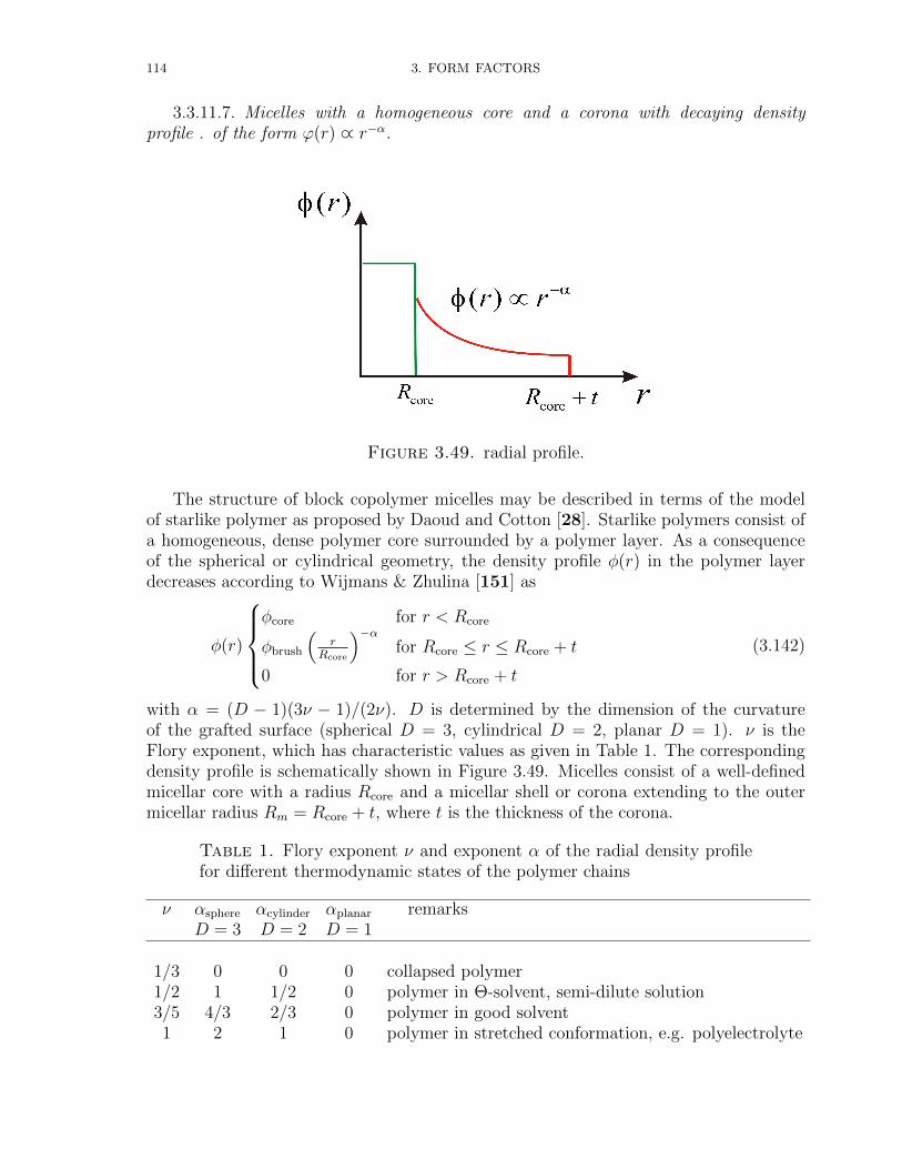
114 3. FORM FACTORS
3.3.11.7. Micelles with a homogeneous core and a corona with decaying densityprofile . of the form ϕ(r) ∝ r−α.
Figure 3.49. radial profile.
The structure of block copolymer micelles may be described in terms of the modelof starlike polymer as proposed by Daoud and Cotton [28]. Starlike polymers consist ofa homogeneous, dense polymer core surrounded by a polymer layer. As a consequenceof the spherical or cylindrical geometry, the density profile φ(r) in the polymer layerdecreases according to Wijmans & Zhulina [151] as
φ(r)
φcore for r < Rcore
φbrush
(r
Rcore
)−αfor Rcore ≤ r ≤ Rcore + t
0 for r > Rcore + t
(3.142)
with α = (D − 1)(3ν − 1)/(2ν). D is determined by the dimension of the curvatureof the grafted surface (spherical D = 3, cylindrical D = 2, planar D = 1). ν is theFlory exponent, which has characteristic values as given in Table 1. The correspondingdensity profile is schematically shown in Figure 3.49. Micelles consist of a well-definedmicellar core with a radius Rcore and a micellar shell or corona extending to the outermicellar radius Rm = Rcore + t, where t is the thickness of the corona.
Table 1. Flory exponent ν and exponent α of the radial density profilefor different thermodynamic states of the polymer chains
ν αsphere αcylinder αplanar remarksD = 3 D = 2 D = 1
1/3 0 0 0 collapsed polymer1/2 1 1/2 0 polymer in Θ-solvent, semi-dilute solution3/5 4/3 2/3 0 polymer in good solvent1 2 1 0 polymer in stretched conformation, e.g. polyelectrolyte
3.3. POLYMERS AND MICELLES 115
For a given radial profile according to eq. 3.142 the form factor of spherical micellecan be calculated by
FSPHERE =
∞∫0
2πr2φ(r)sin(qr)
qrdr (3.143)
In case of a rod-like micelle the form factor can be separated in two terms I(q) =PH(q)Pcs(q) as already in shown in eq. 3.135. The cross-term contribution to the scat-tering intensity is given by
Pcs(q) = F 2cs(q)
Fcs(q) =
∞∫0
2πrφ(r)J0(q) dr(3.144)
However, as it is more convenient here to formulate the scattering intensity in terms ofexcess scattering length of the block units in the core βcore and the corona βbrush like ineq. 3.74 the form factor is split into two parts, the form factor of the homogeneous coreFcore(q) and the form factor of the corona Fbrush(q). The overall scattering intensity I(q)is than given by
I(q) = N2aggβ
2coreF
2core(q) + 2N2
aggβcoreβcoronaFcore(q)Fcorona(q)
+Nagg(Nagg − 1)β2coronaF
2corona(q) +NaggPbrush(q)
(3.145)
The excess scattering length of a block in the corona and in the core, respectively,βbrush = Vbrush(ηbrush − ηsolv) and βcore = Vcore(ηcore − ηsolv) are defined in the same waythan in eq. 3.74. Vbrush and Vcore are the total volume of a block in the corona and inthe core. ηbrush and ηcore are the corresponding scattering length densities and ηsolv isthe scattering length density of the surrounding solvent. Fcore(q) is the form factor ofthe core and normalized to 1 for q = 0. Also the form factor of the corona Fcorona(q) andthe form factor of the local fluctuations in the corona originating from the individualchains Pbrush(q) are normalized to 1 for q = 0. Similar to section 3.3.11.1 models forspherical and rod-like shapes have been implemented which are described in the followingparagraphs.
3.3.11.8. spherical core:
Fcore(q, R) = 3sin(qR)− qR cos(qR)
(qR)3(3.146)
Fbrush(q, R, t) =1
Cnorm
Rcore+t∫Rcore
2πr2r−αsin(qr)
qrdr (3.147)
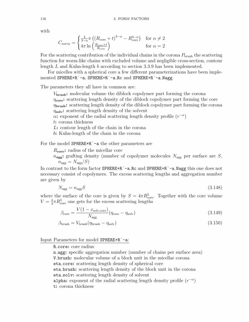
116 3. FORM FACTORS
with
Cnorm =
4
3−απ((Rcore + t)3−α −R3−α
core
)for α 6= 2
4π ln(Rcore+tRcore
)for α = 2
For the scattering contribution of the individual chains in the corona Pbrush the scatteringfunction for worm-like chains with excluded volume and negligible cross-section, contourlength L and Kuhn-length b according to section 3.3.9 has been implemented.
For micelles with a spherical core a few different parameterizations have been imple-mented SPHERE+Rˆ-a, SPHERE+Rˆ-a Rc and SPHERE+Rˆ-a Nagg.
The parameters they all have in common are:
Vbrush: molecular volume the diblock copolymer part forming the coronaηcore: scattering length density of the diblock copolymer part forming the coreηbrush: scattering length density of the diblock copolymer part forming the coronaηsolv: scattering length density of the solventα: exponent of the radial scattering length density profile (r−α)t: corona thicknessL: contour length of the chain in the coronab: Kuhn-length of the chain in the corona
For the model SPHERE+Rˆ-a the other parameters are
Rcore: radius of the micellar corenagg: grafting density (number of copolymer molecules Nagg per surface are S,nagg = Nagg/S)
In contrast to the form factor SPHERE+Rˆ-a Rc and SPHERE+Rˆ-a Nagg this one does notnecessary consist of copolymers. The excess scattering lengths and aggregation numberare given by
Nagg = naggS (3.148)
where the surface of the core is given by S = 4πR2core. Together with the core volume
V = 43πR3
core one gets for the excess scattering lengths
βcore =V (1− xsolv,core)
Nagg
(ηcore − ηsolv) (3.149)
βbrush = Vbrush(ηbrush − ηsolv) (3.150)
Input Parameters for model SPHERE+Rˆ-a:
R core: core radiusn agg: specific aggregation number (number of chains per surface area)V brush: molecular volume of a block unit in the micellar coronaeta core: scattering length density of spherical coreeta brush: scattering length density of the block unit in the coronaeta solv: scattering length density of solventalpha: exponent of the radial scattering length density profile (r−α)t: corona thickness
3.3. POLYMERS AND MICELLES 117
L: contour length of the chain in the coronab: Kuhn-length of the chain in the corona
118 3. FORM FACTORS
For the model SPHERE+Rˆ-a Rc the other parameters are
Rcore: core radiusVcore: molecular volume of single block unit in the micellar core
The excess scattering lengths and aggregation number for eq. 3.74 are given by
βcore = Vcore(ηcore − ηsolv) (3.151)
βbrush = Vbrush(ηbrush − ηsolv) (3.152)
Nagg = (1− xsolv,core)4
3πR3
core/Vcore (3.153)
Input Parameters for model SPHERE+Rˆ-a Rc:
R core: core radiusV core: molecular volume of single block unit in the micellar coreV brush: molecular volume of single block unit in the micellar coronaeta core: scattering length density of spherical coreeta brush: scattering length density of the block unit in the coronaeta solv: scattering length density of solventalpha: exponent of the radial scattering length density profile (r−α)t: corona thicknessL: contour length of the chain in the coronab: Kuhn-length of the chain in the corona
For the model SPHERE+Rˆ-a Nagg the other parameters are
Nagg: aggregation numberVcore: molecular volume of single block unit in the micellar core
The excess scattering lengths and the core radius Rcore needed for eq. 3.74 are given by
βcore = Vcore(ηcore − ηsolv) (3.154)
βbrush = Vbrush(ηbrush − ηsolv) (3.155)
Rcore =
(NaggVcore
1− xsolv,core
3
4π
)1/3
(3.156)
Input Parameters for model SPHERE+Rˆ-a Nagg:
N agg: aggregation numberV core: molecular volume of single block unit in the micellar coreV brush: molecular volume of single block unit in the micellar coronaeta core: scattering length density of spherical coreeta brush: scattering length density of the block unit in the coronaeta solv: scattering length density of solventalpha: exponent of the radial scattering length density profile (r−α)t: corona thicknessL: contour length of the chain in the coronab: Kuhn-length of the chain in the corona
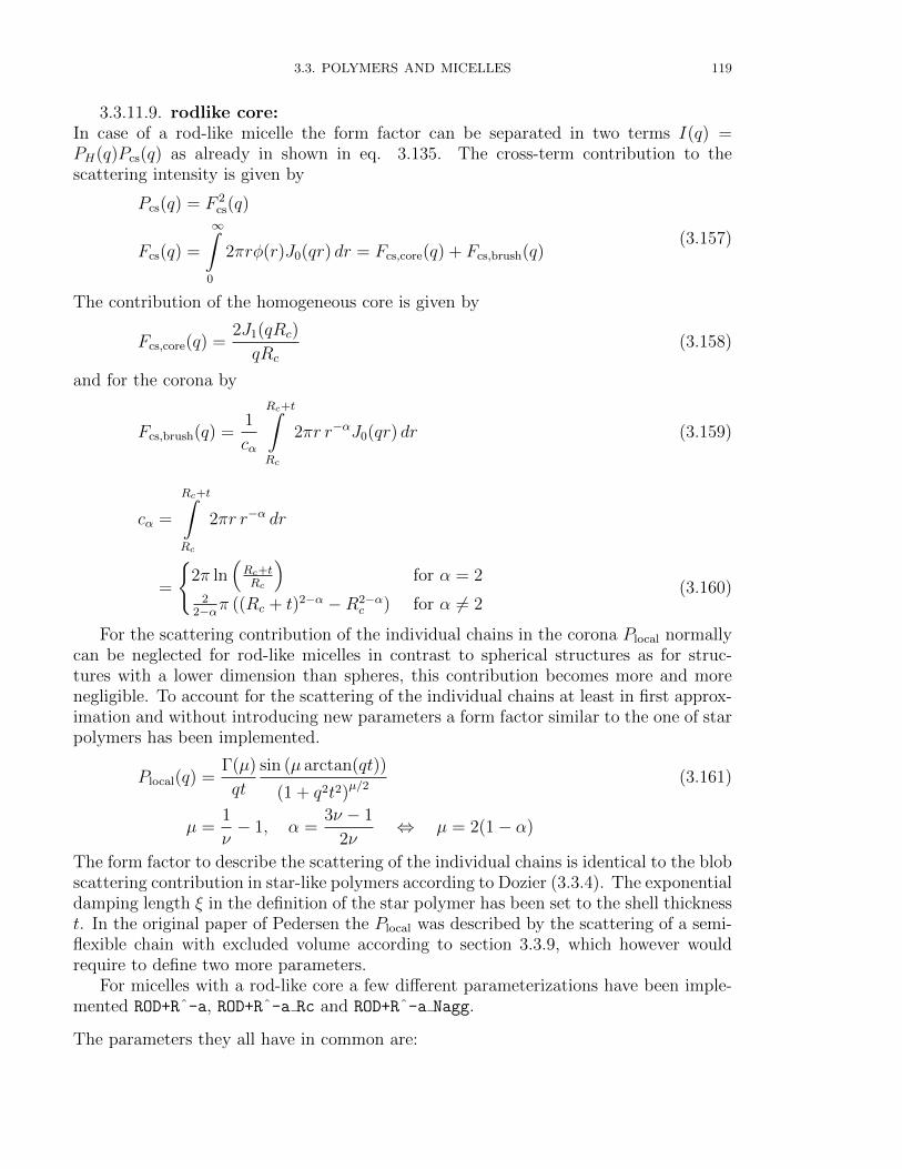
3.3. POLYMERS AND MICELLES 119
3.3.11.9. rodlike core:In case of a rod-like micelle the form factor can be separated in two terms I(q) =PH(q)Pcs(q) as already in shown in eq. 3.135. The cross-term contribution to thescattering intensity is given by
Pcs(q) = F 2cs(q)
Fcs(q) =
∞∫0
2πrφ(r)J0(qr) dr = Fcs,core(q) + Fcs,brush(q)(3.157)
The contribution of the homogeneous core is given by
Fcs,core(q) =2J1(qRc)
qRc
(3.158)
and for the corona by
Fcs,brush(q) =1
cα
Rc+t∫Rc
2πr r−αJ0(qr) dr (3.159)
cα =
Rc+t∫Rc
2πr r−α dr
=
2π ln
(Rc+tRc
)for α = 2
22−απ ((Rc + t)2−α −R2−α
c ) for α 6= 2(3.160)
For the scattering contribution of the individual chains in the corona Plocal normallycan be neglected for rod-like micelles in contrast to spherical structures as for struc-tures with a lower dimension than spheres, this contribution becomes more and morenegligible. To account for the scattering of the individual chains at least in first approx-imation and without introducing new parameters a form factor similar to the one of starpolymers has been implemented.
Plocal(q) =Γ(µ)
qt
sin (µ arctan(qt))
(1 + q2t2)µ/2(3.161)
µ =1
ν− 1, α =
3ν − 1
2ν⇔ µ = 2(1− α)
The form factor to describe the scattering of the individual chains is identical to the blobscattering contribution in star-like polymers according to Dozier (3.3.4). The exponentialdamping length ξ in the definition of the star polymer has been set to the shell thicknesst. In the original paper of Pedersen the Plocal was described by the scattering of a semi-flexible chain with excluded volume according to section 3.3.9, which however wouldrequire to define two more parameters.
For micelles with a rod-like core a few different parameterizations have been imple-mented ROD+Rˆ-a, ROD+Rˆ-a Rc and ROD+Rˆ-a Nagg.
The parameters they all have in common are:
120 3. FORM FACTORS
Vbrush: molecular volume the diblock copolymer part forming the coronaηcore: scattering length density of the diblock copolymer part forming the coreηbrush: scattering length density of the diblock copolymer part forming the coronaηsolv: scattering length density of the solventxsolv,core: amount of solvent in the coreα: exponent of the radial scattering length density profile (r−α)t: corona thicknessH: height of the cylinder
For the model ROD+Rˆ-a the other parameters are
Rcore: radius of the micellar corenagg: grafting density (number of copolymer molecules Nagg per surface are S,nagg = Nagg/S)
In contrast to the form factor ROD+Rˆ-a Rc and ROD+Rˆ-a Nagg this one does not nec-essary consist of copolymers. The excess scattering lengths and aggregation number aregiven by
Nagg = naggS (3.162)
where the surface of the core is given by S = 2πRcoreH. Together with the core volumeV = πR2
coreH one gets for the excess scattering lengths
βcore =Vcore(1− xsolv,core)
Nagg
(ηcore − ηsolv) (3.163)
βbrush = Vbrush(ηbrush − ηsolv) (3.164)
Input Parameters for model ROD+Rˆ-a:
R core: core radiusn agg: specific aggregation number (number of chains per surface area)V brush: molecular volume of a block unit in the micellar coronaeta core: scattering length density of spherical coreeta brush: scattering length density of the block unit in the coronaeta solv: scattering length density of solventxsolv core: amount of solvent in the corealpha: exponent of the radial scattering length density profile (r−α)t: corona thicknessH: rod height
For the model ROD+Rˆ-a Rc the other parameters are
Rcore: core radiusVcore: molecular volume of single block unit in the micellar core

3.3. POLYMERS AND MICELLES 121
The excess scattering lengths and aggregation number for eq. 3.74 are given by
βcore = Vcore(ηcore − ηsolv) (3.165)
βbrush = Vbrush(ηbrush − ηsolv) (3.166)
Nagg = 2πR2coreH
1− xsolv,core
Vcore
(3.167)
Input Parameters for model ROD+Rˆ-a Rc:
R core: core radiusV core: molecular volume of single block unit in the micellar coreV brush: molecular volume of single block unit in the micellar coronaeta core: scattering length density of spherical coreeta brush: scattering length density of the block unit in the coronaeta solv: scattering length density of solventxsolv core: amount of solvent in the corealpha: exponent of the radial scattering length density profile (r−α)t: corona thicknessH: rod height
For the model ROD+Rˆ-a Nagg the other parameters are
nagg: specific aggregation number, aggregation number per surface areaVcore: molecular volume of single block unit in the micellar core
The excess scattering lengths and the core radius Rcore needed for eq. 3.74 are given by
βcore = Vcore(ηcore − ηsolv) (3.168)
βbrush = Vbrush(ηbrush − ηsolv) (3.169)
Rcore =2nagg Vcore
1− xsolv,core
(3.170)
Input Parameters for model ROD+Rˆ-a nagg:
n agg: specific aggregation number (number of chains per surface area)V core: molecular volume of single block unit in the micellar coreV brush: molecular volume of single block unit in the micellar coronaeta core: scattering length density of spherical coreeta brush: scattering length density of the block unit in the coronaeta solv: scattering length density of solventxsolv core: amount of solvent in the corealpha: exponent of the radial scattering length density profile (r−α)t: corona thicknessH: rod height
REFERENCES:[28, 39, 100, 151]
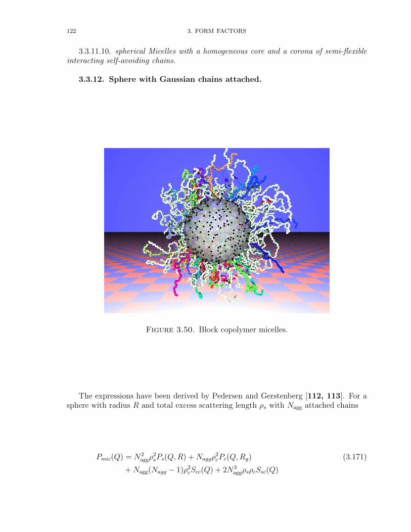
122 3. FORM FACTORS
3.3.11.10. spherical Micelles with a homogeneous core and a corona of semi-flexibleinteracting self-avoiding chains.
3.3.12. Sphere with Gaussian chains attached.
Figure 3.50. Block copolymer micelles.
The expressions have been derived by Pedersen and Gerstenberg [112, 113]. For asphere with radius R and total excess scattering length ρs with Nagg attached chains
Pmic(Q) = N2aggρ
2sPs(Q,R) +Naggρ
2cPc(Q,Rg) (3.171)
+Nagg(Nagg − 1)ρ2cScc(Q) + 2N2
aggρsρcSsc(Q)
3.3. POLYMERS AND MICELLES 123
with:
Ps = Φ2(Q,R) (3.172)
Φ(Q,R) = 3sin(QR)−QR cos(QR)
(QR)3(3.173)
Pc(Q,Rg) = 2exp(−x)− 1 + x
x2(3.174)
x = R2gQ
2 (3.175)
Ψ(Q,Rg) =1− exp(−x)
x(3.176)
Scc(Q) = Ψ2(Q,Rg)
(sin(Q(R + d Rg))
Q(R + dRg)
)2
(3.177)
Ssc(Q) = Ψ(Q,Rg)Φ(QRg)sin(Q(R + dRg))
Q(R + dRg)(3.178)
where Rg is the root-mean-square radius of gyration of a chain. ρc is the total excessscattering length of a single chain. Non-penetrating of the chains into the core region ismimicked by d ≈ 1 for R Rg.
Input Parameters for model SphereWithGaussChains:
R: radius of core RRg: gyration radius of chain Rg
d: for non-penetration of the chains into the core region d ≈ 1.Nagg: aggregation number Nagg
rc: excess scattering length of a block in the chains ρcrs: excess scattering length of a block in the core ρs
124 3. FORM FACTORS
3.3.13. Sphere with Gaussian chains attached (block copolymer micelle).
This form factor is the same than for SphereWithGaussChains. It has only beenslightly re-parametrised. Instead of the core radius R and excess scattering lengths ρsand ρc the volumes Vpolym,c and Vpolym,sh of the block units building the core and the shellare required together with the corresponding scattering length densities ηpoly,c, ηpoly,sh
and that one of the solvent ηsolv. Furthermore xsolv,c is the amount of solvent in the corewhich takes account for a possible swelling of the core. These parameters allow one tocalculate the core radius and excess scattering lengths by
R =
(∣∣∣∣NaggVpolym,c
1− xsolv,c
∣∣∣∣ 3
4π
)1/3
(3.179)
ρs = Vpolym,c (ηpoly,c − ηsolv) (3.180)
ρc = Vpolym,sh (ηpoly,sh − ηsolv) (3.181)
The volumes Vpolym,c and Vpolym,sh can be calculated by knowing the molecularweights5 of the block units of the polymer in the core Mpolym,c and in the shell Mpolym,sh
together with their bulk mass densities ρpolym,c and ρpolym,sh. The volumes are then givenby
Vpolym,c =Mpolym,c
Na ρpolym,c
and Vpolym,sh =Mpolym,sh
Na ρpolym,sh
(3.182)
whereby Na is Avogadro’s constant6. The units of the block units has to be supplied inunits corresponding to the scattering vector Q, i.e. in nm3 in case Q is given in nm−1
or in A3 in case Q is given in A−1.
Input Parameters for model BlockCopolymerMicelle:
Vpolym c: volume of a single block unit of the chains in the core Vpolym,c, it shouldbe given in units of nm3 in case Q is given in nm−1 and in units of A3 in caseQ is given in A−1.
xsolv c: amount of solvent in the core (xsolv,c 6= 1)Vpolym sh: volume of a single block unit of the chains in the shell Vpolym,sh, it
should be given in units of nm3 in case Q is given in nm−1 and in units of A3
in case Q is given in A−1.eta poly c: scattering length density of the block units in the core ηc
eta poly sh: scattering length density of the block units in the chains ηsh
eta solv: scattering length density of the solvent ηsolv
Nagg: aggregation number Nagg
Rg: gyration radius of chain Rg
d: for non-penetration of the chains into the core region d ≈ 1.
5u = 1.66053886× 10⁻²⁷ kg6Na = 6.0221415× 10²³mol−1
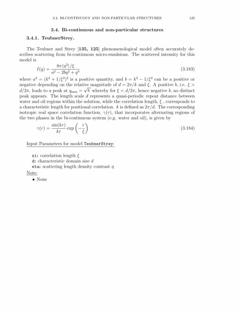
3.4. BI-CONTINUOUS AND NON-PARTICULAR STRUCTURES 125
3.4. Bi-continuous and non-particular structures
3.4.1. TeubnerStrey.
The Teubner and Strey [135, 125] phenomenological model often accurately de-scribes scattering from bi-continuous micro-emulsions. The scattered intensity for thismodel is
I(q) =8π〈η2〉/ξ
a2 − 2bq2 + q4(3.183)
where a2 = (k2 + 1/ξ2)2 is a positive quantity, and b = k2 − 1/ξ2 can be a positive ornegative depending on the relative magnitude of d = 2π/k and ξ. A positive b, i.e. ξ >
d/2π, leads to a peak at qmax =√b whereby for ξ < d/2π, hence negative b, no distinct
peak appears. The length scale d represents a quasi-periodic repeat distance betweenwater and oil regions within the solution, while the correlation length, ξ , corresponds toa characteristic length for positional correlation. k is defined as 2π/d. The correspondingisotropic real space correlation function, γ(r), that incorporates alternating regions ofthe two phases in the bi-continuous system (e.g. water and oil), is given by
γ(r) =sin(kr)
krexp
(−rξ
)(3.184)
Input Parameters for model TeubnerStrey:
xi: correlation length ξd: characteristic domain size deta: scattering length density contrast η
Note:
• None
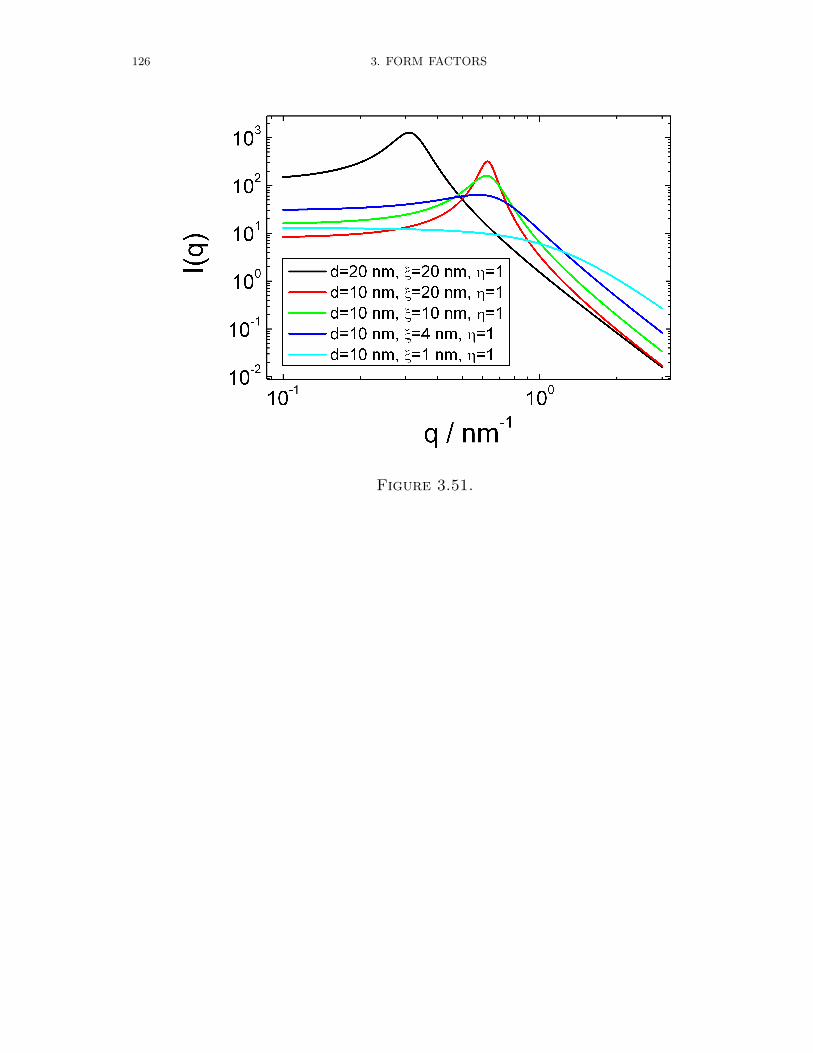
126 3. FORM FACTORS
Figure 3.51.
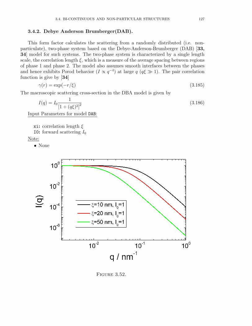
3.4. BI-CONTINUOUS AND NON-PARTICULAR STRUCTURES 127
3.4.2. Debye Anderson Brumberger(DAB).
This form factor calculates the scattering from a randomly distributed (i.e. non-particulate), two-phase system based on the Debye-Anderson-Brumberger (DAB) [33,34] model for such systems. The two-phase system is characterized by a single lengthscale, the correlation length ξ, which is a measure of the average spacing between regionsof phase 1 and phase 2. The model also assumes smooth interfaces between the phasesand hence exhibits Porod behavior (I ∝ q−4) at large q (qξ 1). The pair correlationfunction is give by [34]
γ(r) = exp(−r/ξ) (3.185)
The macroscopic scattering cross-section in the DBA model is given by
I(q) = I01
[1 + (qξ)2]2(3.186)
Input Parameters for model DAB:
xi: correlation length ξI0: forward scattering I0
Note:
• None
Figure 3.52.
128 3. FORM FACTORS
3.4.3. Spinodal.
Figure 3.53. Schematic representation of a phase separation scheme re-sulting in a connected globule structure.
Spinodal decomposing systems show a characteristic small angle scattering signalwith a correlation peak at some scattering value qmax. The scattering curve I(q) can beapproximated by
I(q) = Imax(1 + γ/2)x2
γ/2 + x2+γ(3.187)
according to Furukawa [45], where x = q/qmax. The position of the correlation peak atqmax contain information about the size of the structures, which scatter. The exponentγ is equal to γ = D + 1 for off-critical mixtures and γ = 2D for critical concentrationmixtures, whereby D is the dimensionality of the system.
Input Parameters for model Spinodal:
Qmax: peak maximum qmax
gamma: exponent γImax: scattering intensity at peak position Imax
Note:
• None

3.4. BI-CONTINUOUS AND NON-PARTICULAR STRUCTURES 129
Figure 3.54.
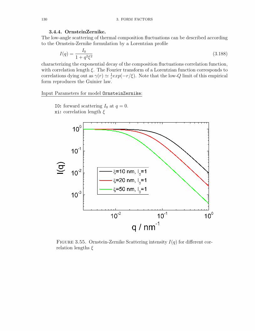
130 3. FORM FACTORS
3.4.4. OrnsteinZernike.The low-angle scattering of thermal composition fluctuations can be described accordingto the Ornstein-Zernike formulation by a Lorentzian profile
I(q) =I0
1 + q2ξ2(3.188)
characterizing the exponential decay of the composition fluctuations correlation function,with correlation length ξ. The Fourier transform of a Lorentzian function corresponds tocorrelations dying out as γ(r) ' 1
rexp(−r/ξ). Note that the low-Q limit of this empirical
form reproduces the Guinier law.
Input Parameters for model OrnsteinZernike:
I0: forward scattering I0 at q = 0.xi: correlation length ξ
Figure 3.55. Ornstein-Zernike Scattering intensity I(q) for different cor-relation lengths ξ

3.4. BI-CONTINUOUS AND NON-PARTICULAR STRUCTURES 131
3.4.5. BroadPeak.Many SANS spectra are characterized by a broad peak even though they are from amor-phous soft materials. The d-spacing corresponding to the broad peak is a characteristicdistance between the scattering inhomogeneities (such as in lamellar, cylindrical, orspherical morphologies or for bicontinuous structures). The following simple functionalform reproduces the broad peak feature:
I(q) =I0
1 + (|q − q0|ξ)m(3.189)
Here the peak position is related to the d-spacing as q0 = 2π/d. Soft systems thatshow a SANS peak include copolymers, polyelectrolytes, multiphase systems, layeredstructures, etc.
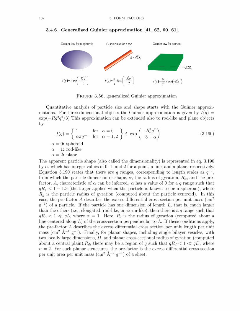
132 3. FORM FACTORS
3.4.6. Generalized Guinier approximation [41, 62, 60, 61].
Figure 3.56. generalized Guinier approximation
Quantitative analysis of particle size and shape starts with the Guinier approxi-mations. For three-dimensional objects the Guinier approximation is given by I(q) =exp(−Rg2q2/3) This approximation can be extended also to rod-like and plane objectsby
I(q) =
1 for α = 0απq−α for α = 1, 2
A exp
(−R
2αq
2
3− α
)(3.190)
α = 0: spheroidα = 1: rod-likeα = 2: plane
The apparent particle shape (also called the dimensionality) is represented in eq. 3.190by α, which has integer values of 0, 1, and 2 for a point, a line, and a plane, respectively.Equation 3.190 states that there are q ranges, corresponding to length scales as q−1,from which the particle dimension or shape, α, the radius of gyration, Rα, and the pre-factor, A, characteristic of α can be inferred. α has a value of 0 for a q range such thatqRg < 1 − 1.3 (the larger applies when the particle is known to be a spheroid), whereRg is the particle radius of gyration (computed about the particle centroid). In thiscase, the pre-factor A describes the excess differential cross-section per unit mass (cm2
g−1) of a particle. If the particle has one dimension of length L, that is, much largerthan the others (i.e., elongated, rod-like, or worm-like), then there is a q range such thatqRc < 1 qL, where α = 1. Here, Rc is the radius of gyration (computed about aline centered along L) of the cross-section perpendicular to L. If these conditions apply,the pre-factor A describes the excess differential cross section per unit length per unitmass (cm2 A−1 g−1). Finally, for planar shapes, including single bilayer vesicles, withtwo locally large dimensions, D, and planar cross-sectional radius of gyration (computedabout a central plain),Rd, there may be a region of q such that qRd < 1 qD, whereα = 2. For such planar structures, the pre-factor is the excess differential cross-sectionper unit area per unit mass (cm2 A−2 g−1) of a sheet.
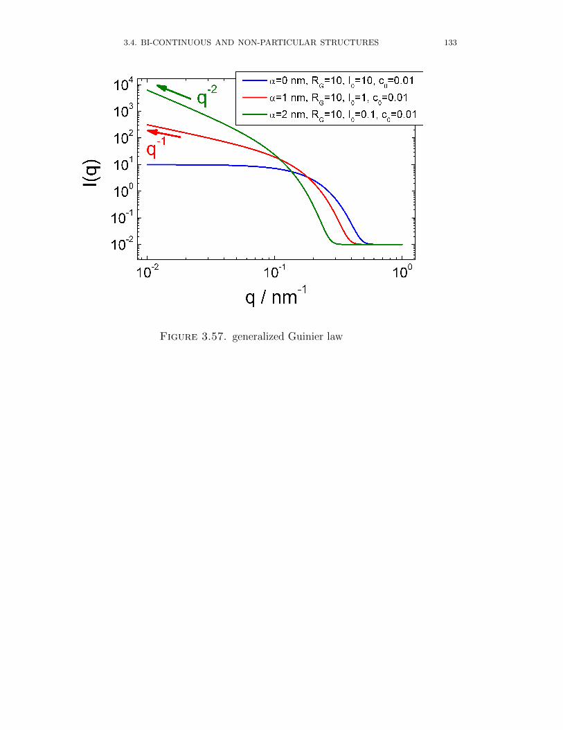
3.4. BI-CONTINUOUS AND NON-PARTICULAR STRUCTURES 133
Figure 3.57. generalized Guinier law
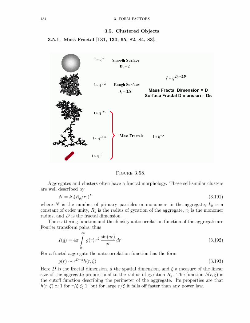
134 3. FORM FACTORS
3.5. Clustered Objects
3.5.1. Mass Fractal [131, 130, 65, 82, 84, 83].
Figure 3.58.
Aggregates and clusters often have a fractal morphology. These self-similar clustersare well described by
N = k0(Rg/r0)D (3.191)
where N is the number of primary particles or monomers in the aggregate, k0 is aconstant of order unity, Rg is the radius of gyration of the aggregate, r0 is the monomerradius, and D is the fractal dimension.
The scattering function and the density autocorrelation function of the aggregate areFourier transform pairs; thus
I(q) = 4π
∞∫0
g(r) r2 sin(qr)
qrdr (3.192)
For a fractal aggregate the autocorrelation function has the form
g(r) ∼ rD−dh(r, ξ) (3.193)
Here D is the fractal dimension, d the spatial dimension, and ξ a measure of the linearsize of the aggregate proportional to the radius of gyration Rg. The function h(r, ξ) isthe cutoff function describing the perimeter of the aggregate. Its properties are thath(r, ξ) ' 1 for r/ξ . 1, but for large r/ξ it falls off faster than any power law.
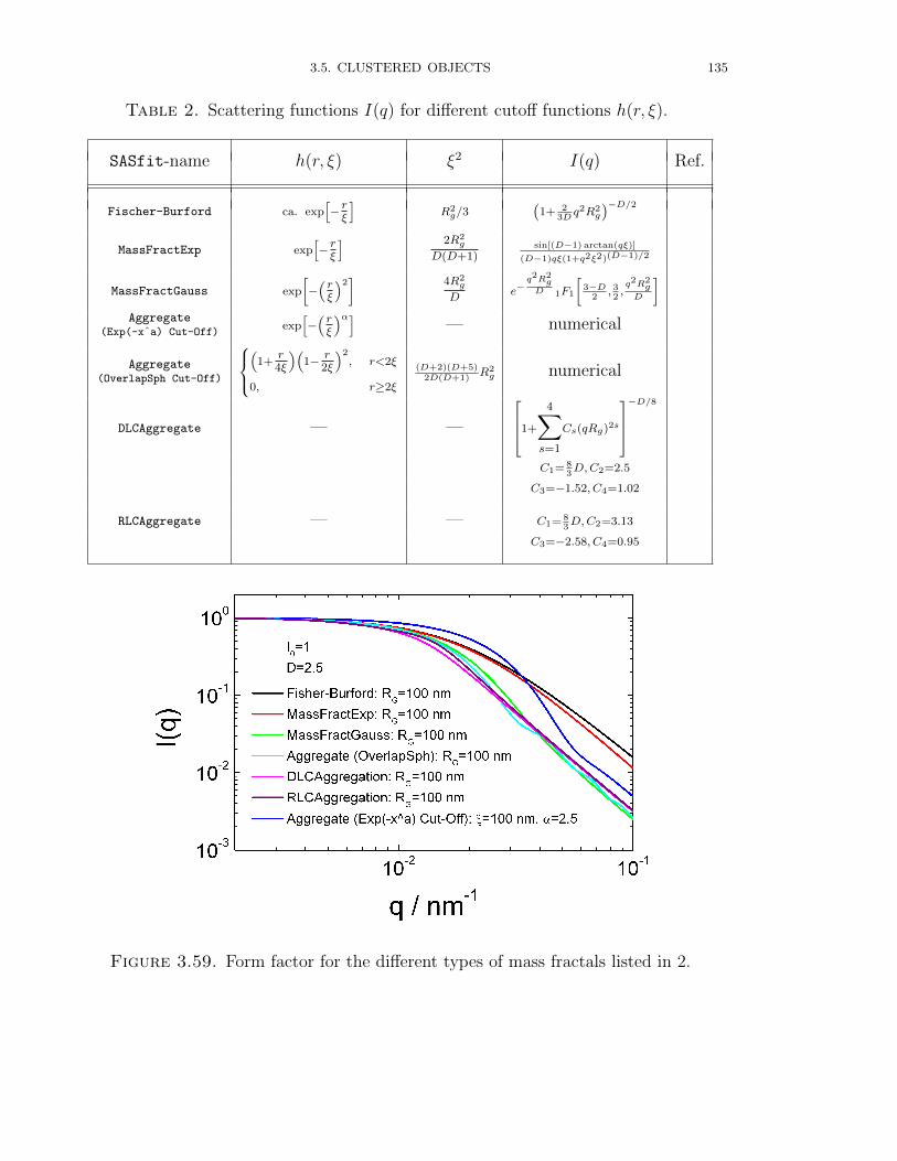
3.5. CLUSTERED OBJECTS 135
Table 2. Scattering functions I(q) for different cutoff functions h(r, ξ).
SASfit-name h(r, ξ) ξ2 I(q) Ref.
Fischer-Burford ca. exp[− rξ
]R2g/3 (1+ 2
3Dq2R2
g)−D/2
MassFractExp exp[− rξ
] 2R2g
D(D+1)sin[(D−1) arctan(qξ)]
(D−1)qξ(1+q2ξ2)(D−1)/2
MassFractGauss exp
[−(rξ
)2]
4R2g
De−
q2R2g
D 1F1
[3−D
2, 32,q2R2
gD
]Aggregate
(Exp(-xˆa) Cut-Off)exp[−(rξ
)α]— numerical
Aggregate(OverlapSph Cut-Off)
(
1+r4ξ
)(1− r
2ξ
)2, r<2ξ
0, r≥2ξ
(D+2)(D+5)2D(D+1)
R2g numerical
DLCAggregate — —
1+
4∑s=1
Cs(qRg)2s
−D/8
C1= 83D,C2=2.5
C3=−1.52, C4=1.02
RLCAggregate — — C1= 83D,C2=3.13
C3=−2.58, C4=0.95
Figure 3.59. Form factor for the different types of mass fractals listed in 2.
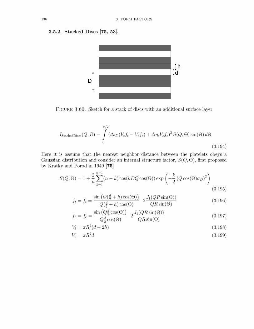
136 3. FORM FACTORS
3.5.2. Stacked Discs [75, 53].
Figure 3.60. Sketch for a stack of discs with an additional surface layer
IStackedDiscs(Q,R) =
π/2∫0
(∆ηl (Vtft − Vcfc) + ∆ηcVcfc)2 S(Q,Θ) sin(Θ) dΘ
(3.194)
Here it is assume that the nearest neighbor distance between the platelets obeys aGaussian distribution and consider an internal structure factor, S(Q,Θ), first proposedby Kratky and Porod in 1949 [75]
S(Q,Θ) = 1 +2
n
n−1∑k=1
(n− k) cos(kDQ cos(Θ)) exp
(−k
2(Q cos(Θ)σD)2
)(3.195)
ft = ft =sin(Q(d
2+ h) cos(Θ)
)Q(d
2+ h) cos(Θ)
2J1(QR sin(Θ))
QR sin(Θ)(3.196)
fc = fc =sin(Qd
2cos(Θ)
)Qd
2cos(Θ)
2J1(QR sin(Θ))
QR sin(Θ)(3.197)
Vt = πR2(d+ 2h) (3.198)
Vc = πR2d (3.199)

3.5. CLUSTERED OBJECTS 137
Figure 3.61. Scattering Intensity for a stack of discs with a layer.
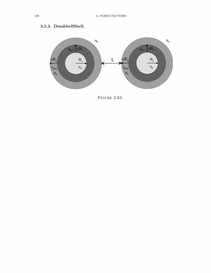
138 3. FORM FACTORS
3.5.3. DumbbellShell.
Figure 3.62.
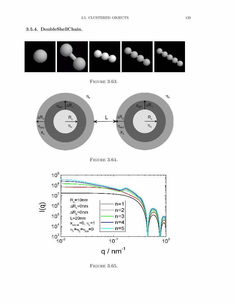
3.5. CLUSTERED OBJECTS 139
3.5.4. DoubleShellChain.
Figure 3.63.
Figure 3.64.
Figure 3.65.
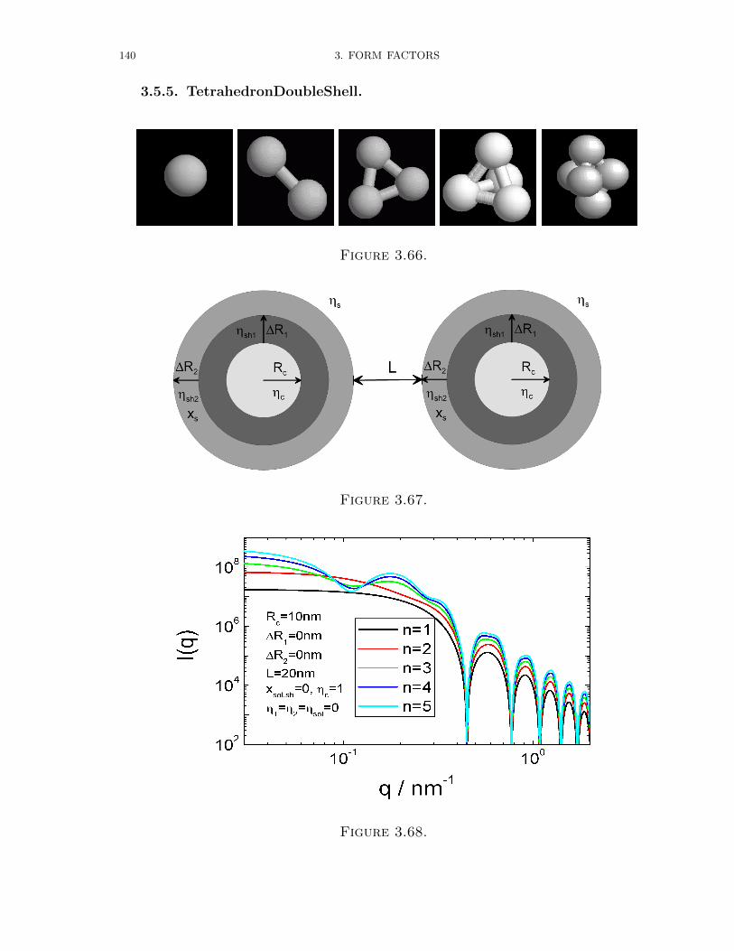
140 3. FORM FACTORS
3.5.5. TetrahedronDoubleShell.
Figure 3.66.
Figure 3.67.
Figure 3.68.
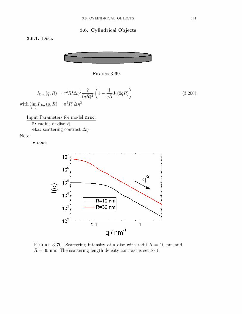
3.6. CYLINDRICAL OBJECTS 141
3.6. Cylindrical Objects
3.6.1. Disc.
Figure 3.69.
IDisc(q, R) = π2R4∆η2 2
(qR)2
(1− 1
qRJ1(2qR)
)(3.200)
with limq=0
IDisc(q, R) = π2R4∆η2
Input Parameters for model Disc:
R: radius of disc Reta: scattering contrast ∆η
Note:
• none
Figure 3.70. Scattering intensity of a disc with radii R = 10 nm andR = 30 nm. The scattering length density contrast is set to 1.
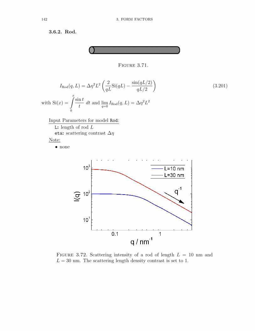
142 3. FORM FACTORS
3.6.2. Rod.
Figure 3.71.
IRod(q, L) = ∆η2L2
(2
qLSi(qL)− sin(qL/2)
qL/2
)(3.201)
with Si(x) =
x∫0
sin t
tdt and lim
q=0IRod(q, L) = ∆η2L2
Input Parameters for model Rod:
L: length of rod Leta: scattering contrast ∆η
Note:
• none
Figure 3.72. Scattering intensity of a rod of length L = 10 nm andL = 30 nm. The scattering length density contrast is set to 1.
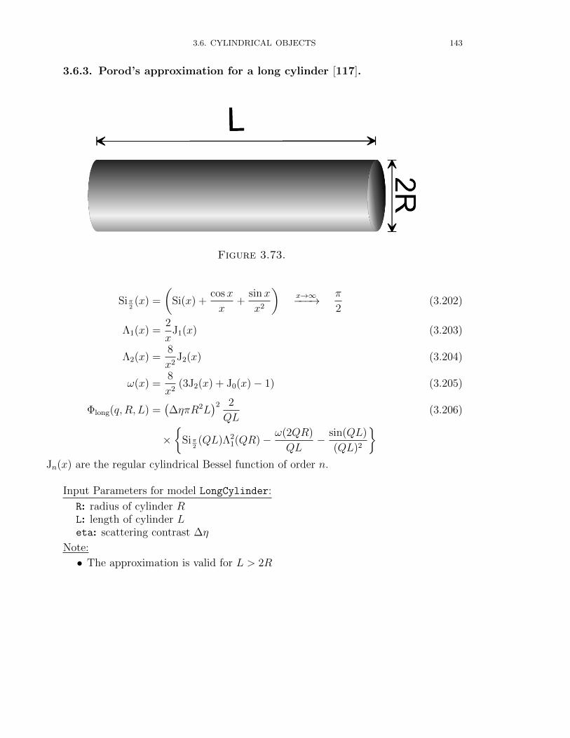
3.6. CYLINDRICAL OBJECTS 143
3.6.3. Porod’s approximation for a long cylinder [117].
Figure 3.73.
Siπ2(x) =
(Si(x) +
cosx
x+
sinx
x2
)x→∞−−−→ π
2(3.202)
Λ1(x) =2
xJ1(x) (3.203)
Λ2(x) =8
x2J2(x) (3.204)
ω(x) =8
x2(3J2(x) + J0(x)− 1) (3.205)
Φlong(q, R, L) =(∆ηπR2L
)2 2
QL(3.206)
×
Siπ2(QL)Λ2
1(QR)− ω(2QR)
QL− sin(QL)
(QL)2
Jn(x) are the regular cylindrical Bessel function of order n.
Input Parameters for model LongCylinder:
R: radius of cylinder RL: length of cylinder Leta: scattering contrast ∆η
Note:
• The approximation is valid for L > 2R
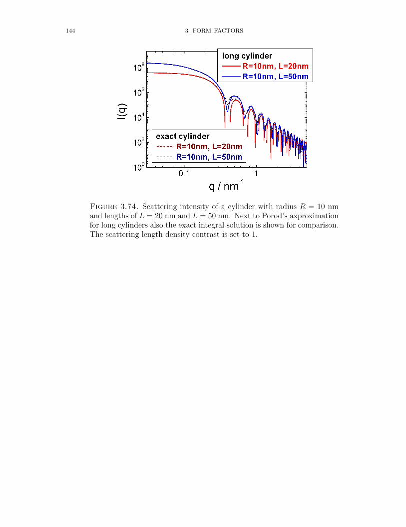
144 3. FORM FACTORS
Figure 3.74. Scattering intensity of a cylinder with radius R = 10 nmand lengths of L = 20 nm and L = 50 nm. Next to Porod’s axproximationfor long cylinders also the exact integral solution is shown for comparison.The scattering length density contrast is set to 1.
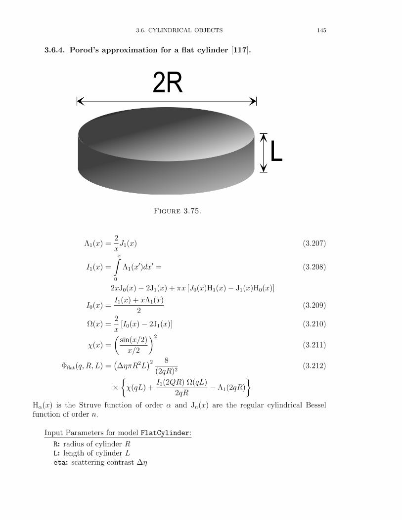
3.6. CYLINDRICAL OBJECTS 145
3.6.4. Porod’s approximation for a flat cylinder [117].
Figure 3.75.
Λ1(x) =2
xJ1(x) (3.207)
I1(x) =
x∫0
Λ1(x′)dx′ = (3.208)
2xJ0(x)− 2J1(x) + πx [J0(x)H1(x)− J1(x)H0(x)]
I0(x) =I1(x) + xΛ1(x)
2(3.209)
Ω(x) =2
x[I0(x)− 2J1(x)] (3.210)
χ(x) =
(sin(x/2)
x/2
)2
(3.211)
Φflat(q, R, L) =(∆ηπR2L
)2 8
(2qR)2(3.212)
×χ(qL) +
I1(2QR) Ω(qL)
2qR− Λ1(2qR)
Hα(x) is the Struve function of order α and Jn(x) are the regular cylindrical Besselfunction of order n.
Input Parameters for model FlatCylinder:
R: radius of cylinder RL: length of cylinder Leta: scattering contrast ∆η

146 3. FORM FACTORS
Note:
• The approximation is valid for L < 2R
Figure 3.76. Scattering intensity of a cylinder with radius R = 10 nmand lengths of L = 2 nm and L = 20 nm. Next to Porod’s axproximationfor flat cylinders also the exact integral solution is shown for comparison.The scattering length density contrast is set to 1.
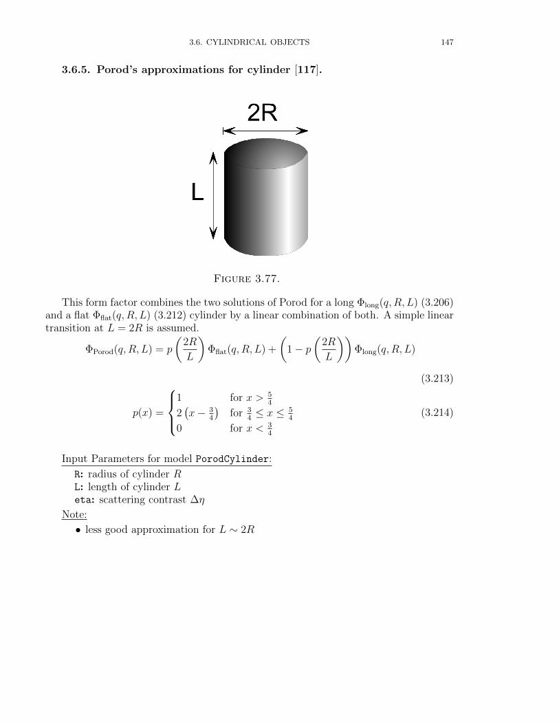
3.6. CYLINDRICAL OBJECTS 147
3.6.5. Porod’s approximations for cylinder [117].
Figure 3.77.
This form factor combines the two solutions of Porod for a long Φlong(q, R, L) (3.206)and a flat Φflat(q, R, L) (3.212) cylinder by a linear combination of both. A simple lineartransition at L = 2R is assumed.
ΦPorod(q, R, L) = p
(2R
L
)Φflat(q, R, L) +
(1− p
(2R
L
))Φlong(q, R, L)
(3.213)
p(x) =
1 for x > 5
4
2(x− 3
4
)for 3
4≤ x ≤ 5
4
0 for x < 34
(3.214)
Input Parameters for model PorodCylinder:
R: radius of cylinder RL: length of cylinder Leta: scattering contrast ∆η
Note:
• less good approximation for L ∼ 2R

148 3. FORM FACTORS
Figure 3.78. Scattering intensity of a cylinder with radius R = 10 nmand lengths of L = 2 nm, L = 20 nm, and L = 50 nm. Next to Porod’saxproximation for a cylinders also the exact integral solution is shown forcomparison. The scattering length density contrast is set to 1.

3.6. CYLINDRICAL OBJECTS 149
3.6.6. Cylinder of length L, radius R and scattering contrast ∆η.
Figure 3.79.
Icyl = 16(πR2L)2∆η2
1∫0
(J1
(QR√
1− x2)
sin(QLx/2)
Q2R√
1− x2 Lx
)2
dx (3.215)
Input Parameters for model Cylinder:
R: radius of cylinder RL: length of cylinder Leta: scattering contrast ∆η
Note:
• None
Figure 3.80. Scattering intensity of a cylinder for different radii radiusR nm and lengths L. The scattering length density contrast is set to 1.

150 3. FORM FACTORS
3.6.7. Random oriented cylindrical shell with circular cross-section.
Figure 3.81. cylindrical shell with circular cross-section
To different versions for a random oriented cylindrical shell with a circular cross-section has been implemented. One without CylShell1 and one with CylShell2 cappedends. For very long cylinders a faster approximation for the uncapped version can beused LongCylShell
KCyl(Q,∆η,R, L, x) = 2πR2L∆ηJ1
(QR√
1− x2)
QR√
1− x2
sin(QLx/2)
QLx/2(3.216)
ICylShell1 =
1∫0
(KCyl (Q, ηcore − ηshell, R, L, x) (3.217)
+KCyl (Q, ηshell − ηsolv, R + ∆R,L, x)
)2
dx
ICylShell2 =
1∫0
(KCyl (Q, ηcore − ηshell, R, L, x) (3.218)
+KCyl (Q, ηshell − ηsolv, R + ∆R,L+ 2∆R, x)
)2
dx
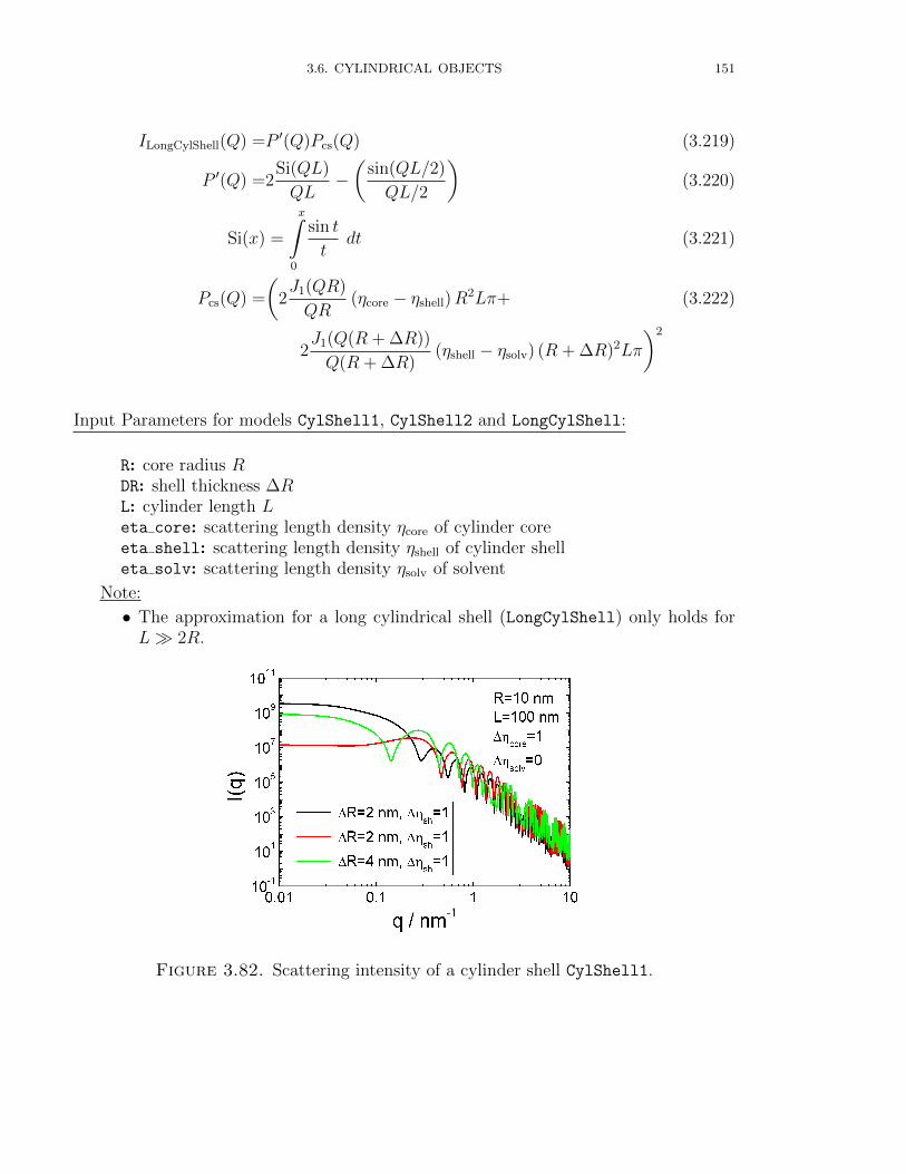
3.6. CYLINDRICAL OBJECTS 151
ILongCylShell(Q) =P ′(Q)Pcs(Q) (3.219)
P ′(Q) =2Si(QL)
QL−(
sin(QL/2)
QL/2
)(3.220)
Si(x) =
x∫0
sin t
tdt (3.221)
Pcs(Q) =
(2J1(QR)
QR(ηcore − ηshell)R
2Lπ+ (3.222)
2J1(Q(R + ∆R))
Q(R + ∆R)(ηshell − ηsolv) (R + ∆R)2Lπ
)2
Input Parameters for models CylShell1, CylShell2 and LongCylShell:
R: core radius RDR: shell thickness ∆RL: cylinder length Leta core: scattering length density ηcore of cylinder coreeta shell: scattering length density ηshell of cylinder shelleta solv: scattering length density ηsolv of solvent
Note:
• The approximation for a long cylindrical shell (LongCylShell) only holds forL 2R.
Figure 3.82. Scattering intensity of a cylinder shell CylShell1.
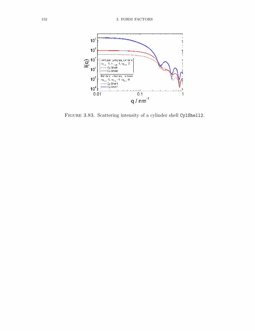
152 3. FORM FACTORS
Figure 3.83. Scattering intensity of a cylinder shell CylShell2.
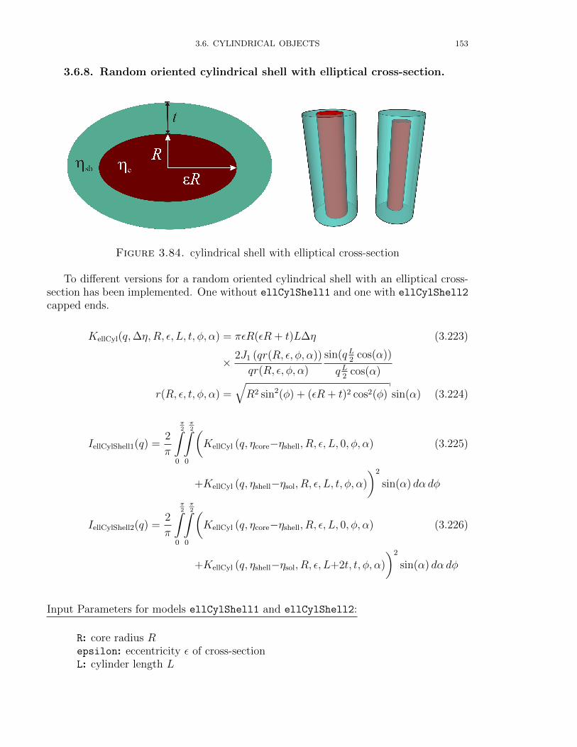
3.6. CYLINDRICAL OBJECTS 153
3.6.8. Random oriented cylindrical shell with elliptical cross-section.
Figure 3.84. cylindrical shell with elliptical cross-section
To different versions for a random oriented cylindrical shell with an elliptical cross-section has been implemented. One without ellCylShell1 and one with ellCylShell2
capped ends.
KellCyl(q,∆η,R, ε, L, t, φ, α) = πεR(εR + t)L∆η (3.223)
× 2J1 (qr(R, ε, φ, α))
qr(R, ε, φ, α)
sin(qL2
cos(α))
qL2
cos(α)
r(R, ε, t, φ, α) =√R2 sin2(φ) + (εR + t)2 cos2(φ) sin(α) (3.224)
IellCylShell1(q) =2
π
π2∫
0
π2∫
0
(KellCyl (q, ηcore−ηshell, R, ε, L, 0, φ, α) (3.225)
+KellCyl (q, ηshell−ηsol, R, ε, L, t, φ, α)
)2
sin(α) dα dφ
IellCylShell2(q) =2
π
π2∫
0
π2∫
0
(KellCyl (q, ηcore−ηshell, R, ε, L, 0, φ, α) (3.226)
+KellCyl (q, ηshell−ηsol, R, ε, L+2t, t, φ, α)
)2
sin(α) dα dφ
Input Parameters for models ellCylShell1 and ellCylShell2:
R: core radius Repsilon: eccentricity ε of cross-sectionL: cylinder length L
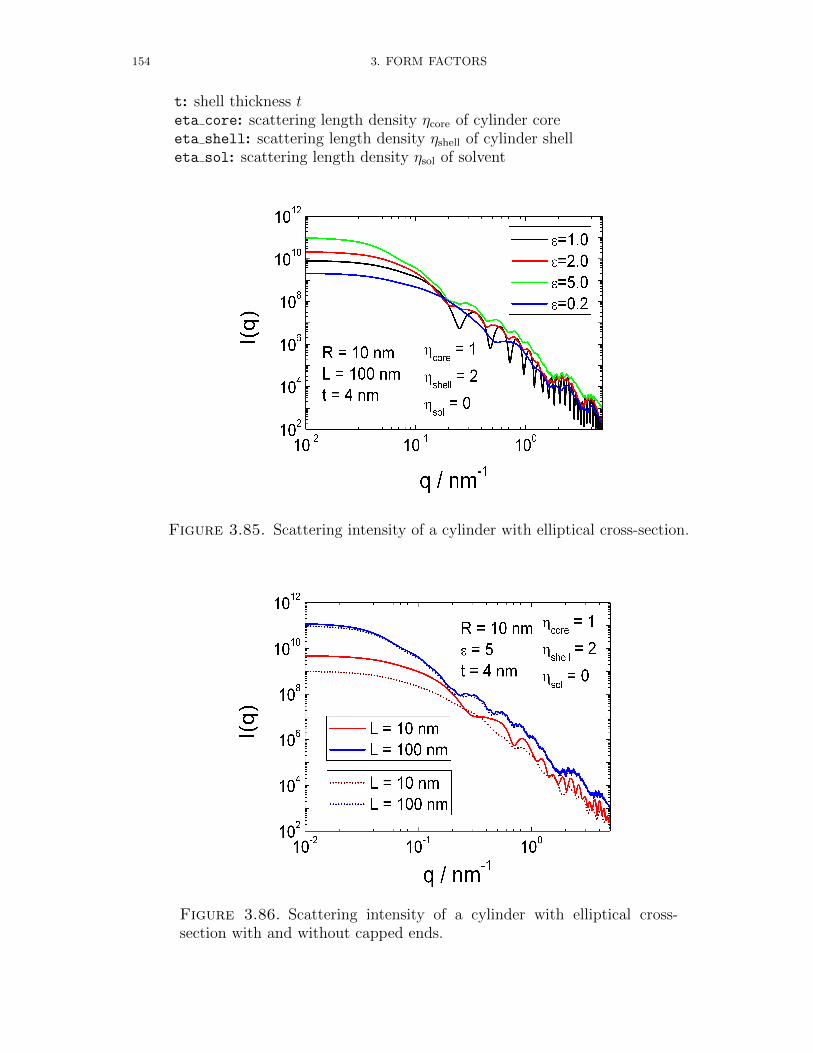
154 3. FORM FACTORS
t: shell thickness teta core: scattering length density ηcore of cylinder coreeta shell: scattering length density ηshell of cylinder shelleta sol: scattering length density ηsol of solvent
Figure 3.85. Scattering intensity of a cylinder with elliptical cross-section.
Figure 3.86. Scattering intensity of a cylinder with elliptical cross-section with and without capped ends.
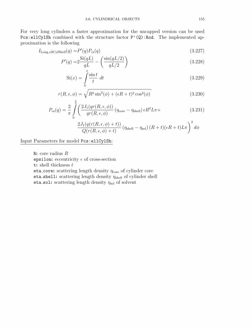
3.6. CYLINDRICAL OBJECTS 155
For very long cylinders a faster approximation for the uncapped version can be usedPcs:ellCylSh combined with the structure factor P’(Q):Rod. The implemented ap-proximation is the following
ILong ellCylShell(q) =P ′(q)Pcs(q) (3.227)
P ′(q) =2Si(qL)
qL−(
sin(qL/2)
qL/2
)(3.228)
Si(x) =
x∫0
sin t
tdt (3.229)
r(R, ε, φ) =√R2 sin2(φ) + (εR + t)2 cos2(φ) (3.230)
Pcs(q) =2
π
π2∫
0
(2J1(qr(R, ε, φ))
qr(R, ε, φ)(ηcore − ηshell) εR
2Lπ+ (3.231)
2J1(q(r(R, ε, φ) + t))
Q(r(R, ε, φ) + t)(ηshell − ηsol) (R + t)(εR + t)Lπ
)2
dφ
Input Parameters for model Pcs:ellCylSh:
R: core radius Repsilon: eccentricity ε of cross-sectiont: shell thickness teta core: scattering length density ηcore of cylinder coreeta shell: scattering length density ηshell of cylinder shelleta sol: scattering length density ηsol of solvent
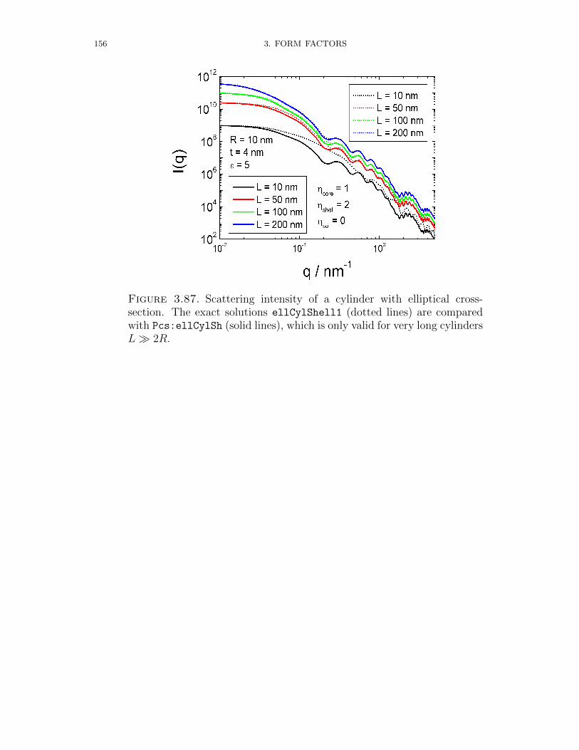
156 3. FORM FACTORS
Figure 3.87. Scattering intensity of a cylinder with elliptical cross-section. The exact solutions ellCylShell1 (dotted lines) are comparedwith Pcs:ellCylSh (solid lines), which is only valid for very long cylindersL 2R.
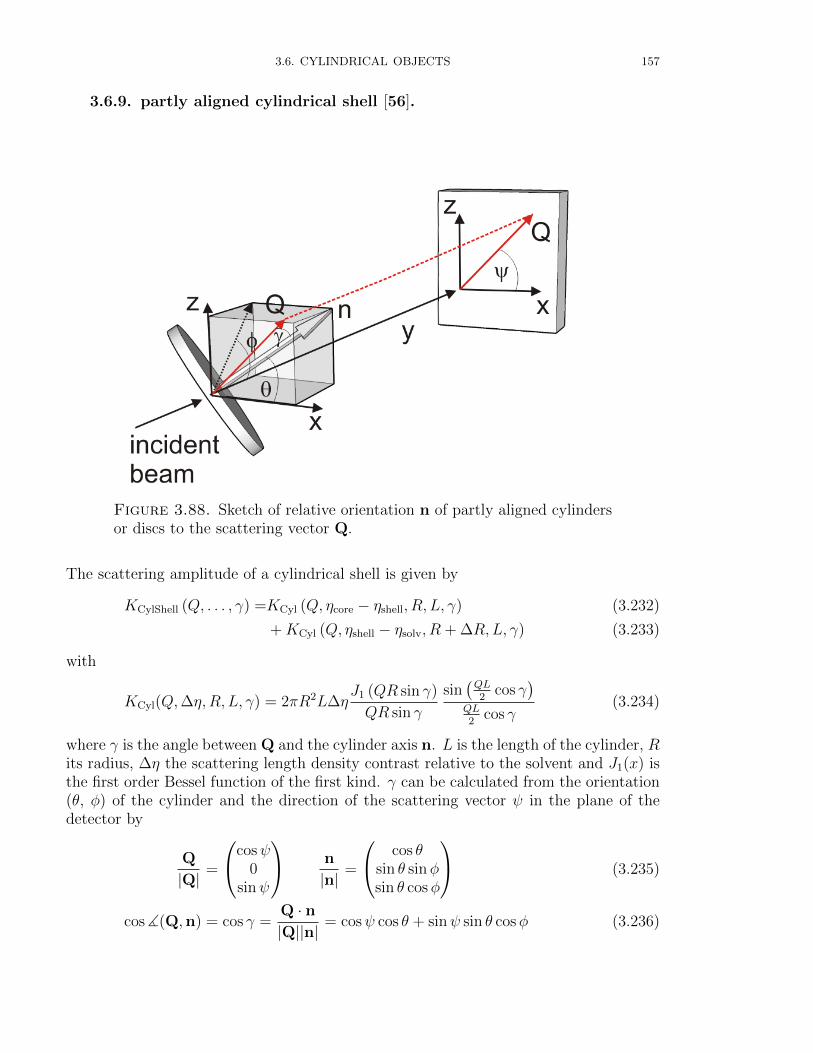
3.6. CYLINDRICAL OBJECTS 157
3.6.9. partly aligned cylindrical shell [56].
Figure 3.88. Sketch of relative orientation n of partly aligned cylindersor discs to the scattering vector Q.
The scattering amplitude of a cylindrical shell is given by
KCylShell (Q, . . . , γ) =KCyl (Q, ηcore − ηshell, R, L, γ) (3.232)
+KCyl (Q, ηshell − ηsolv, R + ∆R,L, γ) (3.233)
with
KCyl(Q,∆η,R, L, γ) = 2πR2L∆ηJ1 (QR sin γ)
QR sin γ
sin(QL2
cos γ)
QL2
cos γ(3.234)
where γ is the angle between Q and the cylinder axis n. L is the length of the cylinder, Rits radius, ∆η the scattering length density contrast relative to the solvent and J1(x) isthe first order Bessel function of the first kind. γ can be calculated from the orientation(θ, φ) of the cylinder and the direction of the scattering vector ψ in the plane of thedetector by
Q
|Q|=
cosψ0
sinψ
n
|n|=
cos θsin θ sinφsin θ cosφ
(3.235)
cos](Q,n) = cos γ =Q · n|Q||n|
= cosψ cos θ + sinψ sin θ cosφ (3.236)

158 3. FORM FACTORS
If the orientation distribution of the orientation vector n is described by p(θ, φ) so thatthe scattering intensity is given by
Ip.a.CylShell(Q) =
π∫0
dθ
2π∫0
dφ KCylShell (Q, . . . , γ) p(θ, φ) sin(θ) (3.237)
For this form factor it is assumed that the orientation distribution is independent of φ, i.e.p(θ, φ) = p(θ) and that p(θ) = p(π − θ), which means that turning the cylinder by 180
results in the same scattering intensity. Instead of assuming a special parametrizationof p(θ) the orientation distribution was expanded in terms of Legendre polynomialsPl(cos(θ))
p(θ) =∞∑
l=0,even
2l + 1
2〈Pl〉 Pl(cos(θ)) (3.238)
Due to the symmetrie p(θ) = p(π − θ) all terms with odd values for l are zero and onlythe even terms needs to be considered. For this form factor the first three terms up tol = 6 are implemented. As
∫ π0p(θ) sin θ dθ = 1 the zero order parameter is one 〈P0〉 = 1.
Input Parameters for model partly aligned CylShell:
R: core radius RDR: shell thickness ∆RL: cylinder length Leta core: scattering length density ηcore of cylinder coreeta shell: scattering length density ηshell of cylinder shelleta solv: scattering length density ηsolv of solventpsi: direction ψ of the scattering vector in the plane of the detectorP2: order parameter 〈P2〉P4: order parameter 〈P4〉P6: order parameter 〈P6〉
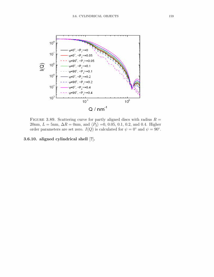
3.6. CYLINDRICAL OBJECTS 159
Figure 3.89. Scattering curve for partly aligned discs with radius R =20nm, L = 5nm, ∆R = 0nm, and 〈P2〉 =0, 0.05, 0.1, 0.2, and 0.4. Higherorder parameters are set zero. I(Q) is calculated for ψ = 0 and ψ = 90.
3.6.10. aligned cylindrical shell [?].
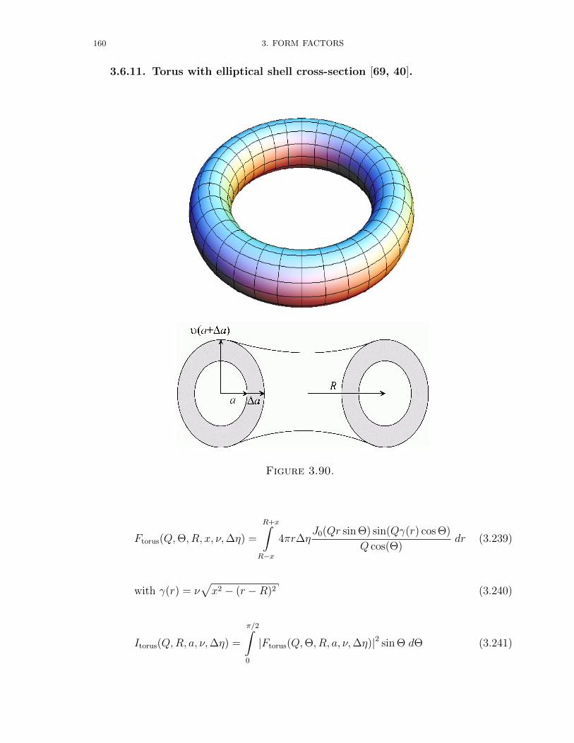
160 3. FORM FACTORS
3.6.11. Torus with elliptical shell cross-section [69, 40].
Figure 3.90.
Ftorus(Q,Θ, R, x, ν,∆η) =
R+x∫R−x
4πr∆ηJ0(Qr sin Θ) sin(Qγ(r) cos Θ)
Q cos(Θ)dr (3.239)
with γ(r) = ν√x2 − (r −R)2 (3.240)
Itorus(Q,R, a, ν,∆η) =
π/2∫0
|Ftorus(Q,Θ, R, a, ν,∆η)|2 sin Θ dΘ (3.241)
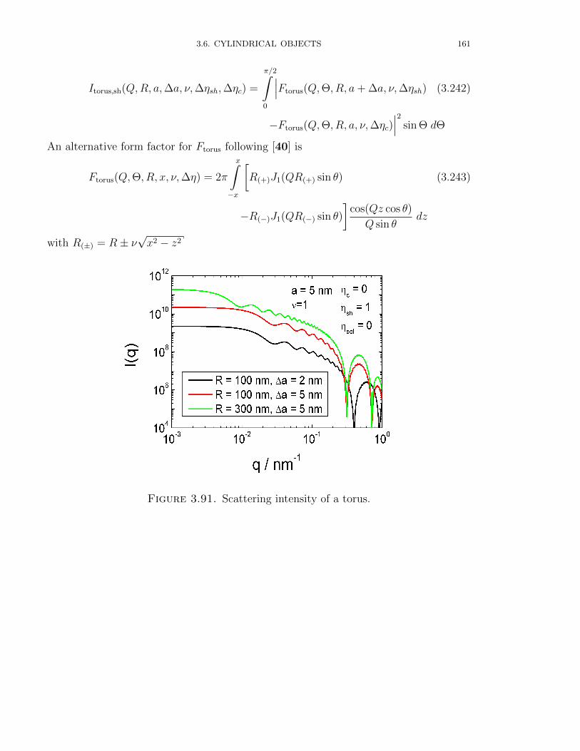
3.6. CYLINDRICAL OBJECTS 161
Itorus,sh(Q,R, a,∆a, ν,∆ηsh,∆ηc) =
π/2∫0
∣∣∣Ftorus(Q,Θ, R, a+ ∆a, ν,∆ηsh) (3.242)
−Ftorus(Q,Θ, R, a, ν,∆ηc)∣∣∣2 sin Θ dΘ
An alternative form factor for Ftorus following [40] is
Ftorus(Q,Θ, R, x, ν,∆η) = 2π
x∫−x
[R(+)J1(QR(+) sin θ) (3.243)
−R(−)J1(QR(−) sin θ)
]cos(Qz cos θ)
Q sin θdz
with R(±) = R± ν√x2 − z2
Figure 3.91. Scattering intensity of a torus.

162 3. FORM FACTORS
3.6.12. stacked tori with elliptical shell cross-section.
Figure 3.92.
Fstackedtori(Q,Θ, R, x, ν,∆η,∆D,N) = (3.244)
N∑n=1
R+x∫R−x
4πr∆ηJ0(Qr sin Θ) sin(Q(γ(r) + 2(n−1)−(N−1)
4∆D) cos Θ)
Q cos(Θ)dr
The scattering intensity is than calculated in the same way as for a single torus with anelliptical shell cross-section.
3.7. LOCAL PLANAR OBJECTS 163
3.7. Local Planar Objects
The form factor of very anisotropic particles with local planar geometry can beshown to factorize (see, e.g. [117]) into a cross-section form factor Pcs(Q) for the shorterdimensions and a shape factor P ′(Q) for the larger dimension:
Pplanar(Q) = P ′(Q)Pcs(Q) (3.245)
The factorization in the cross-section factor Pcs(Q), which only depends on param-eters describing the inner structure of the layer with short dimensions and the shapefactor P ′(Q), describing the overall shape in the larger dimension has the big advantagewhen both the shorter dimension as well as the larger dimensions have a polydispersity.In this case we do not end up with a double integral but rather a product of two inte-grals when both a short and a large dimension have a polydispersity. This speeds up thenumerical computation significantly. Therefore the following form factors already havea polydispersity parameter included.
3.7.1. Shape factors P ′(Q).The shape form factor P ′(Q) are normalized for Q → 0 on the squared surfacearea S (limQ→0 P
′(Q) = S2) and can be that of an infinitely thin disc, sphericalshell, elliptical shell, or cylindrical shell: The shape factors are accessible as a struc-ture factor under [anisotropic obj.|P’(Q):local planar geometry|P’(Q) xxx]
and using the monodisperse approximation. Actually these shape factors areforeseen to be used with the cross-section factors available as form factors under[anisotropic obj.|Pcs(Q) for planar obj.|Pcs(Q) xxx]. The shape factors arealso available in combination with some cross-section factors as form factors under[planar obj.].
3.7.1.1. Polydisperse infinitesimal thin discs.
P ′disc(Q,R) =2π2R4
(QR)2
(1− J1(2QR)
QR
)(3.246)
The polydispersity is included as a LogNormal-distribution from section 6.4 by
P ′ThinDiscs(Q,R, σ) =
∞∫0
LogNorm(R′, R, σ, 1)P ′disc(Q,R′) dR′ (3.247)
3.7.1.2. Infinitesimal thin spherical shell.
P ′sph. shell(Q,R) =
(4πR2 sinQR
QR
)2
(3.248)
(3.249)
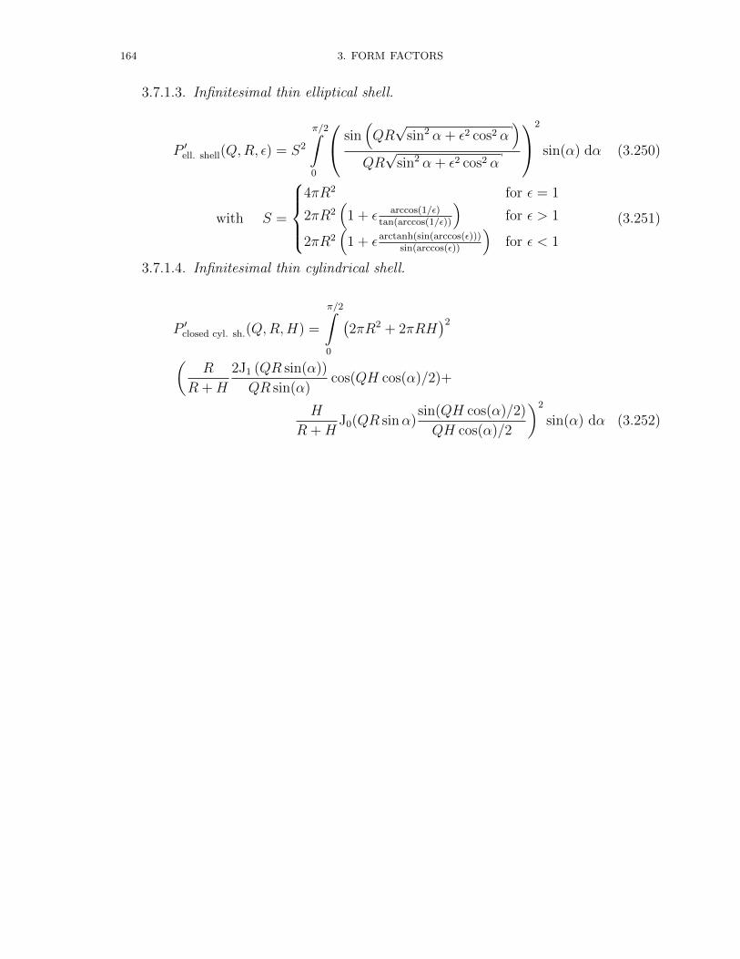
164 3. FORM FACTORS
3.7.1.3. Infinitesimal thin elliptical shell.
P ′ell. shell(Q,R, ε) = S2
π/2∫0
sin(QR√
sin2 α + ε2 cos2 α)
QR√
sin2 α + ε2 cos2 α
2
sin(α) dα (3.250)
with S =
4πR2 for ε = 1
2πR2(
1 + ε arccos(1/ε)tan(arccos(1/ε))
)for ε > 1
2πR2(
1 + εarctanh(sin(arccos(ε)))sin(arccos(ε))
)for ε < 1
(3.251)
3.7.1.4. Infinitesimal thin cylindrical shell.
P ′closed cyl. sh.(Q,R,H) =
π/2∫0
(2πR2 + 2πRH
)2
(R
R +H
2J1 (QR sin(α))
QR sin(α)cos(QH cos(α)/2)+
H
R +HJ0(QR sinα)
sin(QH cos(α)/2)
QH cos(α)/2
)2
sin(α) dα (3.252)
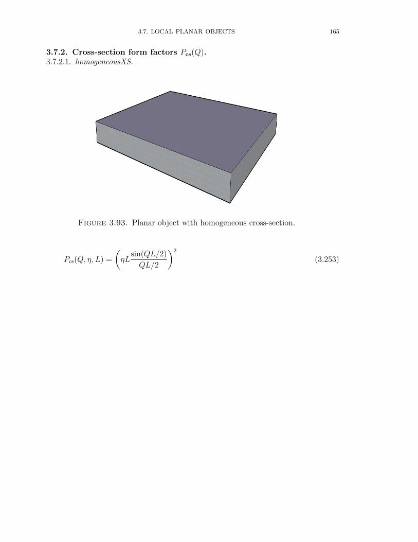
3.7. LOCAL PLANAR OBJECTS 165
3.7.2. Cross-section form factors Pcs(Q).3.7.2.1. homogeneousXS.
Figure 3.93. Planar object with homogeneous cross-section.
Pcs(Q, η, L) =
(ηL
sin(QL/2)
QL/2
)2
(3.253)
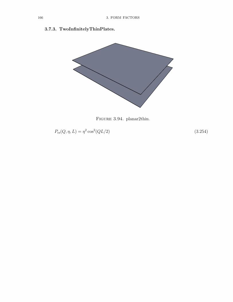
166 3. FORM FACTORS
3.7.3. TwoInfinitelyThinPlates.
Figure 3.94. planar2thin.
Pcs(Q, η, L) = η2 cos2(QL/2) (3.254)
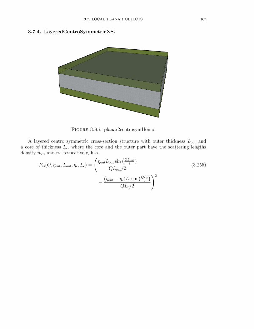
3.7. LOCAL PLANAR OBJECTS 167
3.7.4. LayeredCentroSymmetricXS.
Figure 3.95. planar2centrosymHomo.
A layered centro symmetric cross-section structure with outer thickness Lout anda core of thickness Lc, where the core and the outer part have the scattering lengthsdensity ηout and ηc, respectively, has
Pcs(Q, ηout, Lout, ηc, Lc) =
(ηoutLout sin
(QLout
2
)QLout/2
(3.255)
−(ηout − ηc)Lc sin
(QLc
2
)QLc/2
)2
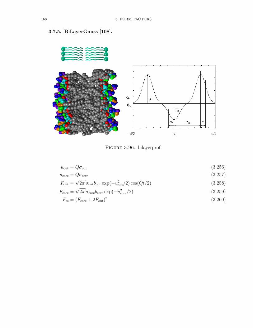
168 3. FORM FACTORS
3.7.5. BiLayerGauss [108].
Figure 3.96. bilayerprof.
uout = Qσout (3.256)
ucore = Qσcore (3.257)
Fout =√
2π σoutbout exp(−u2out/2) cos(Qt/2) (3.258)
Fcore =√
2π σcorebcore exp(−u2core/2) (3.259)
Pcs = (Fcore + 2Fout)2 (3.260)
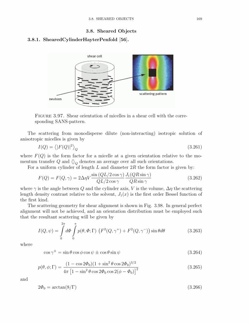
3.8. SHEARED OBJECTS 169
3.8. Sheared Objects
3.8.1. ShearedCylinderHayterPenfold [56].
Figure 3.97. Shear orientation of micelles in a shear cell with the corre-sponding SANS-pattern.
The scattering from monodisperse dilute (non-interacting) isotropic solution ofanisotropic micelles is given by
I(Q) =⟨|F (Q)|2
⟩Q
(3.261)
where F (Q) is the form factor for a micelle at a given orientation relative to the mo-mentum transfer Q and 〈〉Q denotes an average over all such orientations.
For a uniform cylinder of length L and diameter 2R the form factor is given by:
F (Q) = F (Q, γ) = 2∆ηVsin (QL/2 cos γ)
QL/2 cos γ
J1(QR sin γ)
QR sin γ(3.262)
where γ is the angle between Q and the cylinder axis, V is the volume, ∆η the scatteringlength density contrast relative to the solvent, J1(x) is the first order Bessel function ofthe first kind.
The scattering geometry for shear alignment is shown in Fig. 3.98. In general perfectalignment will not be achieved, and an orientation distribution must be employed suchthat the resultant scattering will be given by
I(Q,ψ) =
2π∫0
dΦ
π∫0
p(θ, Φ; Γ)(F 2(Q, γ+) + F 2(Q, γ−)
)sin θdθ (3.263)
where
cos γ± = sin θ cosφ cosψ ± cos θ sinψ (3.264)
p(θ, φ; Γ) =(1− cos 2Φ0)(1 + sin2 θ cos 2Φ0)3/2
4π[1− sin2 θ cos 2Φ0 cos 2(φ− Φ0)
]2 (3.265)
and
2Φ0 = arctan(8/Γ) (3.266)
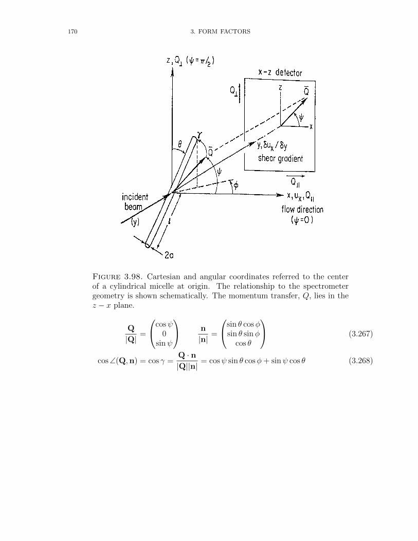
170 3. FORM FACTORS
Figure 3.98. Cartesian and angular coordinates referred to the centerof a cylindrical micelle at origin. The relationship to the spectrometergeometry is shown schematically. The momentum transfer, Q, lies in thez − x plane.
Q
|Q|=
cosψ0
sinψ
n
|n|=
sin θ cosφsin θ sinφ
cos θ
(3.267)
cos∠(Q,n) = cos γ =Q · n|Q||n|
= cosψ sin θ cosφ+ sinψ cos θ (3.268)
3.8. SHEARED OBJECTS 171
3.8.2. ShearedCylinderBoltzmann.
p(θ, φ; θ) = exp(−θ/θ) (3.269)
cos γ± = sin θ cosφ cosψ ± cos θ sinψ (3.270)
172 3. FORM FACTORS
3.8.3. ShearedCylinderGaussian.
p(θ, φ; θ) = exp(−(θ/θ)2) (3.271)
cos γ± = sin θ cosφ cosψ ± cos θ sinψ (3.272)
3.8. SHEARED OBJECTS 173
3.8.4. ShearedCylinderHeaviside.
p(θ, φ; θ) = Θ[θ − θ] (3.273)
cos γ± = sin θ cosφ cosψ ± cos θ sinψ (3.274)
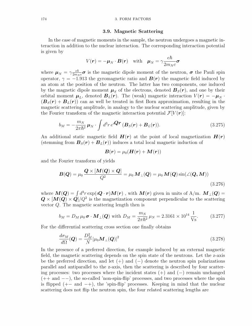
174 3. FORM FACTORS
3.9. Magnetic Scattering
In the case of magnetic moments in the sample, the neutron undergoes a magnetic in-teraction in addition to the nuclear interaction. The corresponding interaction potentialis given by
V (r) = −µN ·B(r) with µN = γe~
2mNcσ
where µN = γ e~2mN c
σ is the magnetic dipole moment of the neutron, σ the Pauli spin
operator, γ = −1.913 the gyromagnetic ratio and B(r) the magnetic field induced byan atom at the position of the neutron. The latter has two components, one inducedby the magnetic dipole moment µS of the electrons, denoted BS(r), and one by theirorbital moment µL, denoted BL(r). The (weak) magnetic interaction V (r) = −µN ·(BS(r) + BL(r)) can as well be treated in first Born approximation, resulting in themagnetic scattering amplitude, in analogy to the nuclear scattering amplitude, given bythe Fourier transform of the magnetic interaction potential F [V (r)]:
bM = − mN
2π~2µN ·
∫d3r eıQr (BS(r) +BL(r)). (3.275)
An additional static magnetic field H(r) at the point of local magnetization H(r)(stemming from BS(r) +BL(r)) induces a total local magnetic induction of
B(r) = µ0(H(r) +M(r))
and the Fourier transform of yields
B(Q) = µ0Q× [M(Q)×Q]
Q2= µ0M⊥(Q) = µ0M (Q) sin(∠(Q,M))
(3.276)
where M(Q) =∫d3r exp(ıQ · r)M(r) , with M (r) given in units of A/m. M⊥(Q) =
Q × [M(Q) ×Q]/Q2 is the magnetization component perpendicular to the scatteringvector Q. The magnetic scattering length then is
bM = DM µ0 σ ·M⊥(Q) with DM =mN
2π~2µN = 2.3161× 10¹⁴ 1
Vs. (3.277)
For the differential scattering cross section one finally obtains
dσMdΩ
(Q) =D2M
N|µ0M⊥(Q)|2 (3.278)
In the presence of a preferred direction, for example induced by an external magneticfield, the magnetic scattering depends on the spin state of the neutrons. Let the z-axisbe the preferred direction, and let (+) and (−) denote the neutron spin polarizationsparallel and antiparallel to the z-axis, then the scattering is described by four scatter-ing processes: two processes where the incident states (+) and (−) remain unchanged(++ and −−), the so-called ’non-spin-flip’ processes, and two processes where the spinis flipped (+− and −+), the ’spin-flip’ processes. Keeping in mind that the nuclearscattering does not flip the neutron spin, the four related scattering lengths are
3.9. MAGNETIC SCATTERING 175
b±± = bN ∓DM µ0M⊥x (3.279)
b±∓ = −DM µ0 (M⊥z ± ıM⊥y). (3.280)
Hereby bN is the nuclear scattering length. For an unpolarized neutron beam (whichmay be taken as composed of 50% (+) and 50% (−) polarization) the square of themodulus of the scattering length is
(b2++ + b2
−− + b2+− + b2
−+)/2 = b2N +D2
Mµ20M
2⊥. (3.281)
The differential cross section of the unpolarized neutron beam can therefore be describedby the sum of the nuclear and the magnetic cross section, without any cross terms.
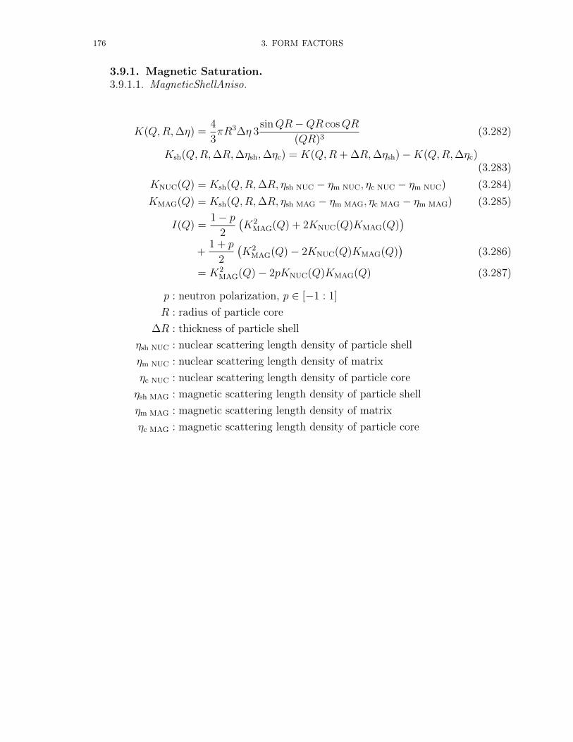
176 3. FORM FACTORS
3.9.1. Magnetic Saturation.3.9.1.1. MagneticShellAniso.
K(Q,R,∆η) =4
3πR3∆η 3
sinQR−QR cosQR
(QR)3(3.282)
Ksh(Q,R,∆R,∆ηsh,∆ηc) = K(Q,R + ∆R,∆ηsh)−K(Q,R,∆ηc)(3.283)
KNUC(Q) = Ksh(Q,R,∆R, ηsh NUC − ηm NUC, ηc NUC − ηm NUC) (3.284)
KMAG(Q) = Ksh(Q,R,∆R, ηsh MAG − ηm MAG, ηc MAG − ηm MAG) (3.285)
I(Q) =1− p
2
(K2
MAG(Q) + 2KNUC(Q)KMAG(Q))
+1 + p
2
(K2
MAG(Q)− 2KNUC(Q)KMAG(Q))
(3.286)
= K2MAG(Q)− 2pKNUC(Q)KMAG(Q) (3.287)
p : neutron polarization, p ∈ [−1 : 1]
R : radius of particle core
∆R : thickness of particle shell
ηsh NUC : nuclear scattering length density of particle shell
ηm NUC : nuclear scattering length density of matrix
ηc NUC : nuclear scattering length density of particle core
ηsh MAG : magnetic scattering length density of particle shell
ηm MAG : magnetic scattering length density of matrix
ηc MAG : magnetic scattering length density of particle core
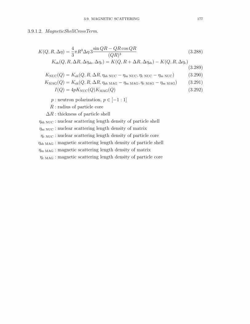
3.9. MAGNETIC SCATTERING 177
3.9.1.2. MagneticShellCrossTerm.
K(Q,R,∆η) =4
3πR3∆η 3
sinQR−QR cosQR
(QR)3(3.288)
Ksh(Q,R,∆R,∆ηsh,∆ηc) = K(Q,R + ∆R,∆ηsh)−K(Q,R,∆ηc)(3.289)
KNUC(Q) = Ksh(Q,R,∆R, ηsh NUC − ηm NUC, ηc NUC − ηm NUC) (3.290)
KMAG(Q) = Ksh(Q,R,∆R, ηsh MAG − ηm MAG, ηc MAG − ηm MAG) (3.291)
I(Q) = 4pKNUC(Q)KMAG(Q) (3.292)
p : neutron polarization, p ∈ [−1 : 1]
R : radius of particle core
∆R : thickness of particle shell
ηsh NUC : nuclear scattering length density of particle shell
ηm NUC : nuclear scattering length density of matrix
ηc NUC : nuclear scattering length density of particle core
ηsh MAG : magnetic scattering length density of particle shell
ηm MAG : magnetic scattering length density of matrix
ηc MAG : magnetic scattering length density of particle core

178 3. FORM FACTORS
3.9.1.3. MagneticShellPsi.
K(Q,R,∆η) =4
3πR3∆η 3
sinQR−QR cosQR
(QR)3(3.293)
Ksh(Q,R,∆R,∆ηsh,∆ηc) = K(Q,R + ∆R,∆ηsh)−K(Q,R,∆ηc)(3.294)
KNUC(Q) = Ksh(Q,R,∆R, ηsh NUC − ηm NUC, ηc NUC − ηm NUC) (3.295)
KMAG(Q) = Ksh(Q,R,∆R, ηsh MAG − ηm MAG, ηc MAG − ηm MAG) (3.296)
I(Q) = K2NUC(Q) +
(K2
MAG(Q)− 2pKNUC(Q)KMAG(Q))
sin2 Ψ (3.297)
p : neutron polarization, p ∈ [−1 : 1]
R : radius of particle core
Ψ : angle between Q and H
∆R : thickness of particle shell
ηsh NUC : nuclear scattering length density of particle shell
ηm NUC : nuclear scattering length density of matrix
ηc NUC : nuclear scattering length density of particle core
ηsh MAG : magnetic scattering length density of particle shell
ηm MAG : magnetic scattering length density of matrix
ηc MAG : magnetic scattering length density of particle core
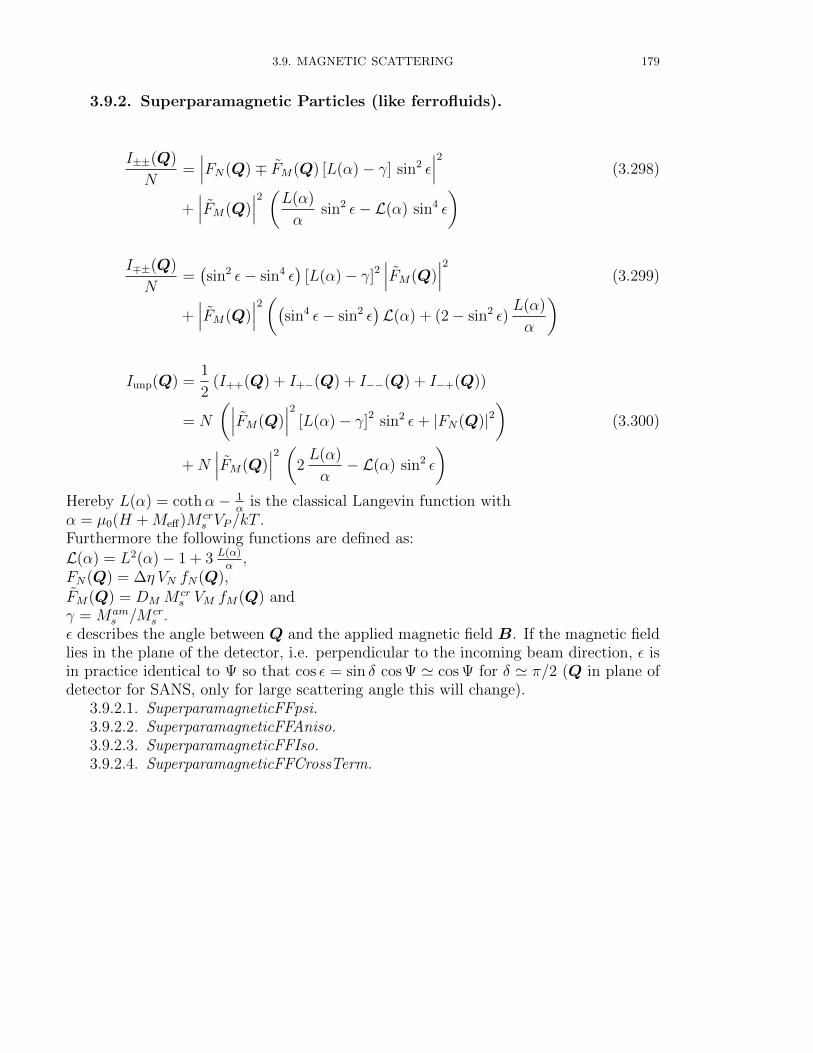
3.9. MAGNETIC SCATTERING 179
3.9.2. Superparamagnetic Particles (like ferrofluids).
I±±(Q)
N=∣∣∣FN(Q)∓ FM(Q) [L(α)− γ] sin2 ε
∣∣∣2 (3.298)
+∣∣∣FM(Q)
∣∣∣2 (L(α)
αsin2 ε− L(α) sin4 ε
)
I∓±(Q)
N=(sin2 ε− sin4 ε
)[L(α)− γ]2
∣∣∣FM(Q)∣∣∣2 (3.299)
+∣∣∣FM(Q)
∣∣∣2((sin4 ε− sin2 ε)L(α) + (2− sin2 ε)
L(α)
α
)
Iunp(Q) =1
2(I++(Q) + I+−(Q) + I−−(Q) + I−+(Q))
= N
(∣∣∣FM(Q)∣∣∣2 [L(α)− γ]2 sin2 ε+ |FN(Q)|2
)(3.300)
+N∣∣∣FM(Q)
∣∣∣2 (2L(α)
α− L(α) sin2 ε
)Hereby L(α) = cothα− 1
αis the classical Langevin function with
α = µ0(H +Meff)M crs VP/kT .
Furthermore the following functions are defined as:
L(α) = L2(α)− 1 + 3 L(α)α
,FN(Q) = ∆η VN fN(Q),FM(Q) = DM M cr
s VM fM(Q) andγ = Mam
s /M crs .
ε describes the angle between Q and the applied magnetic field B. If the magnetic fieldlies in the plane of the detector, i.e. perpendicular to the incoming beam direction, ε isin practice identical to Ψ so that cos ε = sin δ cos Ψ ' cos Ψ for δ ' π/2 (Q in plane ofdetector for SANS, only for large scattering angle this will change).
3.9.2.1. SuperparamagneticFFpsi.3.9.2.2. SuperparamagneticFFAniso.3.9.2.3. SuperparamagneticFFIso.3.9.2.4. SuperparamagneticFFCrossTerm.
180 3. FORM FACTORS
3.10. Lorenz-Mie Form Factors for Static Light Scattering
Mie theory, also called Lorenz-Mie theory [96, 139, 14], is a complete mathematical-physical theory of the scattering of electromagnetic radiation by spherical particles. Mietheory is named after its developer German physicist Gustav Mie (1868 Rostock - 1957Freiburg im Breisgau) and Danish physicist Ludvig Lorenz (1829-1891) who indepen-dently developed the theory of electromagnetic plane wave scattering by a dielectricsphere in 1908.
Mie scattering describes the scattering of electromagnetic radiation by spherical par-ticles of any size r, relative to the wavelength, λ. Since the cases r λ and r λ arecovered by Rayleigh (dipole) scattering and geometric scattering theories, respectively,Mie scattering often refers to the case of r ∼ λ.
3.10.1. MieSphere.
The Mie scattering formulae are given in several books (Van de Hulst, 1957; Kerker,1969; Deirmendjian, 1969) and by Dave (1968a, 1969a), although not always in the formsmost suited to computation. The algorithm used here is based on the MIEV0 packagedescribed in [153, 154]. The following input values are used:
Θ = 2 arcsin(Qλ/(4π)) with Q < Qmax = 4π/λ
R = radius of scattering sphere
λ = wavelength of incident plane wave inside the solvent
m = complex refractive index of sphere relative to surrounding medium
= mre − imim
|m| ≥ 1 and mim ≥ 0
or
|m| < 1 and mim = 0
pol = 0 unpolarized light
pol = 1 parallel to scattering plane polarized light
pol = −1 perpendicular to scattering plane polarized light
|m| < 1 would, for example, include visible light scattering from air bubbles in water.
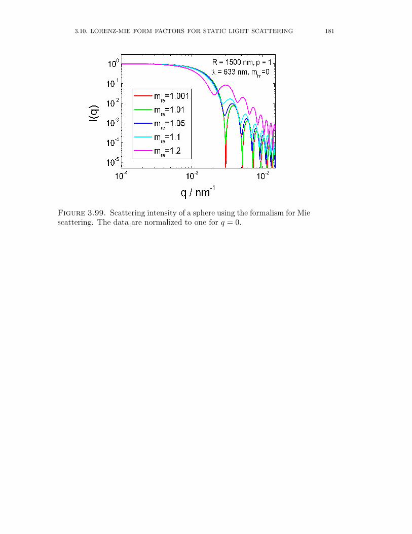
3.10. LORENZ-MIE FORM FACTORS FOR STATIC LIGHT SCATTERING 181
Figure 3.99. Scattering intensity of a sphere using the formalism for Miescattering. The data are normalized to one for q = 0.
182 3. FORM FACTORS
3.10.2. MieShell.
This form factor is basing on the version of MieLay, which computes electromag-netic scattering by a stratified sphere, i.e. a particle consisting of a spherical coresurrounded by a spherical shell. The surrounding medium is assumed to have refractiveindex unity. The formulas, manipulated to avoid the ill-conditioning that plagued ear-lier formulations, were published in [136]. Further documentation, including definitonsof input and output arguments, is inside the single precision version of this program(SUBROUTINE MieLay, available by anonymous ftp from climate.gsfc.nasa.gov in di-rectory pub/wiscombe). The following input values are used:
Θ = 2 arcsin(Qλ/(4π)) with Q < Qmax = 4π/λ
Rc = radius of the core of scattering sphere
Rsh = thickness of the shell of scattering sphere
λ = wavelength of incident plane wave inside the solvent
mc = complex refractive index of core relative to surrounding medium
= mc,re − imc,im
|mc| ≥ 1 and mc,im ≥ 0
or
|mc| < 1 and mc,im = 0
ms = complex refractive index of core relative to surrounding medium
= ms,re − ims,im
pol = 0 unpolarized light
pol = 1 parallel to scattering plane polarized light
pol = −1 perpendicular to scattering plane polarized light
|m| < 1 would, for example, include visible light scattering from air bubbles in water.
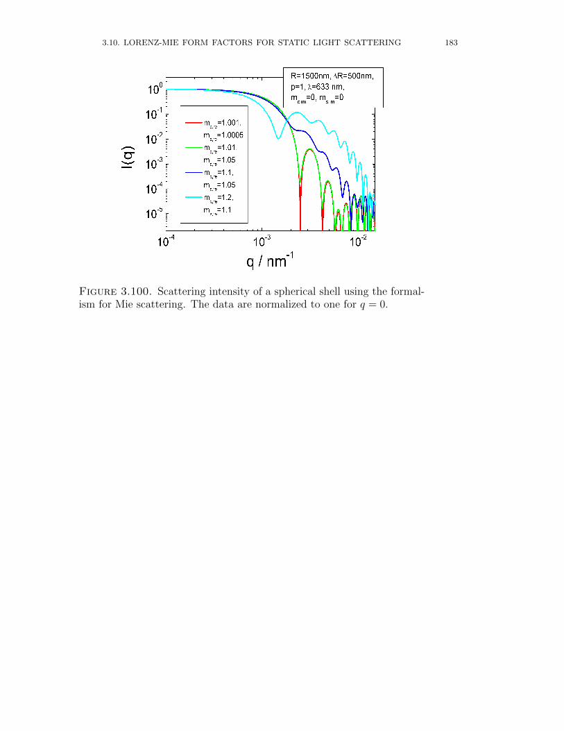
3.10. LORENZ-MIE FORM FACTORS FOR STATIC LIGHT SCATTERING 183
Figure 3.100. Scattering intensity of a spherical shell using the formal-ism for Mie scattering. The data are normalized to one for q = 0.

184 3. FORM FACTORS
3.11. Other functions3.11.1. DLS Sphere RDG.
This function has been implemented to simulate the relaxation signal g2(t)−1 = g21(t)
of a DLS (dynamic light scattering) measurement. The Q dependent contribution to therelaxation signal by particles of different radius R is considered by weighting g2(t) − 1with the form factor of sperical particles in Raylay-Debye-Gans approximation:
IDLS Sphere RDG(t, η, T,Q) =
∞∫0
N(R) K2sp(Q,R) e−DQ
2t dR (3.301)
with
D =kBT
6πηR
Ksp(Q,R) =4
3πR3 3
sinQR−QR cosQR
(QR)3
R : radius
T : temperature
η : viscosity
Q : scattering vector
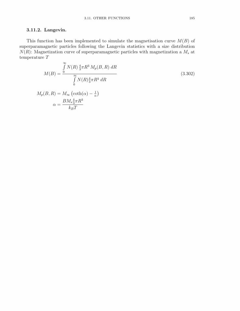
3.11. OTHER FUNCTIONS 185
3.11.2. Langevin.
This function has been implemented to simulate the magnetisation curve M(B) ofsuperparamagnetic particles following the Langevin statistics with a size distributionN(R): Magnetization curve of superparamagnetic particles with magnetization a Ms attemperature T
M(B) =
∞∫0
N(R) 43πR3Mp(B,R) dR
∞∫0
N(R)43πR3 dR
(3.302)
Mp(B,R) = M∞(coth(α)− 1
α
)α =
BMs43πR3
kBT
186 3. FORM FACTORS
3.11.3. SuperParStroboPsi.
In the following the scattering of polarized incident neutrons with polarization anal-ysis (POLARIS) is described. Experimental measured scattering signal are always amixture of the spin dependent scattering cross-sections I±±(Q) and I±∓(Q). The rel-ative contribution of these cross-sections to the measured cross-section depend on thepolarisation of the polarizer Ppol the efficiency of the spin flipper ε and the transmissionvalues T± of the polarization analyzer, which is assumed to be an opaque He-filter. Ifthe neutron polarization of the polarizer is Ppol ∈ [−1; 1] and the spin flipper is off theincident polarisation on the sample Pin is given by
Pin = Ppol =N+ −N−N+ +N−
= n+ − n− (3.303a)
with
n+ =N+
N+ +N−and n− =
N−N+ +N−
(3.303b)
⇒ n+ =1 + Ppol
2and n− =
1− Ppol2
(3.303c)
N± are the number of incident neutrons with spin polarizations up (+) and down (−).After switching on the spin flipper, which works with an efficiency of ε ∈ [0; 1] (ε = 0:flipper off, ε / 1 : flipper on), one gets
n+(Ppol, ε) = ε1− Ppol
2+ (1− ε) 1 + Ppol
2
=1− εPpol
2and
n−(Ppol, ε) = ε1 + Ppol
2+ (1− ε) 1− Ppol
2
=1 + εPpol
2
The efficiency of the analyzer to filter spin up (+) or spin down (−) neutrons is given incase of an opaque spin filter by its transmission T±(t) ∈ [0; 1], which can be a functionof time, so that the measured scattering cross section Im(Q) is given by
Im(Q) = n+(Ppol, ε)T+(t)I++(Q) + n+(Ppol, ε)T−(t)I+−(Q)
+ n−(Ppol, ε)T−(t)I−−(Q) + n−(Ppol, ε)T+(t)I−+(Q)(3.304)
The spin dependent scattering intensities of magnetic particles with an orientation dis-tribution f (θ, φ) of its magnetic moment can easily be calculated in terms of orderparameters Sl if one assumes that the particle are spherical symmetric or the orienta-tion of the magnetic moment of a particle is not correlated to the particle orientation.Furthermore it will be assumed that an external magnetic field is applied perpendicularto the incident neutron beam and that all orientations φ for a given angle θ, which isdefined as the angle between the magnetisation vector of the particle and the directionof the external field B have the same probability, i.e. the orientation distribution onlydepends on θ so that f (θ, φ) = f (θ). The orientation probability distribution function
3.11. OTHER FUNCTIONS 187
can be expanded in terms of a complete set of orthogonal functions. Expanding it interms of Legendre polynomials Pl(cos θ) gives
f(θ) =∑l
clPl(cos θ) =∑l
2l + 1
2SlPl(cos θ) (3.305)
The expansion coefficients can be calculated by
cl =2l + 1
2
π∫0
f(θ)Pl(cos θ) sin θ dθ
or
Sl =
π∫0
f(θ)Pl(cos θ) sin θ dθ
(3.306)
The first three Legendre polynomials are defined by
P0(cos θ) = 1 (3.307a)
P1(cos θ) = cos θ (3.307b)
P2(cos θ) =1
2
(3 cos2 θ − 1
)(3.307c)
For superparamagnetic particle the orientation probability distribution is given by
f(θ) =α
4π sinhαexp(α cos θ) (3.308)
with α = BMpVp/(kBT ) being the Langevin parameter. For this orientation probabilitydistribution the first order parameters can be calculates as
S0 = 1 (3.309a)
S1 = L(α) = cothα− 1
α(3.309b)
S2 = 1− 3L(α)
α(3.309c)
The scattering from a system of many particles is obtained by summing up the scatteringamplitudes of all precipitates weighted by the phase shift at each particle position. Inthe decoupling approach scattering intensity is given by
dσ±±±∓
dΩ(Q) = N
⟨∣∣∣F±±±∓
(Q)∣∣∣2⟩+
∣∣∣⟨F±±±∓
(Q)⟩∣∣∣2(S(Q)− 1)
(3.310)
which consists of two terms. The first one depends only on the particle structure andcorresponds to the independent scattering of N particles, while the second one is also afunction of their statistical distribution and reflects the interparticle interference, whichis described by S(Q). The 〈〉 indicates an average over all possible configurations, sizesand orientations of the magnetic moments of the particles. The spin dependent scattering
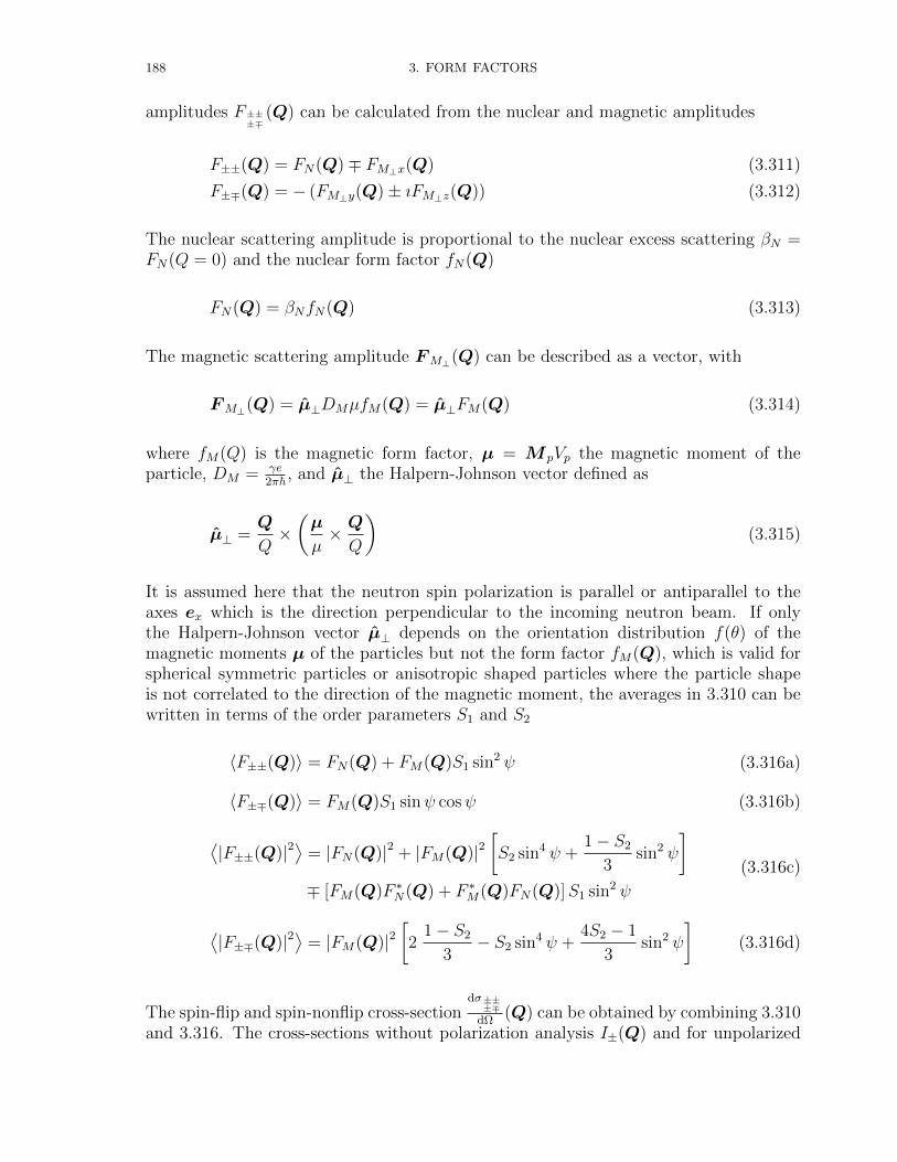
188 3. FORM FACTORS
amplitudes F±±±∓
(Q) can be calculated from the nuclear and magnetic amplitudes
F±±(Q) = FN(Q)∓ FM⊥x(Q) (3.311)
F±∓(Q) = − (FM⊥y(Q)± ıFM⊥z(Q)) (3.312)
The nuclear scattering amplitude is proportional to the nuclear excess scattering βN =FN(Q = 0) and the nuclear form factor fN(Q)
FN(Q) = βNfN(Q) (3.313)
The magnetic scattering amplitude FM⊥(Q) can be described as a vector, with
FM⊥(Q) = µ⊥DMµfM(Q) = µ⊥FM(Q) (3.314)
where fM(Q) is the magnetic form factor, µ = M pVp the magnetic moment of theparticle, DM = γe
2π~ , and µ⊥ the Halpern-Johnson vector defined as
µ⊥ =Q
Q×(µ
µ× QQ
)(3.315)
It is assumed here that the neutron spin polarization is parallel or antiparallel to theaxes ex which is the direction perpendicular to the incoming neutron beam. If onlythe Halpern-Johnson vector µ⊥ depends on the orientation distribution f(θ) of themagnetic moments µ of the particles but not the form factor fM(Q), which is valid forspherical symmetric particles or anisotropic shaped particles where the particle shapeis not correlated to the direction of the magnetic moment, the averages in 3.310 can bewritten in terms of the order parameters S1 and S2
〈F±±(Q)〉 = FN(Q) + FM(Q)S1 sin2 ψ (3.316a)
〈F±∓(Q)〉 = FM(Q)S1 sinψ cosψ (3.316b)
⟨|F±±(Q)|2
⟩= |FN(Q)|2 + |FM(Q)|2
[S2 sin4 ψ +
1− S2
3sin2 ψ
]∓ [FM(Q)F ∗N(Q) + F ∗M(Q)FN(Q)]S1 sin2 ψ
(3.316c)
⟨|F±∓(Q)|2
⟩= |FM(Q)|2
[2
1− S2
3− S2 sin4 ψ +
4S2 − 1
3sin2 ψ
](3.316d)
The spin-flip and spin-nonflip cross-sectiondσ±±±∓
dΩ(Q) can be obtained by combining 3.310
and 3.316. The cross-sections without polarization analysis I±(Q) and for unpolarized
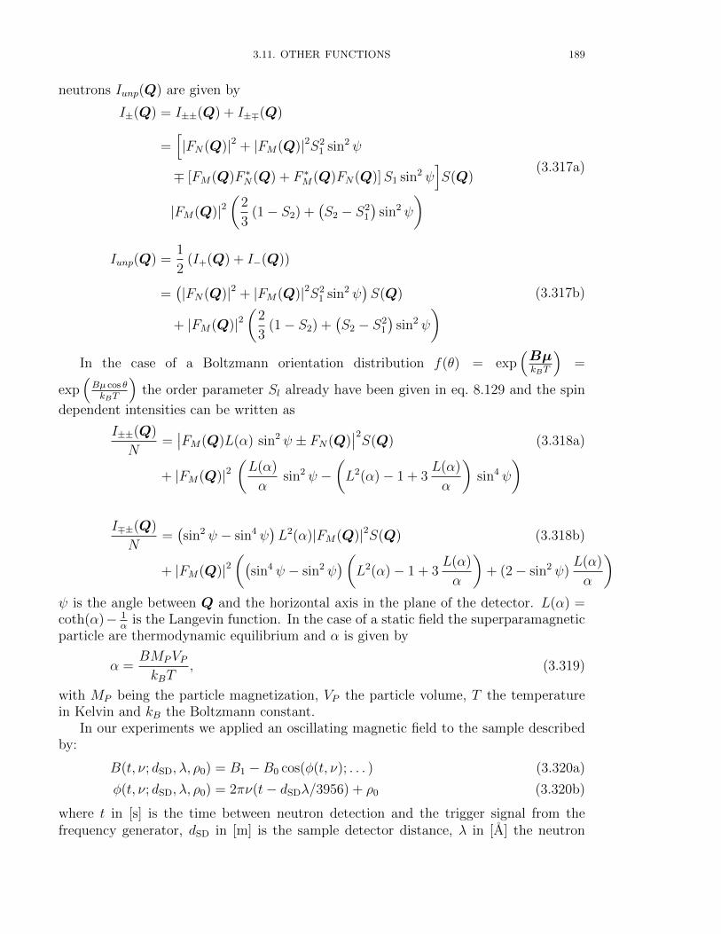
3.11. OTHER FUNCTIONS 189
neutrons Iunp(Q) are given by
I±(Q) = I±±(Q) + I±∓(Q)
=[|FN(Q)|2 + |FM(Q)|2S2
1 sin2 ψ
∓ [FM(Q)F ∗N(Q) + F ∗M(Q)FN(Q)]S1 sin2 ψ]S(Q)
|FM(Q)|2(
2
3(1− S2) +
(S2 − S2
1
)sin2 ψ
) (3.317a)
Iunp(Q) =1
2(I+(Q) + I−(Q))
=(|FN(Q)|2 + |FM(Q)|2S2
1 sin2 ψ)S(Q)
+ |FM(Q)|2(
2
3(1− S2) +
(S2 − S2
1
)sin2 ψ
) (3.317b)
In the case of a Boltzmann orientation distribution f(θ) = exp(BµkBT
)=
exp(Bµ cos θkBT
)the order parameter Sl already have been given in eq. 8.129 and the spin
dependent intensities can be written as
I±±(Q)
N=∣∣FM(Q)L(α) sin2 ψ ± FN(Q)
∣∣2S(Q) (3.318a)
+ |FM(Q)|2(L(α)
αsin2 ψ −
(L2(α)− 1 + 3
L(α)
α
)sin4 ψ
)
I∓±(Q)
N=(sin2 ψ − sin4 ψ
)L2(α)|FM(Q)|2S(Q) (3.318b)
+ |FM(Q)|2((
sin4 ψ − sin2 ψ)(
L2(α)− 1 + 3L(α)
α
)+ (2− sin2 ψ)
L(α)
α
)ψ is the angle between Q and the horizontal axis in the plane of the detector. L(α) =coth(α)− 1
αis the Langevin function. In the case of a static field the superparamagnetic
particle are thermodynamic equilibrium and α is given by
α =BMPVPkBT
, (3.319)
with MP being the particle magnetization, VP the particle volume, T the temperaturein Kelvin and kB the Boltzmann constant.
In our experiments we applied an oscillating magnetic field to the sample describedby:
B(t, ν; dSD, λ, ρ0) = B1 −B0 cos(φ(t, ν); . . . ) (3.320a)
φ(t, ν; dSD, λ, ρ0) = 2πν(t− dSDλ/3956) + ρ0 (3.320b)
where t in [s] is the time between neutron detection and the trigger signal from thefrequency generator, dSD in [m] is the sample detector distance, λ in [A] the neutron
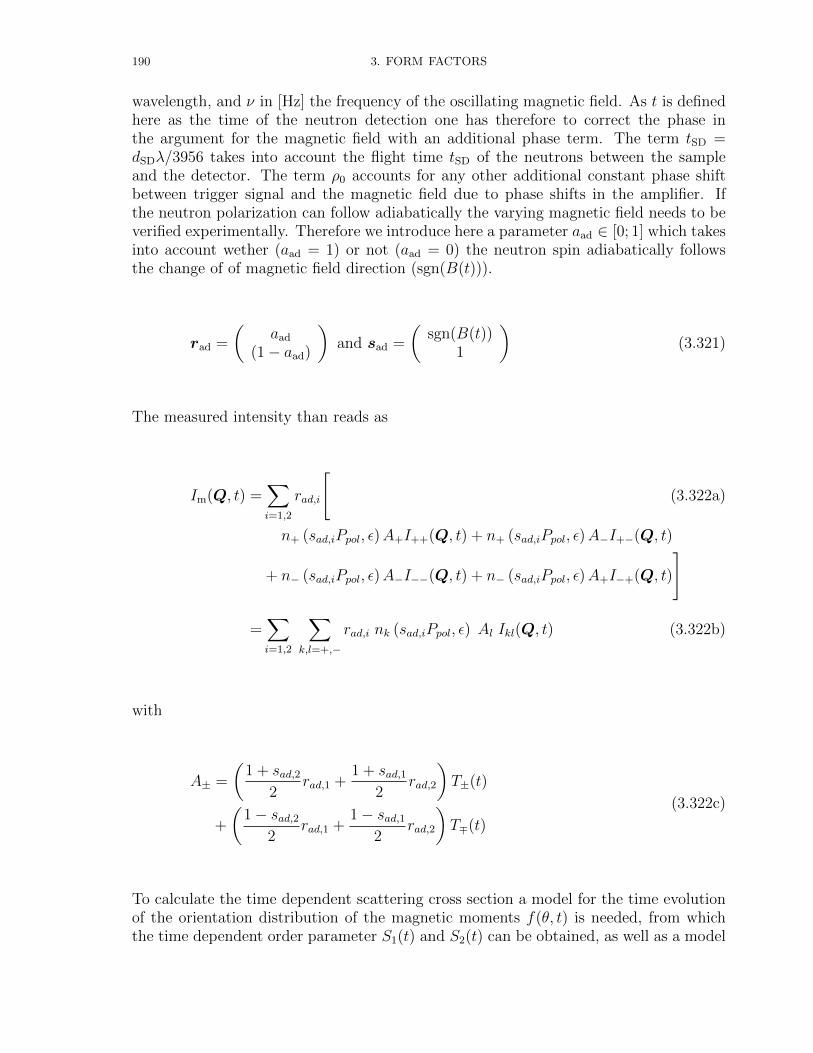
190 3. FORM FACTORS
wavelength, and ν in [Hz] the frequency of the oscillating magnetic field. As t is definedhere as the time of the neutron detection one has therefore to correct the phase inthe argument for the magnetic field with an additional phase term. The term tSD =dSDλ/3956 takes into account the flight time tSD of the neutrons between the sampleand the detector. The term ρ0 accounts for any other additional constant phase shiftbetween trigger signal and the magnetic field due to phase shifts in the amplifier. Ifthe neutron polarization can follow adiabatically the varying magnetic field needs to beverified experimentally. Therefore we introduce here a parameter aad ∈ [0; 1] which takesinto account wether (aad = 1) or not (aad = 0) the neutron spin adiabatically followsthe change of of magnetic field direction (sgn(B(t))).
rad =
(aad
(1− aad)
)and sad =
(sgn(B(t))
1
)(3.321)
The measured intensity than reads as
Im(Q, t) =∑i=1,2
rad,i
[(3.322a)
n+ (sad,iPpol, ε)A+I++(Q, t) + n+ (sad,iPpol, ε)A−I+−(Q, t)
+ n− (sad,iPpol, ε)A−I−−(Q, t) + n− (sad,iPpol, ε)A+I−+(Q, t)
]
=∑i=1,2
∑k,l=+,−
rad,i nk (sad,iPpol, ε) Al Ikl(Q, t) (3.322b)
with
A± =
(1 + sad,2
2rad,1 +
1 + sad,12
rad,2
)T±(t)
+
(1− sad,2
2rad,1 +
1− sad,12
rad,2
)T∓(t)
(3.322c)
To calculate the time dependent scattering cross section a model for the time evolutionof the orientation distribution of the magnetic moments f(θ, t) is needed, from whichthe time dependent order parameter S1(t) and S2(t) can be obtained, as well as a model
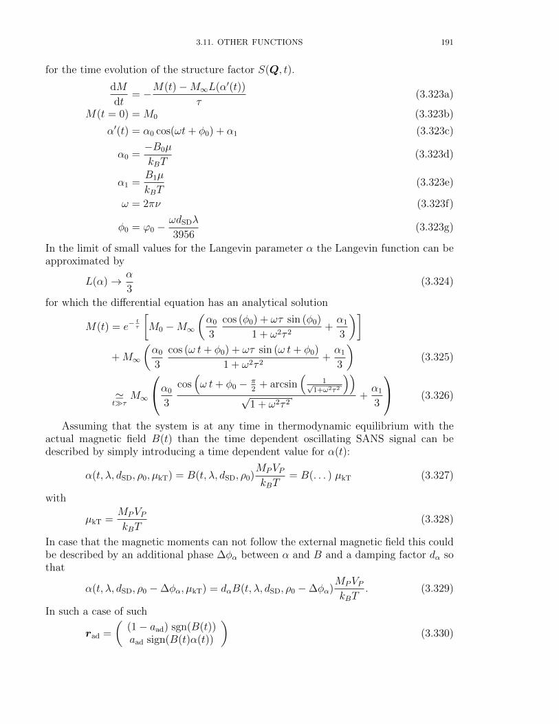
3.11. OTHER FUNCTIONS 191
for the time evolution of the structure factor S(Q, t).
dM
dt= −M(t)−M∞L(α′(t))
τ(3.323a)
M(t = 0) = M0 (3.323b)
α′(t) = α0 cos(ωt+ φ0) + α1 (3.323c)
α0 =−B0µ
kBT(3.323d)
α1 =B1µ
kBT(3.323e)
ω = 2πν (3.323f)
φ0 = ϕ0 −ωdSDλ
3956(3.323g)
In the limit of small values for the Langevin parameter α the Langevin function can beapproximated by
L(α)→ α
3(3.324)
for which the differential equation has an analytical solution
M(t) = e−tτ
[M0 −M∞
(α0
3
cos (φ0) + ωτ sin (φ0)
1 + ω2τ 2+α1
3
)]+M∞
(α0
3
cos (ω t+ φ0) + ωτ sin (ω t+ φ0)
1 + ω2τ 2+α1
3
)(3.325)
'tτ
M∞
α0
3
cos(ω t+ φ0 − π
2+ arcsin
(1√
1+ω2τ2
))√
1 + ω2τ 2+α1
3
(3.326)
Assuming that the system is at any time in thermodynamic equilibrium with theactual magnetic field B(t) than the time dependent oscillating SANS signal can bedescribed by simply introducing a time dependent value for α(t):
α(t, λ, dSD, ρ0, µkT) = B(t, λ, dSD, ρ0)MPVPkBT
= B(. . . ) µkT (3.327)
with
µkT =MPVPkBT
(3.328)
In case that the magnetic moments can not follow the external magnetic field this couldbe described by an additional phase ∆φα between α and B and a damping factor dα sothat
α(t, λ, dSD, ρ0 −∆φα, µkT) = dαB(t, λ, dSD, ρ0 −∆φα)MPVPkBT
. (3.329)
In such a case of such
rad =
((1− aad) sgn(B(t))aad sign(B(t)α(t))
)(3.330)
192 3. FORM FACTORS
Furthermore we assume here that the size of the form factors of the magnetic and nuclearscattering are the same except the scattering contrast that means the ratio of magneticto nuclear form factor is Q-independent and equal to the squared ratio of magnetic tonuclear scattering length density
F 2N(Q)
F 2M(Q)
= const =
(∆bnuc
∆bmag
)2
(3.331)
Therefore the time dependent signal on the detector for a given direction ψ is given by
y(t, . . . ) =
λ0+∆λ∫λ0−∆λ
p4(λ) Im(t, λ, ψ, . . . ) dλ (3.332)
whereby p4(λ) describes the triangular shaped wave length distribution of the neutronbeam.
3.11. OTHER FUNCTIONS 193
3.11.4. SuperParStroboPsiSQ.
The external applied field is given by:
B(t, dSD, λ, ρ0) = B1 −B0 cos(2πν(t− dSDλ/3956) + ρ0) (3.333)
where t in [s] is the time between neutron detection and the trigger signal from thefrequency generator, dSD in [m] is the sample detector distance, λ in [A] the neutronwavelength, and ν in [Hz] the frequency of the oscillating magnetic field. As t is definedhere as the time of the neutron detection one has therefore to correct the phase in theargument for the magnetic field with an addition phase term. The term tSD = dSDλ/3956takes account for the flight time tSD of the neutrons between the sample and the detector.The term ρ0 takes account for any other additional constant phase shift between triggersignal and the magnetic field due to phase shifts in the amplifier.
The scattering intensity of superparamagnetic particles including a structure factorS(Q)is given by
I(Q) = F 2M(Q) 2
L(α)
α+ F 2
N(Q)S(Q)︸ ︷︷ ︸A(Q)
(3.334)
+ F 2M(Q)
[(1− 3
L(α)
α− L2(α)
)+ L2(α)S(Q)
]︸ ︷︷ ︸
B(Q)
sin2 Ψ
Assuming that the system is in equilibrium faster than 1/ν than the above equation canbe used to describe the time dependent oscillating SANS signal simply by introducinga time dependent value for α:
α(t, λ, dSD, ρ0, µkT) = B(t, λ, dSD, ρ0)MPVPkBT
= B(. . . ) µkT (3.335)
with
µkT =MPVPkBT
(3.336)
Furthermore we assume here that the size of the form factors of the magnetic and nuclearscattering are the same except the scattering contrast that means the ratio of magneticto nuclear form factor is Q-independent and equal to the squared ratio of magnetic tonuclear scattering length density
F 2N(Q)
F 2M(Q)
= const =
(∆bnuc
∆bmag
)2
(3.337)
194 3. FORM FACTORS
Therefore the time dependent signal on the detector for a given direction Ψ and inte-grated over Q in this direction is given by
i(t, . . . ) =
Qmin∫Qmin
I(Q, t, λ,Ψ, dSD, ρ0)dQ (3.338)
= c
[2L(α)
α+F 2N(Q)
F 2M(Q)
S(Q) +
[(1− 3
L(α)
α− L2(α)
)+ L2(α)S(Q)
]sin2 Ψ
]= c
[2L(α)
α+
(∆bnuc
∆bmag
)2
S(Q) +
[(1− 3
L(α)
α− L2(α)
)+ L2(α)S(Q)
]sin2 Ψ
]
y(t, . . . ) =
λ0+∆λ∫λ0−∆λ
p4(λ) i(t, λ,Ψ, dSD, ρ0) dλ (3.339)
whereby p4(λ) describes the triangular shaped wave length distribution of the neutronbeam.
3.11.5. SuperParStroboPsiSQBt.The same as SuperParStroboPsiSQ except that the structure factor S(Q, t) becomesfield dependent:
S(Q, t) = 1 + [S(Q)− 1]
∣∣∣∣B(t, dSD, λ, ρ0)
|B1|+ 2π|B0|
∣∣∣∣ (3.340)
3.11.6. SuperParStroboPsiSQLx.The same as SuperParStroboPsiSQ except that the structure factor S(Q, t) becomesfield dependent:
S(Q, t) = 1 + [S(Q)− 1] |L(α)| (3.341)3.11.7. SuperParStroboPsiSQL2x.
The same as SuperParStroboPsiSQ except that the structure factor S(Q, t) becomesfield dependent:
S(Q, t) = 1 + [S(Q)− 1]L2(α) (3.342)

CHAPTER 4
Analytical Solutions for Structure factors
The different types of structure factors can be selected in the different submenus. Be-low one finds how they are ordered. The definitions of the individual structure factors aredefined below. Under the submenu other all structure factors under development andthose functions, which are not structure factors at all but which have been implementedfor some other purposes are listed.
• None• Hard & Sticky Hard Sphere
– Hard Sphere– Sticky Hard Sphere– Sticky Hard Sphere 2– Square Well Potential– Square Well Potential 2
• Multi Lamellar Structures– ThermalDisorder– Paracrystalline– ModifiedCaille
• anisotropic obj.– P’(Q): local planar geometry
∗ P’(Q):ThinDisc∗ P’(Q):ThinSphericalShell∗ P’(Q):ThinEllipsoidalShell∗ P’(Q):ThinHollowShell
– P’(Q): local cylindrical geometry∗ P’(Q):TinRod∗ P’(Q):SAW(withEXV)∗ P’(Q):SAW(withoutEXV)
• fractal obj.– Mass Fractal (Exp Cut-Off)– Mass Fractal (Gaussian Cut-Off)– Mass Fractal (Exp(-x a) Cut-Off)– Mass Fractal (OverlapSph Cut-Off)
• other– Mass Fractal– Cylinder (PRISM)– VoigtPeak– Correlation Hole– Critical Scattering
195

196 4. ANALYTICAL SOLUTIONS FOR STRUCTURE FACTORS
– Macro Ion (HP)– Local Order– RandomDistribution
4.1. Methods to include structure factors
For each scattering object i next to a size distribution Ni(x; l¯i
) also a structurefactor Si(Q; s
¯i) can be included. When a structure factor is included several theoretical
ways to account for it have been implemented like the monodisperse approximation(4.1.1), decoupling approach (4.1.2), local monodisperse approximation (4.1.3), partialstructure factor (4.1.4) and scaling approximation of partial structure factors (4.1.5).At the moment it is assumed that there are no interactions between different speciesof scatterers so that the total scattering is given by the sum of the scattering of theindividual species
dσ
dΩ(Q) =
N∑i=1
dσidΩ
(Q) (4.1)
whereby different approaches to include structure factor effects in the differential scat-tering cross-sections dσi
dΩ(Q) of the species i of scatterer are defined below.
4.1.1. Monodisperse approach.
The monodisperse approach is the simplest way to include a structure factor inthe analysis. This approach simply multiplies the size averaged form factor with thestructure factor. Here it is assumed that the interaction potential between particles arespherical symmetric and independent of the particle size.
dσidΩ
(Q) =
∞∫0
Ni(x; l¯i
)F 2i (Q; a
¯i, x)dx
Si(Q; s¯i
) (4.2)
4.1.2. Decoupling approximation.
For systems with small polydispersities and small anisotropies leads to a decouplingapproach of Kotlarchyk and Chen [74]. It is assumed that interactions are independentof particle size and orientation.
dσidΩ
(Q) =
∞∫0
Ni(x; l¯i
)F 2i (Q; a
¯i, x)dx+
1
ni
∞∫0
Ni(x; l¯i
)Fi(Q; a¯i, x)dx
2
× [Si(Q; s¯i
)− 1] (4.3)
with
ni =
∞∫0
Ni(x; l¯i
)dx. (4.4)

4.1. METHODS TO INCLUDE STRUCTURE FACTORS 197
The decoupling approximation can only be combined with those form factor, forwhich the scattering amplitude Fi(Q; a
¯i, x) has been implemented. However, for many
form factors only the scattering intensity F 2i (Q; a
¯i, x) is available. The combination of
those form factors with the decoupling approach produces an error message in SASfit .
4.1.3. Local monodisperse approximation.
The opposite limit of the approximations as used for the decoupling approximation isused in the local monodisperse approximation [114]. In this approach it is assumed thata particle of a certain size is always surrounded by particles with the same size. Followingthis the scattering is approximated by that of monodisperse sub-systems weighted bythe size distribution:
dσidΩ
(Q) =
∞∫0
Ni(x; l¯i
)F 2i (Q; a
¯i, x)Si(Q; s
¯i, Ri(a
¯i, x))dx (4.5)
in which it has been indicated that the structure factor is for particles of size Ri(a¯i, x).
As the distribution Ni(x; l¯i
) does not necessarily describe the distribution of the overallsize. SASfit assumes, that the radius of a particle with the form factor Fi(Q; a
¯i, x) used
in the structure factor is given by the radius of a sphere with the same volume Vi(a¯i, x)
Ri(a¯i, x) =
3
√3
4πVi(a
¯i, x). (4.6)
This local monodisperse approximation works better than the decoupling approximationfor systems with larger polydispersities and higher concentrations. As compared to thedecoupling approximation and the scaling approximation described below, it has theadvantage that the cross section is linear in the size distribution.
4.1.4. partial structure factors.
For polydisperse systems it is also not possible to write the scattering cross sectionas a product of a form factor and a structure factor. The scattering cross section hasthe form
dσidΩ
(Q) =
∞∫0
Ni(x; l¯i
)F 2i (Q; a
¯i, x)dx (4.7)
+1
ni
∞∫0
∞∫0
Ni(x; l¯i
)Ni(x′; l
¯i)Fi(Q; a
¯i, x)Fi(Q; a
¯i, x′)
× [Si(Q; s¯i, Ri(a
¯i, x), Ri(a
¯i, x′))− 1] dxdx′
where monodisperse structure factor Si(Q; s¯i, . . . ) is evaluated for the radius (Ri(a
¯i, x)+
Ri(a¯i, x′))/2. ni and Ri(a
¯i, x) have the same definition as those in eq. 4.4 and 4.6.
198 4. ANALYTICAL SOLUTIONS FOR STRUCTURE FACTORS
4.1.5. Scaling approximation.
A scaling approximation has recently been introduced by Gazzillo et al. [46]. It isassumed that the pair correlation functions are identical except for a scaling constant.This leads to the following expression:
dσidΩ
(Q) =
∞∫0
Ni(x; l¯i
)F 2i (Q; a
¯i, x)dx (4.8)
+1
ni
∞∫0
∞∫0
Ni(x; l¯i
)Ni(x′; l
¯i)Fi(Q; a
¯i, x)Fi(Q; a
¯i, x′)
×V i(a¯i, x, x′)
Vi,av[Si(Q; s
¯i, Ri(a
¯i, x), Ri(a
¯i, x′))− 1] dxdx′
where Vi,av is given by
Vi,av =
∫∞0Ni(x; l
¯i)Vi(a
¯i, x)dx∫∞
0Ni(x; l
¯i)dx
(4.9)
and Vi(a¯i, x, x′) by
V i(a¯i, x, x′) =
4
3π
(1
2
(3
√3
4πVi(a
¯i, x) +
3
√3
4πVi(a
¯i, x′)
))3
(4.10)
and the monodisperse structure factor is evaluated for the radius (Ri(a¯i, x)+Ri(a
¯i, x′))/2.
ni and Ri(a¯i, x) have the same definition as those in eq. 4.4 and 4.6.
Note that the expression is not linear in the size distribution and that it involvesdouble integrations, which makes least-square fitting with this expression relatively slow.
4.1.6. van der Waals one-fluid approximation.This approximation is similar to the scaling approximation introduced by Gazzillo et al.[46]. The exact formular is given by
dσidΩ
(Q) =
∞∫0
Ni(x; l¯i
)F 2i (Q; a
¯i, x)dx (4.11)
+1
ni
∞∫0
∞∫0
Ni(x; l¯i
)Ni(x′; l
¯i)Fi(Q; a
¯i, x)Fi(Q; a
¯i, x′)
×V i(a¯i, x, x′)
Vi,x[Si(Q; s
¯i, Ri(a
¯i, x), Ri(a
¯i, x′))− 1] dxdx′
where Vi,x is given by
Vi,av =
∫∞0Ni(x; l
¯i)Vi(a
¯i, x)dx∫∞
0Ni(x; l
¯i)dx
(4.12)

4.1. METHODS TO INCLUDE STRUCTURE FACTORS 199
and Vi(a¯i, x, x′) by
V i(a¯i, x, x′) =
4
3π
(1
2
(3
√3
4πVi(a
¯i, x) +
3
√3
4πVi(a
¯i, x′)
))3
(4.13)
and the monodisperse structure factor is evaluated for the radius (Ri(a¯i, x)+Ri(a
¯i, x′))/2.
ni and Ri(a¯i, x) have the same definition as those in eq. 4.4 and 4.6.
Note that the expression is not linear in the size distribution and that it involvesdouble integrations, which makes least-square fitting with this expression relatively slow.
Figure 4.1. Effective structure factor Seff(q) for Spheres with HardSphere interaction potential. The fraction is assumed to be η = 0.3.A LogNormal distribution with σ = 0.15 and R0 = 50nm is assumed.
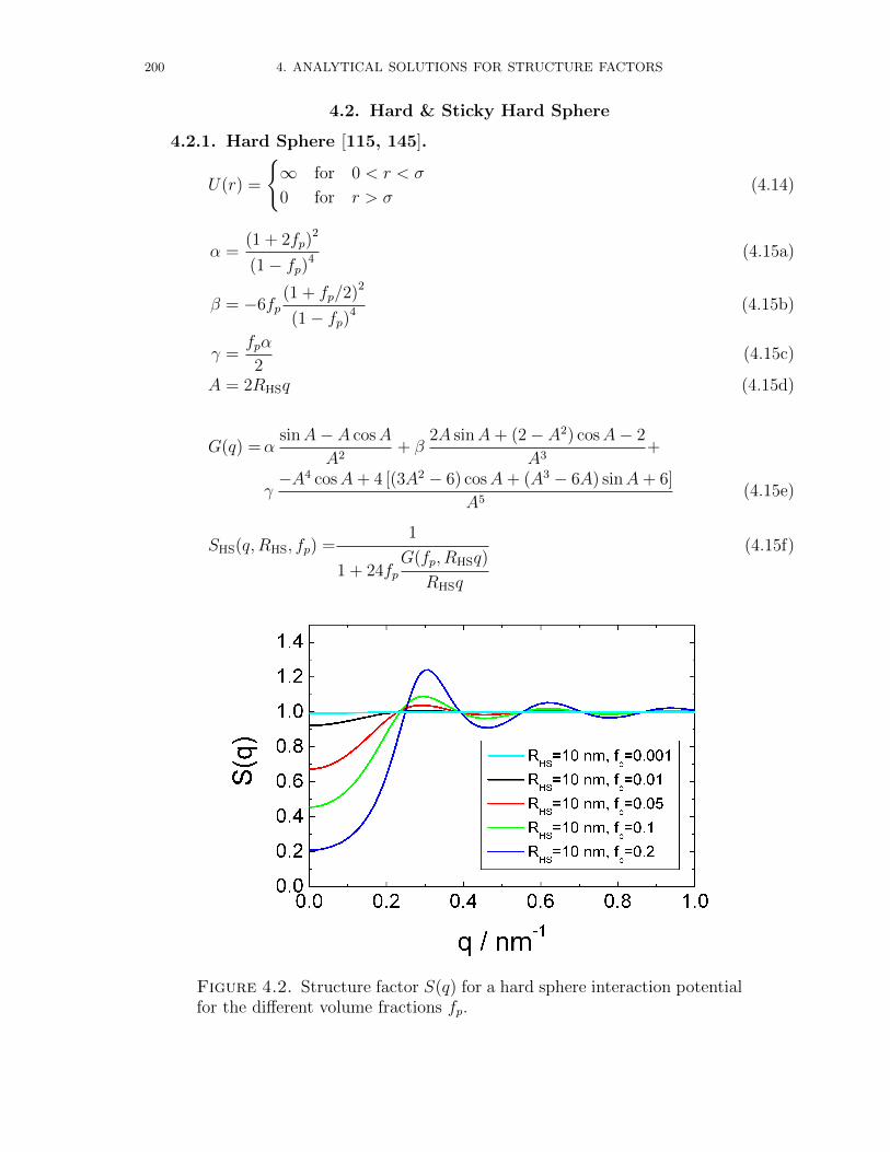
200 4. ANALYTICAL SOLUTIONS FOR STRUCTURE FACTORS
4.2. Hard & Sticky Hard Sphere
4.2.1. Hard Sphere [115, 145].
U(r) =
∞ for 0 < r < σ
0 for r > σ(4.14)
α =(1 + 2fp)
2
(1− fp)4 (4.15a)
β = −6fp(1 + fp/2)2
(1− fp)4 (4.15b)
γ =fpα
2(4.15c)
A = 2RHSq (4.15d)
G(q) =αsinA− A cosA
A2+ β
2A sinA+ (2− A2) cosA− 2
A3+
γ−A4 cosA+ 4 [(3A2 − 6) cosA+ (A3 − 6A) sinA+ 6]
A5(4.15e)
SHS(q, RHS, fp) =1
1 + 24fpG(fp, RHSq)
RHSq
(4.15f)
Figure 4.2. Structure factor S(q) for a hard sphere interaction potentialfor the different volume fractions fp.
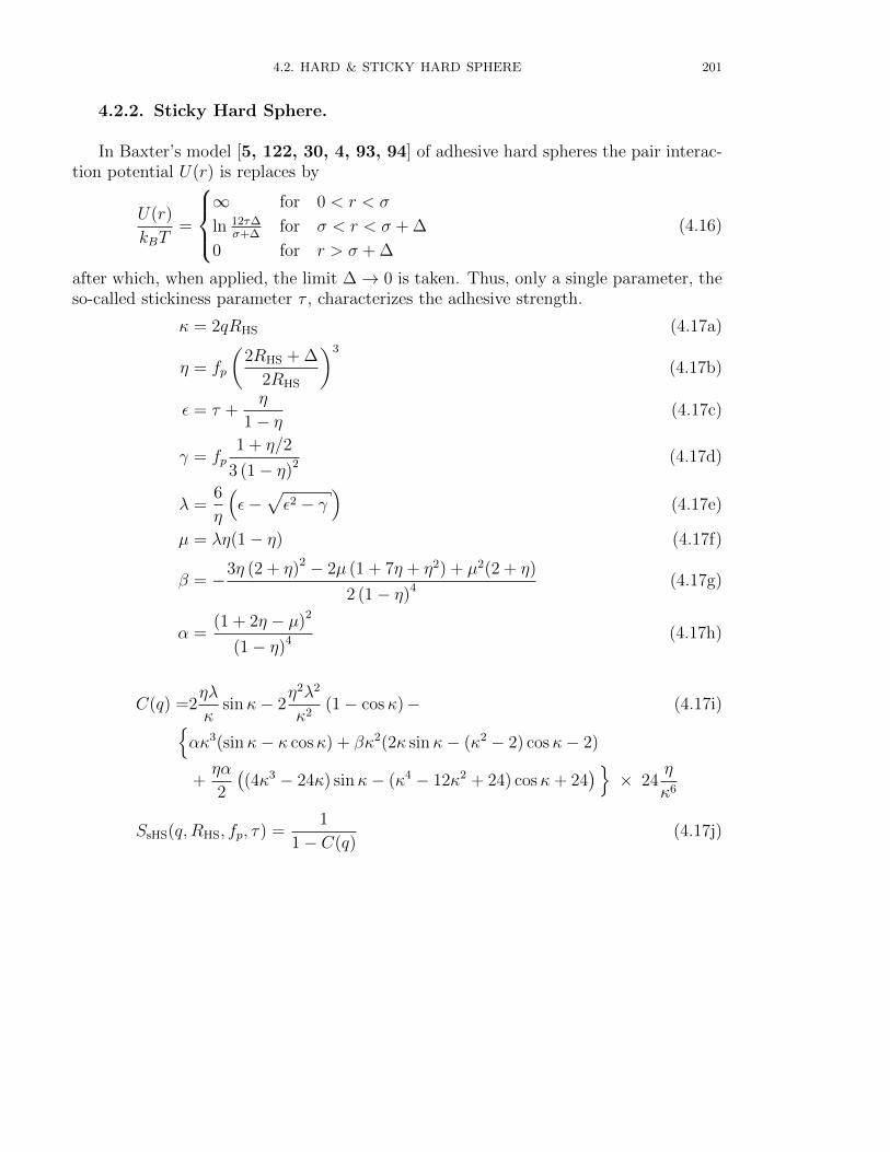
4.2. HARD & STICKY HARD SPHERE 201
4.2.2. Sticky Hard Sphere.
In Baxter’s model [5, 122, 30, 4, 93, 94] of adhesive hard spheres the pair interac-tion potential U(r) is replaces by
U(r)
kBT=
∞ for 0 < r < σ
ln 12τ∆σ+∆
for σ < r < σ + ∆
0 for r > σ + ∆
(4.16)
after which, when applied, the limit ∆→ 0 is taken. Thus, only a single parameter, theso-called stickiness parameter τ , characterizes the adhesive strength.
κ = 2qRHS (4.17a)
η = fp
(2RHS + ∆
2RHS
)3
(4.17b)
ε = τ +η
1− η(4.17c)
γ = fp1 + η/2
3 (1− η)2 (4.17d)
λ =6
η
(ε−
√ε2 − γ
)(4.17e)
µ = λη(1− η) (4.17f)
β = −3η (2 + η)2 − 2µ (1 + 7η + η2) + µ2(2 + η)
2 (1− η)4 (4.17g)
α =(1 + 2η − µ)2
(1− η)4 (4.17h)
C(q) =2ηλ
κsinκ− 2
η2λ2
κ2(1− cosκ)− (4.17i)
ακ3(sinκ− κ cosκ) + βκ2(2κ sinκ− (κ2 − 2) cosκ− 2)
+ηα
2
((4κ3 − 24κ) sinκ− (κ4 − 12κ2 + 24) cosκ+ 24
)× 24
η
κ6
SsHS(q, RHS, fp, τ) =1
1− C(q)(4.17j)

202 4. ANALYTICAL SOLUTIONS FOR STRUCTURE FACTORS
Figure 4.3. Structure factor S(q) for a sticky hard sphere interactionpotential for the different stickiness parameters τ .
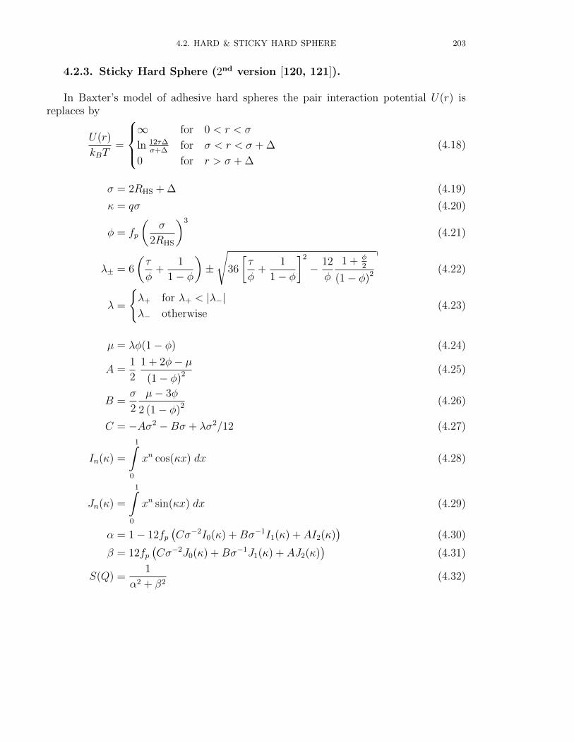
4.2. HARD & STICKY HARD SPHERE 203
4.2.3. Sticky Hard Sphere (2nd version [120, 121]).
In Baxter’s model of adhesive hard spheres the pair interaction potential U(r) isreplaces by
U(r)
kBT=
∞ for 0 < r < σ
ln 12τ∆σ+∆
for σ < r < σ + ∆
0 for r > σ + ∆
(4.18)
σ = 2RHS + ∆ (4.19)
κ = qσ (4.20)
φ = fp
(σ
2RHS
)3
(4.21)
λ± = 6
(τ
φ+
1
1− φ
)±
√36
[τ
φ+
1
1− φ
]2
− 12
φ
1 + φ2
(1− φ)2 (4.22)
λ =
λ+ for λ+ < |λ−|λ− otherwise
(4.23)
µ = λφ(1− φ) (4.24)
A =1
2
1 + 2φ− µ(1− φ)2 (4.25)
B =σ
2
µ− 3φ
2 (1− φ)2 (4.26)
C = −Aσ2 −Bσ + λσ2/12 (4.27)
In(κ) =
1∫0
xn cos(κx) dx (4.28)
Jn(κ) =
1∫0
xn sin(κx) dx (4.29)
α = 1− 12fp(Cσ−2I0(κ) +Bσ−1I1(κ) + AI2(κ)
)(4.30)
β = 12fp(Cσ−2J0(κ) +Bσ−1J1(κ) + AJ2(κ)
)(4.31)
S(Q) =1
α2 + β2(4.32)

204 4. ANALYTICAL SOLUTIONS FOR STRUCTURE FACTORS
Figure 4.4. Structure factor S(q) for a sticky hard sphere interactionpotential for the different stickiness parameters τ .
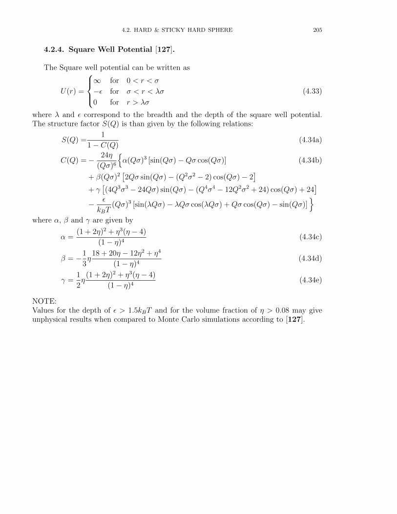
4.2. HARD & STICKY HARD SPHERE 205
4.2.4. Square Well Potential [127].
The Square well potential can be written as
U(r) =
∞ for 0 < r < σ
−ε for σ < r < λσ
0 for r > λσ
(4.33)
where λ and ε correspond to the breadth and the depth of the square well potential.The structure factor S(Q) is than given by the following relations:
S(Q) =1
1− C(Q)(4.34a)
C(Q) =− 24η
(Qσ)6
α(Qσ)3 [sin(Qσ)−Qσ cos(Qσ)] (4.34b)
+ β(Qσ)2[2Qσ sin(Qσ)− (Q2σ2 − 2) cos(Qσ)− 2
]+ γ
[(4Q3σ3 − 24Qσ) sin(Qσ)− (Q4σ4 − 12Q2σ2 + 24) cos(Qσ) + 24
]− ε
kBT(Qσ)3 [sin(λQσ)− λQσ cos(λQσ) +Qσ cos(Qσ)− sin(Qσ)]
where α, β and γ are given by
α =(1 + 2η)2 + η3(η − 4)
(1− η)4(4.34c)
β = −1
3η
18 + 20η − 12η2 + η4
(1− η)4(4.34d)
γ =1
2η
(1 + 2η)2 + η3(η − 4)
(1− η)4(4.34e)
NOTE:Values for the depth of ε > 1.5kBT and for the volume fraction of η > 0.08 may giveunphysical results when compared to Monte Carlo simulations according to [127].
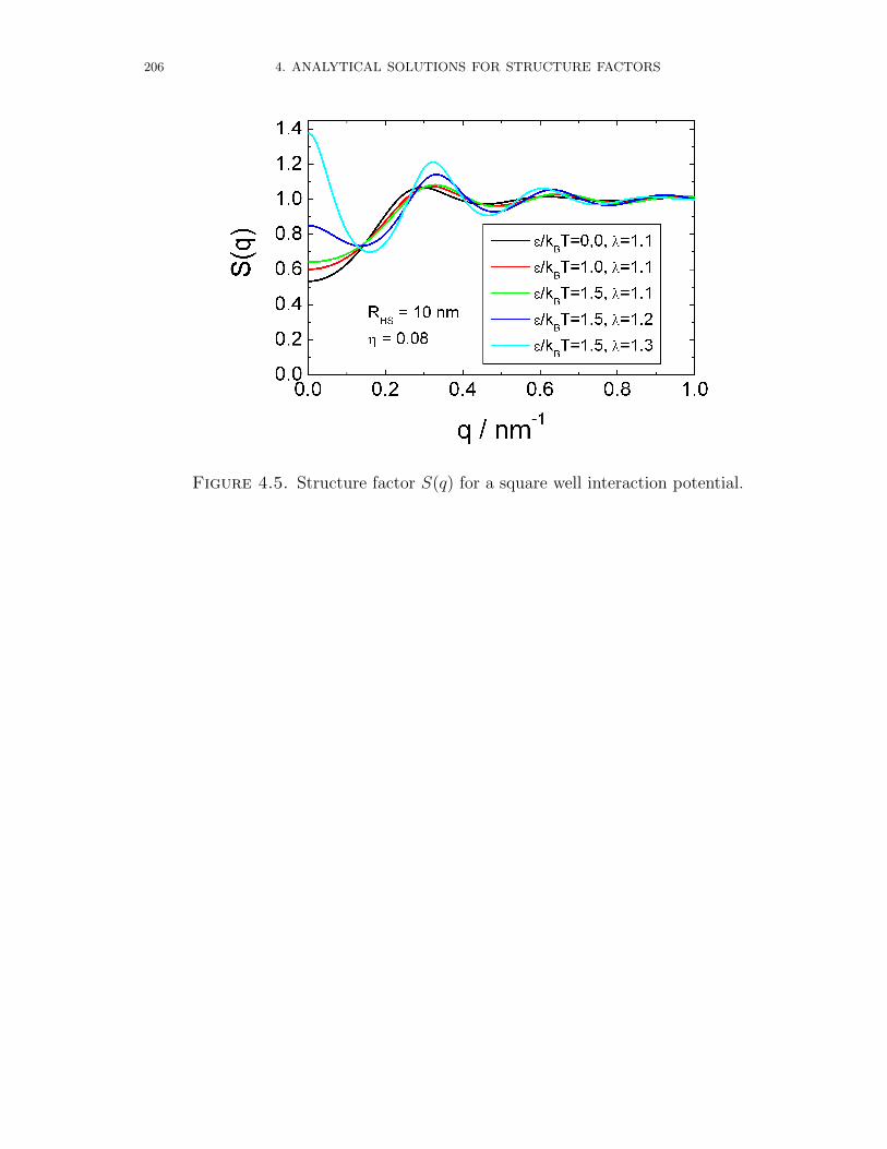
206 4. ANALYTICAL SOLUTIONS FOR STRUCTURE FACTORS
Figure 4.5. Structure factor S(q) for a square well interaction potential.
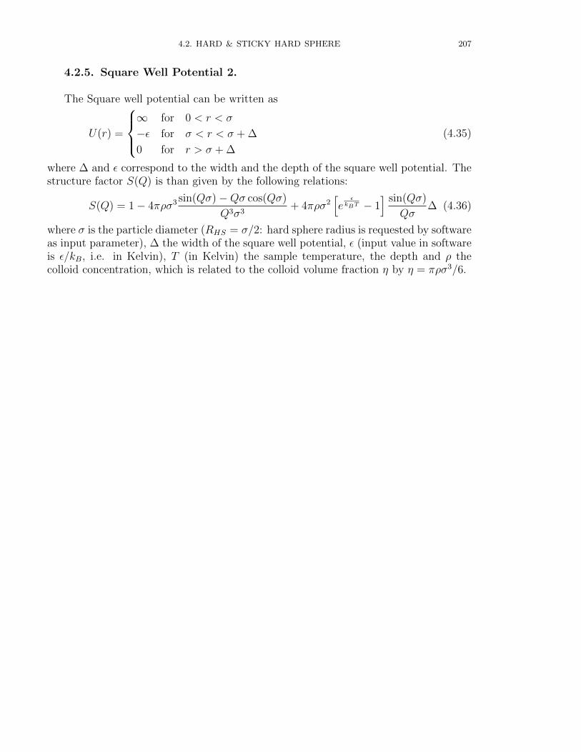
4.2. HARD & STICKY HARD SPHERE 207
4.2.5. Square Well Potential 2.
The Square well potential can be written as
U(r) =
∞ for 0 < r < σ
−ε for σ < r < σ + ∆
0 for r > σ + ∆
(4.35)
where ∆ and ε correspond to the width and the depth of the square well potential. Thestructure factor S(Q) is than given by the following relations:
S(Q) = 1− 4πρσ3 sin(Qσ)−Qσ cos(Qσ)
Q3σ3+ 4πρσ2
[e
εkBT − 1
] sin(Qσ)
Qσ∆ (4.36)
where σ is the particle diameter (RHS = σ/2: hard sphere radius is requested by softwareas input parameter), ∆ the width of the square well potential, ε (input value in softwareis ε/kB, i.e. in Kelvin), T (in Kelvin) the sample temperature, the depth and ρ thecolloid concentration, which is related to the colloid volume fraction η by η = πρσ3/6.

208 4. ANALYTICAL SOLUTIONS FOR STRUCTURE FACTORS
4.3. Multi Lamellar Structures [107, 44]
4.3.1. Multi-Lamellar Structures, Thermal Disorder.
Figure 4.6. Thermal disorder, considering fluctuations of flat layersaround well defined and evenly spaced equilibrium positions.
The first type describes thermal disorder (TD) caused by small fluctuations of thebilayers around well defined mean layer positions of equal separation (Fig. 4.6). In sucha crystal lattice the long-range order is preserved and the structure factor for a singledomain of size L = Nd is identical to that of a perfect finite crystal multiplied by thewell known Debye-Waller temperature factor, where ∆ = 〈(dk − d)2〉 denotes the meansquare fluctuations of the bilayers. As shown in Fig. 4.6, STD(Q) is characterized bya set of Bragg peaks of equal width, the diffraction order amplitudes of which decreaseexponentially with the Debye-Waller factor. The lost intensity is found as a diffusebackground scattering, which increases to the limit of N for large Q.
STD(Q,N, d,∆, Ndiff) = Ndiff +N+2σ∑
Nk=N−2σ
xkSk,TD (4.37)
with
Sk,TD =
(Nk + 2 exp
(−Q
2∆2
2
)Nk−1∑m=1
(Nk −m) cos(mQd)
)(4.38)
Ndiff accounts for an additional diffuse background, due to a number of uncorrelatedscattering bilayers in STD(Q,N, d,∆, Ndiff), which is not included in the TD theory. Itsorigin is attributed to bilayers with strong lattice defects or unilamellar vesicles, whichdisplay neither short-range nor (quasi-) long-range order.
The structure factors Sk,TD(Q) with low, but fixed stacking numbers N show os-cillations at low Q (as can be seen in Fig. 4.6), but no such oscillations are found inexperimental data. This can be understood as the consequence of polydispersity in the
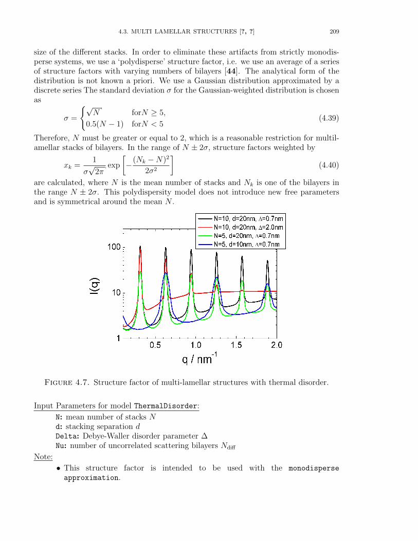
4.3. MULTI LAMELLAR STRUCTURES [?, ?] 209
size of the different stacks. In order to eliminate these artifacts from strictly monodis-perse systems, we use a ‘polydisperse’ structure factor, i.e. we use an average of a seriesof structure factors with varying numbers of bilayers [44]. The analytical form of thedistribution is not known a priori. We use a Gaussian distribution approximated by adiscrete series The standard deviation σ for the Gaussian-weighted distribution is chosenas
σ =
√N forN ≥ 5,
0.5(N − 1) forN < 5(4.39)
Therefore, N must be greater or equal to 2, which is a reasonable restriction for multil-amellar stacks of bilayers. In the range of N ± 2σ, structure factors weighted by
xk =1
σ√
2πexp
[−(Nk −N)2
2σ2
](4.40)
are calculated, where N is the mean number of stacks and Nk is one of the bilayers inthe range N ± 2σ. This polydispersity model does not introduce new free parametersand is symmetrical around the mean N .
Figure 4.7. Structure factor of multi-lamellar structures with thermal disorder.
Input Parameters for model ThermalDisorder:
N: mean number of stacks Nd: stacking separation dDelta: Debye-Waller disorder parameter ∆Nu: number of uncorrelated scattering bilayers Ndiff
Note:
• This structure factor is intended to be used with the monodisperse
approximation.
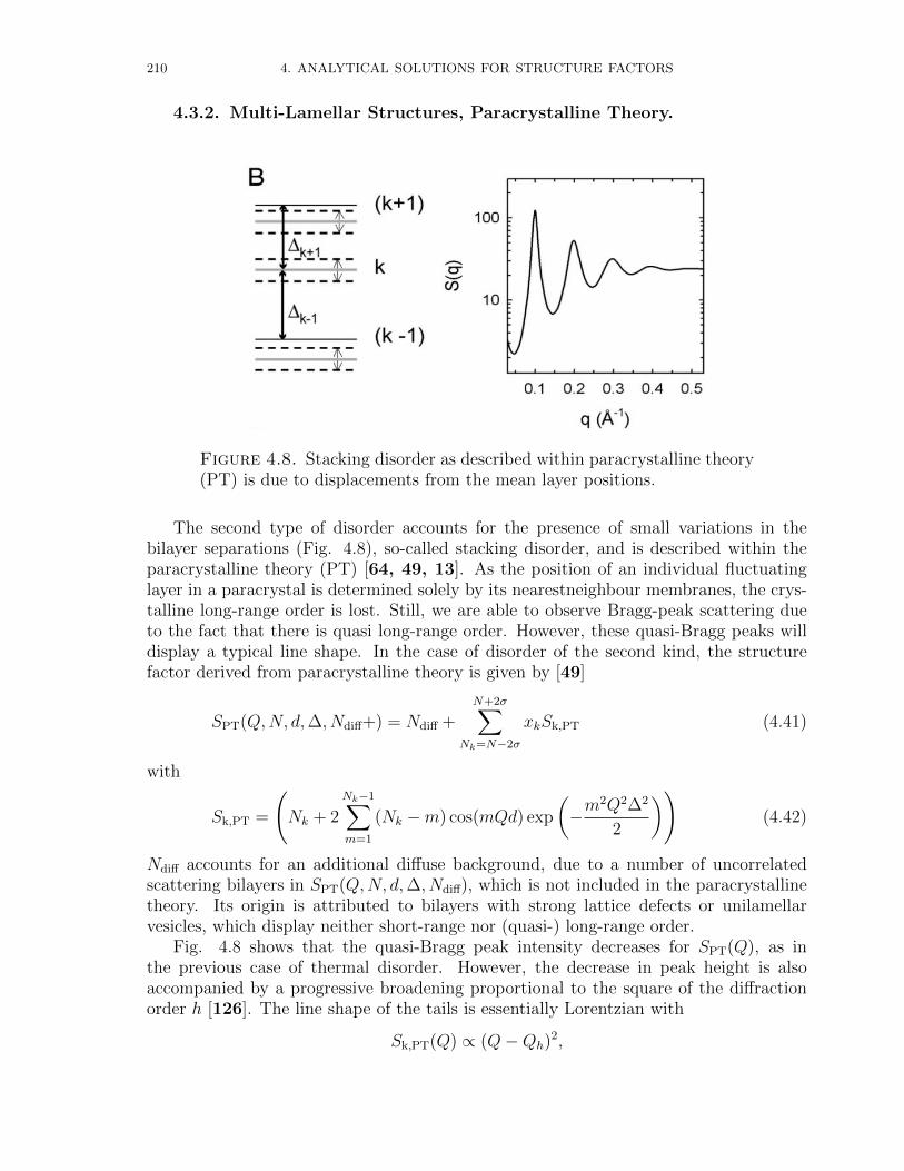
210 4. ANALYTICAL SOLUTIONS FOR STRUCTURE FACTORS
4.3.2. Multi-Lamellar Structures, Paracrystalline Theory.
Figure 4.8. Stacking disorder as described within paracrystalline theory(PT) is due to displacements from the mean layer positions.
The second type of disorder accounts for the presence of small variations in thebilayer separations (Fig. 4.8), so-called stacking disorder, and is described within theparacrystalline theory (PT) [64, 49, 13]. As the position of an individual fluctuatinglayer in a paracrystal is determined solely by its nearestneighbour membranes, the crys-talline long-range order is lost. Still, we are able to observe Bragg-peak scattering dueto the fact that there is quasi long-range order. However, these quasi-Bragg peaks willdisplay a typical line shape. In the case of disorder of the second kind, the structurefactor derived from paracrystalline theory is given by [49]
SPT(Q,N, d,∆, Ndiff+) = Ndiff +N+2σ∑
Nk=N−2σ
xkSk,PT (4.41)
with
Sk,PT =
(Nk + 2
Nk−1∑m=1
(Nk −m) cos(mQd) exp
(−m
2Q2∆2
2
))(4.42)
Ndiff accounts for an additional diffuse background, due to a number of uncorrelatedscattering bilayers in SPT(Q,N, d,∆, Ndiff), which is not included in the paracrystallinetheory. Its origin is attributed to bilayers with strong lattice defects or unilamellarvesicles, which display neither short-range nor (quasi-) long-range order.
Fig. 4.8 shows that the quasi-Bragg peak intensity decreases for SPT(Q), as inthe previous case of thermal disorder. However, the decrease in peak height is alsoaccompanied by a progressive broadening proportional to the square of the diffractionorder h [126]. The line shape of the tails is essentially Lorentzian with
Sk,PT(Q) ∝ (Q−Qh)2,
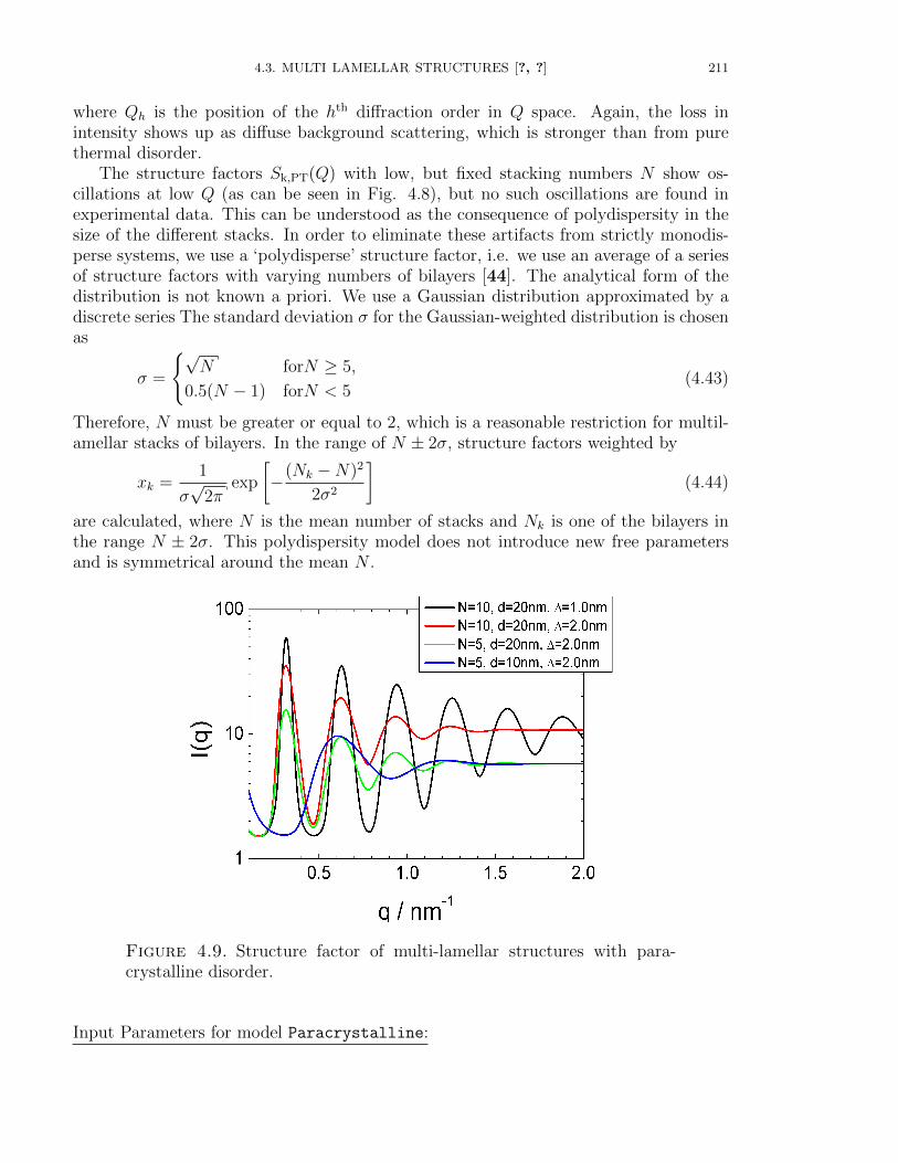
4.3. MULTI LAMELLAR STRUCTURES [?, ?] 211
where Qh is the position of the hth diffraction order in Q space. Again, the loss inintensity shows up as diffuse background scattering, which is stronger than from purethermal disorder.
The structure factors Sk,PT(Q) with low, but fixed stacking numbers N show os-cillations at low Q (as can be seen in Fig. 4.8), but no such oscillations are found inexperimental data. This can be understood as the consequence of polydispersity in thesize of the different stacks. In order to eliminate these artifacts from strictly monodis-perse systems, we use a ‘polydisperse’ structure factor, i.e. we use an average of a seriesof structure factors with varying numbers of bilayers [44]. The analytical form of thedistribution is not known a priori. We use a Gaussian distribution approximated by adiscrete series The standard deviation σ for the Gaussian-weighted distribution is chosenas
σ =
√N forN ≥ 5,
0.5(N − 1) forN < 5(4.43)
Therefore, N must be greater or equal to 2, which is a reasonable restriction for multil-amellar stacks of bilayers. In the range of N ± 2σ, structure factors weighted by
xk =1
σ√
2πexp
[−(Nk −N)2
2σ2
](4.44)
are calculated, where N is the mean number of stacks and Nk is one of the bilayers inthe range N ± 2σ. This polydispersity model does not introduce new free parametersand is symmetrical around the mean N .
Figure 4.9. Structure factor of multi-lamellar structures with para-crystalline disorder.
Input Parameters for model Paracrystalline:
212 4. ANALYTICAL SOLUTIONS FOR STRUCTURE FACTORS
N: mean number of stacks Nd: stacking separation dDelta: stacking disorder parameter ∆Nu: number of uncorrelated scattering bilayers Ndiff
Note:
• This structure factor is intended to be used with the monodisperse
approximation.
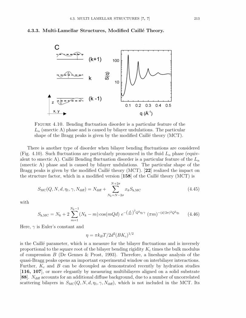
4.3. MULTI LAMELLAR STRUCTURES [?, ?] 213
4.3.3. Multi-Lamellar Structures, Modified Caille Theory.
Figure 4.10. Bending fluctuation disorder is a particular feature of theLα (smectic A) phase and is caused by bilayer undulations. The particularshape of the Bragg peaks is given by the modified Caille theory (MCT).
There is another type of disorder when bilayer bending fluctuations are considered(Fig. 4.10). Such fluctuations are particularly pronounced in the fluid Lα phase (equiv-alent to smectic A). Caille Bending fluctuation disorder is a particular feature of the Lα(smectic A) phase and is caused by bilayer undulations. The particular shape of theBragg peaks is given by the modified Caille theory (MCT). [22] realized the impact onthe structure factor, which in a modified version [158] of the Caille theory (MCT) is
SMC(Q,N, d, η1, γ,Ndiff) = Ndiff +N+2σ∑
Nk=N−2σ
xkSk,MC (4.45)
with
Sk,MC = Nk + 2
Nk−1∑m=1
(Nk −m) cos(mQd) e−( d2π )
2Q2η1γ (πm)−(d/2π)2Q2η1 (4.46)
Here, γ is Euler’s constant and
η = πkBT/2d2(BKc)
1/2
is the Caille parameter, which is a measure for the bilayer fluctuations and is inverselyproportional to the square root of the bilayer bending rigidity Kc times the bulk modulusof compression B (De Gennes & Prost, 1993). Therefore, a lineshape analysis of thequasi-Bragg peaks opens an important experimental window on interbilayer interactions.Further, Kc and B can be decoupled as demonstrated recently by hydration studies[116, 107], or more elegantly by measuring multibilayers aligned on a solid substrate[88]. Ndiff accounts for an additional diffuse background, due to a number of uncorrelatedscattering bilayers in SMC(Q,N, d, η1, γ,Ndiff), which is not included in the MCT. Its
214 4. ANALYTICAL SOLUTIONS FOR STRUCTURE FACTORS
origin is attributed to bilayers with strong lattice defects or unilamellar vesicles, whichdisplay neither short-range nor (quasi-) long-range order.
Fig. 4.10 shows a typical example of Sk,MCT(Q), which is similar to SPT(Q) withrespect to the progressive decrease in peak height and increase in peak width, but whichdiffers significantly in line shape as
Sk,MCT ∝ (Q−Qh)−1+ηh2
for randomly oriented scattering domains [124, 158].The structure factors Sk,MCT(Q) with low, but fixed stacking numbers N show os-
cillations at low Q (as can be seen in Fig. 4.10), but no such oscillations are found inexperimental data. This can be understood as the consequence of polydispersity in thesize of the different stacks. In order to eliminate these artifacts from strictly monodis-perse systems, we use a ‘polydisperse’ structure factor, i.e. we use an average of a seriesof structure factors with varying numbers of bilayers [44]. The analytical form of thedistribution is not known a priori. We use a Gaussian distribution approximated by adiscrete series The standard deviation σ for the Gaussian-weighted distribution is chosenas
σ =
√N forN ≥ 5,
0.5(N − 1) forN < 5(4.47)
Therefore, N must be greater or equal to 2, which is a reasonable restriction for multil-amellar stacks of bilayers. In the range of N ± 2σ, structure factors weighted by
xk =1
σ√
2πexp
[−(Nk −N)2
2σ2
](4.48)
are calculated, where N is the mean number of stacks and Nk is one of the bilayers inthe range N ± 2σ. This polydispersity model does not introduce new free parametersand is symmetrical around the mean N .
Input Parameters for model ModifiedCaile:
N: mean number of stacks Nd: stacking separation deta: the Caille parameter η is a measure for the bilayer fluctuations and inversely
proportional to the square root of the bilayer bending rigidityNu: number of uncorrelated scattering bilayers Ndiff
Note:
• This structure factor is intended to be used with the monodisperse
approximation.
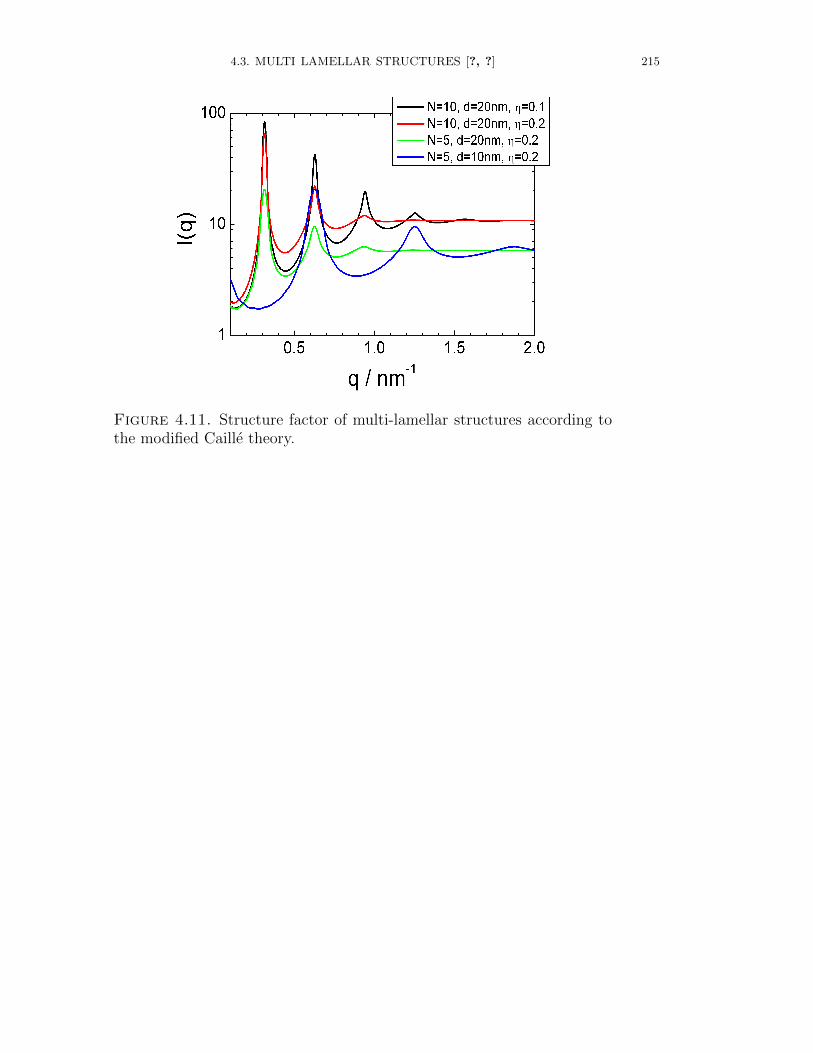
4.3. MULTI LAMELLAR STRUCTURES [?, ?] 215
Figure 4.11. Structure factor of multi-lamellar structures according tothe modified Caille theory.
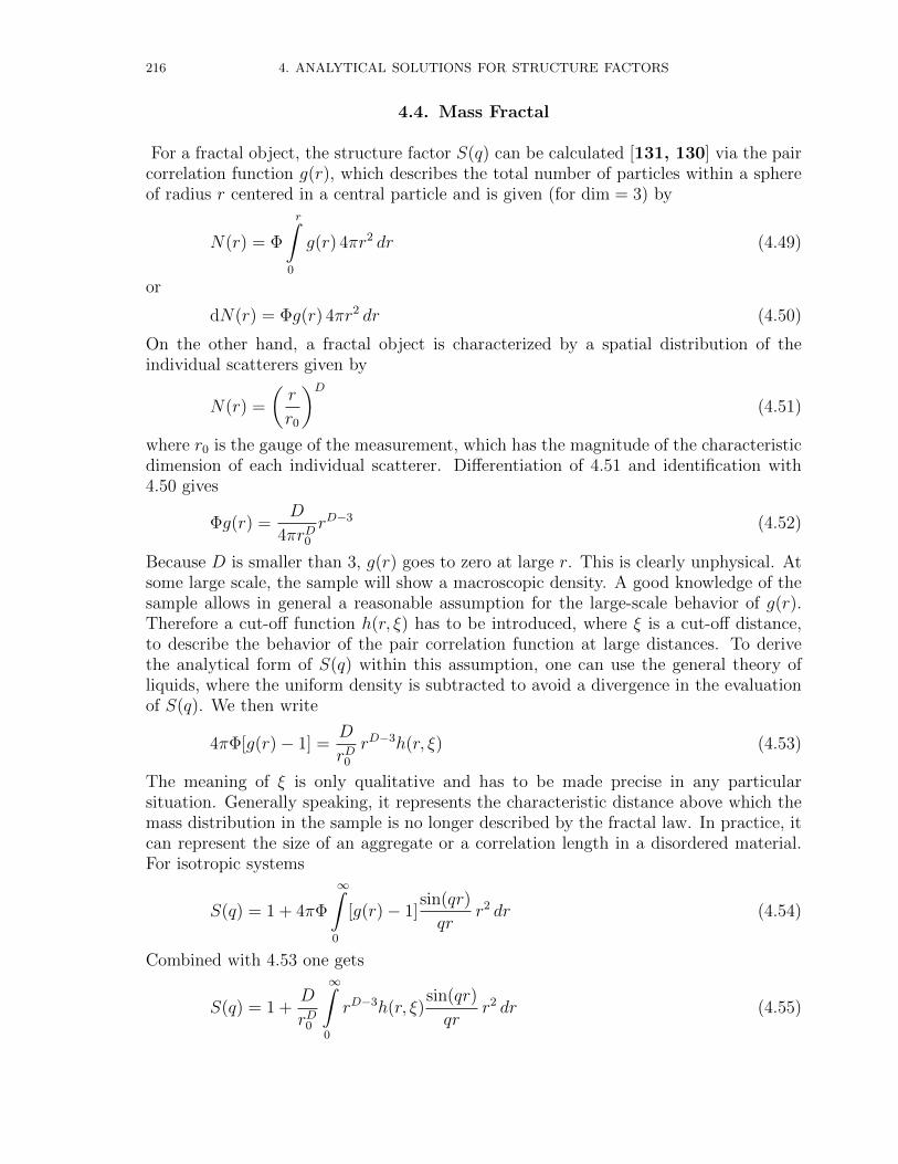
216 4. ANALYTICAL SOLUTIONS FOR STRUCTURE FACTORS
4.4. Mass Fractal
For a fractal object, the structure factor S(q) can be calculated [131, 130] via the paircorrelation function g(r), which describes the total number of particles within a sphereof radius r centered in a central particle and is given (for dim = 3) by
N(r) = Φ
r∫0
g(r) 4πr2 dr (4.49)
or
dN(r) = Φg(r) 4πr2 dr (4.50)
On the other hand, a fractal object is characterized by a spatial distribution of theindividual scatterers given by
N(r) =
(r
r0
)D(4.51)
where r0 is the gauge of the measurement, which has the magnitude of the characteristicdimension of each individual scatterer. Differentiation of 4.51 and identification with4.50 gives
Φg(r) =D
4πrD0rD−3 (4.52)
Because D is smaller than 3, g(r) goes to zero at large r. This is clearly unphysical. Atsome large scale, the sample will show a macroscopic density. A good knowledge of thesample allows in general a reasonable assumption for the large-scale behavior of g(r).Therefore a cut-off function h(r, ξ) has to be introduced, where ξ is a cut-off distance,to describe the behavior of the pair correlation function at large distances. To derivethe analytical form of S(q) within this assumption, one can use the general theory ofliquids, where the uniform density is subtracted to avoid a divergence in the evaluationof S(q). We then write
4πΦ[g(r)− 1] =D
rD0rD−3h(r, ξ) (4.53)
The meaning of ξ is only qualitative and has to be made precise in any particularsituation. Generally speaking, it represents the characteristic distance above which themass distribution in the sample is no longer described by the fractal law. In practice, itcan represent the size of an aggregate or a correlation length in a disordered material.For isotropic systems
S(q) = 1 + 4πΦ
∞∫0
[g(r)− 1]sin(qr)
qrr2 dr (4.54)
Combined with 4.53 one gets
S(q) = 1 +D
rD0
∞∫0
rD−3h(r, ξ)sin(qr)
qrr2 dr (4.55)
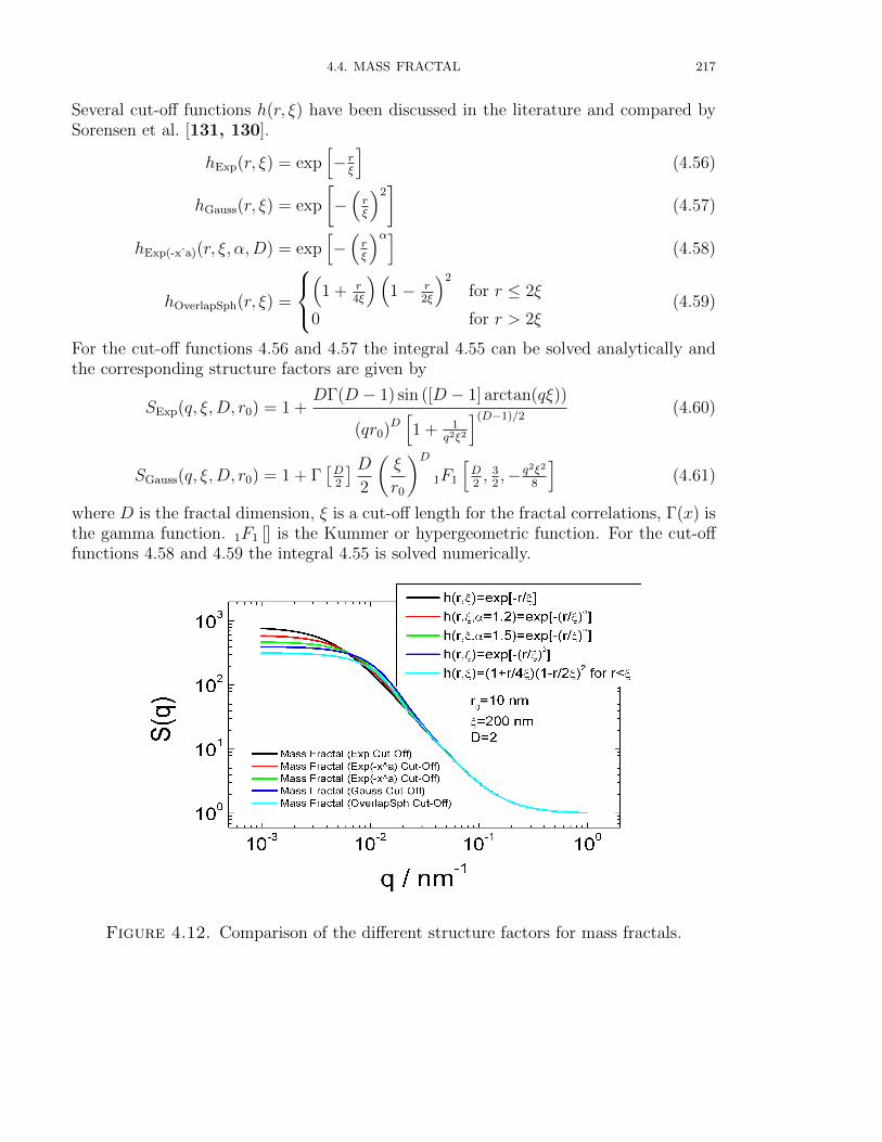
4.4. MASS FRACTAL 217
Several cut-off functions h(r, ξ) have been discussed in the literature and compared bySorensen et al. [131, 130].
hExp(r, ξ) = exp[− rξ
](4.56)
hGauss(r, ξ) = exp
[−(rξ
)2]
(4.57)
hExp(-x a)(r, ξ, α,D) = exp[−(rξ
)α](4.58)
hOverlapSph(r, ξ) =
(
1 + r4ξ
)(1− r
2ξ
)2
for r ≤ 2ξ
0 for r > 2ξ(4.59)
For the cut-off functions 4.56 and 4.57 the integral 4.55 can be solved analytically andthe corresponding structure factors are given by
SExp(q, ξ,D, r0) = 1 +DΓ(D − 1) sin ([D − 1] arctan(qξ))
(qr0)D[1 + 1
q2ξ2
](D−1)/2(4.60)
SGauss(q, ξ,D, r0) = 1 + Γ[D2
] D2
(ξ
r0
)D1F1
[D2, 3
2,− q2ξ2
8
](4.61)
where D is the fractal dimension, ξ is a cut-off length for the fractal correlations, Γ(x) isthe gamma function. 1F1 [] is the Kummer or hypergeometric function. For the cut-offfunctions 4.58 and 4.59 the integral 4.55 is solved numerically.
Figure 4.12. Comparison of the different structure factors for mass fractals.
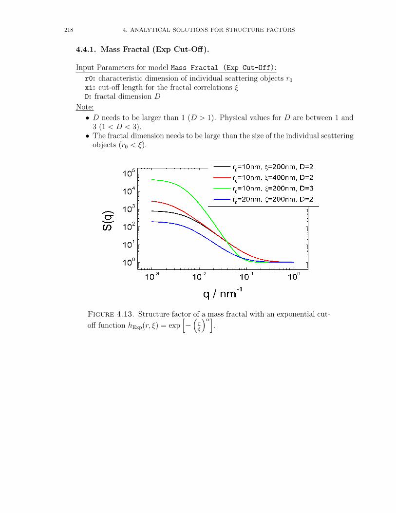
218 4. ANALYTICAL SOLUTIONS FOR STRUCTURE FACTORS
4.4.1. Mass Fractal (Exp Cut-Off).
Input Parameters for model Mass Fractal (Exp Cut-Off):
r0: characteristic dimension of individual scattering objects r0
xi: cut-off length for the fractal correlations ξD: fractal dimension D
Note:
• D needs to be larger than 1 (D > 1). Physical values for D are between 1 and3 (1 < D < 3).• The fractal dimension needs to be large than the size of the individual scattering
objects (r0 < ξ).
Figure 4.13. Structure factor of a mass fractal with an exponential cut-
off function hExp(r, ξ) = exp[−(rξ
)α].
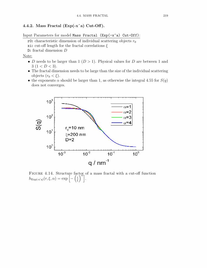
4.4. MASS FRACTAL 219
4.4.2. Mass Fractal (Exp(-xˆa) Cut-Off).
Input Parameters for model Mass Fractal (Exp(-x^a) Cut-Off):
r0: characteristic dimension of individual scattering objects r0
xi: cut-off length for the fractal correlations ξD: fractal dimension D
Note:
• D needs to be larger than 1 (D > 1). Physical values for D are between 1 and3 (1 < D < 3).• The fractal dimension needs to be large than the size of the individual scattering
objects (r0 < ξ).• the exponents α should be larger than 1, as otherwise the integral 4.55 for S(q)
does not converges.
Figure 4.14. Structure factor of a mass fractal with a cut-off function
hExp(-x a)(r, ξ, α) = exp[−(rξ
)α].
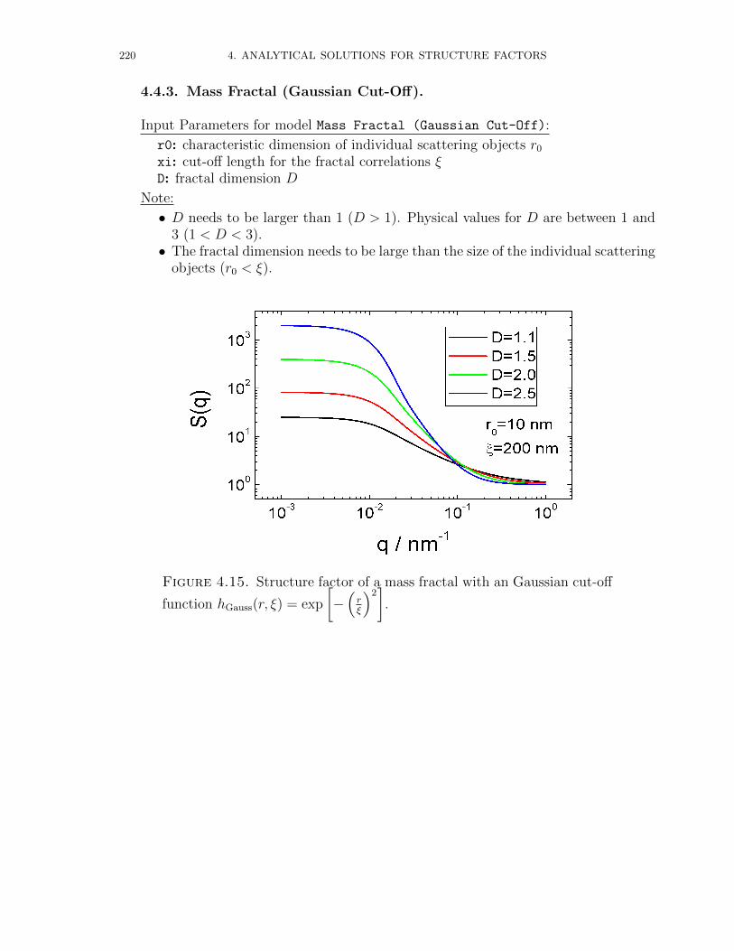
220 4. ANALYTICAL SOLUTIONS FOR STRUCTURE FACTORS
4.4.3. Mass Fractal (Gaussian Cut-Off).
Input Parameters for model Mass Fractal (Gaussian Cut-Off):
r0: characteristic dimension of individual scattering objects r0
xi: cut-off length for the fractal correlations ξD: fractal dimension D
Note:
• D needs to be larger than 1 (D > 1). Physical values for D are between 1 and3 (1 < D < 3).• The fractal dimension needs to be large than the size of the individual scattering
objects (r0 < ξ).
Figure 4.15. Structure factor of a mass fractal with an Gaussian cut-off
function hGauss(r, ξ) = exp
[−(rξ
)2].
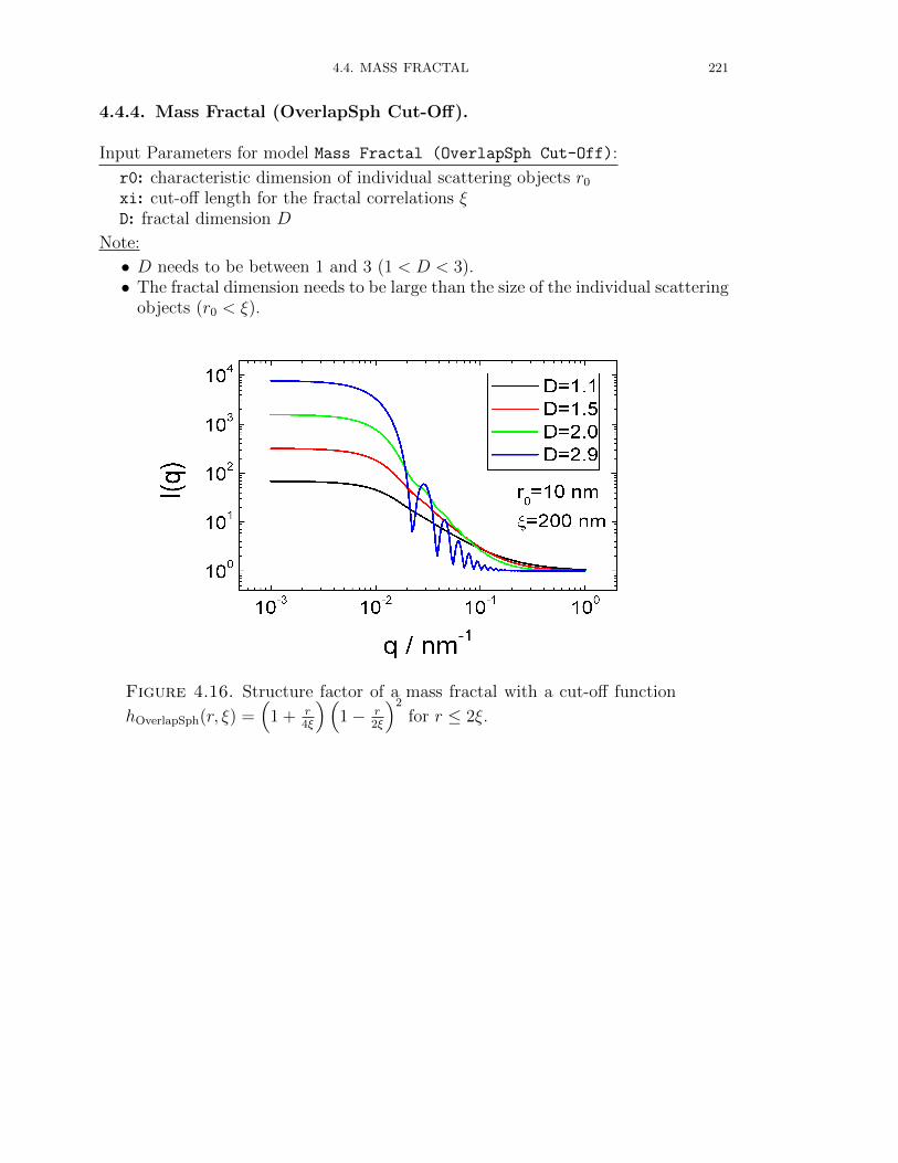
4.4. MASS FRACTAL 221
4.4.4. Mass Fractal (OverlapSph Cut-Off).
Input Parameters for model Mass Fractal (OverlapSph Cut-Off):
r0: characteristic dimension of individual scattering objects r0
xi: cut-off length for the fractal correlations ξD: fractal dimension D
Note:
• D needs to be between 1 and 3 (1 < D < 3).• The fractal dimension needs to be large than the size of the individual scattering
objects (r0 < ξ).
Figure 4.16. Structure factor of a mass fractal with a cut-off function
hOverlapSph(r, ξ) =(
1 + r4ξ
)(1− r
2ξ
)2
for r ≤ 2ξ.
222 4. ANALYTICAL SOLUTIONS FOR STRUCTURE FACTORS
4.5. Other Structure Factors
4.5.1. Hayter-Penfold RMSA [57, 55]. This is the structure factor for a systemof charged, spheroidal objects in a dielectric medium. When combined with an appro-priate form factor (such as sphere, core+shell, ellipsoid etc.), this allows for inclusion ofthe interparticle interference effects due to screened coulomb repulsion between chargedparticles. The salt concentration, is used to compute the ionic strength of the solutionwhich in turn is used to compute the Debye screening length. At present there is noprovision for entering the ionic strength directly nor for use of any multivalent salts.The counterions are also assumed to be monovalent.
Input Parameters for model Hayter Penfold RMSA:
RHS: hard sphere radius RHS of particles in [nm].Z: charge of particle in units of the charge of an electron e =?1.60217653× 10?19Ceta: volume fraction η of particlesT: sample temperature T in Kelvinsalt: monovalent salt concentration in [M]eps r: dielectric constant εr of solvent

4.5. OTHER STRUCTURE FACTORS 223
4.5.2. MacroIon.
ETA = volume fraction (4.62a)
AK = κσ = inv. screening length times diameter (4.62b)
κ =√e2/(εε0kBT ) ∗ (ρc + 2ρs) (4.62c)
ρc = density of counterions = ρcolloidsZ (4.62d)
ρs = density of salt cations or anions (4.62e)
GEK = charge2/(πkBTεε0σ(2 + AK)2) (4.62f)
charge = Ladung eines Kolloids = eZ (4.62g)
S = ETA1./3 = scaling factor for rescaled MSA (RMSA) (4.62h)
GAMK = 2 ∗ S ∗GEK ∗ exp(AK − AK/S). (4.62i)

224 4. ANALYTICAL SOLUTIONS FOR STRUCTURE FACTORS
4.5.3. Critical Scattering.
Scrit(Q) = 1 +κ
1 + ζ2Q2(4.63)
ζ: correlation length, κ: scaling factor
4.5.4. Correlation Hole.
Scorr. hole(Q, h, η) = 1 + ηΦ(Qh) (4.64)
Φ(x) = 3 sin(x)−x cos(x)x3 η: volume fraction, h: hole radius
4.5.5. Random Distribution Model.
SRDM(Q) =1
1 + 8Vca/Vpε
Φ(x)(4.65)
x = 2QRca
Vca = 43πR3
ca
Vp = 43πR3/fp
Φ(x) = 3 sin(x)−x cos(x)x3
4.5.6. Local Order Model.
SLOM(Q) = 1 + 4sin(QD)
QD− zΦ(x); (4.66)
x = αQD
Φ(x) = 3 sin(x)−x cos(x)x3
4.5.7. Cylinder(PRISM).
SCyl,PRISM =1
1 + νCqP15
(4.67)
x = 2QR
xP15 = Q(L− 2R)
P15 = 2Si(xP15)
xP15
− 4sin2(xP15/2)
x2P15
Cq = 3sin(x)− x cos(x)
x3
4.5. OTHER STRUCTURE FACTORS 225
4.5.8. Voigt Peak.
In spectroscopy, the Voigt profile is a spectral line profile named after WoldemarVoigt and found in all branches of spectroscopy in which a spectral line is broadened bytwo types of mechanisms, one of which alone would produce a Doppler profile, and theother of which would produce a Lorentzian profile. All normalized line profiles can beconsidered to be probability distributions. The Doppler profile is essentially a normaldistribution and a Lorentzian profile is essentially a Cauchy distribution. Without lossof generality, we can consider only centered profiles which peak at zero. The Voigt profileis then the convolution of a Lorentzian profile and a Doppler profile:
V (x|σ, γ) =
∞∫∞
D(x′|σ)L(x− x′|γ) dx′ (4.68a)
where x is frequency from line center, D(x|σ) is the centered Doppler profile:
D(x|σ) =e−x
2/2σ2
σ√
2π(4.68b)
and L(x|γ) is the centered Lorentzian profile:
L(x|γ) =γ
π(x2 + γ2). (4.68c)
The defining integral can be evaluated as:
V (x) =<[w(z)]
σ√
2π(4.68d)
where <[w(z)] is the real part of the complex error function of z and
z =x+ iγ
σ√
2(4.68e)
SVoigt(Q,Qm, A, σ, γ, c0) = A V (Q−Qm|σ, γ) + c0 (4.68f)

CHAPTER 5
Numerical solutions of the Ornstein Zernike equations
During an internship project in summer 2013 Evgeniy Ponomarev has implementedthe core routine for solving the Ornstein Zernike equations. This algorithm numericallycalculates structure factors S(q), radial distribution functions g(r) and direct correlationfunctions c(r) of a systems with known pair interaction potential U(r).
5.1. Background
The central part of this package is iterative solution of Ornstein-Zernike equation[105]. The theoretical background can be found in great detail in [102, 58, 54, 16, 21,80]. The Ornstein-Zernike equation reads
h(r12) = c(r12) +
∫c(r13)ρ(r3)h(r32)dr3 + · · · (5.1)
where h(r12) is the total correlation function, c(r12) the direct correlation function (directeffect of particle 1 on particle 2), c(r13) the in direct correlation function describing theeffect of particle 1 on particle 3 which influences particle 2, and ρ the particle numberdensity of the colloids, molecules, or atoms that form the liquid. If the fluid is uniformand isotropic, the OrnsteinZernike relation becomes
h(r) = c(r) + ρ
∫c(|r− r′|)h(r′)dr′ (5.2)
= c(r) + γ(r) (5.3)
The basic idea of this equation is that total correlation between positions of two particlesis a combination of their direct and indirect (through neighboring particles) interactions.The first contribution to h(r) is the direct correlation function c(r) that represents thecorrelation between a particle of a pair with its closest neighbor separated by a distancer. The second contribution is the indirect correlation function γ(r), which represents thecorrelation between the selected particle of the pair with the rest of the fluid constituents.
g(r) is known as the radial or pair distribution function, which measures the proba-bility that given a particle at the origin, another particle of the fluid can be found at adistance r from it. When the distance separating a pair of particles tends to infinity, thecorrelations vanish and g(r) tends to 1. This means that the total correlation functiondefined as h(r) = g(r)− 1 tends to 0. The Fourier transform F of g(r) and h(r) aredirectly related to the structure factor S(q) that is experimentally measurable by x-rayor neutron scattering
S(q) = 1 + ρ
∫[g(r)− 1] exp (−ıq · r) dr (5.4)
227
228 5. NUMERICAL SOLUTIONS OF THE ORNSTEIN ZERNIKE EQUATIONS
and
S(q) = 1 + ρh(q) (5.5)
where h(q) = F h(r) is the Fourier transform of the total correlation function h(r),so that
h(q) =
∫h(r) exp (−ıq · r) dr (5.6)
Via inverse Fourier transform F−1 of the structure factor the pair correlation functionis obtained
ρ [g(r)− 1] = F−1 S(q)− 1 =1
(2π)3
∫(S(q)− 1) exp (ıq · r) dq (5.7)
As for g(r) also the direct correlation function c(r) can be, in principle, derived fromexperiment as
ρc(r) =1
(2π)3
∫ (1− 1
S(q)
)exp (ıq · r) dq (5.8)
or
S(q) =1
1− ρc(q)(5.9)
By Fourier transformation of eq. 5.2, one obtains
h(q) =c(q)
1− ρc(q)(5.10)
where c(q) = F c(r) is the Fourier Transform of c(r). In order to determine thetwo correlation functions h(r) and c(r) for a given pair potential u(r), eq. 5.2 must besupplemented by an auxiliary closure relation. Furthermore the Fourier transform ofeq. 5.3 in combination eq. 5.10 allows to write the Fourier transform of the indirectcorrelation function as
F γ(r) = γ(q) = h(q)− c(q) =ρc2(q)
1− ρc(q)(5.11)
The closure is not complete as long the bridge function is unknown. Even though thebridge function is exactly defined the function is an unknown function of interparticledistance and only approximations can be given. The direct correlation function can bewritten in terms of the indirect correlation function, the inetraction potential and thebridge function as
c(r) = exp [−βu(r) + γ(r) +B(r)]− γ(r)− 1 (5.12)
= g(r)− γ(r)− 1
and h(r) + 1 = g(r) = exp [−βu(r) + γ(r) +B(r)] (5.13)
where u(r) is the pair interaction potential, β = 1/(kBT ) the inverse temperature,with kB being Boltzmanns constant, T is the absolute temperature, γ(r) being theindirect correlation function and ρ is the number density of the molecules or atomsthat form the liquid. B(r) is the bridge function. The analytic expression of B(r) is,in general, unknown. Unfortunately, the bridge function has to be approximated in

5.2. NUMERICAL IMPLEMENTATION OF THE ITERATIVE ALGORITHM IN SASfit 229
practice. Though a number of theoretical and simulation procedures have been derivedin recent years in order to get an approximate estimate of B(r) for different fluid models,the exact bridge function is not known for any system.
5.2. Numerical implementation of the iterative algorithm in SASfit
The easiest algorithm for solving the Ornstein Zernike (OZ) equation 5.2 togetherwith the closure equation 5.12 is is direct iteration using fast Fourier transformation(see e.g. [63]). The solution of the OZ equations can be treated either as a fixed pointproblem for the unknown function γ(r), so that TOZ
f (γ) = γ or as a multidimensional
root finding problem FOZr (γ) = TOZ
f (γ) − γ = 0. In SASfit the fix point problem
TOZf (γ) = γ is implemented as:
(1) using a starting value for γ(r), e.q. set γ(r) ≡ 0(2) Calculate a bridge function. Many different theories how to calculate the bridge
function have been published. A few of them are described in the next section.The bridge function is often expressed in terms of the known potential u(r) andthe indirect correlation function γ(r), which needs to be determined.
(3) Calculate the direct correlation function according to eq. 5.12.(4) Calculate the Fourier transform c(q) of the direct correlation function.(5) Use eq. 5.11 to get γ(q).(6) Calculate the inverse Fourier transform of γ(q) to get the new guess for γ(r).
In the above algorithm to iteratively solve the Ornstein-Zernike equation two Fouriertransforms have to be performed:
c(r)F−−→ c(q) (in step 4) (5.14)
γ(q)F−1−−−−→ γ(r) (in step 6) (5.15)
As we assume that the system is isotropic, i.e. c(r) and γ(r) are only functions of themodulus of |r| = r the Fourier transforms can be written as
c(q) =
∫c(r) exp (−ıq · r) dr =
∞∫0
4πr2c(r)sin(qr)
qrdr (5.16)
γ(r) =1
(2π)3
∫γ(q) exp (ıq · r) dq =
1
(2π)3
∞∫0
4πq2γ(q)sin(qr)
qrdq (5.17)
To calculate these transforms numerically on a discrete grid of points one has to
substitute the integration by a summation. Herby∫∞
0dr is replaced by
∑Np−1j=0 ∆r,
rj = (j + 1)∆r, qj = (j + 1)∆q, and∫∞
0dq is replaced by
∑Np−1j=0 ∆q. The step width
∆r in real space has to be defined by the user as well as the number of grid points Np.The step width in reciprocal space is than obtained by ∆q = π
(Np+1)∆r. It is impor-
tant to mention that values of first elements of ri=0 and ki=0 arrays equal ∆r and ∆q,
230 5. NUMERICAL SOLUTIONS OF THE ORNSTEIN ZERNIKE EQUATIONS
respectively (r0 = ∆r, q0 = ∆q).
ci =4π∆r2
(i+ 1)∆q
Np−1∑j=0
cj(j + 1) sin
(π(j + 1)(i+ 1)
Np + 1
)(5.18)
γi =1
(2π)3
4π∆q2
(i+ 1)∆r
Np−1∑j=0
γj(j + 1) sin
(π(j + 1)(i+ 1)
Np + 1
)(5.19)
For calculating the Fourier transformation the library FFTW for fast fourier transforma-tion [43, 42] has been used. The library supplies a discrete sin transformation (type-IDST) named FFTW_RODFT00 which is doing the transformation
Yk = 2
Np−1∑j=0
Xj sin
(π(j + 1)(k + 1)
Np + 1
)(5.20)
The unnormalized inverse of FFTW_RODFT00 is FFTW_RODFT00 itself. The same routinecan be used for both transformations.
For the fix point problem TOZf (γ) = γ several iteration schemes are implemented.
Tests have shown, that one can not easily make a prediction which one converges fastestor in case of e.g. very high volume or strong attraction converges at all. The followingiteration schemes are implemented:
Picard iteration:
γn+1 = OZf (γn) (5.21)
Krasnoselskij iteration:
γn+1 = (1− α)γn + αTOZf (γn) (5.22)
with α ∈ (0, 1] beeing a constant independent of nMann iteration:
γn+1 = (1− αn)γn + αnTOZf (γn) (5.23)
with αn ∈ (0, 1]PMH iteration:
yn = (1− βn)γn + βnTOZf (γn) (5.24)
γn = TOZf (yn) (5.25)
with βn ∈ (0, 1]Mann II iteration::
yn = (1− βn)γn + βnTOZf (γn) (5.26)
γn = (1− αn)yn + αnTOZf (yn) (5.27)
with αn, βn ∈ (0, 1]S iteration::
yn = (1− βn)γn + βnTOZf (γn) (5.28)
γn = (1− αn)TOZf (γn) + αnT
OZf (yn) (5.29)
with αn, βn ∈ (0, 1]
5.2. NUMERICAL IMPLEMENTATION OF THE ITERATIVE ALGORITHM IN SASfit 231
Ishikawa iteration::
yn = (1− βn)γn + βnTOZf (γn) (5.30)
γn = (1− αn)γn + αnTOZf (yn) (5.31)
with αn, βn ∈ (0, 1]SP iteration::
zn = (1− ξn)xn + ξnTOZf (γn) (5.32)
yn = (1− βn)zn + βnTOZf (zn) (5.33)
γn = (1− αn)yn + αnTOZf (yn) (5.34)
with αn, βn, ξn ∈ (0, 1]Noor iteration::
zn = (1− ξn)xn + ξnTOZf (γn) (5.35)
yn = (1− βn)xn + βnTOZf (zn) (5.36)
γn = (1− αn)xn + αnTOZf (yn) (5.37)
with αn, βn, ξn ∈ (0, 1]CR iteration::
zn = (1− ξn)xn + ξnTOZf (γn) (5.38)
yn = (1− βn)TOZf (γn) + βnT
OZf (zn) (5.39)
γn = (1− αn)yn + αnTOZf (yn) (5.40)
with αn, βn, ξn ∈ (0, 1]Picard-S iteration::
zn = (1− βn)xn + βnTOZf (γn) (5.41)
yn = (1− αn)TOZf (γn) + αnT
OZf (zn) (5.42)
γn = TOZf (yn) (5.43)
with αn, βn ∈ (0, 1]S∗ iteration::
zn = (1− ξn)xn + ξnTOZf (γn) (5.44)
yn = (1− βn)TOZf (γn) + βnT
OZf (zn) (5.45)
γn = (1− αn)TOZf (γn) + αnT
OZf (yn) (5.46)
with αn, βn, ξn ∈ (0, 1]
αn, βn, and ξn are series of constants between (0; 1].Instead of solving the OZ-fixed point problem TOZ
f (γ) = γ one can also use multi-
dimensional root-finding algorithms for solving FOZr (γ) = TOZ
f (γ) − γ = 0. The rootfinding algorithms supplied are those available in the gnu scientific library gsl for func-tions without derivatives namely the Hybrid algorithm which replaces calls to the Jaco-bian function by its finite difference approximation (Hybrid), a finite difference version
232 5. NUMERICAL SOLUTIONS OF THE ORNSTEIN ZERNIKE EQUATIONS
of the Hybrid algorithm without internal scaling (Hybrids (int. sc.)), the discreteNewton algorithm (dNewton), and the Broyden algorithm (Broyden).
5.3. Thermodynamic Parameters and Consistency Tests
Thermodynamic consistencies have been an important tool finding a good bridgefunction. The Ornstein-Zenike equations in combination with a closure relation enableus to calculate the direct c(r) and total h(r) correlation function as well as the the pairdistribution function g(r). From these functions thermodynamic properties via differentroutes can be calculated.
The thermodynamic routes are:
compressibility route:(β∂P
∂ρ
)T
= (ρkBTκT )−1 ⇔ κT =1
ρ
(∂P
∂ρ
)−1
T
(5.47)
The compressibility can also be related to the static structure factor in thelong-wavelength limit:
κT =β
ρ
[1 + ρ
∫4πr2h(rρ, T )dr
]=β
ρ
[1 + ρ
∫4πr2 [g(r; ρ, T )− 1] dr
]=β
ρ
[1− ρ
∫4πr2c(r)dr
]−1
=β
ρS(q = 0, ρ, T )
(5.48)
energy route:The internal energy U is
U = Uid + Uex (5.49)
where Uid = 32NkBT is the internal energy of an ideal gas and the excess internal
energy per particle is given by
Uex
N= 2πρ
∫g(r)u(r)r2 dr (5.50)
The excess internal energy Uex is related to the excess Helmholtz free energyFex by
Uex =
(∂βFex
∂β
)V
(5.51)
The excess pressure Pex (P = Pid + Pex and Pid = ρ/β) is than obtained as
Pex = −∂Fex
∂V(5.52)
where βFex =∫ β
0U(β′, ρ)dβ′.
5.3. THERMODYNAMIC PARAMETERS AND CONSISTENCY TESTS 233
virial route:The pressure or virial equation is given as
βP
ρ= 1 +
2
3βπρ
∫g(r)r3du(r)
drdr (5.53)
where ρ = N/V is the average number density of particles in the system. Asfor discontinuous potentials also g(r) becomes discontinuous it might be an ad-vantage to rewrite this equation in terms of e(r) = exp(−βu(r)) and the cavityfunction y(r) = (h(r) + 1)/e(r) = g(r) exp(βu(r)) where the cavity function isalways a continuous function by using
g(r)du(r)
dr= y(r)e(r)
(− 1
βe(r)
de(r)
dr
)=y(r)
β
de(r)
dr(5.54)
so that
βP
ρ= 1 +
2
3πρ
∫r3de(r)
dry(r) dr (5.55)
In case of potentials with a hard core or a step in the potential also g(r) aswell as u(r) are discontinuous. The cavity function is a continuous function andhelps to solve the integral. For discontinuous potentials the integration has tobe done in parts and the discontinuity needs to be handled separately. It canbe shown [129], that at a discontinuity of the potential, let say at r = σ, thediscontinuity contributes to the integral with
2π
3ρσ3
(g(σ+)− g(σ−)
)/β (5.56)
To determine mixing parameters in various closures one often compare the pressurescalculated via the three different routes leading to two consistency equations.
Pv − κT consistency:Via the virial route the pressure can be calculated by eq. 5.53 or 5.55. It’s partialderivative according to the number density yield the isothermal compressibility(eq. 5.47), which is known from the structure factor in the long-wavelength limitat q = 0 according to eq. 5.48. This consistency condition can be written as anintegral which has to be become zero [91, 143]
I(ρ, T ) = 0 =
∫ [c(r)− r
6
d (βu(r))
dr
(2g(r) + ρ
∂g(r)
∂ρ
)]r2dr (5.57)
dU − dP consistency:The Helmholtz free energy F obeys the Gibbs-Helmholtz relation
d(βF ) = Udβ − (βP )dV (5.58)
In order for F to be an exact differential, the cross partial derivatives should beequal(∂U
∂V
)T
=
(∂(βP )
∂β
)V
= T 2 ∂
∂T
(P
T
)V
(5.59)
234 5. NUMERICAL SOLUTIONS OF THE ORNSTEIN ZERNIKE EQUATIONS
The internal energy U can be calculated via the energy route by eq. 5.50 and thepressure P again via the virial route by eq. 5.53 or 5.55. Also this consistencycondition can be written in integral form as
J(ρ, T ) = 0 =
∫ [u(r)
(g(r) + ρ
∂g(r)
∂ρ
)+r
3
du(r)
dr
(g(r)− T ∂g(r)
∂T
)]r2dr
(5.60)
In practise the calculation of the integrals I(ρ, T ) and J(ρ, T ) involves the numericalpartial derivation of the pair distribution function g(r) with respect to the particlenumber density ρ and the temperature T , which can be approximated by
∂g(r, ρ, T )
∂ρ' g(r, ρ+ ∆ρ, T )− g(r, ρ−∆ρ, T )
2∆ρ(5.61)
∂g(r, ρ, T )
∂T' g(r, ρ, T + ∆T )− g(r, ρ, T −∆T )
2∆T(5.62)
The integral equations therefore needs to be solved for five divverent thermodynamicstates, namely at (ρ, T ), (ρ+ ∆ρ, T ), (ρ−∆ρ, T ), (ρ, T + ∆T ), and (ρ, T −∆T ).
5.4. Closures
The closures implemented in SASfit have been taken from the overview papers fromBomont [16] and Caccamo [21] and the references in there.
5.4.1. Hypernetted-chain(HNC) approximation.
The HNC is one of the earliest and most applied integral equation theory of fluids [54]It simply assumes for completing the closure relation 5.12 a negligible bridge function[21, 16, 54].
BHNC(r) ≡ 0 (5.63)
g(r) = exp [−βu(r) + γ(r)] (5.64)
The HNC equation is a special case insofar as it corresponds to a well-defined free-energyfunctional, and differentiation of that free energy with respect to volume can be shown togive the same result as the virial equation. The energy and virial routes to the equationof state are therefore equivalent. The HNC closure is often used for long range repulsivepotentials. For short range repulsive potentials the PY approximation yields somehowbetter results.
5.4.2. Percus-Yevick (PY) approximation.
This approximation has been successfully been used to find an analytical solution forthe OZ equations for a Hard Sphere potential as well as a Sticky Hard Sphere potential.Also analytical solution for both Hard Sphere [115, 149] and Sticky Hard Sphere [5]

5.4. CLOSURES 235
with a size distribution has been found. The bridge function of this approximation readsas
BPY(r) = γ(r)− ln [γ(r)− 1] (5.65)
g(r) = exp [−βu(r)] (1 + γ(r)) (5.66)
The PY equation proves to be more successful than the HNC approximation when thepotential is strongly repulsive and short ranged. The PY equation is of particular interestin the theory of simple liquids because it is soluble analytically in the important case ofthe hard-sphere fluid.
5.4.3. Mean Spherical Approximation (MSA).
This approximation has originally been proposed by Lebowitz and Percus [76]. It hasbeen mainly successfully applied to spherical potentials interacting through an infinitelyrepulsive potential at short range. It uses the ansatz
g(r) = 0 for βu(r) = +∞ (5.67)
c(r) = −βu(r) for βu(r) 6= +∞ (5.68)
Analytical solutions have been obtained for charged hard spheres and hard core Yukawapotentials [21].
5.4.4. Rescaled Mean Spherical Approximation (RMSA).[55]
5.4.5. Verlet Approximation.
A semi-phenomenological equation for the radial distribution function was proposedby Verlet [140, 141] for the case of hard spheres with the following bridge function
BVerlet(r) =−γ2(r)
2(1 + 4
5γ(r)
) (5.69)
The approximation yield very good results for both thermodynamic as well as structuralproperties. This closure has been extended and refined by others and are listed below.
5.4.6. Choudhury-Gosh (CG) Approximation.
Choudhury and Gosh [25] proposed a bridge function based on the closure of Verletwhich reads as
BCG(r) =−γ∗2
2 (1 + αγ∗(r))(5.70)
236 5. NUMERICAL SOLUTIONS OF THE ORNSTEIN ZERNIKE EQUATIONS
with α = 1.0175− 0.275ρσ3 and γ∗(r) = γ(r)− βuA(r).
5.4.7. Duh-Haymet (DH) Approximation.
Duh-Haymet [36] introduced a closure for the Lennard-Jones potential, where theypartitioned the potential slightly differently than Weeks et al. [148]. As the perturbationpotential they used
uLR,DHpert (r) = −4kBTε
(σr
)6
× exp
(−kBTε
ρ∗
(σr
)6)
(5.71)
with the reduced density taken as ρ∗ = ρσ3. Their bridge function reads
BDH(r) =−γ∗2(r)
2[1 + 5γ∗(r)+11
7γ∗(r)+9γ∗(r)
] (5.72)
with γ∗(r) = γ(r) − βuA(r) or in case of the Lennard-Jones potential γ∗(r) = γ(r) −βuLR,DH
pert (r)
5.4.8. Zero separation theorem based closure (ZSEP).
The closure based on the zero separation theorem (ZSEP) has been introduced byLloyd L. Lee [77, 86]. The closure is basing on the one from Verlet [140] and has theform
BZSEP(r) = −ζγ∗(r)2
2
[1− αφγ∗(r)
1 + αγ∗(r)
](5.73)
5.4.9. Martynov-Sarkisov (MS) Approximation.
An approximation proposed by Martynov and Sarkisov [92] sets the bridge functionas
BMS(r) = [1 + 2γ(r)]1/2 − 1− γ(r) (5.74)
This approximation has been originally applied to hard spheres without an additionaladjustable parameter. Compared to PY or HNC this closure reduces considerably thethermodynamic inconsistency.
5.4. CLOSURES 237
5.4.10. Ballone, Pastore, Galli, and Gazzillo (BPGG) approximations.
Ballone, Pastore, Galli, and Gazillo [3] improved the MS approximation by assuminga bridge function of the form
BBPGG(r) = [1 + sγ(r)]1/s − 1− γ(r) (5.75)
For s = 1 the HNC is recovered and for s = 2 the MS closure. s is used here to obtaina thermodynamic consistency condition.
5.4.11. Vompe-Martynov (VM) Approximation.
The MS bridge function [92] has been refined by Vompe and Martynov [143]. Theirextended bridge function reads
BVM(r) =√
1 + 2γ∗(r) − 1− γ∗(r) (5.76)
with γ∗(r) = γ(r)− βuLR(r)
5.4.12. Bomont-Bretonnet (BB) Approximation.
Bomont and Bretonet [15, 17] have suggested an extension of the MS approximationwith the bridge function
BBB(r) =√
1 + 2γ∗(r) + fγ∗2(r) − 1− γ∗(r) (5.77)
The adjustable parameter f interpolates between the HNC for f = 1 and the VM forf = 0.
5.4.13. Chapentier-Jakse’ semiempirical extention of the VM Approxi-mation (CJ-VM).
A similar semiempirical approach has been suggested by Chapentier and Jakse [23]
BCJ-VM(r) =1
2α
[√1 + 4αγ∗(r) − 1− 2αγ∗(r)
](5.78)
Also here α can be chosen so that thermodynamic consistency is obtained.
5.4.14. ”Soft core” MSA (SMSA) Approximation.
This closure has been motivated because the Percus-Yevick (PY) approximation isnot accurate for attractive potentials. The SMSA [89, 24] is a generalisation of theMSA closure. This has been done by incorporating the division scheme as of Weeks
238 5. NUMERICAL SOLUTIONS OF THE ORNSTEIN ZERNIKE EQUATIONS
et al. [148] by dividing the potential in a entirely repulsive part and a attractive partu(r) = uR(r) + uA(r). The SMSA bridge function reads as
BSMSA(r) = ln [1 + γ∗(r)]− γ∗(r) (5.79)
with γ∗(r) = γ(r)−βuA(r). Normally uR(r) describes a short range repulsive interactionlike hard sphere interaction or as in the division scheme from Weeks et al. the potentialup to the minimum rm. For r > rm or r > σHS the closure reduces to the MSAapproximation c(r) = −βu(r). In a case of a purely repulsive interaction, one hasrm →∞ and uA(r) ≡ 0. In this case the closure reduces to the PY closure. The SMSAinterpolates between PY and MSA [16].
5.4.15. Roger-Young (RY) closure.
Roger and Young have introduced a closure to interpolate continuously between HNCand PY theory [123]
BRY(r) = ln
[1 +
exp [f(r, α)γ(r)]− 1
f(r, α)
]− γ(r) (5.80)
where f(r, α) is a ”switching function”, which they defined as
f(r, α) = 1− exp(−αr) (5.81)
For α → ∞ the switching function becomes f(r, α) = 1 and the closure becomes theHNC closure. For α → 0 the switching function becomes f(r, α) = 0 and the closureconverges to the PY closure. The parameter α is varied until the virial-compressibilityconsistency condition is satisfied.
5.4.16. HNC-SMSA (HMSA) Approximation.
The HNC-SMSA (HMSA) closure from Zerah and Hansen [156] has been proposedfor the Lennard-Jones fluid. It interpolates between HNC and SMSA. The HMSA hasstrong theoretical basis since it can be derived from Percus functional expansion for-malism and its bridge function expresses as a functional of the remormalised indirectcorrelation function γ∗(r) = γ(r)− βuR(r) so that
BHMSA(r) = ln
[1 +
exp [f(r, α)γ∗(r)]− 1
f(r, α)
]− γ∗(r) (5.82)
where f(r, α) is the switching function defined as
f(r, α) = 1− exp(−αr) (5.83)
The parameter α is varied in a self-consistent manner until virial and compressibilityroutes for the pressure coincide. The HMSA closure reduces to HNC for f(r, α)
α→∞−−−→ 1
and to SMSA when and to SMSA when f(r, α)α→0−−→ 0.

5.5. INTERACTION POTENTIALS 239
5.5. Interaction Potentials
Many of the interaction potentials described below are discussed in [80]. The differ-ent closures of the previous section require partly that the interaction potential u(r, . . .)is partitioned in a reference uref(r, . . .) and perturbation upert(r, σ, . . .) , or a shortrange uSR(r, σ, . . .) and long range uLR(r, σ, . . .), or an attractive uA(r, σ, . . .) and repul-sive uR(r, σ, . . .) potential part. One famous partition has been introduced by Weeks-Chandler-Andersen (WCA) [148]. The partitioned the potential u(r) = uR(r)+uA(r) in
a repulsive part uR(r) with an additional condition that uR(r)r→∞−−−→ 0, and an attractive
part uA(r). In some other closures the partition is done in a reference and perturbationu(r) = uref(r) + upert(r) or a short range and long range part u(r) = uSR(r) + uLR(r).The definitions together with the different ways partitioning are defined below for eachpotential.
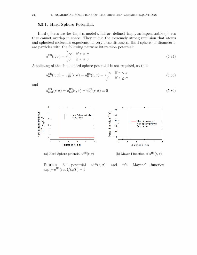
240 5. NUMERICAL SOLUTIONS OF THE ORNSTEIN ZERNIKE EQUATIONS
5.5.1. Hard Sphere Potential.
Hard spheres are the simplest model which are defined simply as impenetrable spheresthat cannot overlap in space. They mimic the extremely strong repulsion that atomsand spherical molecules experience at very close distances. Hard spheres of diameter σare particles with the following pairwise interaction potential:
uHS(r, σ) =
∞ if r < σ
0 if r ≥ σ(5.84)
A splitting of the simple hard sphere potential is not required, so that
uHSref (r, σ) = uHS
SR(r, σ) = uHSR (r, σ) =
∞ if r < σ
0 if r ≥ σ(5.85)
and
uHSpert(r, σ) = uHS
LR(r, σ) = uHSA (r, σ) ≡ 0 (5.86)
(a) Hard Sphere potential uHS(r, σ) (b) Mayer-f function of uHS(r, σ)
Figure 5.1. potential uHS(r, σ) and it’s Mayer-f functionexp(−uHS(r, σ)/kBT )− 1
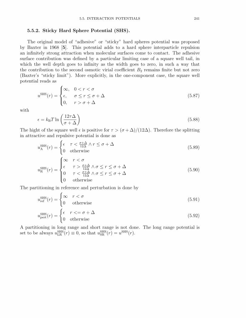
5.5. INTERACTION POTENTIALS 241
5.5.2. Sticky Hard Sphere Potential (SHS).
The original model of “adhesive” or “sticky” hard spheres potential was proposedby Baxter in 1968 [5]. This potential adds to a hard sphere interparticle repulsionan infinitely strong attraction when molecular surfaces come to contact. The adhesivesurface contribution was defined by a particular limiting case of a square well tail, inwhich the well depth goes to infinity as the width goes to zero, in such a way thatthe contribution to the second osmotic virial coefficient B2 remains finite but not zero(Baxter’s “sticky limit”). More explicitly, in the one-component case, the square wellpotential reads as
uSHS(r) =
∞, 0 < r < σ
ε, σ ≤ r ≤ σ + ∆
0, r > σ + ∆
(5.87)
with
ε = kBT ln
(12τ∆
σ + ∆
)(5.88)
The hight of the square well ε is positive for τ > (σ+ ∆)/(12∆). Therefore the splittingin attractive and repulsive potential is done as
uSHSA (r) =
ε τ < σ+∆
12∆∧ r ≤ σ + ∆
0 otherwise(5.89)
uSHSR (r) =
∞ r < σ
ε τ > σ+∆12∆∧ σ ≤ r ≤ σ + ∆
0 τ < σ+∆12∆∧ σ ≤ r ≤ σ + ∆
0 otherwise
(5.90)
The partitioning in reference and perturbation is done by
uSHSref (r) =
∞ r < σ
0 otherwise(5.91)
uSHSpert(r) =
ε r <= σ + ∆
0 otherwise(5.92)
A partitioning in long range and short range is not done. The long range potential isset to be always uSHS
LR (r) ≡ 0, so that uSHSSR (r) = uSHS(r).
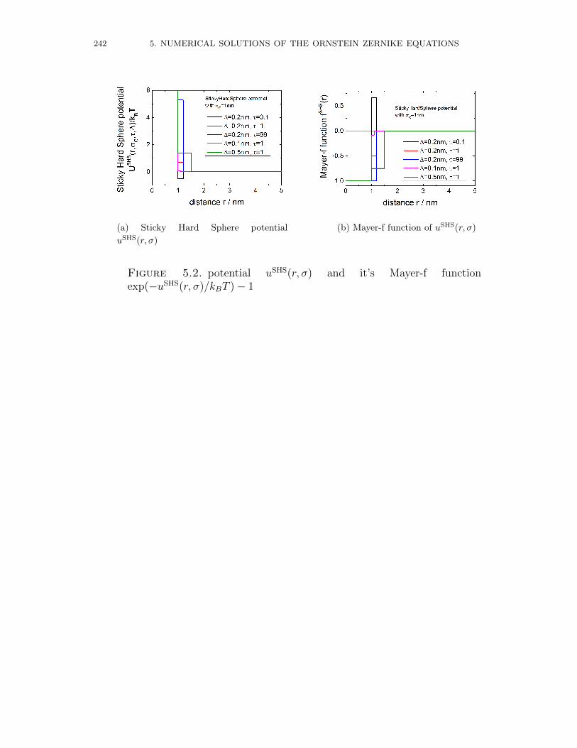
242 5. NUMERICAL SOLUTIONS OF THE ORNSTEIN ZERNIKE EQUATIONS
(a) Sticky Hard Sphere potential
uSHS(r, σ)
(b) Mayer-f function of uSHS(r, σ)
Figure 5.2. potential uSHS(r, σ) and it’s Mayer-f functionexp(−uSHS(r, σ)/kBT )− 1
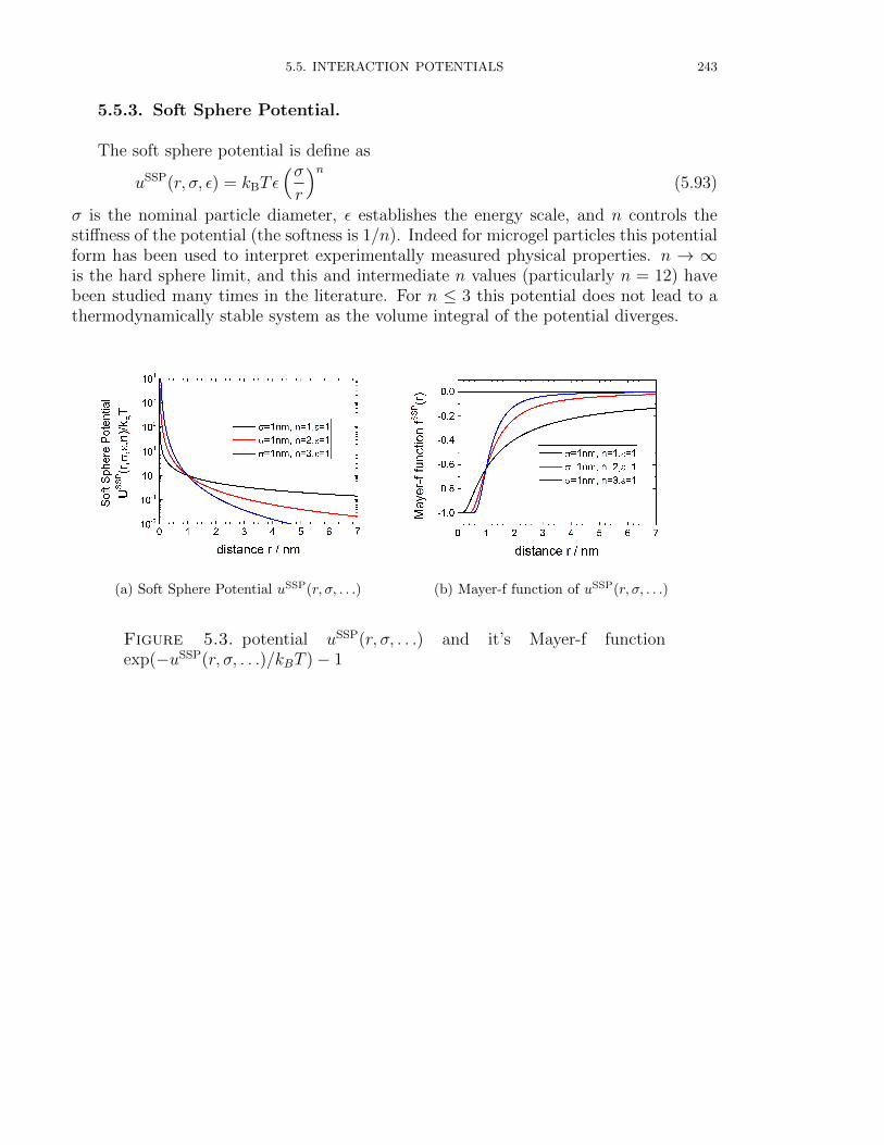
5.5. INTERACTION POTENTIALS 243
5.5.3. Soft Sphere Potential.
The soft sphere potential is define as
uSSP(r, σ, ε) = kBTε(σr
)n(5.93)
σ is the nominal particle diameter, ε establishes the energy scale, and n controls thestiffness of the potential (the softness is 1/n). Indeed for microgel particles this potentialform has been used to interpret experimentally measured physical properties. n → ∞is the hard sphere limit, and this and intermediate n values (particularly n = 12) havebeen studied many times in the literature. For n ≤ 3 this potential does not lead to athermodynamically stable system as the volume integral of the potential diverges.
(a) Soft Sphere Potential uSSP(r, σ, . . .) (b) Mayer-f function of uSSP(r, σ, . . .)
Figure 5.3. potential uSSP(r, σ, . . .) and it’s Mayer-f functionexp(−uSSP(r, σ, . . .)/kBT )− 1

244 5. NUMERICAL SOLUTIONS OF THE ORNSTEIN ZERNIKE EQUATIONS
5.5.4. Penetrable Sphere Model.
The penetrable sphere model was used by Marquest and Witten [90] who suggestedit as a prototype for the interaction between micelles in a solvent. The potential isdefined as [90, 142]
uPSM(r, σ, ε) =
kBTε for r ≤ σ
0 for r > σ(5.94)
(a) Potential of the Penetrable Sphere
Model (PSM) uPSM(r, σ, . . .)
(b) Mayer-f function of uPSM(r, σ, . . .)
Figure 5.4. potential uPSM(r, σ, . . .) and it’s Mayer-f functionexp(−uPSM(r, σ, . . .)/kBT )− 1
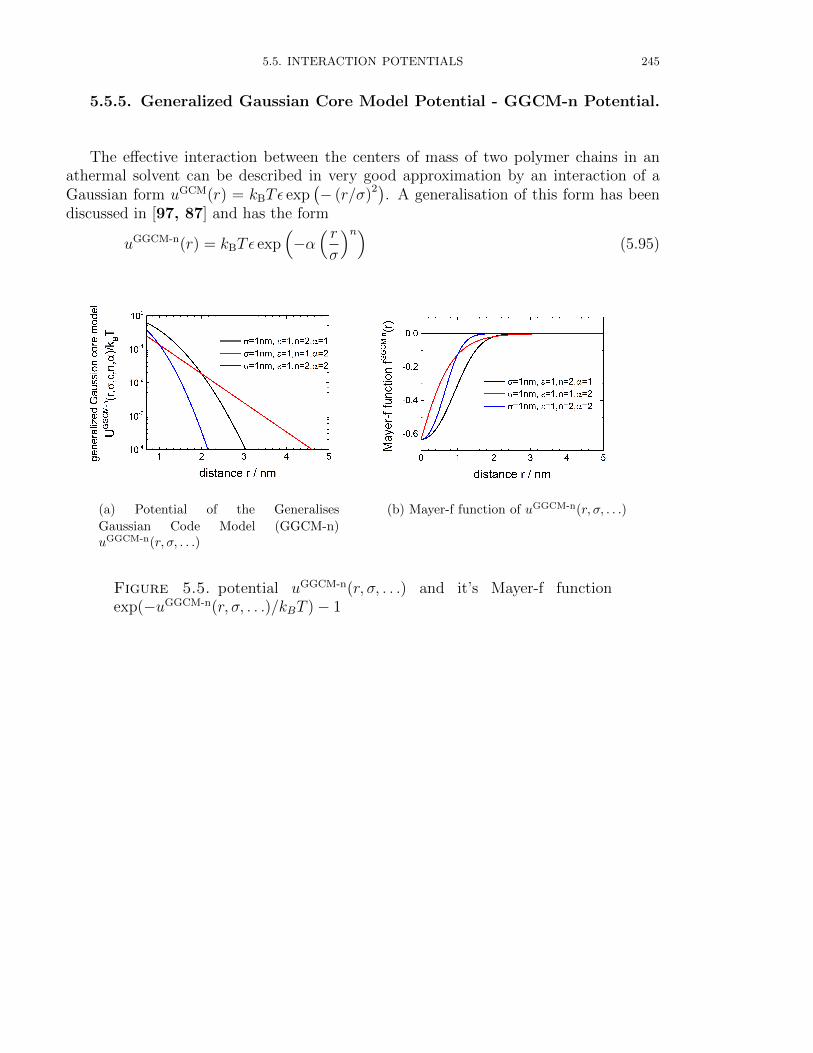
5.5. INTERACTION POTENTIALS 245
5.5.5. Generalized Gaussian Core Model Potential - GGCM-n Potential.
The effective interaction between the centers of mass of two polymer chains in anathermal solvent can be described in very good approximation by an interaction of aGaussian form uGCM(r) = kBTε exp
(− (r/σ)2). A generalisation of this form has been
discussed in [97, 87] and has the form
uGGCM-n(r) = kBTε exp(−α( rσ
)n)(5.95)
(a) Potential of the Generalises
Gaussian Code Model (GGCM-n)uGGCM-n(r, σ, . . .)
(b) Mayer-f function of uGGCM-n(r, σ, . . .)
Figure 5.5. potential uGGCM-n(r, σ, . . .) and it’s Mayer-f functionexp(−uGGCM-n(r, σ, . . .)/kBT )− 1
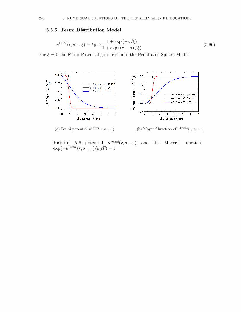
246 5. NUMERICAL SOLUTIONS OF THE ORNSTEIN ZERNIKE EQUATIONS
5.5.6. Fermi Distribution Model.
uFDM(r, σ, ε, ξ) = kBTε1 + exp (−σ/ξ)
1 + exp ((r − σ) /ξ)(5.96)
For ξ = 0 the Fermi Potential goes over into the Penetrable Sphere Model.
(a) Fermi potential uFermi(r, σ, . . .) (b) Mayer-f function of uFermi(r, σ, . . .)
Figure 5.6. potential uFermi(r, σ, . . .) and it’s Mayer-f functionexp(−uFermi(r, σ, . . .)/kBT )− 1
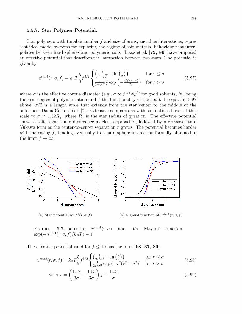
5.5. INTERACTION POTENTIALS 247
5.5.7. Star Polymer Potential.
Star polymers with tunable number f and size of arms, and thus interactions, repre-sent ideal model systems for exploring the regime of soft material behaviour that inter-polates between hard spheres and polymeric coils. Likos et al. [79, 80] have proposedan effective potential that describes the interaction between two stars. The potential isgiven by
ustar1(r, σ, f) = kBT5
8f 3/2
(
11+√f− ln
(rσ
))for r ≤ σ
11+√fσr
exp(−√f (r−σ)
2σ
)for r > σ
(5.97)
where σ is the effective corona diameter (e.g., σ ∝ f 1/5N3/5a for good solvents, Na being
the arm degree of polymerization and f the functionality of the star). In equation 5.97above, σ/2 is a length scale that extends from the star center to the middle of theoutermost DaoudCotton blob [?]. Extensive comparisons with simulations have set thisscale to σ ∼= 1.32Rg, where Rg is the star radius of gyration. The effective potentialshows a soft, logarithmic divergence at close approaches, followed by a crossover to aYukawa form as the center-to-center separation r grows. The potential becomes harderwith increasing f , tending eventually to a hard-sphere interaction formally obtained inthe limit f →∞.
(a) Star potential ustar1(r, σ, f) (b) Mayer-f function of ustar1(r, σ, f)
Figure 5.7. potential ustar1(r, σ) and it’s Mayer-f functionexp(−ustar1(r, σ, f)/kBT )− 1
The effective potential valid for f ≤ 10 has the form [68, 37, 80]:
ustar2(r, σ, f) = kBT5
8f 3/2
(1
2τ2σ2 − ln(rσ
))for r ≤ σ
12τ2σ2 exp (−τ 2(r2 − σ2)) for r > σ
(5.98)
with τ =
(1.12
3σ− 1.03
3σ
)f +
1.03
σ(5.99)
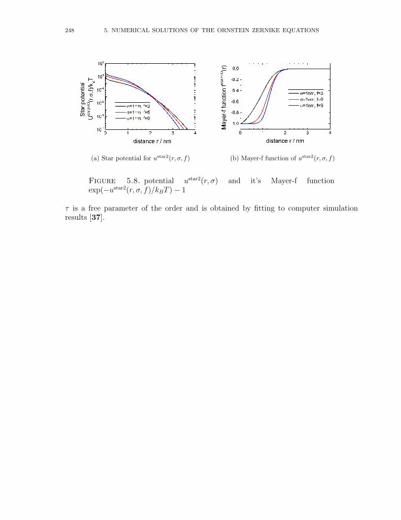
248 5. NUMERICAL SOLUTIONS OF THE ORNSTEIN ZERNIKE EQUATIONS
(a) Star potential for ustar2(r, σ, f) (b) Mayer-f function of ustar2(r, σ, f)
Figure 5.8. potential ustar2(r, σ) and it’s Mayer-f functionexp(−ustar2(r, σ, f)/kBT )− 1
τ is a free parameter of the order and is obtained by fitting to computer simulationresults [37].
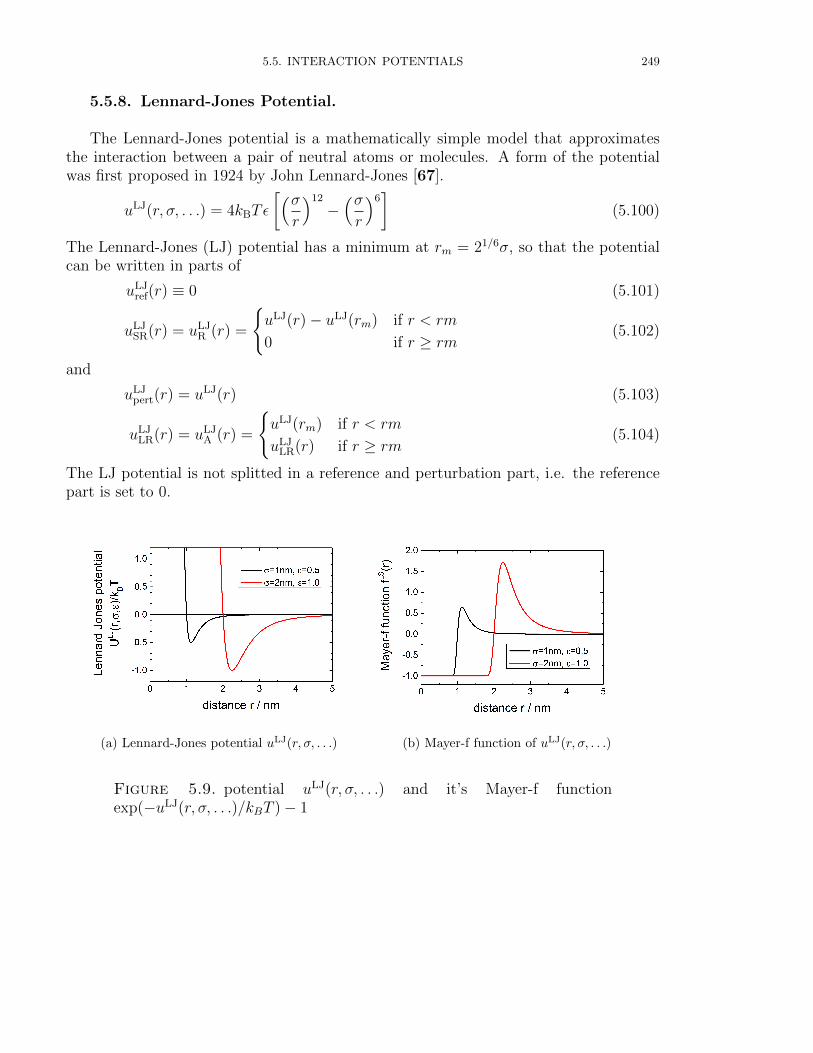
5.5. INTERACTION POTENTIALS 249
5.5.8. Lennard-Jones Potential.
The Lennard-Jones potential is a mathematically simple model that approximatesthe interaction between a pair of neutral atoms or molecules. A form of the potentialwas first proposed in 1924 by John Lennard-Jones [67].
uLJ(r, σ, . . .) = 4kBTε
[(σr
)12
−(σr
)6]
(5.100)
The Lennard-Jones (LJ) potential has a minimum at rm = 21/6σ, so that the potentialcan be written in parts of
uLJref(r) ≡ 0 (5.101)
uLJSR(r) = uLJ
R (r) =
uLJ(r)− uLJ(rm) if r < rm
0 if r ≥ rm(5.102)
and
uLJpert(r) = uLJ(r) (5.103)
uLJLR(r) = uLJ
A (r) =
uLJ(rm) if r < rm
uLJLR(r) if r ≥ rm
(5.104)
The LJ potential is not splitted in a reference and perturbation part, i.e. the referencepart is set to 0.
(a) Lennard-Jones potential uLJ(r, σ, . . .) (b) Mayer-f function of uLJ(r, σ, . . .)
Figure 5.9. potential uLJ(r, σ, . . .) and it’s Mayer-f functionexp(−uLJ(r, σ, . . .)/kBT )− 1
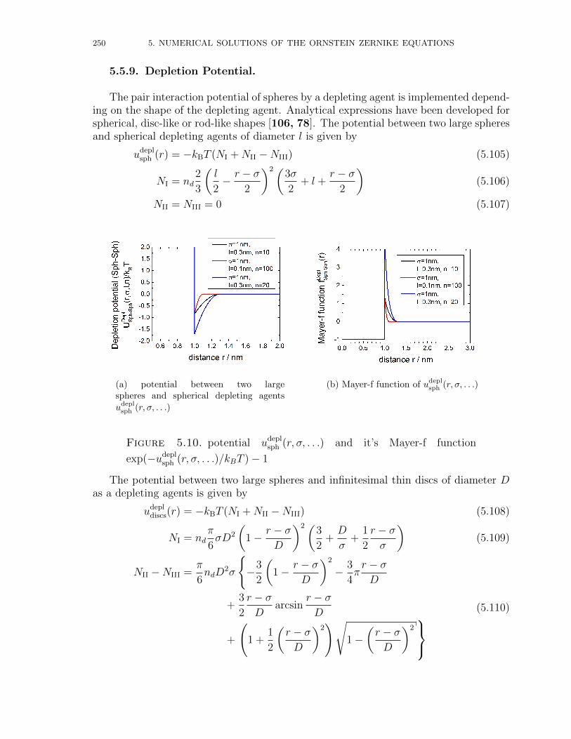
250 5. NUMERICAL SOLUTIONS OF THE ORNSTEIN ZERNIKE EQUATIONS
5.5.9. Depletion Potential.
The pair interaction potential of spheres by a depleting agent is implemented depend-ing on the shape of the depleting agent. Analytical expressions have been developed forspherical, disc-like or rod-like shapes [106, 78]. The potential between two large spheresand spherical depleting agents of diameter l is given by
udeplsph (r) = −kBT (NI +NII −NIII) (5.105)
NI = nd2
3
(l
2− r − σ
2
)2(3σ
2+ l +
r − σ2
)(5.106)
NII = NIII = 0 (5.107)
(a) potential between two largespheres and spherical depleting agents
udeplsph (r, σ, . . .)
(b) Mayer-f function of udeplsph (r, σ, . . .)
Figure 5.10. potential udeplsph (r, σ, . . .) and it’s Mayer-f function
exp(−udeplsph (r, σ, . . .)/kBT )− 1
The potential between two large spheres and infinitesimal thin discs of diameter Das a depleting agents is given by
udepldiscs(r) = −kBT (NI +NII −NIII) (5.108)
NI = ndπ
6σD2
(1− r − σ
D
)2(3
2+D
σ+
1
2
r − σσ
)(5.109)
NII −NIII =π
6ndD
2σ
−3
2
(1− r − σ
D
)2
− 3
4πr − σD
+3
2
r − σD
arcsinr − σD
+
(1 +
1
2
(r − σD
)2)√
1−(r − σD
)2
(5.110)
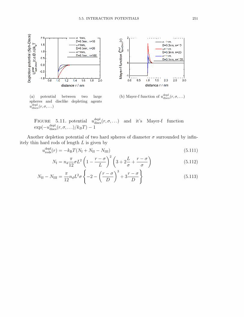
5.5. INTERACTION POTENTIALS 251
(a) potential between two largespheres and disclike depleting agents
udepldiscs(r, σ, . . .)
(b) Mayer-f function of udepldiscs(r, σ, . . .)
Figure 5.11. potential udepldiscs(r, σ, . . .) and it’s Mayer-f function
exp(−udepldiscs(r, σ, . . .)/kBT )− 1
Another depletion potential of two hard spheres of diameter σ surrounded by infin-itely thin hard rods of length L is given by
udeplrods(r) = −kBT (NI +NII −NIII) (5.111)
NI = ndπ
12σL2
(1− r − σ
L
)2(3 + 2
L
σ+r − σσ
)(5.112)
NII −NIII =π
12ndL
2σ
−2−
(r − σD
)3
+ 3r − σD
(5.113)

252 5. NUMERICAL SOLUTIONS OF THE ORNSTEIN ZERNIKE EQUATIONS
(a) potential between two large spheres
and rodlike depleting agents udeplrods(r, σ, . . .)
(b) Mayer-f function of udeplrods(r, σ, . . .)
Figure 5.12. potential udeplrods(r, σ, . . .) and it’s Mayer-f function
exp(−udeplrods(r, σ, . . .)/kBT )− 1
5.5.10. Ionic Microgel Potential.
According to [81] the effective potential in ionic microgels can be partitioned in acontribution Φr≤σ(r) for the overlap region r ≤ σ and one Φr>σ(r) for r > σ.
uim(r) = kBT
Φr≤σ(r) for r ≤ σ
Φr>σ(r) for r > σ(5.114)
For the overlapping particle it has the form
Φr≤σ(r) =2Z2e2
εσ
[6
5− 2
( rσ
)2
+3
2
( rσ
)3
− 1
5
( rσ
)5]− 72Z2e2
εκ4σ4rΦind(r) (5.115)
where Φind(r) is given by the expression
Φind(r) =
(1− e−κr +
1
2κ2r2 +
1
24κ4r4
)(1− 4
κ2σ2
)+
4
κσe−κσ sinh (κr)
+
[e−κσ sinh (κσ) + κ2σr +
1
6κ4(σ3r + r3σ
)](1 +
4
κ2σ2
)− 4r
σ
(1 +
1
2κ2σ2 +
1
30κ4σ4
)− 8r3
3σ3
(κ2σ2
4+κ4σ4
12
)− 1
180
κ4
σ2r6
(5.116)
5.5. INTERACTION POTENTIALS 253
For the nonoverlapping distances the effective potential becomes
Φr>σ(r) =144Z2e2
εκ4σ4
[cosh (κσ/2)− 2 sinh (κσ/2)
κσ
]2e−κr
r(5.117)
254 5. NUMERICAL SOLUTIONS OF THE ORNSTEIN ZERNIKE EQUATIONS
5.5.11. DLVO Potential.
For the past half century or so, the stability of charged colloidal systems has gener-ally been described in terms of the DLVO (Derjaguin-Landau-Verwey-Overbeek) poten-tial between two colloidal particles. The DLVO potential is composed of a long-rangescreened Coulomb repulsion part uel(r) and a short-range van der Waals attraction partuvdW(r) [101].
uDLVO(r) =
∞ if r ≤ σ
uvdW(r) + uel(r) if r > σ(5.118)
with
uvdW(r) = −kBTAH
12
(σ2
(r2 − σ2)+(σr
)2
+ 2 ln
(1−
(σr
)2))
(5.119)
uel(r) = kBTLBZ2eff
1
(1 + κσ/2)2
exp (−κ(r − σ))
r(5.120)
AH is the Hamaker constant. LB = e2
4πεrε0kBTis the so-called Bjerrum length1. The
vacuum permittivity is ε0 = 8.854187817× 10⁻¹²[
Fm
]and the elementary electric charge
e = 1.602176565(35) × 10−19coulombs2. For water at 278 K with a relativ permittivityof εr = 78.7 the Bjerrum length is LB = 0.713nm. The effective macroion valency isdenoted Zeff, and κ−1 is the Debye-Huckel screening length due to all macroions. Thislength characterize the typical distance at which the charge at the origin is screened bythe other charges. It is given by κ2 = 4πLB
∑Ni=1 niZi, where ni is the number density
of ion i, Zi is the charge number of that ion, and the sum is taken over all ions in thesolution. A discussion about effective parameters can be found in [1, 137].
1In Gaussian units, 4πε0 = 1 and the Bjerrum length has the simpler form LB = e2
εrkBT.
2The Gaussian units use the statcoulomb (statC) instead. The conversion between C and statC isdifferent in different contexts. In case of electric charges 1C = 2997924580 statC ≈ 3.00× 10⁹ statC.
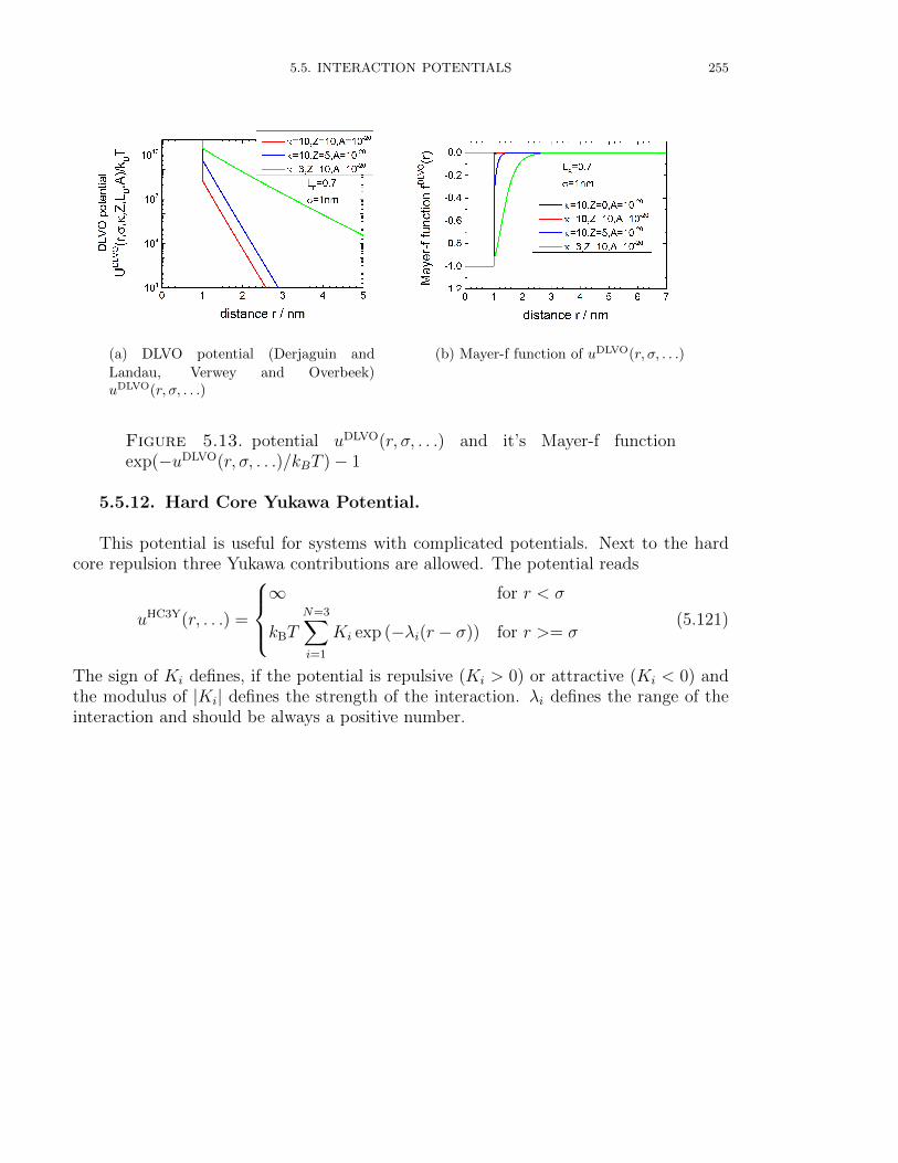
5.5. INTERACTION POTENTIALS 255
(a) DLVO potential (Derjaguin and
Landau, Verwey and Overbeek)uDLVO(r, σ, . . .)
(b) Mayer-f function of uDLVO(r, σ, . . .)
Figure 5.13. potential uDLVO(r, σ, . . .) and it’s Mayer-f functionexp(−uDLVO(r, σ, . . .)/kBT )− 1
5.5.12. Hard Core Yukawa Potential.
This potential is useful for systems with complicated potentials. Next to the hardcore repulsion three Yukawa contributions are allowed. The potential reads
uHC3Y(r, . . .) =
∞ for r < σ
kBTN=3∑i=1
Ki exp (−λi(r − σ)) for r >= σ(5.121)
The sign of Ki defines, if the potential is repulsive (Ki > 0) or attractive (Ki < 0) andthe modulus of |Ki| defines the strength of the interaction. λi defines the range of theinteraction and should be always a positive number.
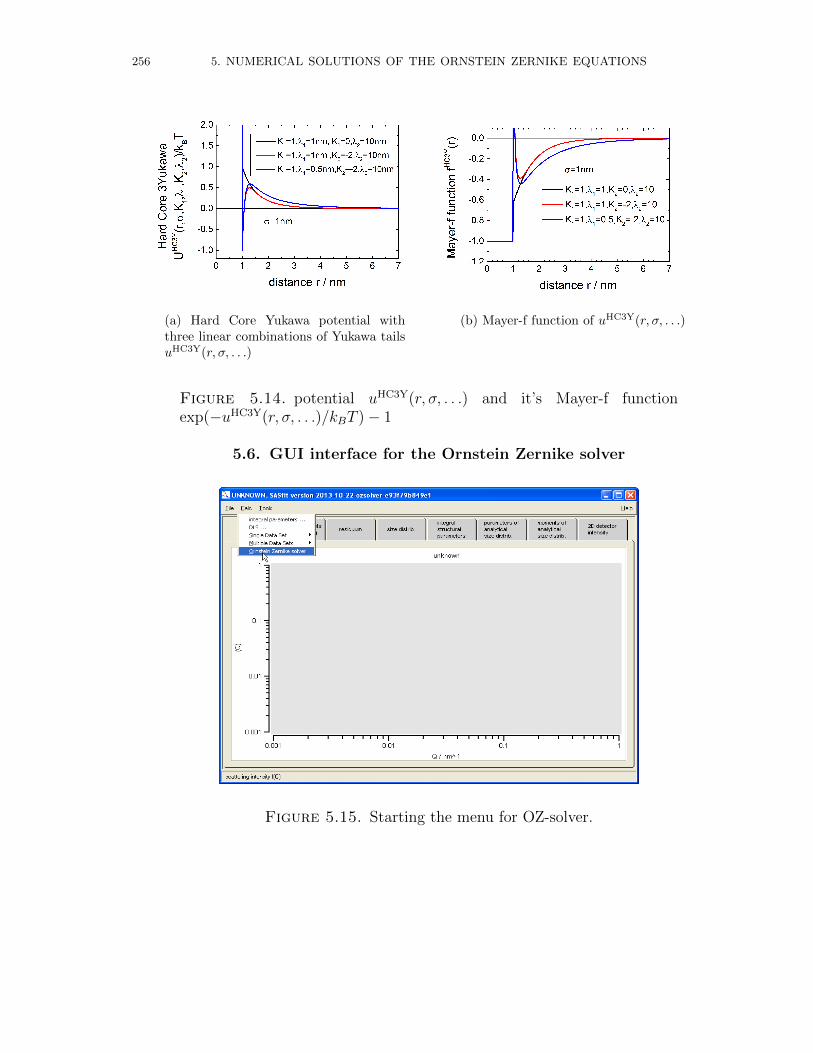
256 5. NUMERICAL SOLUTIONS OF THE ORNSTEIN ZERNIKE EQUATIONS
(a) Hard Core Yukawa potential withthree linear combinations of Yukawa tailsuHC3Y(r, σ, . . .)
(b) Mayer-f function of uHC3Y(r, σ, . . .)
Figure 5.14. potential uHC3Y(r, σ, . . .) and it’s Mayer-f functionexp(−uHC3Y(r, σ, . . .)/kBT )− 1
5.6. GUI interface for the Ornstein Zernike solver
Figure 5.15. Starting the menu for OZ-solver.
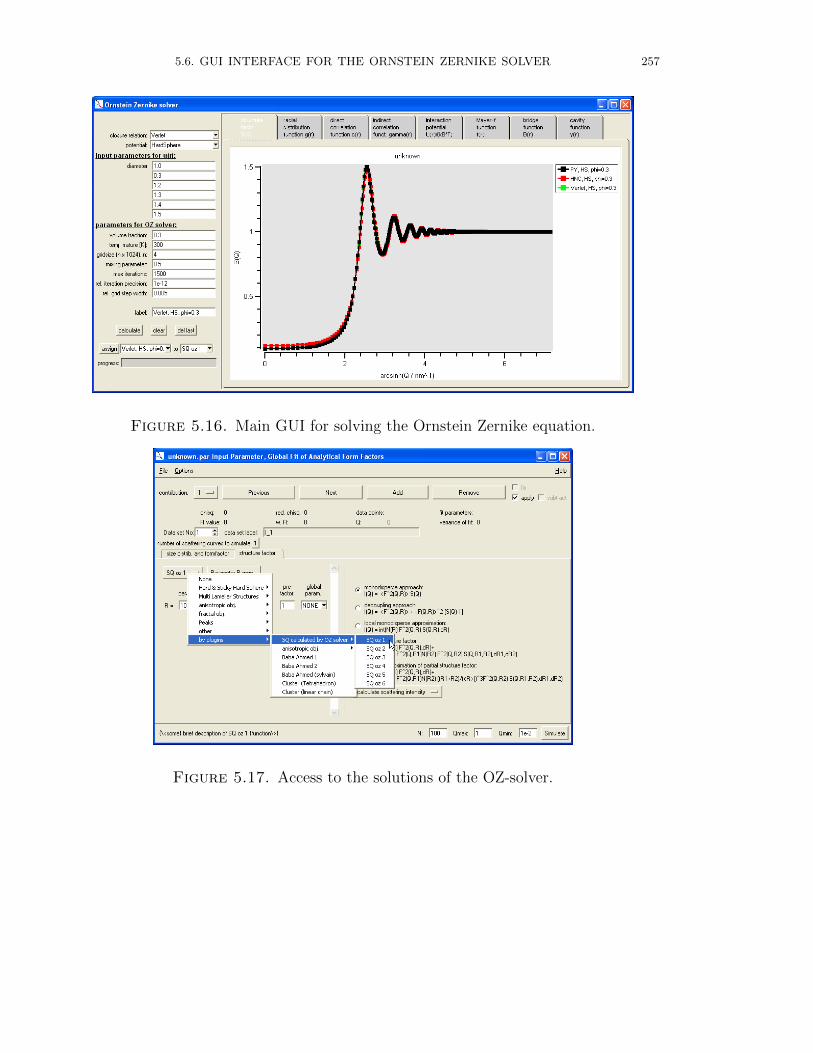
5.6. GUI INTERFACE FOR THE ORNSTEIN ZERNIKE SOLVER 257
Figure 5.16. Main GUI for solving the Ornstein Zernike equation.
Figure 5.17. Access to the solutions of the OZ-solver.

CHAPTER 6
Size Distributions
6.1. Delta
Choosing Delta as a size distribution simply scales the form factor with a constantvalue N
Input Parameters for size distribution Delta:
N: particle number density N
259
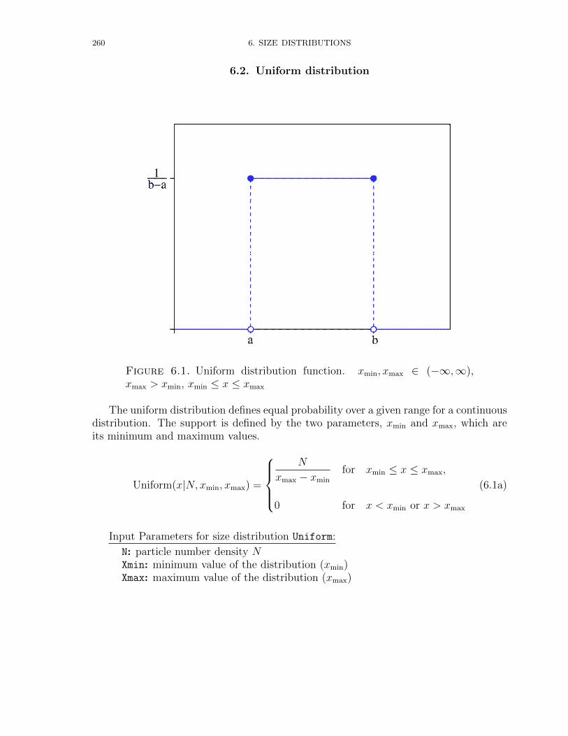
260 6. SIZE DISTRIBUTIONS
6.2. Uniform distribution
Figure 6.1. Uniform distribution function. xmin, xmax ∈ (−∞,∞),xmax > xmin, xmin ≤ x ≤ xmax
The uniform distribution defines equal probability over a given range for a continuousdistribution. The support is defined by the two parameters, xmin and xmax, which areits minimum and maximum values.
Uniform(x|N, xmin, xmax) =
N
xmax − xmin
for xmin ≤ x ≤ xmax,
0 for x < xmin or x > xmax
(6.1a)
Input Parameters for size distribution Uniform:
N: particle number density NXmin: minimum value of the distribution (xmin)Xmax: maximum value of the distribution (xmax)
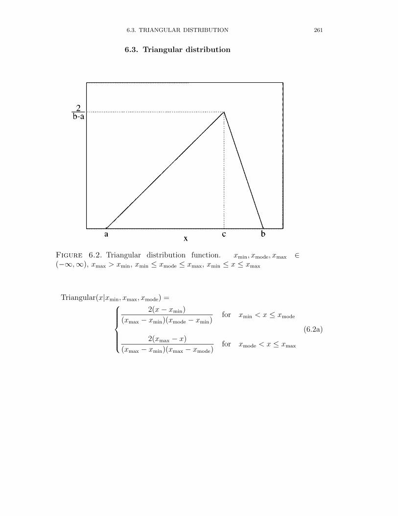
6.3. TRIANGULAR DISTRIBUTION 261
6.3. Triangular distribution
Figure 6.2. Triangular distribution function. xmin, xmode, xmax ∈(−∞,∞), xmax > xmin, xmin ≤ xmode ≤ xmax, xmin ≤ x ≤ xmax
Triangular(x|xmin, xmax, xmode) =2(x− xmin)
(xmax − xmin)(xmode − xmin)for xmin < x ≤ xmode
2(xmax − x)
(xmax − xmin)(xmax − xmode)for xmode < x ≤ xmax
(6.2a)
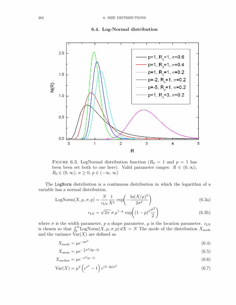
262 6. SIZE DISTRIBUTIONS
6.4. Log-Normal distribution
Figure 6.3. LogNormal distribution function (R0 = 1 and p = 1 hasbeen been set both to one here). Valid parameter ranges: R ∈ (0,∞),R0 ∈ (0,∞), σ ≥ 0, p ∈ (−∞,∞)
The LogNorm distribution is a continuous distribution in which the logarithm of avariable has a normal distribution.
LogNorm(X,µ, σ, p) =N
cLN
1
Xpexp
(− ln(X/µ)2
2σ2
)(6.3a)
cLN =√
2π σ µ1−p exp
((1− p)2σ
2
2
)(6.3b)
where σ is the width parameter, p a shape parameter, µ is the location parameter. cLN
is chosen so that∫∞
0LogNorm(X,µ, σ, p) dX = N The mode of the distribution Xmode
and the variance Var(X) are defined as
Xmode = µe−pσ2
(6.4)
Xmean = µe−12σ2(2p−3) (6.5)
Xmedian = µe−σ2(p−1) (6.6)
Var(X) = µ2(eσ
2 − 1)e(3−2p)σ2
(6.7)
6.4. LOG-NORMAL DISTRIBUTION 263
and the mth moment 〈Xm〉 of the LogNorm distribution as
〈Xm〉 =
∫Xm LogNorm(X) dX∫
LogNorm(X) dX= µm e
12σ2m(2−2p+m). (6.8)
The comulative distribution function is given by
FLogNorm = 1/2erf
[(p− 1)σ2 + ln(x/µ)√
2 σ
](6.9)
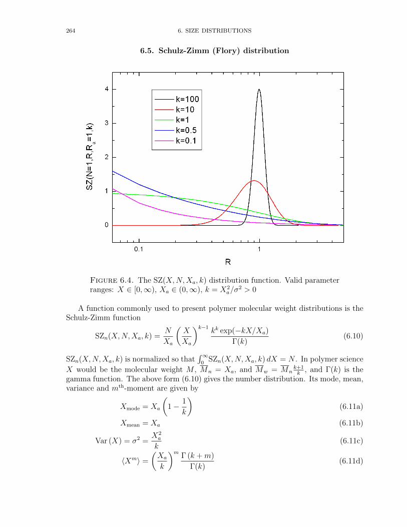
264 6. SIZE DISTRIBUTIONS
6.5. Schulz-Zimm (Flory) distribution
Figure 6.4. The SZ(X,N,Xa, k) distribution function. Valid parameterranges: X ∈ [0,∞), Xa ∈ (0,∞), k = X2
a/σ2 > 0
A function commonly used to present polymer molecular weight distributions is theSchulz-Zimm function
SZn(X,N,Xa, k) =N
Xa
(X
Xa
)k−1kk exp(−kX/Xa)
Γ(k)(6.10)
SZn(X,N,Xa, k) is normalized so that∫∞
0SZn(X,N,Xa, k) dX = N . In polymer science
X would be the molecular weight M , Mn = Xa, and Mw = Mnk+1k
, and Γ(k) is thegamma function. The above form (6.10) gives the number distribution. Its mode, mean,variance and mth-moment are given by
Xmode = Xa
(1− 1
k
)(6.11a)
Xmean = Xa (6.11b)
Var (X) = σ2 =X2a
k(6.11c)
〈Xm〉 =
(Xa
k
)mΓ (k +m)
Γ(k)(6.11d)
6.5. SCHULZ-ZIMM (FLORY) DISTRIBUTION 265
The corresponding weight distribution is
SZw(X,N,Xa, k) =X
Xa
SZn(X,N,Xa, k) =NXk
(kXa
)k+1
e−kXXa
Γ(k + 1)(6.12)
Also SZw(X,N,Xa, k) is normalized so that∫∞
0SZw(X,N,Xa, k) dX = N . The mode,
mean, variance and mth-moment of the weight distribution are given by
Xmode = Xa (6.13a)
Xmean = Xa1 + k
k(6.13b)
Var (X) = σ2 = X2a
1 + k
k2(6.13c)
〈Xm〉 =
(Xa
k
)mΓ (k +m+ 1)
Γ (k + 1)(6.13d)
266 6. SIZE DISTRIBUTIONS
6.6. Gamma distribution
The Gamma distribution is a two parameter continuous distribution with a scaleparameter θ and a shape parameter k.
gammaSD(x,N, xmode, σ) =N
θ
(xθ
)k−1 exp(−x/θ)Γ(k)
(6.14)
The mean xmean, mode xmode and variane σ2 of the distribution are given by
xmean = kθ (6.15)
xmode = (k − 1)θ for k ≥ 1 (6.16)
σ2 = kθ2 (6.17)
The gamma distribution is more flexible than the exponential or ξ2 distribution functionwhich are special cases of the gamma distribution function. When k is large, the gammadistribution closely approximates a normal distribution with the advantage that thegamma distribution has density only for positive real numbers. For small values of k thedistribution becomes a right tailed distribution.
The mth moment 〈Xm〉 of the size distribution is given by
〈Xm〉 = θmΓ(k +m)
Γ(k). (6.18)
In the present version the Gamma distribution is parametrised as a function of the modeand variance, i.e. with
k =xmode
√x2
mode + 4σ2 + x2mode + 2σ2
2σ2(6.19)
and
θ =1
2
(√x2
mode + 4σ2 − xmode
)(6.20)
gammaSD(R,N,Rm, σ) is normalized so that∫∞
0gammaSD(R,N,Rm, σ) dR = N .
Input Parameters for model Sphere:
N: Nmode: mod of the distribution (maximum, most probable size) xmode > 0sigma: width parameter σ > 0. The variance of the distribution is σ2.
Note:
• The parameters mode and sigma needs to be positive.

6.6. GAMMA DISTRIBUTION 267
Figure 6.5. The gammaSD(R,N, xmode, σ) distribution function. Validparameter ranges: x ∈ [0,∞), xmode ∈ (0,∞), σ > 0
268 6. SIZE DISTRIBUTIONS
6.7. PearsonIII distribution
The Pearson distribution is a family of probability distributions that are a general-isation of the normal distribution. The Pearson Type III distribution is given by theprobability density function
f(x) =1
β Γ(p)
(x− αβ
)p−1
e−(x−α)/β, (6.21)
where x ∈ [α,∞) and α, β and p are parameters of the distribution with β > 0 andp > 0 (Abramowitz and Stegun 1954, p. 930). Here, Γ() denotes the Gamma function.
• Mean:α + pβ
• Variance:pβ2
• Skewness:2√p
• Kurtosis:6
pThe Pearson Type III distribution is identical to the Gamma distribution (6.14). Whenα = 0, β = 2, and p is half-integer, the Pearson Type III distribution becomes the χ2
distribution of 2p degrees of freedom.
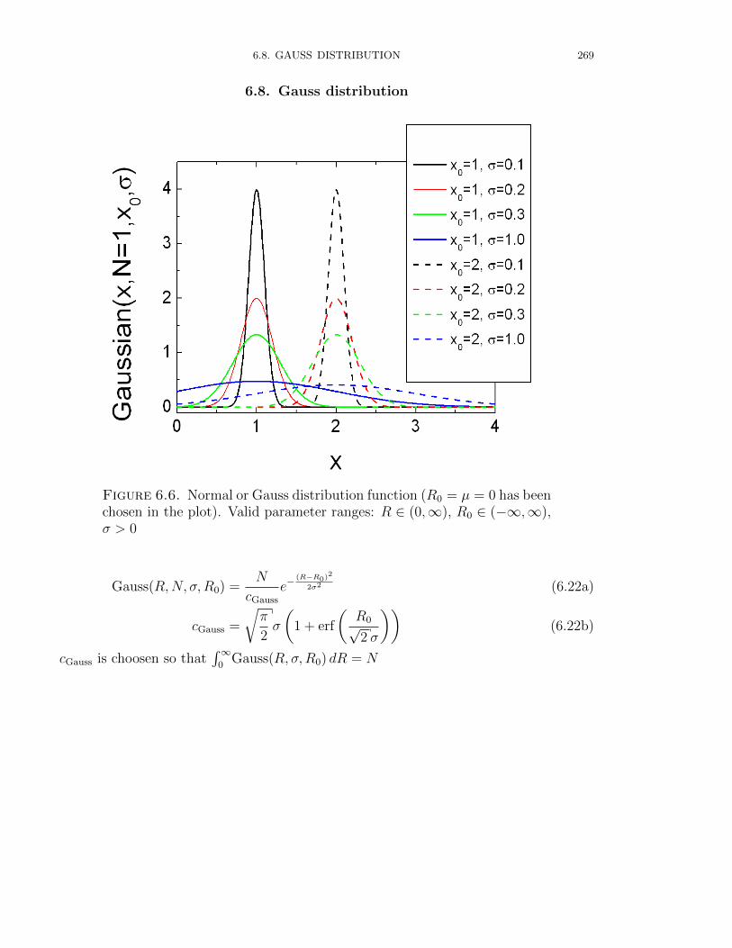
6.8. GAUSS DISTRIBUTION 269
6.8. Gauss distribution
Figure 6.6. Normal or Gauss distribution function (R0 = µ = 0 has beenchosen in the plot). Valid parameter ranges: R ∈ (0,∞), R0 ∈ (−∞,∞),σ > 0
Gauss(R,N, σ,R0) =N
cGauss
e−(R−R0)2
2σ2 (6.22a)
cGauss =
√π
2σ
(1 + erf
(R0√2 σ
))(6.22b)
cGauss is choosen so that∫∞
0Gauss(R, σ,R0) dR = N
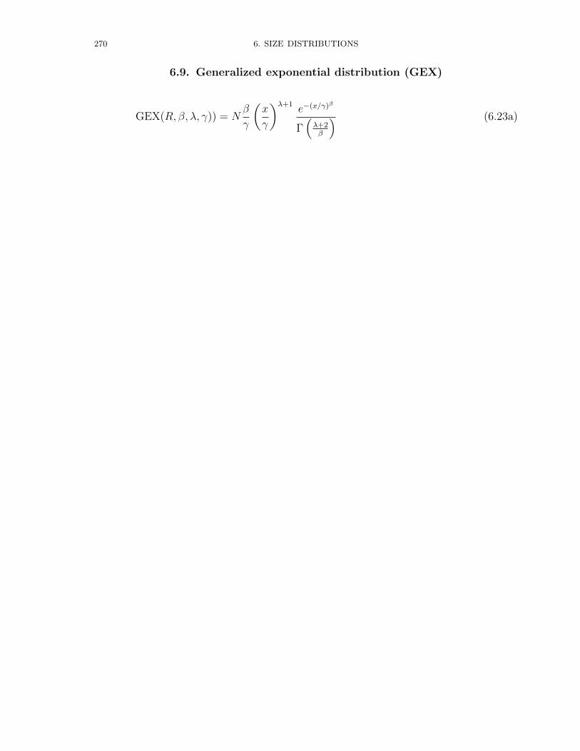
270 6. SIZE DISTRIBUTIONS
6.9. Generalized exponential distribution (GEX)
GEX(R, β, λ, γ)) = Nβ
γ
(x
γ
)λ+1e−(x/γ)β
Γ(λ+2β
) (6.23a)
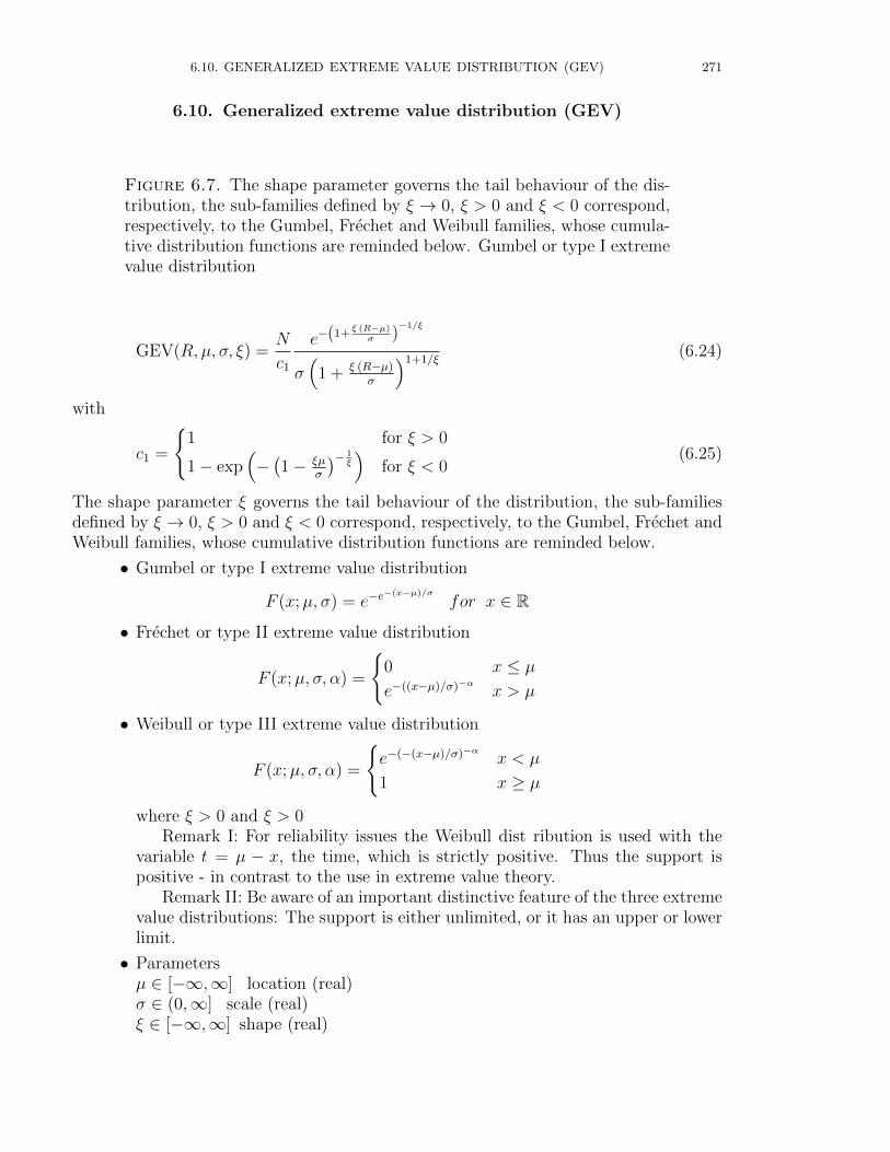
6.10. GENERALIZED EXTREME VALUE DISTRIBUTION (GEV) 271
6.10. Generalized extreme value distribution (GEV)
Figure 6.7. The shape parameter governs the tail behaviour of the dis-tribution, the sub-families defined by ξ → 0, ξ > 0 and ξ < 0 correspond,respectively, to the Gumbel, Frechet and Weibull families, whose cumula-tive distribution functions are reminded below. Gumbel or type I extremevalue distribution
GEV(R, µ, σ, ξ) =N
c1
e−(1+ξ (R−µ)
σ )−1/ξ
σ(
1 + ξ (R−µ)σ
)1+1/ξ(6.24)
with
c1 =
1 for ξ > 0
1− exp(−(1− ξµ
σ
)− 1ξ
)for ξ < 0
(6.25)
The shape parameter ξ governs the tail behaviour of the distribution, the sub-familiesdefined by ξ → 0, ξ > 0 and ξ < 0 correspond, respectively, to the Gumbel, Frechet andWeibull families, whose cumulative distribution functions are reminded below.
• Gumbel or type I extreme value distribution
F (x;µ, σ) = e−e−(x−µ)/σ
for x ∈ R
• Frechet or type II extreme value distribution
F (x;µ, σ, α) =
0 x ≤ µ
e−((x−µ)/σ)−α x > µ
• Weibull or type III extreme value distribution
F (x;µ, σ, α) =
e−(−(x−µ)/σ)−α x < µ
1 x ≥ µ
where ξ > 0 and ξ > 0Remark I: For reliability issues the Weibull dist ribution is used with the
variable t = µ − x, the time, which is strictly positive. Thus the support ispositive - in contrast to the use in extreme value theory.
Remark II: Be aware of an important distinctive feature of the three extremevalue distributions: The support is either unlimited, or it has an upper or lowerlimit.
• Parametersµ ∈ [−∞,∞] location (real)σ ∈ (0,∞] scale (real)ξ ∈ [−∞,∞] shape (real)
272 6. SIZE DISTRIBUTIONS
• Supportx > µ− σ/ξ (ξ > 0)x < µ− σ/ξ (ξ < 0)x ∈ [−∞,∞] (ξ = 0)
[1] http://en.wikipedia.org/wiki/Generalized_extreme_value_distribution
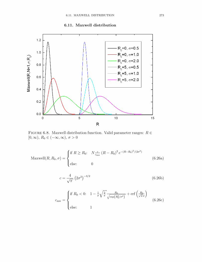
6.11. MAXWELL DISTRIBUTION 273
6.11. Maxwell distribution
Figure 6.8. Maxwell distribution function. Valid parameter ranges: R ∈[0,∞), R0 ∈ (−∞,∞), σ > 0
Maxwell(R,R0, σ) =
if R ≥ R0: N c
cmw(R−R0)2 e−(R−R0)2/(2σ2)
else: 0
(6.26a)
c =4√π
(2σ2)−3/2
(6.26b)
cmw =
if R0 < 0: 1− 1
σ
√2π
R0√exp(R2
0/σ2)
+ erf(
R0√2 σ
)else: 1
(6.26c)
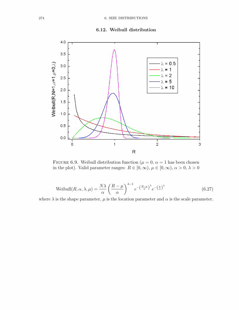
274 6. SIZE DISTRIBUTIONS
6.12. Weibull distribution
Figure 6.9. Weibull distribution function (µ = 0, α = 1 has been chosenin the plot). Valid parameter ranges: R ∈ [0,∞), µ ∈ [0,∞), α > 0, λ > 0
Weibull(R,α, λ, µ) =Nλ
α
(R− µα
)λ−1
e−(R−µα )λ
e−( µα)λ
(6.27)
where λ is the shape parameter, µ is the location parameter and α is the scale parameter.

6.13. FRACTAL SIZE DISTRIBUTION 275
6.13. fractal size distribution
Figure 6.10. fractal size distribution function. Valid parameter ranges:R ∈ [Rmin, Rmax], fD ∈ (−1,∞), Rmax > Rmin > 0
fractalSD(R,N,Rmin, Rmax, fD) =NfD
R−fDmin −R−fDmax
R−(1+fD) (6.28)


CHAPTER 7
Peak functions
277

278 7. PEAK FUNCTIONS
7.1. Beta
The Beta distribution is a very versatile function which can be used to modelseveral different shapes of probability density curves. In probability theory and statistics,the beta distribution is a family of continuous probability distributions defined on theinterval [0, 1] parameterized by two positive shape parameters, typically denoted by αand β.
pBeta(x;α, β) =
1
B(α,β)xα−1(1− x)β−1 for 0 < x < 1
0 otherwise(7.1)
The beta function, B, appears as a normalization constant to ensure that the totalprobability integrates to unity. α and β are positive numbers that define the shapeparameters. The mode of the beta distribution for shape parameters α > 1 and β > 1is given by
mode (pBeta) =α− 1
α + β − 2(7.2)
7.1.1. Beta (Amplitude).
yBeta(ampl) (x;A, xmin, xmax, α, β, c0) = ApBeta
(x−xmin
xmax−xmin;α, β
)pBeta
(α−1
α+β−2;α, β
) + c0 (7.3)
Required parameters:
ampl.: amplitude A of the Beta peakxmin: continuous lower boundary parameters xmin
xmax: continuous upper boundary parameters xmax
alpha: first shape parameter α > 1beta: second shape parameter β > 1backgr: offset c0
Note
• Both shape parameter needs to be larger than one (α, β > 1), as only than thedistribution has a peak shape.• where the Beta distribution is not defined the offset value is returned:∀x /∈ (xmin, xmax) yBeta(ampl)(x) = c0
• Default (size) distribution: Monodisperse
7.1.2. Beta (Area).
yBeta(area) (x;A, xmin, xmax, α, β, c0) = ApBeta
(x−xmin
xmax−xmin;α, β
)xmax − xmin
+ c0 (7.4)
Required parameters:
area: area A of the beta distribution
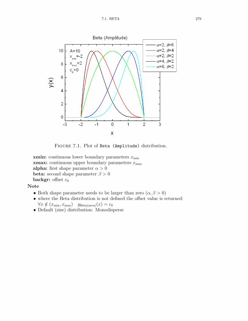
7.1. BETA 279
Figure 7.1. Plot of Beta (Amplitude) distribution.
xmin: continuous lower boundary parameters xmin
xmax: continuous upper boundary parameters xmax
alpha: first shape parameter α > 0beta: second shape parameter β > 0backgr: offset c0
Note
• Both shape parameter needs to be larger than zero (α, β > 0)• where the Beta distribution is not defined the offset value is returned:∀x /∈ (xmin, xmax) yBeta(area)(x) = c0
• Default (size) distribution: Monodisperse
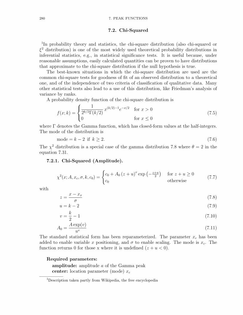
280 7. PEAK FUNCTIONS
7.2. Chi-Squared
1In probability theory and statistics, the chi-square distribution (also chi-squared orξ2 distribution) is one of the most widely used theoretical probability distributions ininferential statistics, e.g., in statistical significance tests. It is useful because, underreasonable assumptions, easily calculated quantities can be proven to have distributionsthat approximate to the chi-square distribution if the null hypothesis is true.
The best-known situations in which the chi-square distribution are used are thecommon chi-square tests for goodness of fit of an observed distribution to a theoreticalone, and of the independence of two criteria of classification of qualitative data. Manyother statistical tests also lead to a use of this distribution, like Friedman’s analysis ofvariance by ranks.
A probability density function of the chi-square distribution is
f(x; k) =
1
2k/2Γ(k/2)x(k/2)−1e−x/2 for x > 0
0 for x ≤ 0(7.5)
where Γ denotes the Gamma function, which has closed-form values at the half-integers.The mode of the distribution is
mode = k − 2 if k ≥ 2. (7.6)
The χ2 distribution is a special case of the gamma distribution 7.8 where θ = 2 in theequation 7.31.
7.2.1. Chi-Squared (Amplitude).
χ2(x;A, xc, σ, k, c0) =
c0 + A0 (z + u)v exp
(− z+u
2
)for z + u ≥ 0
c0 otherwise(7.7)
with
z =x− xxσ
(7.8)
u = k − 2 (7.9)
v =k
2− 1 (7.10)
A0 =A exp(v)
uv(7.11)
The standard statistical form has been reparameterized. The parameter xc has beenadded to enable variable x positioning, and σ to enable scaling. The mode is xc. Thefunction returns 0 for those x where it is undefined (z + u < 0).
Required parameters:
amplitude: amplitude a of the Gamma peakcenter: location parameter (mode) xc
1Description taken partly from Wikipedia, the free encyclopedia
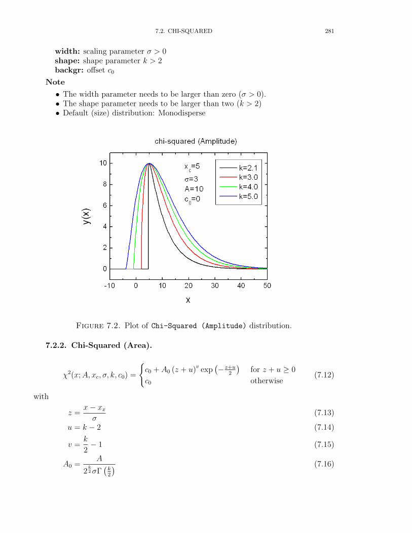
7.2. CHI-SQUARED 281
width: scaling parameter σ > 0shape: shape parameter k > 2backgr: offset c0
Note
• The width parameter needs to be larger than zero (σ > 0).• The shape parameter needs to be larger than two (k > 2)• Default (size) distribution: Monodisperse
Figure 7.2. Plot of Chi-Squared (Amplitude) distribution.
7.2.2. Chi-Squared (Area).
χ2(x;A, xc, σ, k, c0) =
c0 + A0 (z + u)v exp
(− z+u
2
)for z + u ≥ 0
c0 otherwise(7.12)
with
z =x− xxσ
(7.13)
u = k − 2 (7.14)
v =k
2− 1 (7.15)
A0 =A
2k2σΓ
(k2
) (7.16)
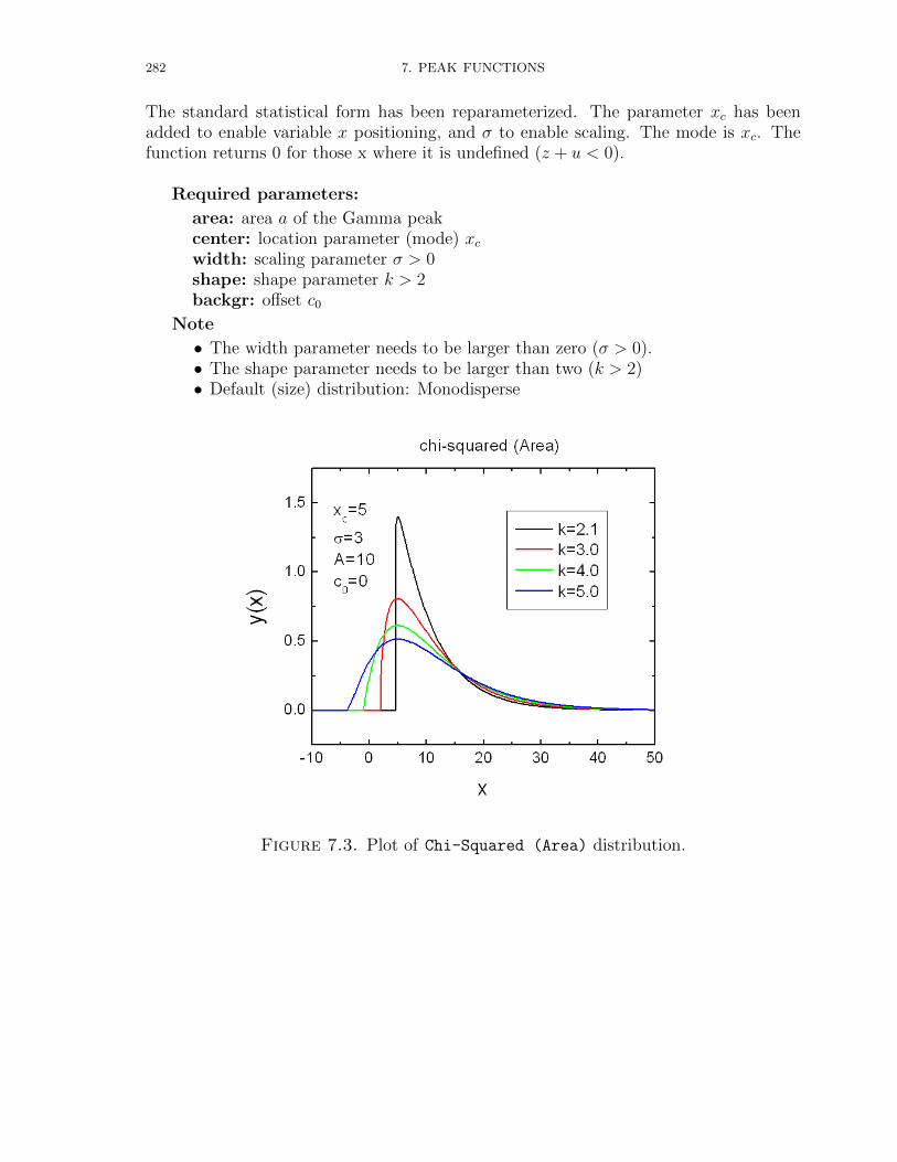
282 7. PEAK FUNCTIONS
The standard statistical form has been reparameterized. The parameter xc has beenadded to enable variable x positioning, and σ to enable scaling. The mode is xc. Thefunction returns 0 for those x where it is undefined (z + u < 0).
Required parameters:
area: area a of the Gamma peakcenter: location parameter (mode) xcwidth: scaling parameter σ > 0shape: shape parameter k > 2backgr: offset c0
Note
• The width parameter needs to be larger than zero (σ > 0).• The shape parameter needs to be larger than two (k > 2)• Default (size) distribution: Monodisperse
Figure 7.3. Plot of Chi-Squared (Area) distribution.

7.3. ERFC PEAK 283
7.3. Erfc peak
7.3.1. Erfc (Amplitude).
y(x; a, xc, σ, c0) = a erfc
((x− xcσ
)2)
+ c0 (7.17)
Required parameters:
ampl.: amplitude a of the erfc peakcenter: location parameter (mode) xcwidth: scaling parameter σ > 0backgr: offset c0
Note
• The width parameter needs to be non-zero (σ 6= 0).• Default (size) distribution: Monodisperse
Figure 7.4. Plot of Erfc (Amplitude) distribution.

284 7. PEAK FUNCTIONS
7.3.2. Erfc (Area).
y(x; a, xc, σ, c0) = aerfc
((x−xcσ
)2)
∫∞−∞ erfc
((x−xcσ
)2)dx
+ c0 (7.18)
Required parameters:
area: area a below the erfc peakcenter: location parameter (mode) xcwidth: scaling parameter σ > 0backgr: offset c0
Note
• The width parameter needs to be non-zero (σ 6= 0).• Default (size) distribution: Monodisperse
Figure 7.5. Plot of Erfc (Area) distribution.
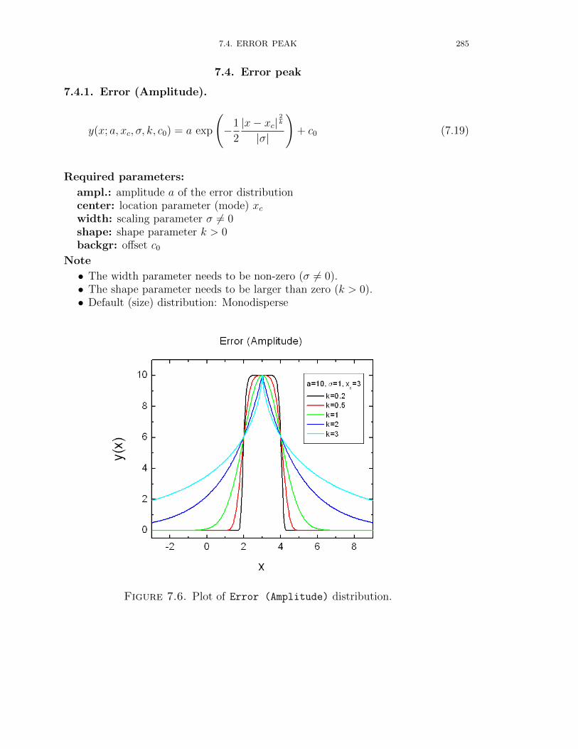
7.4. ERROR PEAK 285
7.4. Error peak
7.4.1. Error (Amplitude).
y(x; a, xc, σ, k, c0) = a exp
(−1
2
|x− xc|2k
|σ|
)+ c0 (7.19)
Required parameters:
ampl.: amplitude a of the error distributioncenter: location parameter (mode) xcwidth: scaling parameter σ 6= 0shape: shape parameter k > 0backgr: offset c0
Note
• The width parameter needs to be non-zero (σ 6= 0).• The shape parameter needs to be larger than zero (k > 0).• Default (size) distribution: Monodisperse
Figure 7.6. Plot of Error (Amplitude) distribution.
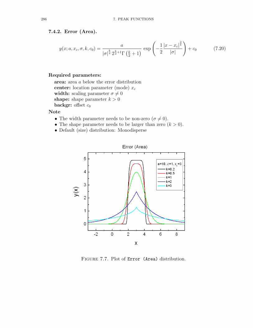
286 7. PEAK FUNCTIONS
7.4.2. Error (Area).
y(x; a, xc, σ, k, c0) =a
|σ|k2 2
k2
+1Γ(k2
+ 1) exp
(−1
2
|x− xc|2k
|σ|
)+ c0 (7.20)
Required parameters:
area: area a below the error distributioncenter: location parameter (mode) xcwidth: scaling parameter σ 6= 0shape: shape parameter k > 0backgr: offset c0
Note
• The width parameter needs to be non-zero (σ 6= 0).• The shape parameter needs to be larger than zero (k > 0).• Default (size) distribution: Monodisperse
Figure 7.7. Plot of Error (Area) distribution.
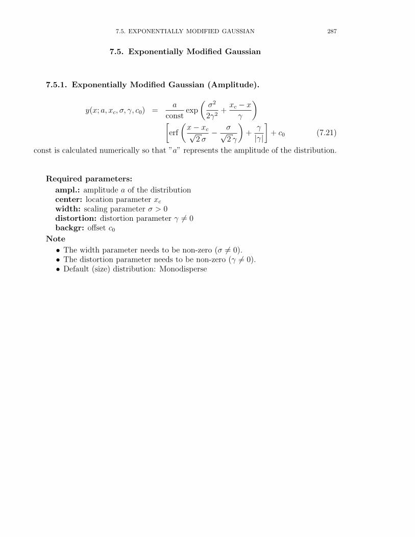
7.5. EXPONENTIALLY MODIFIED GAUSSIAN 287
7.5. Exponentially Modified Gaussian
7.5.1. Exponentially Modified Gaussian (Amplitude).
y(x; a, xc, σ, γ, c0) =a
constexp
(σ2
2γ2+xc − xγ
)[erf
(x− xc√
2 σ− σ√
2 γ
)+
γ
|γ|
]+ c0 (7.21)
const is calculated numerically so that ”a” represents the amplitude of the distribution.
Required parameters:
ampl.: amplitude a of the distributioncenter: location parameter xcwidth: scaling parameter σ > 0distortion: distortion parameter γ 6= 0backgr: offset c0
Note
• The width parameter needs to be non-zero (σ 6= 0).• The distortion parameter needs to be non-zero (γ 6= 0).• Default (size) distribution: Monodisperse

288 7. PEAK FUNCTIONS
Figure 7.8. Plot of Exponentially Modified Gaussian (Amplitude) distribution.
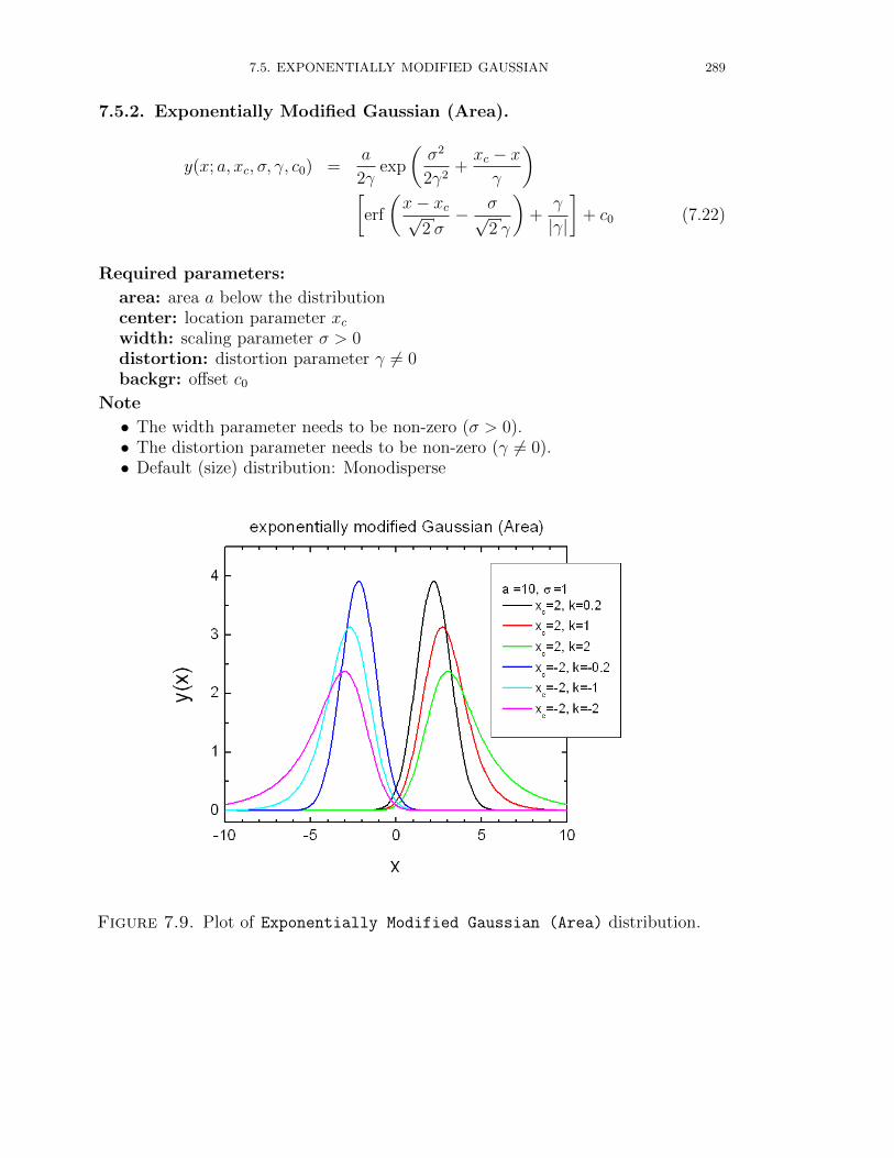
7.5. EXPONENTIALLY MODIFIED GAUSSIAN 289
7.5.2. Exponentially Modified Gaussian (Area).
y(x; a, xc, σ, γ, c0) =a
2γexp
(σ2
2γ2+xc − xγ
)[erf
(x− xc√
2 σ− σ√
2 γ
)+
γ
|γ|
]+ c0 (7.22)
Required parameters:
area: area a below the distributioncenter: location parameter xcwidth: scaling parameter σ > 0distortion: distortion parameter γ 6= 0backgr: offset c0
Note
• The width parameter needs to be non-zero (σ > 0).• The distortion parameter needs to be non-zero (γ 6= 0).• Default (size) distribution: Monodisperse
Figure 7.9. Plot of Exponentially Modified Gaussian (Area) distribution.
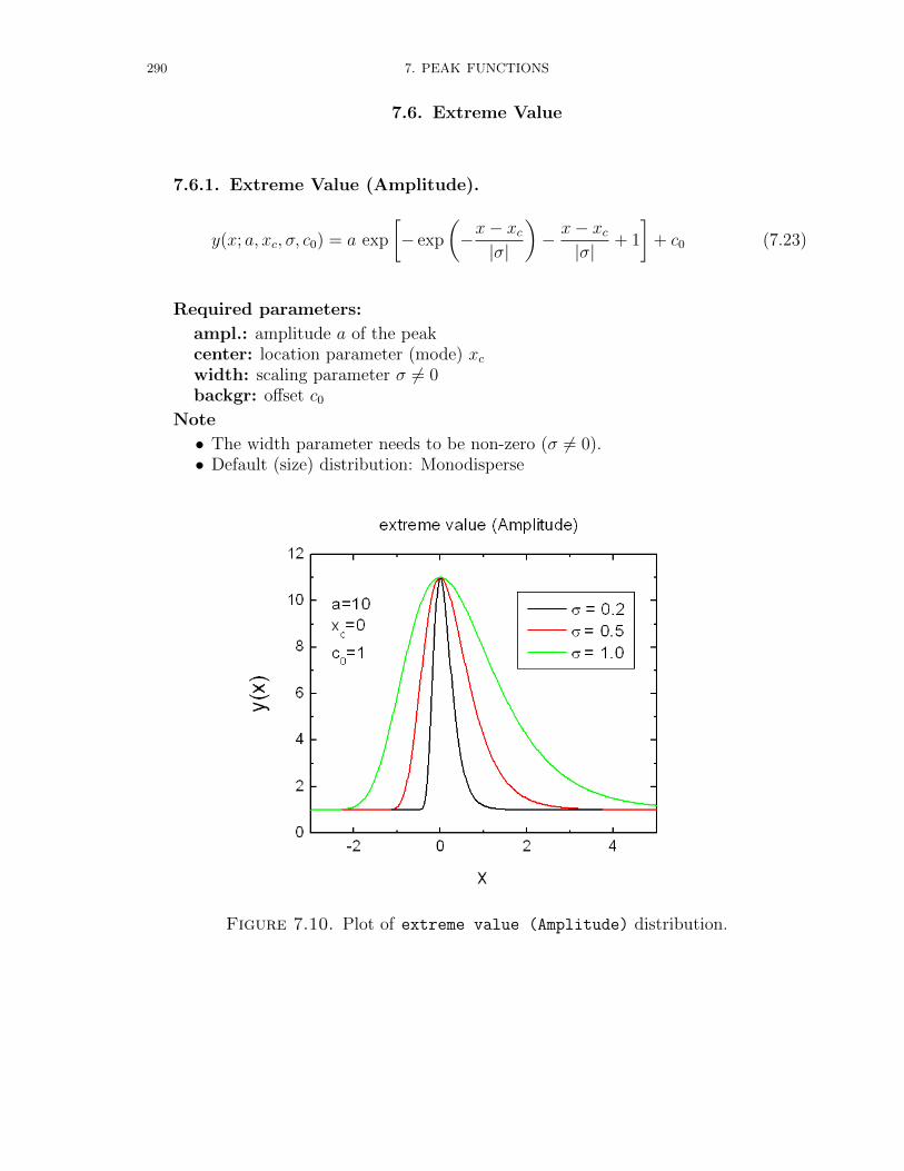
290 7. PEAK FUNCTIONS
7.6. Extreme Value
7.6.1. Extreme Value (Amplitude).
y(x; a, xc, σ, c0) = a exp
[− exp
(−x− xc|σ|
)− x− xc|σ|
+ 1
]+ c0 (7.23)
Required parameters:
ampl.: amplitude a of the peakcenter: location parameter (mode) xcwidth: scaling parameter σ 6= 0backgr: offset c0
Note
• The width parameter needs to be non-zero (σ 6= 0).• Default (size) distribution: Monodisperse
Figure 7.10. Plot of extreme value (Amplitude) distribution.
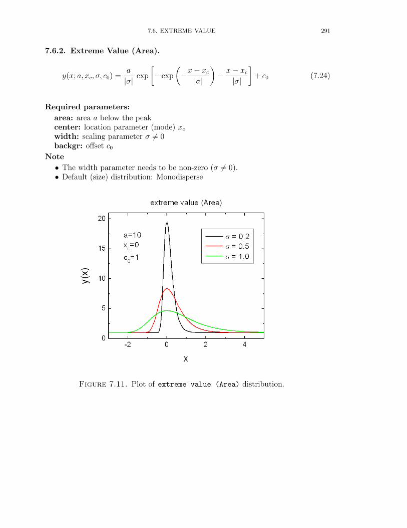
7.6. EXTREME VALUE 291
7.6.2. Extreme Value (Area).
y(x; a, xc, σ, c0) =a
|σ|exp
[− exp
(−x− xc|σ|
)− x− xc|σ|
]+ c0 (7.24)
Required parameters:
area: area a below the peakcenter: location parameter (mode) xcwidth: scaling parameter σ 6= 0backgr: offset c0
Note
• The width parameter needs to be non-zero (σ 6= 0).• Default (size) distribution: Monodisperse
Figure 7.11. Plot of extreme value (Area) distribution.
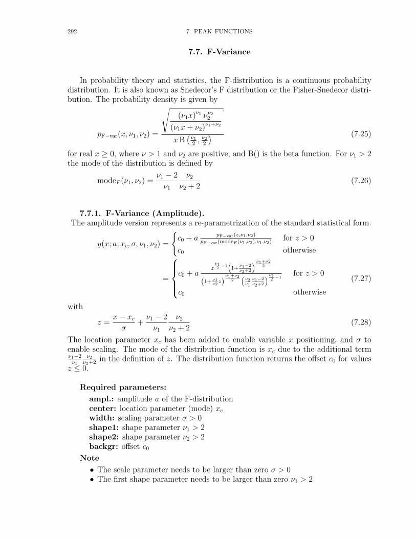
292 7. PEAK FUNCTIONS
7.7. F-Variance
In probability theory and statistics, the F-distribution is a continuous probabilitydistribution. It is also known as Snedecor’s F distribution or the Fisher-Snedecor distri-bution. The probability density is given by
pF−var(x, ν1, ν2) =
√(ν1x)ν1 νν2
2
(ν1x+ ν2)ν1+ν2
xB(ν1
2, ν2
2
) (7.25)
for real x ≥ 0, where ν > 1 and ν2 are positive, and B() is the beta function. For ν1 > 2the mode of the distribution is defined by
modeF (ν1, ν2) =ν1 − 2
ν1
ν2
ν2 + 2(7.26)
7.7.1. F-Variance (Amplitude).The amplitude version represents a re-parametrization of the standard statistical form.
y(x; a, xc, σ, ν1, ν2) =
c0 + a pF−var(z,ν1,ν2)
pF−var(modeF (ν1,ν2),ν1,ν2)for z > 0
c0 otherwise
=
c0 + a
zν12 −1
(1+
ν1−2ν2+2
) ν1+ν22
(1+ ν1ν2z)
ν1+ν22
(ν2ν1
ν1−2ν2+2
) ν12 −1
for z > 0
c0 otherwise
(7.27)
with
z =x− xcσ
+ν1 − 2
ν1
ν2
ν2 + 2(7.28)
The location parameter xc has been added to enable variable x positioning, and σ toenable scaling. The mode of the distribution function is xc due to the additional termν1−2ν1
ν2
ν2+2in the definition of z. The distribution function returns the offset c0 for values
z ≤ 0.
Required parameters:
ampl.: amplitude a of the F-distributioncenter: location parameter (mode) xcwidth: scaling parameter σ > 0shape1: shape parameter ν1 > 2shape2: shape parameter ν2 > 2backgr: offset c0
Note
• The scale parameter needs to be larger than zero σ > 0• The first shape parameter needs to be larger than zero ν1 > 2
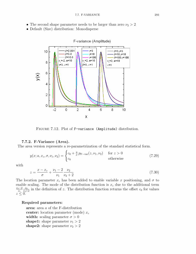
7.7. F-VARIANCE 293
• The second shape parameter needs to be larger than zero ν2 > 2• Default (Size) distribution: Monodisperse
Figure 7.12. Plot of F-variance (Amplitude) distribution.
7.7.2. F-Variance (Area).The area version represents a re-parametrization of the standard statistical form.
y(x; a, xc, σ, ν1, ν2) =
c0 + a
σpF−var(z, ν1, ν2) for z > 0
c0 otherwise(7.29)
with
z =x− xcσ
+ν1 − 2
ν1
ν2
ν2 + 2(7.30)
The location parameter xc has been added to enable variable x positioning, and σ toenable scaling. The mode of the distribution function is xc due to the additional termν1−2ν1
ν2
ν2+2in the definition of z. The distribution function returns the offset c0 for values
z ≤ 0.
Required parameters:
area: area a of the F-distributioncenter: location parameter (mode) xcwidth: scaling parameter σ > 0shape1: shape parameter ν1 > 2shape2: shape parameter ν2 > 2
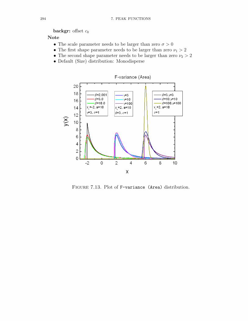
294 7. PEAK FUNCTIONS
backgr: offset c0
Note
• The scale parameter needs to be larger than zero σ > 0• The first shape parameter needs to be larger than zero ν1 > 2• The second shape parameter needs to be larger than zero ν2 > 2• Default (Size) distribution: Monodisperse
Figure 7.13. Plot of F-variance (Area) distribution.

7.8. GAMMA 295
7.8. Gamma
The gamma distribution models sums of exponentially distributed random variables.The gamma distribution family is based on two parameters. The chi-square and ex-
ponential distributions, which are children of the gamma distribution, are one-parameterdistributions that fix one of the two gamma parameters. The standard form is given by
p(x; k, θ) = xk−1 e−x/θ
θk Γ(k)for x > 0 and k, θ > 0. (7.31)
When k is large, the gamma distribution closely approximates a normal distribution withthe advantage that the gamma distribution has density only for positive real numbers.In probability theory and statistics, the gamma distribution is a two-parameter family ofcontinuous probability distributions. It has a scale parameter θ and a shape parameter k.If k is an integer then the distribution represents the sum of k independent exponentiallydistributed random variables, each of which has a mean of θ (which is equivalent to arate parameter of θ−1).
Alternatively, the gamma distribution can be parameterized in terms of a shapeparameter α = k and an inverse scale parameter β = 1/θ, called a rate parameter:
p(x;α, β) = xα−1βα e−β x
Γ(α)for x > 0. (7.32)
7.8.1. Gamma (Amplitude).The parameter xc has been added to enable variable x positioning, whereas the +θ(k−1)
adjusts xc so that it represents the mode. c0 is the offset value. The function returnsthe offset c0 for those x where it is undefined
y(x) =
c0 + a exp(−z)
(z+k−1k−1
)k−1for (z + k − 1) > 0
c0 otherwise(7.33)
with z = x−xcθ
Required parameters:
ampl.: amplitude a of the Gamma peakcenter: location parameter (mode) xcwidth: scaling parameter θ > 0backgr: offset c0
Note
• The shape parameter needs to be larger than one k > 1.• The scale parameter needs to be larger than zero θ > 0• Default (Size) distribution: Monodisperse
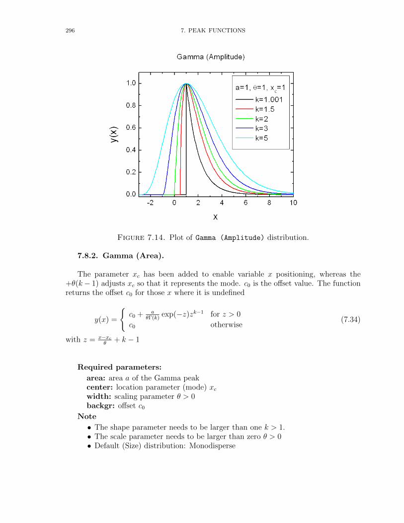
296 7. PEAK FUNCTIONS
Figure 7.14. Plot of Gamma (Amplitude) distribution.
7.8.2. Gamma (Area).
The parameter xc has been added to enable variable x positioning, whereas the+θ(k− 1) adjusts xc so that it represents the mode. c0 is the offset value. The functionreturns the offset c0 for those x where it is undefined
y(x) =
c0 + a
θΓ(k)exp(−z)zk−1 for z > 0
c0 otherwise(7.34)
with z = x−xcθ
+ k − 1
Required parameters:
area: area a of the Gamma peakcenter: location parameter (mode) xcwidth: scaling parameter θ > 0backgr: offset c0
Note
• The shape parameter needs to be larger than one k > 1.• The scale parameter needs to be larger than zero θ > 0• Default (Size) distribution: Monodisperse

7.8. GAMMA 297
Figure 7.15. Plot of Gamma (Area) distribution.
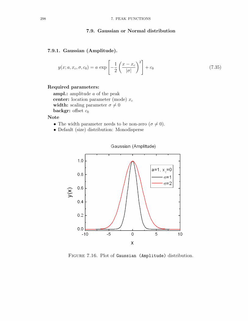
298 7. PEAK FUNCTIONS
7.9. Gaussian or Normal distribution
7.9.1. Gaussian (Amplitude).
y(x; a, xc, σ, c0) = a exp
[−1
2
(x− xc|σ|
)2]
+ c0 (7.35)
Required parameters:
ampl.: amplitude a of the peakcenter: location parameter (mode) xcwidth: scaling parameter σ 6= 0backgr: offset c0
Note
• The width parameter needs to be non-zero (σ 6= 0).• Default (size) distribution: Monodisperse
Figure 7.16. Plot of Gaussian (Amplitude) distribution.
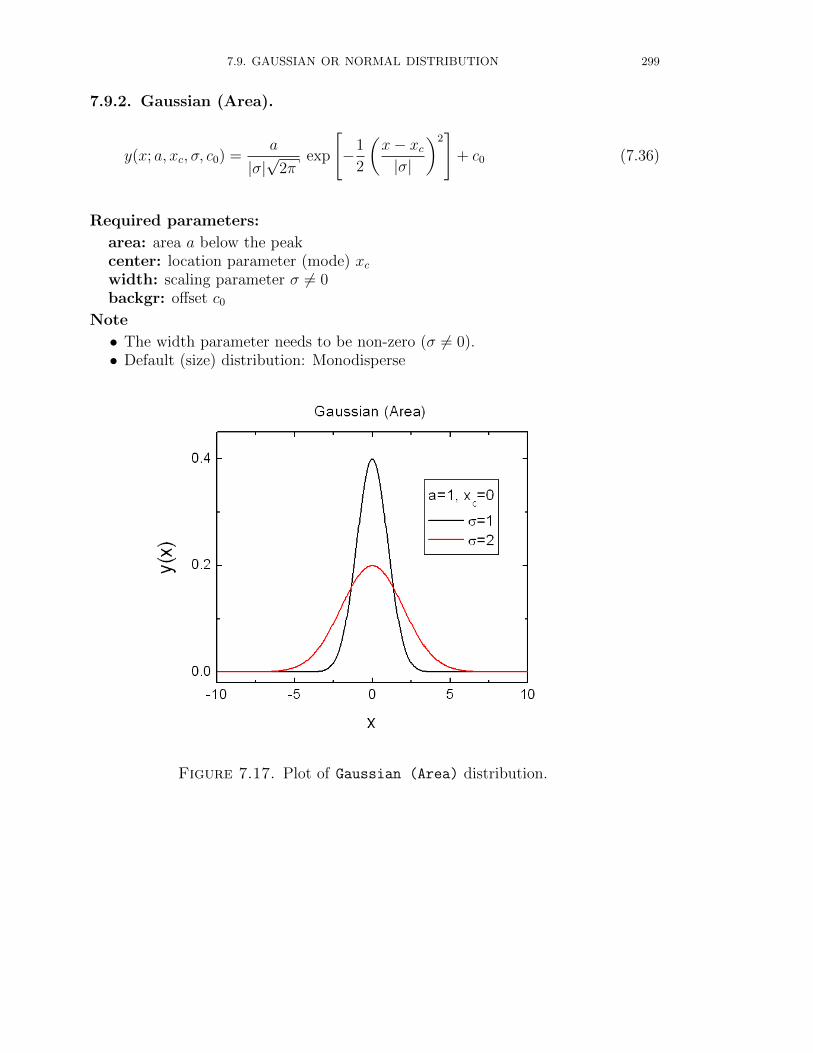
7.9. GAUSSIAN OR NORMAL DISTRIBUTION 299
7.9.2. Gaussian (Area).
y(x; a, xc, σ, c0) =a
|σ|√
2πexp
[−1
2
(x− xc|σ|
)2]
+ c0 (7.36)
Required parameters:
area: area a below the peakcenter: location parameter (mode) xcwidth: scaling parameter σ 6= 0backgr: offset c0
Note
• The width parameter needs to be non-zero (σ 6= 0).• Default (size) distribution: Monodisperse
Figure 7.17. Plot of Gaussian (Area) distribution.
300 7. PEAK FUNCTIONS
7.10. Gaussian-Lorentzian cross product
This distribution function is a Voigt approximation. It combines a Gaussian andLorentzian in a multiplicative form. The shape parameter ν varies from 0 to 1. Thepure Lorentzian occurs with ν = 1 and the pure Gaussian with ν = 0 but the transitionfrom Lorentzian to Gaussian shape in not a linear function of ν
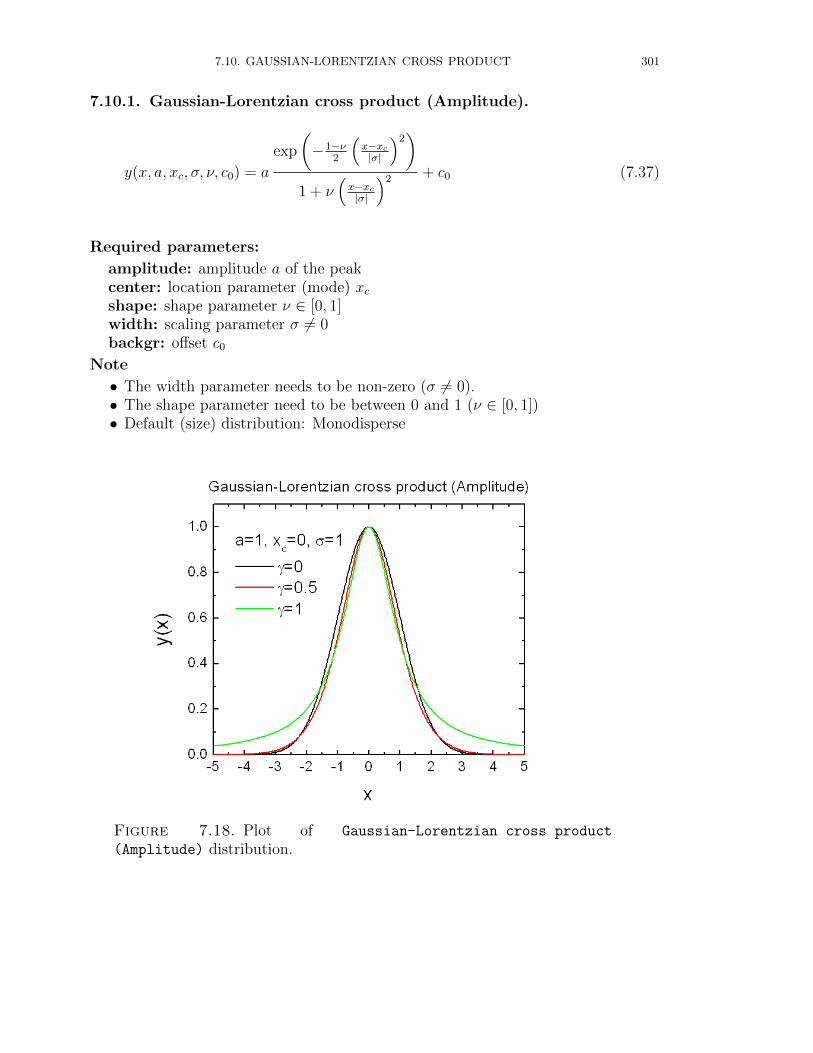
7.10. GAUSSIAN-LORENTZIAN CROSS PRODUCT 301
7.10.1. Gaussian-Lorentzian cross product (Amplitude).
y(x, a, xc, σ, ν, c0) = a
exp
(−1−ν
2
(x−xc|σ|
)2)
1 + ν(x−xc|σ|
)2 + c0 (7.37)
Required parameters:
amplitude: amplitude a of the peakcenter: location parameter (mode) xcshape: shape parameter ν ∈ [0, 1]width: scaling parameter σ 6= 0backgr: offset c0
Note
• The width parameter needs to be non-zero (σ 6= 0).• The shape parameter need to be between 0 and 1 (ν ∈ [0, 1])• Default (size) distribution: Monodisperse
Figure 7.18. Plot of Gaussian-Lorentzian cross product
(Amplitude) distribution.
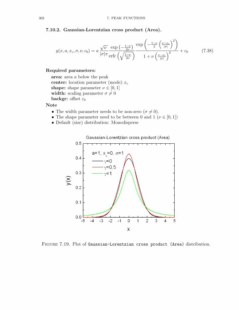
302 7. PEAK FUNCTIONS
7.10.2. Gaussian-Lorentzian cross product (Area).
y(x, a, xc, σ, ν, c0) = a
√ν
|σ|πexp
(−1−ν
2ν
)erfc
(√1−ν2ν
) exp
(−1−ν
2
(x−xc|σ|
)2)
1 + ν(x−xc|σ|
)2 + c0 (7.38)
Required parameters:
area: area a below the peakcenter: location parameter (mode) xcshape: shape parameter ν ∈ [0, 1]width: scaling parameter σ 6= 0backgr: offset c0
Note
• The width parameter needs to be non-zero (σ 6= 0).• The shape parameter need to be between 0 and 1 (ν ∈ [0, 1])• Default (size) distribution: Monodisperse
Figure 7.19. Plot of Gaussian-Lorentzian cross product (Area) distribution.
7.11. GAUSSIAN-LORENTZIAN SUM 303
7.11. Gaussian-Lorentzian sum
This distribution function is another Voigt approximation, which is simply a sum ofLorentzian and Gaussian with equal FWHM. The shape parameter ν varies from 0 to 1.The pure Lorentzian occurs with ν = 1 and the pure Gaussian with ν = 0. The widthparameter σ directly computes the full-width at half-maximum (FWHM).
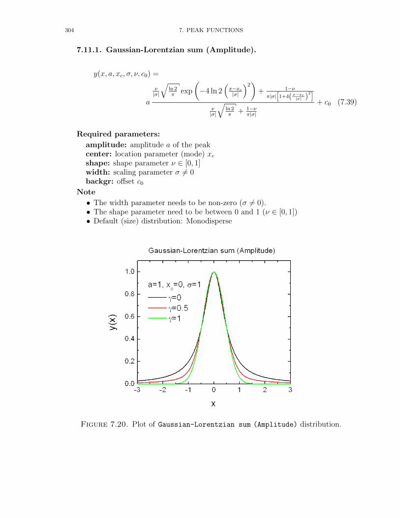
304 7. PEAK FUNCTIONS
7.11.1. Gaussian-Lorentzian sum (Amplitude).
y(x, a, xc, σ, ν, c0) =
a
ν|σ|
√ln 2π
exp
(−4 ln 2
(x−xc|σ|
)2)
+ 1−νπ|σ|
[1+4(x−xc|σ| )
2]
ν|σ|
√ln 2π
+ 1−νπ|σ|
+ c0 (7.39)
Required parameters:
amplitude: amplitude a of the peakcenter: location parameter (mode) xcshape: shape parameter ν ∈ [0, 1]width: scaling parameter σ 6= 0backgr: offset c0
Note
• The width parameter needs to be non-zero (σ 6= 0).• The shape parameter need to be between 0 and 1 (ν ∈ [0, 1])• Default (size) distribution: Monodisperse
Figure 7.20. Plot of Gaussian-Lorentzian sum (Amplitude) distribution.
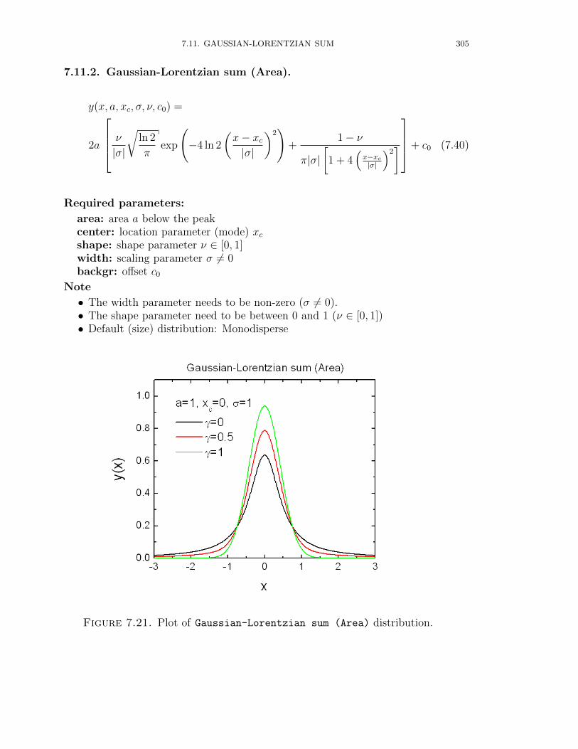
7.11. GAUSSIAN-LORENTZIAN SUM 305
7.11.2. Gaussian-Lorentzian sum (Area).
y(x, a, xc, σ, ν, c0) =
2a
ν
|σ|
√ln 2
πexp
(−4 ln 2
(x− xc|σ|
)2)
+1− ν
π|σ|[1 + 4
(x−xc|σ|
)2]+ c0 (7.40)
Required parameters:
area: area a below the peakcenter: location parameter (mode) xcshape: shape parameter ν ∈ [0, 1]width: scaling parameter σ 6= 0backgr: offset c0
Note
• The width parameter needs to be non-zero (σ 6= 0).• The shape parameter need to be between 0 and 1 (ν ∈ [0, 1])• Default (size) distribution: Monodisperse
Figure 7.21. Plot of Gaussian-Lorentzian sum (Area) distribution.
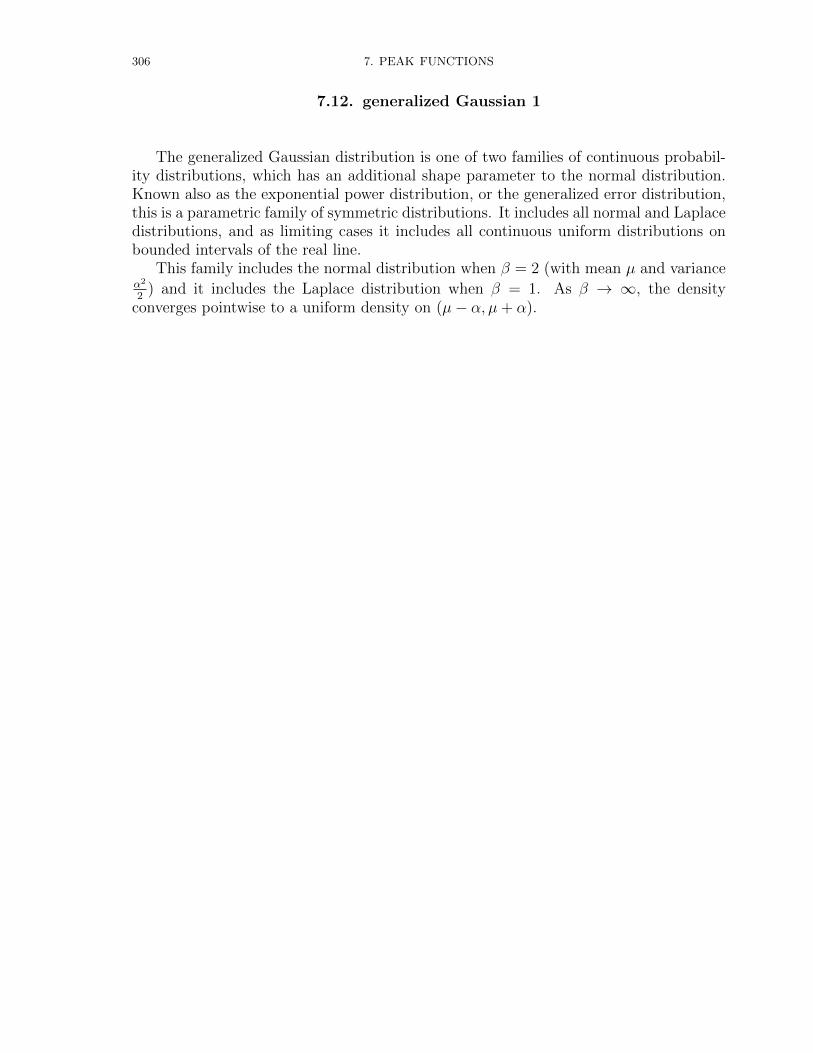
306 7. PEAK FUNCTIONS
7.12. generalized Gaussian 1
The generalized Gaussian distribution is one of two families of continuous probabil-ity distributions, which has an additional shape parameter to the normal distribution.Known also as the exponential power distribution, or the generalized error distribution,this is a parametric family of symmetric distributions. It includes all normal and Laplacedistributions, and as limiting cases it includes all continuous uniform distributions onbounded intervals of the real line.
This family includes the normal distribution when β = 2 (with mean µ and varianceα2
2) and it includes the Laplace distribution when β = 1. As β → ∞, the density
converges pointwise to a uniform density on (µ− α, µ+ α).
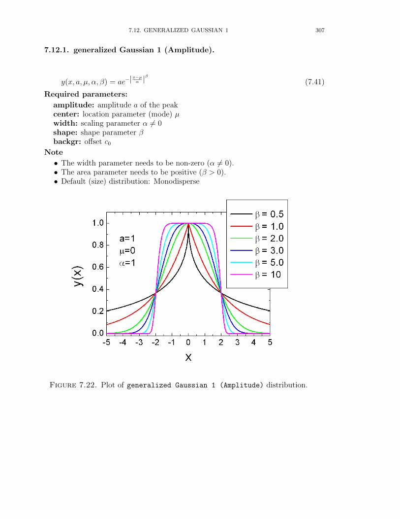
7.12. GENERALIZED GAUSSIAN 1 307
7.12.1. generalized Gaussian 1 (Amplitude).
y(x, a, µ, α, β) = ae−|x−µα |
β
(7.41)
Required parameters:
amplitude: amplitude a of the peakcenter: location parameter (mode) µwidth: scaling parameter α 6= 0shape: shape parameter βbackgr: offset c0
Note
• The width parameter needs to be non-zero (α 6= 0).• The area parameter needs to be positive (β > 0).• Default (size) distribution: Monodisperse
Figure 7.22. Plot of generalized Gaussian 1 (Amplitude) distribution.
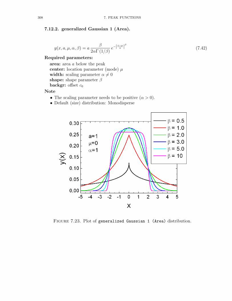
308 7. PEAK FUNCTIONS
7.12.2. generalized Gaussian 1 (Area).
y(x, a, µ, α, β) = aβ
2αΓ (1/β)e−|
x−µα |
β
(7.42)
Required parameters:
area: area a below the peakcenter: location parameter (mode) µwidth: scaling parameter α 6= 0shape: shape parameter βbackgr: offset c0
Note
• The scaling parameter needs to be positive (α > 0).• Default (size) distribution: Monodisperse
Figure 7.23. Plot of generalized Gaussian 1 (Area) distribution.
7.13. GENERALIZED GAUSSIAN 2 309
7.13. generalized Gaussian 2
xmode =
ακ− α
κe−κ
2/2 + ξ if κ 6= 0
ξ if κ = 0(7.43)

310 7. PEAK FUNCTIONS
7.13.1. generalized Gaussian 2 (Amplitude).
y(x) = Aα√
2π exp
(−κ
2
2
)φ(u)
α− κ(x− ξ)+ c0 (7.44)
where
u =
− 1κ
log[1− κ(x−ξ)
α
]if κ 6= 0
x−ξα
if κ = 0(7.45)
where
φ(x) =1√2π
exp
(−x
2
2
)(7.46)
Required parameters:
amplitude: amplitude A of the peaklocation: location parameter ξwidth: scaling parameter α > 0shape: shape parameter κbackgr: offset c0
Note
• The scaling parameter needs to be positive (α > 0).• Default (size) distribution: Monodisperse
Figure 7.24. Plot of generalized Gaussian 2(Amplitude) distribution.
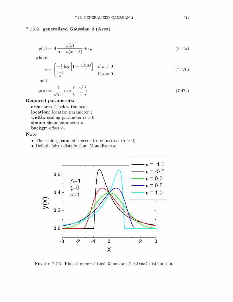
7.13. GENERALIZED GAUSSIAN 2 311
7.13.2. generalized Gaussian 2 (Area).
y(x) = Aφ(u)
α− κ(x− ξ)+ c0 (7.47a)
where
u =
− 1κ
log[1− κ(x−ξ)
α
]if κ 6= 0
x−ξα
if κ = 0(7.47b)
and
φ(u) =1√2π
exp
(−u
2
2
)(7.47c)
Required parameters:
area: area A below the peaklocation: location parameter ξwidth: scaling parameter α > 0shape: shape parameter κbackgr: offset c0
Note
• The scaling parameter needs to be positive (α > 0).• Default (size) distribution: Monodisperse
Figure 7.25. Plot of generalized Gaussian 2 (Area) distribution.
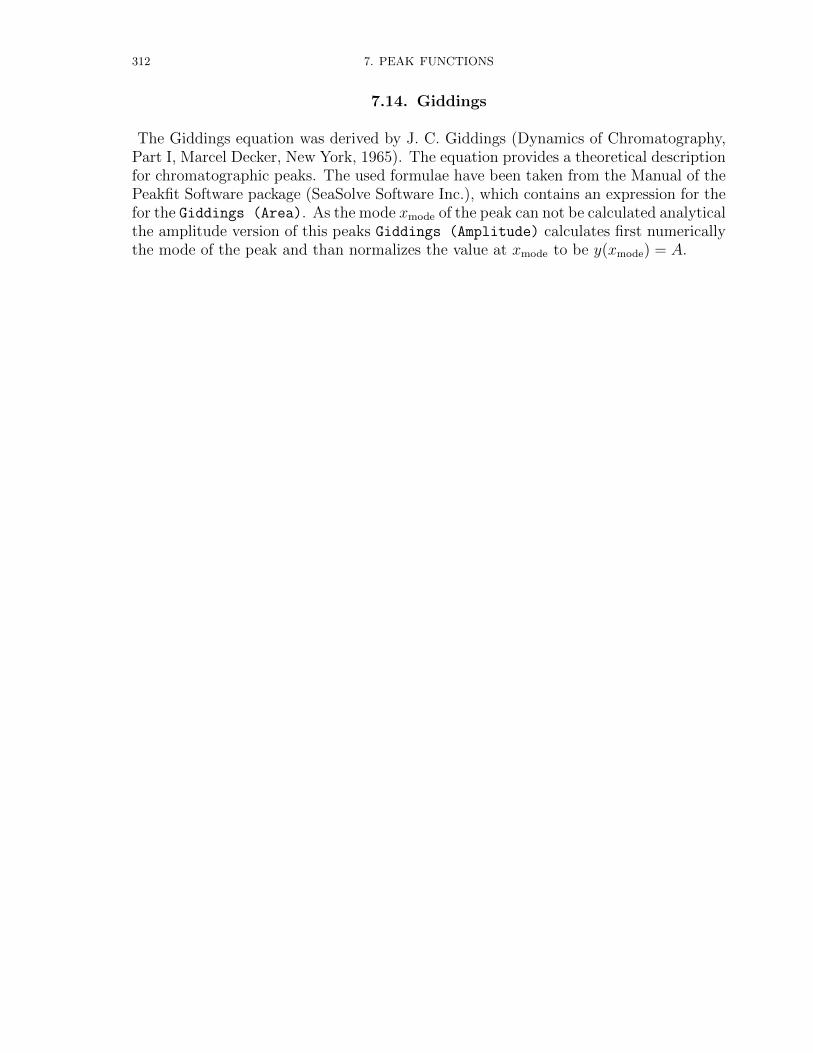
312 7. PEAK FUNCTIONS
7.14. Giddings
The Giddings equation was derived by J. C. Giddings (Dynamics of Chromatography,Part I, Marcel Decker, New York, 1965). The equation provides a theoretical descriptionfor chromatographic peaks. The used formulae have been taken from the Manual of thePeakfit Software package (SeaSolve Software Inc.), which contains an expression for thefor the Giddings (Area). As the mode xmode of the peak can not be calculated analyticalthe amplitude version of this peaks Giddings (Amplitude) calculates first numericallythe mode of the peak and than normalizes the value at xmode to be y(xmode) = A.
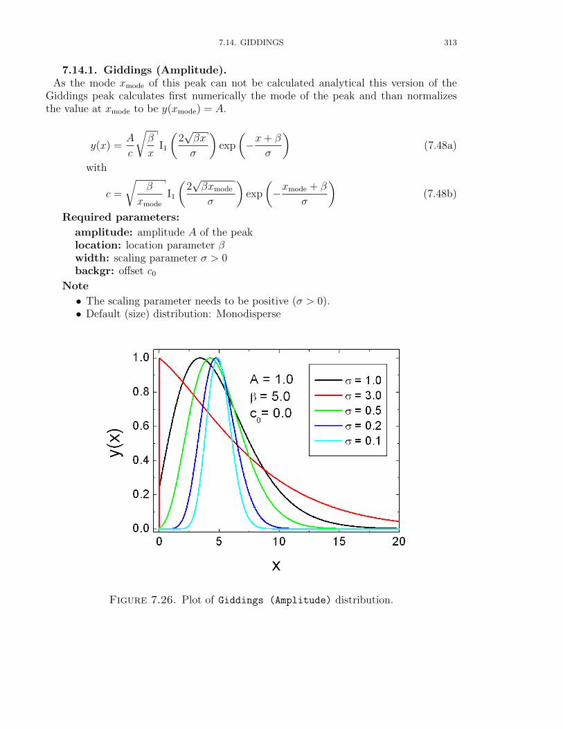
7.14. GIDDINGS 313
7.14.1. Giddings (Amplitude).As the mode xmode of this peak can not be calculated analytical this version of the
Giddings peak calculates first numerically the mode of the peak and than normalizesthe value at xmode to be y(xmode) = A.
y(x) =A
c
√β
xI1
(2√βx
σ
)exp
(−x+ β
σ
)(7.48a)
with
c =
√β
xmode
I1
(2√βxmode
σ
)exp
(−xmode + β
σ
)(7.48b)
Required parameters:
amplitude: amplitude A of the peaklocation: location parameter βwidth: scaling parameter σ > 0backgr: offset c0
Note
• The scaling parameter needs to be positive (σ > 0).• Default (size) distribution: Monodisperse
Figure 7.26. Plot of Giddings (Amplitude) distribution.
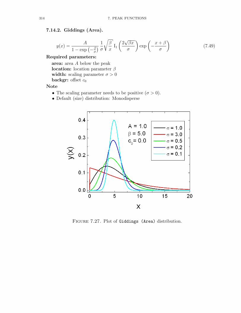
314 7. PEAK FUNCTIONS
7.14.2. Giddings (Area).
y(x) =A
1− exp(−βσ
) 1
σ
√β
xI1
(2√βx
σ
)exp
(−x+ β
σ
)(7.49)
Required parameters:
area: area A below the peaklocation: location parameter βwidth: scaling parameter σ > 0backgr: offset c0
Note
• The scaling parameter needs to be positive (σ > 0).• Default (size) distribution: Monodisperse
Figure 7.27. Plot of Giddings (Area) distribution.

7.15. HAARHOFF - VAN DER LINDE (AREA) 315
7.15. Haarhoff - Van der Linde (Area)
Required parameters:
y(x) =
Aσµδ√
2πexp
[−1
2
(x−µσ
)2]
exp(1− µδ
σ2
)+ 1
2
[1 + erf
(x−µ√
2 σ
)] (7.50)
Required parameters:
area: area A below the peaklocation: location parameter µ > 0width: scaling parameter σ > 0delta: distortion parameter δ 6= 0backgr: offset c0
Note
• The location parameter needs to be positive (µ > 0).• The scaling parameter needs to be positive (σ > 0).• The distortion parameter needs to be nonzero (δ 6= 0).• Default (size) distribution: Monodisperse
Figure 7.28. Plot of HaarhoffVanderLinde (Area) distribution.
316 7. PEAK FUNCTIONS
7.16. Half Gaussian Modified Gaussian (Area)
The Half Gaussian Modified Gaussian (Area) is the mathematical convolutionof a Gaussian with a half-Gaussian response function. There are only two components tothis model, a primary Gaussian, and a response function which convolves or smears theGaussian as in the profiles above. As the width of the half-Gaussian response increases,peaks become more asymmetric or tailed. This function directly fit both tailed andfronted peaks. The transition from tailed to smooth is continuous and occurs at δ = 0.The formula has been taken from the Manual of the Peakfit Software package (SeaSolveSoftware Inc.).
y(x) = Aexp
(−1
2(x−µ)2
σ2+δ2
) [1 + erf
(δ(x−µ)√
2 σ√σ2+δ2
)]√
2π√σ2 + δ2
(7.51)
Required parameters:
area: area A below the peaklocation: location parameter µwidth: scaling parameter σ > 0distortion: distortion parameter δ 6= 0backgr: offset c0
Note
• The scaling parameter needs to be positive (σ > 0).• The distortion parameter needs to be nonzero (δ 6= 0).• Default (size) distribution: Monodisperse

7.16. HALF GAUSSIAN MODIFIED GAUSSIAN (AREA) 317
Figure 7.29. Plot of Half Gaussian Modified Gaussian (Area) distribution.
318 7. PEAK FUNCTIONS
7.17. Inverted Gamma
The inverse gamma distribution is a two-parameter family of continuous probabilitydistributions on the positive real line, which is the distribution of the reciprocal of avariable distributed according to the gamma distribution. The inverse gamma distribu-tion’s probability density function is defined over the support x > 0. The probabilitydensity function is given by
p(x) =βα
Γ(α)x−α−1 exp
(−βx
)(7.52)
the mode xmode of the probabilty function is given by xmode = βα+1
. The shape parameterα needs to be positive and non-zero as well as the scale parameter β (α > 0, β > 0).The SASfit version represents a reparametrization of the standard statistical form. Theparameter µ has been added to enable variable x positioning. Adjustment terms havebeen added so that µ is the mode xmode. The function returns c0 for those x where it isundefined. Note that the amplitude form is much faster.
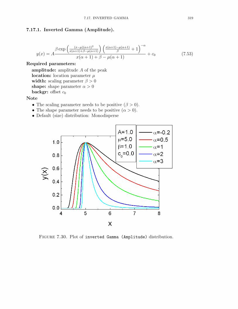
7.17. INVERTED GAMMA 319
7.17.1. Inverted Gamma (Amplitude).
y(x) = Aβ exp
((x−µ)(α+1)2
x(α+1)+β−µ(α+1)
)(x(α+1)−µ(α+1)
β+ 1)−α
x(α + 1) + β − µ(α + 1)+ c0 (7.53)
Required parameters:
amplitude: amplitude A of the peaklocation: location parameter µwidth: scaling parameter β > 0shape: shape parameter α > 0backgr: offset c0
Note
• The scaling parameter needs to be positive (β > 0).• The shape parameter needs to be positive (α > 0).• Default (size) distribution: Monodisperse
Figure 7.30. Plot of inverted Gamma (Amplitude) distribution.
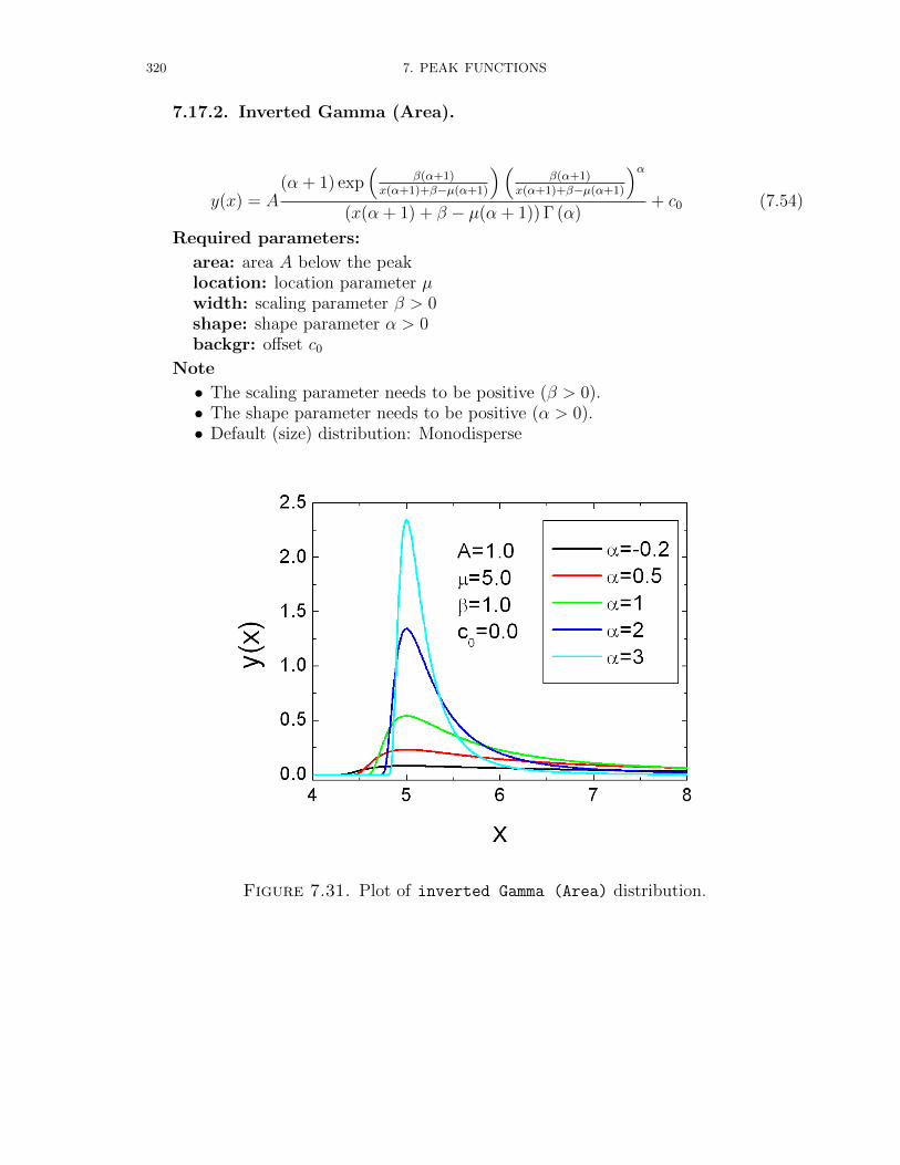
320 7. PEAK FUNCTIONS
7.17.2. Inverted Gamma (Area).
y(x) = A(α + 1) exp
(β(α+1)
x(α+1)+β−µ(α+1)
)(β(α+1)
x(α+1)+β−µ(α+1)
)α(x(α + 1) + β − µ(α + 1)) Γ (α)
+ c0 (7.54)
Required parameters:
area: area A below the peaklocation: location parameter µwidth: scaling parameter β > 0shape: shape parameter α > 0backgr: offset c0
Note
• The scaling parameter needs to be positive (β > 0).• The shape parameter needs to be positive (α > 0).• Default (size) distribution: Monodisperse
Figure 7.31. Plot of inverted Gamma (Area) distribution.

7.18. KUMARASWAMY 321
7.18. Kumaraswamy
The Kumaraswamy’s double bounded distribution is a family of continuous probabilitydistributions defined on the interval [0, 1] differing in the values of their two non-negativeshape parameters, a and b. It is similar to the Beta distribution, but much simpler touse especially in simulation studies due to the simple closed form of both its probabilitydensity function and cumulative distribution function. The probability density functionof the Kumaraswamy distribution is
p(x;α, β) = αβxα−1(1− xα)β−1. (7.55)
For α > 1 and β > 1 the mode of the distribution reads as
xmode =
(α− 1
αβ − 1
)1/α
(7.56)
7.18.1. Kumaraswamy (Amplitude).
y(x) =
Aαβ(
x+xminxmax−xmin
)α−1(1−(
x+xminxmax−xmin
)α)β−1
αβxα−1mode(1−xαmode)β−1 + c0 for x ∈ [xmin, xmax]
c0 for x /∈ [xmin, xmax](7.57)
Required parameters:
ampl.: amplitude A of the Kumaraswamy peakxmin: continuous lower boundary parameters xmin
xmax: continuous upper boundary parameters xmax
alpha: first shape parameter α > 1beta: second shape parameter β > 1backgr: offset c0
Note
• Both shape parameter needs to be larger than one (α, β > 1), as only than thedistribution has a peak shape.• where the Kumaraswamy distribution is not defined the offset value is returned:∀x /∈ (xmin, xmax) yBeta(ampl)(x) = c0
• Default (size) distribution: Monodisperse
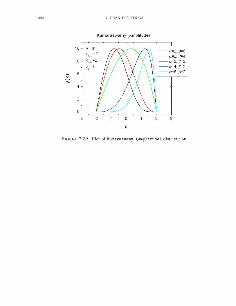
322 7. PEAK FUNCTIONS
Figure 7.32. Plot of Kumaraswamy (Amplitude) distribution.
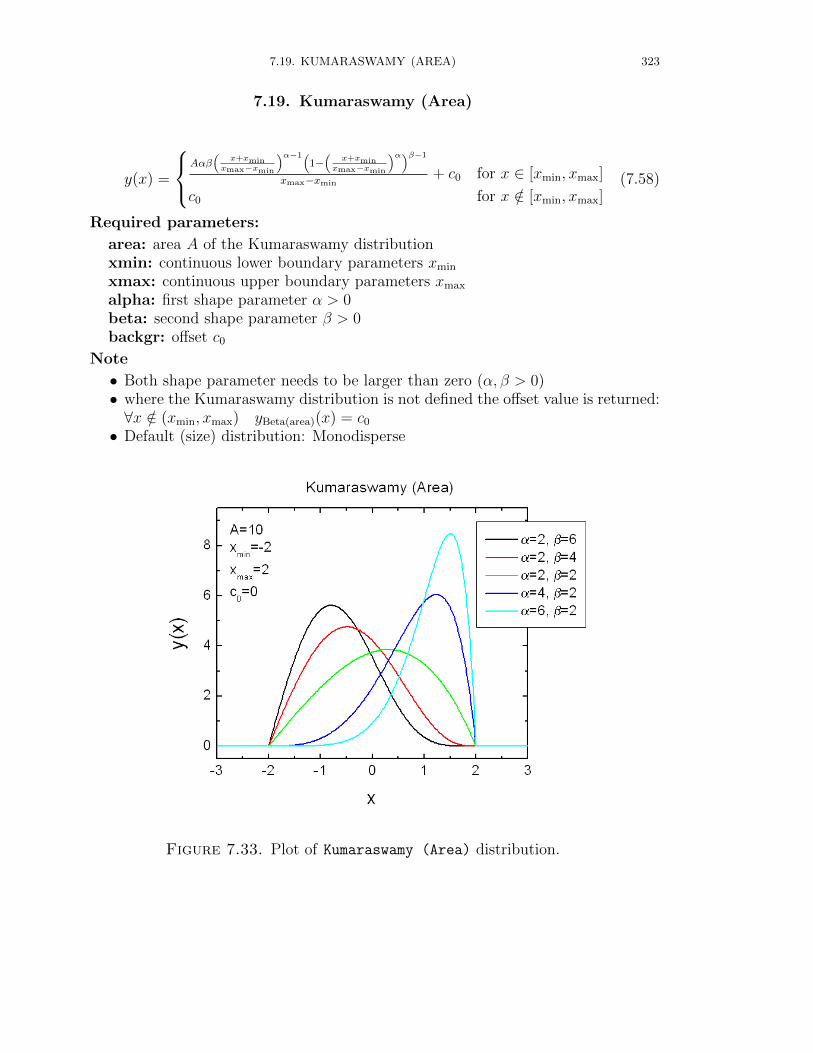
7.19. KUMARASWAMY (AREA) 323
7.19. Kumaraswamy (Area)
y(x) =
Aαβ(
x+xminxmax−xmin
)α−1(1−(
x+xminxmax−xmin
)α)β−1
xmax−xmin+ c0 for x ∈ [xmin, xmax]
c0 for x /∈ [xmin, xmax](7.58)
Required parameters:
area: area A of the Kumaraswamy distributionxmin: continuous lower boundary parameters xmin
xmax: continuous upper boundary parameters xmax
alpha: first shape parameter α > 0beta: second shape parameter β > 0backgr: offset c0
Note
• Both shape parameter needs to be larger than zero (α, β > 0)• where the Kumaraswamy distribution is not defined the offset value is returned:∀x /∈ (xmin, xmax) yBeta(area)(x) = c0
• Default (size) distribution: Monodisperse
Figure 7.33. Plot of Kumaraswamy (Area) distribution.
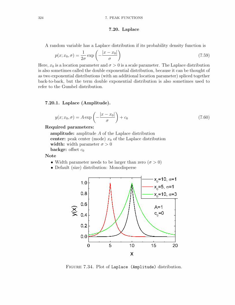
324 7. PEAK FUNCTIONS
7.20. Laplace
A random variable has a Laplace distribution if its probability density function is
p(x;x0, σ) =1
2σexp
(−|x− x0|
σ
)(7.59)
Here, x0 is a location parameter and σ > 0 is a scale parameter. The Laplace distributionis also sometimes called the double exponential distribution, because it can be thought ofas two exponential distributions (with an additional location parameter) spliced togetherback-to-back, but the term double exponential distribution is also sometimes used torefer to the Gumbel distribution.
7.20.1. Laplace (Amplitude).
y(x;x0, σ) = A exp
(−|x− x0|
σ
)+ c0 (7.60)
Required parameters:
amplitude: amplitude A of the Laplace distributioncenter: peak center (mode) x0 of the Laplace distributionwidth: width parameter σ > 0backgr: offset c0
Note
• Width parameter needs to be larger than zero (σ > 0)• Default (size) distribution: Monodisperse
Figure 7.34. Plot of Laplace (Amplitude) distribution.
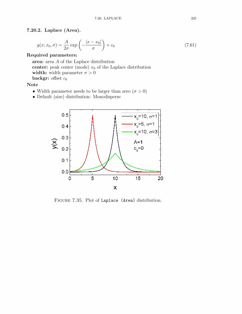
7.20. LAPLACE 325
7.20.2. Laplace (Area).
y(x;x0, σ) =A
2σexp
(−|x− x0|
σ
)+ c0 (7.61)
Required parameters:
area: area A of the Laplace distributioncenter: peak center (mode) x0 of the Laplace distributionwidth: width parameter σ > 0backgr: offset c0
Note
• Width parameter needs to be larger than zero (σ > 0)• Default (size) distribution: Monodisperse
Figure 7.35. Plot of Laplace (Area) distribution.
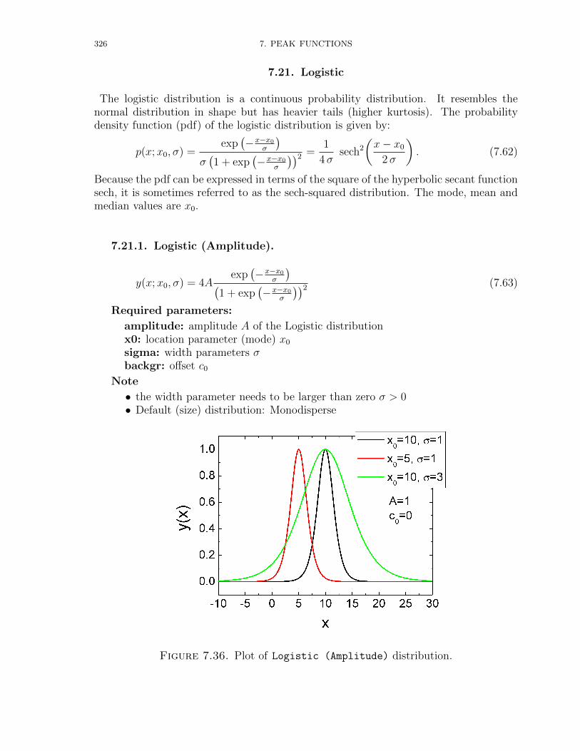
326 7. PEAK FUNCTIONS
7.21. Logistic
The logistic distribution is a continuous probability distribution. It resembles thenormal distribution in shape but has heavier tails (higher kurtosis). The probabilitydensity function (pdf) of the logistic distribution is given by:
p(x;x0, σ) =exp
(−x−x0
σ
)σ(1 + exp
(−x−x0
σ
))2 =1
4σsech2
(x− x0
2σ
). (7.62)
Because the pdf can be expressed in terms of the square of the hyperbolic secant functionsech, it is sometimes referred to as the sech-squared distribution. The mode, mean andmedian values are x0.
7.21.1. Logistic (Amplitude).
y(x;x0, σ) = 4Aexp
(−x−x0
σ
)(1 + exp
(−x−x0
σ
))2 (7.63)
Required parameters:
amplitude: amplitude A of the Logistic distributionx0: location parameter (mode) x0
sigma: width parameters σbackgr: offset c0
Note
• the width parameter needs to be larger than zero σ > 0• Default (size) distribution: Monodisperse
Figure 7.36. Plot of Logistic (Amplitude) distribution.

7.21. LOGISTIC 327
7.21.2. Logistic (Area).
y(x;x0, σ) = Aexp
(−x−x0
σ
)σ(1 + exp
(−x−x0
σ
))2 (7.64)
Required parameters:
area: area A of the Logistic distributionx0: location parameter (mode) x0
sigma: width parameters σbackgr: offset c0
Note
• the width parameter needs to be larger than zero σ > 0• Default (size) distribution: Monodisperse
Figure 7.37. Plot of Logistic (Area) distribution.

328 7. PEAK FUNCTIONS
7.22. LogLogistic
As may be indicated by the name, the loglogistic (known as the Fisk distribution ineconomics) distribution has certain similarities to the logistic distribution. A randomvariable is loglogistically distributed if the logarithm of the random variable is logisti-cally distributed. The LogLogistic distribution is a two-parameter distribution withparameters σ and x0. It is similar in shape to the log-normal distribution but has heaviertails.
The pdf for this distribution is given by:
p(x;µ, σ) =exp
(− log(x)−log(µ)
σ
)σ (x)
(1 + exp
(− log(x)−log(µ)
σ
))2 =
(xµ
)−1/σ
xσ
[1 +
(xµ
)−1/σ]2 . (7.65)
where 0 < x < ∞, −∞ < x0 < ∞ and 0 < σ < ∞. The mode of the LogLogistic
distribution, if σ < 1, is given by:
mode = µ
(1− σ1 + σ
)σ(7.66)
7.22.1. LogLogistic (Amplitude).
y(x) =
A
(x−x0µ )
−1/σ
(x−x0)σ
[1+(x−x0
µ )−1/σ
]2 + c0 for x ≥ x0
c0 for x < x0
(7.67)
Required parameters:
amplitude: amplitude A of the LogLogistic distributionx0: location parameter x0
mu: scale parameter µsigma: shape parameters σbackgr: offset c0
Note
• the width parameter needs to be larger than zero 0 < σ < 1• Default (size) distribution: Monodisperse
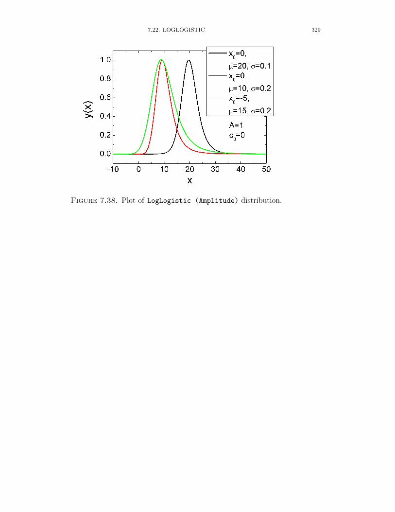
7.22. LOGLOGISTIC 329
Figure 7.38. Plot of LogLogistic (Amplitude) distribution.
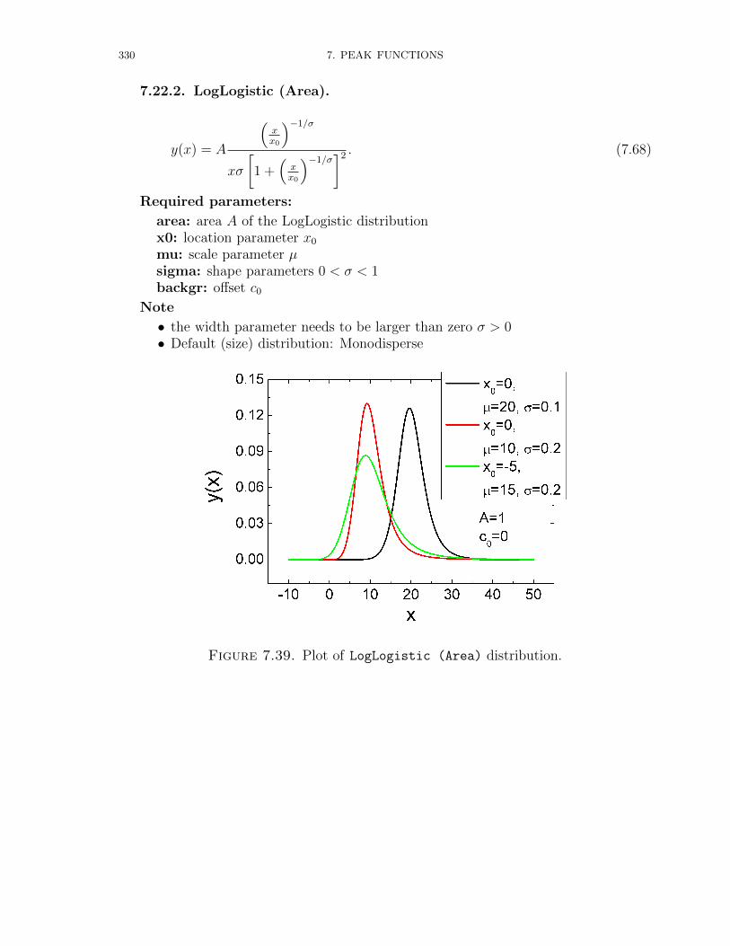
330 7. PEAK FUNCTIONS
7.22.2. LogLogistic (Area).
y(x) = A
(xx0
)−1/σ
xσ
[1 +
(xx0
)−1/σ]2 . (7.68)
Required parameters:
area: area A of the LogLogistic distributionx0: location parameter x0
mu: scale parameter µsigma: shape parameters 0 < σ < 1backgr: offset c0
Note
• the width parameter needs to be larger than zero σ > 0• Default (size) distribution: Monodisperse
Figure 7.39. Plot of LogLogistic (Area) distribution.
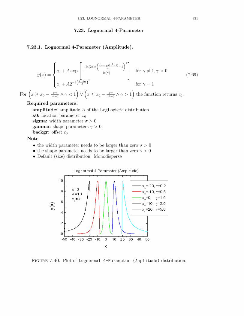
7.23. LOGNORMAL 4-PARAMETER 331
7.23. Lognormal 4-Parameter
7.23.1. Lognormal 4-Parameter (Amplitude).
y(x) =
c0 + A exp
− ln(2) ln
((x−x0)(γ2−1)
σγ+1
)2
ln(γ)
for γ 6= 1, γ > 0
c0 + A2−4(x−x0σ )
2
for γ = 1
(7.69)
For(x ≥ x0 − σγ
γ2−1∧ γ < 1
)∨(x ≤ x0 − σγ
γ2−1∧ γ > 1
)the function returns c0.
Required parameters:
amplitude: amplitude A of the LogLogistic distributionx0: location parameter x0
sigma: width parameter σ > 0gamma: shape parameters γ > 0backgr: offset c0
Note
• the width parameter needs to be larger than zero σ > 0• the shape parameter needs to be larger than zero γ > 0• Default (size) distribution: Monodisperse
Figure 7.40. Plot of Lognormal 4-Parameter (Amplitude) distribution.
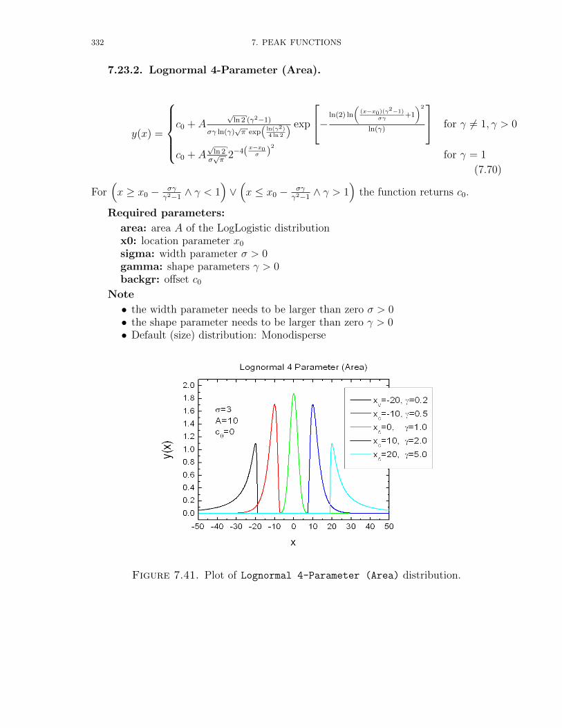
332 7. PEAK FUNCTIONS
7.23.2. Lognormal 4-Parameter (Area).
y(x) =
c0 + A
√ln 2 (γ2−1)
σγ ln(γ)√π exp
(ln(γ2)4 ln 2
) exp
− ln(2) ln
((x−x0)(γ2−1)
σγ+1
)2
ln(γ)
for γ 6= 1, γ > 0
c0 + A√
ln 2σ√π
2−4(x−x0σ )
2
for γ = 1
(7.70)
For(x ≥ x0 − σγ
γ2−1∧ γ < 1
)∨(x ≤ x0 − σγ
γ2−1∧ γ > 1
)the function returns c0.
Required parameters:
area: area A of the LogLogistic distributionx0: location parameter x0
sigma: width parameter σ > 0gamma: shape parameters γ > 0backgr: offset c0
Note
• the width parameter needs to be larger than zero σ > 0• the shape parameter needs to be larger than zero γ > 0• Default (size) distribution: Monodisperse
Figure 7.41. Plot of Lognormal 4-Parameter (Area) distribution.
7.24. LOGNORMAL 333
7.24. LogNormal
The LogNormal distribution is defined with reference to the normal distribution. Arandom variable is Lognormally distributed if the logarithm of the random variable isnormally distributed.
The LogNormal distribution is commonly used for general reliability analysis, cycles-to-failure in fatigue, material strengths and loading variables in probabilistic design.Another advantage of the LogNormal distribution is that it is positive-definite, so it isoften useful for representing quantities that cannot have negative values. LogNormaldistributions have proven useful as distributions for rainfall amounts, for the size dis-tributions of aerosol particles or droplets, and for many other cases. The log-normaldistribution has the probability density function
f(x′) =1
σ√
2πexp
(−1
2
(x′ − µ′
σ
)2)
(7.71)
where µ′ = ln(µ) and x′ = ln(x). The lognormal pdf can be obtained, realizing that forequal probabilities under the normal and lognormal pdfs, incremental areas should alsobe equal, or:
f(x;µ, σ)dx = f(x′;µ, σ)dx′ (7.72)
Taking the derivative yields:
dx′ =dx
x(7.73)
Substitution yields:
f(x;µ, σ) =f(x′;µ, σ)
x(7.74)
where:
f(x;µ, σ) =1
xσ√
2πexp
(−1
2
(ln(x)− ln(µ)
σ
)2)
(7.75)
for x ∈ (0,∞], where µ > 0 and σ 6= 0 are the location and scale parameter. The modeof the distribution is
mode = µ exp(−σ2
)(7.76)
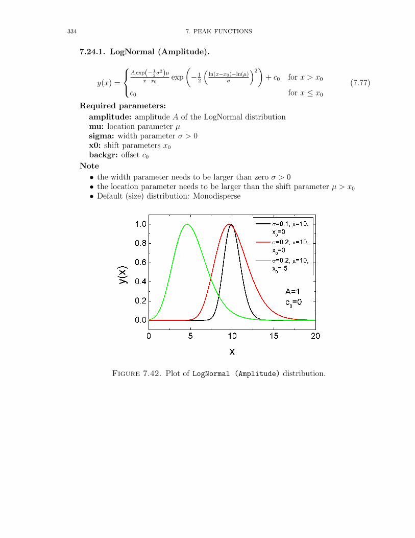
334 7. PEAK FUNCTIONS
7.24.1. LogNormal (Amplitude).
y(x) =
A exp(− 1
2σ2)µ
x−x0exp
(−1
2
(ln(x−x0)−ln(µ)
σ
)2)
+ c0 for x > x0
c0 for x ≤ x0
(7.77)
Required parameters:
amplitude: amplitude A of the LogNormal distributionmu: location parameter µsigma: width parameter σ > 0x0: shift parameters x0
backgr: offset c0
Note
• the width parameter needs to be larger than zero σ > 0• the location parameter needs to be larger than the shift parameter µ > x0
• Default (size) distribution: Monodisperse
Figure 7.42. Plot of LogNormal (Amplitude) distribution.
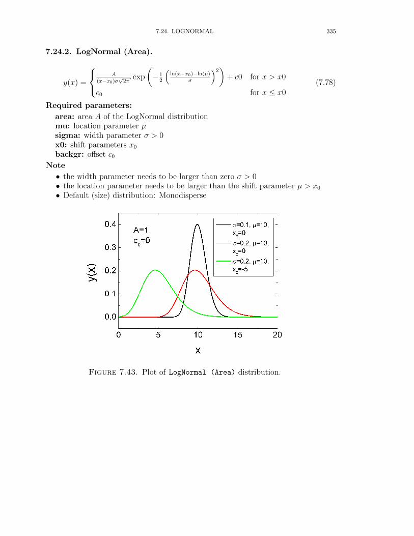
7.24. LOGNORMAL 335
7.24.2. LogNormal (Area).
y(x) =
A(x−x0)σ
√2π
exp
(−1
2
(ln(x−x0)−ln(µ)
σ
)2)
+ c0 for x > x0
c0 for x ≤ x0(7.78)
Required parameters:
area: area A of the LogNormal distributionmu: location parameter µsigma: width parameter σ > 0x0: shift parameters x0
backgr: offset c0
Note
• the width parameter needs to be larger than zero σ > 0• the location parameter needs to be larger than the shift parameter µ > x0
• Default (size) distribution: Monodisperse
Figure 7.43. Plot of LogNormal (Area) distribution.

336 7. PEAK FUNCTIONS
7.25. Lorentzian or Cauchy distribution
The CauchyLorentz Distribution, named after Augustin Cauchy and HendrikLorentz, is a continuous probability distribution. As a probability distribution, it isknown as the Cauchy distribution, while among physicists, it is known as a Lorentzdistribution, or a Lorentz(ian) function or the BreitWigner distribution. Its importancein physics is due to it being the solution to the differential equation describing forcedresonance. The Lorntzian distribution has the probability density function
f(x;x0, σ) =1
πσ[1 +
(x−x0
σ
)2]
=1
π
[σ
(x− x0)2 + σ2
](7.79)
where x0 is the location parameter, specifying the location of the peak of the distribution,and σ is the scale parameter which specifies the half-width at half-maximum (HWHM).
7.25.1. Lorentzian (Amplitude).
Figure 7.44. Plot of Lorentzian (Amplitude) distribution.
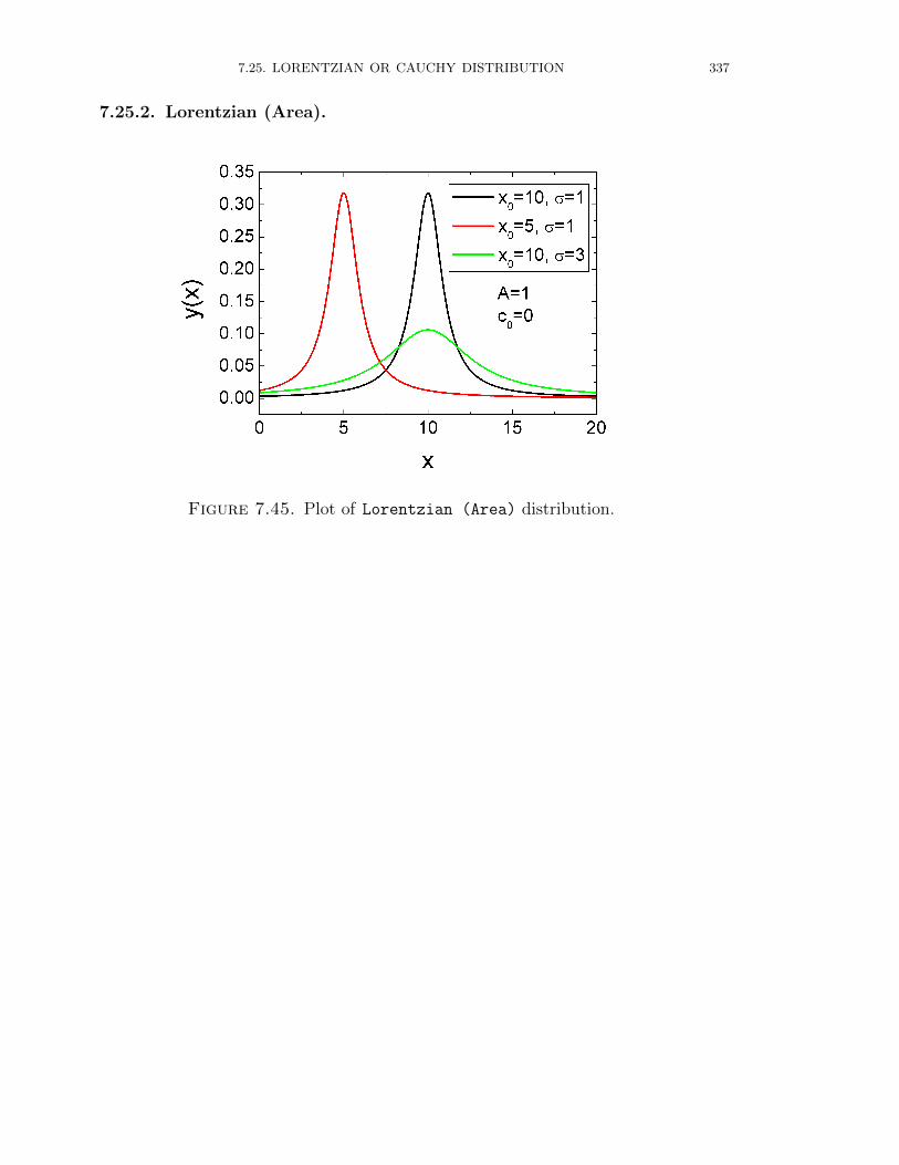
7.25. LORENTZIAN OR CAUCHY DISTRIBUTION 337
7.25.2. Lorentzian (Area).
Figure 7.45. Plot of Lorentzian (Area) distribution.
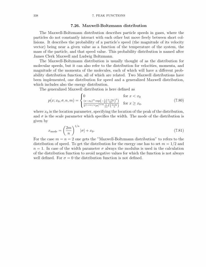
338 7. PEAK FUNCTIONS
7.26. Maxwell-Boltzmann distribution
The Maxwell-Boltzmann distribution describes particle speeds in gases, where theparticles do not constantly interact with each other but move freely between short col-lisions. It describes the probability of a particle’s speed (the magnitude of its velocityvector) being near a given value as a function of the temperature of the system, themass of the particle, and that speed value. This probability distribution is named afterJames Clerk Maxwell and Ludwig Boltzmann.
The Maxwell-Boltzmann distribution is usually thought of as the distribution formolecular speeds, but it can also refer to the distribution for velocities, momenta, andmagnitude of the momenta of the molecules, each of which will have a different prob-ability distribution function, all of which are related. Two Maxwell distributions havebeen implemented, one distribution for speed and a generalized Maxwell distribution,which includes also the energy distribution.
The generalized Maxwell distribution is here defined as
p(x;x0, σ, n,m) =
0 for x < x0
(x−x0)m exp(− 12(x−x0
|σ| )n)
2(1+m)/n|σ|1+m 1|n|Γ( 1+m
n )for x ≥ x0.
(7.80)
where x0 is the location parameter, specifying the location of the peak of the distribution,and σ is the scale parameter which specifies the width. The mode of the distribution isgiven by
xmode =
(2m
n
)1/n
|σ|+ x0. (7.81)
For the case m = n = 2 one gets the ”Maxwell-Boltzmann distribution” to refers to thedistribution of speed. To get the distribution for the energy one has to set m = 1/2 andn = 1. In case of the width parameter σ always the modulus is used in the calculationof the distribution function to avoid negative values for which the function is not alwayswell defined. For σ = 0 the distribution function is not defined.
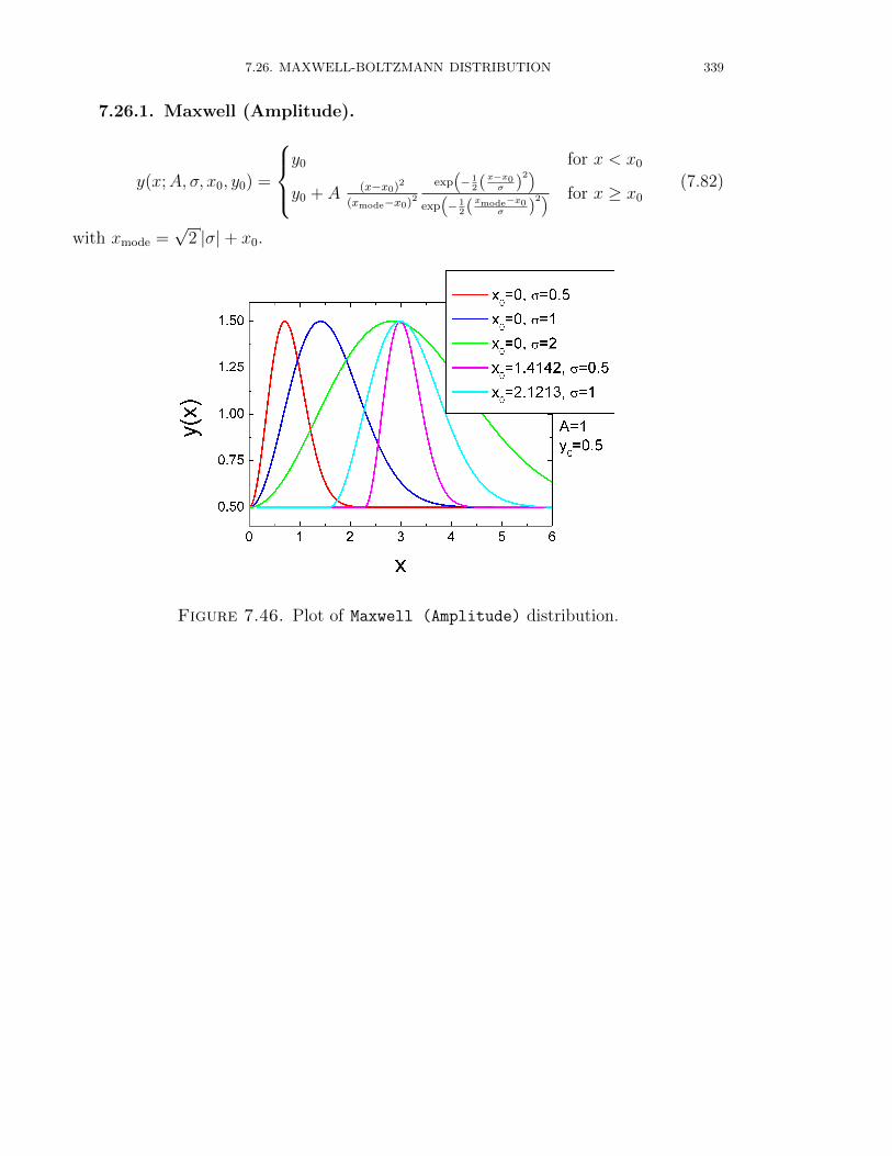
7.26. MAXWELL-BOLTZMANN DISTRIBUTION 339
7.26.1. Maxwell (Amplitude).
y(x;A, σ, x0, y0) =
y0 for x < x0
y0 + A (x−x0)2
(xmode−x0)2
exp(− 1
2(x−x0σ )
2)
exp(− 1
2(xmode−x0σ )
2) for x ≥ x0
(7.82)
with xmode =√
2 |σ|+ x0.
Figure 7.46. Plot of Maxwell (Amplitude) distribution.
340 7. PEAK FUNCTIONS
7.26.2. Maxwell (Area).
y(x;A, σ, x0, y0) =
y0 for x < x0
y0 +√
2πA(x−x0)2
σ3 exp(−1
2
(x−x0
σ
)2)
for x ≥ x0
(7.83)
Figure 7.47. Plot of Maxwell (Area) distribution.
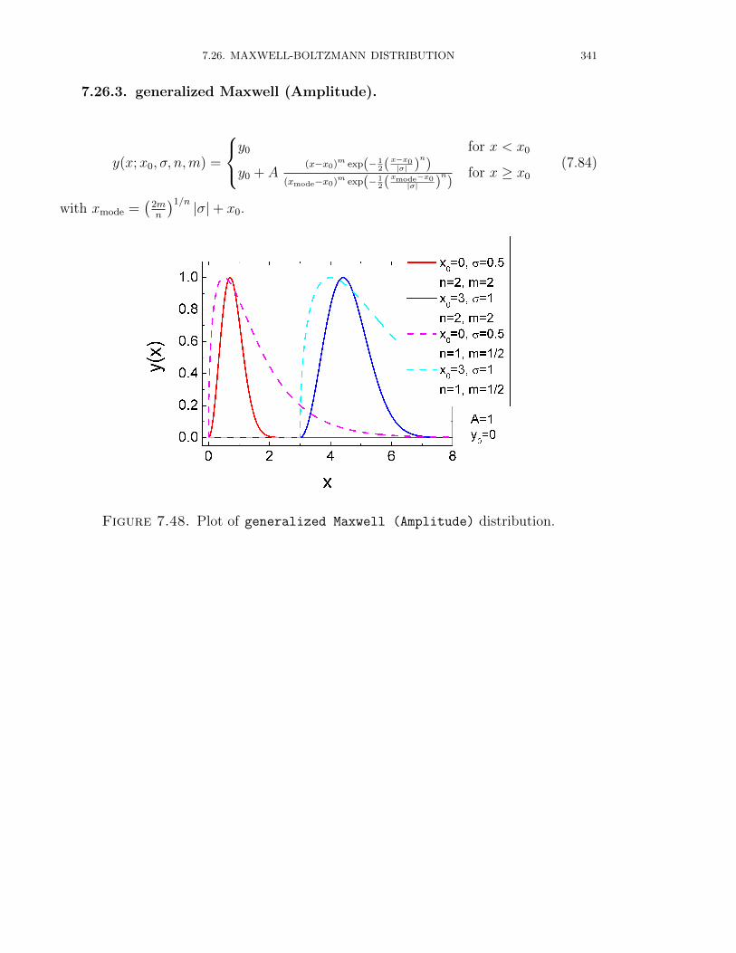
7.26. MAXWELL-BOLTZMANN DISTRIBUTION 341
7.26.3. generalized Maxwell (Amplitude).
y(x;x0, σ, n,m) =
y0 for x < x0
y0 + A(x−x0)m exp(− 1
2(x−x0|σ| )
n)
(xmode−x0)m exp(− 12(xmode−x0
|σ| )n)
for x ≥ x0
(7.84)
with xmode =(
2mn
)1/n |σ|+ x0.
Figure 7.48. Plot of generalized Maxwell (Amplitude) distribution.
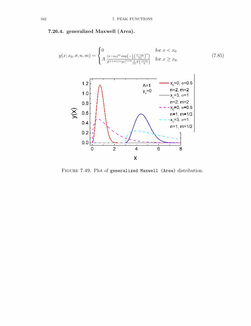
342 7. PEAK FUNCTIONS
7.26.4. generalized Maxwell (Area).
y(x;x0, σ, n,m) =
0 for x < x0
A(x−x0)m exp(− 1
2(x−x0|σ| )
n)
2(1+m)/n|σ|1+m 1|n|Γ( 1+m
n )for x ≥ x0.
(7.85)
Figure 7.49. Plot of generalized Maxwell (Area) distribution.
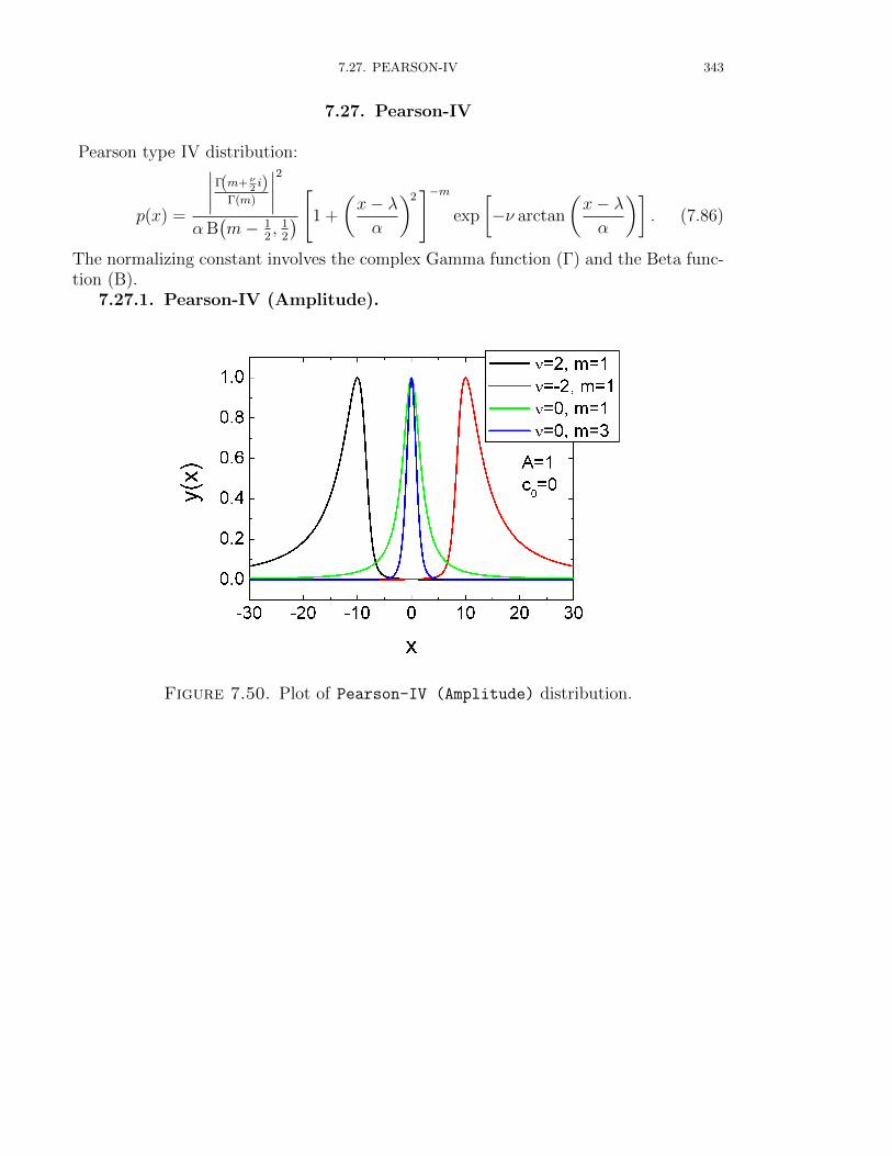
7.27. PEARSON-IV 343
7.27. Pearson-IV
Pearson type IV distribution:
p(x) =
∣∣∣∣Γ(m+ ν2i)
Γ(m)
∣∣∣∣2αB(m− 1
2, 1
2
) [1 +
(x− λα
)2]−m
exp
[−ν arctan
(x− λα
)]. (7.86)
The normalizing constant involves the complex Gamma function (Γ) and the Beta func-tion (B).
7.27.1. Pearson-IV (Amplitude).
Figure 7.50. Plot of Pearson-IV (Amplitude) distribution.
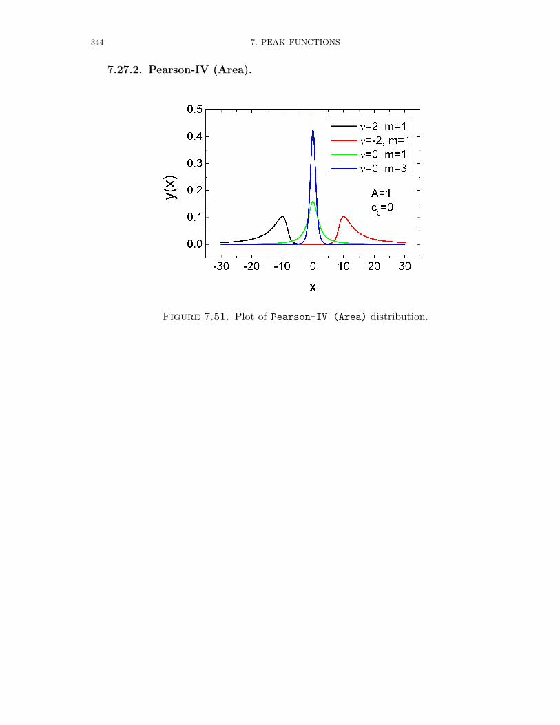
344 7. PEAK FUNCTIONS
7.27.2. Pearson-IV (Area).
Figure 7.51. Plot of Pearson-IV (Area) distribution.
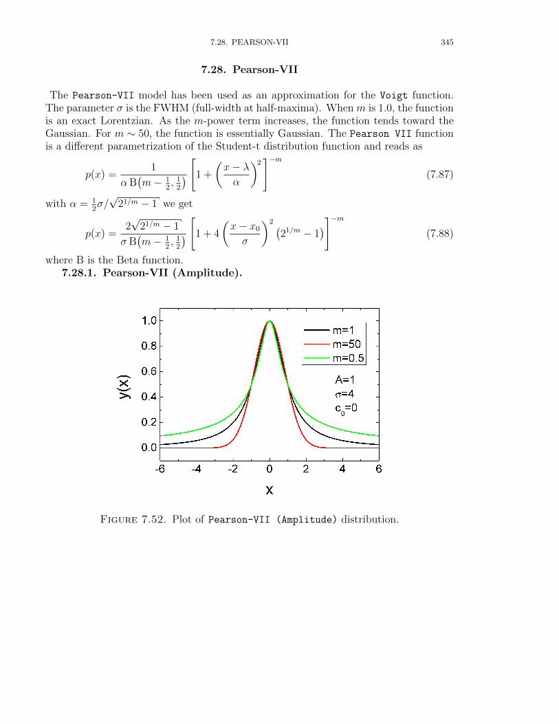
7.28. PEARSON-VII 345
7.28. Pearson-VII
The Pearson-VII model has been used as an approximation for the Voigt function.The parameter σ is the FWHM (full-width at half-maxima). When m is 1.0, the functionis an exact Lorentzian. As the m-power term increases, the function tends toward theGaussian. For m ∼ 50, the function is essentially Gaussian. The Pearson VII functionis a different parametrization of the Student-t distribution function and reads as
p(x) =1
αB(m− 1
2, 1
2
) [1 +
(x− λα
)2]−m
(7.87)
with α = 12σ/√
21/m − 1 we get
p(x) =2√
21/m − 1
σB(m− 1
2, 1
2
) [1 + 4
(x− x0
σ
)2 (21/m − 1
)]−m(7.88)
where B is the Beta function.7.28.1. Pearson-VII (Amplitude).
Figure 7.52. Plot of Pearson-VII (Amplitude) distribution.
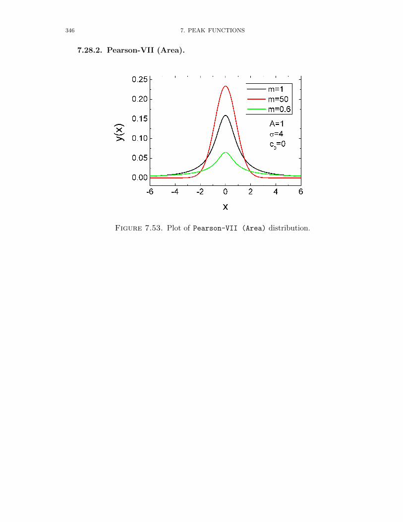
346 7. PEAK FUNCTIONS
7.28.2. Pearson-VII (Area).
Figure 7.53. Plot of Pearson-VII (Area) distribution.
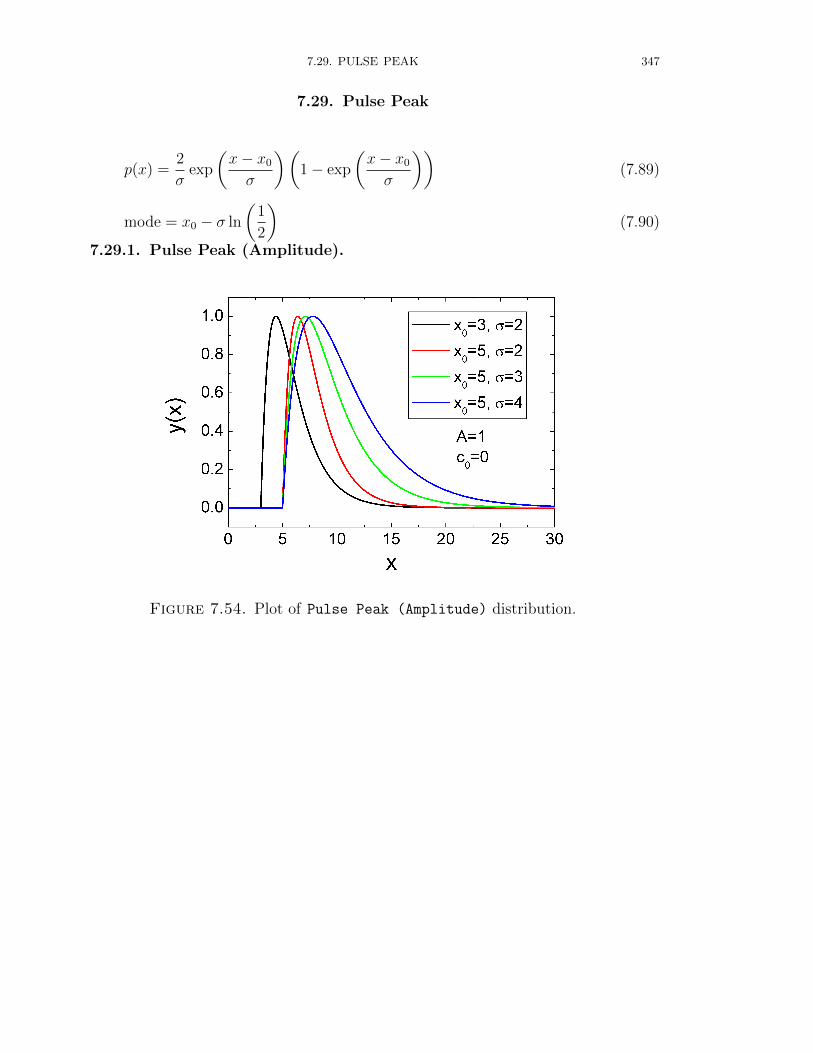
7.29. PULSE PEAK 347
7.29. Pulse Peak
p(x) =2
σexp
(x− x0
σ
)(1− exp
(x− x0
σ
))(7.89)
mode = x0 − σ ln
(1
2
)(7.90)
7.29.1. Pulse Peak (Amplitude).
Figure 7.54. Plot of Pulse Peak (Amplitude) distribution.
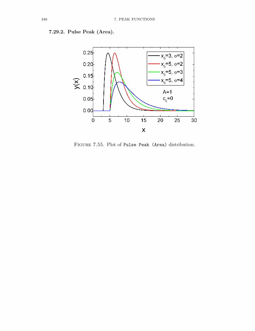
348 7. PEAK FUNCTIONS
7.29.2. Pulse Peak (Area).
Figure 7.55. Plot of Pulse Peak (Area) distribution.
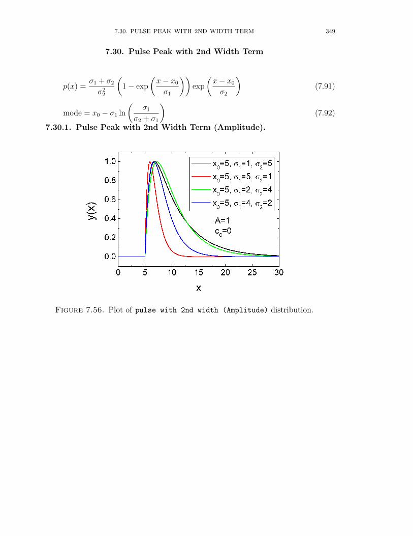
7.30. PULSE PEAK WITH 2ND WIDTH TERM 349
7.30. Pulse Peak with 2nd Width Term
p(x) =σ1 + σ2
σ22
(1− exp
(x− x0
σ1
))exp
(x− x0
σ2
)(7.91)
mode = x0 − σ1 ln
(σ1
σ2 + σ1
)(7.92)
7.30.1. Pulse Peak with 2nd Width Term (Amplitude).
Figure 7.56. Plot of pulse with 2nd width (Amplitude) distribution.
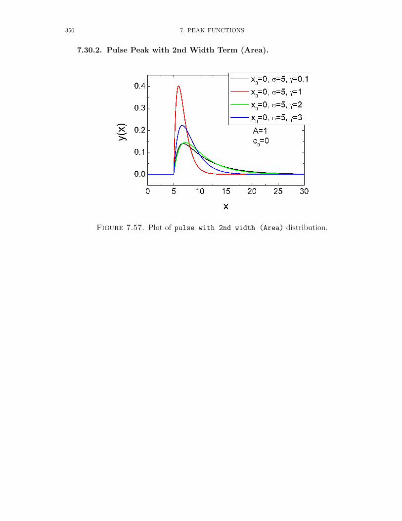
350 7. PEAK FUNCTIONS
7.30.2. Pulse Peak with 2nd Width Term (Area).
Figure 7.57. Plot of pulse with 2nd width (Area) distribution.
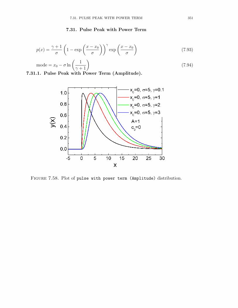
7.31. PULSE PEAK WITH POWER TERM 351
7.31. Pulse Peak with Power Term
p(x) =γ + 1
σ
(1− exp
(x− x0
σ
))γexp
(x− x0
σ
)(7.93)
mode = x0 − σ ln
(1
γ + 1
)(7.94)
7.31.1. Pulse Peak with Power Term (Amplitude).
Figure 7.58. Plot of pulse with power term (Amplitude) distribution.
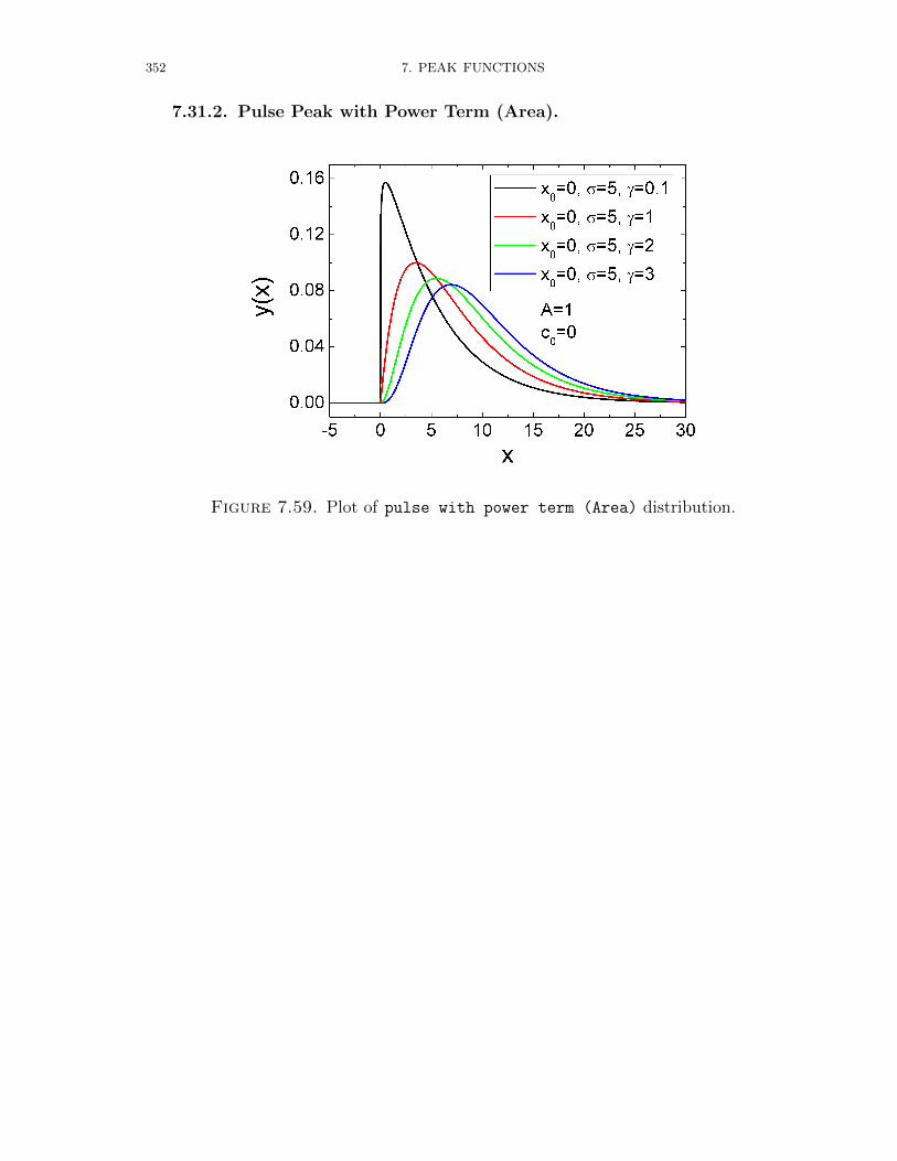
352 7. PEAK FUNCTIONS
7.31.2. Pulse Peak with Power Term (Area).
Figure 7.59. Plot of pulse with power term (Area) distribution.
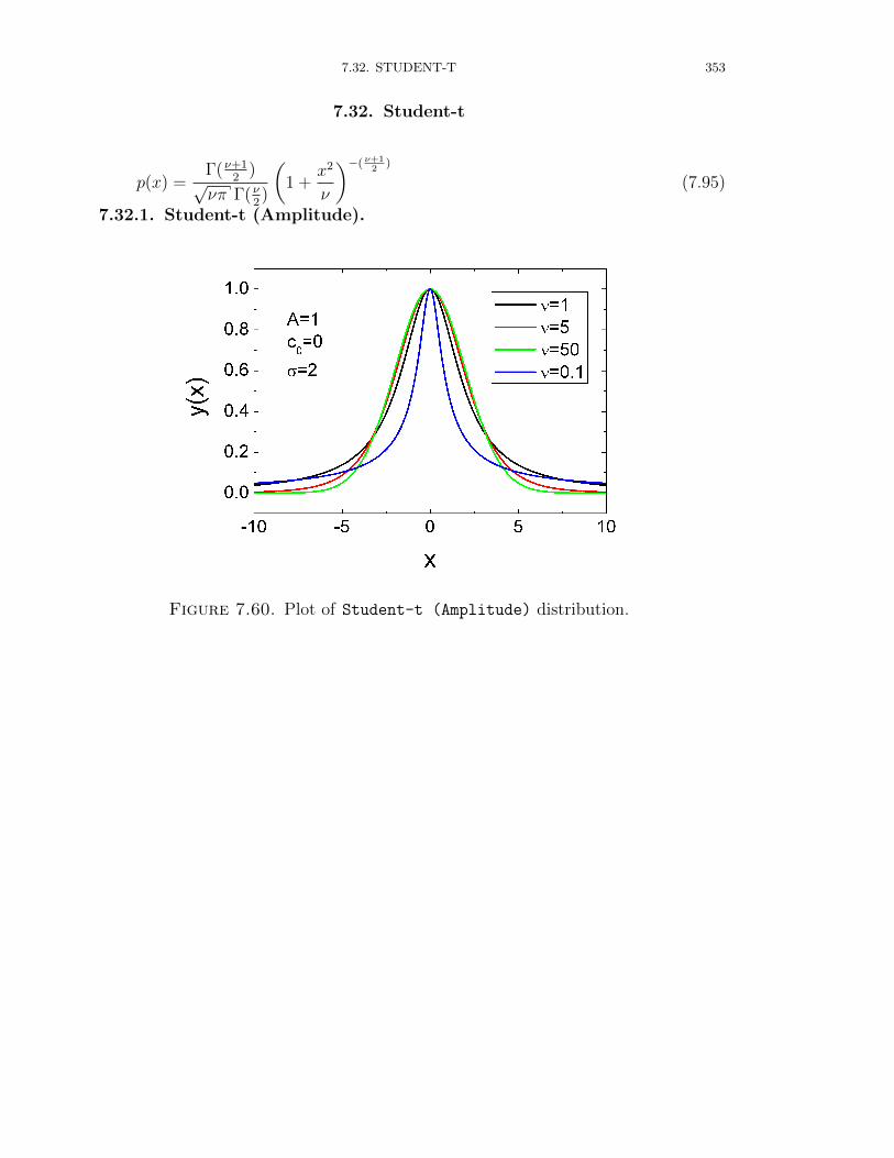
7.32. STUDENT-T 353
7.32. Student-t
p(x) =Γ(ν+1
2)
√νπ Γ(ν
2)
(1 +
x2
ν
)−( ν+12
)
(7.95)
7.32.1. Student-t (Amplitude).
Figure 7.60. Plot of Student-t (Amplitude) distribution.
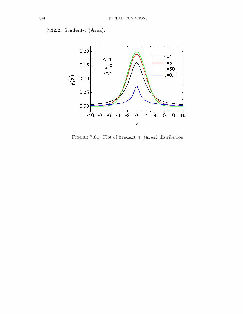
354 7. PEAK FUNCTIONS
7.32.2. Student-t (Area).
Figure 7.61. Plot of Student-t (Area) distribution.
7.33. VOIGT 355
7.33. Voigt
The Voigt profile is a spectral line profile found in all branches of spectroscopy in whicha spectral line is broadened by two types of mechanisms, one of which alone wouldproduce a Gaussian profile (usually, as a result of the Doppler broadening), and theother would produce a Lorentzian profile. The Voigt profile is then a convolution of aLorentz profile and a Gaussian profile:
V (x, xc|σ, γ) =
∞∫∞
D(x′|σ)L(x− xc − x′|γ) dx′ (7.96a)
where x− xc is distance from line center xc, D(x|σ) is the centered Doppler profile:
D(x|σ) =e−x
2/2σ2
σ√
2π(7.96b)
and L(x− xc|γ) is the centered Lorentzian profile:
L(x− xc|γ) =γ
π((x− xc)2 + γ2). (7.96c)
The defining integral can be evaluated as [29, 66]:
V (x, xc) =<[w(z)]
σ√
2π(7.96d)
where <[w(z)] is the real part of the complex error function of z and
z =x− xc + iγ
σ√
2(7.96e)
The full width at half maximum (FWHM) of the Voigt profile can be found from thewidths of the associated Gaussian and Lorentzian widths. The FWHM of the Gaussianprofile is fG = 2σ
√2 ln(2) . The FWHM of the Lorentzian profile is just fL = 2γ. Define
φ = fL/fG. Then the FWHM of the Voigt profile (fV) can be estimated as:
fV ≈ fG
(1− c0c1 +
√φ2 + 2c1φ+ c2
0c21
)(7.97)
where c0 = 2.0056 and c1 = 1.0593. This estimate will have a standard deviation of errorof about 2.4 percent for values of φ between 0 and 10. Note that the above equation willhave the proper behavior in the limit of φ = 0 and φ = ∞. A different approximationwas given by [104, 85]
fV ≈ 0.5346fL +√
0.2166f 2L + f 2
G (7.98)
with an accuracy of 0.02

356 7. PEAK FUNCTIONS
7.33.1. Voigt (Amplitude).
The amplitude version of the Voigt peak is parameterized as
VAmplitude(x|A, σ, γ) = A
∞∫−∞
exp(−u2)
γ2
2σ2 +(x−xc√
2 σ− u)2 du
∞∫−∞
exp(−u2)γ2
2σ2 + u2du
= AV (x, xc|σ, γ)
V (xc, xc|σ, γ)(7.99)
Required parameters:
ampl.: amplitude A of the Voigt peakcenter: location parameter (mode) xcsigma: width of Doppler (Gaussian) contribution σ > 0gamma: width of Lorentzian contribution γ > 0backgr: offset c0
Note
• The Doppler (Gaussian) width parameter needs to be larger than 0 σ > 0.• The Lorentzian width parameter needs to be larger than 0 γ > 0.• Default (Size) distribution: Monodisperse
Figure 7.62. Plot of Voigt (Area) distribution.
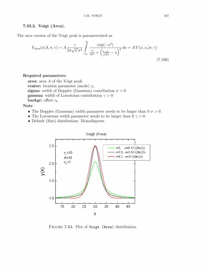
7.33. VOIGT 357
7.33.2. Voigt (Area).
The area version of the Voigt peak is parameterized as
VArea(x|A, σ, γ) = Aγ
2π√π σ2
∞∫−∞
exp(−u2)
γ2
2σ2 +(x−xc√
2 σ− u)2 du = AV (x, xc|σ, γ)
(7.100)
Required parameters:
area: area A of the Voigt peakcenter: location parameter (mode) xcsigma: width of Doppler (Gaussian) contribution σ > 0gamma: width of Lorentzian contribution γ > 0backgr: offset c0
Note
• The Doppler (Gaussian) width parameter needs to be larger than 0 σ > 0.• The Lorentzian width parameter needs to be larger than 0 γ > 0.• Default (Size) distribution: Monodisperse
Figure 7.63. Plot of Voigt (Area) distribution.
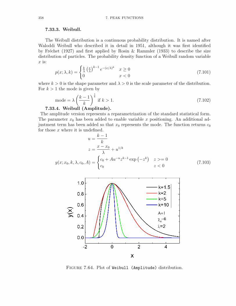
358 7. PEAK FUNCTIONS
7.33.3. Weibull.
The Weibull distribution is a continuous probability distribution. It is named afterWaloddi Weibull who described it in detail in 1951, although it was first identifiedby Frechet (1927) and first applied by Rosin & Rammler (1933) to describe the sizedistribution of particles. The probability density function of a Weibull random variablex is:
p(x;λ, k) =
kλ
(xλ
)k−1e−(x/λ)k x ≥ 0
0 x < 0(7.101)
where k > 0 is the shape parameter and λ > 0 is the scale parameter of the distribution.For k > 1 the mode is given by
mode = λ
(k − 1
k
) 1k
if k > 1. (7.102)
7.33.4. Weibull (Amplitude).The amplitude version represents a reparametrization of the standard statistical form.
The parameter x0 has been added to enable variable x positioning. An additional ad-justment term has been added so that x0 represents the mode. The function returns c0
for those x where it is undefined.
u =k − 1
k
z =x− x0
λ+ u1/k
y(x;x0, k, λ, c0, A) =
c0 + Au−uzk−1 exp
(−zk
)z >= 0
c0 z < 0(7.103)
Figure 7.64. Plot of Weibull (Amplitude) distribution.

7.33. VOIGT 359
7.33.5. Weibull (Area).The area version represents a reparametrization of the standard statistical form. The
parameter x0 has been added to enable variable x positioning. An additional adjustmentterm has been added so that x0 represents the mode. The function returns c0 for thosex where it is undefined.
z =x− x0
λ+
(k − 1
k
)1/k
y(x;x0, k, λ, c0, A) =
c0 + A k
λzk−1 exp
(−zk
)z >= 0
c0 z < 0(7.104)
Figure 7.65. Plot of Weibull (Area) distribution.

CHAPTER 8
Plugin functions
8.1. Very anisotropic particles (local planar & local cylindrical objects)
For very anisotropic random orientated particles the form factor can be factorizeaccording to Porod [117] in a cross section term Pcs(Q) for the shorter dimension and ashape factor P ′(Q) for the long dimension.
I(Q) = P ′(Q)Pcs(Q). (8.1)
In this plugin the form factors of two types of anisotropic particles are collected, thosewith a local cylindrical and with a local planar geometry. In case of local planar objectsthe cross section term Pcs(Q) can be homogeneous, a centro-symmetric bilayer, a gauss-ian bilayer, etc. . This cross section factor can than be combined with the overall shapefactor P ′(Q) of for examples a thin spherical shell of elliptical shell, a thin cylindricalshell or a thin disc. As the total form factor is the product of the cross-section formfactor and a shape form factor one can either programm all combination of cross-sectionand shape factors into individual form factor functions or one can programm the cross-section factors as form factor and the shape factor as a structure factors. Using themonodisperse approximation yields than the same result.
In this plugin the product of the cross-section and shape term have been imple-mented as form factor under ”[by plugin|anisotropic obj.|local planar obj.]”and ”[by plugin|anisotropic obj.|local cylindrical obj.]”. The cross-sectionterms alone are also implemented as form factors under ”[by plugin|anisotropic
obj.|Pcs(Q) for planar obj.]” and ”[by plugin|anisotropic obj.|Pcs(Q) for
cylindrical obj.]”. The shape factors are also available as structure fac-tors under ”[by plugin|anisotropic obj.|P’(Q): local planar obj.]” and ”[byplugin|anisotropic obj.|P’(Q): local cylindrical obj.]”.
The cross-section form factors can be easily calculated if the scattering length densitycontrast profile ∆ηcs(r) is known. For structures with a local planar geometry and asymmetric cross-section the form factor is given by
P planarcs (Q) =
2
∞∫0
∆ηcs(r) cos(Qr) dr
2
(8.2)
In case of local cylindrical particles with a centro-symmetric scattering length densitydistribution the form factor is given by
P cylindricalcs (Q) =
2π
∞∫0
∆ηcs(r)J0(Qr)r dr
2
(8.3)
361
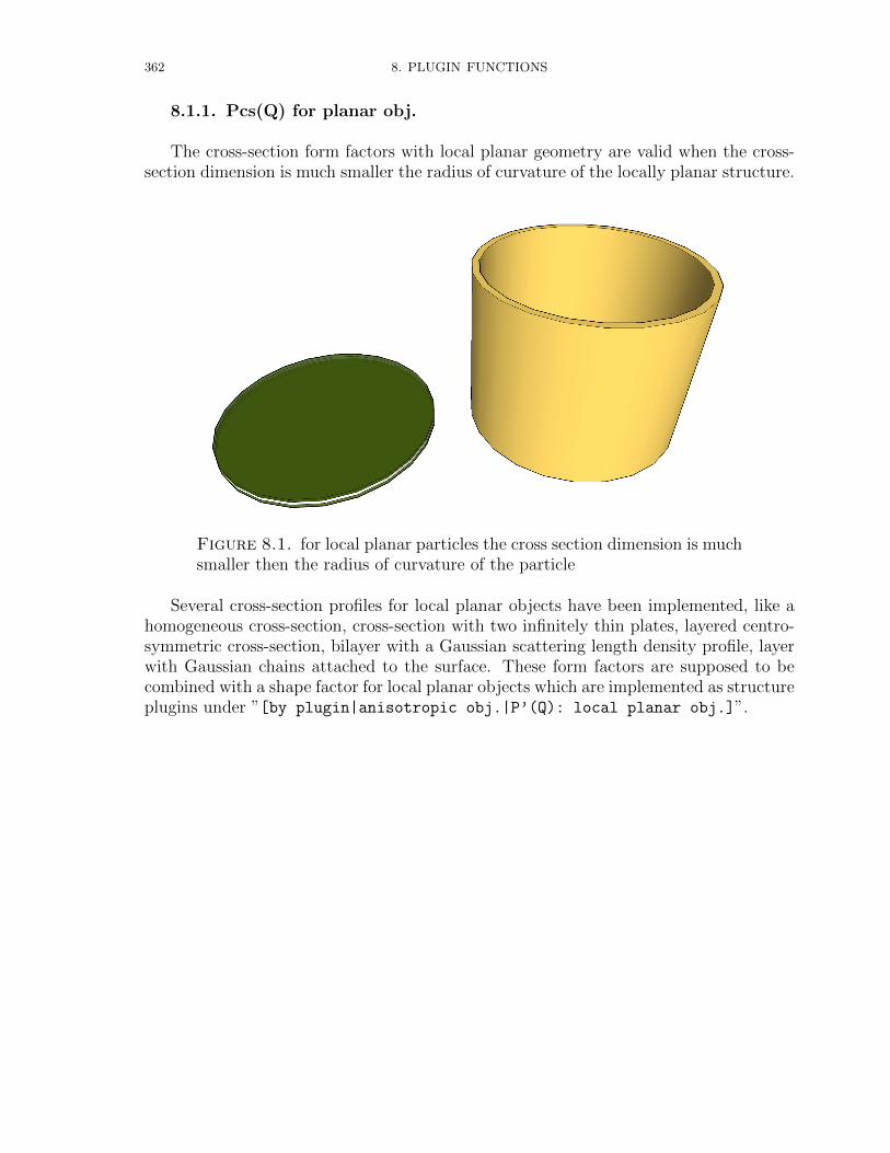
362 8. PLUGIN FUNCTIONS
8.1.1. Pcs(Q) for planar obj.
The cross-section form factors with local planar geometry are valid when the cross-section dimension is much smaller the radius of curvature of the locally planar structure.
Figure 8.1. for local planar particles the cross section dimension is muchsmaller then the radius of curvature of the particle
Several cross-section profiles for local planar objects have been implemented, like ahomogeneous cross-section, cross-section with two infinitely thin plates, layered centro-symmetric cross-section, bilayer with a Gaussian scattering length density profile, layerwith Gaussian chains attached to the surface. These form factors are supposed to becombined with a shape factor for local planar objects which are implemented as structureplugins under ”[by plugin|anisotropic obj.|P’(Q): local planar obj.]”.
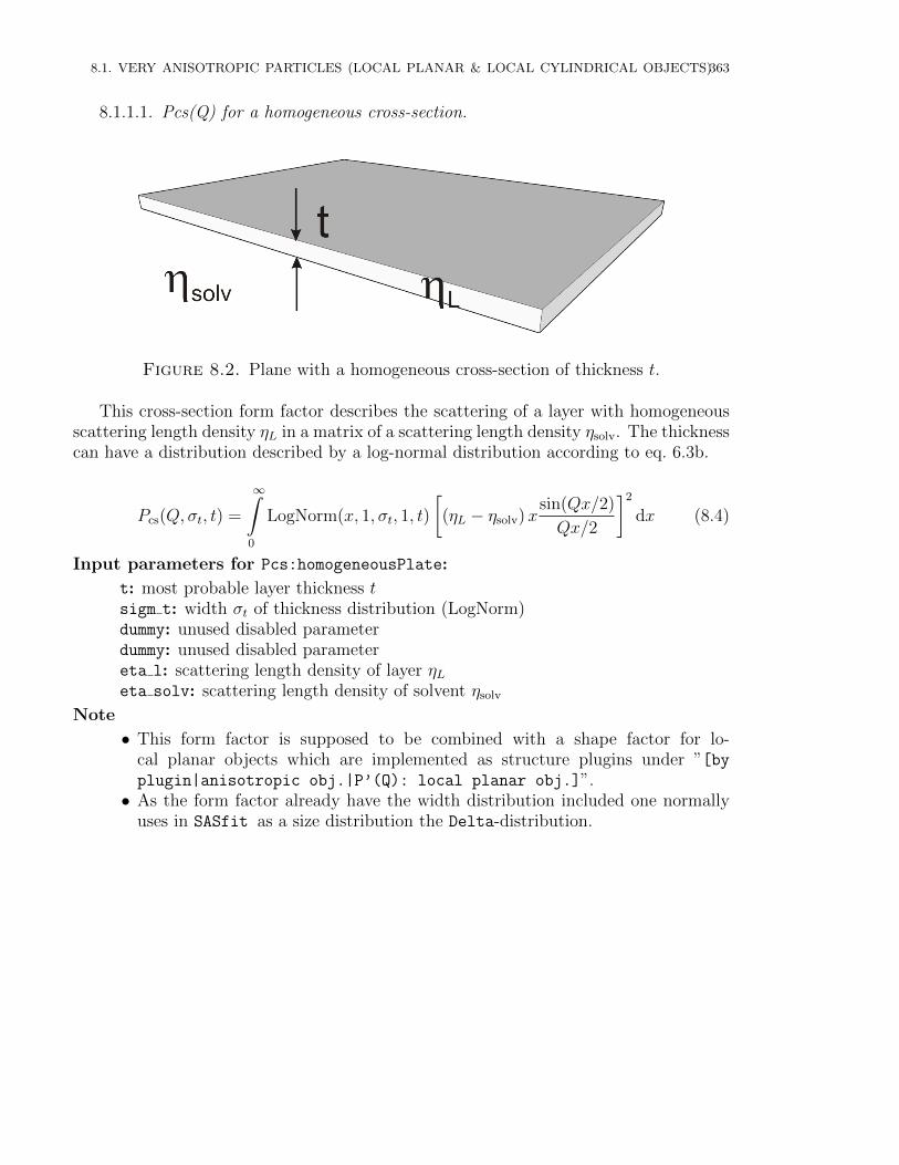
8.1. VERY ANISOTROPIC PARTICLES (LOCAL PLANAR & LOCAL CYLINDRICAL OBJECTS)363
8.1.1.1. Pcs(Q) for a homogeneous cross-section.
Figure 8.2. Plane with a homogeneous cross-section of thickness t.
This cross-section form factor describes the scattering of a layer with homogeneousscattering length density ηL in a matrix of a scattering length density ηsolv. The thicknesscan have a distribution described by a log-normal distribution according to eq. 6.3b.
Pcs(Q, σt, t) =
∞∫0
LogNorm(x, 1, σt, 1, t)
[(ηL − ηsolv)x
sin(Qx/2)
Qx/2
]2
dx (8.4)
Input parameters for Pcs:homogeneousPlate:
t: most probable layer thickness tsigm t: width σt of thickness distribution (LogNorm)dummy: unused disabled parameterdummy: unused disabled parametereta l: scattering length density of layer ηLeta solv: scattering length density of solvent ηsolv
Note
• This form factor is supposed to be combined with a shape factor for lo-cal planar objects which are implemented as structure plugins under ”[byplugin|anisotropic obj.|P’(Q): local planar obj.]”.• As the form factor already have the width distribution included one normally
uses in SASfit as a size distribution the Delta-distribution.

364 8. PLUGIN FUNCTIONS
Figure 8.3. Scattering curve for the form factor”Pcs:homogeneousPlate” only (insert) and in combination with astructure factor ”P’(Q): Thin Spherical Shell”.
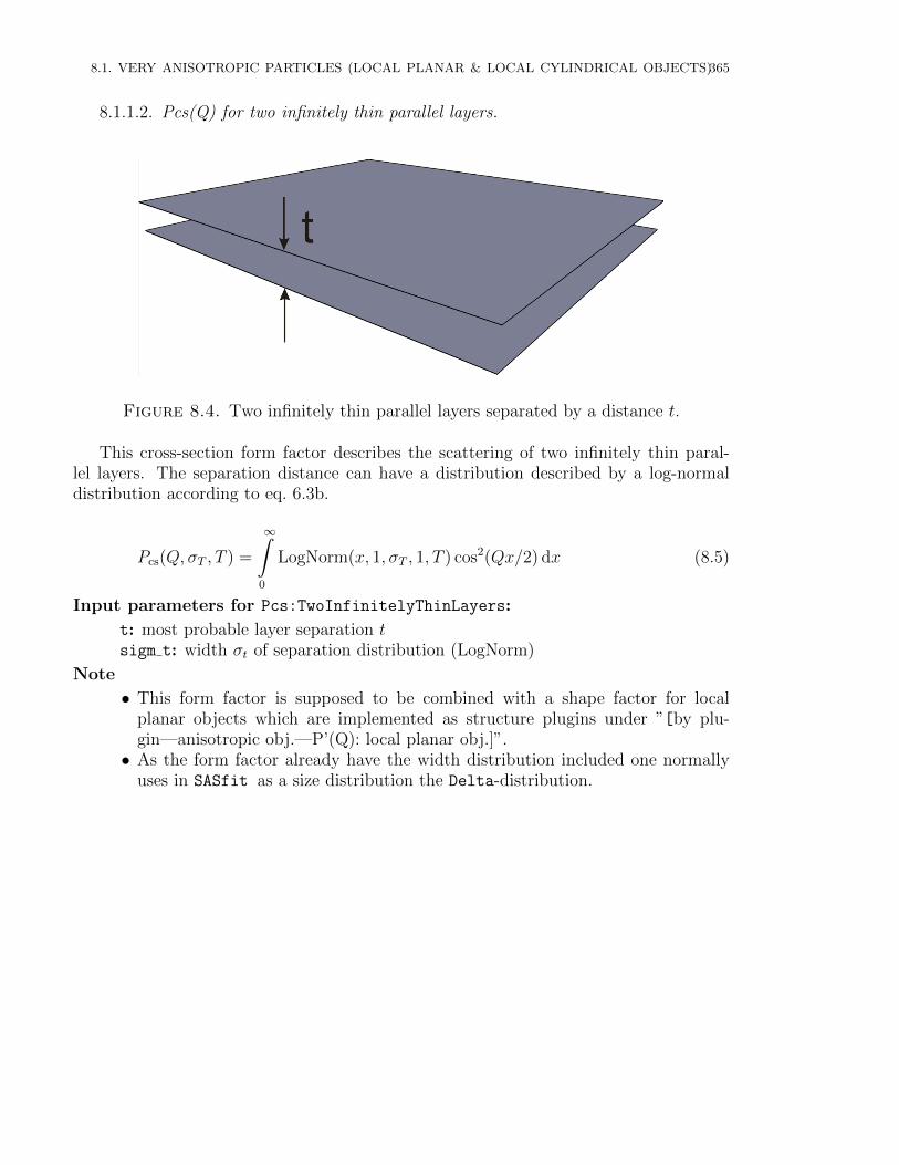
8.1. VERY ANISOTROPIC PARTICLES (LOCAL PLANAR & LOCAL CYLINDRICAL OBJECTS)365
8.1.1.2. Pcs(Q) for two infinitely thin parallel layers.
Figure 8.4. Two infinitely thin parallel layers separated by a distance t.
This cross-section form factor describes the scattering of two infinitely thin paral-lel layers. The separation distance can have a distribution described by a log-normaldistribution according to eq. 6.3b.
Pcs(Q, σT , T ) =
∞∫0
LogNorm(x, 1, σT , 1, T ) cos2(Qx/2) dx (8.5)
Input parameters for Pcs:TwoInfinitelyThinLayers:
t: most probable layer separation tsigm t: width σt of separation distribution (LogNorm)
Note
• This form factor is supposed to be combined with a shape factor for localplanar objects which are implemented as structure plugins under ”[by plu-gin—anisotropic obj.—P’(Q): local planar obj.]”.• As the form factor already have the width distribution included one normally
uses in SASfit as a size distribution the Delta-distribution.
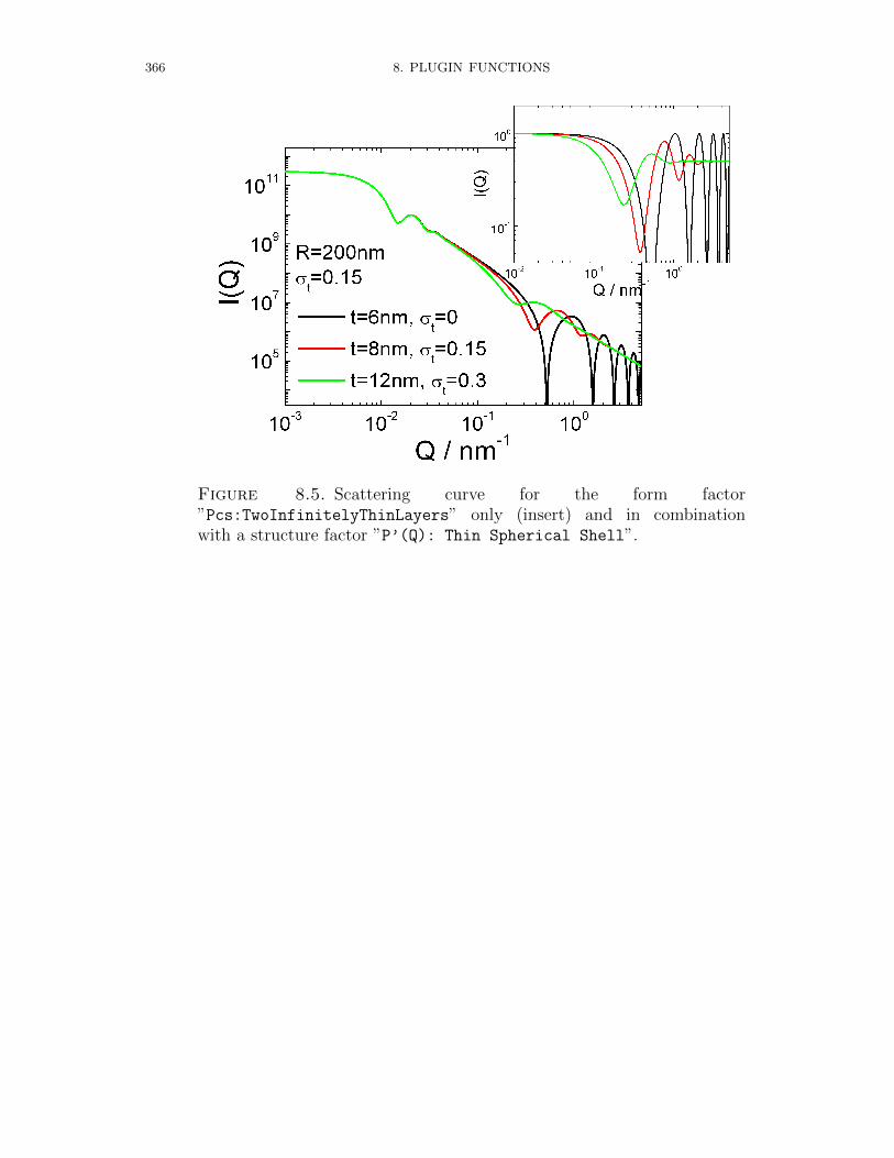
366 8. PLUGIN FUNCTIONS
Figure 8.5. Scattering curve for the form factor”Pcs:TwoInfinitelyThinLayers” only (insert) and in combinationwith a structure factor ”P’(Q): Thin Spherical Shell”.
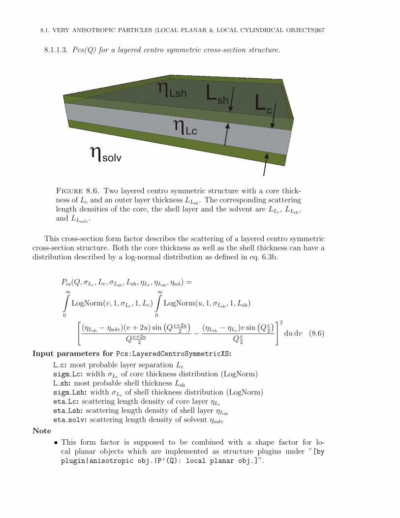
8.1. VERY ANISOTROPIC PARTICLES (LOCAL PLANAR & LOCAL CYLINDRICAL OBJECTS)367
8.1.1.3. Pcs(Q) for a layered centro symmetric cross-section structure.
Figure 8.6. Two layered centro symmetric structure with a core thick-ness of Lc and an outer layer thickness LLsh
. The corresponding scatteringlength densities of the core, the shell layer and the solvent are LLc , LLsh
,and LLsolv
.
This cross-section form factor describes the scattering of a layered centro symmetriccross-section structure. Both the core thickness as well as the shell thickness can have adistribution described by a log-normal distribution as defined in eq. 6.3b.
Pcs(Q, σLc , Lc, σLsh, Lsh, ηLc , ηLsh
, ηsol) =∞∫
0
LogNorm(v, 1, σLc , 1, Lc)
∞∫0
LogNorm(u, 1, σLsh, 1, Lsh)
[(ηLsh
− ηsolv)(v + 2u) sin(Qv+2u
2
)Qv+2u
2
−(ηLsh
− ηLc)v sin(Qv
2
)Qv
2
]2
du dv (8.6)
Input parameters for Pcs:LayeredCentroSymmetricXS:
L c: most probable layer separation Lc
sigm Lc: width σLc of core thickness distribution (LogNorm)L sh: most probable shell thickness Lsh
sigm Lsh: width σLc of shell thickness distribution (LogNorm)eta Lc: scattering length density of core layer ηLc
eta Lsh: scattering length density of shell layer ηLsh
eta solv: scattering length density of solvent ηsolv
Note
• This form factor is supposed to be combined with a shape factor for lo-cal planar objects which are implemented as structure plugins under ”[byplugin|anisotropic obj.|P’(Q): local planar obj.]”.
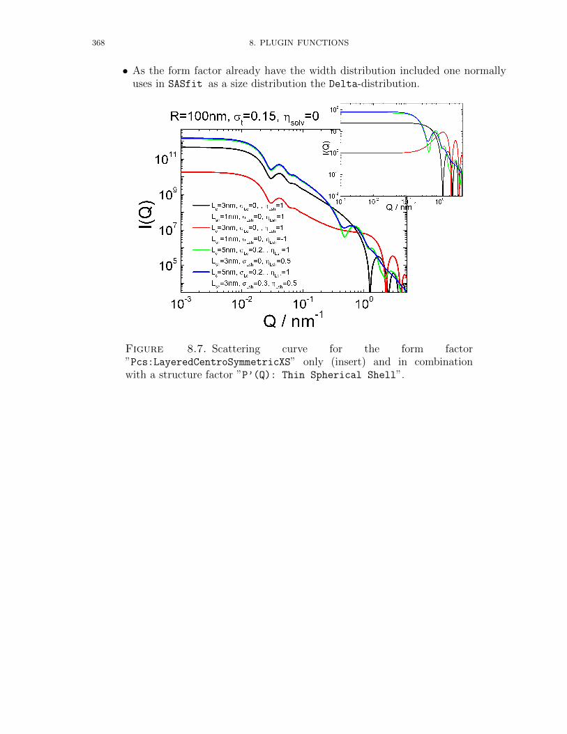
368 8. PLUGIN FUNCTIONS
• As the form factor already have the width distribution included one normallyuses in SASfit as a size distribution the Delta-distribution.
Figure 8.7. Scattering curve for the form factor”Pcs:LayeredCentroSymmetricXS” only (insert) and in combinationwith a structure factor ”P’(Q): Thin Spherical Shell”.
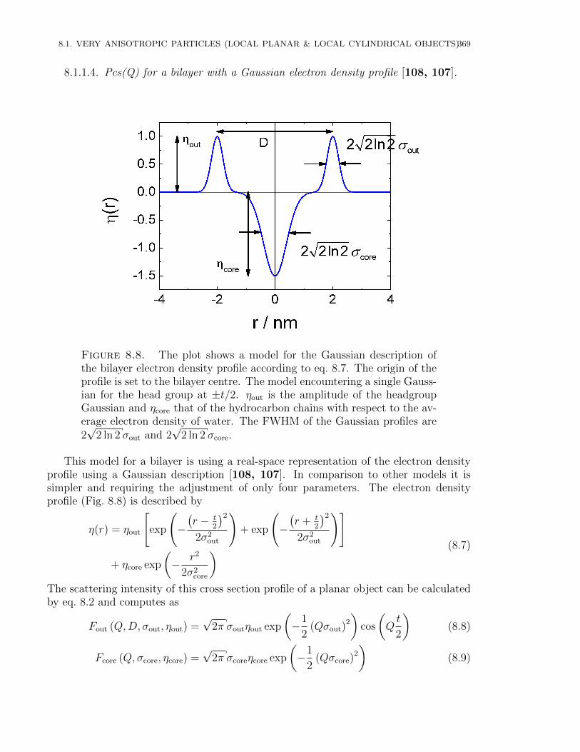
8.1. VERY ANISOTROPIC PARTICLES (LOCAL PLANAR & LOCAL CYLINDRICAL OBJECTS)369
8.1.1.4. Pcs(Q) for a bilayer with a Gaussian electron density profile [108, 107].
Figure 8.8. The plot shows a model for the Gaussian description ofthe bilayer electron density profile according to eq. 8.7. The origin of theprofile is set to the bilayer centre. The model encountering a single Gauss-ian for the head group at ±t/2. ηout is the amplitude of the headgroupGaussian and ηcore that of the hydrocarbon chains with respect to the av-erage electron density of water. The FWHM of the Gaussian profiles are2√
2 ln 2 σout and 2√
2 ln 2 σcore.
This model for a bilayer is using a real-space representation of the electron densityprofile using a Gaussian description [108, 107]. In comparison to other models it issimpler and requiring the adjustment of only four parameters. The electron densityprofile (Fig. 8.8) is described by
η(r) = ηout
[exp
(−(r − t
2
)2
2σ2out
)+ exp
(−(r + t
2
)2
2σ2out
)]
+ ηcore exp
(− r2
2σ2core
) (8.7)
The scattering intensity of this cross section profile of a planar object can be calculatedby eq. 8.2 and computes as
Fout (Q,D, σout, ηout) =√
2π σoutηout exp
(−1
2(Qσout)
2
)cos
(Qt
2
)(8.8)
Fcore (Q, σcore, ηcore) =√
2π σcoreηcore exp
(−1
2(Qσcore)
2
)(8.9)

370 8. PLUGIN FUNCTIONS
so that
Pcs (Q) = [Fcore (Q, σcore, ηcore) + 2Fout (Q,D, σout, ηout)]2 (8.10)
Input parameters for Pcs:BilayerGauss:
sigma core: width σout of the central Gaussian profileeta core: scattering length density contrast of the central Gaussian profilesigma out: width σout of the two outer Gaussian profileseta out: scattering length density contrast of the two outer Gaussian profilest: distance between the centers of the outer Gaussian profiles
Note
• This form factor is supposed to be combined with a shape factor for lo-cal planar objects which are implemented as structure plugins under ”[byplugin|anisotropic obj.|P’(Q): local planar obj.]”.
(a) Plot of the cross section form factor Pcs incombination with a structure factor ”P’(Q):Thin Disc” as the shape factor P ′(Q).
(b) Plot of the cross section form factor Pcs
only according to eq. 8.10. The parametersfor the profile are the same than in Fig. 8.9a
Figure 8.9. Scattering curve for the cross-section form factor”Pcs:BilayerGaussian”. For some of the curves a distance distribu-tion of the heads groups are assumed being Gaussian (see eq. 6.22a), i.e.calculating
∫∞0
Gauss(D, 1, σGaussD , D0)Pcs (Q,D) dD.
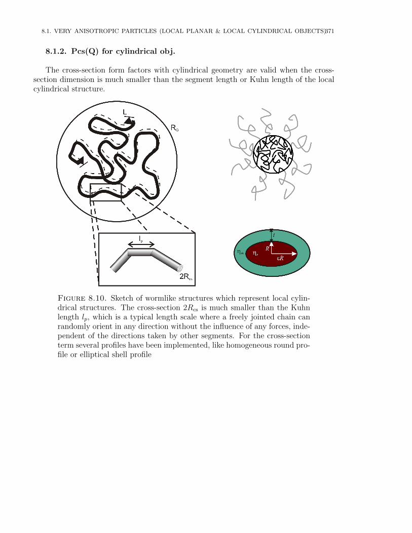
8.1. VERY ANISOTROPIC PARTICLES (LOCAL PLANAR & LOCAL CYLINDRICAL OBJECTS)371
8.1.2. Pcs(Q) for cylindrical obj.
The cross-section form factors with cylindrical geometry are valid when the cross-section dimension is much smaller than the segment length or Kuhn length of the localcylindrical structure.
Figure 8.10. Sketch of wormlike structures which represent local cylin-drical structures. The cross-section 2Rcs is much smaller than the Kuhnlength lp, which is a typical length scale where a freely jointed chain canrandomly orient in any direction without the influence of any forces, inde-pendent of the directions taken by other segments. For the cross-sectionterm several profiles have been implemented, like homogeneous round pro-file or elliptical shell profile
372 8. PLUGIN FUNCTIONS
8.1.2.1. Pcs(Q) for homogeneous cross-section of a cylinder.
This cross-section form factor describes the scattering of circular and homogeneouscross section. The cross-section radius R can have a distribution described by a log-normal distribution according to eq. 6.3b.
Pcs(Q, σR, R) =
∞∫0
LogNorm(x, 1, σR, 1, R)
((ηcore − ηsolv) πx2 2J1(Qx)
Qx
)2
dx
(8.11)
Input parameters for Pcs:homogeneousCyl:
R: most probable radius Rsigm R: width σR of radius distribution (LogNorm)dummy: not useddummy: not useddummy: not useddummy: not useddummy: not usedeta core: scattering length density of the core ηcore
dummy: not usedeta solv: scattering length density of the solvent ηsolv
Note
• This form factor is supposed to be combined with a shape factor for localcylindrical objects which are implemented as structure plugins under ”[byplugin|anisotropic obj.|P’(Q): local cylindrical obj.]”.• As the form factor already have the width distribution included one normally
uses in SASfit as a size distribution the Delta-distribution.

8.1. VERY ANISOTROPIC PARTICLES (LOCAL PLANAR & LOCAL CYLINDRICAL OBJECTS)373
Figure 8.11. Scattering curve for the form factor”Pcs:homogeneousCyl” only (insert) and in combination with astructure factor ”P’(Q): Thin Rod”.
374 8. PLUGIN FUNCTIONS
8.1.2.2. Pcs(Q) for cross-section of a cylindrical shell with elliptical cross section.
This cross-section form factor describes the scattering of an elliptical core-shell cross-section. The cross-section radius R can have a distribution with a width of sigma asdescribed by a log-normal distribution according to eq. 6.3b.
Pcs(Q) =
∞∫0
LogNorm(x, 1, σR, 1, R) ×
π/2∫0
[(ηshell − ηsolv)Fcs,ell(Q,R + t, ε, φ)
+ (ηcore − ηshell)Fcs,ell(Q,R, ε, φ)]2
dφ
(8.12)
with
Fcs,ell (Q,R, ε,∆ηφ) =2J1(Qr(R, ε, φ))
Qr(R, ε, φ)(8.13a)
r(R, ε, φ) = R
√sin2 φ+ ε2 cos2 φ (8.13b)
Input parameters for Pcs:homogeneousCyl:
R: most probable radius Rsigm R: width σR of radius distribution (LogNorm)epsilon: eccentricity ε of ellipyical cross-sectiont: shell thickness tdummy: not useddummy: not useddummy: not usedeta core: scattering length density of the core ηcore
eta shell: scattering length density of the shell ηshell
eta solv: scattering length density of the solvent ηsolv
Note
• This form factor is supposed to be combined with a shape factor for localcylindrical objects which are implemented as structure plugins under ”[byplugin|anisotropic obj.|P’(Q): local cylindrical obj.]”.• As the form factor already has the width distribution included one normally
uses in SASfit as a size distribution the Delta-distribution.
8.1. VERY ANISOTROPIC PARTICLES (LOCAL PLANAR & LOCAL CYLINDRICAL OBJECTS)375
8.1.3. P’(Q) for local planar obj.

376 8. PLUGIN FUNCTIONS
8.1.3.1. P’(Q): thin discs.
Figure 8.12. Sketch of a thin disc with a radius R. The thickness of thedisc is assumed to be much smaller than its radius.
Input parameters for P’(Q): Thin Disc:
R: most probable radius Rdummy: not usedsima: width σ of radius distribution (LogNorm)
Note
• This structure factor is supposed to be combined with a form factor of lo-cal planar objects which are implemented as form factor plugins under ”[byplugin|anisotropic obj.|Pcs(Q): local planar obj.]”.• The structure factor already has a log-normal width distribution for one pa-
rameter included.
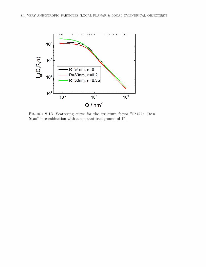
8.1. VERY ANISOTROPIC PARTICLES (LOCAL PLANAR & LOCAL CYLINDRICAL OBJECTS)377
Figure 8.13. Scattering curve for the structure factor ”P’(Q): Thin
Disc” in combination with a constant background of 1”.
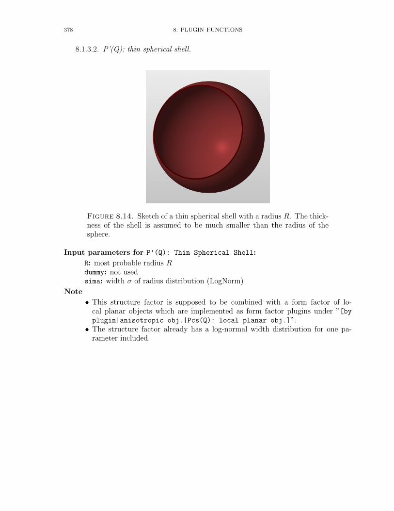
378 8. PLUGIN FUNCTIONS
8.1.3.2. P’(Q): thin spherical shell.
Figure 8.14. Sketch of a thin spherical shell with a radius R. The thick-ness of the shell is assumed to be much smaller than the radius of thesphere.
Input parameters for P’(Q): Thin Spherical Shell:
R: most probable radius Rdummy: not usedsima: width σ of radius distribution (LogNorm)
Note
• This structure factor is supposed to be combined with a form factor of lo-cal planar objects which are implemented as form factor plugins under ”[byplugin|anisotropic obj.|Pcs(Q): local planar obj.]”.• The structure factor already has a log-normal width distribution for one pa-
rameter included.
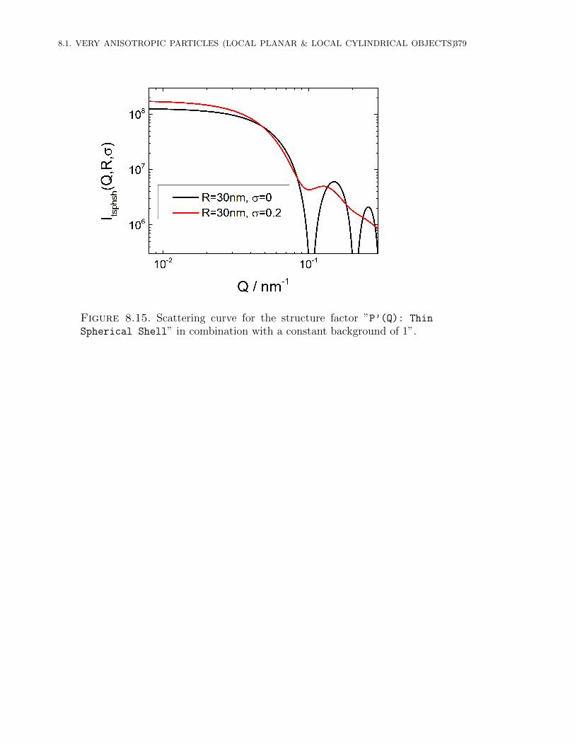
8.1. VERY ANISOTROPIC PARTICLES (LOCAL PLANAR & LOCAL CYLINDRICAL OBJECTS)379
Figure 8.15. Scattering curve for the structure factor ”P’(Q): Thin
Spherical Shell” in combination with a constant background of 1”.
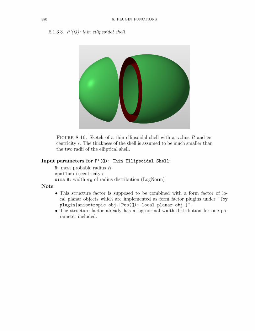
380 8. PLUGIN FUNCTIONS
8.1.3.3. P’(Q): thin ellipsoidal shell.
Figure 8.16. Sketch of a thin ellipsoidal shell with a radius R and ec-centricity ε. The thickness of the shell is assumed to be much smaller thanthe two radii of the elliptical shell.
Input parameters for P’(Q): Thin Ellipsoidal Shell:
R: most probable radius Repsilon: eccentricity εsima R: width σR of radius distribution (LogNorm)
Note
• This structure factor is supposed to be combined with a form factor of lo-cal planar objects which are implemented as form factor plugins under ”[byplugin|anisotropic obj.|Pcs(Q): local planar obj.]”.• The structure factor already has a log-normal width distribution for one pa-
rameter included.
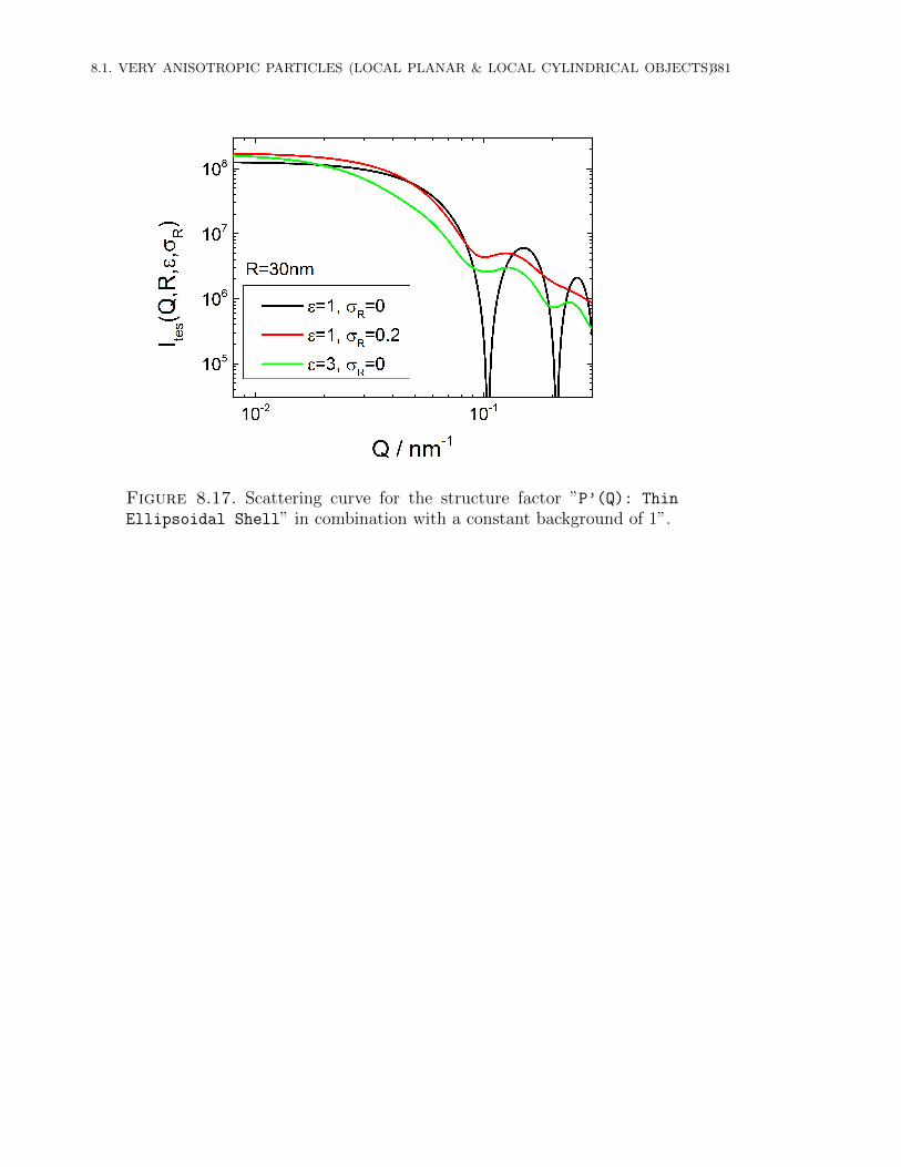
8.1. VERY ANISOTROPIC PARTICLES (LOCAL PLANAR & LOCAL CYLINDRICAL OBJECTS)381
Figure 8.17. Scattering curve for the structure factor ”P’(Q): Thin
Ellipsoidal Shell” in combination with a constant background of 1”.
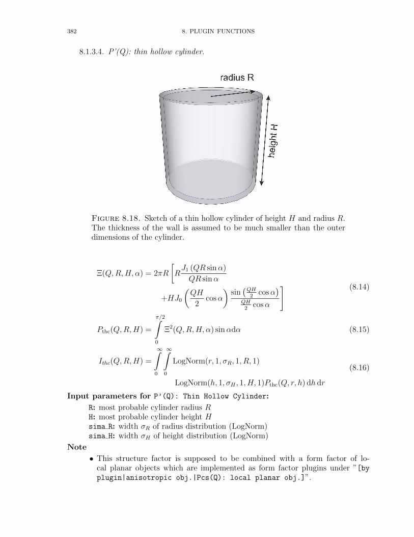
382 8. PLUGIN FUNCTIONS
8.1.3.4. P’(Q): thin hollow cylinder.
Figure 8.18. Sketch of a thin hollow cylinder of height H and radius R.The thickness of the wall is assumed to be much smaller than the outerdimensions of the cylinder.
Ξ(Q,R,H, α) = 2πR
[RJ1 (QR sinα)
QR sinα
+HJ0
(QH
2cosα
)sin(QH
2cosα
)QH
2cosα
] (8.14)
Pthc(Q,R,H) =
π/2∫0
Ξ2(Q,R,H, α) sinαdα (8.15)
Ithc(Q,R,H) =
∞∫0
∞∫0
LogNorm(r, 1, σR, 1, R, 1)
LogNorm(h, 1, σH , 1, H, 1)Pthc(Q, r, h) dh dr
(8.16)
Input parameters for P’(Q): Thin Hollow Cylinder:
R: most probable cylinder radius RH: most probable cylinder height Hsima R: width σR of radius distribution (LogNorm)sima H: width σH of height distribution (LogNorm)
Note
• This structure factor is supposed to be combined with a form factor of lo-cal planar objects which are implemented as form factor plugins under ”[byplugin|anisotropic obj.|Pcs(Q): local planar obj.]”.
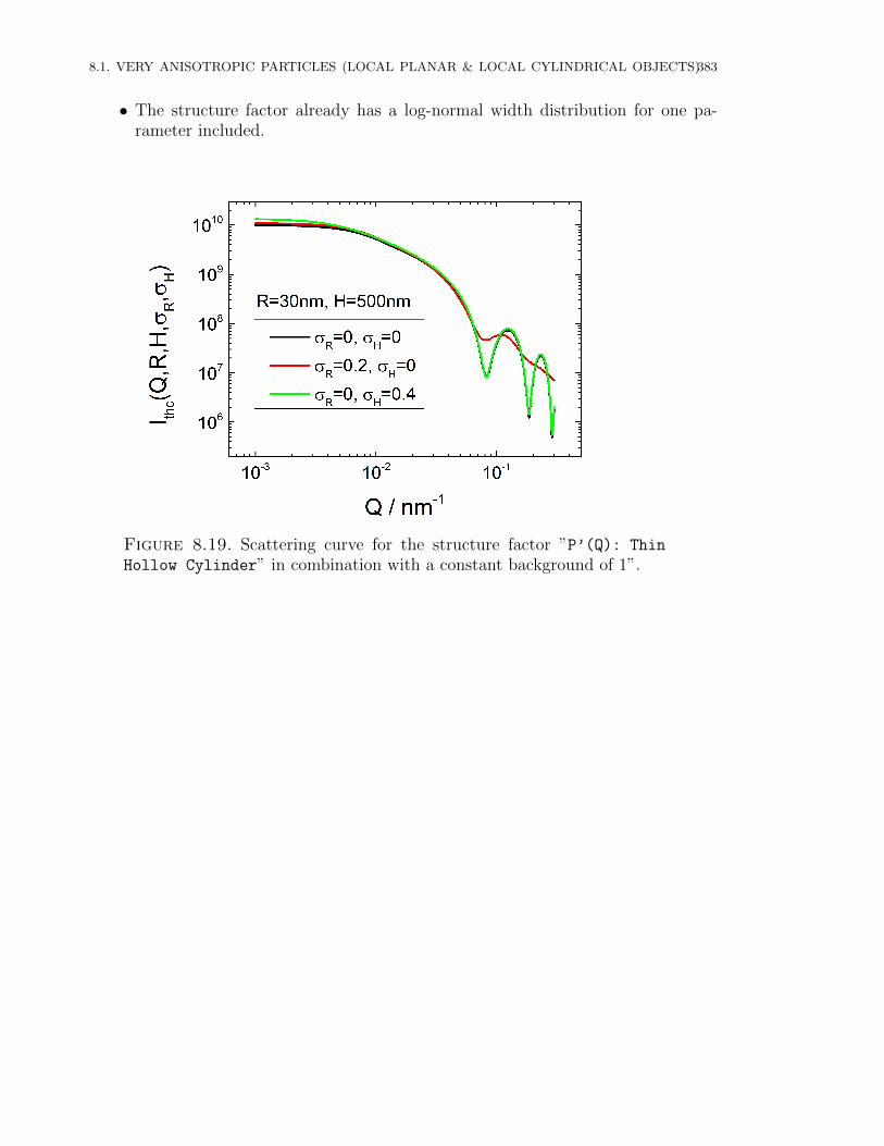
8.1. VERY ANISOTROPIC PARTICLES (LOCAL PLANAR & LOCAL CYLINDRICAL OBJECTS)383
• The structure factor already has a log-normal width distribution for one pa-rameter included.
Figure 8.19. Scattering curve for the structure factor ”P’(Q): Thin
Hollow Cylinder” in combination with a constant background of 1”.

384 8. PLUGIN FUNCTIONS
8.1.4. P’(Q) for local cylindrical obj.
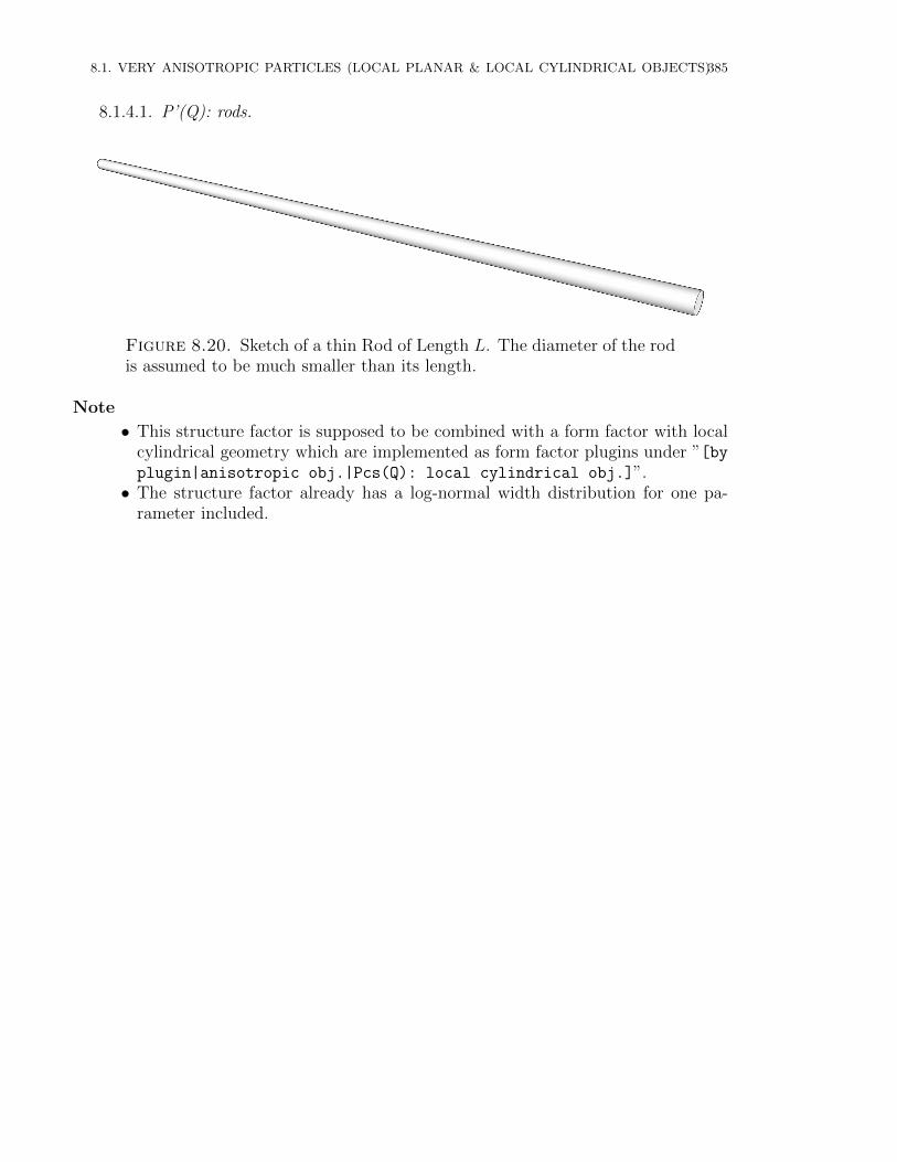
8.1. VERY ANISOTROPIC PARTICLES (LOCAL PLANAR & LOCAL CYLINDRICAL OBJECTS)385
8.1.4.1. P’(Q): rods.
Figure 8.20. Sketch of a thin Rod of Length L. The diameter of the rodis assumed to be much smaller than its length.
Note
• This structure factor is supposed to be combined with a form factor with localcylindrical geometry which are implemented as form factor plugins under ”[byplugin|anisotropic obj.|Pcs(Q): local cylindrical obj.]”.• The structure factor already has a log-normal width distribution for one pa-
rameter included.
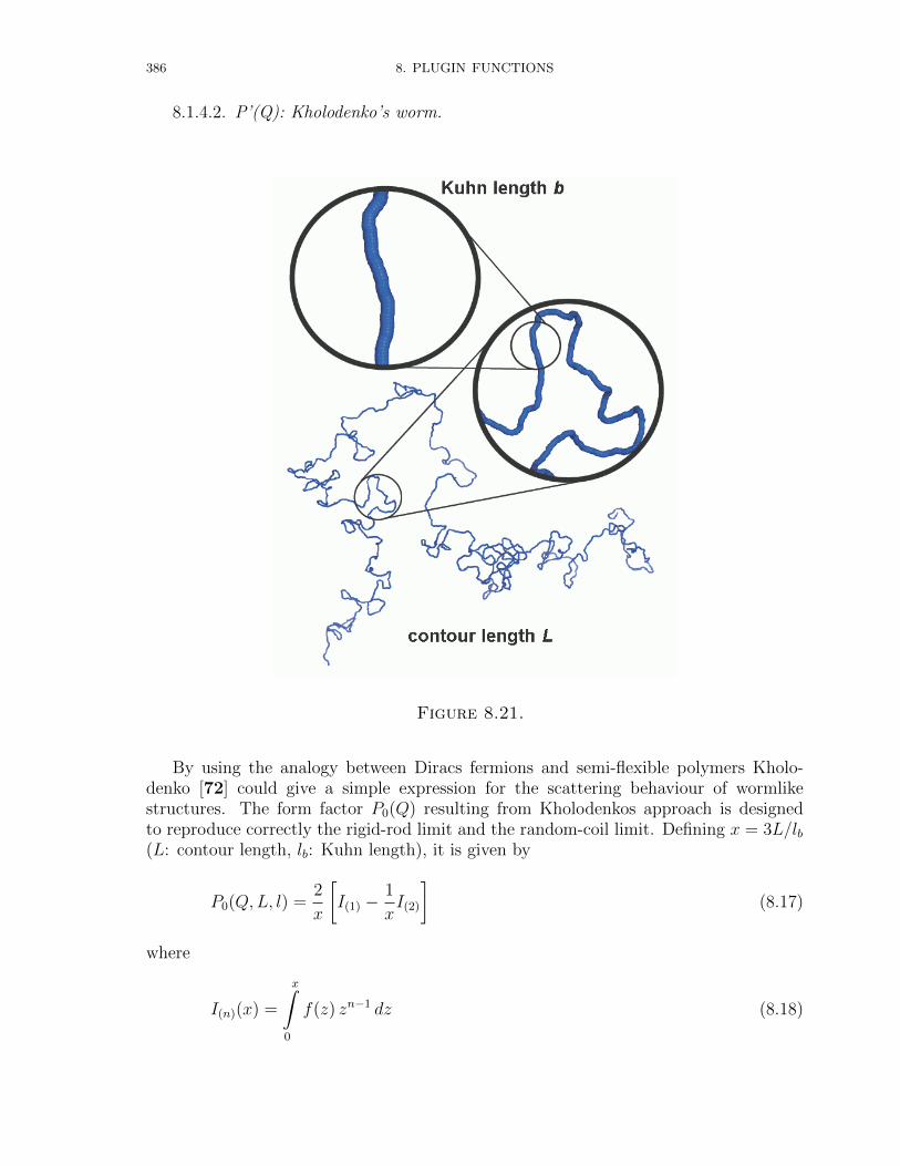
386 8. PLUGIN FUNCTIONS
8.1.4.2. P’(Q): Kholodenko’s worm.
Figure 8.21.
By using the analogy between Diracs fermions and semi-flexible polymers Kholo-denko [72] could give a simple expression for the scattering behaviour of wormlikestructures. The form factor P0(Q) resulting from Kholodenkos approach is designedto reproduce correctly the rigid-rod limit and the random-coil limit. Defining x = 3L/lb(L: contour length, lb: Kuhn length), it is given by
P0(Q,L, l) =2
x
[I(1) −
1
xI(2)
](8.17)
where
I(n)(x) =
x∫0
f(z) zn−1 dz (8.18)
8.1. VERY ANISOTROPIC PARTICLES (LOCAL PLANAR & LOCAL CYLINDRICAL OBJECTS)387
together with
f(z)) =
1
E
sinh(Ez)
sinh(z)for Q ≤ 3
l
1
F
sin(Fz)
sinh(z)for Q >
3
l
(8.19)
and
E =
√1−
(lQ
3
)2
and F =
√(lQ
3
)2
− 1 (8.20)
P (Q,L, lb, R) = P0(Q,L, lb)Pcs(Q,R) (8.21)
Input Parameters for model P’(Q) Kholodenko Worm:
lb: Kuhn length1 l of semi-flexible worm-like structureL: contour length L of semi-flexible worm-like structure
Note
• This structure factor is supposed to be combined with a form factor with localcylindrical geometry which are implemented as form factor plugins under ”[byplugin|anisotropic obj.|Pcs(Q): local cylindrical obj.]”.• The structure factor already has a log-normal width distribution for one pa-
rameter included.• The equivalent solution of J.S. Pedersen [110] would be the expressions of worm-
like structures without excluded volume effects.
1The Kuhn length lb is related to the length a of locally stiff segment simply via lb = 2a
388 8. PLUGIN FUNCTIONS
8.1.4.3. P’(Q): wormlike PS1.
For worm-like micelles J.S. Pedersen [110] has developed three models for worm-likemicelles, from which one is basing on a method developed by Yoshizaki et al. [155].
Without Excluded Volume Effects. This first of the three solutions given byJ.S. Pedersen [110] for worm-like micelles starts from the expression for the scatteringfunction as follows:
SWC(Q,L, lB) = L2 [(1− χ(Q,L, lB))Schain(Q,L, lB)
+χ(Q,L, lB)Srod(Q,L)] Γ(Q,L, lB)(8.22)
where Schain(Q,L, lB) is the scattering function of a flexible chain without excludedvolume effects and Srod(Q,L) is the scattering function of a rod. Furthermore, χ(Q,L, lb)is a crossover function, and the function Γ(q, L, b) corrects the crossover region. Thefunction Schain(Q,L, lB) is given by the Debye function:
Schain(Q,L, lB) = SDebye(Q,L, lB) = 2 [exp(−u) + u− 1] /u2 (8.23)
with u =⟨R2g
⟩0Q2, where
⟨R2g
⟩0
is the ensemble average of the square of the radius ofgyration and given by⟨
R2g
⟩0
=LlB6
[1− 3
2nB+
3
2n2B
− 3
4n3B
[1− exp(−2nB)]
](8.24)
where nB = L/lB b is the number of statistical segments of the chain. The functionSrod(Q,L) in 8.22 is the scattering function of an infinitely thin rod
Srod(Q,L) = 2Si(Q,L)/(QL)− 4 sin2(QL/2)/(QL)2 (8.25)
where
Si(Q,L) =
x∫0
t−1 sin t dt (8.26)
Furthermore we have
χ(Q,L, lB) = exp(−ξ−5
)(8.27)
The parameter ξ is given by
ξ = Qπ
2L
⟨R2g
⟩0
(8.28)
The function Γ(Q,L, lB) is given by
Γ(Q,L, lB) = 1 + (1− χ)5∑i=2
Aiξi + χ
2∑i=0
Biξ−i (8.29)
where
Ai =2∑j=0
a1(i, j)
(L
lB
)−jexp(−10lB/L)
+2∑j=1
a2(i, j)
(L
lB
)jexp(−2L/lB)
(8.30)
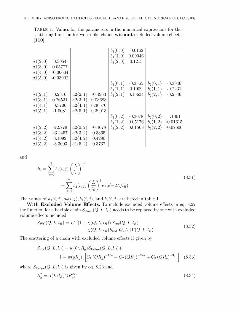
8.1. VERY ANISOTROPIC PARTICLES (LOCAL PLANAR & LOCAL CYLINDRICAL OBJECTS)389
Table 1. Values for the parameters in the numerical expressions for thescattering function for worm-like chains without excluded volume effects[110]
b1(0, 0) -0.0162b1(1, 0) 0.09046
a1(2, 0) 0.3054 b1(2, 0) 0.1213a1(3, 0) 0.05777a1(4, 0) -0.00604a1(5, 0) -0.03902
b1(0, 1) -0.3565 b2(0, 1) -0.3946b1(1, 1) 0.1909 b2(1, 1) -0.2231
a1(2, 1) 0.2316 a2(2, 1) -0.4963 b1(2, 1) 0.15634 b2(2, 1) -0.2546a1(3, 1) 0.26531 a2(3, 1) 0.03688a1(4, 1) 0.3706 a2(4, 1) 0.30570a1(5, 1) -1.0081 a2(5, 1) 0.39013
b1(0, 2) -0.3078 b2(0, 2) 1.1361b1(1, 2) 0.05176 b2(1, 2) -0.01615
a1(2, 2) -22.779 a2(2, 2) -0.4678 b1(2, 2) 0.01568 b2(2, 2) -0.07606a1(3, 2) 23.2457 a2(3, 2) 0.3365a1(4, 2) 8.1092 a2(4, 2) 0.4290a1(5, 2) -3.3603 a1(5, 2) 0.3737
and
Bi =2∑j=0
b1(i, j)
(L
lB
)−j
+2∑j=1
b2(i, j)
(L
lB
)jexp(−2L/lB)
(8.31)
The values of a1(i, j), a2(i, j), b1(i, j), and b2(i, j) are listed in table 1With Excluded Volume Effects. To include excluded volume effects in eq. 8.22
the function for a flexible chain Schain(Q,L, lB) needs to be replaced by one with excludedvolume effects included
SWC(Q,L, lB) = L2 [(1− χ(Q,L, lB))Sexv(Q,L, lB)
+χ(Q,L, lB)Srod(Q,L)] Γ(Q,L, lB)(8.32)
The scattering of a chain with excluded volume effects if given by
Sexv(Q,L, lB) = w(Q,Rg)SDebye(Q,L, lB)+
[1− w(qRg)[[C1 (QRg)
−1/ν + C2 (QRg)−2/ν + C3 (QRg)
−3/ν]
(8.33)
where SDebye(Q,L, lB) is given by eq. 8.23 and
R2g = α(L/lB)2〈R2
g〉2 (8.34)
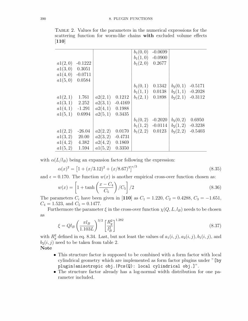
390 8. PLUGIN FUNCTIONS
Table 2. Values for the parameters in the numerical expressions for thescattering function for worm-like chains with excluded volume effects[110]
b1(0, 0) -0.0699b1(1, 0) -0.0900
a1(2, 0) -0.1222 b1(2, 0) 0.2677a1(3, 0) 0.3051a1(4, 0) -0.0711a1(5, 0) 0.0584
b1(0, 1) 0.1342 b2(0, 1) -0.5171b1(1, 1) 0.0138 b2(1, 1) -0.2028
a1(2, 1) 1.761 a2(2, 1) 0.1212 b1(2, 1) 0.1898 b2(2, 1) -0.3112a1(3, 1) 2.252 a2(3, 1) -0.4169a1(4, 1) -1.291 a2(4, 1) 0.1988a1(5, 1) 0.6994 a2(5, 1) 0.3435
b1(0, 2) -0.2020 b2(0, 2) 0.6950b1(1, 2) -0.0114 b2(1, 2) -0.3238
a1(2, 2) -26.04 a2(2, 2) 0.0170 b1(2, 2) 0.0123 b2(2, 2) -0.5403a1(3, 2) 20.00 a2(3, 2) -0.4731a1(4, 2) 4.382 a2(4, 2) 0.1869a1(5, 2) 1.594 a1(5, 2) 0.3350
with α(L/lB) being an expansion factor following the expression:
α(x)2 =[1 + (x/3.12)2 + (x/8.67)3
]ε/3(8.35)
and ε = 0.170. The function w(x) is another empirical cross-over function chosen as:
w(x) =
[1 + tanh
(x− C4
C5
)/C5
]/2 (8.36)
The parameters Ci have been given in [110] as C1 = 1.220, C2 = 0.4288, C3 = −1.651,C4 = 1.523, and C5 = 0.1477.
Furthermore the parameter ξ in the cross-over function χ(Q,L, lB) needs to be chosenas
ξ = QlB
(πlB
1.103L
)3/2 [R2g
l2B
]1.282
(8.37)
with R2g defined in eq. 8.34. Last, but not least the values of a1(i, j), a2(i, j), b1(i, j), and
b2(i, j) need to be taken from table 2.Note
• This structure factor is supposed to be combined with a form factor with localcylindrical geometry which are implemented as form factor plugins under ”[byplugin|anisotropic obj.|Pcs(Q): local cylindrical obj.]”.• The structure factor already has a log-normal width distribution for one pa-
rameter included.
8.1. VERY ANISOTROPIC PARTICLES (LOCAL PLANAR & LOCAL CYLINDRICAL OBJECTS)391
8.1.4.4. P’(Q): wormlike PS2.
Note
• This structure factor is supposed to be combined with a form factor with localcylindrical geometry which are implemented as form factor plugins under ”[byplugin|anisotropic obj.|Pcs(Q): local cylindrical obj.]”.• The structure factor already has a log-normal width distribution for one pa-
rameter included.
392 8. PLUGIN FUNCTIONS
8.1.4.5. P’(Q): wormlike PS3.
Note
• This structure factor is supposed to be combined with a form factor with localcylindrical geometry which are implemented as form factor plugins under ”[byplugin|anisotropic obj.|Pcs(Q): local cylindrical obj.]”.• The structure factor already has a log-normal width distribution for one pa-
rameter included.8.1.5. local planar obj.
8.1.6. local cylindrical obj.
8.2. JUELICHCORESHELL 393
8.2. JuelichCoreShell
This model considers a dense core and original two shells [152]. Besides, it considerstwo different density profiles: a parabolic and a star-like profile for the second shell.
ηshell(r) ∝ r−x for starlike profile x = 4/3 (8.38)
ηshell(r) ∝ 1−(r
Lp
)2
for parabolic profile of thickness Lp (8.39)
Model parameters:
bsolv: scattering length density of the solventI0: forward scatteringMcore: molecular weight of core (g/mol)Mbrush: molecular weight brush (g/mol)ρcore: mass density of core matter (g/cm3)ρbrush: mass density of brush matter (g/cm3)bcore: scattering length density of core material (cm−2)bbrush: scattering length density of brush material (cm−2)Nagg: aggregation number (real number)d+c : extra radius of core (compared to compact)p12: relative distribution of shell amount in (1stshell:2ndshell) (0 . . .∞)d+
1 : extra radius of first shell (compared to compact)d+
2 : extra radius of second shell (compared to compact)σc: core smearingσ1: smearing of 1st shellσ2: smearing of 2nd shellxstar: relative distribution of parbolic:starlike profile in 2nd shell, one has to put
a very high value in order to consider only a star-like profile.γ: for star-like profile the exponent is 4/3 and for a constant profile chose 0Lp: thickness of parabolic brush (must fit in 2nd shell!)
I(Q) = [∆bcFc + ∆bb(F1 + F2)]2 (8.40)
∆bc = bcore − bsolv(1− fcore) (8.41)
∆bb = bbrush − bsolv(1− fbrush) (8.42)
Vc and Vb are the core and shell bulk volumes respectively.
Mass Conservation:From the given values of the molecular weights of the two blocks and their densities,and an assumed aggregation number Nagg, the bulk volumes of the core and the shell,Vc and Vb, can be calculated.

394 8. PLUGIN FUNCTIONS
Core:
bulk core volume: Vc =NaggMcore
ρcoreNa
(8.43)
minimal radius of core: R0c =
(3
4πVc
)1/3
(8.44)
effective core radius: Rc = R0c + d+
c (8.45)
swollen core volume: Vsc =4
3πR3
c (8.46)
swelling factor: sc =VscVc
(8.47)
Shell:
bulk shell volume: Vb =NaggMshell
ρshellNa
(8.48)
The relative amount of shell material in the first shell fshell1 is controlled by the parameterp12, so that the portion of the second shell fshell2 can be obtained through:
fshell1 =p12
1 + p12
(8.49)
fshell2 = 1− fshell1 (8.50)
Shell 1:
portion of the total shell volume in first shell: Vs1 = fshell1Vb (8.51)
minimal radius of shell: Rc1 =
(3
4π(Vsc + Vs1)
)1/3
(8.52)
effective core radius: R1 = Rc1 + d+1 (8.53)
swollen volume of first shell: Vs1s =4
3πR3
1 (8.54)
swelling factor: ss1 =Vs1s − Vsc
Vs1(8.55)
Shell 2:
portion of the total shell volume in second shell: Vs2 = fshell2Vb (8.56)
minimal radius of shell: Rc2 =
(3
4π(Vs1s + Vs2)
)1/3
(8.57)
effective core radius: R2 = Rc2 + d+2 (8.58)
swollen volume of second shell: Vs2s =4
3πR3
2 (8.59)
swelling factor: ss2 =Vs2s − Vs1s
Vs2(8.60)
fraction of star-like density profile in 2nd shell: fstar = 2arctan(|pstar|)
π(8.61)
8.2. JUELICHCORESHELL 395
Together with the profile functions Φc(r, Rc), Φ1(r, R1, R2), Φ2(r, R1, R2, fstar) and
fFermi(x) =1
1 + exp(x)(8.62)
the volumes of the core and two shells and the corresponding form factor are determinedby numerical integration.
Profiles:
Φc(r, Rc) = fFermi(r −Rc) dr (8.63)
Φ1(r, R1, R2) = (1− fFermi(r −R1)) fFermi(r −R2) dr (8.64)
for r < R1
Φ2(r, R1, R2, fstar, γ) =(1− fFermi(r −R1)) fFermi(r −R2)
×[(1− fstar) +
fstar
Rγ1
](8.65)
for r > R1
Φ2(r, R1, R2, fstar, γ, Lp) =(1− fFermi(r −R1)) fFermi(r −R2)
×
[(1− fstar)
(1−
(r −R1
Lp
)2)
+fstar
rγ
](8.66)
Input Parameters for model JuelichCoreShell:
C: scaling constant CMcore: molecular weight core (g/mol) Mcore
Mbrush: molecular weight brush (g/mol) Mbrush
rho core: mass density core matter (g/cm3) ρcore
rho brush: mass density brush matter (g/cm3) ρbrush
b core: scattering length density of core material (cm−2) bcore
b brush: scattering length density of brush material (cm−2) bbrush
Nagg: aggregation number Nagg
d1 plus: extra radius of shell1=core (compared to compact) d+c
part23: relative distribution of shell amount in (1stshell:2ndshell) (0 . . .∞) p12
d2 plus: extra radius of first shell2 (compared to compact) d+1
d3 plus: extra radius of second shell3 (compared to compact) d+2
sigma1: core smearing σcsigma2: smearing of 1st shell2 σ1
sigma3: smearing of 2nd shell3 σ2
partstar: relative distribution of parbolic:starlike profile in shell3 xstar; one usu-ally puts a very high value in order to consider only a star-like profile.
gamma: for star-like profile the exponent is γ = 4/3 and for a constant profile γ = 0lparabol: thickness of parabolic brush Lp (must fit in shell3!)f brush: scattering length density correction factor brushf core: scattering length density correction factor corerhosolv: scattering length density of solvent bsolv
396 8. PLUGIN FUNCTIONS
8.3. Spherical core-shell structures with smooth or fuzzy interfaces
This plugin contains a collection of form factor for spherical core-shell structure witha smooth interface. The smooth interfaces are described by radial profiles of a formwhich are analytical integrable, i.e. for which the following integral for calculating thescattering amplitude Ai(Q) of the ith shell has an analytical solution.
Ai(Q) =
Ri+ti∫Ri
ηi(r) 4πr2 sin (Qr)
Qrdr (8.67)
Radial profiles for which the this integral can be solved are
ηa,i(r) = (ηout,i − ηin,i)r −Rt
+ ηin,i (8.68a)
ηb,i(r) = (ηout,i − ηin,i)(r −Rt
)2
+ ηin,i (8.68b)
ηc,i(r) = (ηout,i − ηin,i) exp
(r −Rt
)+ ηin,i (8.68c)
ηd,i(r) = (8.68d)
ηe,i(r) = (8.68e)
ηf,i(r) = (8.68f)
(8.68g)
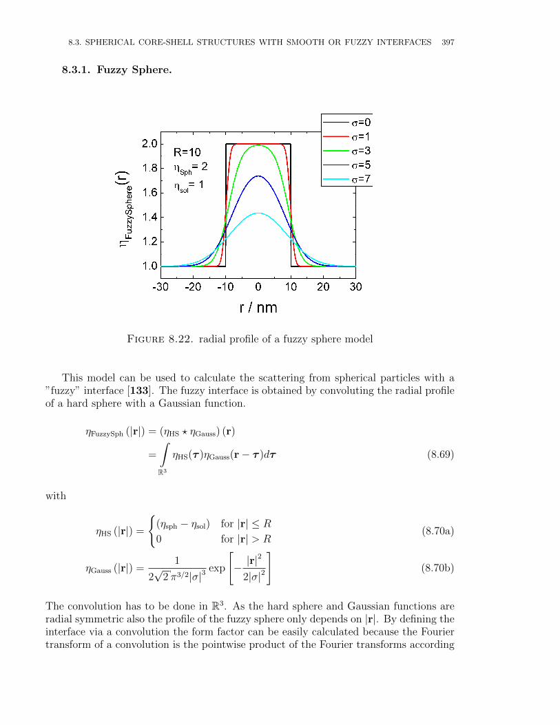
8.3. SPHERICAL CORE-SHELL STRUCTURES WITH SMOOTH OR FUZZY INTERFACES 397
8.3.1. Fuzzy Sphere.
Figure 8.22. radial profile of a fuzzy sphere model
This model can be used to calculate the scattering from spherical particles with a”fuzzy” interface [133]. The fuzzy interface is obtained by convoluting the radial profileof a hard sphere with a Gaussian function.
ηFuzzySph (|r|) = (ηHS ? ηGauss) (r)
=
∫R3
ηHS(τ )ηGauss(r− τ )dτ (8.69)
with
ηHS (|r|) =
(ηsph − ηsol) for |r| ≤ R
0 for |r| > R(8.70a)
ηGauss (|r|) =1
2√
2 π3/2|σ|3exp
[− |r|
2
2|σ|2
](8.70b)
The convolution has to be done in R3. As the hard sphere and Gaussian functions areradial symmetric also the profile of the fuzzy sphere only depends on |r|. By defining theinterface via a convolution the form factor can be easily calculated because the Fouriertransform of a convolution is the pointwise product of the Fourier transforms according
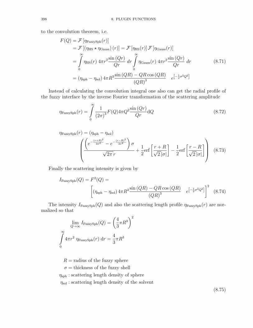
398 8. PLUGIN FUNCTIONS
to the convolution theorem, i.e.
F (Q) = F [ηFuzzySph(r)]
= F [(ηHS ? ηGauss) (r)] = F [ηHS(r)]F [ηGauss(r)]
=
∞∫0
ηHS(r) 4πr2 sin (Qr)
Qrdr
∞∫0
ηGauss(r) 4πr2 sin (Qr)
Qrdr
= (ηsph − ηsol) 4πR3 sin (QR)−QR cos (QR)
(QR)3 e[−12σ2Q2]
(8.71)
Instead of calculating the convolution integral one also can get the radial profile ofthe fuzzy interface by the inverse Fourier transformation of the scattering amplitude
ηFuzzySph(r) =
∞∫0
1
(2π)3F (Q)4πQ2 sin (Qr)
QrdQ (8.72)
ηFuzzySph(r) = (ηsph − ηsol)(e−
(r+R)2
2σ2 − e−(r−R)2
2σ2
)σ
√2π r
+1
2erf
[r +R√
2 |σ|
]− 1
2erf
[r −R√
2 |σ|
] (8.73)
Finally the scattering intensity is given by
IFuzzySph(Q) = F 2(Q) =[(ηsph − ηsol) 4πR3 sin (QR)−QR cos (QR)
(QR)3 e[−12σ2Q2]
]2
(8.74)
The intensity IFuzzySph(Q) and also the scattering length profile ηFuzzySph(r) are nor-malized so that
limQ→∞
IFuzzySph(Q) =
(4
3πR3
)2
∞∫0
4πr2 ηFuzzySph(r) dr =4
3πR3
R = radius of the fuzzy sphere
σ = thickness of the fuzzy shell
ηsph : scattering length density of sphere
ηsol : scattering length density of the solvent
(8.75)
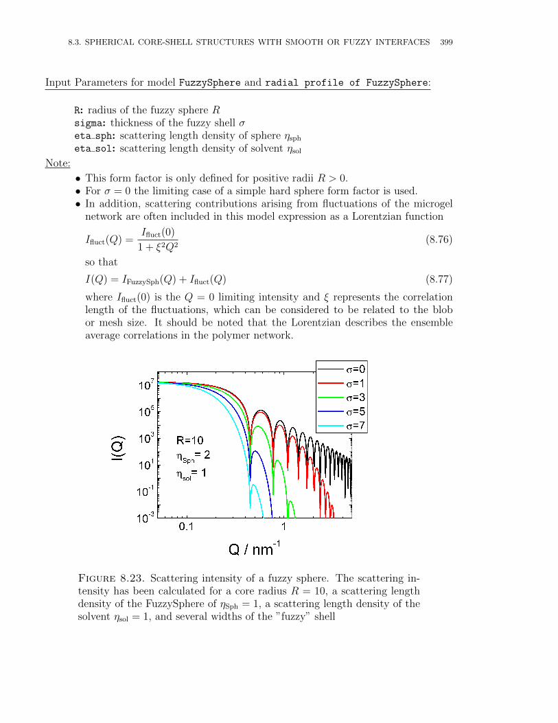
8.3. SPHERICAL CORE-SHELL STRUCTURES WITH SMOOTH OR FUZZY INTERFACES 399
Input Parameters for model FuzzySphere and radial profile of FuzzySphere:
R: radius of the fuzzy sphere Rsigma: thickness of the fuzzy shell σeta sph: scattering length density of sphere ηsph
eta sol: scattering length density of solvent ηsol
Note:
• This form factor is only defined for positive radii R > 0.• For σ = 0 the limiting case of a simple hard sphere form factor is used.• In addition, scattering contributions arising from fluctuations of the microgel
network are often included in this model expression as a Lorentzian function
Ifluct(Q) =Ifluct(0)
1 + ξ2Q2(8.76)
so that
I(Q) = IFuzzySph(Q) + Ifluct(Q) (8.77)
where Ifluct(0) is the Q = 0 limiting intensity and ξ represents the correlationlength of the fluctuations, which can be considered to be related to the blobor mesh size. It should be noted that the Lorentzian describes the ensembleaverage correlations in the polymer network.
Figure 8.23. Scattering intensity of a fuzzy sphere. The scattering in-tensity has been calculated for a core radius R = 10, a scattering lengthdensity of the FuzzySphere of ηSph = 1, a scattering length density of thesolvent ηsol = 1, and several widths of the ”fuzzy” shell

400 8. PLUGIN FUNCTIONS
(a) radial profile of a sphere with a parabolicinterface
(b) radial profile of a spherical shell with par-abolic interfaces
Figure 8.24. .....
8.3.2. CoreShellMicrogel. This model can be used to calculate the scatteringfrom spherical particles with a parabolic ”fuzzy” interface [10, 9, 11]. The radial profileis given by
ρ(r, R, σ) =
1 for r ≤ R− σ1− 1
2((r−R)+σ)2
σ2 for R− σ < r ≤ R12
((R−r)+σ)2
σ2 for R < r ≤ R + σ
0 for r >≤ R + σ
(8.78)
where R = W +σ. For such a radial profile the Fourier-transformation can be calculatedanalytically as
F (Q,R, σ) = F [ρ(r, R, σ)] =
4π
((R
σ2+
1
σ
)cos(q(R + σ))
q4+
(R
σ2− 1
σ
)cos(q(R− σ))
q4
− 3sin(q(R + σ))
q5σ2− 3
sin(q(R− σ))
q5σ2− 6
sin(qR)
q5σ2− 2R
cos(qR)
q4σ2
)(8.79)
The last term in the brackets needed to be corrected compared to the papers mentionedabove due to a typo in the original papers. The radial scattering length density profileof a fuzzy core shell like in Fig. 8.24b can be obtained by
ηcore,sh(r,Wcore, σcore, D, σsh,in,Wsh, σsh,out) = ηsol + (ηshell − ηsol)ρ(r, Rout, σout)
+ (ηshell − ηsol)ρ(r, Rsh,in, σsh,in) + (ηcore − ηsol)ρ(r, Rcore, σcore) (8.80)
8.3. SPHERICAL CORE-SHELL STRUCTURES WITH SMOOTH OR FUZZY INTERFACES 401
with
Rcore = Wcore + σcore (8.81a)
Rsh,in = Rcore +D (8.81b)
Rout = Rsh,in + σsh,in +Wsh + σsh,out (8.81c)
In the same way also the scattering amplitude Fcore,sh(Q, · · · ) and the scattering intensity
Icore,sh(Q, · · · ) = |Fcore,sh(Q, · · · )|2 can be calculated
Fcore,sh(Q,Wcore, σcore, D, σsh,in,Wsh, σsh,out) = (ηshell − ηsol)F (Q,Rout, σout)
+ (ηshell − ηsol)F (Q,Rsh,in, σsh,in) + (ηcore − ηsol)F (Q,Rcore, σcore) (8.82a)
Icore,sh(Q,Wcore, σcore, D, σsh,in,Wsh, σsh,out) = |Fcore,sh(Q, · · · )|2 (8.82b)
Input parameters for ”CoreShellMicrogel” and ”radial profile of
CoreShellMicrogel”:
W core: radius of center parts of core Wcore with homogeneous scattering lengthdensity
sigma core: interface half width of the core σcore
W shell: width of center parts of shell Wsh with homogeneous scattering lengthdensity
sigma sh,in: half width of the inner interface of shell σsh,in
D: distance D between interface of core and in interface of shellsigma out: half width of the outer surface profile σout
eta core: scattering length density of homogeneous core part ηcore
eta shell: scattering length density of homogeneous shell part ηshell
eta sol: scattering length density of solvent ηsol
Note
• If one like to simulate a simple step profile one should set D = 0 and σcore =σsh,in. The last equality in case of fitting this parameter can be simply obtainedby a global parameter under fitting multiple data sets.• Instead of using the radii in eq. 8.81 as input parameters the thickness of the
homogeneous parts of the core and the shell have been used to avoid a problems(negative dimensions) by applying an integration over a size distribution startingfrom 0 on the radii.

402 8. PLUGIN FUNCTIONS
(a) Some radial profiles of spheres with a par-abolic interfaces which have been used to cal-culate the scattering curve in Fig. (b).
(b) Scattering curves of the radial profiles
shown in Fig. (a).
Figure 8.25. The profiles and scattering curves hve been calculatedwith the plugin functions ”CoreShellMicrogel” and ”Radial Profile
of CoreShellMicrogel”.
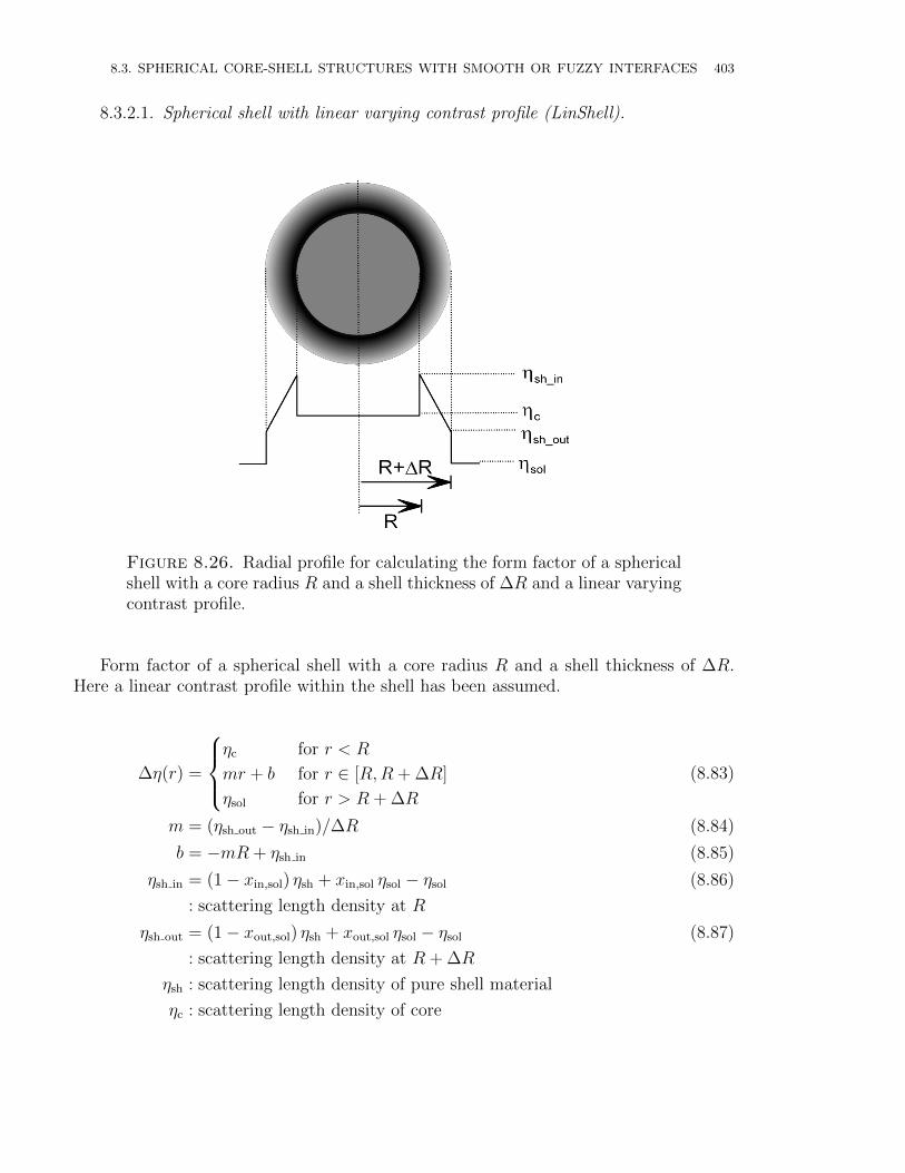
8.3. SPHERICAL CORE-SHELL STRUCTURES WITH SMOOTH OR FUZZY INTERFACES 403
8.3.2.1. Spherical shell with linear varying contrast profile (LinShell).
Figure 8.26. Radial profile for calculating the form factor of a sphericalshell with a core radius R and a shell thickness of ∆R and a linear varyingcontrast profile.
Form factor of a spherical shell with a core radius R and a shell thickness of ∆R.Here a linear contrast profile within the shell has been assumed.
∆η(r) =
ηc for r < R
mr + b for r ∈ [R,R + ∆R]
ηsol for r > R + ∆R
(8.83)
m = (ηsh out − ηsh in)/∆R (8.84)
b = −mR + ηsh in (8.85)
ηsh in = (1− xin,sol) ηsh + xin,sol ηsol − ηsol (8.86)
: scattering length density at R
ηsh out = (1− xout,sol) ηsh + xout,sol ηsol − ηsol (8.87)
: scattering length density at R + ∆R
ηsh : scattering length density of pure shell material
ηc : scattering length density of core
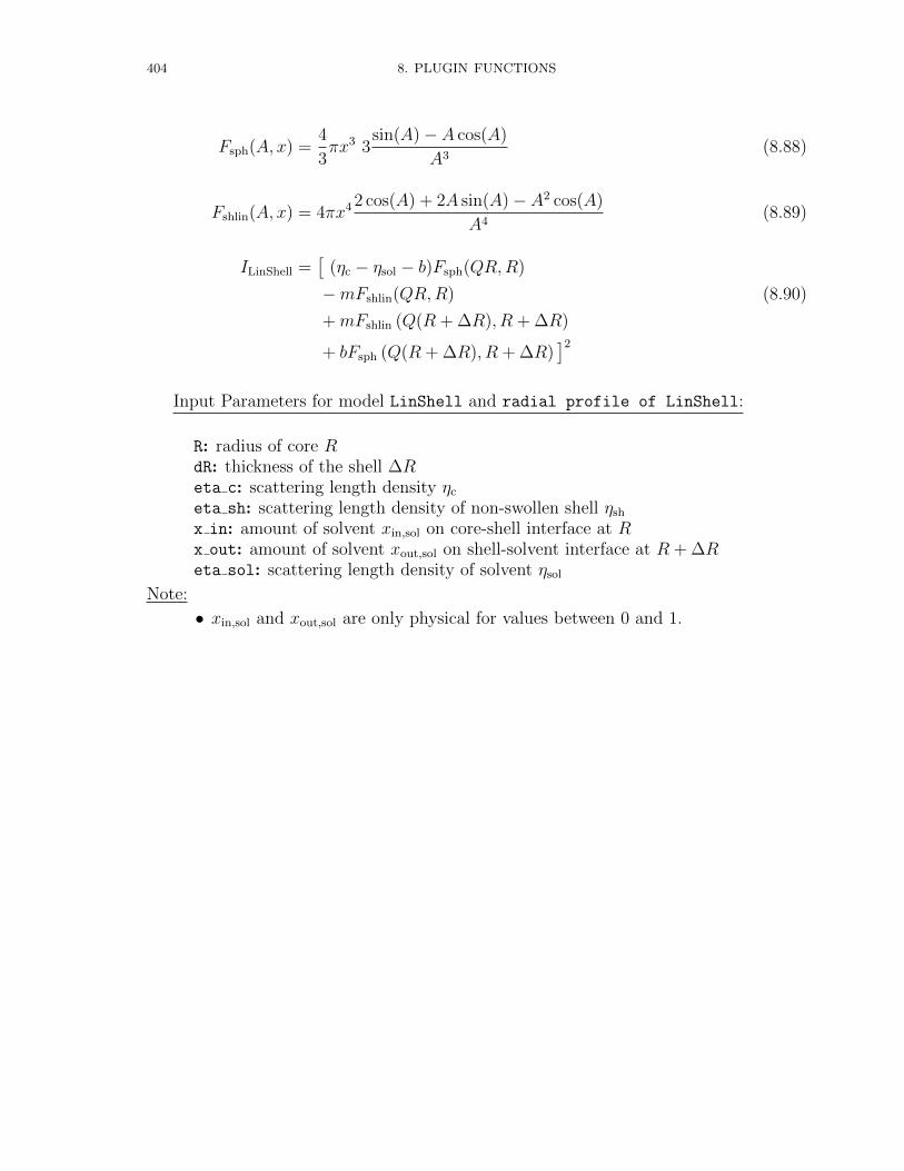
404 8. PLUGIN FUNCTIONS
Fsph(A, x) =4
3πx3 3
sin(A)− A cos(A)
A3(8.88)
Fshlin(A, x) = 4πx4 2 cos(A) + 2A sin(A)− A2 cos(A)
A4(8.89)
ILinShell =[
(ηc − ηsol − b)Fsph(QR,R)
−mFshlin(QR,R) (8.90)
+mFshlin (Q(R + ∆R), R + ∆R)
+ bFsph (Q(R + ∆R), R + ∆R)]2
Input Parameters for model LinShell and radial profile of LinShell:
R: radius of core RdR: thickness of the shell ∆Reta c: scattering length density ηc
eta sh: scattering length density of non-swollen shell ηsh
x in: amount of solvent xin,sol on core-shell interface at Rx out: amount of solvent xout,sol on shell-solvent interface at R + ∆Reta sol: scattering length density of solvent ηsol
Note:
• xin,sol and xout,sol are only physical for values between 0 and 1.

8.3. SPHERICAL CORE-SHELL STRUCTURES WITH SMOOTH OR FUZZY INTERFACES 405
(a) Some radial profiles of spheres with a linearinterface profiles due to penetration of solventinto the shell which have been used to calcu-late the scattering curve in Fig. (b).
(b) Scattering curves of the radial profiles
shown in Fig. (a).
Figure 8.27. Scattering intensity of a spherical shell with an linear shellprofile. The scattering intensity has been calculated with a lognormal sizedistribution for the core radius Rc.
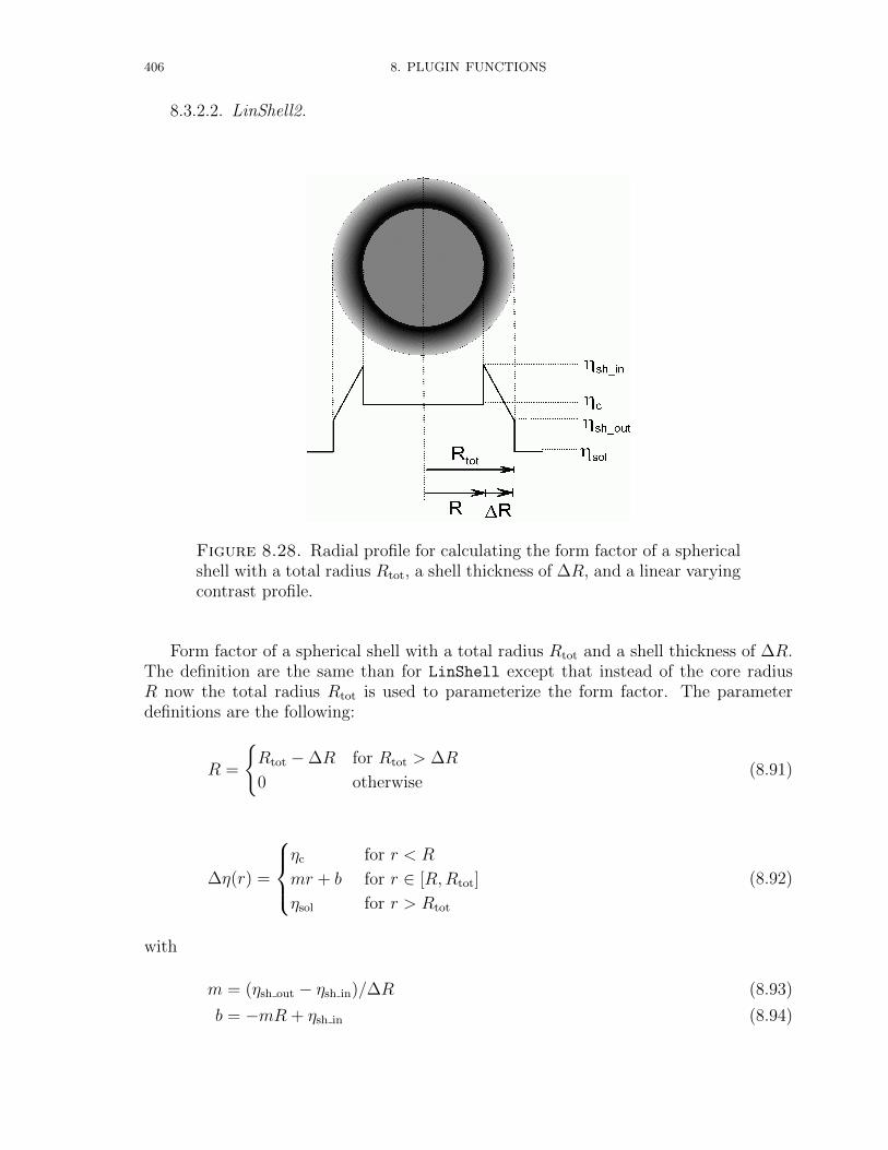
406 8. PLUGIN FUNCTIONS
8.3.2.2. LinShell2.
Figure 8.28. Radial profile for calculating the form factor of a sphericalshell with a total radius Rtot, a shell thickness of ∆R, and a linear varyingcontrast profile.
Form factor of a spherical shell with a total radius Rtot and a shell thickness of ∆R.The definition are the same than for LinShell except that instead of the core radiusR now the total radius Rtot is used to parameterize the form factor. The parameterdefinitions are the following:
R =
Rtot −∆R for Rtot > ∆R
0 otherwise(8.91)
∆η(r) =
ηc for r < R
mr + b for r ∈ [R,Rtot]
ηsol for r > Rtot
(8.92)
with
m = (ηsh out − ηsh in)/∆R (8.93)
b = −mR + ηsh in (8.94)
8.3. SPHERICAL CORE-SHELL STRUCTURES WITH SMOOTH OR FUZZY INTERFACES 407
and
ηsh in = (1− xin,sol) ηsh + xin,sol ηsol (8.95)
: scattering length density at R
ηsh out = (1− xout,sol) ηsh + xout,sol ηsol (8.96)
: scattering length density at Rtot = R + ∆R
ηsh : scattering length density of pure shell material
ηc : scattering length density of core
xin,sol : amount of solvent at R
xout,sol : amount of solvent at Rtot = R + ∆R
Fsph(A, x) =4
3πx3 3
sin(A)− A cos(A)
A3(8.97)
Fshlin(A, x) = 4πx4 2 cos(A) + 2A sin(A)− A2 cos(A)
A4(8.98)
ILinShell2 =[
(ηc − ηsol − b)Fsph(QR,R)
−mFshlin(QR,R) (8.99)
+mFshlin (QRtot, Rtot)
+ bFsph (QRtot, Rtot)]2
Input Parameters for model LinShell2 and radial profile of LinShell2:
Rtot: total overall radius Rtot
dR: thickness of the shell ∆Reta c: scattering length density ηc
eta sh: scattering length density of non-swollen shell ηsh
x in: amount of solvent xin,sol on core-shell interface at R (xin,sol ∈ [0; 1])x out: amount of solvent xout,sol on shell-solvent interface at R + ∆R (xout,sol ∈
[0; 1]).eta s: scattering length density of solvent ηsol
Note:
• xin,sol and xout,sol are only physical for values between 0 and 1.
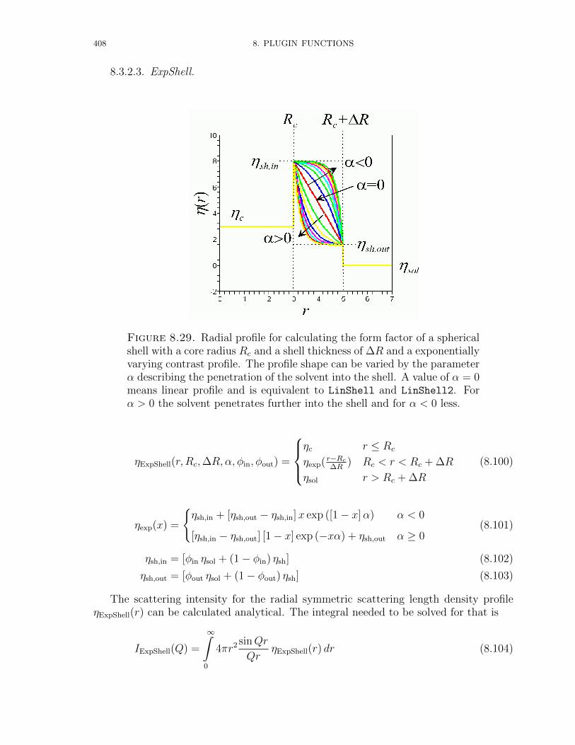
408 8. PLUGIN FUNCTIONS
8.3.2.3. ExpShell.
Figure 8.29. Radial profile for calculating the form factor of a sphericalshell with a core radius Rc and a shell thickness of ∆R and a exponentiallyvarying contrast profile. The profile shape can be varied by the parameterα describing the penetration of the solvent into the shell. A value of α = 0means linear profile and is equivalent to LinShell and LinShell2. Forα > 0 the solvent penetrates further into the shell and for α < 0 less.
ηExpShell(r, Rc,∆R,α, φin, φout) =
ηc r ≤ Rc
ηexp( r−Rc∆R
) Rc < r < Rc + ∆R
ηsol r > Rc + ∆R
(8.100)
ηexp(x) =
ηsh,in + [ηsh,out − ηsh,in]x exp ([1− x]α) α < 0
[ηsh,in − ηsh,out] [1− x] exp (−xα) + ηsh,out α ≥ 0(8.101)
ηsh,in = [φin ηsol + (1− φin) ηsh] (8.102)
ηsh,out = [φout ηsol + (1− φout) ηsh] (8.103)
The scattering intensity for the radial symmetric scattering length density profileηExpShell(r) can be calculated analytical. The integral needed to be solved for that is
IExpShell(Q) =
∞∫0
4πr2 sinQr
QrηExpShell(r) dr (8.104)
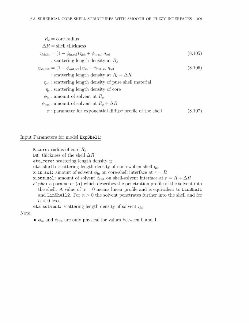
8.3. SPHERICAL CORE-SHELL STRUCTURES WITH SMOOTH OR FUZZY INTERFACES 409
Rc = core radius
∆R = shell thickness
ηsh,in = (1− φin,sol) ηsh + φin,sol ηsol (8.105)
: scattering length density at Rc
ηsh,out = (1− φout,sol) ηsh + φout,sol ηsol (8.106)
: scattering length density at Rc + ∆R
ηsh : scattering length density of pure shell material
ηc : scattering length density of core
φin : amount of solvent at Rc
φout : amount of solvent at Rc + ∆R
α : parameter for exponential diffuse profile of the shell (8.107)
Input Parameters for model ExpShell:
R core: radius of core Rc
DR: thickness of the shell ∆Reta core: scattering length density ηc
eta shell: scattering length density of non-swollen shell ηsh
x in sol: amount of solvent φin on core-shell interface at r = Rx out sol: amount of solvent φout on shell-solvent interface at r = R + ∆Ralpha: a parameter (α) which describes the penetration profile of the solvent into
the shell. A value of α = 0 means linear profile and is equivalent to LinShell
and LinShell2. For α > 0 the solvent penetrates further into the shell and forα < 0 less.
eta solvent: scattering length density of solvent ηsol
Note:
• φin and φout are only physical for values between 0 and 1.
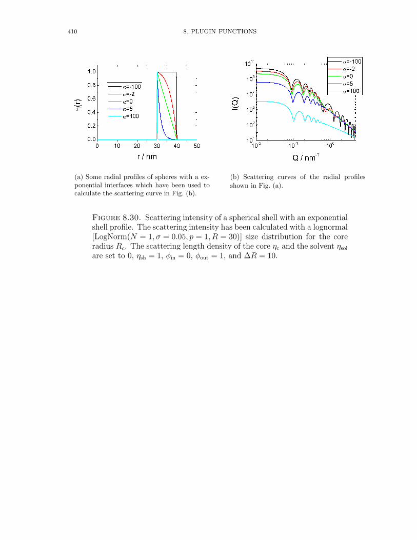
410 8. PLUGIN FUNCTIONS
(a) Some radial profiles of spheres with a ex-ponential interfaces which have been used tocalculate the scattering curve in Fig. (b).
(b) Scattering curves of the radial profiles
shown in Fig. (a).
Figure 8.30. Scattering intensity of a spherical shell with an exponentialshell profile. The scattering intensity has been calculated with a lognormal[LogNorm(N = 1, σ = 0.05, p = 1, R = 30)] size distribution for the coreradius Rc. The scattering length density of the core ηc and the solvent ηsol
are set to 0, ηsh = 1, φin = 0, φout = 1, and ∆R = 10.
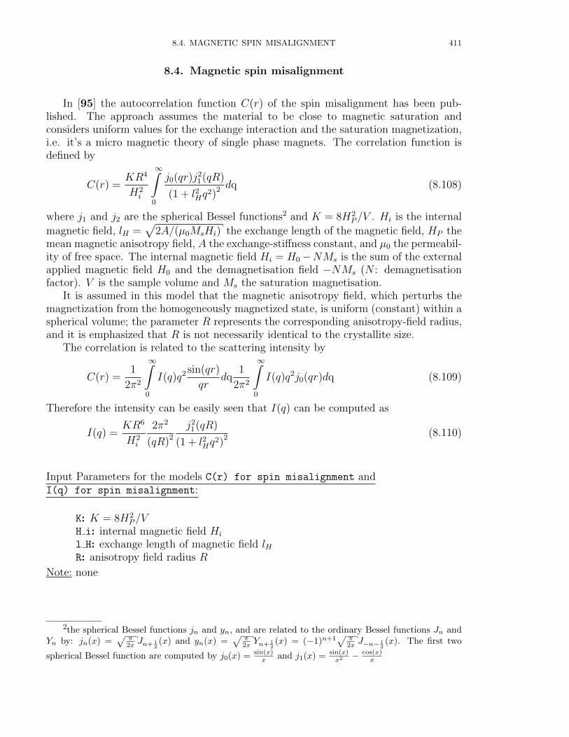
8.4. MAGNETIC SPIN MISALIGNMENT 411
8.4. Magnetic spin misalignment
In [95] the autocorrelation function C(r) of the spin misalignment has been pub-lished. The approach assumes the material to be close to magnetic saturation andconsiders uniform values for the exchange interaction and the saturation magnetization,i.e. it’s a micro magnetic theory of single phase magnets. The correlation function isdefined by
C(r) =KR4
H2i
∞∫0
j0(qr)j21(qR)
(1 + l2Hq2)
2 dq (8.108)
where j1 and j2 are the spherical Bessel functions2 and K = 8H2P/V . Hi is the internal
magnetic field, lH =√
2A/(µ0MsHi) the exchange length of the magnetic field, HP themean magnetic anisotropy field, A the exchange-stiffness constant, and µ0 the permeabil-ity of free space. The internal magnetic field Hi = H0−NMs is the sum of the externalapplied magnetic field H0 and the demagnetisation field −NMs (N : demagnetisationfactor). V is the sample volume and Ms the saturation magnetisation.
It is assumed in this model that the magnetic anisotropy field, which perturbs themagnetization from the homogeneously magnetized state, is uniform (constant) within aspherical volume; the parameter R represents the corresponding anisotropy-field radius,and it is emphasized that R is not necessarily identical to the crystallite size.
The correlation is related to the scattering intensity by
C(r) =1
2π2
∞∫0
I(q)q2 sin(qr)
qrdq
1
2π2
∞∫0
I(q)q2j0(qr)dq (8.109)
Therefore the intensity can be easily seen that I(q) can be computed as
I(q) =KR6
H2i
2π2
(qR)2
j21(qR)
(1 + l2Hq2)
2 (8.110)
Input Parameters for the models C(r) for spin misalignment andI(q) for spin misalignment:
K: K = 8H2P/V
H i: internal magnetic field Hi
l H: exchange length of magnetic field lHR: anisotropy field radius R
Note: none
2the spherical Bessel functions jn and yn, and are related to the ordinary Bessel functions Jn andYn by: jn(x) =
√π2x Jn+ 1
2(x) and yn(x) =
√π2x Yn+ 1
2(x) = (−1)n+1
√π2x J−n− 1
2(x). The first two
spherical Bessel function are computed by j0(x) = sin(x)x and j1(x) = sin(x)
x2 − cos(x)x
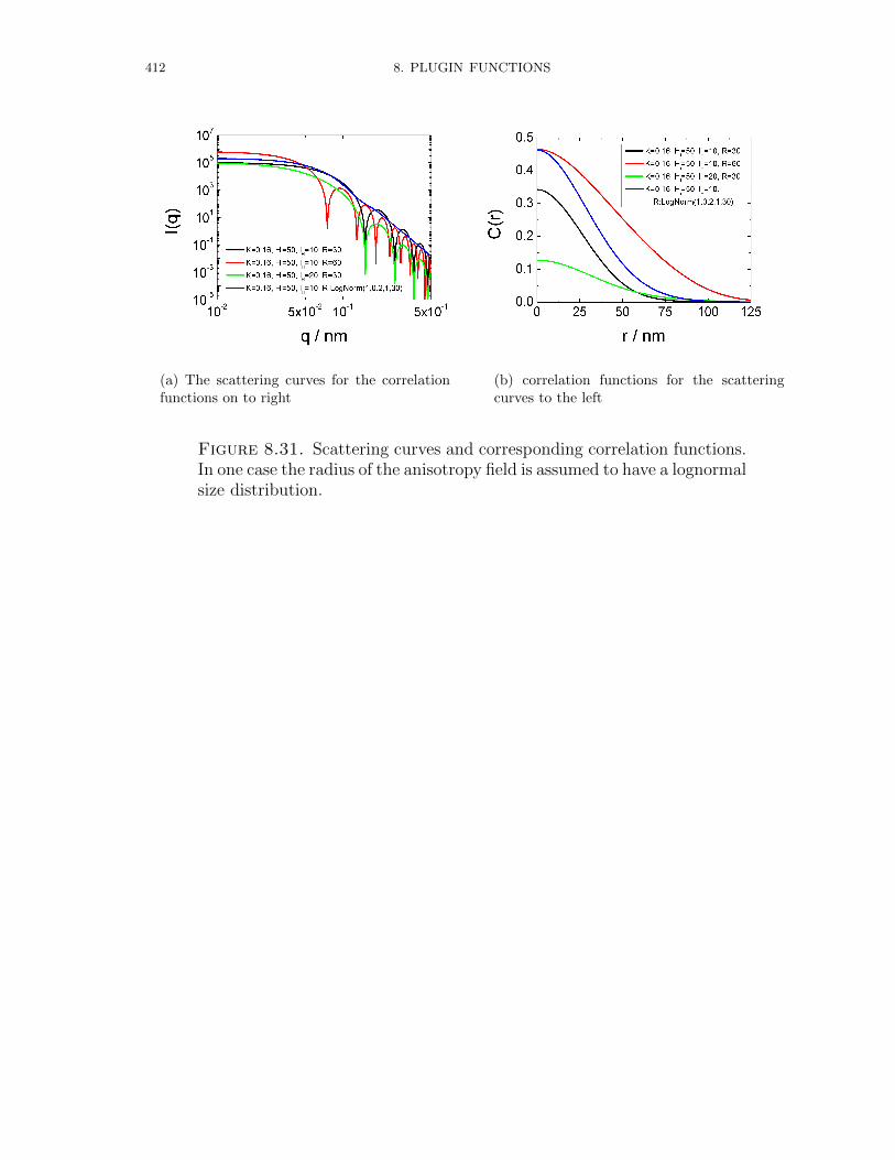
412 8. PLUGIN FUNCTIONS
(a) The scattering curves for the correlationfunctions on to right
(b) correlation functions for the scatteringcurves to the left
Figure 8.31. Scattering curves and corresponding correlation functions.In one case the radius of the anisotropy field is assumed to have a lognormalsize distribution.

8.5. FERROFLUIDS 413
8.5. Ferrofluids
”Ferrofluids” and ”Magnetic Liquids” are two common expressions for suspensionsin which nanometer sized particles are dispersed in a carrier liquid. Figure 8.32 givesa schematic illustration. The particle material can be ferri- or ferromagnetic, and isoften coated with a stabilizing dispersing agent (surfactant). The particle size is smallerthan the size of magnetic domains of the corresponding bulk material. This means thatevery particle is single-domain ferri- or ferromagnetic. Additionally we assume in thismodel, that the metallic core has a shell structure to be able to model a thin oxidationlayer with a reduced magnetisation on the surface.The surfactant molecules consist ofa head and a polar tail. The head can coalesce with the magnetic particle, and thetail protrudes into the carrier liquid and can dissolve in it. This polar tails protrudinginto the liquid lead to repulsion between the colloids. Different substances like organicacids or polymers usually serve as surfactants. The carrier liquid is selected to meetthe requirements for a particular applications: It can be hydrocarbon, ester, water orothers. As a result of the small size of the particles they are very mobile due to Brownianmotion. In zero field the magnetic moment is random oriented. Applying a magneticfield the orientation distribution of the magnetic moments of the ferrofluid particlesfollow a Langevin statistic.
Figure 8.32. Sketch of a ferrofluid particle stabilised with surfactantmolecules on its surface. The magnetic core can have a shell with lowermagnetisation. The direction of the shell magnetisation is assumed to beparallel or antiparallel to the core magnetisation, depending on the signsof the magnetic scattering length densities.
In the present implementation of scattering function of superparamagnetic particlesgeometrical parameters are calculated like magnetic scattering length densities are cal-culated from the magnetization of the shell and the core, whereas the nuclear scattering
414 8. PLUGIN FUNCTIONS
length densities are an explicit input parameter. In such a case one has to be carefulusing the right units.
The relevant parameters to describe the ferrofluid particle in this model are:
• Radius of the Rcore in reciprocal units of scattering vector q.• Thickness of the metallic shell tshell in reciprocal units of scattering vector q.• Specific aggregation number of stabilizing surfactant molecules per surface area
in units of cm−2.• Molecular volume Vbrush of a single surfactant molecule in units of nm3. The
scattering length density calculator of SASfit might be useful to supply thisvalue.• Nuclear scattering length density ηcore of the solid ferromagnetic core.• Nuclear scattering length density ηsh of an optional demagnetised shell of the
solid ferromagnetic core.• Nuclear scattering length density of the solvent ηsolv.• Magnetisation of the metallic coreMcore. The magnetic scattering length density
is calculated via eq. 8.111.• Magnetisation of the metallic shell Msh. Also here the magnetic scattering
length density of the shell is calculated via eq. 8.111.• Temperature T in Kelvin.• External applied magnetic field B in Tesla or milliTesla depending of the units
of q.• Lagrange parameter α for describing superparamagnetic properties is calculated
by ratio of the potential energy of the total magnetic moment of the superpara-magnetic particle in the applied magnetic field to the thermal energy via eq.8.114• As aligned magnetic structures scatter anisotropically the angle ψ between scat-
tering vector and the applied magnetic field needs to be supplied.• using polarised neutrons the incident polarisation p needs to be known. p can
have values p ∈ [−1, 1].• in case of full polarisation analysis also the transmission of the analyser needs
to be known
The magnetic scattering length density ηmag in units of cm−2 is calculated from themagnetisation M given in units of A/m by
ηmag = DMµ0M × 10−4 (8.111)
DM = 2.31611
Vs(8.112)
µ0 = 4π × 10−7Hm−1 = 4π × 10−7 Vs
Am(8.113)
To get the magnetic scattering length density in cm−2 a multiplication factor of 10−4
has to be applied. By choosing the unit cm−2 for the magnetic scattering length densitywe have to use the corresponding units for the nuclear scattering length densities.
The other unit which has to be chosen with care is the molecular volume Vbrush of asingle surfactant molecule. From the specific aggregation and the molecular volume theexcess scattering of the surfactant shell is calculated. In case that the q-values are given

8.5. FERROFLUIDS 415
in units of nm−1 the molecular volume has to be in units of nm3 and in case of A−1 forthe q-values one also need to use A3 units for the molecular volume.
The next parameter, where we need to use proper units is the Langevin parameterα, describing the ratio between potential energy of the magnetic moment of the particleto the thermal energy:
α = µFFB/(kBT ) (8.114)
µFF =4
3π[R3
coreMcore +
(Rcore + tshell)3 −R3
core
Mshell
]× 10−27m3
nm3(8.115)
kB = 1.3806488× 10⁻²³m2kg s−2K−1 (8.116)
The magnetic moment of a particle µFF as given in eq. 8.115 is calculated from the mag-netisation of the core and the shell and their corresponding dimensions. The magnetisa-tion has units of A/m whereas the radius and shell thickness have reciprocal dimensionsof q. A magnetic moment is measured in amperesquare meters (Am2) or in joules pertesla (JT−1) which is equivalent: 1Am2 = 1JT−1. In case that q values are given in A−1
the applied magnetic field should be given in units of mT instead of T.The implemented form factor for ferrofluids is done for neutrons with or without
incident polarisation as well as with polarisation analysis. In case of full polarisationanalysis the measured intensity Im(Q) would depend on the incident polarisation, effi-ciency of the spin-flipper and in case of an opaque spin filter from its transmission valuesfor the two spin states according to eq. 3.304. However here we just have implementedthe intensities for a given incident polarisation without polarisation analysis (SANSPOL)and the intensities for POLARIS data are assumed to be corrected so that the resultingintensities correspond to perfect incident polarisation and perfect polarisation analysis.For calculating the scattering cross-section for the 4 scattering processes involved thedifferential cross-sections in the decoupling approach are given by
dσ±±±∓
dΩ(Q) = N
⟨∣∣∣F±±±∓
(Q)∣∣∣2⟩+
∣∣∣⟨F±±±∓
(Q)⟩∣∣∣2(S(Q)− 1)
(8.117)
The averages 〈〉 needs to be performed over the orientation distribution of the super-paramagnetic moments of the ferrofluids and later on also about their size distribution.The averaging over the orientation distribution of the magnetic moments can be doneanalytically in terms of order parameters according to [150, 146, 73].
The spin dependent scattering amplitudes F±±±∓
(Q) can be calculated from the nuclear
and magnetic amplitudes
F±±(Q) = FN(Q)∓ FM⊥x(Q) (8.118)
F±∓(Q) = − (FM⊥y(Q)± ıFM⊥z(Q)) (8.119)
The nuclear scattering amplitude is proportional to the nuclear excess scattering βN =FN(Q = 0) and the nuclear form factor fN(Q)
FN(Q) = βNfN(Q) (8.120)
The magnetic scattering amplitude FM⊥(Q) can be described as a vector, with
FM⊥(Q) = µ⊥DMµFFfM(Q) = µ⊥FM(Q) (8.121)
416 8. PLUGIN FUNCTIONS
where fM(Q) is the magnetic form factor, µFF the magnetic moment of the particle,DM = γe
2π~ , and µ⊥ the Halpern-Johnson vector defined as
µ⊥ =Q
Q×(µFF
µFF
)(8.122)
It is assumed here that the neutron spin polarization is parallel or antiparallel to theaxes ex which is the direction perpendicular to the incoming neutron beam.
In the following we derive the average over the squared scattering amplitude andthe averaged scattering amplitude for superparamagnetic particles. The description ofthe nuclear scattering amplitude is based on the form factor described in [112, 113] forblock copolymer micelles from Pedersen et al.
The different versions of form factor implemented in the plugin differ on one side onthe model for describing the scattering of the molecules on the surface and on the otherside how the data are pre-treated. At the moment three different model for the polymerchains on the surface are implemented, namely that the chains are noninteracting andfollow random walk behaviour (Chain,RW), secondly they are interacting due to the highgrafting density and a model for self avoiding walk (Chain,SAW) is applied, thirdly aparabolic scattering length density profile for the outer shell is used (Chain,parabolic).For each models a version for a sector cut in the direction ψ (psi), a radial averagedintensity (rad. avg.), the anisotropic scattering contribution, which follows a sin2-law(magnetic), the angle dependent difference signal between two spin states (cross-term),as well as the radial averaged cross term (cross-term (rad. avg.)) has bee imple-mented. Also the for individual angle dependent cross-sections with full polarisationanalysis are available. Finally we end up with the following possible combinations:
FF+(Chain,RW)
FF+(Chain,SAW)
FF+(Chain,parabolic)
−
psi
(rad. avg.)
magnetic
cross-term
cross-term (rad. avg.)
(++)
(--)
(+-)
(-+)
(8.123)
8.5.1. Langevin statistics for averages of the form factor and averages ofthe squared form factor.
It is assumed here that the neutron spin polarization is parallel or antiparallel tothe axes ex which is the direction perpendicular to the incoming neutron beam. Ifonly the Halpern-Johnson vector µ⊥ depends on the orientation distribution f(θ) of themagnetic moments µ of the particles but not the form factor fM(Q), which is valid forspherical symmetric particles or anisotropic shaped particles where the particle shapeis not correlated to the direction of the magnetic moment, the averages in 8.117 can be
8.5. FERROFLUIDS 417
written in terms of the order parameters S1 and S2
〈F±±(Q)〉 = FN(Q) + FM(Q)S1 sin2 ψ (8.124a)
〈F±∓(Q)〉 = FM(Q)S1 sinψ cosψ (8.124b)
⟨|F±±(Q)|2
⟩= |FN(Q)|2 + |FM(Q)|2
[S2 sin4 ψ +
1− S2
3sin2 ψ
]∓ [FM(Q)F ∗N(Q) + F ∗M(Q)FN(Q)]S1 sin2 ψ
(8.124c)
⟨|F±∓(Q)|2
⟩= |FM(Q)|2
[2
1− S2
3− S2 sin4 ψ +
4S2 − 1
3sin2 ψ
](8.124d)
The above equations for the spin dependent scattering intensities of magnetic parti-cles with an orientation distribution f (θ, φ) of its magnetic moment can be calculatedin terms of order parameters Sl if one assumes that the particle are spherical symmetricor the orientation of the magnetic moment of a particle is not correlated to the particleorientation. Furthermore one has to assume that an external magnetic field is appliedperpendicular to the incident neutron beam and that all orientations φ for a given angleθ, which is defined as the angle between the magnetisation vector of the particle and thedirection of the external field B have the same probability, i.e. the orientation distribu-tion only depends on θ so that f (θ, φ) = f (θ). The orientation probability distributionfunction can be expanded in terms of a complete set of orthogonal functions. Expandingit in terms of Legendre polynomials Pl(cos θ) gives
f(θ) =∑l
clPl(cos θ) =∑l
2l + 1
2SlPl(cos θ) (8.125)
The expansion coefficients can be calculated by
cl =2l + 1
2
π∫0
f(θ)Pl(cos θ) sin θ dθ
or
Sl =
π∫0
f(θ)Pl(cos θ) sin θ dθ
(8.126)
The first three Legendre polynomials are defined by
P0(cos θ) = 1 (8.127a)
P1(cos θ) = cos θ (8.127b)
P2(cos θ) =1
2
(3 cos2 θ − 1
)(8.127c)
For superparamagnetic particle the orientation probability distribution is given by
f(θ) =α
4π sinhαexp(α cos θ) (8.128)
418 8. PLUGIN FUNCTIONS
with α = BMpVp/(kBT ) being the Langevin parameter. For this orientation probabilitydistribution the first order parameters can be calculates as
S0 = 1 (8.129a)
S1 = L(α) = cothα− 1
α(8.129b)
S2 = 1− 3L(α)
α(8.129c)
The spin-flip and spin-nonflip cross-sectiondσ±±±∓
dΩ(Q) can be obtained by combin-
ing 8.117 and 8.124. The cross-sections without polarization analysis I±(Q) and forunpolarized neutrons Iunp(Q) are given by
I±(Q) = I±±(Q) + I±∓(Q)
=[|FN(Q)|2 + |FM(Q)|2S2
1 sin2 ψ
∓ [FM(Q)F ∗N(Q) + F ∗M(Q)FN(Q)]S1 sin2 ψ]S(Q)
|FM(Q)|2(
2
3(1− S2) +
(S2 − S2
1
)sin2 ψ
) (8.130a)
Iunp(Q) =1
2(I+(Q) + I−(Q))
=(|FN(Q)|2 + |FM(Q)|2S2
1 sin2 ψ)S(Q)
+ |FM(Q)|2(
2
3(1− S2) +
(S2 − S2
1
)sin2 ψ
) (8.130b)
In the case of a Boltzmann orientation distribution f(θ) = exp(BµkBT
)=
exp(Bµ cos θkBT
)the order parameter Sl already have been given in eq. 8.129 and the spin
dependent intensities can be written as
I±±(Q)
N=∣∣FM(Q)L(α) sin2 ψ ± FN(Q)
∣∣2S(Q) (8.131a)
+ |FM(Q)|2(L(α)
αsin2 ψ −
(L2(α)− 1 + 3
L(α)
α
)sin4 ψ
)
I∓±(Q)
N=(sin2 ψ − sin4 ψ
)L2(α)|FM(Q)|2S(Q) (8.131b)
+ |FM(Q)|2((
sin4 ψ − sin2 ψ)(
L2(α)− 1 + 3L(α)
α
)+ (2− sin2 ψ)
L(α)
α
)ψ is the angle between Q and the horizontal axis in the plane of the detector. L(α) =coth(α)− 1
αis the Langevin function. In the case of a static field the superparamagnetic
8.5. FERROFLUIDS 419
particle are thermodynamic equilibrium and α is given by
α =BMPVPkBT
, (8.132)
with MP being the particle magnetization, VP the particle volume, T the temperaturein Kelvin and kB the Boltzmann constant.
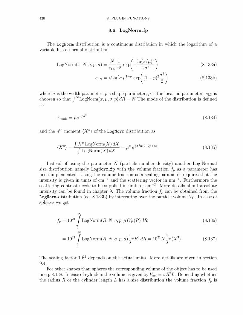
420 8. PLUGIN FUNCTIONS
8.6. LogNorm fp
The LogNorm distribution is a continuous distribuion in which the logarithm of avariable has a normal distribution.
LogNorm(x,N, σ, p, µ) =N
cLN
1
xpexp
(− ln(x/µ)2
2σ2
)(8.133a)
cLN =√
2π σ µ1−p exp
((1− p)2σ
2
2
)(8.133b)
where σ is the width parameter, p a shape parameter, µ is the location parameter. cLN ischoosen so that
∫∞0
LogNorm(x, µ, σ, p) dR = N The mode of the distribution is definedas
xmode = µe−pσ2
(8.134)
and the nth moment 〈Xn〉 of the LogNorm distribution as
〈Xn〉 =
∫Xn LogNorm(X) dX∫
LogNorm(X) dX= µn e
12σ2n(2−2p+n). (8.135)
Instead of using the parameter N (particle number density) another Log-Normalsize distribution namely LogNorm fp with the volume fraction fp as a parameter hasbeen implemented. Using the volume fraction as a scaling parameter requires that theintensity is given in units of cm−1 and the scattering vector in nm−1. Furthermore thescattering contrast needs to be supplied in units of cm−2. More details about absoluteintensity can be found in chapter 9. The volume fraction fp can be obtained from theLogNorm-distribution (eq. 8.133b) by integrating over the particle volume VP . In case ofspheres we get
fp = 1021
∞∫0
LogNorm(R,N, σ, p, µ)VP (R) dR (8.136)
= 1021
∞∫0
LogNorm(R,N, σ, p, µ)4
3πR3 dR = 1021N
4
3π〈X3〉. (8.137)
The scaling factor 1021 depends on the actual units. More details are given in section9.4.
For other shapes than spheres the corresponding volume of the object has to be usedin eq. 8.138. In case of cylinders the volume is given by Vcyl = πR2L. Depending whetherthe radius R or the cylinder length L has a size distribution the volume fraction fp is
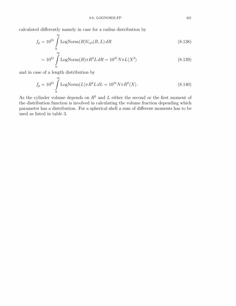
8.6. LOGNORM FP 421
calculated differently namely in case for a radius distribution by
fp = 1021
∞∫0
LogNorm(R)Vcyl(R,L) dR (8.138)
= 1021
∞∫0
LogNorm(R)πR2LdR = 1021NπL〈X2〉 (8.139)
and in case of a length distribution by
fp = 1021
∞∫0
LogNorm(L)πR2LdL = 1021NπR2〈X〉. (8.140)
As the cylinder volume depends on R2 and L either the second or the first moment ofthe distribution function is involved in calculating the volume fraction depending whichparameter has a distribution. For a spherical shell a sum of different moments has to beused as listed in table 3.
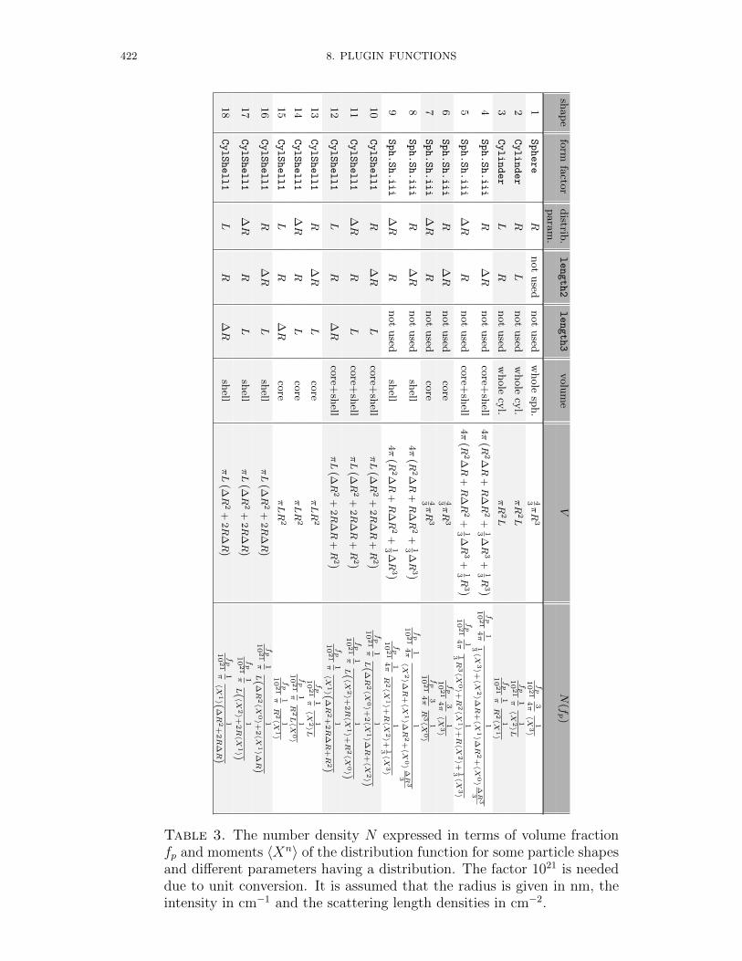
422 8. PLUGIN FUNCTIONS
shap
efo
rmfa
ctor
distrib
.length2
length3
volu
me
VN
(fp )
para
m.
1Sphere
Rnot
used
not
used
whole
sph.
43πR
3fp
1021
34π
1〈X
3〉
2Cylinder
RL
not
used
whole
cyl.
πR
2L
fp
1021
1π1
〈X
2〉L
3Cylinder
LR
not
used
whole
cyl.
πR
2L
fp
1021
1π1
R2〈X
1〉
4Sph.Sh.iii
R∆R
not
used
core+
shell
4π (R
2∆R
+R
∆R
2+
13∆R
3+
13R
3 )fp
1021
14π
113〈X
3〉+〈X
2〉∆R
+〈X
1〉∆R
2+〈X
0〉∆
R3
3
5Sph.Sh.iii
∆R
Rnot
used
core+
shell
4π (R
2∆R
+R
∆R
2+
13∆R
3+
13R
3 )fp
1021
14π
113R
3〈X
0〉+R
2〈X
1〉+R〈X
2〉+
13〈X
3〉
6Sph.Sh.iii
R∆R
not
used
core
43πR
3fp
1021
34π
1〈X
3〉
7Sph.Sh.iii
∆R
Rnot
used
core
43πR
3fp
1021
34π
1R
3〈X
0〉
8Sph.Sh.iii
R∆R
not
used
shell
4π (R
2∆R
+R
∆R
2+
13∆R
3 )fp
1021
14π
1
〈X
2〉∆R
+〈X
1〉∆R
2+〈X
0〉∆
R3
3
9Sph.Sh.iii
∆R
Rnot
used
shell
4π (R
2∆R
+R
∆R
2+
13∆R
3 )fp
1021
14π
1
R2〈X
1〉+R〈X
2〉+
13〈X
3〉
10
CylShell1
R∆R
Lco
re+sh
ellπL (∆
R2
+2R
∆R
+R
2 )fp
1021
1π1
L(∆R
2〈X
0〉+
2〈X
1〉∆R
+〈X
2〉)11
CylShell1
∆R
RL
core+
shell
πL (∆
R2
+2R
∆R
+R
2 )fp
1021
1π1
L( 〈X
2〉+
2R〈X
1〉+R
2〈X
0〉)12
CylShell1
LR
∆R
core+
shell
πL (∆
R2
+2R
∆R
+R
2 )fp
1021
1π1
〈X
1〉(∆R
2+
2R
∆R
+R
2)13
CylShell1
R∆R
Lco
reπLR
2fp
1021
1π1
〈X
2〉L
14
CylShell1
∆R
RL
core
πLR
2fp
1021
1π1
R2L〈X
0〉
15
CylShell1
LR
∆R
core
πLR
2fp
1021
1π1
R2〈X
1〉
16
CylShell1
R∆R
Lsh
ellπL (∆
R2
+2R
∆R )
fp
1021
1π1
L(∆R
2〈X
0〉+
2〈X
1〉∆R
)17
CylShell1
∆R
RL
shell
πL (∆
R2
+2R
∆R )
fp
1021
1π1
L( 〈X
2〉+
2R〈X
1〉)18
CylShell1
LR
∆R
shell
πL (∆
R2
+2R
∆R )
fp
1021
1π1
〈X
1〉(∆R
2+
2R
∆R
)
Table 3. The number density N expressed in terms of volume fractionfp and moments 〈Xn〉 of the distribution function for some particle shapesand different parameters having a distribution. The factor 1021 is neededdue to unit conversion. It is assumed that the radius is given in nm, theintensity in cm−1 and the scattering length densities in cm−2.
CHAPTER 9
Absolute intensities, moments and volume fractions
9.1. Fitting absolute intensities
Absolute intensities in the simulation can be obtained by using proper units for thescattering vector Q, the size dimensions of the scatterer, the scattering length densitiesetc. In the following a few example are discussed for absolute calibrated data sets.One question which is asked quite frequently is ”What is the meaning of N in the sizedistribution and what are its units?”. The answer is normally ”That depends on theunits of your data you are fitting and the units of your scattering length densities”. Inthe following a few explanations will be given to clarify this in some more detail.
Let us consider first the scattering intensity of a single sphere. The form factor of asphere is given by eq. 3.1a as
ISphere(Q,R,∆η) =
[4
3πR3∆η 3
sinQR−QR cosQR
(QR)3
]2
(9.1)
The radius R and the scattering vector Q have reciprocal units, i.e. if Q is given in 1/nmthe radius R has a unit of nm. The other variable in the form factor is the scatteringlength density contrast ∆η between sphere and surrounding matrix or solvent. The unitof the scattering length density is length/volume and has therefore a unit 1/cm2 or some
other sites are using units of 1/A2. The difference is only a constant factor of
∆η1
cm= 1016∆η
1
A. (9.2)
The overall unit of the scattering intensity (differential cross-section) of a single sphereis therefore
[ISphere(Q,R,∆η)] = [R]6 [∆η]2 =nm6
cm4= 10−42cm2 (9.3)
for the case that [R] = nm and [∆η] = cm−2. The unit for the scattering cross-section
of a single sphere with [R] = A and [∆η] = A−2
is than
[ISphere(Q,R,∆η)] = [R]6 [∆η]2 =A
6
A4 = A
2= 10−16cm2, (9.4)
respectively. The scattering cross-section of a single scatterer is calculated by SASfit ifone chooses in the tab for distribution functions the probability functions Monodisperse.
Differential cross-section have a unit of an area[dΣ
dΩ(Q)
]= cm2. (9.5)
423
424 9. ABSOLUTE INTENSITIES, MOMENTS AND VOLUME FRACTIONS
Many instruments deliver with their data reduction software a cross-section normalizedby the sample volume so that the unit is in reciprocal length:[
dσ
dΩ(Q)
]=
1
[V ]
[dΣ
dΩ(Q)
]=
1
cm. (9.6)
For fitting a form factor to experimental data one needs next to the size parameteralso a scaling parameter. For the simplest case this is done by choosing as a distributionfunction Delta. Delta simply multiplies a constant value N to the form factor. Themeaning and the unit of N now depends on the unit of the cross-section, wether it isnormalized or not normalized on the sample volume. SASfit calculates in the case of aform factor of Sphere with Delta as a distribution function
ISASfit = N × ISphere(Q,R,∆η). (9.7)
Fitting N to a data set, which is given in units of 1/cm and where [Q] = nm−1, [R] = nmand [∆η] = cm−2 would mean that N has the unit
[N ] =
[dσdΩ
(Q)]
[ISphere(Q,R,∆η)(Q)]=
1cm
10−42cm2= 1042cm−3. (9.8)
One therefore needs to multiply the value N obtained by SASfit with 1042 to get thenumber density of scatterers in units of cm−3.
Let us now consider the simplest case of spheres with a size distribution and nostructure factor, which are fitted to experimental data. All the size distribution have ascaling parameter N . The units of the parameter N in the size distribution is the samethan for Delta. The size distribution n(x) are implemented as distribution functionn(x) = Np(x) with p(x) being a probability function. In case of polydisperse spheresSASfit calculates the integral
ISASfit (Q) =
∞∫0
n(R) ISphere(Q,R,∆η) dR (9.9)
= N
∞∫0
p(R) ISphere(Q,R,∆η) dR (9.10)
The probability function p(x) is normalized to∞∫
0
p(x) dx = 1, (9.11)
so that the parameter N has like for the Delta-distribution the unit [N ] = 1042cm−3 ifthe data set is given in units of 1/cm and [Q] = nm−1, [R] = nm and [∆η] = cm−2.
Most of the form factor are implemented in a way that they return the scatteringcross-section of a single object like the example of a sphere above, but a few are not,like for example the standard form of a gaussian chain Gauss. In this particular casetwo other versions Gauss2 and Gauss3 with different parameterizations of the forwardscattering of a single gaussian chain are available. However, there are some form factors,which have been implemented according to the literature but which are normalized
9.2. CONTRAST - CONCENTRATION - FORWARD SCATTERING - PARTICLE VOLUME - ABSOLUTE SCALE425
differently. This has to be checked before the parameter N in the size distribution isinterpreted in terms of number density of scatterers.
9.2. Contrast - Concentration - Forward Scattering - Particle Volume -Absolute Scale
A frequently asked question is if the scattering intensity is consistent with the con-centration of material in the sample. Especially people working with micellar solution,star polymers, but also proteins, etc. want to cross-check the absolute intensity with theknown concentration. In the dilute case the differential cross-section is simply N timesthe cross-section of an individual scatterer
dσ
dΩ(Q) =
N
Vtot
P (Q) (9.12)
N is number of particles/molecules/proteins in the illuminated volume, Vtot the illumi-nated sample volume, n = N/Vtot the particle number density, and P (Q) the scatteringcross-section of a single particle. P (Q) has the dimension cm2, N/Vtot the dimensioncm−3, and dσ
dΩ(Q) the dimension cm−1. Eq. 9.14 can also be expressed in terms of con-
centration c in units of g/cm2
c = n mmol = n Mru = nMrMu
NA
=N
Vtot
MrMu
NA
(9.13)
so that
dσ
dΩ(Q) = c
NA
MrMu
P (Q) (9.14)
Mr is the relative molar mass of the particle 1 (Molecular weight (M.W.) and formulaweight (F.W.) are older terms) which is a dimensionless quantity (i.e., a pure number,without units). To get units in g/mol the relative molar mass needs to be multiplied bythe molar mass constant Mu. The value of the molar mass constant Mu is defined to be 1g/mol in SI units. The molar mass constant is important in writing dimensionally correctequations. It is common to see phrases such as ”The molar mass of an element is theatomic weight in grams per mole.” However molecular or atomic weight are dimensionlessquantities, and cannot take the units of grams per mole. Formally, the operation isthe multiplication by a constant which has the value 1 g/mol, that is the molar massconstant2. The molecule mass mm in units of g is mm = MrMu/NA.
1 Definition of relative atomic mass and relative molecular mass can be found on the url-addresshttp://physics.nist.gov/Pubs/SP811/sec08.html
Relative atomic mass (formerly atomic weight): ratio of the average mass per atom ofan element to 1/12 of the mass of the atom of the nuclide 12C.
Relative molecular mass (formerly molecular weight): ratio of the average mass permolecule or specified entity of a substance to 1/12 of the mass of an atom of the nuclide12C.
2Definition of unified atomic mass unit: 1u = mu = m(12C)/12 = 1Mu/NA =
1 (g/mol) /(6.02214129× 1023mol−1
)= 1.660538921× 10⁻²⁴g
426 9. ABSOLUTE INTENSITIES, MOMENTS AND VOLUME FRACTIONS
Now we need to look on the forward scattering P (Q=0) of a single parti-cle/protein/polymer chain. For a simple particle like a sphere, the forward scattering isgiven by
P (Q=0) = (ηsol − ηsp)2 V 2sp (9.15)
where (ηsol − ηsp) is the scattering contrast between spherical particle and solvent andVsp the volume of a single sphere. In case of a spherical particle the boundary betweenparticle and solvent is well defined and therefore also the volume of the particle as ithas a sharp interface. The scattering contrast of a spherical particle can also be writtenin terms of the overall scattering length of the sphere bsp, i.e. the sum of the scatteringlength of all atoms forming the sphere, the volume of the sphere and the scatteringlength density of the solvent. The volume of the sphere can be calculated from its massmsp or relative molar mass Mr,sp and its density ρsp.
(ηsol − ηsp) =
(ηsol −
bsp
Vsp
)=
(ηsol −
bspρsp
msp
)=
(ηsol −
bspρspNA
Mr,spMu
)(9.16)
But what about the forward scattering of a gaussian polymer coil? A polymer does nothas a sharp boundary to the solvent. Polymer and solvent can penetrate each other.To determine the polymer volume one would need a detailed model for the polymermolecule and its interaction with solvent molecules. As a first approximation the volumeof a polymer molecule can be obtained by Vpolym =
ρpolym
mpolym. For a polymer coil with a
relative molar mass Mr,polym the forward scattering in a solvent is given by
P (Q=0) =
(Mr,polymMu
ρpolymNA
)2(ηsol −
bpolymρpolymNA
Mr,polymMu
)2
(9.17)
The volume of a polymer molecule
Vpolym =Mr,polymMu
ρpolymNA
is the volume occupied by single polymer chain in the solvent or in other word theamount of solvent volume displaced by one polymer chain. For the forward scatteringit does not matter, if the coil is collapsed or swollen. As long as the scattering lengthdensity of the solvent inside the swollen polymer coil is the same than in the bulk andthe molecular volume of the polymer chain does not change with the solvent qualitythe forward scattering does not depend on the conformation of the polymer. Sometimesthe relative molar mass of a polymer is given in degree of polymerization p and relativemolar mass of the monomer Mr,m. In this case and assuming that the mass densities ofpolymer and monomer are the same the forward scattering is given by
P (Q=0) =
(p Mr,mMu
ρmNA
)2(ηsol −
bmρmNA
Mr,mMu
)2
=
(p Mr,mMu
ρmNA
)2(ηsol −
bmρmNA
Mr,mMu
)2
(9.18)
9.3. MOMENTS OF SCATTERING CURVES AND SIZE DISTRIBUTION 427
Let us now come back to the measured differential cross-section dσdΩ
(Q). For Q = 0 weget
dσ
dΩ(Q=0) =
N
Vtot
P (Q=0) = cNA
Mr,GaussMu
P (Q=0) (9.19)
= cNA
p Mr,mMu
(p Mr,mMu
ρmNA
)2(ηsol −
bmρmNA
Mr,mMu
)2
(9.20)
= cp Mr,mMu
NAρ2m
(ηsol −
bmρmNA
Mr,mMu
)2
(9.21)
The last equation says, that the forward scattering of a solution of dilute non-interactingpolymer molecules consisting of p monomer units depends linearly on the number ofmonomer units p in the polymer. Even though the scattering of a single polymer moleculedepends quadratically on on the number of monomer units. The reason is simply thatthe larger the degree of polymerization the lower the number density of molecules in thesolution as we assume a constant concentration, i.e. c ∝ pn and therefore dσ
dΩ(Q=0) ∝
p2n.
9.3. Moments of scattering curves and size distribution
The relevance of moments both for scattering curves as well as size distributions hasbeen discussed in several publications [26, 128, 27, 147, 98, 50].
Moments 〈xm〉 of any order m of a function f(x) are defined by integrating f(x) witha suitable power of x over its domain [a, b]
〈xm〉 =
b∫a
f(x)xmdx (9.22)
The different moments of the scattering curve together with the forward scatteringI(0) and the Porod constant can be used to calculate easily several structural parameters
428 9. ABSOLUTE INTENSITIES, MOMENTS AND VOLUME FRACTIONS
of the scatterers.
Qinv =
∞∫0
Q2I(Q)dQ (scattering invariant) (9.23a)
S
V=
π
Qinv
limQ→∞
Q4I(Q)
(specific surface) (9.23b)
〈RG〉2 = 3
(− lim
Q→0
d[ln I(Q)]
d(Q2)
)(squared Guinier radius) (9.23c)
li = 〈d〉 =4
π
∫∞0Q2I(Q)dQ
limQ→∞
Q4I(Q)
(average intersection length) (9.23d)
lc = 〈l〉 =π
Qinv
∞∫0
QI(Q)dQ (correlation length) (9.23e)
Ac = 〈A〉 =2π
Qinv
∞∫0
I(Q)dQ (correlation surface) (9.23f)
VP = 〈V 〉 =2π2
Qinv
I(0) (correlation volume, Porod volume) (9.23g)
These structural parameters are calculated by SASfit via the menu [Calc|integral
parameters...].On the other side the structural parameters from above can depend on specific mo-
ments of the size distribution in the case the scattering objects are spheres. The m-thmoment 〈xm〉 of a size distribution n(R) is given by
〈Rm〉 =
∞∫0
n(R)RmdR
∞∫0
n(R)dR
(9.24)
From these moments the following integral structural parameters in case of polydis-perse spheres can be calculated and are listed together with a hypothetical radius ofmonodisperse spheres having the same structural parameter.
intersection length li:
li =〈R3〉〈R2〉
and Rli =3
4li
correlation length lc:
lc =〈R4〉〈R3〉
and Rlc =2
3lc
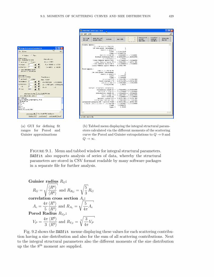
9.3. MOMENTS OF SCATTERING CURVES AND SIZE DISTRIBUTION 429
(a) GUI for defining fitranges for Porod andGuinier approximations
(b) Tabbed menu displaying the integral structural param-eters calculated via the different moments of the scatteringcurve the Porod and Guinier extrapolations to Q→ 0 andQ→∞.
Figure 9.1. Menu and tabbed window for integral structural parameters.SASfit also supports analysis of series of data, whereby the structuralparameters are stored in CSV format readable by many software packagesin a separate file for further analysis.
Guinier radius RG:
RG =
√〈R8〉〈R6〉
and RRG =
√5
3RG
correlation cross section Ac:
Ac =4π
5
〈R5〉〈R3〉
and RAc =
√5
4πAc
Porod Radius RVP :
VP =4π
3
〈R6〉〈R3〉
and RVP =3
√3
4πVP
Fig. 9.2 shows the SASfit menue displaying these values for each scattering contribu-tion having a size distribution and also for the sum of all scattering contributions. Nextto the integral structural parameters also the different moments of the size distributionup the the 8th moment are supplied.
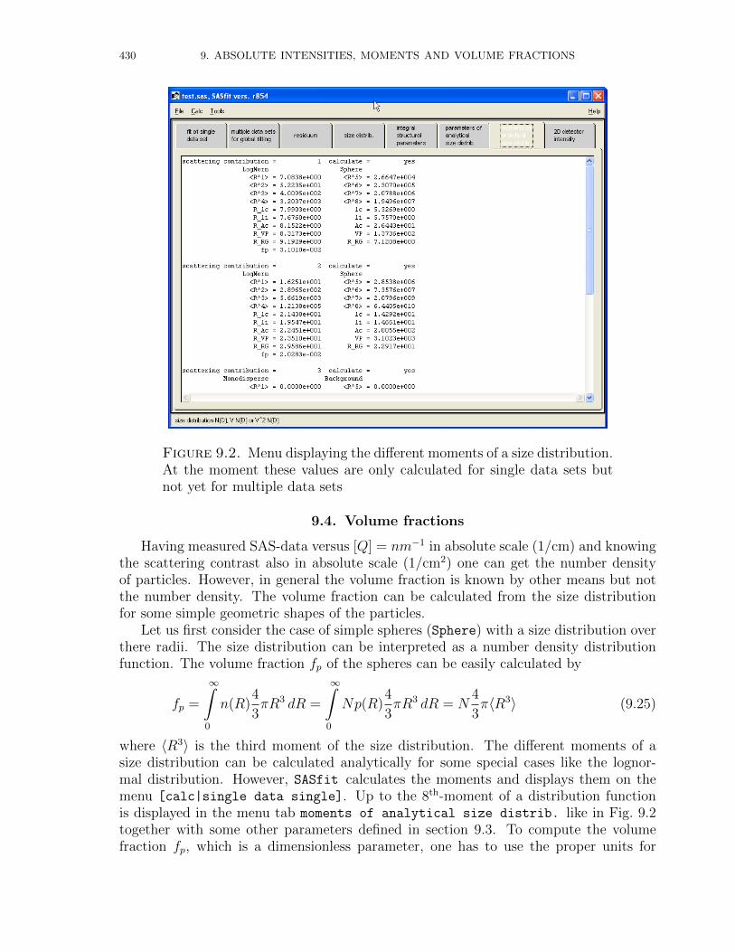
430 9. ABSOLUTE INTENSITIES, MOMENTS AND VOLUME FRACTIONS
Figure 9.2. Menu displaying the different moments of a size distribution.At the moment these values are only calculated for single data sets butnot yet for multiple data sets
9.4. Volume fractions
Having measured SAS-data versus [Q] = nm−1 in absolute scale (1/cm) and knowingthe scattering contrast also in absolute scale (1/cm2) one can get the number densityof particles. However, in general the volume fraction is known by other means but notthe number density. The volume fraction can be calculated from the size distributionfor some simple geometric shapes of the particles.
Let us first consider the case of simple spheres (Sphere) with a size distribution overthere radii. The size distribution can be interpreted as a number density distributionfunction. The volume fraction fp of the spheres can be easily calculated by
fp =
∞∫0
n(R)4
3πR3 dR =
∞∫0
Np(R)4
3πR3 dR = N
4
3π〈R3〉 (9.25)
where 〈R3〉 is the third moment of the size distribution. The different moments of asize distribution can be calculated analytically for some special cases like the lognor-mal distribution. However, SASfit calculates the moments and displays them on themenu [calc|single data single]. Up to the 8th-moment of a distribution functionis displayed in the menu tab moments of analytical size distrib. like in Fig. 9.2together with some other parameters defined in section 9.3. To compute the volumefraction fp, which is a dimensionless parameter, one has to use the proper units for

9.4. VOLUME FRACTIONS 431
N and 〈R3〉. 〈R3〉 has here units of [〈R3〉] = nm3 = 10−21cm3 and N is in unitsof [N ] = 1042cm−3. The volume fraction fp can as an example be computed forN = 8.55241× 10⁻²⁸ and 〈R3〉 = 5.6619× 10³ as
fp = 1042 × 8.55241× 10−28 4
3π 5.6619× 10³ 10−21 = 0.020283. (9.26)
The numbers for N and 〈R3〉 can be directly taken from the SASfit gui.Let us now consider the case of cylinders with a circular cross-section with radius R
and length L. We will have a look on the two cases of having either a distribution inthe radius R or a distribution in the length L. The volume of a cylinder Vcyl is given by
Vcyl(R,L) = πR2L (9.27)
To calculate the volume fraction from the size distribution we need to integrate over theparticle volume. The integration is done either over the radius dR
fp =
∞∫0
n(R)Vcyl(R,L) dR =
∞∫0
Np(R)πR2LdR = NLπ〈R2〉 (9.28)
or over the cylinder length dL
fp =
∞∫0
n(L)Vcyl(R,L) dL =
∞∫0
Np(L)πR2LdL = NR2π〈L〉 (9.29)
depending if we have a distribution over the radius R or the length L. In both cases thevolume fraction can be expressed in terms of moments of the size distribution suppliedby SASfit. In the first case it can be expresses by the second moment 〈R2〉 of thecylinder radius and in the second case by the first moment 〈L〉 of the cylinder length,i.e. the mean cylinder length. The required moments are displayed in SASfit in themenu shown in Fig. 9.2. Also here one has to take care using proper units, but this isdone equivalently to the first example of a sphere in eq. 9.26.
The three examples above show that the volume fraction fp of scatterers can becalculated in many cases via the moments of the size distribution and for simple cases allnecessary parameters are supplied in the SASfit menu interface. The volume fraction fp
in Fig. 9.2 is numerically calculated from the size distribution. For some specific otherform factor and the special case of a LogNorm distribution a plugin size distributionnamed LogNorm fp described in section 8.6 has been implemented. Calculating volumefractions for any size distribution and for any form factor is not easy to implement. Itwould require quite some knowledge about the form factor and how exactly the volumefraction is defined. The plugin LogNorm fp distinguish between volume fraction of a coreonly, a volume fraction of a core together with a shell and a volume fraction of a shell only.For the general case one also needs to know which size parameter of the form factor hasa distribution. This already shows that the user has to supply additional information.For the calculation a volume function has to be associated to each form factor. If thisis not the case the SASfit routine returns 0. For those function a volume function isassociated to the form factor SASfit calculates numerically the volume fraction for anysize distribution by integration. The plugin function LogNorm fp on the other side has alognormal distribution implemented and the information about the form factor and the
432 9. ABSOLUTE INTENSITIES, MOMENTS AND VOLUME FRACTIONS
size parameter of the form factor having a distribution has to be given by the user viaan input value called shape. Only a very limited number of form factor can be selectedby this parameter. For other form factors the plugin needs to be extended or an routinecalculating the volume for the specific form factor needs to be implemented.
CHAPTER 10
Basic Analysis of Dynamic Light Scattering Data
In a typical dynamic light scattering (DLS) or photo correlation scattering (PCS)experiment, the autocorrelation function G(2)(τ) of the intensity scattered by dispersedparticles is determined as a function of the delay τ . G(2)(τ) is related to the modulus ofthe normalized field autocorrelation function g1(τ) by a Siegert relationship
G(2)(τ) = Ag21(τ) +B. (10.1)
Here B is a background term often designated as the baseline and A can be consideredas another instrumental factor. The time dependence of g1(τ) is related to the dynamicsof the dispersed particles. For particles in Brownian motion, the time decay of g1(τ)is determined by the diffusion coefficient of the dispersed particles. In particular, formonodisperse samples g1(τ) is an exponentially decaying function:
g1(τ) = exp(−Γτ) (10.2)
or
G(2)(τ) = A exp(−2Γτ) +B (10.3)
where the decay rate Γ is linked to the particles’ diffusion coefficient D by Γ = DQ2,where Q is the modulus of the scattering vector
Q =4πm1
λ0
sin(θ/2) (10.4)
m1 is the refraction index of the solution, λ0 the wavelength in vacuo of the incident lightand θ the scattering angle. At the end the Stokes-Einstein expression for the diffusioncoefficient is used to get an average particle radius RDLS
D =kT
6πηRDLS
(10.5)
where k is Boltzmann’s constant, T the absolute temperature, η the viscosity of thedispersion medium and RDLS the particle radius (only valid for noninteracting particles).
433
434 10. BASIC ANALYSIS OF DYNAMIC LIGHT SCATTERING DATA
10.1. Cumulant Analysis
The formulas in eq. 10.2 to 10.5 are valid for monodisperse dispersions only. Forpolydisperse dispersions the cumulants method of Koppel (1972) is widely used, whichassumes a multi-exponential behaviour so that g1(τ) and G(2)(τ) can be written in aseries expansion as:
g1(τ) = exp
(−Γ1τ +
Γ2τ2
2− Γ3τ
3
6+ · · ·
)(10.6)
G(2)(τ) = A exp
(−2Γ1τ + Γ2τ
2 − Γ3τ3
3+ · · ·
)+B (10.7)
SASfit assumes for the cumulant fit-routine that the function G(2)(τ) is supplied. Asnormally no error bar is available from the correlator a robust least square procedure isimplemented.
REFERENCE:Dennis E. Koppel, Analysis of Macromolecular Polydispersity in Intensity CorrelationSpectroscopy: The Method of Cumulants, The Journal of Chemical Physics, Vol.1, No.11 (1972), 4815- 4820
10.2. DOUBLE DECAY CUMULANT ANALYSIS 435
10.2. Double Decay Cumulant Analysis
G(2)(τ) = A[p e−2Γa,1 τ+Γa,2 τ2
+ (1− p) e−2Γb,1 τ+Γb,2 τ2]
+B (10.8)
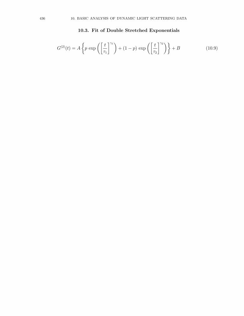
436 10. BASIC ANALYSIS OF DYNAMIC LIGHT SCATTERING DATA
10.3. Fit of Double Stretched Exponentials
G(2)(t) = A
p exp
([t
τ1
]γ1)
+ (1− p) exp
([t
τ2
]γ2)
+B (10.9)

10.3. FIT OF DOUBLE STRETCHED EXPONENTIALS 437
10.3.1. The least squares minimiser and the robust least squares proce-dure. The function to be minimised is
χ2 =∑i
(ri
∆Ii
)2
where the residual is defined asri = Ii − Ii,th.
Here Ii is the intensity correlation function G(2)(ti) at time ti with already subtractedbaseline as received from a correlator, Ii,th is the value of the cumulant fit according toeq. 10.7 or a double exponential decay according to eq. 10.9. Normally no error values∆Ii are supplied from the correlator so that all data points are weighted the same. Arobust fitting with bisquare weights is implemented which uses an iteratively reweightedleast squares algorithm, and follows the procedure:
(1) Fit the model by an unweighted least squares (that is, χ).(2) Standardize the residuals via ui = ri/(Ks). Here K is a tuning constant equal
to 4.685, and s is the robust variance given by MAD/0.6745, where MAD isthe median absolute deviation of the residuals
MAD =N∑i=1
1
N|Ii,th − Ii|
(3) Compute the robust weights wi as a function of the standardized residuals ui.The bisquare weights are given by
wi =
(1− u2
i )2 |ui| < 1
0 |ui| ≥ 1
(4) Re-do the fit using the weighted minimiser:
χ2 =∑i
wi
(ri
∆Ii
)2
(5) The fit converges when the MAD changes by no more than the fraction set byresidual_tolerance (which has been chosen to be 10−8). Otherwise, performthe next iteration of the fitting procedure by returning to the first step.

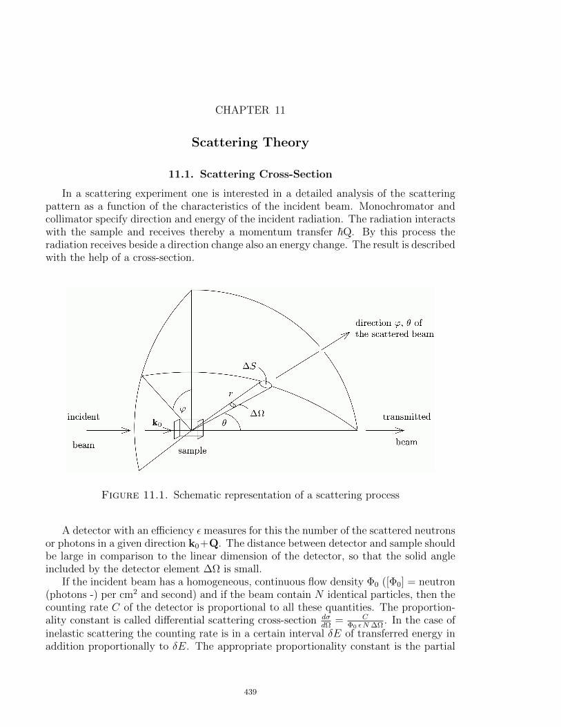
CHAPTER 11
Scattering Theory
11.1. Scattering Cross-Section
In a scattering experiment one is interested in a detailed analysis of the scatteringpattern as a function of the characteristics of the incident beam. Monochromator andcollimator specify direction and energy of the incident radiation. The radiation interactswith the sample and receives thereby a momentum transfer ~Q
¯. By this process the
radiation receives beside a direction change also an energy change. The result is describedwith the help of a cross-section.
Figure 11.1. Schematic representation of a scattering process
A detector with an efficiency ε measures for this the number of the scattered neutronsor photons in a given direction k0+Q. The distance between detector and sample shouldbe large in comparison to the linear dimension of the detector, so that the solid angleincluded by the detector element ∆Ω is small.
If the incident beam has a homogeneous, continuous flow density Φ0 ([Φ0] = neutron(photons -) per cm2 and second) and if the beam contain N identical particles, then thecounting rate C of the detector is proportional to all these quantities. The proportion-ality constant is called differential scattering cross-section dσ
dΩ= C
Φ0 εN ∆Ω. In the case of
inelastic scattering the counting rate is in a certain interval δE of transferred energy inaddition proportionally to δE. The appropriate proportionality constant is the partial
439
440 11. SCATTERING THEORY
(or double) differential scattering cross-section
d2σ
dΩ dE=
C
Φ0 εN ∆Ω ∆E=
Number of neutrons (photons), which are scattered per secondinto the solid angle dΩ toward φ, θ with an energy between Eand E + dE
NΦ0 dΩ dE
The total differential cross-section is defined as
σt = (total number of scattered neutrons (photons) per sec)/Φ0. (11.1)
The three different cross-section are related to each other by
σt =
∫dΩ
dσ
dΩand
dσ
dΩ=
∞∫0
dEd2σ
dΩ dE. (11.2)
11.1.1. Scattering of neutrons on atoms. The scattering of neutrons can beexplained by two types of interactions between neutrons and matter; once the strong spindependent nuclear forces between nuclei and neutron (interaction range ∼ 10−15m) andsecondly the dipole-dipole interaction between the magnetic moment of the neutron andthat of an unpaired electron, or nuclei accordingly. Both interactions have in commonthat their interaction potential V (r
¯) for r → ∞ decays faster than 1/r. For this kind
of interaction potential the quantum mechanical scattering theory [59] yields as anasymptotic approximation for the Schrodinger equation of the wave function
ψk¯0
(r¯) −−−→r→∞
1
(2π)3/2
[eık¯0r¯ + f(θ, φ)
eık0r
r
]. (11.3)
For low energy particles and short range potential the partial waves methods yields forthe scattering amplitude f(θ, φ) = −b, whereby the so called scattering length b can bedetermined experimentally. Via another Ansatz, the Born approximation, one gets aseries expansion for f(θ, φ). The first term of this series expansion is give by
f (0)(θ, φ) = − mN
2π~2
∫dr¯eıQ¯
rV (r¯) , (11.4)
with Q¯
= k¯− k0. A comparison of this result with the partial wave method (f(θ, φ) =
−b), shows that the pseudo potential V (r¯) = 2π~2
mNb δ(r
¯) (Fermi’s pseudo potential) has
an equivalent solution. For an ensemble of N atoms, e.g. a crystal, the total potentialis in kinematic approximation the sum of the individual potentials
V (r¯) =
2π~2
mN
N∑j=1
bjδ(r¯− rj) , (11.5)
whereby r¯j
describes the position of nuclei j with scattering the length bj and N thenumber of scattering atoms. The scattering length bj depends on the element or isotopewhich is the scattering center. Furthermore it can depend on the spin state of theneutron and the nuclei and on unpaired electrons in non fully occupied atomic electronshells. In the kinematic approximation it is assumed that the intensity of the incomingbeam is identical at each scattering center, i.e. that the scattered intensity does notattenuate the incoming beam. Furthermore it is assumed that the incoming beam isonly scattered once and multiple scattered can be neglected.
11.1. SCATTERING CROSS-SECTION 441
In the static approximation, i.e. for a scattering process which does not change thestate of the scattering center and therefore is an elastic scattering process, the differentialscattering cross-section can be described in terms of a scattering amplitude f (0)(θ, φ) by
dσ
dΩ(Q¯
) =1
N
∣∣f (0)(θ, φ)∣∣2 =
1
N
( mN
2π~2
)2∣∣∣∣∫ dr
¯eıQ¯
r V (r¯)
∣∣∣∣2 . (11.6)
Using Fermi’s pseudo potentials (eq. 11.5) leads to the expression
dσ
dΩ(Q¯
) =1
N
∣∣∣∣∣N∑j=1
bj eıQ¯rj
∣∣∣∣∣2
=1
N
∑i,j
bi bj eıQ¯ri e−ıQ
¯rj (11.7)
Let us now consider a new system of scatterers, which are only different to thosefrom eq. 11.7 that the scattering length of the nuclei are exchanged. Hereby both theposition and fraction of the scattering length bi are kept the same. For a large number ofscattering centers the average over the cross-sections of all possible systems of scattererswhich are identical to the one in 11.7 can be described by
dσ
dΩ(Q¯
) =1
N
∑i,j
bi bj eıQ¯ri e−ıQ
¯rj . (11.8)
If the scattering length bi occur in the same fraction xi, whereby∑
i xi = 1, so that the
averages b and b2 can be written as
b =∑i
xi bi and b2 =∑i
xib2i . (11.9)
Under the condition that there are no correlations between the scattering lengths of theindividual nuclei one can write
bi bj = b2
for i 6= j and bi bj = b2 for i = j (11.10)
From this it follows for the differential cross-section
dσ
dΩ(Q¯
) =1
N
b2 + b2∑
i,ji 6=j
eıQ¯ri e−ıQ
¯rj
=1
N
(b2 − b2
)︸ ︷︷ ︸
dσincdΩ
+1
Nb
2
∣∣∣∣∣∑i
eıQ¯ri
∣∣∣∣∣2
︸ ︷︷ ︸dσcohdΩ
(11.11)
11.1.1.1. Nuclear scattering. The simplest system of scatterers consist of only oneisotope with nuclear spin I. As the spin of the neutron is s = ±1/2 only two orientationsare possible: parallel spins of neutron and nuclei, i.e. a total spin of J(+) = I + 1/2 orantiparallel spins, i.e J(−) = I − 1/2. The corresponding scattering length are namedb(+) and b(−).
1
The number of possible states for the total spin J(±) are 2J(+) + 1 = 2I + 2 and2J(−) + 1 = 2I. In case of unpolarized neutrons and/or random oriented nuclear spins
1For coherent scattering the spin of the neutrons keep constant in contrast to incoherent scatteringwhere a part come along with a spin-flip. This can e.g. be used to change the ration between coherentand incoherent scattering.
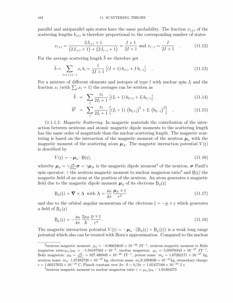
442 11. SCATTERING THEORY
parallel and antiparallel spin states have the same probability. The fraction x(±) of thescattering lengths b(±) is therefore proportional to the corresponding number of states
x(+) =2J(+) + 1(
2J(+) + 1)
+(2J(−) + 1
) =I + 1
2I + 1and x(−) =
I
2I + 1. (11.12)
For the average scattering length b we therefore get
b =∑
i=(+),(−)
xi bi =1
2I + 1
[(I + 1) b(+) + I b(−)
]. (11.13)
For a mixture of different elements and isotopes of type l with nuclear spin Il and thefraction xl (with
∑l xl = 1) the averages can be written as
b =∑l
xl2Il + 1
[(Il + 1) bl(+) + Il bl(−)
](11.14)
b2 =∑l
xl2Il + 1
[(Il + 1)
(bl(+)
)2+ Il
(bl(−)
)2]
. (11.15)
11.1.1.2. Magnetic Scattering. In magnetic materials the contribution of the inter-action between neutrons and atomic magnetic dipole moments to the scattering lengthhas the same order of magnitude than the nuclear scattering length. The magnetic scat-tering is based on the interaction of the magnetic moment of the neutron µn with themagnetic moment of the scattering atom µA. The magnetic interaction potential V (r
¯)
is described by
V (r¯) = −µn · B¯(r
¯), (11.16)
whereby µn = γ e~2mpσ = γµN is the magnetic dipole moment2 of the neutron, σ Pauli’s
spin operator, γ the neutron magnetic moment to nuclear magneton ratio3 and B¯
(r¯) the
magnetic field of an atom at the position of the neutron. An atom generates a magneticfield due to the magnetic dipole moment µS of its electrons B
¯S(r¯)
B¯S
(r¯) = ∇× A
¯with A
¯=µ0
4π
µS × r¯
r3(11.17)
and due to the orbital angular momentum of the electrons l¯
= −p¯× r
¯which generates
a field of B¯L
(r¯)
B¯L
(r¯) = −µ0
4π
2µB~
p¯× r
¯r3
. (11.18)
The magnetic interaction potential V (r¯) = −µn · (B¯S(r
¯) + B
¯L(r¯)) is a weak long range
potential which also can be treated with Born’s approximation. Compared to the nuclear
2neutron magnetic moment: µn = −0.96623645× 10⁻²⁶ JT−1, neutron magnetic moment to Bohrmagneton ratio:µn/µB = −1.04187563 × 10⁻³, nuclear magneton: µn = 5.05078343 × 10⁻²⁷ JT−1,Bohr magneton: µB = e~
2me= 927.400949 × 10⁻²⁶ JT−1, proton mass: mp = 1.67262171 × 10⁻²⁷ kg,
neutron mass: mn: 1.67492728× 10⁻²⁷ kg, electron mass: me9.1093826× 10−31kg, elementary charge:e = 1.60217653× 10⁻¹⁹ C, Planck constant over 2π: ~ = h/2π = 1.05457168× 10⁻³⁴ J s
3neutron magnetic moment to nuclear magneton ratio γ = µn/µN − 1.91304273
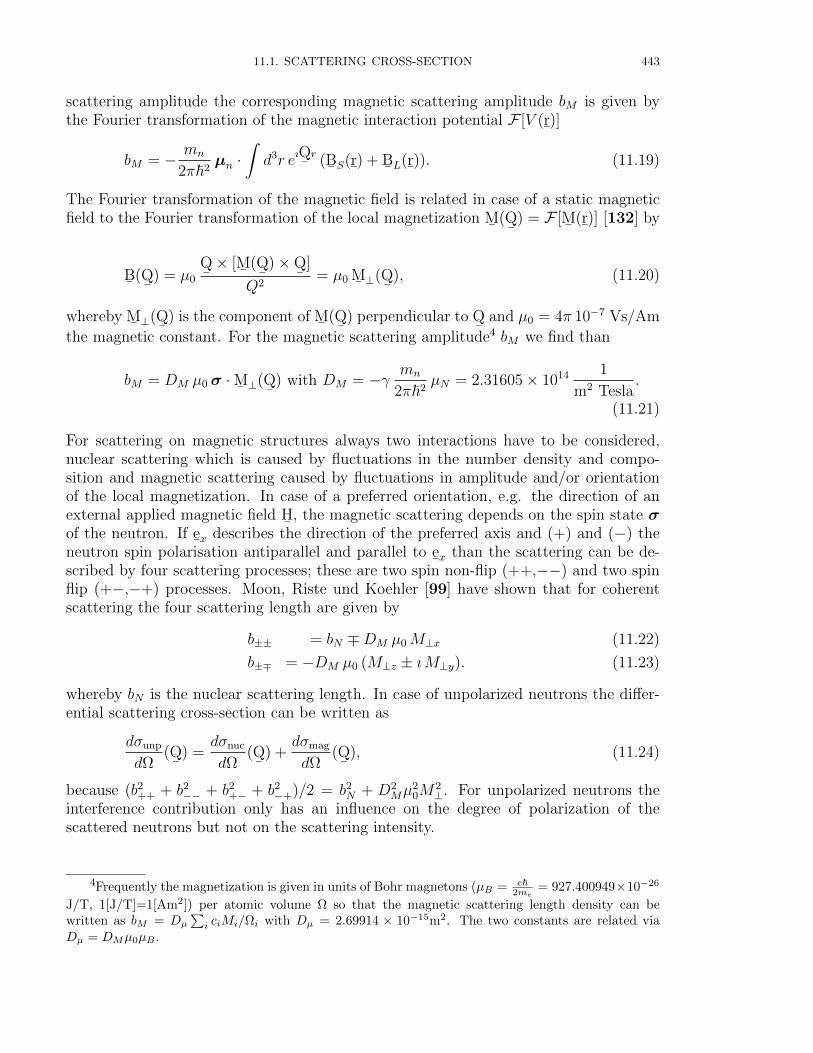
11.1. SCATTERING CROSS-SECTION 443
scattering amplitude the corresponding magnetic scattering amplitude bM is given bythe Fourier transformation of the magnetic interaction potential F [V (r
¯)]
bM = − mn
2π~2µn ·
∫d3r eıQ¯
r (B¯S
(r¯) + B
¯L(r¯)). (11.19)
The Fourier transformation of the magnetic field is related in case of a static magneticfield to the Fourier transformation of the local magnetization M
¯(Q¯
) = F [M¯
(r¯)] [132] by
B¯
(Q¯
) = µ0
Q¯× [M
¯(Q¯
)×Q¯
]
Q2= µ0 M
¯ ⊥(Q¯
), (11.20)
whereby M¯ ⊥
(Q¯
) is the component of M¯
(Q¯
) perpendicular to Q¯
and µ0 = 4π 10−7 Vs/Am
the magnetic constant. For the magnetic scattering amplitude4 bM we find than
bM = DM µ0 σ ·M¯ ⊥
(Q¯
) with DM = −γ mn
2π~2µN = 2.31605× 10¹⁴ 1
m2 Tesla.
(11.21)
For scattering on magnetic structures always two interactions have to be considered,nuclear scattering which is caused by fluctuations in the number density and compo-sition and magnetic scattering caused by fluctuations in amplitude and/or orientationof the local magnetization. In case of a preferred orientation, e.g. the direction of anexternal applied magnetic field H
¯, the magnetic scattering depends on the spin state σ
of the neutron. If e¯x
describes the direction of the preferred axis and (+) and (−) theneutron spin polarisation antiparallel and parallel to e
¯xthan the scattering can be de-
scribed by four scattering processes; these are two spin non-flip (++,−−) and two spinflip (+−,−+) processes. Moon, Riste und Koehler [99] have shown that for coherentscattering the four scattering length are given by
b±± = bN ∓DM µ0M⊥x (11.22)
b±∓ = −DM µ0 (M⊥z ± ıM⊥y). (11.23)
whereby bN is the nuclear scattering length. In case of unpolarized neutrons the differ-ential scattering cross-section can be written as
dσunp
dΩ(Q¯
) =dσnuc
dΩ(Q¯
) +dσmag
dΩ(Q¯
), (11.24)
because (b2++ + b2
−− + b2+− + b2
−+)/2 = b2N + D2
Mµ20M
2⊥. For unpolarized neutrons the
interference contribution only has an influence on the degree of polarization of thescattered neutrons but not on the scattering intensity.
4Frequently the magnetization is given in units of Bohr magnetons (µB = e~2me
= 927.400949×10⁻²⁶
J/T, 1[J/T]=1[Am2]) per atomic volume Ω so that the magnetic scattering length density can bewritten as bM = Dµ
∑i ciMi/Ωi with Dµ = 2.69914 × 10⁻¹⁵m2. The two constants are related via
Dµ = DMµ0µB .
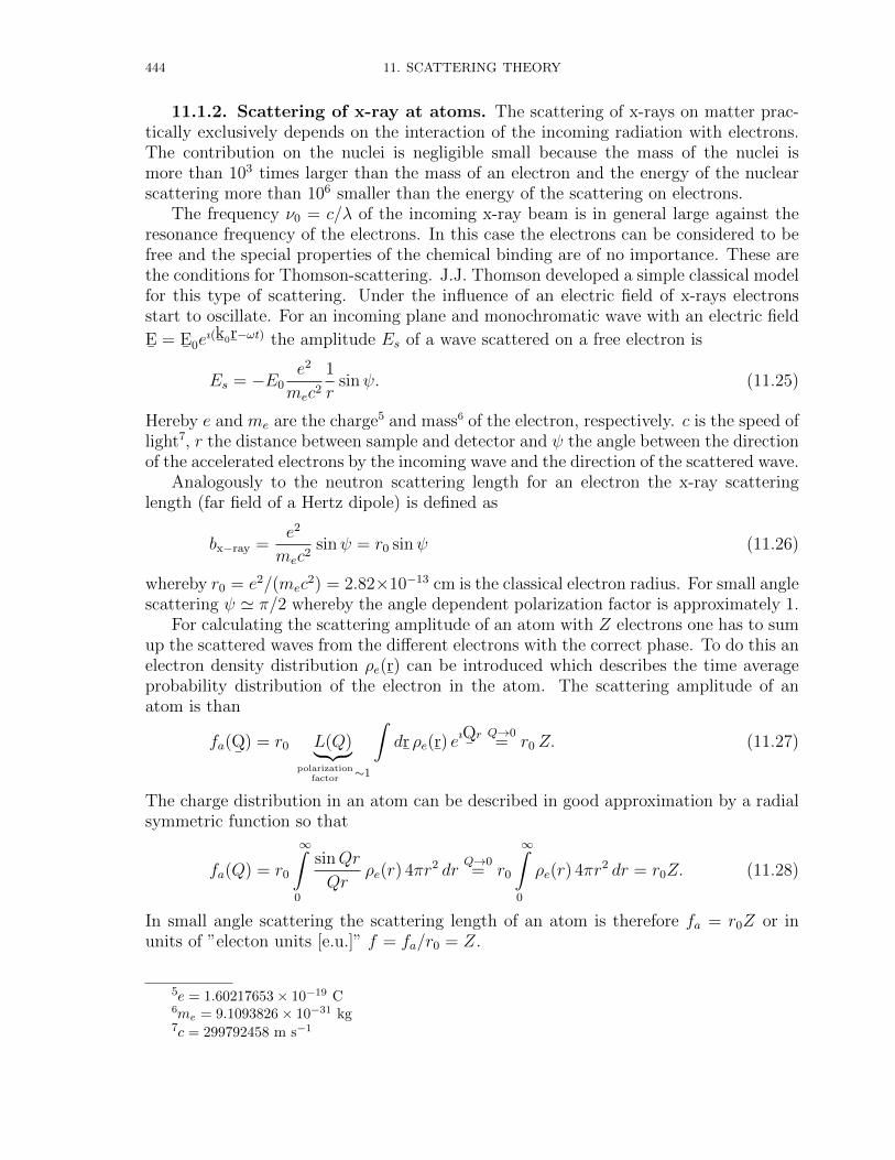
444 11. SCATTERING THEORY
11.1.2. Scattering of x-ray at atoms. The scattering of x-rays on matter prac-tically exclusively depends on the interaction of the incoming radiation with electrons.The contribution on the nuclei is negligible small because the mass of the nuclei ismore than 103 times larger than the mass of an electron and the energy of the nuclearscattering more than 106 smaller than the energy of the scattering on electrons.
The frequency ν0 = c/λ of the incoming x-ray beam is in general large against theresonance frequency of the electrons. In this case the electrons can be considered to befree and the special properties of the chemical binding are of no importance. These arethe conditions for Thomson-scattering. J.J. Thomson developed a simple classical modelfor this type of scattering. Under the influence of an electric field of x-rays electronsstart to oscillate. For an incoming plane and monochromatic wave with an electric field
E¯
= E¯0e
ı(k¯0r¯−ωt) the amplitude Es of a wave scattered on a free electron is
Es = −E0e2
mec2
1
rsinψ. (11.25)
Hereby e and me are the charge5 and mass6 of the electron, respectively. c is the speed oflight7, r the distance between sample and detector and ψ the angle between the directionof the accelerated electrons by the incoming wave and the direction of the scattered wave.
Analogously to the neutron scattering length for an electron the x-ray scatteringlength (far field of a Hertz dipole) is defined as
bx−ray =e2
mec2sinψ = r0 sinψ (11.26)
whereby r0 = e2/(mec2) = 2.82×10⁻¹³ cm is the classical electron radius. For small angle
scattering ψ ' π/2 whereby the angle dependent polarization factor is approximately 1.For calculating the scattering amplitude of an atom with Z electrons one has to sum
up the scattered waves from the different electrons with the correct phase. To do this anelectron density distribution ρe(r
¯) can be introduced which describes the time average
probability distribution of the electron in the atom. The scattering amplitude of anatom is than
fa(Q¯
) = r0 L(Q)︸ ︷︷ ︸polarization
factor∼1
∫dr¯ρe(r
¯) eıQ¯
r Q→0= r0 Z. (11.27)
The charge distribution in an atom can be described in good approximation by a radialsymmetric function so that
fa(Q) = r0
∞∫0
sinQr
Qrρe(r) 4πr2 dr
Q→0= r0
∞∫0
ρe(r) 4πr2 dr = r0Z. (11.28)
In small angle scattering the scattering length of an atom is therefore fa = r0Z or inunits of ”electon units [e.u.]” f = fa/r0 = Z.
5e = 1.60217653× 10⁻¹⁹ C6me = 9.1093826× 10⁻³¹ kg7c = 299792458 m s−1
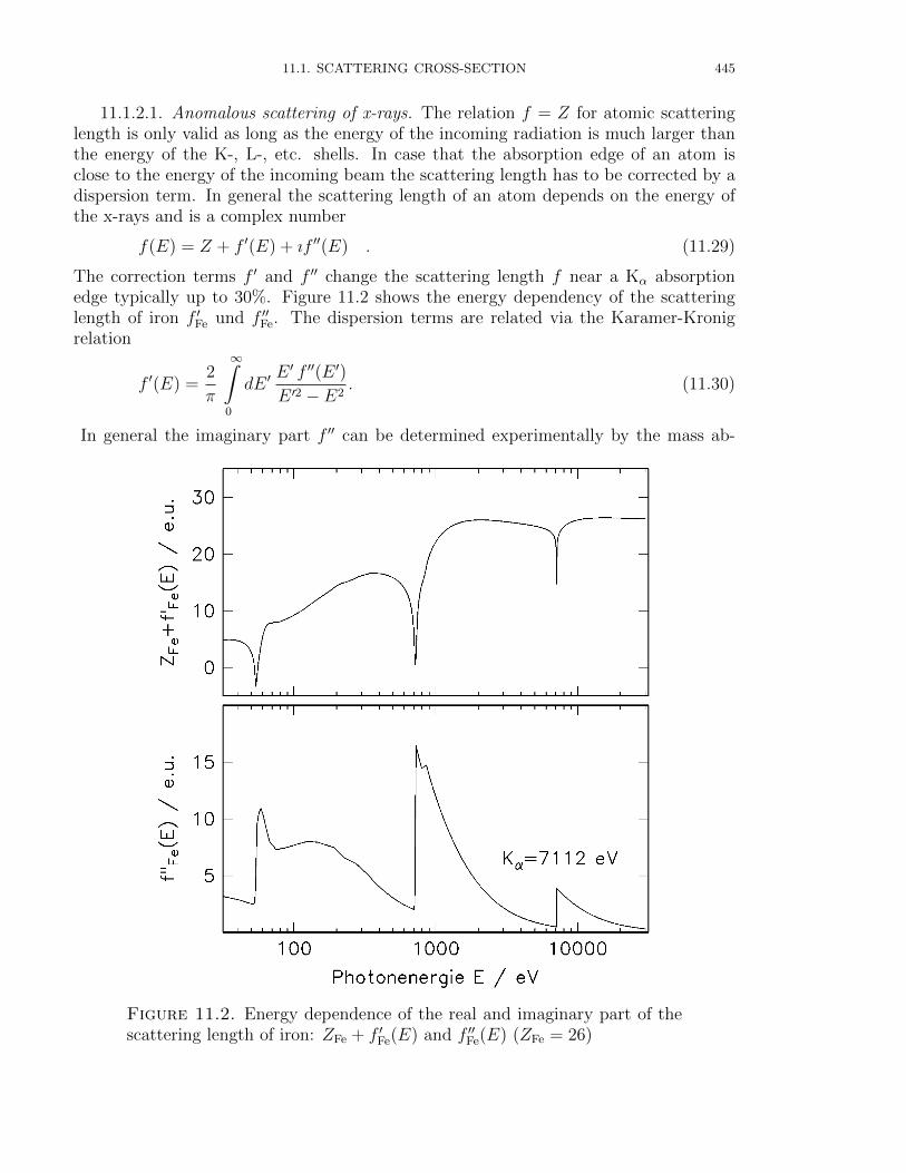
11.1. SCATTERING CROSS-SECTION 445
11.1.2.1. Anomalous scattering of x-rays. The relation f = Z for atomic scatteringlength is only valid as long as the energy of the incoming radiation is much larger thanthe energy of the K-, L-, etc. shells. In case that the absorption edge of an atom isclose to the energy of the incoming beam the scattering length has to be corrected by adispersion term. In general the scattering length of an atom depends on the energy ofthe x-rays and is a complex number
f(E) = Z + f ′(E) + ıf ′′(E) . (11.29)
The correction terms f ′ and f ′′ change the scattering length f near a Kα absorptionedge typically up to 30%. Figure 11.2 shows the energy dependency of the scatteringlength of iron f ′Fe und f ′′Fe. The dispersion terms are related via the Karamer-Kronigrelation
f ′(E) =2
π
∞∫0
dE ′E ′ f ′′(E ′)
E ′2 − E2. (11.30)
In general the imaginary part f ′′ can be determined experimentally by the mass ab-
Figure 11.2. Energy dependence of the real and imaginary part of thescattering length of iron: ZFe + f ′Fe(E) and f ′′Fe(E) (ZFe = 26)
446 11. SCATTERING THEORY
sorption coefficient µm(E) = 2NAAλ r0 f
′′(E) (Na Avogadro number, A mass of atom inresonance) to calculate than with equation 11.30 the real part of the scattering lengthf ′(E).
11.2. Small angle scattering
In small angle scattering geometry the structural unit down to single atoms cannot be resolved, only structures larger than several atomic layers can be seen by thatmethod. Small angle scattering techniques measure the beam scattered close to forwarddirection whereby the beam divergence is in the order λ/L 1. For a wavelength ofλ = 1 nm and a characteristic dimension L = V 1/3 of the scatterer of about 10 nm thedivergency of the beam is about λ/L = 0.1 rad ' 6.3.
In principle with small angle scattering both information on size as well as shapeof the scatterer and information on the relative arrangement of the scatterer can beobtained. In the following an overview of the theoretical basics to analyze small anglescattering data will be given.
In section 11.1 the scattering of an ensemble of atoms has been discussed. Thereinterference terms between the waves scattered by the individual atoms were importantfor the differential scattering cross-section (eq. 11.7 ,11.28).
dσ
dΩ(Q¯
) =1
N
∣∣∣∣∣N∑j=1
bj eıQ¯rj
∣∣∣∣∣2
ordσ
dΩ(Q¯
) =1
N
∣∣∣∣∣N∑j=1
fa,j(Q¯
) eıQ¯r
∣∣∣∣∣2
. (11.31)
Small angle scattering normally does not resolve dimension down to atomic dimensions.Therefore the summation over the individual atoms can be replaced by an integrationover the illuminated volume V :
dσ
dΩ(Q¯
) =1
N
∣∣∣∣∣∣∫V
dr¯ρ(r
¯) eıQ¯
r
∣∣∣∣∣∣2
=1
NI(Q
¯) , (11.32)
whereby ρ(r¯) is the local scattering length density and F (Q
¯) the scattering amplitude.
The differential scattering cross-section is mathematically the square of the modulusof the Fourier transformation of the scattering length density. The scattering lengthdensity ρ(r
¯) is proportional to the locally averaged scattering potential V (r
¯). Thats why
equation 11.32 is except a constant identical to equation 11.6. The scattering intensityI(Q
¯) = |z|2 = z z∗ can therefore be written as
I(Q¯
) =
∫∫dr¯1 dr
¯2 ρ(r¯1) ρ∗(r
¯2) eıQ¯(r1−r2) . (11.33)
By using the substitution r¯
= r¯1 − r
¯2 one get
I(Q¯
) =
∫dr¯eıQ¯
r
∫dr¯1 ρ(r
¯1) ρ∗(r¯1 − r
¯)︸ ︷︷ ︸
Γ(r¯) = ρ(r
¯) ~ ρ(r
¯)
=
∫dr¯
Γ(r¯) eıQ¯
r . (11.34)
11.2. SMALL ANGLE SCATTERING 447
Γ(r¯) is the autocorrelation function8 In case of a real scattering length density eq. 11.34
is the convolution integral Γ(r¯) = ρ(r
¯) ∗ ρ(r
¯) =
∫dr¯1 ρ(r
¯1) ρ(r¯1 − r
¯) of the scattering
length density and is called Patterson function9.
11.2.1. Autocorrelation function Γ(r¯) and γ(r
¯). In the following we will make
use of two simplifications. Firstly the scattering system is assumed to be isotropic.Hereby the isotropy can have its origin both in the shape of the scatterer or being aconsequence of the temporal change of the particle orientation. The consequence is that
Γ(r¯) only depends on the modulus of r and eıQ¯
r can be averaged over all orientations ofr¯. (The second simplification will follow further below)
11.2.1.1. Isotropic averages. If α is assigned to the angle between Q¯
and r¯
and if allorientations α are equal probable than the probability pα dα that Q
¯and r
¯include the
angle α is equal to 12
sinα dα.
pα dα =2π R sinα
4π R2Rdα =
sinα
2dα (11.35)
The average of eıQ¯r over all orientations of r
¯is
eıQ¯r
r¯ =
π∫0
dαsinα
2eıQr cosα =
sinQr
Qr(11.36)
=
π∫0
dαsinα
2cos(Qr cosα)
︸ ︷︷ ︸symmetric to α=π/2
+ı
π∫0
dαsinα
2sin(Qr cosα)
︸ ︷︷ ︸antisymmetric to α=π/2 ⇒ =0
= 2
π2∫
0
dαsinα
2cos(Qr cosα) =
1
Qr
Qr∫0
du cosu =sinQr
Qr
and equation 11.34 is simplified to
I(Q) =
∫dr 4π r2 Γ(r)
sinQr
Qr. (11.37)
8Normally the autocorrelation function is defined as ρ(r¯) ~ ρ(r
¯) =
∫dr¯1ρ(r
¯1) ρ∗(r
¯1+ r
¯), so that in
fact Γ(r¯) should be Γ(r
¯) = ρ(−r
¯) ~ ρ(−r
¯).
9Here the Patterson function is defined as the autocorrelation of the scattering length density ρ(r¯).
Instead of defining the cross-section via a scattering length density as in 11.34 in neutron scatteringthe differential cross-section is often defined as dσcoh(Q
¯)/dΩ = (σcoh/4πN)
∫dr¯ρ(r
¯) ~ ρ(r
¯) exp(ıQ
¯r¯),
whereby σcoh = 4π b2
is the coherent cross-section and ρ(r¯) the particle number density. The Patterson
function is than the autocorrelation of the particle number density. This function is independent ofthe scattering lengths and only dependent on the geometric arrangement of the scattering centers.The Fourier transformation of the Patterson function is therefore sometimes called Structure factorS(Q
¯) and is related in case of a static approximation to the differential cross-section by the equation
dσcoh(Q¯
)/dΩ = (σcoh/4πN)S(Q¯
).
448 11. SCATTERING THEORY
11.2.1.2. Absence of long range order. As a second simplification it will be assumedthat long range order is absent. The consequence is that the autocorrelation Γ(r) be-comes constant for large values of r. It converges to Γ = ρ2V . ρ is the average scatteringlength density defined by∫
dr¯
(ρ(r¯)− ρ) =
∫dr¯η(r
¯) = 0 . (11.38)
Structural information is therefore only contained in a finite range of Γ(r¯) where it
deviates from the average value Γ. This is due to the fact that only a deviation of η(r¯)
from the average ρ leads to a scattering contribution for Q 6= 0. An additional constantvalue ρ only contributes to the scattering at Q = 0 and is therefore not accessible.Consequently the average scattering length density can be subtracted without loss ofgenerality and only deviations η(r
¯) = ρ(r
¯)−ρ have to be considered. The autocorrelation
function is therefore defined as
γ(r) =1
Vη(r
¯) ~ η(r
¯)
r¯ =
1
V(ρ(r
¯)− ρ) ~ (ρ(r
¯)− ρ)
r¯ (11.39)
⇒ I(Q) = V
∞∫0
dr 4π r2 γ(r)sinQr
Qr. (11.40)
V γ(r¯) is different from Γ(r
¯) due to the definition of ρ (eq. 11.38) only by a constant
term ρ2 V , i.e. V γ(r¯) = Γ(r
¯)− ρ2 V because
Γ(r¯) =
∫dr¯1 ρ(r
¯1) ρ∗(r¯1 − r
¯) =
∫dr¯1 (ρ+ η(r
¯1))(ρ+ η(r¯1 − r
¯))∗ (11.41)
= ρ2V +
∫dr¯1 (ρ η(r
¯1) + ρ∗ η∗(r¯1 − r
¯))︸ ︷︷ ︸
= 0 due to def. of η(r¯) in eq. 11.38
+
∫dr¯1 η(r
¯1) η∗(r¯1 − r
¯)(11.42)
= ρ2V + γ(r¯)V. (11.43)
11.2.1.3. Limits r = 0 and r =∞. The limits r = 0 and r →∞ for the autocorrela-tion γ(r
¯) are γ(0) = η2 and γ(∞) = 0. The limit r →∞ is zero because η(r
¯) is defined
as the deviation of the average scattering length density ρ. As long range correlation isassumed not to be present η(r
¯)~ η(r
¯)r→∞= η2 = 0. γ(r) can be calculated by the inverse
Fourier transformation of the scattering intensity I(Q) (eq. 11.40)
V γ(r) =1
2π2
∞∫0
dQQ2 I(Q)sinQr
Qr. (11.44)
An important special case is r = 0 for which equation 11.44 can be simplified to
V γ(0) = V η2 =1
2π2
∞∫0
dQQ2 I(Q) =Q
2π2. (11.45)
The integration of the intensity I(Q) in reciprocal space is therefore directly related to
the average quadratic deviation of the scattering length density η2 but independent tothe shape of the scatterers. If for example the scattering particle undergoes deformation
11.2. SMALL ANGLE SCATTERING 449
the scattering pattern may change drastically but the integral Q in eq. 11.45 keepsinvariant against such a deformation.
11.2.2. Volume fraction. The average quadratic deviation of the scattering lengthdensity is directly related in a two-phase system to the scattering contrast ∆η and volumefraction fp of one or the other (1 − fp) phase. The average quadratic deviation of thescattering length density is defined as
η2 = η21 fp + η2
2 (1− fp), (11.46)
whereby η1 and η2 are the scattering length density differences of the two phases fromthe average value ρ and the scattering contrast is than defined as ∆η = η1 + η2. Theaverage value ρ is given by
ρ = (ρ− η1)fp + (ρ+ η2)(1− fp) ⇔ fp (η1 + η2) = fp ∆η = η2 (11.47)
or (1− fp) ∆η = η1 .
Replacing η1 and η2 in eq. 11.46 leads to
η2 = ∆η2 fp(1− fp). (11.48)
The second moment of the scattering intensity, the so-called scattering invariant Q fromeq. 11.45, can therefore be related to the volume fractions of the two phases fp and(1− fp) by
Q =
∫dQQ2 I(Q) = 2π2 V ∆η2 fp(1− fp) . (11.49)
Due to the Babinet principle in a scattering experiment the volume fractions can notbe uniquely assigned to one or the other phase. A system with exchanged phases wouldhave the same invariant A unique solution of eq. 11.49 for the volume fraction can onlybe obtained if either one already knows from somewhere else that the volume fraction ofone phase is much smaller than the volume fraction of the other (dilute case) or if timeresolved experiments are performed during the formation of the structure and when itis known that one phase is growing on the cost of the other one (Ostwald ripening).
11.2.3. Interparticle interferences. The square of the Fourier transformation ofthe scattering length density of a sample with a volume V is equal to the scatteringintensity I(Q
¯)
I(Q¯
) =
∣∣∣∣∣∣∫V
dr¯ρ(r
¯) eıQ¯
r
∣∣∣∣∣∣2
. (11.50)
The integration has to be carried out over the whole illuminated sample volume V . Ifthe sample volume contains N particles embedded in a matrix with a constant scatteringlength density ρM and if R
¯ idefines the center of particle i with a constant scattering

450 11. SCATTERING THEORY
length density ρP,i = ∆ηi + ρM the scattering intensity can be written as
I(Q¯
) =
∣∣∣∣∣N∑i=1
Fi(Q¯
) eıQ¯Ri
∣∣∣∣∣2
(11.51)
with Fi(Q¯
) =
∫Vi(R
¯ i)
dr¯
∆ηi eıQ¯
(r¯−Ri) = ∆ηi
∫Vi(0
¯)
dr¯eıQ¯
r = ∆ηi Vi fi(Q¯
).
Vi(R¯ i
) describes the integration volume of scatterer i located at R¯ i
and Vi(0¯) describes
the integration volume of the scatterer i moved to the origin of the coordinate system.∆ηi and Vi are the scattering contrast and particle volume, respectively. The square ofthe modulus in eq. 11.51 can be rewritten to
I(Q¯
) =N∑i=1
N∑j=1
Fi(Q¯
)F ∗j (Q¯
) eıQ¯R¯ ij
=N∑i=1
∣∣Fi(Q¯
)∣∣2 + (11.52)
2N∑i=1
N∑j>i
[<(Fi(Q
¯)F ∗j (Q
¯))
cos Q¯
R¯ ij−=
(Fi(Q
¯)F ∗j (Q
¯))
sin Q¯
R¯ ij]
︸ ︷︷ ︸Ψ(Q
¯)
The first term for which i = j the phase factor is identical to 1 and describes thesum of the scattering intensity of individual particles. The double sum in the secondterm describes interference effects of the scattering amplitudes scattered from differentparticles which depends on their relative arrangement R
¯ ij= R
¯ i− R
¯ j. The scattering
amplitude Fi(Q¯
) is among other things dependent on the scattering contrast ∆ηi and onthe normalized form factor Fi(Q
¯)/∆ηiVi = fi(Q
¯), whereby fi(Q
¯) is a real-valued function
with fi(Q = 0) = 1. Analytical expressions for scattering intensities i0(Q) = |f(Q)|2 ofsimple geometric bodies are listed in the chapter 3. In case ∆ηi is complex valued, i.e.the scatterer has an absorption contrast ∆η′′i , the scattering contrast can be written as∆ηi = ∆η′i + ı∆η′′i and for the interference term we get
Ψ(Q¯
) = 2N∑i=1
N∑j>i
fi(Q¯
) fj(Q¯
)Vi Vj (11.53)
×[(∆η′i ∆η
′j + ∆η′′i ∆η′′j ) cos Q
¯R¯ ij− (∆η′i ∆η
′′j −∆η′′i ∆η′j) sin Q
¯R¯ ij]
.
11.2. SMALL ANGLE SCATTERING 451
If now all particle have an identical scattering contrast ∆η = ∆ηi = ∆ηj we get for thescattering intensity (eq. 11.51) the expression
I(Q¯
) =N∑i=1
V 2i (∆η′2 + ∆η′′2)
∣∣fi(Q¯
)∣∣2
+2N∑i=1
N∑j>i
fi(Q¯
) fj(Q¯
)Vi Vj (∆η′2 + ∆η′′2) cos Q¯
R¯ ij
. (11.54)
For identical scattering contrasts there is consequently no interference between the scat-tering amplitude of waves scattered at the real and at the imaginary (absorption) partof the scattering contrast.
11.2.3.1. Isotropic ensemble of particles. In the following we assume as another sim-plification an isotropic ensemble of particles. Such a system of scatterer is defined asfollows: If R
¯ idefines the position of any particle i and R
¯ ijis the difference vector be-
tween the position of particle i and j than a system of particles is called isotropic if allvectors R
¯ ijof the same length will take with equal probability any direction. Under this
simplification the interference term Ψ(Q¯
) in eq. 11.53 can be averaged over all directions
R¯ ij
. This average yield for sin Q¯Rij
R¯ ij = 0 and for cos Q
¯Rij
R¯ ij =
sinQRijQRij
(compare
with eq. 11.37). The interference term can then be written as
Ψ(Q¯
) = 2N∑i=1
N∑j>i
fi(Q¯
) fj(Q¯
)Vi Vj (∆η′i ∆η′j + ∆η′′i ∆η′′j )
sinQRij
QRij
. (11.55)
Therefore also for an isotropic ensemble of scatterers no interferences between wavesscatterer at the real and imaginary part of the scattering contrast disappears as alreadyshown for systems of particles with identical scattering contrast.
11.2.4. Influence of the relative arrangement of scatterers on interparti-cle interferences. The expression for Ψ(Q
¯) can be further simplified if the scattering
system consist of identical particles which fulfill the condition that for all of them eachorientation be likewise probable and furthermore the relative position of two particlesdo not have an influence on their orientation. The second part of the assumption isfor radial symmetric particle automatically fulfilled. However, in case of a system ofclose packed ellipsoidal particles with half axis R, R and νR with ν > 1 distance of 2Rbetween the centers of the ellipsoids are possible, but for such an arrangement not allorientations of the ellipsoids are allowed anymore. That means that the relative distancehas an influence on allowed orientations of the particles. The general case without therestrictions made in this paragraph are discussed by Guinier and Fournet in [50]. Foronly slightly anisotropic and not to closely packed systems the assumptions made hereare at least fulfilled in first approximation. Under the made assumptions the averag-ing over the particle orientations can be separated from the averaging of the particlepositions. As a result from the average one gets for the scattering intensity
I(Q) = N |F (Q)|2 + 2∣∣∣F (Q)
∣∣∣2 N∑i=1
N∑j>i
sinQRij
QRij
(11.56)

452 11. SCATTERING THEORY
For low concentrations this averaging is in first approximation also valid for particleswith a size distribution. The probability to find a particle at the position R
¯ iis in average
NVdR
¯ iand the probability to find at the same time another particle at position R
¯ jis
NVdR
¯ iNVdR
¯ j. A deviation from this is considered by P (Rij) so that the double sum in
eq. 11.56 can be written as
N∑i=1
N∑j>i
sinQRij
QRij
=
∫V
∫V
sinQRij
QRij
P (Rij)N2
V 2dR
¯ idR
¯ j. (11.57)
For isotropic media the function P (Rij) is independent of the indices i and j and only afunction of the distance R. P (R) has the property to converge for large distance againstone. By the substitution P (R) = 1− (1− P (R)) one gets for the interference term
Ψ(Q) =∣∣∣F (Q)
∣∣∣2N2
V 2
∫V
∫V
sinQRij
QRij
dR¯ idR
¯ j(11.58)
−∣∣∣F (Q)
∣∣∣2N2
V 2
∫V
∫V
sinQRij
QRij
(1− P (Rij)) dR¯ idR
¯ j. (11.59)
The first term can be interpreted as the scattering of a particle with the volume V andthe average scattering contrast F (Q)N
V. As the illuminated sample volume V is relatively
large this contribution is practically zero for all experimental accessible scattering angles.As for isotropic media the integration over dR
¯ iis independent from the integration over
dR¯ j
and (1 − P (R)) quickly converges against zero the first integrationin the secondterm (neglecting side effects) can be written as
∞∫0
dRsinQR
QR(1− P (R))
N2
V 24 π R2. (11.60)
The second integration only yields an additional multiplication factor V . Finally onegets for the scattering intensity the expression
I(Q) = N
|F (Q)|2 −∣∣∣F (Q)
∣∣∣2 NV
∫dR 4π R2 (1− P (R))
sinQR
QR︸ ︷︷ ︸Υ(Q)
.
(11.61)
11.2.4.1. Formula from Prins and Zernicke. For radial symmetric identical scatterer
the quare of the average form factor∣∣∣F (Q)
∣∣∣2 and the average of the squared form factor
|F (Q)|2 are the same so that one get for the expression from Prins and Zernicke [157]and from Debye und Mencke [31]
I(Q) = N F 2(Q)
1− N
V
∫dR 4π R2 (1− P (R))
sinQR
QR
︸ ︷︷ ︸
S(Q)=1−Υ(Q)
. (11.62)
11.2. SMALL ANGLE SCATTERING 453
The problem of applying eq. 11.61 or 11.62 is the evaluation of P (R). P (R) depends onthe geometric arrangement of the scatterer. For liquid emulsions the geometric arrange-ment can be related to thermodynamic quantities like concentration, temperature andinteraction potential between the particles. In a theory of Raman [119] the geometricarrangement is associated to the interaction potential U(r) in a simple way. Accordingto his theory the potential is the sum of two-body interactions and he finds for P (r)the relation P (r) = exp(−U(r)/kT ). For larger concentrations many-body interactionshave to be taken into account. In a more general theory of Born and Green [18] three-body interactions are at least considered in first approximation and they find for thescattering intensity the expression
I(Q) = N
|F (Q)|2 +
∣∣∣F (Q)∣∣∣2 χ(Q)
VN
(2π)−3/2 − χ(Q)
(11.63)
with χ(Q) =
√2
π
∞∫0
dr[e−U(r)/kT − 1
]r2 sinQr
Qr.
For a simple hard sphere model with the interaction potential U(r) =
0 for r>2R∞ for r≤2R
the
scattering intensity can be calculated analytically. According to Raman’s theory Debyecalculates for the scattering intensity of spheres with a radius R and a volume VP theexpression
I(Q) = N K2(QR)
1− 8N
VPVK(2QR)
, (11.64)
whereby K(x) is the scattering function of a sphere given in section 3.1.1. Following thetheory of Born and Green one gets a similar expression
I(Q) = N K2(QR)
1 + 8N
VPVK(2QR)
−1
. (11.65)
Nonetheless both theories are only valid for monodisperse systems of scatterer. In prac-tice, however, most scattering systems have a more or less pronounced size distributionand frequently also an additional variety of shapes. For such systems the interactionpotential can not be expressed in a closed form. One has to introduce for each pair ofparticle type a separate potential [2] which complicates the analytical treatment a lot.
11.2.4.2. Isolate particles. A system of isolate particles is characterized by its prop-erty that the positions of a particle is not influenced by the positions of any other particle.For this case the interaction potential U(r) and consequently also χ(Q) is identical zero.Therefore the expression for the scattering intensity simplifies to
I(Q) = N |F (Q)|2 or I(Q¯
) =N∑i=1
∣∣Fi(Q¯
)∣∣2. (11.66)
The total scattering intensity is simply the sum of the intensity scattered by the indi-vidual particles. A system of non-interacting particles can be realized by diluting thesystem. Thereby the average distance between the particles is increased and the interac-tion potential becomes negligible small and does not influence anymore the arrangementof the scatterer.
454 11. SCATTERING THEORY
11.2.4.3. Polydisperse System of isolated particles. The scattering function of a poly-disperse system of isolated particles is determined by the shape and size of the particles.In a scattering experiment it is not possible to separate both quantities at the same time.In the data analysis one has to assume one of the quantities either the shape or the sizedistribution to get then the other quantity. Normally the shape is assumed wherebythe size distribution is than obtained from the scattering curve [47, 144]. To get aninformation about the shape one normally need a system of identical particles, like forexample a system of identical proteins. An additional but known size distribution wouldsmear out the scattering too much to still allow to extract confidential information aboutthe particle shape. The scattering intensity of a system of isolated particles of differentshape and a size distribution is given by
I(Q¯
) =M∑µ=1
∫Nµ(R) |Fµ(Q,R)|2 dR, (11.67)
whereby Nµ(R) is the size distribution of particles of type µ and Fµ(Q,R) its formfactor. Form factor of simple objects are listed in chapter 3 and frequently used sizedistributions in chapter 6.
11.2.5. Influence of N(R) and F (Q,R) on interparticle interferences. Inter-particle interferences in small angle scattering signals have been described in eq. 11.61and 11.62 by
I(Q) = N |F (Q)|2
1 +
∣∣∣F (Q)∣∣∣2
|F (Q)|2(S(Q)− 1)
(11.68)
Hereby S(Q) describes the influence of the relative arrangement of the scatterers on I(Q)and can be calculated by the interaction potential between the scattering particles (eq.11.63). Interparticle interferences depends next to the relative arrangement also on thesquare of the average form factor |F (Q)|2. Only for the case of identical and spherical
symmetric scatterer the relation |F (Q)|2 ≡ |F (Q)|2 is valid. In this case the interparticleinterferences only depends on S(Q). For particles with an irregular shape, however, thetwo averages are different and depends both on the size distribution as well as on theparticle shape and their orientation distribution. For such systems the condition forthe derivation the relation from Prins and Zernicke 11.61 namely the independency oforientation and size for higher concentrations is not anymore fulfilled. This conditionallowed in eq. 11.56 to separate the averaging of the particle positions from the averagingof the form factor. Nevertheless the principle influence of a irregular particle shape and asize distribution can be made clear by the means of eq. 11.68. For judging their influence
the ratio |F (Q)|2/|F (Q)|2 is considered.Taking for example a system of identical but random oriented rotational ellipsoids
with the half axis R, R, νR the ratio of the two averages is shown in figure 11.3 together
with the scattering intensity |F (Q)|2 of the corresponding ideal dilutes system. The
derivation of the formula for calculating |F (Q)|2 and |F (Q)|2 are given in appendix ??.The figure shows that the ratio decreases for larger scattering vectors Q the more theshaper of the rotational ellipsoid is different from the ideal spherical case (ν = 1).
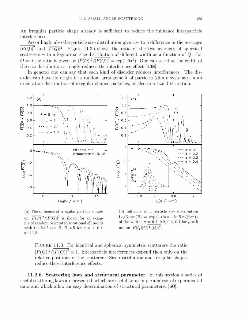
11.2. SMALL ANGLE SCATTERING 455
An irregular particle shape already is sufficient to reduce the influence interparticleinterferences.
Accordingly also the particle size distribution give rise to a difference in the averages
|F (Q)|2 and |F (Q)|2. Figure 11.3b shows the ratio of the two averages of sphericalscatterers with a lognormal size distribution of different width as a function of Q. For
Q = 0 the ratio is given by |F (Q)|2/|F (Q)|2 = exp(−9σ2). One can see that the width ofthe size distribution strongly reduces the interference effect [138].
In general one can say that each kind of disorder reduces interferences. The dis-order can have its origin in a random arrangement of particles (dilute systems), in anorientation distribution of irregular shaped particles, or also in a size ditsribution.
(a) The influence of irregular particle shapes
on |F (Q)|2/|F (Q)|2 is shown for an exam-ple of random orientated rotational ellipsoidswith the half axis R, R, νR for ν = 1, 0.1,and 1.3.
(b) Influence of a particle size distribution
LogNorm(R) = exp(−(lnµ− lnR)2/(2σ2)
)of the widths σ = 0.1, 0.2, 0.3, 0.4 for µ = 5
nm on |F (Q)|2/|F (Q)|2.
Figure 11.3. For identical and spherical symmetric scatterers the ratio
|F (Q)|2/|F (Q)|2 ≡ 1. Interparticle interferences depend then only on therelative positions of the scatterers. Size distribution and irregular shapesreduce these interference effects.
11.2.6. Scattering laws and structural parameter. In this section a series ofuseful scattering laws are presented, which are useful for a simple analysis of experimentaldata and which allow an easy determination of structural parameters. [50].
456 11. SCATTERING THEORY
11.2.6.1. Porod volume. The ratio of the scattering intensity in forward directionI(Q = 0) = N V 2
P ∆η2 and the scattering invariant Q = 2π2∆η2 V fp(1 − fp) can beused to determine the particle volume VP (V describes the illuminated sample volume).fp V = N VP corresponds to the total volume of all scatterers whereby the particlevolume VP can be calculated by
VP1− fp
fp1' VP = 2π2 I(Q = 0)
Q. (11.69)
The measurement of the scattering curve in relative units is therefore sufficiant to deter-mine the volume of a homogeneous scatterer. Sources of errors for this way of determi-nation of particle sizes are the extrapolation into forward direction und more importantthe extrapolation to large scattering angles (Q−4-extrapolation). Furthermore for largevolume fractions fp the particle volume has to be eventually corrected by a prefactor1/(1− fp) which is not always known.
11.2.6.2. Radius of gyration and Guinier approximation. The scattering intensity forsmall angles can be approximated in a series expansion by replacing the expression sinQr
Qr
in eq. 11.40 by a McLaurin series which leads to
I(Q) = V
∫4π r2 γ(r)
[1− Q2r2
3!+Q4r4
5!− . . .
]dr , (11.70)
i.e. I(Q) is expanded by moments rn of γ(r). The first term corresponds to the scatteringintensity of Q = 0. For the second term Guinier and Fournet [50] have shown, that itcan be related to the gyration radius of the scattering length density RG by
V
∫4π r2 Q
2r2
3!γ(r) dr = I(0)
Q2R2G
3⇒ I(Q) = I(0)
(1− Q2R2
G
3
)(11.71)
with R2G =
∫η(r) r2 dr/
∫η(r) dr. Up to the term of Q4 this series expansion at the
beginning of the scattering curve is identical to the series expansion of an exponentialfunction which than leads to the well known Guinier approximation
I(Q) = I(0) e−Q2R2
G/3. (11.72)
The Guinier law is valid for any particle shape which is roughly isodiametric. For flat orelongated structures the Guinier law has to be corrected slightly [38, 50]. The radius
of gyration for a sphere with radius R is given by RG =√
3/5 R. The Guinier law isvalid in the scattering vector interval 0 < Q < 1/RG.
11.2.6.3. Correlation length. Another characteristic quantity, which can be easilyextracted from the scattering curve I(Q) is the correlation length lc. The correlationlength is defined as the average width of the correlation function γ(r):
lc =2
γ(0)
∫γ(r) dr. (11.73)
Together with the definition of the scattering invariant Q in eq. 11.49 and the relationbetween I(Q) and γ(r) in eq. 11.44 this results after a short calculation (changing of
11.2. SMALL ANGLE SCATTERING 457
integrations) to
lc = π
∫QI(Q) dQ∫Q2 I(Q) dQ
. (11.74)
A sphere with radius R has therefore a correlation length of lc = 32R.
11.2.6.4. Porod law and specific surfaces. The Porod law describes the scatteringbehavior at large Q values. As the scattering intensity I(Q) and the correlation functionγ(r) are related via the Fourier transformation the intensity I(Q) is determined at largevalues of Q mainly by γ(r) at small r. For small r the correlation function γ(r) can beexpanded in a Taylor series and one gets according to Guinier and Fournet [50]
γ(r)
γ(0)= 1− 1
4
S
V+ . . . , (11.75)
whereby S is the total surface of all scatterer in the illuminated sample volume V . Eq.11.75 together with 11.40 result for large Q values into the Porod law
I(Q) −→ ∆η2 2π S
Q4. (11.76)
A scaling of the scattering intensity on Q provides an expression for the specific surfaceS/V of
limQ→∞
πI(Q)
QQ4 fp (1− fp) =
S
V. (11.77)
The Porod law can be applied to all systems having sharp interfaces.

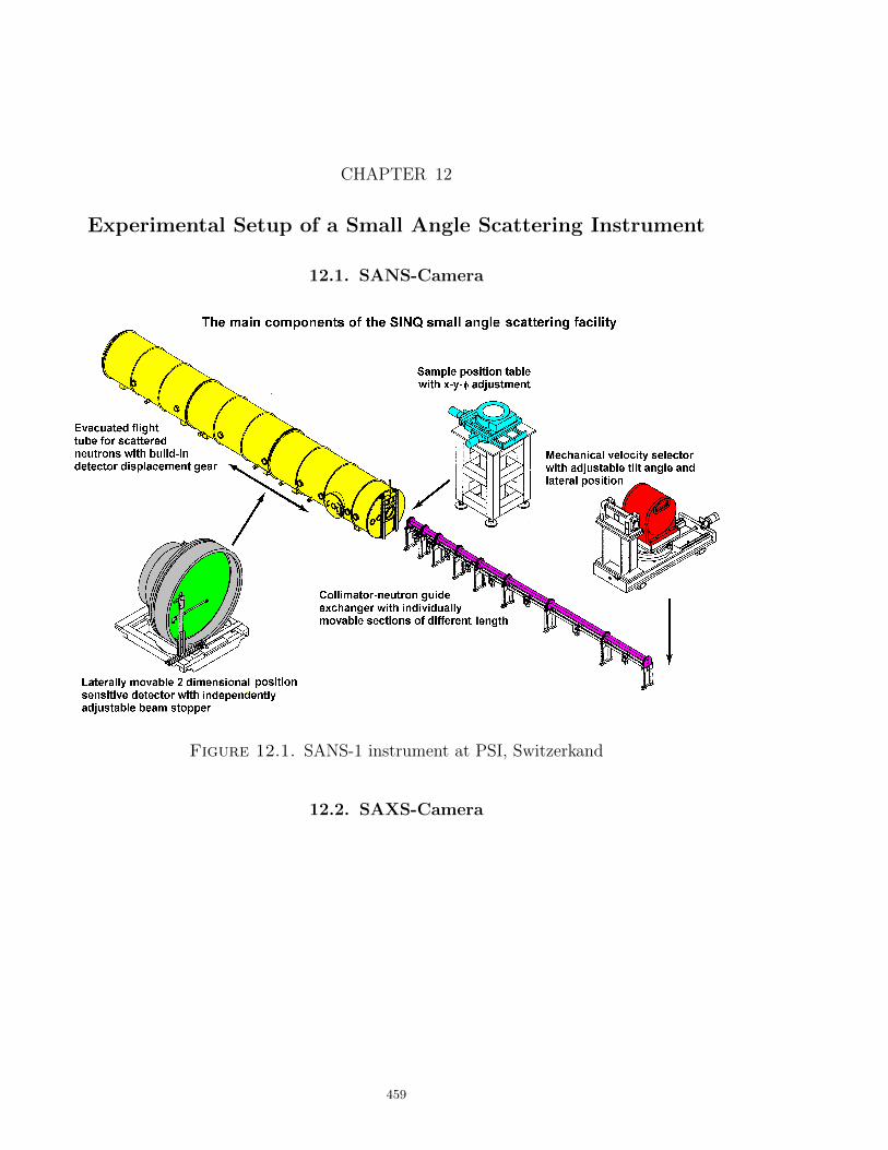
CHAPTER 12
Experimental Setup of a Small Angle Scattering Instrument
12.1. SANS-Camera
Figure 12.1. SANS-1 instrument at PSI, Switzerkand
12.2. SAXS-Camera
459

460 12. EXPERIMENTAL SETUP OF A SMALL ANGLE SCATTERING INSTRUMENT
Figure 12.2. Small angle x-ray scattering instrument Jusifa at the syn-chrotron light source HASYLAB in Hamburg
CHAPTER 13
Data Reduction in SAS
13.1. Correction and Normalization of SANS-Raw data
A detector of a small angle scattering camera measures the superposition of intensitiesof different origin:
(1) Background noise IB(2) Scattering of the empty sample holder IH(3) scattering of the isolated sample IS
Furthermore the detector elements can have different efficiencies εi. To determine the dif-ferential cross-section of of the sample all the different contribution to the total scatteringintensity have to be considered and determined separately by different measurements.The quantity to be known is the scattering contribution of the isolated sample IS, whichin general can not be measured directly. Experimental accessible scattering contribu-tions are the scattering of the sample in the sample holder IS+H , the contribution of theempty sample holder IH and the background noise IB. From this experimental accessibledata the wanted scattering contribution of the isolated sample has to be determined.
13.1.1. Contribution of the isolated sample. The intensity of the incidentbeam will be attenuated by absorption and scattering effects within the sample. Alsothe scattered neutrons will be further attenuated on their residual path through thesample. The measured intensity in a detector element i is given by
I0S,i =
d∫0
dxΦ0 ∆Ωi εi e−αxAρ e−
α(d−x)cos θ
dσcoh
dΩ+dσinc
dΩ
. (13.1)
Hereby d describes the sample thickness in cm, Φ0 the incident neutron flux in neutronsper cm2×sec, dΩi is the solid angle of the detector element i in steradian, εi the detectionefficiency of detector element i and α the extinction coefficient of the sample in cm−1.A the illuminated sample area in cm2. θ describes the angle between the wave vectork0 of the incident neutrons and the wave vector k of the scattered neutrons. dσcoh
dΩand
dσinc
dΩare the coherent and incoherent differential cross-sections, respectively. For small
angle scattering cos θ ' 1 and one yields after integration
I0S,i = Φ0 ∆Ωi εi Aρd︸ ︷︷ ︸
NS
e−αd︸︷︷︸TS
dσcoh
dΩ+dσincdΩ
. (13.2)
The quantity NS = Aρd corresponds to the number of scattering atoms and TS =e−αd = Itrans
I0to the transmissions coefficient, which can be determined from the ration
of the intensity of the transmitted primary beam Itrans and the intensity of the incident
461

462 13. DATA REDUCTION IN SAS
beam I0. The incoherent scattering is isotropically and equally distributed over thewhole solid angle of 4π. Therefore one gets for I0
S,i
I0S,i = Φ0 ∆Ωi εi
NS TS
dσcoh
dΩ+ A
1− TS4 π
. (13.3)
13.1.2. Correction for sample holder and background noise. The scatteringintensity of an isolated sample can practically never measured directly. The scattering ofthe sample is always superposed by scattering from the sample holder and by backgroundnoise. Background noise is meant to be electronic noise, cosmic radiation, and detectionof neutrons, which have not passed through the sample like scattered neutrons fromneighboring experiments. Because of this reasons additional measurements have to becarried out, which are a measurement of the empty sample holder IH and a measurementwith a strong absorber like Cadmium in front of the sample to measure the backgroundnoise IB. Together with the measurement of the sample in the sample holder IS+H,i thescattering of the isolated sample I0
S,i on the detector element i can be calculated by
I0S,i =
(IS+H,i
MS+H
− IB,iMB
)− TS+H
TH
(IH,iMH
− IB,iMB
). (13.4)
The index B stands for background, H for the empty sample holder, S+H for the samplein the sample holder and S for the scattering of the isolated sample. All intensities haveto be normalized on the number of incident neutrons. This can be done for example bydivision of the measured intensity my a monitor count rate M . The factor TS+H
THtakes
account for the attenuation of the beam by the sample.The differential cross-section in eq. 13.3 can now be calculated from the measurable
intensities in eq. 13.4. Nevertheless the quantities Φ0, ∆Ωi and εi still have to be known.Furthermore I0
S is not given in physical standard units but in units per monitor count.All this can be overcome by a comparison with a standard substance St. Commonstandard materials are in general materials with a small coherent cross-section and alarge incoherent cross-section like vanadium or water. For both of these materials thecoherent cross-section is negligible small. The scattering intensities of the standardmaterials have to be corrected in the same way than the sample itself according to eq.13.4. The ratio of both intensities I0
S,i/I0St,i leads to
I0S,i
I0St,i
=
TS NS
(dσcoh
dΩ+dσinc
dΩ
)TStNSt
dσStinc
dΩ
(13.5)
⇔ dσcoh
dΩ+dσinc
dΩ=
I0S,i
I0St,i
TStNSt
TS NS
dσStinc
dΩ(13.6)
ordσcoh
dΩ+dσinc
dΩ=
I0S,i
I0St,i
(1− TSt)ASt4π
TS NS
. (13.7)
If water is used as a standard the last formula has to be multiplied on the right sidewith an empirical factor f(λ, σt, T ) ' 1. This factor corrects for the different efficiencies
13.2. CORRECTION AND NORMALIZATION OF SAXS RAW DATA 463
of the detector for different neutron energies. This correction can become important incase of water because of it inelastic scattering behavior.
13.2. Correction and normalization of SAXS raw data

464 13. DATA REDUCTION IN SAS
History
2014-02-06: SASfit 0.94.2• new binding for zoom option, which works better for a mouse with one
button (plot zoom by ctrl+left-mouse btn)• removed ¡delete¿ key binding for scattering contributions• Added several iteration schemes for finding the fixpoint of the OZ equation.• Added a tab for the total correlation function h(r)• Added also some root finding algorithms for solving OZ equation.• resolution parameter from file was not scaled during the change of units
for Q• bug fix in calculation of xi for sq for wormlike structures (PS1 model)• wrong label for contrast in Teubner-Strey model• bug fix in SPHERE+R-a Nagg form factor in assignement of core volume• data export format set to scientific notation in the form x.yyyE?zz only
2014-02-05: SASfit 0.94.1• added missing parameter label for Hamaker constant in DLVO potential• Penetrable Sphere Model was not properly assigned.• added all available plugins into the distribution binaries
2014-01-20: SASfit 0.94.0• A new interface for solving the Ornstein Zernike equation for different
closure relations and potentials (OZ-solver) has been added. The solutionsof the OZ-solver can be used as a structure factor as a spline functionwithout the possibility to fit a parameter of the potential at the moment.• manual has been extended for the ferrofluid plugin scattering functions• orientation of the 2D simulation was rotated by 90deg.• correction of the manual for Porod’s approximation of cylinders.• minor bug fix for Porod’s approximation of long cylinders.
2013-06-09: SASfit 0.93.5• implementation of a plugin for a form factor and correlation function for
spin misalignment• bug fix for the scattering contribution of the individual chains in the form
factors WORM*, ROD*, and DISC*
• bug fix in the form factor MagneticShellCrossTerm• added some subfolders for form factor plugins• bug fix in the calculation of the scattering length density SLD(E) of x-rays
2013-04-30: SASfit 0.93.4• In the menu for confidence interval the non-diagonal elements of correla-
tion matrix are shown together with the confidence interval for the fittedparameters as diagonal elements.• added some additional parameters into the fit menu useful to evaluate the
goodness of a fit• new plugin for Parallelepiped abc of dimension a*b*c to be found under[by plugins|anisotropic obj]
• new plugin for generalized Guinier law to be found under [by
plugins|non-particular structures]

13.2. CORRECTION AND NORMALIZATION OF SAXS RAW DATA 465
• Renamed HMI format into BerSANS format and did some debugging. Nowalso all masked data points (negative errors) are ignored.• added key bindings Home, End, PgUp, PgDn, Insert, Delete for going to
first-last-next-previous entry or to add and remove an entry• adding plugin with a series of form factor for strongly anisotropic structures
with local planar and local cylindrical shapes• adding a new plugin form factor for spheres with fuzzy interfaces. The
existing form factors ExpShell, LinShell and LinShell2 have been movedto this plugin.• New plugin of FuzzySphere and CoreShellMicrogel. Also the related
functions for calculating the corresponding radial profiles have been added.• new section in the manual about absolute scale, molecular weight, etc.• for the form factors flat cylinder long cylinder, and Porod cylinder
the limiting case q ≡ 0 is now treated properly• small bug fix in the peak function Gamma (Area) for checking validity of
parameter• bug fix of the resolution parameter handling in case it will be read in from
a data file• included under peak function the Maxwell distribution and thegeneralized Maxwell distribution• batch fitting
2011-05-04: SASfit 0.93.3• bug fix in the model Stacked Discs. The structure factor describing the
stacking order contained a bug.• extended plugin for stroboscopic measurements, especially for TISANE• plotting: ignore negative y values on log() and sqrt() scales• included Pcs homogeneousCyl form factor• bug fix of ferrofluid plugin
• added radial averaged form factor in ferrofluid plugin
• extended the spline plugin to be used also as form factors. In case somebodywants to fit a spline function to e.g. a TEM size distribution, this functionneed to be available as a form factor and not only as a size distribution.• added configuration file config.ini as replacement for deprecatedsasfit init public.tcl
• added switch for disabling About popup at start time via config file• added checkbox (ascii options) for ignoring zero(0) intensity at the begin-
ning of data• removed , as data column separator• added substitution of ,⇒ . for data columns (german decimal format to
english format)• added interface function for covariance matrix output• covar matrix visualisation with parameter highlighting• added a chapter about particle number densities, volume fraction and ab-
solute intensities in the manual.
466 13. DATA REDUCTION IN SAS
• LogNorm fp size distribution is now plugin function. The new plugin isnot backwards compatible. The manual explains a bit the difficulties indescribing the size distribution in terms of a volume fraction.• added scrollbars for fit parameter window
2010-07-08: SASfit 0.93.2• bug fix in ferrofluid plugin• added radial averaged form factor. Included radial averaged form factors
also for SAW model• Extended the spline plugin to be used also as form factors. In case some-
body wants to fit a spline function to a size distribution, this function needsto be available as a form factor and not only as a size distribution.• forwarding intermediate linear Guinier approximation results to the plot
window (green curve)• display of linear Guinier approximation results in ISP text output window• residuum window updated with linear Guinier approximation residuum• by default disabled, see checkbox in ISP window• fixed SLDCalculator in source package (missing data files)• added KNOWN BUGS.txt (not complete)• optical (layout) GUI improvements:
– removed thick margin around text boxes for ISP/analyt results– added resizeable file list in ISP window– added resizeable ’merge files’ list when loading data files
• added menu-¿tools-¿toggle console to show the console, it is hidden bydefault now• added OPTIM parameter to src/CMakeLists.txt for optimized binary gen-
eration on the underlying hardware, use: ’cmake -DOPTIM=TRUE’• added configuration file config.ini as (working) replacement for depre-
cated sasfit init public.tcl
• added switch for disabling ’about’ popup at start time via config file• added switch to set the default data directory• added checkbox (ascii options) for ignoring zero(0) intensity at the begin-
ning of data2010-05-13: SASfit 0.93.1
removed obsolete print menu entries and fix of textual output bug2010-05-05: SASfit 0.93.0
• copy&paste-able text output, as well as csv export (semicolon separated)for
– integral structural parameters (ISP) data– parameters of contributions– moments of size distribution
• improved/rewritten file selection GUI for ISP series fitting• new and improved plugins: Kratky Sphere, JuelichCoreShell (rewrit-
ten), Langevin• data is always plotted first, below the calculated lines• error bars are drawn behind data points• fixed wrong plotting of very large error bars

13.2. CORRECTION AND NORMALIZATION OF SAXS RAW DATA 467
• for log-plotting on the y-axis, negative data is ignored (not plotted, wasabs() before)• fix to prevent the user from loading a SASfit project file as data• fix in Form-Factor Background (improved numerical stability)• bug fix for saving parameter files on windows• bug fix in gui when selecting form factor TwoAttachedSpheres• bug fix for ”Singular Matrix” error
2010-01-02: SASfit 0.92.3• implemented three different versions for worm like chains as described
in Macromolecules 1996, 29, 7602-7612. They have been imple-mented as structure factors [anistropic obj|P’(Q):local cylindrical
geometry], so that it can be combined with different cross-sectionform factors of local cylindrical objects [anisotropic obj.|Pcs(Q) for
cylindrical obj.].• new form factor plugin for a sphere with 3 shells• new structure factor for a regular cluster up to maximal 5 particle (tetra-
hedron like)• correction of menue entry order for magnetic shell and superparamagnetic
shell• new plugin for ferrofluid particles with a scheme similar to the one of J.S.
Pedersen for Gaussian Chains attached to a spherical particle• bug fix in mMemberedTwistedRing
• two more default plot: Guinier (rods) and Guinier (sheets)
• bug fix in loglogistic peak• implementation of asymptotic limits for fractals, which require a numerical
integration. The integration often fails for large q-values for which anasymptotic solution is available or has been constructed.• reprogrammed SquareWell1 structure factor for a squared well potential• replaced sasfit qromb function by sasfit integrate function in the form
factor for the torus. The sasfit qromb routine did not work for someunknown reason. This needs to be checked.• new structure factor for a thin square well potential• bug fix in BeaucageExpPowLaw2
• Bug fix for setting plot option Holtzer in multiple data set tab• public initialization file sasfit init public.tcl for setting the default
working directory by the user to any path2009-10-08: SASfit 0.92.2
• data reduction without data loss, after loading a project file the data re-duction can be reversed• info message about a guessed error bar is displayed only once when the
ascii options are changed (not for every file)• added tooltip for complete filenames in merge window• color for selected fit region stays at dark grey after loading an old project
file• removed unused help buttons in file open dialogs• fixed error loop when adding new data to previously loaded project file
468 13. DATA REDUCTION IN SAS
• fix for a homedir being e.g. ’U:at startup on Windows• minor correction in the routine to guess the error bar (normalization) when
only two column are supplied• fix of rare error ”form factor param out of range: -1”
13th of September: SASfit 0.92.1• fix for GUI problem with two plugin form factors (contribution updates). If
there are two plugin model functions with a different number of parameters,you can’t switch/cycle trough the contributions anymore (Next, Previous).• fix for saving a parameter file (file creation was disabled by accident in
previous version)8.7.2009: SASfit 0.91.1: Since the previous version of SASfit (0.90.1, January
2009) there were a lot of changes to primarily improve the quality and portabilityof the code. Here is only a short summary of the larger changes done:• added detailed documentation on setup and installation of SASfit , as well
as plugin development (how to add own model functions)• fixed some bugs in plugin framework• added automatic determination of available plugins at build time• enabled static building for plugins• increasing maximum number of model parameter in GUI• verified build compatibility for MacOS• Extended and improved Scattering Length Density (SLD) Calculator. Now
the scattering length density for x-ray energies between 1keV and 24.9 keVcan be calculated.• a few new form factor have been included: generalized Gaussian
coil, generalized Gaussian coil 1, generalized Gaussian coil 2,ellCylShell1, ellCylShell2
12.01.2009: SASfit 0.90.1 : bug-fix in plugin-GUI5.01.2009: SASfit 0.90: new release including full source code and binaries for
windows and linux. Since the previous version of v (0.87, March 2008) therewere a lot of changes to primarily improve the quality and portability of thecode. Here only a short summary of the ’big’ changes done (as of Dec. 17th,2008):(1) Structured the source code into the modules sasfit common, sasfit sd,
sasfit sq, sasfit ff, sasfit core.(2) Switched to CMake build environment for platform independence. Build
and tested SASfit on Linux and Windows, 32bit as well as 64bit.(3) Replaced intensive string comparisons for model function selection in each
iteration step by more reasonable selection of functions pointers at initial-ization time and direct call of the according function at iteration time.
(4) Fixed a lot of bugs and typos in the GUI (but there are still some)(5) Added flexible plugin system for external model functions. This way, all
model functions can be provided as plugins and though move out of the corealgorithms. Also enables easy customization. In the future the modulessasfit sd, sasfit sq, sasfit ff and sasfit peaks will be converted toexternal plugins.
(6) Added sasfit peaks, a new class of model functions containing peaks.
13.2. CORRECTION AND NORMALIZATION OF SAXS RAW DATA 469
(7) Added capability to ship SASfit as standalone executable, allows runningon system without the need of external libraries (e.g. Tcl, BLT, ...)
4.03.2008: (SASfit version 0.87) The last modification in the menu navigationstill had bugs. Hopefully they are removed in this version.
28.02.2008: (SASfit version 0.86) The menu navigation has been debugged andoptimized. Corrected a bug in calculating the polydispersity index (PDI) inDLS cumulant analysis (PDI=Gamma2/Gamma1 2)
25.01.2008: (SASfit version 0.85) A bug for the form factors ROD+Rˆ-a* has beencorrected. The implementation of the scaling approximation, partial structurefactors and local monodisperse approach has been improved.
9.01.2008: (SASfit version 0.84) Form factor for worm-like micelles(WORM+Chains(RW), WORM+Chains(RW) Rc, WORM+Chains(RW) Nagg) and forcluster aggregates (Mass Fractal (Exp(-x) Cut-Off), Fisher-Burford,
MassFractExp,MassFractGauss, Mass Fractal (Exp(-xˆa) Cut-Off),
DLCAggregation, RLCAggregation, MassFractOverlappingSph have beenimplemented. Furthermore a simple scheme for importing data from theclipboard has been implemented, which e.g. allows to copy/paste data fromspread-sheets directly into SASfit. Corrected a bug for the form factorsROD+Rˆ-a*
4.10.2007: (SPHERE+Chains(RW), SPHERE+Chains(RW) Rc,SPHERE+Chains(RW) NaggSASfit version 0.80) Next to the correctionof some bugs a simulation option for multiple data sets has been implemented.Furthermore an option has been implemented to subtract a theoreticalscattering contribution from the experimental data set, like e.g. a constantbackground signal. The format of the project files have up to now never beentested for compatibility. An attempt has been started to change this for thefuture versions.
20.8.2007: A couple of form factors for spherical, elliptical, cylin-drical and very long rod-like micelles consisting of a homogeneouscore and which are either grafted with Gaussian chains *(RW)*, orgrafted with semi-flexible self-avoiding and interacting chains *(SAW)*
or a corona with a power-law decaying profile r−α *(Rˆ-a)* havebeen implemented: SPHERE+Chains(RW), SPHERE+Chains(RW) Rc,
SPHERE+Chains(RW) Nagg, SPHERE+Chains(SAW), SPHERE+Chains(SAW) Rc,
SPHERE+Chains(SAW) Nagg, SPHERE+Rˆ-a, SPHERE+Rˆ-a Rc,
SPHERE+Rˆ-a Nagg, ELL+Chains(RW), ELL+Chains(RW) Rc,
ELL+Chains(RW) Nagg, CYL+Chains(RW), CYL+Chains(RW) Rc,
CYL+Chains(RW) Nagg, ROD+Chains(RW), ROD+Chains(RW) Rc,
ROD+Chains(RW) nagg, ROD+Rˆ-a, ROD+Rˆ-a Rc, ROD+Rˆ-a nagg
30.6.2007: Rudimental copy algorithm to copy plots or parameters into window-clipboard. Everything is copied in wmf-format and the option only works finefor information in non-scrolled widgets. Copy-option can be activated withright mouse button or double click of left mouse button. A triaxial ellipsoidal(triaxEllShell) shell with semiaxis a, b, c and shell thickness t is available.

470 13. DATA REDUCTION IN SAS
4.6.2007: Implementation of form factors for cylindrical shells with circular cross-section and capped ends (CylShell2) and without capped ends (CylShell1)together with an approximation for very long cylindrical shells (LongCylShell)
27.3.2007: Implementation of form factors for bi-continuous systems(TeubnerStrey and DAB)
23.2.2007: Implementation of the structure factor for a system of charged, spher-oidal objects in a dielectric medium according to the RMSA model of Hayterand Penfold
11.11.2006: Implementation of a semiflexible polymer according to Kholodenko,some form factors with plane geometry, which are intended to be usedwith lamellar structure factors (homogenousXS, TwoInfinitelyThinPlates,LayeredCentroSymmetricXS, BiLayerGauss), a sphere with Gaussian chainsattached SphereWithGaussChains and a slightly different parametrised formfactor named BlockCopolymerMicelle. An additional option for reading ASCIIdata files is now available, which allows to convert values for the scattering vec-tor from nm−1 into A−1 and vice versa.
23.10.2006: Implementation of a polydsiperse star PolydisperseStar and offlexible ring polymers FlexibleRingPolymer and mMemberedTwistedRing.
22.10.2006: Implementation of the form factor of a flexible polymer with Gauss-ian statistics (in different parameterisations Gauss, Gauss2, Gauss3) for a poly-disperse flexible polymer with Gaussian statistics (GaussPoly) and a flexiblering of polymer with Gaussian statistics (FlexiblePolymerRing)
12.10.2006: Under the menu option Calc/DLS... next to a cumulant fit also adouble stretched exponential decay can be selected to fit dynamic light scatter-ing data.
5.10.2006: Implementation of a spherical shell with a diffuse (expontential) scat-tering length density profile inside the shell caused by solvent penetration intothe shell
13.9.2006: Implementation of a form factor for spheres with gaussian chains at-tached.
19.7.2006: First release (current version: 0.71) at the moment only a windowsversion is available. The installation files for tcl/tk and blt are included in thedistribution file.
Bibliography
[1] S. Alexander, P. M. Chaikin, P. Grant, G. J. Morales, P. Pincus, and D. Hone. Charge renor-malization, osmotic pressure, and bulk modulus of colloidal crystals: Theory. The Journal ofChemical Physics, 80(11):5776–5781, 1984.
[2] N. W. Ashcroft and L. Lenker. Structure and resistivity of liquid metals. Physical Review,145(1):83–90, May 1966.
[3] P. Ballone, G. Pastore, G. Galli, and D. Gazzillo. Additive and non-additive hard sphere mixtures.Molecular Physics, 59(2):275–290, 1986.
[4] B. Barboy. On a representation of the equation of state of fluids in terms of the adhesive hard-sphere model. J. Chem. Phys., 61(8):3194–3196, 1974.
[5] R.J. Baxter. Percus-yevick equation for hard spheres with surface adhesion. J. Chem. Phys.,49(6):2770–2774, 1968.
[6] G. Beaucage. Approximations leading to a unified exponential/power-law approach to small-anglescattering. J. Appl. Cryst., 28:717–728, 1995.
[7] G. Beaucage. Small-angle scattering from polymeric mass fractals of arbitrary mass-fractal di-mension. J. Appl. Cryst., 29:134–146, 1996.
[8] H. Benoit. On the effect of branching and polydispersity on the angular distribution of the lightscattered by gaussian coils. J. Polym. Sci., 11:507–510, 1953.
[9] Ingo Berndt, Jan Skov Pedersen, Peter Lindner, and Walter Richtering. Influence of shell thicknessand cross-link density on the structure of temperature-sensitive poly-n-isopropylacrylamidepoly-n-isopropylmethacrylamide coreshell microgels investigated by small-angle neutron scattering. Lang-muir, 22(1):459–468, 2006. PMID: 16378460.
[10] Ingo Berndt, Jan Skov Pedersen, and Walter Richtering. Structure of multiresponsive intelligent?coreshell microgels. Journal of the American Chemical Society, 127(26):9372–9373, 2005. PMID:15984856.
[11] Ingo Berndt, Jan Skov Pedersen, and Walter Richtering. Temperature-sensitive coreshell microgelparticles with dense shell. Angewandte Chemie, 118(11):1769–1773, 2006.
[12] Philip Bevington and D. Keith Robinson. Data Reduction and Error Analysis for the Physical Sci-ences. McGraw-Hill, 3rd edition, 23 July 2002. ISBN-10: 0072472278, ISBN-13: 978-0072472271.
[13] A. E. Blaurock. Evidence of bilayer structure and of membrane interactions from x-ray diffractionanalysis. Biochimica et Biophysica Acta (BBA) - Reviews on Biomembranes, 650(4):167 – 207,1982.
[14] C.F. Bohren and D.R. Huffman. Absorption and Scattering of Light by Small Particles. Wiley,New York, 1983.
[15] J. M. Bomont and J. L. Bretonnet. A self-consistent integral equation: Bridge function and ther-modynamic properties for the lennard-jones fluid. The Journal of Chemical Physics, 119(4):2188–2191, 2003.
[16] Jean-Marc Bomont. Recent Advances in the Field of Integral Equation Theories: Bridge Functionsand Applications to Classical Fluids, chapter Chapter 1, pages 1–84. John Wiley & Sons, Inc.,2008.
[17] Jean-Marc Bomont and Jean-Louis Bretonnet. A consistent integral equation theory for hardspheres. The Journal of Chemical Physics, 121(3):1548–1552, 2004.
[18] M. Born and H. S. Green. A general kinetic theory of liquids I. The molecular distribution func-tions. Proc. Roy. Soc., A188:10–18, 1946.
471
472 BIBLIOGRAPHY
[19] W. Burchard. Statistics of star-shaped molecules. i. stars with polydisperse side chains. Macro-molecules, 7:835–841, 1974.
[20] W. Burchard, E. Michel, and V. Trappe. Conformational properties of multiply twisted ringsystems and daisy-like structures. Macromolecules, 29(18):5934–5939, 1996.
[21] C. Caccamo. Integral equation theory description of phase equilibria in classical fluids. PhysicsReports, 274(12):1 – 105, 1996.
[22] A. Caille. X-ray scattering in smectic a. Comptes Rendus des Seances de l’Academie des Sciences,Serie B: Sciences Physiques, 274:891–893, 1972.
[23] I. Charpentier and N. Jakse. Exact numerical derivatives of the pair-correlation function of simpleliquids using the tangent linear method. The Journal of Chemical Physics, 114(5):2284–2292, 2001.
[24] Junzo Chihara. Integral euqations for fluids with long-range and short-range potentials: Applica-tion to a charged particle system. Progress of Theoretical Physics, 50(2):409–423, 1973.
[25] Niharendu Choudhury and Swapan K. Ghosh. Integral equation theory of lennard-jones fluids: Amodified verlet bridge function approach. The Journal of Chemical Physics, 116(19):8517–8522,2002.
[26] G. Damaschun, H.-V. Porschel, and G. Sommer. Bestimmung der Gestalt geloster Makromolekuleaus Rontgen-Kleinwinkeldiagrammen mit Hilfe von Gleichungssystemen. Acta Cryst., A25:708,1969.
[27] G. Damaschun and H.-V. Purschel. Rontgen-Kleinwinkelstreuung von isotropen Proben ohneFernordnung. I. Allgemeine Theorie. Acta Crystallographica Section A, 27(3):193–197, May 1971.
[28] M. Daoud and J.P. Cotton. Star shaped polymers - a model for the conformation and itsconcentration-dependence. Journal de Physique (Paris), 43:531, 1982.
[29] W. I. F. David. Powder diffraction peak shapes. parameterization of the pseudo-voigt as a voigtfunction. Journal of Applied Crystallography, 19(1):63–64, Feb 1986.
[30] C. G. de Kruif, P. W. Rouw, W. J. Briels, M. H. G. Duits, A. Vrij, and R. P. May. Adhesive hard-sphere colloidal dispersions. a small-angle neutron-scattering study of stickiness and the structurefactor. Langmuir, 5:422–428, 1989.
[31] P. Debye. Uber die Zerstreuung von Rontgenstrahlen an amorphen Korpern. Physik. Z., 28:135–141, 1927.
[32] P. Debye. Mollecular-weight determination by light scattering. Journal of Physical and ColloidChemistry, 51:18–32, 1947.
[33] P. Debye, R. Anderson, and H. Brumberger. Scattering by an inhomogeneous solid. ii. the corre-lation function and its application. Journal of Applied Physics, 28(6):679, 1957.
[34] P. Debye and A.M. Bueche. Scattering by an inhomogeneous solid. Journal of Applied Physics,20:518–525, 1949.
[35] W. D. Dozier, J. S. Huang, and L. J. Fetters. Colloidal nature of star polymer dilute and semidilutesolutions. Macromolecules, 24(10):2810–2814, 1991.
[36] Der-Ming Duh and A. D. J. Haymet. Integral equation theory for uncharged liquids: The lennard-jones fluid and the bridge function. The Journal of Chemical Physics, 103(7):2625–2633, 1995.
[37] J. Dzubiella, A. Jusufi, C. N. Likos, C. von Ferber, H. Lowen, J. Stellbrink, J. Allgaier, D. Richter,A. B. Schofield, P. A. Smith, W. C. K. Poon, and P. N. Pusey. Phase separation in star-polymer˘colloid mixtures. Phys. Rev. E, 64:010401, Jun 2001.
[38] L. A. Feigin and D. I. Svergun. Structure Analysis by Small-Angle X-ray and Neutron Scattering.Plenum Press, 1987.
[39] S. Forster, N. Hermsdorf, C. Bottcher, and P. Lindner. Structure of polyelectrolyte block copoly-mer micelles, macromolecules. Macromolecules, 35:4096–4105, 2002.
[40] S. Forster, N. Hermsdorf, W. Leube, H. Schnablegger, M. Regenbrecht, S. Akari, P. Lindner, andC. Bottcher. Fusion of charged block copolymer micelles into toroid networks. J. Phys. Chem. B,103:6657–6668, 1999.
[41] Peter Fratzl. Statistical model of the habit and arrangement of mineral crystals in the collagen ofbone. Journal of Statistical Physics, 77(1-2):125–143, 1994.
[42] Matteo Frigo and Steven G. Johnson. The fastest Fourier transform in the west. Technical ReportMIT-LCS-TR-728, Massachusetts Institute of Technology, September 1997.

BIBLIOGRAPHY 473
[43] Matteo Frigo and Steven G. Johnson. The design and implementation of FFTW3. Proceedingsof the IEEE, 93(2):216–231, 2005. Special issue on “Program Generation, Optimization, andPlatform Adaptation”.
[44] Thomas Fruhwirth, Gerhard Fritz, Norbert Freiberger, and Otto Glatter. Structure and orderin lamellar phases determined by small-angle scattering. Journal of Applied Crystallography,37(5):703–710, Oct 2004.
[45] H. Furukawa. Dynamics-scaling theory for phase-separating unmixing mixtures: Growth rates ofdroplets and scaling properties of autocorrelation functions. Physica A, 123:497, 1984.
[46] Domenico Gazzillo, Achille Giacometti, Raffaele Guido Della Valle, Elisabetta Venuti, and FlavioCarsughi. A scaling approximation for structure factors in the integral equation theory of poly-disperse nonionic colloidal fluids. The Journal of Chemical Physics, 111(16):7636–7645, 1999.
[47] O. Glatter. Data evaluation in small angle scattering: Calculation of the radial electron densitydistribution by means of indirect Fourier transformation. Acta Physica Austriaca, 47:83–102, 1977.
[48] Georg S. Greschner. Mathematical properties of polydisperse systems, 2. application to lightscattering. Die Makromolekulare Chemie, 170(1):203–229, 1973.
[49] A. Guinier. X-ray Diffraction. San Francisco: Freeman, 1963.[50] A. Guinier and G. Fournet. Small-Angle Scattering of X-Rays. John Wiley & Sons, Inc., 1955.[51] W. C. Hamilton. Significance tests on the crystallographic R factor. Acta Crystallographica,
18(3):502–510, Mar 1965.[52] B. Hammouda. the sans toolbox. . . . /the SANS toolbox.pdf.[53] H. J. M. Hanley, C. D. Muzny, D. L. Ho, and C. J. Glinka. A small-angle neutron scattering study
of a commercial organoclay dispersion. Langmuir, 19(14):5575–5580, 2003.[54] Jean-Pierre Hansen and Ian R. McDonald. Theory of Simple Liquids with Applications to Soft
Matter. Academic Press, fourth edition, 2013.[55] J.P. Hansen and J.B. Hayter. A rescaled msa structure factor for dilute charged colloidal disper-
sions. Molecular Physics, 46:651–656, 1982.[56] J. B. Hayter and J. Penfold. Use of viscous shear alignment to study anisotropic micellar structure
by small-angle neutron scattering. J. Phys. Chem., 88:4589–4593, 1984.[57] J.B. Hayter and J. Penfold. An analytic structure factor for macroion solutions. Molecular Physics,
42:109–118, 1981.[58] Douglas Henderson, Stefan Soko lowski, and Malgorza la Borowko. Computational Methods in Sur-
face And Colloidal Science, chapter Integral Equations in the Theory of Simple Fluids, pages135–166. Marcel Dekker, Inc., 2000.
[59] O. Hittmair. Lehrbuch der Quantentheorie. Verlag Karl Thiemig, 1972.[60] Rex P. Hjelm, Claudio Schteingart, Alan F. Hofmann, and Devinderjit S. Sivia. Form and structure
of self-assembling particles in monoolein-bile salt mixtures. J. Phys. Chem., 99:16395–16406, 1995.[61] Rex P. Hjelm, Claudio D. Schteingart, Alan F. Hofmann, and P. Thiyagarajan. Structure of conju-
gated bile salt-fatty acid-monoglyceride mixed colloids: Studies by small-angle neutron scattering.J. Phys. Chem. B, 104:197–211, 2000.
[62] Rex P. Hjelm, P. Thiyagarajan, and Hayat Alkan-Onyuksel. Organization of phosphatidylcholineand bile salt in rodlike mixed micelles. J. Phys. Chem, 96:8653–8661, 1992.
[63] Herbert H.H Homeier, Sebastian Rast, and Hartmut Krienke. Iterative solution of the ornstein-zernike equation with various closures using vector extrapolation. Computer Physics Communi-cations, 92(23):188 – 202, 1995.
[64] R. Hosemann and S.N. Bagchi. Direct Analysis of Diffraction by Matter. Amsterdam: North-Holland., 1962.
[65] A.J. Hurd and W.L. Flower. In situ growth and structure of fractal silica aggregates in a flame.Journal of Colloid and Interface Science, 122(1):178–192, 1988.
[66] T. Ida, M. Ando, and H. Toraya. Extended pseudo-voigt function for approximating the voigtprofile. Journal of Applied Crystallography, 33(6):1311–1316, Dec 2000.
[67] J. E. Jones. On the determination of molecular fields. ii. from the equation of state of a gas.Proceedings of the Royal Society of London. Series A, 106(738):463–477, 1924.
474 BIBLIOGRAPHY
[68] A Jusufi, J Dzubiella, C N Likos, C von Ferber, and H Lwen. Effective interactions between starpolymers and colloidal particles. Journal of Physics: Condensed Matter, 13(28):6177, 2001.
[69] Takeshi Kawaguchi. Radii of gyration and scattering functions of a torus and its derivatives. J.Appl. Cryst., 34:580–584, 2001.
[70] Hakon Kaya. Scattering from cylinders with globular end-caps. Journal of Applied Crystallography,37(2):223–230, Apr 2004.
[71] Hakon Kaya and Nicolas-Raphael de Souza. Scattering from capped cylinders. Addendum. Journalof Applied Crystallography, 37(3):508–509, Jun 2004.
[72] A. L. Kholodenko. Analytical calculation of the scattering function for polymers of arbitraryflexibility using the dirac propagator. Macromolecules, 26:4179–4183, 1993.
[73] J. Kohlbrecher, A. Wiedenmann, and H. Wollenberger. Magnetic coupling between the differentphases in nanocrystalline fe-si-b studied by small angle neutron scattering. Zeitschrift fr PhysikB Condensed Matter, 104(1):1–4, August 1997.
[74] M. Kotlarchyk and S.-H. Chen. Analysis of small angle neutron scattering spectra from polydis-perse interacting colooids. J. Chem. Phys, 79(5):2461–2489, 1983.
[75] O. Kratky and G. Porod. Diffuse small-angle scattering of x-rays in colloid systems. Journal ofColloid Science, 4(1):35 – 70, 1949.
[76] J. L. Lebowitz and J. K. Percus. Mean spherical model for lattice gases with extended hard coresand continuum fluids. Phys. Rev., 144:251–258, Apr 1966.
[77] Lloyd L. Lee. An accurate integral equation theory for hard spheres: Role of the zero-separationtheorems in the closure relation. The Journal of Chemical Physics, 103(21):9388–9396, 1995.
[78] Henk N.W. Lekkerkerker and Remco Tuinier. Colloids and the Depletion Interaction, volume 833of Lecture Notes in Physics. Springer Netherlands, 2011.
[79] C. N. Likos, H. Lowen, M. Watzlawek, B. Abbas, O. Jucknischke, J. Allgaier, and D. Richter.Star polymers viewed as ultrasoft colloidal particles. Phys. Rev. Lett., 80:4450–4453, May 1998.
[80] Christos N. Likos. Effective interactions in soft condensed matter physics. Physics Reports,348(45):267 – 439, 2001.
[81] Christos N. Likos. Microgel Suspensions: Fundamentals and Applications, chapter Chapter 7.Structure and Thermodynamics of Ionic Microgels, pages 163–193. Wiley-VCH Verlag GmbH &Co. KGaA, 2011.
[82] M.Y. Lin, H.M. Lindsay, D.A. Weitz, R.C. Ball, R. Klein, and P. Meakin. Universality of fractalaggregates as probed by light scattering. Proc. R. Soc. Lond. A, 423:71–87, 1989.
[83] M.Y. Lin, H.M. Lindsay, D.A. Weitz, R.C. Ball, R. Klein, and P. Meakin. Universal diffusion-limited colloid aggregation. J. Phys.: Condens. Matter, 2:3093–3113, 1990.
[84] M.Y. Lin, H.M. Lindsay, D.A. Weitz, R.C. Ball, R. Klein, and P. Meakin. Universal reaction-limited colloidal aggregation. Physical Review A, 41(4):2005–2020, 1990.
[85] Yuyan Liu, Jieli Lin, Guangming Huang, Yuanqing Guo, and Chuanxi Duan. Simple empiricalanalytical approximation to the voigt profile. J. Opt. Soc. Am. B, 18(5):666–672, 2001.
[86] E. Lomba and L.L. Lee. Consistency conditions for the integral equations of liquid structures.International Journal of Thermophysics, 17(3):663–672, 1996.
[87] A. A. Louis, P. G. Bolhuis, and J. P. Hansen. Mean-field fluid behavior of the gaussian core model.Phys. Rev. E, 62:7961–7972, Dec 2000.
[88] Yulia Lyatskaya, Yufeng Liu, Stephanie Tristram-Nagle, John Katsaras, and John F. Nagle.Method for obtaining structure and interactions from oriented lipid bilayers. Phys. Rev. E,63(1):011907, Dec 2000.
[89] William G. Madden and Stuart A. Rice. The mean spherical approximation and effective pairpotentials in liquids. The Journal of Chemical Physics, 72(7):4208–4215, 1980.
[90] C. Marquest and T.A. Witten. Simple cubic structure in copolymer mesophases. J. Phys. France,50(10):1267–1277, 1989.
[91] G. A. Martynov and A. G. Vompe. Differential condition of thermodynamic consistency as aclosure for the ornstein-zernike equation. Phys. Rev. E, 47:1012–1017, Feb 1993.
[92] G.A. Martynov and G.N. Sarkisov. Exact equations and the theory of liquids. v. Molecular Physics,49(6):1495–1504, 1983.
BIBLIOGRAPHY 475
[93] S.V.G. Menon, V.K. Kelkar, and C. Monohar. Application of baxters model to the theory of cloudpoints of nonionic surfactant solutions. Physical Review A, 43(2):1130–1133, 1991.
[94] S.V.G. Menon, C. Manobar, and K. Srinivasa Rao. A new interpretation of a sticky hard spheremodel. J. Chem. Phys., 95(12):9186–9190, 1991.
[95] Andreas Michels and Jens-Peter Bick. Autocorrelation function of the spin misalignment in mag-netic small-angle neutron scattering: application to nanocrystalline metals. Journal of AppliedCrystallography, 46(3):788–790, Jun 2013.
[96] G. Mie. Beitrage zur Optik truber Medien, speziell kolloidaler Metallosungen. Annalen der Physik,25:377–455, 1908.
[97] B.M. Mladek, M.J. Fernaud, G. Kahl, and M. Neumann. On the thermodynamic properties ofthe generalized gaussian core model. Condensed Matter Physics, 8:135–148, 2005.
[98] J. Moller, R. Kranold, J. Schmelzer, and U. Lembke. Small-Angle X-ray Scattering Size Param-eters and Higher Moments of the Particle-Size Distribution Function in the Asymptotic Stage ofOstwald Ripening. Journal of Applied Crystallography, 28(5):553–560, Oct 1995.
[99] R. M. Moon, T. Riste, and W. C. Koehler. Polarization analysis of thermal-neutron scattering.Physical Review, 181(2):920–931, May 1969.
[100] F. Muller, M. Delsanti, L. Auvray, J. Yang, Y.J. Chen, J.W. Mays, B. Dem, M. Tirrell, , andP. Guenoun. Ordering of urchin-like charged copolymer micelles: Electrostatic, packing and poly-electrolyte correlations. Eur. Phys. J. E, 3:45–53, 2000.
[101] Gerhard Ngele. On the dynamics and structure of charge-stabilized suspensions. Physics Reports,272(5-6):215 – 372, 1996.
[102] Gerhard Ngele. The Physics of Colloidal Soft Matter. Number 14 in Lecture Notes. Institute ofFundamental Technological Research - Polish Academy of Sciences, Warsaw, 2004.
[103] Online Dictionary of crystallography. R factor. http://reference.iucr.org/dictionary/R factor.[104] J. J. Olivero and R. L. Longbothum. Empirical fits to the voigt line width: A brief review. J.
Quant. Spectrosc. Radiat. Transfer, 17(233-236):1298, 1977.[105] L.S. Ornstein and F. Zernike. Accidental deviations of density and opalescence at the critical
point of a single substance. Koninklijke Nederlandsche Akademie van Wetenschappen Proceedings,17:793–806, 1914.
[106] S.M. Oversteegen and H.N.W. Lekkerkerker. On the accuracy of the derjaguin approximation fordepletion potentials. Physica A: Statistical Mechanics and its Applications, 341(1-4):23–39, 2004.cited By (since 1996)12.
[107] G. Pabst, R. Koschuch, B. Pozo-Navas, M. Rappolt, K. Lohner, and P. Laggner. Structuralanalysis of weakly ordered membrane stacks. Journal of Applied Crystallography, 36(6):1378–1388,Dec 2003.
[108] Georg Pabst, Michael Rappolt, Heinz Amenitsch, and Peter Laggner. Structural information frommultilamellar liposomes at full hydration: Full q -range fitting with high quality x-ray data. Phys.Rev. E, 62:4000–4009, Sep 2000.
[109] J. S. Pedersen, D. Posselt, and K. Mortensen. Analytical treatment of the resolution function forsmall-angle scattering. Journal of Applied Crystallography, 23(4):321–333, Aug 1990.
[110] J. S. Pedersen and P. Schurtenberger. Scattering functions of semiflexible polymers with andwithout excluded volume effects. Macromolecules, 29:7602–7612, 1996.
[111] Jan Skov Pedersen. Neutrons, X-Rays and Light, chapter Modelling of Small-Angle ScatteringData from Colloids and Polymer Systems, pages 391–420. Elsevier Science, 2002.
[112] Jan Skov Pedersen and Michael C. Gerstenberg. Scattering form factor of block copolymer mi-celles. Macromolecules, 29(4):1363–1365, 1996.
[113] J.S. Pedersen. Form factors of block copolymer micelles with spherical, ellipsoidal and cylindricalcores. Journal of Applied Crystallography, 33(3 Part 1):637–640, Jun 2000.
[114] .S. Pedersen. Determination of size distributions from small-angle scattering data for systems witheffective hard-sphere interactions. J. Appl. Cryst., 27:595–608, 1994.
[115] J. K. Percus and G. J. Yevick. Analysis of classical statistical mechanics by means of collectivecoordinates. Phys. Rev., 110(1):1–13, 1958.
476 BIBLIOGRAPHY
[116] Horia I. Petrache, Nikolai Gouliaev, Stephanie Tristram-Nagle, Ruitian Zhang, Robert M. Suter,and John F. Nagle. Interbilayer interactions from high-resolution x-ray scattering. Phys. Rev. E,57(6):7014–7024, Jun 1998.
[117] G. Porod. Die Abhangigkeit der Rontgenkleinwinkelstreuung von Form und Grosse der KolloidenTeilchen in verdunnten Systemen, IV. Acta Physica Austriaca, 2:255–292, 1948.
[118] William H. Press, Saul A. Teukolsky, William T. Vetterling, and Brian P. Flannery. NumericalRecipes. The Art of Scientific Computing. Cambridge University Press, 3rd edition, 2007.
[119] C. V. Raman. Lxi. on the mean distance between neighbouring molecules in a fluid. Phil. Mag.,47:671–679, 1924.
[120] C. Regnaut and J. C. Ravey. Application of the adhesive sphere model to the structure of colloidalsuspensions. The Journal of Chemical Physics, 91(2):1211–1221, 1989.
[121] C. Regnaut and J. C. Ravey. Erratum: Application of the adhesive sphere model to the struc-ture of colloidal suspensions [j. chem. phys. 91, 1211 (1989)]. The Journal of Chemical Physics,92(5):3250–3250, 1990.
[122] C. Robertus, W.H. Philipse, J.G.H. Joosten, and Y.K. Levine. Solution of the percus-yevickapproximation of the multicomponent adhesive sphere system to the small angle x-ray scatteringfrom microemulsions. J. Chem. Phys., 90(8):4482–4490, 1989.
[123] Forrest J. Rogers and David A. Young. New, thermodynamically consistent, integral equation forsimple fluids. Phys. Rev. A, 30:999–1007, Aug 1984.
[124] D. Roux and C.R. Safinya. A synchrotron x-ray study of competing undulation and electrostaticinterlayer interactions in fluid multimembrane lyotropic phases. J. Phys. France, 49(2):307–318,1988.
[125] K.-V. Schubert, R. Strey, S. R. Kline, and E. W. Kaler. Small angle neutron scattering nearlifshitz lines: Transition from weakly structured mixtures to microemulsions. J. Chem. Phys.,101:5343, 1994.
[126] S. Schwartz, J.E. Cain, E.A. Dratz, and J.K. Blasie. An analysis of lamellar x-ray diffraction fromdisordered membrane multilayers with application to data from retinal rod. Biophysical Journal,15:1201 – 1233, 1975.
[127] R. V. Sharma and K. C. Sharma. The structure factor and the transport properties of dense fluidshaving molecules with square well potential, a possible generalization. Physica A: Statistical andTheoretical Physics, 89(1):213 – 218, 1977.
[128] B. Sjoberg. Small-angle X-ray investigation of the equilibria between copper(II) and glycyl-l-histidylglycine in water solution. A method for analysing polydispersed systems. Journal of Ap-plied Crystallography, 7(2):192–199, Apr 1974.
[129] William R. Smith, Douglas Henderson, and Yoshio Tago. Mean spherical approximation andoptimized cluster theory for the squar-well fluid. The Journal of Chemical Physics, 67(11):5308–5316, 1977.
[130] C. M. Sørensen, J. Cai, and N. Lu. Test of static structure factors for describing light scatteringfrom fractal soot aggregates. Langmuir, 8:2064–2069, 1992.
[131] C. M. Sørensen and G. M. Wang. Size distribution effect on the power law regime of the structurefactor of fractal aggregates. Physical Review E, 60(6):7143–7148, 1999.
[132] G. L. Squires. Thermal Neutron Scattering. Cambridge University Press, 1978.[133] Markus Stieger, Jan Skov Pedersen, Peter Lindner, and Walter Richtering. Are thermorespon-
sive microgels model systems for concentrated colloidal suspensions? a rheology and small-angleneutron scattering study. Langmuir, 20(17):7283–7292, 2004. PMID: 15301516.
[134] Carsten Svaneborg and Jan Skov Pedersen. Form factors of block copolymer micelles withexcluded-volume interactions of the corona chains determined by monte carlo simulations. Macro-molecules, 35(3):1028–1037, 2002.
[135] M. Teubner and R. Strey. Origin of the scattering peak in microemulsions. J. Chem. Phys.,87:3195, 1987.
[136] O. Toon and T. Ackerman. Algorithms for the calculation of scattering by stratified spheres.Applied Optics, 20(20):3657, 1981.

BIBLIOGRAPHY 477
[137] Johan Ulander, Hans Greberg, and Roland Kjellander. Primary and secondary effective chargesfor electrical double layer systems with asymmetric electrolytes. The Journal of Chemical Physics,115(15):7144–7160, 2001.
[138] P. van Beurten and A. Vrij. Polydispersity effects in the small-angle scattering of concentratedsolutions of colloidal spheres. J. Chem. Phys., 74(5):2744–2748, March 1981.
[139] H.C. van de Hulst. Light Scattering by Small Particles. Wiley, New York, 1957.[140] Loup Verlet. Integral equations for classical fluids. Molecular Physics, 41(1):183–190, 1980.[141] Loup Verlet. Integral equations for classical fluids. Molecular Physics, 42(6):1291–1302, 1981.[142] Linda Viererblova, Jiri Kolafa, Stanislav Labik, and Anatol Malijevsky. Virial coefficients and
equation of state of the penetrable sphere model. Phys. Chem. Chem. Phys., 12:254–262, 2010.[143] A. G. Vompe and G. A. Martynov. The bridge function expansion and the self-consistency problem
of the ornstein-zernike equation solution. The Journal of Chemical Physics, 100(7):5249–5258,1994.
[144] C. G. Vonk. On two methods for determination of particle size distribution functions by meansof small-angle x-ray scattering. J. Appl. Cryst., 9:433–440, 1976.
[145] A. Vrij. Mixtures of hard spheres in the percus-yevick approximation. light scattering at finiteangles. J. Chem. Phys., 71(8):3267–3270, 1979.
[146] W. Wagner and J. Kohlbrecher. Modern Techniques For Characterising Magnetic Materials:,chapter Small-angle neutron scattering, pages 65–104. Kluwer Academic Publishers, 2005.
[147] G. Walter, R. Kranold, T. Gerber, J. Baldrian, and M. Steinhart. Particle size distribution fromsmall-angle X-ray scattering data. Journal of Applied Crystallography, 18(4):205–213, Aug 1985.
[148] John D. Weeks, David Chandler, and Hans C. Andersen. Role of repulsive forces in determiningthe equilibrium structure of simple liquids. The Journal of Chemical Physics, 54(12):5237–5247,1971.
[149] M. S. Wertheim. Exact solution of the percus-yevick integral equation for hard spheres. Phys.Rev. Lett., 10:321–323, Apr 1963.
[150] A. Wiedenmann, R. Gahler, C. D. Dewhurst, U. Keiderling, S. Prevost, and J. Kohlbrecher.Relaxation mechanisms in magnetic colloids studied by stroboscopic spin-polarized small-angleneutron scattering. Phys. Rev. B, 84:214303, Dec 2011.
[151] C. M. Wijmans and E. B. Zhulina. Polymer brushes at curved surfaces. Macromolecules, 26:1214–7224, 1993.
[152] L. Willner, A. Poppe, J. Allgaier, M. Monkenbusch, P. Lindner, and D. Richter. Micellization ofamphiphilic diblock copolymers: Corona shape and mean-field to scaling crossover. EPL (Euro-physics Letters), 51(6):628, 2000.
[153] W. Wiscombe. Mie scattering calculations–advances in technique and fast, vector-speed computercodes, ncar tech note tn-140+str. Technical report, National Center For Atmospheric Research,Boulder, Colorado, 1979.
[154] W. Wiscombe. Improved mie scattering algorithms. Appl. Opt., 19:1505–1509, 1980.[155] Takenao Yoshizaki and Hiromi Yamakawa. Scattering functions of wormlike and helical wormlike
chains. Macromolecules, 13(6):1518–1525, 1980.[156] Gilles Zerah and Jean-Pierre Hansen. Self-consistent integral equations for fluid pair distribution
functions: Another attempt. The Journal of Chemical Physics, 84(4):2336–2343, 1986.[157] F. Zernike and J. A. Prins. Die Beugung von Rontgenstrahlen in Flussigkeiten als Effekt der
Molekulanordnung. Zeitschrift fur Physik, XLI:184–194, 1927.[158] Ruitian Zhang, Robert M. Suter, and John F. Nagle. Theory of the structure factor of lipid
bilayers. Phys. Rev. E, 50(6):5047–5060, Dec 1994.[159] Bruno H. Zimm. The scattering of light and the radial distribution function of high polymer
solutions. The Journal of Chemical Physics, 16(12):1093–1099, 1948.


