Many_Body_Lecture_3.pdf

7/28/2019 Many_Body_Lecture_3.pdf

http://slidepdf.com/reader/full/manybodylecture3pdf 1/35

Many-body Green’s Functions

• Propagating electron or hole interacts with other e-

/h+

• Interactions modify (renormalize) electron or hole energies

• Interactions produce finite lifetimes for electrons/holes (quasi-particles)

• Spectral function consists of quasi-particle peaks plus ‘background’

• Quasi-particles well defined close to Fermi energy

• MBGF defined by

{ }

o

oHHo )t','(ψt),(ψ)t','t,,G(

Ψ

ΨΨ= +

state,groundHeisenbergexact

overaveragedoperatorfieldoffunctionncorrelatioi.e.

rrrr T i




• Space-time interpretation of Green’s function• (x,y) are space-time coordinates for the endpoints of the Green’s function• Green’s function drawn as a solid, directed line from y to x

• Non-interacting Green’s function Go represented by a single line

• Interacting Green’s Function G represented by a double or thick single line

time

Add particle Remove particle

t > t’t’

time

Remove particle Add particle

t’ > tt

x

y

y

)t'(t)t',(ψt),(ψ oHHo −ΨΨ + θ yx

t)(t't),(ψ)t',(ψ oHHo −ΨΨ+

θ xy

x

Go(x,y)

x,ty,t’

G(x,y)x,ty,t’




• Lehmann Representation (F 72 M 372) physical significance of G

{ }

oo

onn

n

oSnnSo

-o-n

oSnnSo

oHnnHooHHo

oHHooHHo

nn

n

o

oHHo

tiEtHitiE-tHi-

)t'tEi(E-

t'Hi-t'HitHi-tHi

ee ee

)'(ψ)(ψ)(

e

)e'(ψe)e(ψe

)t','(ψt),(ψ)t','(ψt),(ψ

t)(t't),(ψ)t','(ψ-)t'(t)t','(ψt),(ψ)t','t,,G(

)t','(ψt),(ψ)t','t,,G(

Ψ=ΨΨ=Ψ

ΨΨΨΨ=

ΨΨΨΨ=

ΨΨΨΨ=ΨΨ

−ΨΨ−ΨΨ=

=ΨΨ

Ψ

Ψ

ΨΨ=

++

++

+

+

++

++

+

rr

rr

rrrr

rrrrrr

1

rrrr

θ θ i

T i

formalismnumberoccupationinoperatorunit

numberparticleany,state,Heisenbergexact

state,groundHeisenbergexact




• Lehmann Representation (physical significance of G)

{ }

onebyinnumberparticlereduces ooS

oSoSSS

on

oSnnSo

on

oSnnSo

-o-noSnnSo

-o-noSnnSo

oHHo

ψ

ψ)1N(ψn )(ψ)(ψdn

δ)EE(εψψ

δ)EE(εψψ

e)t','t,,)G(t'-d(t),',G(

t)(t')(e)(ψ)'(ψ

-)t'(t)(

e)'(ψ)(ψ)t','t,,G(

)t','(ψt),(ψ)t','t,,G(

)t'(t

)t'tEi(E

)t'tEi(E-

ΨΨ

Ψ−=Ψ=

−−+ΨΨΨΨ+

+−−ΨΨΨΨ=

=

−ΨΨΨΨ−

−ΨΨΨΨ=

ΨΨ=

+

++

∞+

∞−

+

+

+

∫

∫ −+

+

rrr

rrrr

rr

rrrr

rrrr

ii

ii

i

T i

iε ε

θ

θ




• Lehmann Representation (physical significance of G)

µ

µ

+−−−=−−

−−+−−−=−−

−ΨΨ=ΨΨΨΨ

++−+=−+

−+++−+=−+

+ΨΨ=ΨΨΨΨ

+

++

)1N(E)1N(E)N(E)1N(E

)N(E)1N(E)1N(E)1N(E)N(E)1N(E

ψψψ

)1N(E)1N(E)N(E)1N(E

)N(E)1N(E)1N(E)1N(E)N(E)1N(E

ψψψ

onon

ooonon

2

nSooSnnSo

onon

ooonon

2

oSnoSnnSo

statesparticle1NandNconnects

statesparticle1NandNconnects




• Lehmann Representation (physical significance of G)• Poles occur at exact N+1 and N-1 particle energies

• Ionisation potentials and electron affinities of the N particle system

• Plus excitation energies of N+1 and N-1 particle systems

• Connection to single-particle Green’s function

FbelowstatesforasstatesunoccupiedtolimitedSum

unoccupied

stategroundg)interactin-(nonparticle-singletheis

ε

δ θ

θ

θ

ε

00c

n0cc0 )t'(t)e'(ψ)(ψ

)t'(t0)(t'c(t)c0)'(ψ)(ψ

)t'(t0)t','(ψt),(ψ0)t','t,,(G

0

n

mnnmn*

n

unocc

n

n

nm

*

n

nm,

m

HHo

)t'-(t-

=

∈=−=

−=

−=

+

+

+

++

∑

∑i

i

rr

rr

rrrr




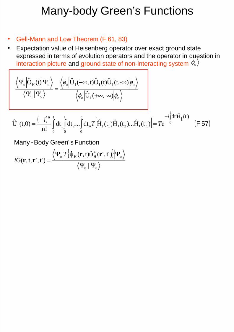
• Gell-Mann and Low Theorem (F 61, 83)• Expectation value of Heisenberg operator over exact ground state

expressed in terms of evolution operators and the operator in question in

interaction picture and ground state of non-interacting system

oIo

oIIIo

oo

oHo

)-,(U

)(t,-U(t)Ot),(U(t)O

φ φ

φ φ

∞+∞

∞+∞=

ΨΨΨΨ

oφ

{ }

oo

oHHo

|

)t','(ψt),(ψ

)t','t,,G( ΨΨ

ΨΨ

=

+ rr

rr

T

i

FunctionsGreen'Body-Many

( ) [ ] ( )57F

)(t'

I

Hdt't

0

t

0

t

0

nI2I1I

t

0

n21

n

I e)(tH)...(tH)(tHdt...dtdtn!

(t,0)U∫ −

=−= ∫ ∫ ∫ i

T T i




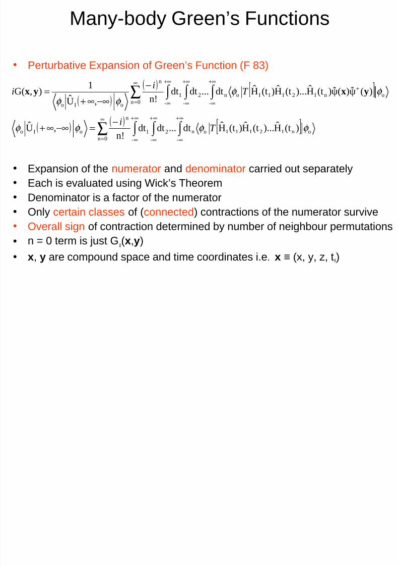
• Perturbative Expansion of Green’s Function (F 83)

• Expansion of the numerator and denominator carried out separately

• Each is evaluated using Wick’s Theorem

• Denominator is a factor of the numerator

• Only certain classes of (connected) contractions of the numerator survive

• Overall sign of contraction determined by number of neighbour permutations

• n = 0 term is just Go(x,y)

• x, y are compound space and time coordinates i.e. x ≡ (x, y, z, tx)

( )

( ) [ ]

( )( ) [ ] o

- -

nI2I1I

-

on21

0n

n

oIo

o

- -

nI2I1I

-

on21

0n

n

oIo

)(tH)...(tH)(tHdt...dtdt

n!

,U

)(ψ)(ψ)(tH)...(tH)(tHdt...dtdtn!,U

1),G(

φ φ φ φ

φ φ φ φ

∫ ∫ ∫ ∑

∫ ∫ ∫ ∑

∞+

∞

∞+

∞

∞+

∞

∞

=

+∞

∞

+∞

∞

++∞

∞

∞

=

−=−∞∞+

−

−∞∞+=

T i

T i

i yxyx




• Fetter and Walecka notation for field operators (F 88)

( )

( )

( )

( ) +−

−+−

+++++

+++++

++

≤=

>=

≤=

+>=

+≡+=

+≡+=

bb- tt ),(G

tt 0)(ψ)(ψ

tt 0

aa tt ),(G)(ψ)(ψ

ba)(ψ)(ψ)(ψ

ba)(ψ)(ψ)(ψ

yxo

yx

)()(

yx

yxo

)()(

(-))(

(-))(

yx

yx

yxyx

xxx

xxx

i

i

( )( )

( ) ( )

0ψψ 0ψψ 0bbabbaaa

bbabbaaa

ba ba

ψψψψψψ (-))()()(

======

+++=

++≡

++=

++++++

++++

++

+++−+++++

similarly




•Nonzero contractions in numerator of MBGF

(-1)3 (i)3v(r,r’)Go(r’,r) Go(r,r’) Go(x,y)

(-1)4(i)3v(r,r’)Go(r,r) Go(r’,r’) Go(x,y)

(-1)5(i)3v(r,r’)Go(x,r) Go(r’,r’) Go(r,y)

(-1)4(i)3v(r,r’)Go(r’,r) Go(x,r’) Go(r,y)

(-1)6(i)3v(r,r’)Go(x,r) Go(r,r’) Go(r’,y)

(-1)7

(i)

3

v(r,r’)Go(r,r) Go(x,r’) Go(r’,y)(6) )(ψ)(ψ)(ψ)'(ψ)'(ψ)(ψ

(5) )(ψ)(ψ)(ψ)'(ψ)'(ψ)(ψ

(4) )(ψ)(ψ)(ψ)'(ψ)'(ψ)(ψ

(3) )(ψ)(ψ)(ψ)'(ψ)'(ψ)(ψ

(2) )(ψ)(ψ)(ψ)'(ψ)'(ψ)(ψ

(1) )(ψ)(ψ)(ψ)'(ψ)'(ψ)(ψ

yxrrrr

yxrrrr

yxrrrr

yxrrrr

yxrrrr

yxrrrr

+++

+++

+++

+++

+++

+++




• Nonzero contractions

-(i)3v(r,r’)Go(r’,r) Go(r,r’) Go(x,y) (1)

+(i)3v(r,r’)Go(r,r) Go(r’,r’) Go(x,y) (2)

-(i)3v(r,r’)Go(x,r) Go(r’,r’) Go(r,y) (3)

+(i)3v(r,r’)Go(r’,r) Go(x,r’) Go(r,y) (4)

+(i)3v(r,r’)Go(x,r) Go(r,r’) Go(r’,y) (5)

-(i)3v(r,r’)Go

(r,r) Go

(x,r’) Go

(r’,y) (6)

y

x

r r’

y

x

r r’

x

y

r r’

y

r r’

x

y

r’ r

xx

y

r’ r

(1) (2)

(3) (4)

(5) (6)



• Nonzero contractions in denominator of MBGF• Disconnected diagrams are common factor in numerator and denominator


(8) )(ψ)'(ψ)'(ψ)(ψ

(7) )(ψ)'(ψ)'(ψ)(ψ

rrrr

rrrr

++

++(-1)3(i)2v(r,r’)Go(r’,r) Go(r,r’)

(-1)4(i)2v(r,r’)Go(r,r) Go(r’,r’)

r r’(7)

r r’

(8)

Denominator = 1 + + + …

Numerator = [ 1 + + + … ] x [ + + + … ]



•Expansion in connected diagrams

• Some diagrams differ in interchange of dummy variables

• These appear m! ways so m! term cancels• Terms with simple closed loop contain time ordered product with equal times• These arise from contraction of Hamiltonian where adjoint operator is on left• Terms interpreted as


∑ ∫ ∫ ∞

=

∞

∞−

∞

∞−

+−=

0m connected

om111om1 ])(ψ)(ψ)(tH ...)(tH[dt...dtm!

)(),G( φ φ yxyx T

ii

iG(x, y) = + + + …

{ }

densitychargeginteractin-non )(ρ)(ψ)(ψ

)t',(ψt),(ψ),(G

ooo

oo

lim

'o

xxx

xxxx

−=−=

=

+

++→

φ φ

φ φ δ T it t



• Rules for generating Feynman diagrams in real space and time (F 97)

• (a) Draw all topologically distinct connected diagrams with m interaction

lines and 2m+1 directed Green’s functions. Fermion lines run continuously

from y to x or close on themselves (Fermion loops)

• (b) Label each vertex with a space-time point x = (r,t)

• (c) Each line represents a Green’s function, Go(x,y), running from y to x

• (d) Each wavy line represents an unretarded Coulomb interaction

• (e) Integrate internal variables over all space and time

• (f) Overall sign determined as (-1)F

where F is the number of Fermion loops• (g) Assign a factor (i)m to each mth order term

• (h) Green’s functions with equal time arguments should be interpreted as

G(r,r’,t,t+) where t+ is infinitesimally ahead of t

• Exercise: Find the 10 second order diagrams using these rules




• Feynman diagrams in reciprocal space

• For periodic systems it is convenient to work in momentum space

• Choose a translationally invariant system (homogeneous electron gas)

• Green’s function depends on x-y, not x,y

• G(x,y) and the Coulomb potential, V, are written as Fourier transforms

• 4-momentum is conserved at vertices


( )

t-.. ddd

)e',v()'-d()v(

)eG(

2

d),G(

34

4

4

)'.(

).(

ω ω

π

xkxkkk

rrrrq

kk

yx

rrq

yxk

≡≡

=

=

∫

∫ −

−

i-

i

Fourier Transforms

( ) ( )321

43214 2eeed...

qqqxxqxqxq −−=

+∫ δ π

-i-ii

4-momentum Conservation

q1

q2

q3



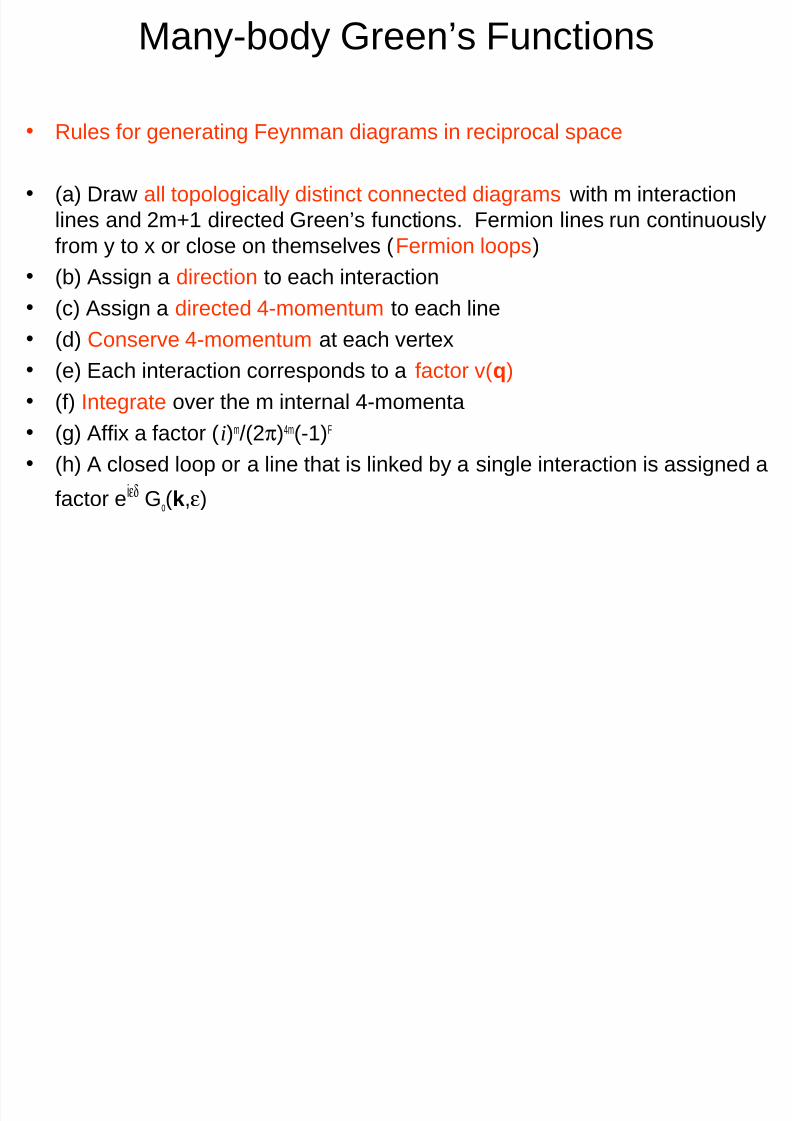
• Rules for generating Feynman diagrams in reciprocal space

• (a) Draw all topologically distinct connected diagrams with m interaction

lines and 2m+1 directed Green’s functions. Fermion lines run continuously

from y to x or close on themselves (Fermion loops)

• (b) Assign a direction to each interaction• (c) Assign a directed 4-momentum to each line

• (d) Conserve 4-momentum at each vertex

• (e) Each interaction corresponds to a factor v(q)

• (f) Integrate over the m internal 4-momenta• (g) Affix a factor (i)m/(2π)4m(-1)F

• (h) A closed loop or a line that is linked by a single interaction is assigned a

factor eiεδ Go(k,ε)




[ ]

[ ]

)(ψ)(ψ1

)(ψ)(ψddH

)(ψ)(ψ1)(ψdH,ψψt

)(ψ)(h)(ψdH

)(ψ)(h H,ψψt

1H2H

21

2H1H21H

H2H

2

2H2HHH

1H11H1H

HHHH

2

1rr

rrrrrr

rrrr

rr

rrrr

rr

−=

−==∂∂

=

==∂∂

++

+

+

∫ ∫

∫

∫

for

for

i

i

Equation of Motion for the Green’s Function

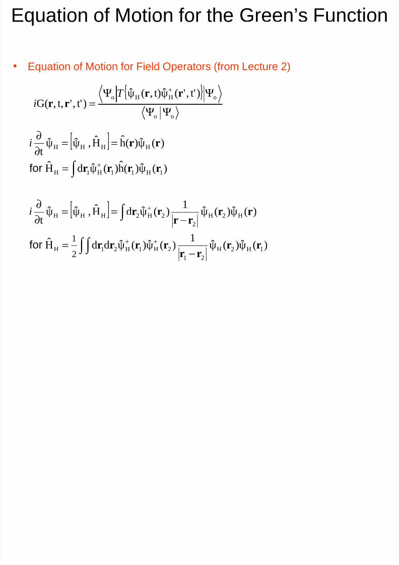
• Equation of Motion for Field Operators (from Lecture 2)

{ }

oo

oHHo )t','(ψt),(ψ)t','t,,G(

ΨΨ

ΨΨ=

+ rrrr

T

i




• Equation of Motion for Field Operators

[ ] [ ]

t),(ψˆ

t),(ψˆ

1

t),(ψˆ

dt),(ψˆ

t),(h

ˆ

t

t),(ψt),(ψ1

t),(ψdt),(ψt),(h

tH

e)(ψ)(ψ

1

)(ψd

tH

e

tH

e)(ψ)(hˆ

tH

e

tHeH,ψtHet),(Ht),,(ψt),(ψt

H2H2

2H2H

H2H

2

2H2H

22

22

SSHHH

rrrrrrrr

rrrr

rrrr

rrrrrrrr

rrr

−=

−∂

∂

−+=

−−

++

−+=

−+==∂∂

+

+

+

∫

∫ ∫

i

iiii

iii




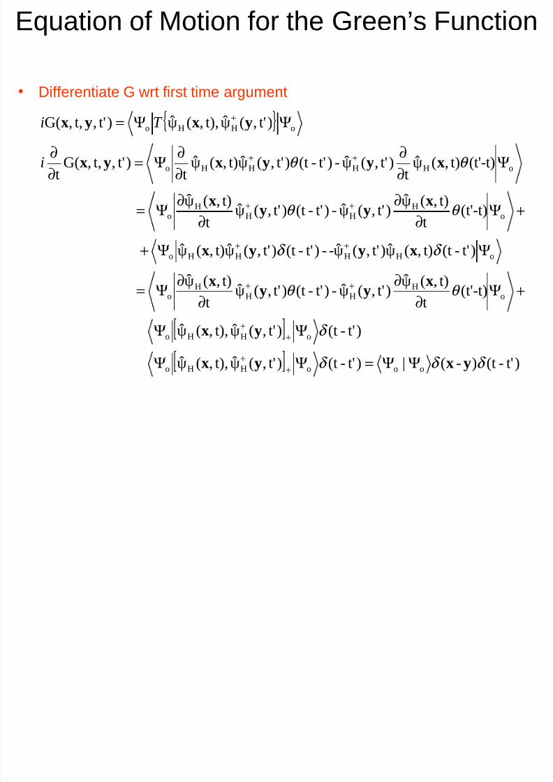
• Differentiate G wrt first time argument

{ }

[ ]

[ ] )t'-(t)-(|)t'-(t)t',(ψt),,(ψ

)t'-(t)t',(ψt),,(ψ

(t'-t)t

t),(ψ)t',(ψ-)t'-(t)t',(ψt

t),(ψ

)t'-(tt),(ψ)t',(ψ--)t'-(t)t',(ψt),(ψ

(t'-t)t

t),(ψ)t',(ψ-)t'-(t)t',(ψ

t

t),(ψ

(t'-t)t),(ψt

)t',(ψ-)t'-(t)t',(ψt),(ψt

)t',t,,G(t

)t',(ψt),,(ψ)t',t,,G(

oooHHo

oHHo

oH

HHH

o

oHHHHo

oH

HHH

o

oHHHHo

oHHo

δ δ δ

δ

θ θ

δ δ

θ θ

θ θ

yxyx

yx

xyyx

xyyx

xyy

x

xyyxyx

yxyx

ΨΨ=ΨΨ

ΨΨ

+Ψ∂∂∂∂Ψ=

ΨΨ+

+Ψ∂

∂∂

∂Ψ=

Ψ∂∂

∂∂

Ψ=∂∂

ΨΨ=

++

++

++

++

++

++

+

i

T i




• Differentiate G wrt first time argument

[ ]

[ ]

)t'-(t)-(

)t',(ψt),(ψt),(ψt),(ψ1

d)t',t,,G(ht

)t'-(t)-(

)t',(ψt),(ψt),(ψt),(ψ

1

d),G(hˆ

)t'-(t)-(

(t'-t)t),(ψt),(ψt),(ψ)t',(ψ-1

d

)t'-(t)t',(ψt),(ψt),(ψt),(ψ1

d

(t'-t)t),(ψ)t',(ψ-)t'-(t)t',(ψt),(ψh)t',t,,G(t

oHH1H1Ho

1

1

oHH1H1Ho1

1

oH1H1HHo

1

1

oHH1H1Ho

1

1

oHHHHo

δ δ

δ δ

δ δ

θ

θ

θ θ

yx

yxrrrx

ryx

yx

yxrrrrryx

yx

xrryrx

r

yxrrrx

r

xyyxyx

=

ΨΨ−

+

−

∂∂

+ΨΨ−−−=

+

ΨΨ−

−

+ΨΨ−

−

+ΨΨ−=∂∂

++

++

++

++

++

∫

∫

∫

∫

T ii

T iii

i

i

ii




• Evaluate the T product using Wick’s Theorem

• Lowest order terms

• Diagram (9) is the Hartree-Fock exchange potential x G o(r1,y)

• Diagram (10) is the Hartree potential x G o(x,y)

• Diagram (9) is conventionally the first term in the self-energy

• Diagram (10) is included in Ho in condensed matter physics

[ ]connectedoHH1H1Ho

1

1 )t',(ψt),(ψt),(ψt),(ψ1

d ΨΨ−

++∫ yxrrrx

r T

)t',(ψt),(ψt),(ψt),(ψ HH1H1H yxrr ++

)t',(ψt),(ψt),(ψt),(ψ HH1H1H yxrr ++

(i)2v(x,r1)Go(x,r1) Go(r1,y)

(i)2v(x,r1)Go(r1,r1) Go(x,y)

x

y

r1

(10)

(9)y

r1

x




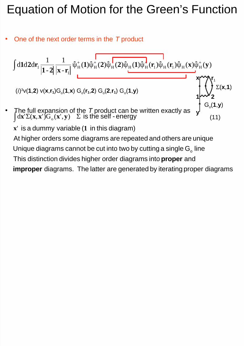
• One of the next order terms in the T product

• The full expansion of the T product can be written exactly as

(i)3v(1,2) v(x,r1)Go(1,x) Go(r1,2) Go(2,r1) Go(1,y)

)(ψ)(ψ)(ψ)(ψ)(ψ)(ψ)(ψ)(ψ-

1

-

1ddd HH1H1HHHHH

1

1 yxrr1221rx21

r21 ++++∫

(11)

Go(1,y)

y

1

x

Σ(x,1)

2

r1

diagramsproperiteratingbygeneratedarelatterThe diagrams.

andintodiagramsorderhigherdividesndistinctioThis

lineGsingleacuttingbytwointocutbecannotdiagramsUnique

uniqueareothersandrepeatedarediagramssomeordershigherAt

diagram)thisin (variabledummyais

energy-selftheis

o

improper

proper

1x

yxxxx

'

),'()G',('d o ΣΣ∫




• The proper self-energy Σ* (F 105, M 181)• The self-energy has two arguments and hence two ‘external ends’• All other arguments are integrated out

• Proper self-energy terms cannot be cut in two by cutting a single Go

• First order proper self-energy terms Σ*(1)

• Hartree-Fock exchange term Hartree (Coulomb) term

Exercise: Find all proper self-energy terms at second order Σ*(2)

r1

x

x’ (10)(9)x’

x

i f i f h i




• Equation of Motion for G and the Self Energy

[ ]

potentialncorrelatio-exchangetheis

heresuppresseddependencetime

indirectputtoisphysicsmattercondensedinConvention

direct

exchangedirect

)',(

,,

)-(),'(G)',('d),G(Vht

)',(V)',()',(

H )(

)',(V),(G)'('1d)',)((

)()(

),'(G)',('d)(ψ)(ψ)(ψ)(ψ1

d

1

oH

H

o)1(

H11o

1

1)1(

)1()1()1(

ooHH1H1Ho

1

1

xx

ryx

yxyxxxxyx

xxxxxx

xxrrxxrx

rxx

yxxxxyxrrrx

r

∑

=∑+

−−

∂∂

−∑→∑

∑

=−−=∑

∑+∑=∑

∑=ΨΨ−

∫

∫

∫ ∫ ++

δ

δ

ii

iT i

i f i f h i




• Dyson’s Equation and the Self Energy

),''(G)'','()',(G''d'd),(G),G(

VH H

)-(),(GVht

)-(),'(G)',('d),G(Vht

ooo

Ho

oH

oH

EquationsDyson'

)incl.( systemginteractin-nonforGforMotionofEquation

systemginteractinforGforMotionofEquation

o

yxxxxxxxyxyx

yxyx

yxyxxxxyx

∫ ∫

∫

∑+=

=

=

−−

∂∂

=∑+

−−

∂∂

δ

δ

i

ii

E i f M i f h G ’ F i




• Integral Equation for the Self Energy

equationsDyson'inbyreplacemay weHence

andusing

andCompare

energyselfpropertheiteratingbygenerated

energyselftheinterms(repeated)improperi.e.

byrelatedareenergyselfpropertheandenergy-selfThe

GG

GGGGGGG

GGGGGGG

GGGGG

),')G(',('d ),'()G',('d

...GGG

)','''()''',''()G'',('''d''d)',()',(

*

o

o

*

o

*

o

*

o

*

o

*

o

**

o

*

o

*

o

*

o

*

o

*

o

*

o

o

**

ooo

*o

*

o

*

o

**

o

**

o

**

*

ΣΣ

+ΣΣΣ+ΣΣ+Σ=Σ

+ΣΣΣ+ΣΣ+Σ=Σ

ΣΣ+Σ=ΣΣ+=ΣΣ

+ΣΣΣ+ΣΣ+Σ=Σ

ΣΣ+Σ=Σ

ΣΣ

∫ ∫

∫∫

yxxxxyxxxx

xxxxxxxxxxxx



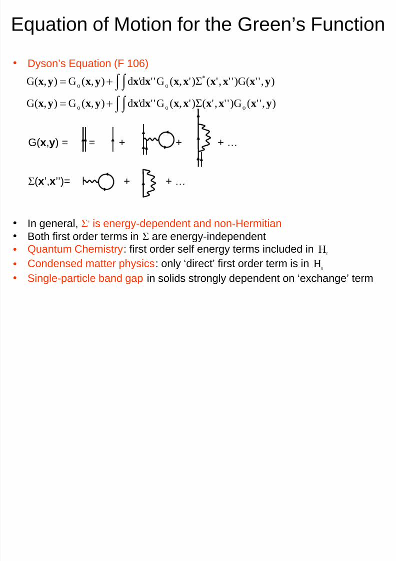
• Dyson’s Equation (F 106)

• In general, Σ∗ is energy-dependent and non-Hermitian• Both first order terms in Σ are energy-independent

• Quantum Chemistry: first order self energy terms included in Ho

• Condensed matter physics: only ‘direct’ first order term is in Ho

• Single-particle band gap in solids strongly dependent on ‘exchange’ term


∫ ∫ ∫ ∫

Σ+=

Σ+=

),''()G'','()',(G''d'd),(G),G(

),'')G('','()',(G''d'd),(G),G(

ooo

*

oo

yxxxxxxxyxyx

yxxxxxxxyxyx

G(x,y) = = + + + …

Σ(x’,x’’)= + + …



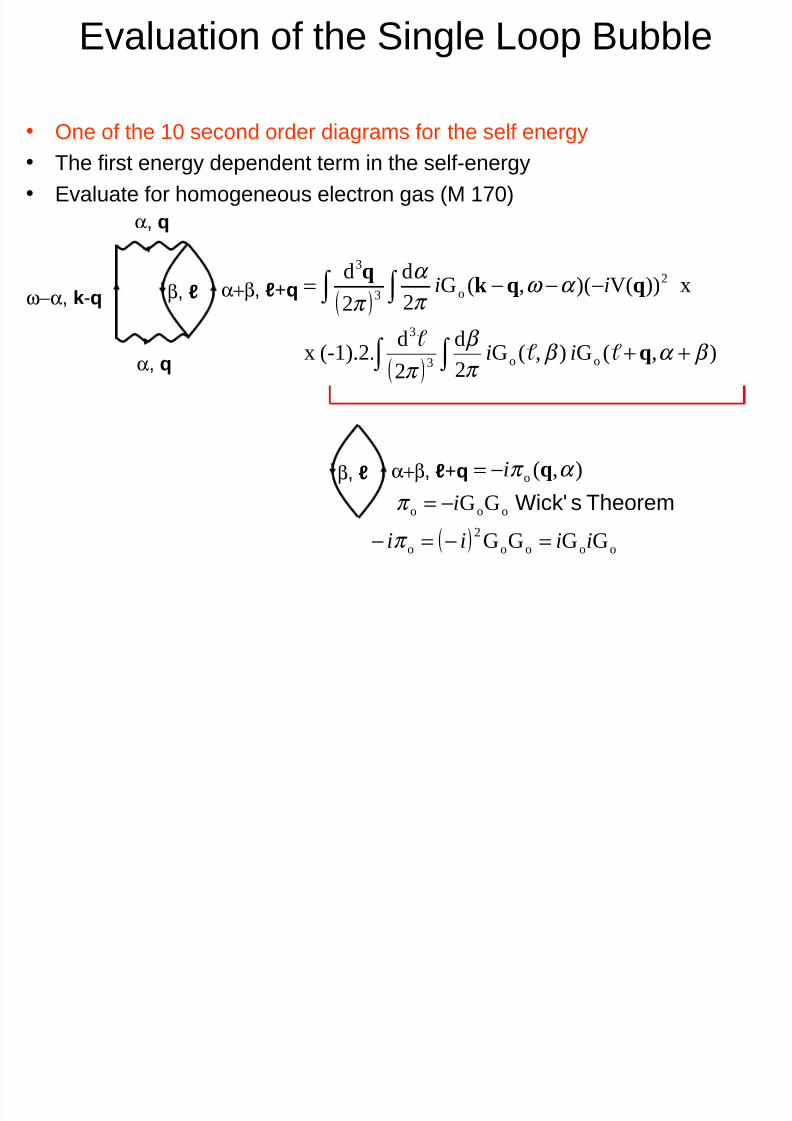
• One of the 10 second order diagrams for the self energy• The first energy dependent term in the self-energy

• Evaluate for homogeneous electron gas (M 170)

Evaluation of the Single Loop Bubble

( )

( )

( ) oooo

2

o

ooo

o

oo3

3

2o3

3

GGGG

GG

),(

),(G),(G2

d

2

d(-1).2.x

x))V((),(G2d

2d

iiii

i

i

ii

ii

=−=−

−=−=

++

−−−=

∫ ∫

∫ ∫

π

π

α π

β α β π

β

π

α ω π α

π

TheoremsWick'

q

q

qqkq

α+β, ℓ+qβ, ℓ

α+β, ℓ+qβ, ℓω−α, k-q

α, q

α, q



•Polarisation bubble: frequency integral over β

• Integrand has poles at β = ε ℓ - iδ and β = -α + ε ℓ+q + iδ

• The polarisation bubble depends on q and α

• There are four possibilities for ℓ and q


δ ε α β β α

δ ε β β

β α β π

β

i

ii

i

ii

ii

±−+=++

±−=

++

+

∫

q

q

q

),(G ),(G

),(G),(G2

d

oo

oo

FF

FF

FF

FF

kqk

kqk

kqk

kqk

>+<

<+<

>+><+>

x

y

δ ε α β i++−= +q

δ ε β i−=

FF kqk <+>



•Integral may be evaluated in either half of complex plane


x

y

δ ε α β i++−= +q

δ ε β i−=

FF kqk <+>

( )0

1

ee2

ed

2

d

2

lim

=∝∝

=+=

∫ ∫

∫ ∑∫ ∫

∞→

−

∞

∞

−

rr

i

r

ir

i

ii

i

rφ φ

φ

π π

β

π planehalfupperincirclesemi

-planehalfUpper

clockwiseAnti residues

( )( )

[ ]( )ba

1

bzaz

1f(z)

−=→

−−=

azatf(z)residue

( )

( )

( )

δ ε ε α δ ε δ ε α

δ ε α β δ ε α β δ ε β

i

i

ii

i

ii

i

i

i

+−+−=

−−++−=

++−=

−−++−

++

++

qq

q

q

22

atpoleforresidue



• From Residue Theorem

• Exercise: Obtain this result by closing the contour in the lower half plane


δ ε ε α

δ ε ε α π

π β α β

π

β

i

i

i

iii

−+−

=

+−+−−

=++

+

+∫

q

q

q

1

2

2),(G),(G

2

doo

l i h i l bbl



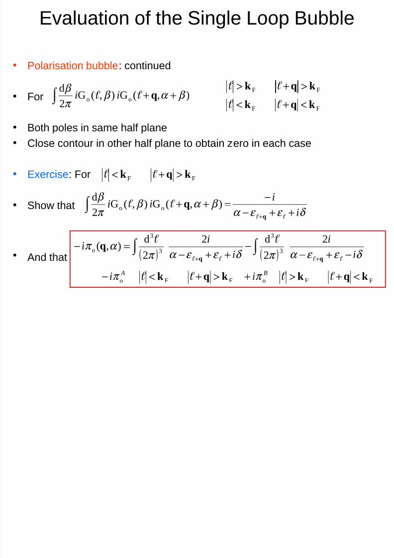
• Polarisation bubble: continued

• For

• Both poles in same half plane

• Close contour in other half plane to obtain zero in each case

• Exercise: For

• Show that

• And that


FF kqk >+<− A oiπ

FF

FF

kqk

kqk

<+<

>+>

δ ε ε α β α β π

β

i

i

ii ++−−

=++ +∫

qq ),(G),(G2

doo

( ) ( ) δ ε ε α π δ ε ε α π α π

i

i

i

ii

−+−−

++−=−

++∫ ∫

qq

q2

2

d2

2

d),(

3

3

3

3

o

FF kqk <+>+ Boiπ

),(G),(G2

doo β α β

π

β ++∫ q ii

FF kqk >+<

l i f h i l bbl



( ) ( )

( )( )

( )( )

( ) ( )

planehalflowerinpolesbothotherwisebemust

andatpoles

F

2

3

3

3

3

A

o

2

3

3A

B

o

A

o

2

3

3

oo3

32

o3

3

εεε

εε

2

ε)V(

2

d

2

d

2

d

),(ε

)V(2

d

2

d

),(),())V((ε

2

d

2

d

),(G),(G2

d

2

d))V((),(G

2

d

2

d-2

kqk

qq

qqq

qqqq

qqqkq

qqkqk

qqkqk

qkqk

qkqk

>−

−−=±−=

++−±−−=

−±−−

=Σ

+−−±−−

=

++−−−=Σ

+−−

+−−

−−

−−

∫ ∫ ∫

∫ ∫

∫ ∫

∫ ∫ ∫ ∫

δ α δ ω α

δ α δ α ω π

α

π π

α π δ α ω π

α

π

α π α π δ α ω π

α

π

β α β π

β

π α ω

π

α

π

ii

i

i

i

i

ii

i

iiii

i

iiii

• Self Energy


FF kqk >+<

β, ℓω−α, k-q

α, q

α, q

α+β, ℓ+q

E l i f h Si l L B bbl



( ) ( )

( ) ( )

dependentvector waveandenergyisenergySelf

atresidue

δ ω π π

δ ω π π

δ ω

δ ω α δ α δ α ω

iii

iii

i

ii

i

i

i

−−−+−=Σ−

+−−+−=Σ−

>>+<+−−+

−=

+−→

++−+−−

−−

−+

−+

−+−

∫ ∫

∫ ∫

qkq

qkq

qkq

qk

qqk

qq

qq

kq-kkqk

εεε

1)V(

2

d

2

d2

εεε

1)V(

2

d

2

d2

,,

εεε

2

εεε

2

ε

2

3

3

3

3B

2

3

3

3

3A

FFF

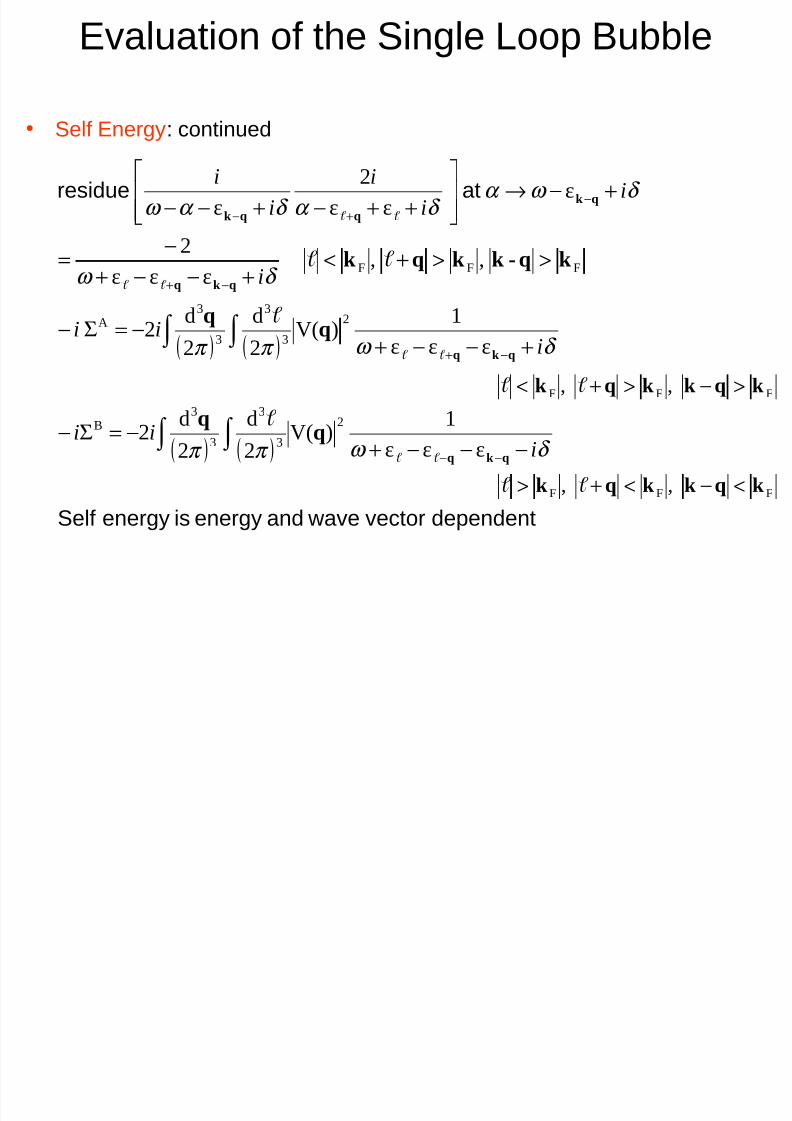
• Self Energy: continued


FFF , , kqkkqk >−>+<

FFF , , kqkkqk <−<+>

E l i f h Si l L B bbl



• Real and Imaginary Parts

• Quasiparticle lifetime τ diverges as energies approach the Fermi surface

( ) ( )

( ) ( )( )

( ) 2A1

2

3

3

3

3A

2

3

3

3

3A

ε)Im(

εεε)V(2

d

2

d 2)Im(

εεε

1)V(

2

d

2

d 2)Re( P

Σ

−−+−=Σ

−−+=Σ

−+

−+

∫ ∫

∫ ∫

ωτ

ω δ π π

π

ω π π

qkq

qkq

qq

qq


1lecturefromx

/)x( )a(

aa

1Im

a

1

a

a

a

1Re

a

a

a

1

22

lim

02

2

2

ε

π ε δ δ π

δ

δ

δ

δ δ

δ

δ

δ

ε +=−=

+−=

+

=+

=

+

+−

=+

→i

Pi

i

i

Date post:	03-Apr-2018
Category:	Documents
Upload:	gokaran-shukla
View:	218 times
Download:	0 times

Many_Body_Lecture_3.pdf

Documents