Statistical Methodology 3 (2006) 42–54 www.elsevier.com/locate/stamet MAOSA: A new procedure for detection of differential gene expression Greg Dyson a,∗ , C.F. Jeff Wu b a Department of Human Genetics, University of Michigan, Ann Arbor, MI 48109, USA b School of Industrial and Systems Engineering, Georgia Institute of Technology, Atlanta, GA 30332-0205, USA Received 5 March 2005; received in revised form 24 August 2005; accepted 25 August 2005 Abstract Gene expression data analysis provides scientists with a wealth of information about gene relationships, particularly the identification of significantly differentially expressed genes. However, there is no consensus on the analysis technique that will solve the inherent multiplicity problem (thousands of genes to be tested) and yield a reasonable and statistically justifiable number of differentially expressed genes. We propose the Multiplicity-Adjusted Order Statistics Analysis (MAOSA) to identify differentially expressed genes while adjusting for the multiple testing. The multiplicity problem will be eased by performing a Bonferroni correction on a small number of effects, since the majority of genes are not differentially expressed. c 2005 Elsevier B.V. All rights reserved. Keywords: Microarray; Multiplicity; Order statistics 1. Introduction High-throughput gene expression data has enabled scientists to simultaneously study a large number of gene effects via spotted glass arrays and oligonucleotide gene chips. However, there is no consensus on the choice of technique to analyze these data that will solve the multiplicity problem and yield a reasonable and statistically justifiable number of differentially expressed genes. A multiplicity problem arises whenever more than one hypothesis test is conducted. When conducting 100 hypothesis tests at the 0.05 level, we should expect 5 tests to be rejected even if all the null hypotheses are true. The Multiplicity-Adjusted Order Statistics Analysis (MAOSA) algorithm proposed here approaches the problem by first transforming t -like statistics to the ∗ Corresponding author. E-mail addresses: [email protected] (G. Dyson), [email protected] (C.F. Jeff Wu). 1572-3127/$ - see front matter c 2005 Elsevier B.V. All rights reserved. doi:10.1016/j.stamet.2005.08.003
MAOSA: A new procedure for detection of differentialgene expression
Greg Dysona,∗, C.F. Jeff Wub
aDepartment of Human Genetics, University of Michigan, Ann Arbor, MI 48109, USAb School of Industrial and Systems Engineering, Georgia Institute of Technology, Atlanta, GA 30332-0205, USA
Received 5 March 2005; received in revised form 24 August 2005; accepted 25 August 2005
Keywords: Microarray; Multiplicity; Order statistics
1. Introduction
High-throughput gene expression data has enabledscientists to simultaneously study a largenumber of gene effects via spotted glass arrays and oligonucleotide gene chips. However, thereis no consensus on the choice of technique to analyze these data that will solve the multiplicityproblem and yield a reasonable andstatistically justifiable number of differentially expressedgenes. Amultiplicity problem arises whenever more than one hypothesis test is conducted. Whenconducting 100 hypothesis tests at the 0.05 level, we should expect 5 tests to be rejected even ifall the null hypotheses are true. The Multiplicity-Adjusted Order Statistics Analysis (MAOSA)algorithm proposed here approaches the problem by first transformingt-like statistics to the
G. Dyson, C.F. Jeff Wu / Statistical Methodology 3 (2006) 42–54 43
uniform scale. Then a unique multiple testing correction is applied to the uniform order statisticsto determine significance.
Microarrays can reveal a wealth of biological information to scientists, including differentialexpression of genes, phenotype identification and biomarker identification.However, estimationof the variability within genes and across arrays is severely limited by the typically small numberof replicates. Transformations and normalization of the raw data are typically done to accountfor some of the variability from hybridization, scanning, arrays, etc. In general, there is a three-step process to convert raw expression data into a usable format. The raw data is initiallycorrected for background noise to eliminate systematic chip (or slide) biases. Log or square-roottransformations are often done at this stage to bring in extremely large values. Then normalizethe chips (or slides) to put them on the same scale.Often these first two steps are combined intoone step, i.e., the normalization includes background correction. Finally, the data is summarizedacross different replicates into a test statistic. Robust methods are employed to derive a teststatistic due to outliers and the inherent noisiness of gene expression data. Recent research hasemployed robust measurement in different stages of gene expression data analysis including:image analysis [12], gene filtering [8] and clustering methods [5,7].
The data set to illustrate MAOSA is derived from a large-scale analysis from [10]. Theyconducted a mixing experiment using oligonucleotide gene chips involving three groups ofhuman fibroblast cells, with six replicates in each group. The three groups of cells are serumstarved, serum stimulated and a 50/50 mixture of starved/stimulated. For the analysis in thispaper, we compare the serum starved cells versus the mixture of starved/stimulated cells.
Other standard microarray analysis techniques are described here briefly. See the originalpapers for details. Dudoit et al. [4] proposed applying the Westfall–Young (WY) step-downtechnique [17] to replicated microarray data to adjust for the thousands of comparisons. TheWY technique controls family-wise error rate (i.e., probability of at least one error in the family)in the strong sense (control for all possible combinations of true and false hypotheses). Tusheret al. [16] developed the Significance Analysis of Microarrays (SAM) procedure using at-likestatistic and permutation techniques. The authors use the False Discovery Rate (FDR) to calibratethe finalnumber of significant effects.
2. Methods
2.1. Normalization for oligonucleotide gene chips
Slide effects, image effects, and hybridization effects, etc., are not of direct interest toscientists, but play a vital role in microarray analysis. The raw data from a spotted glass arrayor a gene chip should not be directly analyzed due to these biases. Instead, analysis ought totake place on transformed (as known as normalized) data that eliminates systematic effects fromprocessing, hybridization, scanning, etc.
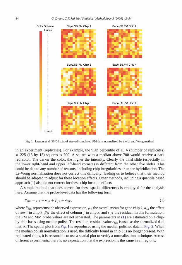
For gene chips, the Li and Wong [11] normalization is often usedif the probe level data areavailable. In general, this normalization works well to eliminate probe level biases. However, ifone examines a spatial plot of gene expression, then one would see that sometimes slide effectsare not being accounted for. The Lemon et al. 50/50 mix of the starved/stimulated PM datais used inFig. 1 to illustrate a problem that can occur if there is a bad slide. Each of the 225squares represents an area of about 625 probes on each slide (25 probes by 25 probes). Thecolors are determined by the median expressionof all probes within each square, relative to theempirical quantiles of the overall distribution of those median expression levels across all slides
44 G. Dyson, C.F. Jeff Wu / Statistical Methodology 3 (2006) 42–54
Fig. 1. Lemon et al. 50/50 mix of starved/stimulated PM data, normalized by the Li and Wong method.
in an experiment (replicates). For example, the 95th percentile of all 6 (number of replicates)× 225 (15 by 15) squares is 700. A square with a median above 700 would receive a darkred color. The darker the color, the higher the intensity. Clearly the third slide (especially inthe lower right-hand and upper left-hand corners) is different from the other five slides. Thiscould be due to any number of reasons, includingchip irregularities or under-hybridization. TheLi–Wong normalization does not correct this difficulty; leading us to believe that their methodshould be adapted to adjust for these location effects. Other methods, including a quantile basedapproach [1] also donot correct for these chip location effects.
A simple method that does correct for these spatial differences is employed for the analysishere. Assume that the probe-level data has the following form
Yi jk = µk + αik + β j k + εi j k , (1)
whereYi jk represents the observed expression,µk the overall mean for gene chipk, αik the effectof row i in chipk, β j k the effect of columnj in chipk, andεi j k the residual. In this formulation,the PM and MMprobe values are not separated. The parameters in(1) are estimated on a chip-by-chip basis using median polish. The resultant residual valueεi j k is used as the normalized datamatrix. The spatial plot fromFig. 1is reproduced using the median polished data inFig. 2. Whenthe median polish normalization is used, the difficulty found in chip 3 is no longer present. Withreplicated chips, it is reasonable to use a spatial plot to verify a normalization technique. Acrossdifferent experiments, there is no expectation that the expression is the same in all regions.
G. Dyson, C.F. Jeff Wu / Statistical Methodology 3 (2006) 42–54 45
Fig. 2. Lemon et al. 50/50 mix of starved/stimulated, normalized with median polish.
2.2. Summary value for each gene within one slide
After normalization, the next step is to summarize the PM and MM probe values into onenumber for each gene. For each of the 7129 genes (or probe sets) on the gene chip, there areapproximately 20 PM and MM probe pairs. Therefore for each gene, the expression within eachchip is defined as
τi = Medianj {PMi j − MM i j }, (2)
for i = 1, . . . , 7129, j = 1, . . . , Ni , whereNi is the number of probes in probe set (or gene)i .There exists one number for each gene in each experiment.
Alternatively, an analysis on the PM-only data may be employed. This would entail usingτi = Medianj {PMi j } as the test statistic instead of(2). It is still debatable whether the MMprobes any utility. Cope et al. [2] were unable to conclude that the MM values provide any utility.Irizarry et al. [9] suggested that “the MMs are a mixture of probes for which (i) the intensities arelargely due to non-specific bindingand background noise and (ii) the intensities include transcriptsignal just like the PMs”. Since the MM probes are in some instances measuring actual signal orbinding,discarding them will cause a loss of information. There is no “best” way to utilize theMM probes, but a simple difference in medians should alleviate some concern.
2.3. Calculate a teststatistic for each gene across replicates
For a replicated comparable gene chip experiment, construct the two-samplet-statistic as thetest statistic for thel th gene (l = 1, . . . , n), using robust measures instead of the mean and
46 G. Dyson, C.F. Jeff Wu / Statistical Methodology 3 (2006) 42–54
In (3), τi,k refers to the vector of summary values for genei in condition k (k = 1, 2)
from the replicated experiments,ni,k is the number of replicates for conditionk (k = 1, 2)
andc is a constant included to insure that genes that merely have low variability across samplesare not mistakenly called significant. The normalization should have eliminated the systematicbiases that exist in the experiment, so the median and median absolute deviation (MAD) arereasonable and consistent estimates of the location and scale for each gene effect. Noting thatthere are typically a small number of replicates in a microarray experiment, we choose theserobust measures since outliers in the data affect them less than the mean and standard deviation.Other papers have suggested criteria for choosing such ac, including the minimization of thecoefficient of variation [16] andusing the 90th percentile of the rest of the denominator [6]. Thesecorrection methods lack a strong statistical justification. In the next section, a different methodfor determiningc is described that is based on the normality assumption about the statistics in(3).
2.4. Determine c using the first four moments of the normal distribution
This analysis will not make the strong assumption that the rtsi (3) follow a normal distribution.Instead, we willassume that itsmiddle portion follows a normal distribution. Therefore it isnecessary to determine the expressions for the first four moments of the normal distributionwhen data from the upper and lower tails are truncated. LetX ∼ N(µ, σ 2). DefineY = {X :a < X < b}. DefineΦ(x, y, z) as the cumulative distribution function of a normal with meany and standard deviationz evaluated atx andφ(x, y, z) as the density of a normal distributionwith meany and standard deviationz evaluated atx. It can be shown that
G. Dyson, C.F. Jeff Wu / Statistical Methodology 3 (2006) 42–54 47
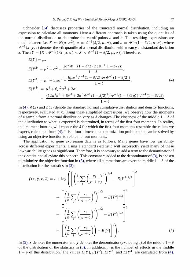
Schneider [14] discusses properties of the truncated normal distribution, including anexpression to calculate all moments. Here a different approach is taken using the quantiles ofthe normal distribution to determine the cutoff pointsa and b. The resulting expressions aremuch cleaner. LetX ∼ N(µ, σ 2), a = Φ−1(δ/2, µ, σ ), andb = Φ−1(1 − δ/2, µ, σ ), whereΦ−1(x, y, z) denotes thexth quantile of a normal distribution with meany and standard deviationz. ThenY = {X : Φ−1(δ/2, µ, σ ) < X < Φ−1(1 − δ/2, µ, σ )}. Therefore,
In (4), Φ(x) andφ(x) denote the standard normal cumulative distribution and density functions,respectively, evaluated atx. Using these simplified expressions, weobserve how the momentsof a sample from a normal distribution vary asδ changes. The closeness of the middle 1− δ ofthe distribution to what is expected is determined, in terms of the first four moments. In reality,this moment-hunting will choose theδ for which the first four moments resemble the values weexpect, calculated from(4). It is a four-dimensional optimization problem that can be solved byusing an objective function to relate the four moments.
The application to gene expression data is as follows. Many genes have low variabilityacross different experiments. Using a standardt-statistic will incorrectly yield many of theselow variability genes as significant. Therefore, it is necessary to add a term to the denominator ofthet-statistic to alleviate this concern. This constantc, added to the denominator of(3), is chosento minimize the objective function in(5), where all summations are over the middle 1− δ of thedistribution forthe statistics in(3):
f (x, y, c, δ) = c + log
(
1
n
∑i
(xi
yi + c
)4)1/4
− E[Y4]1/4
2
+(1
n
∑i
(xi
yi + c
)3)1/3
− E[Y3]1/3
2
+(
1
n
∑i
(xi
yi + c
)2)1/2
− E[Y2]1/2
2
+[(
1
n
∑i
(xi
yi + c
))− E[Y]
]2 . (5)
In (5), x denotes the numerator andy denotes the denominator (excludingc) of themiddle 1− δ
of the distribution of the statistics in(3). In addition, n is the number of effects in the middle1 − δ of this distribution. The valuesE[Y], E[Y2], E[Y3] and E[Y4] are calculated from(4).
48 G. Dyson, C.F. Jeff Wu / Statistical Methodology 3 (2006) 42–54
The first term in(5) is included so that smaller values ofc are selected. It is not our goal tohavec dominate the denominator of(3), but rather to ensure that genes with low variabilityacross the experiments are not mistakenly declared to have significant differential expression.This method is aimed at detectinglarge significant effects. The interest is not to locatesmalltranscript variability that may be biologicallyimportant. Use of the roots corresponding to thedegree of moments (e.g.,1
2 for the second moment) in(5) puts the expressions of the fourmoments on the same scale. In addition, log is taken to make it easier to distinguish betweendifferent values ofc and limit the effect that the first term will have on the chosenc. Eq. (5) issimply an adaptation of the classic “observed minus expected squared minimization” techniquefound in goodness-of-fit tests, for example. This choice ofc will ensure that the middle 1− δ
of the test statistic is normally distributed. Other correction methods (including no correction atall) will just assume this conclusion without testing its validity. By forcing the majority of thegene expressions to follow a normal distribution, we have an estimated distribution on which theinference is made.
A numerical minimization procedure is used to solve forc. It is necessary to input the valuesof µ andσ 2 in order to computeE[Y], E[Y2], E[Y3], E[Y4] in (4) for use in(5). To avoideven a slight effect of outliers, the median of the input vector (i.e., setc = 0 in (3)) is used as theestimate forµ, while the MAD is used as the estimate forσ . This criterion for selectingc ensuresthat 1− δ of the distribution of the statistics in(3) will mimic a normal distribution. Implicitlythis assumes that 1− δ of this distribution is not differentially expressed.
For different values ofδ, theoptimal c is calculated. The final selection ofδ will depend onthe priorknowledge of the experimenter and the resultant minimum value. One can examine aplot of δ versusc versus the minimum value to see where theoptimal regions are.
For the Lemon et al. starved versus starved/stimulated data, the minimum value attaineddepends mostly onδ. Fig. 3 displays two plots which relatedδ to c and the minimum valueattained. A loess smoother was added to the plots to help visualize the distribution. The constantc does not seem to be an important component in the determination of the minimum value. Bothsmoothing curves obtain a minimum value at aroundδ = 0.10. At thatδ, c = 1.92, with aminimum value of−9.73. Thisis thec used in(3) to compute the test statistics used in the laterstages of the analysis. Note that thisδ assumes that approximately 90% of the gene effects arenull. Fig. 4 demonstrates the difference between the distribution of the test statistics(3) withno adjustment(c = 0) and the adjustment set forth in this section(c = 1.92) for the Lemonet al. data. From the right-hand picture, it appears that the adjustment has achieved its purpose offorcing the middle 1− δ = 90% of the data to mimic a normal distribution. Using no adjustmentwill yield a more curvilinear distribution in the middle part (between−2 and 2 on thex-axis) ofthe distribution of(3).
2.5. Analysis using beta statistics
An analysis can be done using a well-known fact regarding order statistics. Suppose we have asampleXi , i = 1, . . . , n from a distribution functionF . It isknown from the probability integraltransformation (PIT) thatF(Xi ), i = 1, . . . , n, areuniformly distributed over(0, 1). In essence,a random sample from any distribution function can be converted to a uniform(0, 1). In additionF(X(i )), i = 1, . . . , n, has a beta distribution with parametersi andn− i +1 [3]. Since there arenice properties when using uniform order statistics, results below will only be concerned withthe standard uniform density, although the resultsare applicable to any distribution because ofthe PIT.
G. Dyson, C.F. Jeff Wu / Statistical Methodology 3 (2006) 42–54 49
Fig. 3. Optimalc determination based on(4) for Lemon et al. data.
Fig. 4. Comparison ofthe distribution of the test statistics in(3) usingc = 0 or c = 1.92.
50 G. Dyson, C.F. Jeff Wu / Statistical Methodology 3 (2006) 42–54
The joint distribution of the order statistics of a random variable can be determined. Inparticular let X1, . . . , Xn be independent and identically distributed random variables from anabsolutely continuous distribution functionF . Denote the order statistics asX(1), . . . , X(n). ForX ∼ F , David [3] showed thatF(X(s)) − F(X(r )) ∼ Beta(s − r, n − (s − r ) + 1). Thereforethe distribution of the difference in uniformorder statistics depends only on the length of thedifference, and not on the particular order statistics being subtracted. A crucial element is thecorrect distribution functionF . Hence, any analysis should include a method, like inSection 2.3to ensure that the data mimics a known distribution.
Based on these distributional results, a test canbe developed to determine change points inorder statistics. In a sense, the following procedure will identify the point at which the ordereddata shifts away from the uniform distribution. In the case of gene expression data, this procedurewill allow the identification of gene effects that are significantly different from the large amountof unexpressed genes.
2.6. MAOSA outline
A new procedure for detecting differential expression, calledMultiplicity-Adjusted OrderStatistics Analysis(MAOSA), is proposed. It consists of the following steps:
(i) Determine the optimalc and calculate the summary statistics in(3) as discussed inSection 2.4.
(ii) Convert the test statistics from (i) to the uniform scale, assuming that they have a normaldistribution. Use the median and MAD of the test statistics as the mean and standarddeviation in the probability integral transformation.
(iii) Compute test statistics using the uniform statistics derived in (ii) and setr = 1, i.e., compareeach subsequent order statistic to the minimum order statistic. This analysis is two-sided inthat it looks for significance in both the upper and lower tails.
(iv) Compare the test statistics from (iii) to the theoretical beta quantiles. When making thiscomparison, use the Bonferroni correction on a small number effects since the majority ofgene effects can be ignored.
(v) Determine the segments of genes that have significant differential expression.
Note that an alternative normalization technique or test statistic may be employed in the earlystages of this algorithm. However, after step (i) it is necessary that the gene summary statisticshave a known distribution (in this case, normal) toproceed with the algorithm. There are a host ofother methods to ascertain statistical significance of normally distributed statistics, from a simplep-value from at-distribution to non-parametric methods. The proposed method is compared tothe SAM and WY methods introduced inSection 1.
The Bonferroni adjustment employed in step (iv) works in the following way. First, eliminateeffects that are clearly notsignificant. The choice ofc allows us to ignore the vast majority ofeffects. Since we assume that the test statistic has a normal null distribution, effects that fallwithin ±2 s.d. should not be declared significant. Hence, the Bonferroni adjustment is employedonly when we move past those null effects as we have helped define by the selection ofc. Teststatistics from (iii) that do not pass a non-correctedp-value (say, 0.10) cutoff are excluded.This cutoff should be no less than theδ chosen to lessen the possibility of a type II error.There are effects left in the lower and upper tails. For the effects in the upper tail, start at thesmallest indexed order statistic remaining and determine the first occurrence ofr consecutivesignificant genes. A similar procedure is done for the remaining genes in the lower tail. In this
G. Dyson, C.F. Jeff Wu / Statistical Methodology 3 (2006) 42–54 51
phase, ther comparisons are adjusted via the Bonferroni correction, i.e., use levelα/r . Theselection of this smallnumber,r , will depend on the data and the expected number of significanteffects. For example, there are 7129 genes in the Lemon et al. data. There were 1199 genesthat passed the initial screening, with 61 in the lower tail and 1138 in the upper tail. Next, startat the smallest index of the 1138 order statistics in the upper tail, in this case, order statisticnumber 5992. Starting from this order statistic, find the firstr consecutive ordered test statisticsthat pass the Bonferroni corrected significance level. All subsequent test statistics (after theinitial r significant) are also declared significant. Oncesome ordered effects are significant, thesubsequent (i.e., larger) effects are also significant. The same logic is used in half-normal plotsfor detecting significance in factorial experiments. (For details on half-normal plots, see [18]).Table 1displays the results for the Lemon et al. data, usingr = 10. The first column (α) indicatesthe significance level employed, the second column (# Significant) the number of significanteffects, and the third column the FDR. This example is further discussed inSection 3.
Other test statistics were considered in step (iii) of the above algorithm, including comparingall order statistics to the maximum order statistic. In addition, Stephens [15] suggested using
Z = (n − i + 1)U(i )
i (1 − U(i )), (6)
which has anF2i,2(n−i+1) distribution. However, we chose to use the proposed technique due toits simplicity and nice distributional properties.
3. Results
The analysis presented in this section compares the cells grown in the starved environmentto those grown in the mixed starved/stimulated environment from the Lemon et al. data cited inSection 1. We follow the procedure outlined inSection 2for the data pre-processing. For thisexample, usingδ = 0.10 in (4) yields c = 1.92 in (3). Using this δ value tacitly assumes thatabout 10% of the data is differentially expressed. Some methods for determining differentialexpression as well as methods for assessing the validity of such an analysis require permuteddata sets. Therefore set thec for test statistics computed from the permuted data sets to be 1.92.This reduces the bias by keeping the permuted data on the same level as the original.
Continuing with the outline fromSection 2.6, the teststatistics are converted to the uniformscale using PIT. These uniform statistics are used to produce beta test statistics. Then using a two-sided hypothesis test, calculatep-values for each test statistic versus its respective theoreticalbeta distribution. Gene indices near 0 correspond to genes with the most negative value from(3),while gene indices near 7100 correspond to genes with the most positive value from(3). Geneswith the smallestp-values lie on the extremes.
The next step is to determine which genes are significant. The obvious method to use involvestheoretical quantities from the beta distribution. Since there will be multiple testing issues, a
52 G. Dyson, C.F. Jeff Wu / Statistical Methodology 3 (2006) 42–54
Fig. 5. p-values for Lemon et al. data, using the MAOSA procedure.
correction is necessary. We use theBonferroni adjustmentsince it requires no independenceassumption. However, enforcing the Bonferroni correction over 7129 tests would be impractical.Therefore, to deal with the multiplicity problem in a prudent manner, we only enforce thecorrection on a small subset of tests, in this example, 10. SeeSection 2.6for a detailedexplanation on how the Bonferroni correction was employed in this example. Ten was chosenbecause we assume that only a small number of effects would be significant based on a WYanalysis which found 7 significant effects when controlling type I error at 0.05.Table 1showsthe analysis results using MAOSA as described inSection 2.6.
The number of significant genes for this data are 975, 824, 681 and 613 for varioussignificance levelsα given inTable 1. An estimate of the error rate for each of these “significancesets” can be obtained using the FDR. Permute the condition labels while maintaining balancebetween conditions. Compute the robust statistics(3), keeping the samec = 1.92 for eachpermuted data set. Then using the sameα valuesfrom Table 1and MAOSA, compute the numberof significant effects for each permuted data set.The average number of significant genes overall 400 permuted data sets for anα value divided by the number of significant genes found bythe actual data set (for the sameα value)is the FDR.
Fig. 5 displays thep-values for the 7128 genes other than the one corresponding to theminimum order statistic. Most of the significant effects are the larger order statistics. For thisdata, it means that the significant genes are more expressed in the mixed condition rather thanthe starved.
As described above, a permutation method was used to help determine the error rates of thesets of significant effects. The FDRs for each of the sets of significant effects are listed inTable 1.With such low FDRs, 975 would be our choice for the number of significant effects. An analysisusing SAM was also done on the same data.Table 2summarizes these results. Since MAOSA hasa lower FDR forall subsets of significant effects, we believe thatit is at least comparable to SAM.
G. Dyson, C.F. Jeff Wu / Statistical Methodology 3 (2006) 42–54 53
It is necessary to explain why the error control rates for both the MAOSA and SAM are so lowwhen calling hundreds of genes significant. Pan et al. [13] postulated that the SAM method (andsimilarly the MAOSA method) assumes that under the null hypothesis no genes are differentiallyexpressed. For testing a small subset of genes, this is reasonable. However, with hundreds orthousands of tests, it may be necessary to adjust the reference distribution by adding significanteffects. Further development is needed here.
4. Discussion
A new method for identifying differentially expressed genes for oligonucleotide gene chipswas proposed in this paper. The MAOSA technique first transforms the test statistics by assumingthat the middle part of the distribution of the test statistics follows a known distribution.Then these test statistics are converted to the uniform scale, using the probability integraltransformation. Analysis thenproceeds with the uniform order statistics. To prudently correctfor multiple testing, a Bonferroni adjustmentis done on a small number of effects. This methodcan also incorporate a priori biological knowledge in the analysis with the selection ofc. Thistechnique can alsobe applied to other types of large data including spotted glass microarrays.
Acknowledgements
This research was supported in part by NSF grant DMS 0305996. The authors would liketo thank the Associate Editor and the two anonymous reviewers for their suggestions whichimproved this paper.
References
[1] B.M. Bolstad, R.A. Irizzary, M. Astrand, T.P. Speed, A comparison of normalization methods for high densityoligonucleotide array data based on variance and bias, Bioinformatics 19 (2003) 185–193.
[3] H.A. David, Order Statistics, John Wiley and Sons, New York, 1981.[4] S. Dudoit, Y.H. Yang, M.J. Callow, T. Speed, Statistical methods for identifying differentially expressed genes in
replicated cDNA microarray experiments, Statistica Sinica 12 (2002) 111–140.[5] G. Dyson, C.F.J. Wu, ICI: A new approach to explore between-cluster relationshipswith applications to gene
expression data, Georgia Tech School of Industrial and Systems Engineering — Statistics Group Technical Report,11/2005, 2005.
[6] B. Efron, R. Tibshirani, J.D. Storey, Empirical Bayes analysis of a microarray experiment, Journal of the AmericanStatistical Association 96 (2001) 1151–1160.
[7] M.A. Hibbs, N.C. Dirksen, K. Li, O.G. Troyanskaya, Visualization methods for statistical analysis of microarrayclusters, BMC Bioinformatics 6 (115) (2005).
54 G. Dyson, C.F. Jeff Wu / Statistical Methodology 3 (2006) 42–54
[8] S. Imoto, T. Higuchi, S.Y. Kim, E. Jeong, S. Miyano,Residual bootstrapping and median filtering for robustestimation of gene networks from microarray data, Computational Methods in Systems Biology Lecture Notesin Computer Science 3082 (2005) 149–160.
[9] R.A. Irizarry, B. Hobbs, F. Collin, Y.D. Beazer-Barclay, K.J. Antonellis, U. Scherf, T.P. Speed, Exploration,normalization, and summaries of high density oligonucleotide array probe level data, Biostatistics 4 (2003)249–264.
[10] W.J. Lemon, J.J.T. Palatini, R. Krahe, F.A. Wright, Theoretical and experimental comparisons of gene expressionindexes for oligonucleotide arrays, Bioinformatics 18 (2002) 1470–1476.
[11] C. Li, W.H. Wong, Model-based analysis of oligonucleotide arrays: Expression index computation and outlierdetection, Proceedings of National Academy of Science USA 98 (2001) 31–36.
[13] W. Pan, J. Lin, C. Le, A mixture model approach to detecting differentially expressed genes with microarray data,Functional and Integrative Genomics 3 (2001) 117–124.
[14] H. Schneider, Truncated and Censored Samples from Normal Populations, Marcel Dekker, Inc., New York, 1986.[15] M.A. Stephens, Tests for the uniform distribution, in: R.B. D’Agostino,M.A. Stephens (Eds.), Goodness-of-fit
Techniques, Marcel Dekker, Inc., New York, 1986.[16] V.G. Tusher, R. Tibshirani, G. Chu, Significance analysis of microarrays applied to theionizing radiation response,
Proceedings of National Academy of Science USA 98 (2001) 5116–5121.[17] P.H. Westfall, S.S. Young, Resampling-based Multiple Testing: Examples and Methods forp-value Adjustment,
John Wiley and Sons, New York, 1993.[18] C.F.J. Wu, M. Hamada, Experiments: Planning, Analysis, and Parameter Design Optimization, John Wiley and