Map Complexity: Comparison and ~ e a s u r e m e n t

Alan M. MacEachren

ABSTRACT. Visual complexity is defined in this paper as the degree to which the combination of map elements results in a pattern that appears to be intricate or involved. A test involving judgments of choropleth and isopleth map complexity yields three conclusions: (1) choropleth maps are consistently perceived as more complex than isopleth maps made from the same data; (2) the relationship between choropleth and isopleth maps can be closely described with a power function; and (3) the number of class intervals has a greater effect on complexity than does the pattern of the distribution mapped.

A measure of complexity applicable to the isopleth map as well a s choropleth can be derived, then, using the power function. Three graph theoretic measures are considered as objective mea- sures of choropleth map complexity, with correlations of 0.92 to 0.95 obtained between these measures and subjective complexity of choropleth maps. The graph theoretic measures for choro- pleth maps are then adjusted according to the power relationship observed between choropleth and isopleth subjective map complexity to yield a complexity measure for the latter map type. Similar procedures might be used to derive complexity measures for other map types.

T h e subject of thematic map complexity is one that is of wide interest in cartog- raphy. One reason for this interest is the assumption that map complexity may have an adverse effect on map effective- ness. While it is likely that, a t certain levels, complexity d ies impede map communication, i t is unlikely that all increases in map complexity will result in a corresponding decrease in effective- ness. An examination of the complex- ity-effectiveness relationship requires an understanding of both map complexity in general and the ways in which i t can be measured. Progress toward such an understanding is the goal of the present study.

Map complexity is related to both the nature of the distributions mapped and the symbolization used in representing these distributions. Because cartog- raphers have greater control over sym- bolization than over the distribution, differences in complexity among meth-

Dr. MacEachren is assistant professor in the Department of Geography, Virginia Polytechnic Institute and State University, Blacksburg, VA 24061.

ods of symbolization deserve careful at- tention. Determination of whether com- plexity differences among symbolization types exhibit consistent patterns is es- sential before drawing conclusions about the influence of these differences on the effectiveness of the symbolization. Com- prehensive analysis of map complexity requires the development of well-defined and repeatable measures of complexity for each form of symbolization consid- ered. The most useful measures would be those that can be applied to a variety of symbolization types. If consistent re- lationships exist between the subjective complexity of maps using different methods of symbolization, a physical measure of map complexity developed for maps using one method of symboliza- tion could be adapted to scale the com- plexity of maps using other methods. The specific goals of this study are to ex- amine the relationship between subjec- tive complexity of choropleth maps and shaded isopleth maps (two common methods of thematic symbolization) and, based on this relationship, to develop a physical measure of complexity that can be applied to both forms of symboliza- tion. '

The American Cartographer, Vol. 9, No. 1, 1982, pp. 31-46

DEFINITION O F MAP COMPLEXITY

The study of map complexity has been hampered by the lack of a consensus on t h e definition of t h e t e rm itself. Al- though many measures of complexity exist, they do not all measure the same thing. Differing interpretations of com- plexity have contributed to the difficulty of formulating a conceptual definition of complexity as it applies to maps. There are differences in the concept itself and there are various aspects of the map to which a concept is applied. To under- stand the variations in the concept of complexity a s applied to maps, i t is use- ful to refer to a standard dictionary defi- nition. Because complexity is generally defined a s the quality or state of being complex, it is the definition of complex tha t must be considered.

Complex: 1. composed of interconnected par ts ; compound; composite. 2 . charac- terized by a very complicated or involved combination of parts, units, etc. 3. so com- plicated as to be difficult to understand.'

These definitions represent two points of view. The first, presented in definitions 1 and 2, is concerned with the intercon- nectedness of parts. The second, repre- sented by definition 3, emphasizes ease of understanding. A somewhat different dichotomy of meaning associated with complexity is pointed out by Brophy in his statement tha t

. . . visual map complexity is tha t which is a direct consequence of the spatial differentia- tion of the graphic content of the map, while ~ntellectual map complexity is tha t which is due to the meaning or significations con- tained In or ascribed to the symbolism.'

These two aspects of map complexity, visual and intellectual complexity, are likely to influence different stages of the car tographic communication process. Visual complexity should be most im- portant in "map reading," defined by Morrison a s those processes involved with perception andlor cognition of the information on the map (detection, dis- crimination, recognition, and estima- tion). Intellectual complexity, on the other hand, should have the greatest in-

fluence on the subsequent stages of in- terpretation and analysis (interaction of information received from the map with previously held information and ad- justment of a person's cognition of real- ity as a result of this interpretation).'

I t is the visual aspect of complexity over which t he car tographer h a s the greatest control and, therefore, to which attention must first be directed. The vi- sual aspect of map complexity is related primarily to pattern geometry within t h e m a p i tself . Muehrcke probably comes the closest to expressing the es- sence of this concept in defining map complexity a s ". . . the spatial variance in map pattern. . ." measured a s ". . . the internal organization or dependence in map pattern.""

A third set of distinctions concerning the concept of map complexity is pointed out by Olson." She makes a distinction be tween complexi ty a s a n i n h e r e n t property of the distribution (dependent upon its pattern geometry but not on vi- sual judgments) and complexity a s a vi- sua l characteristic of t h e m a p (if we judge the map to be complex, i t is). Char- acteristics of the underlying distribution were used by both Muehrcke and Morri- son in the creation of a series of maps tha t varied in complexity while Olson used the map itself in her study of the relationship between measured and per- ceived complexi ty. ' A l though t h e r e should be a relationship between t he complexity of the underlying distribu- tion and the visual complexity of the map, the consistency of the relationship may depend on map type and other fac- tors.

A definition of complexity t ha t focuses on the visual characteristics of the map is adopted for purposes of th i s study. Map complexity is defined simply a s the degree to which the combination of map elements results in a pattern tha t ap- pears to be intricate or involved. In this sense, map complexity is a subjective impression formed by the map reader. Before attempting to develop a physical measure tha t approximates visual com- plexity and tha t can be adapted to both choropleth and shaded isopleth maps the

T h e American Cartographer

relationship between subjective com- plexity for these two kinds of maps will be examined. This relationship will then be used to create an index of complexity for isopleth maps tha t is based on a mea- sure that is directly applicable only to choropleth maps.

COMPARISON OF CHOROPLETH AND ISOPLETH COMP1,EXITY

Visual patterns of both choropleth and isopleth maps depend on the distribution of the data, the size, shape, and location of enumeration units. the method of data classification, and h e boundaries be- tween classes. Differences in pattern be- tween choropleth and isopleth maps re- sults from the assumption of continuity inherent in isopleth maps as well as the nature of the boundaries between sym- bols. On choropleth maps these bound- aries are usually arbitrarily defined po- litical boundaries whose specific location is not necessarily related to the distribu- tion mapped. In contrast, isopleth map boundaries are a more direct function of the underlying distribution. The bound- ar ies on choropleth maps tend to be angu la r or i r regular (which is most noticeable when individual units a r e la rge) while boundaries on isopleth maps are smooth. In addition, adjacent areas on choropleth maps can differ in value by several classes (presumably re- sulting in greater visual contrast across the map) while adjacent areas on iso- pleth maps are also adjacent in value level.

Based on t h e above cr i te r ia , i t i s hypothesized tha t choropleth maps are visually more complex t h a n isopleth maps of the same distribution. At the lowest level of complexity (a one class map) each should have a value of zero. As complexity increases, there is likely to be some level beyond which differ- ences in complexity are no longer appar- en t to an observer. A curvilinear re- lationship is therefore hypothesized, with choropleth and isopleth complexity equal a t the low and high ends of the spectrum and the most noticeable differ- ences found between these extremes (Fig. 1).

ISOPLETH COMPLEXITY

Figure 1. Hypothesized relationship between choropleth and isopleth map complexity. The range of each axis is from the minimum possible complexity to some maximum that would normally be found on maps.

Test Maps The objectives of the initial stage of

this experiment were to test the hypoth- esis that choropleth maps are more com- plex than isopleth maps and to generate a psychological scaling of complexity to which physical measures can be com- pared. Methods for creating a psycholog- ical complexity continuum share one re- qu i r emen t : t h a t a l a rge sample of stimuli covering a broad range of values be presented to the subjects. To obtain a sufficient range of stimuli, eighty maps, forty choropleth and forty isopleth, were produced.

All maps used in the test have the same base ( a section of contiguous U.S. counties chosen to be representative of areas with irregular boundaries). The base map selected has sixty enumera- tion units and is a section of a county map of central Kentucky (Fig. 2). The area represented was mapped a t an un- conventional orientation to minimize the possibility tha t impressions of com- plexity will be influenced by familiarity with the area. The mapped area was de- fined by a rectangular boundary.

The distributions to be mapped were chosen to represent a broad range of typ- ical geographical distributions. Ten dis- tributions representative of a range of

Vol. 9, No. 1 , April 1982

Figure 2. The base map.

socio-economic, agricul tural , and cli- matic data were used. Maps with two, three, four, and five classes were pro- duced. Although two-class maps are not commonly encountered, they a r e in- cluded in this study to extend the range of complexity and achieve more accurate scaling.

The maximum number of classes is re- stricted to five in light of the perceptual "rule" tha t the average person can easily distinguish only about five shades of gray.x Many classification techniques exist by which data may be grouped. In relation to visual map complexity

a major difference in these classifica- tion systems is t h a t they will resul t in different numbers of units in each class. To control for this variable. all data were classed in quantiles, thus re- sulting in an equal number of unit val- ues in each class. Maps were produced without scales or legends.

For each of the ten distributions, two-, three-, four-, and five-class choropleth and isopleth maps were created yielding a total of forty of each kind of map. On choropleth maps, boundary lines be- tween enumerat ion uni t s with equal values were omitted. Using the visual centroids of the enumeration units a s control points, isolines on the isopleth map were drawn using the Surface I1 Graphics S y s t e m . T h e two- through five-class choropleth-isopleth pairs for one of t he ten distributions a r e pre- sented in Figs. 3-6 respectively.

Methodology The initial procedure was to deter-

mine the subjective complexity of the test maps. This was accomplished by generating a psychological complexity scale to which physical complexity mea- sures for each map could subsequently be com~ared .

~ s ~ c h o ~ h ~ s i c a l scaling techniques can be categorized a s direct or indirect. With indirect scaling, the step between the

Figure 3. Two-class cho~

34

ropleth-isopleth map pair.

The American Cartographer

Figure 4. Three-class choropleth-isopleth map pair.

Figure 5. Four-class choropleth-isopleth map pair

Figure 6. Five-class choropleth-isopleth map pair.

Vol. 9, No. 1, April 1982

raw data and the final scale involves the application of a hypothetical psychologi- cal dimension to convert the ordinal data to interval scale data.1° Alterna- tively, direct scaling minimizes the steps between the raw data and the final scal- ing by defining, in the instructions to the subjects, the quantitative property to be measured. Operationally, there- fore, direct scaling can be more easily applied and should produce more accu- rate results when a particular character- istic such as complexity is being scaled. The one assumption that must be made is that the respondents are able to rate the complexity of maps quantitatively. Since direct scaling has successfully been applied to a wide variety of percep- tual continua (including odors, visual brightness, loudness, gray tones, length of lines, and size of circles) it seems rea- sonable to accept th is assumption here."

Magnitude scaling is generally ac- cepted as the most consistent form of di- rect scaling." The most direct method of magnitude scaling is magnitude estima- tion. This method requires observers to match a number directly to the per- ceived magnitude of each stimulus. Two procedures can be followed in a mag- nitude estimation experiment. The first is to present the observer with a stan- dard stimulus to which the magnitude of each other stimulus must be related. A drawback of this approach is that the slope of the function relating subjective to objective magnitudes can be influ- enced by the choice of the standard.':'

To avoid the bias introduced by an ar- bitrary standard, an alternative method was developed by Stevens.14 In this method no standard is presented or pre- scribed by the experimenter. Observers are simply directed to select the number that they find appropriate for the first and every subsequent stimulus. This procedure is used in the present study.

Presentation of Test Maps

Sixty-seven introductory geography students were presented with a packet containing copies of the eighty test maps arranged in random order. Subjects were

asked to assign values to represent the visual complexity of each map, defined as how intricate or involved the pattern appeared to be. Complete instructions were:

a. You have each been presented with a set of maps arranged in random order. You will be asked to give me some information about how complex the maps appear to be. Before I explain more specifically what you are to do, I would like you to sort through the maps to get an idea of the range in com- plexity tha t exists in the set. By complexity I mean how intricate or involved the maps appear to be. (pause)

b. What you are to do is to indicate how complex, or how complicated or involved, each map appears to be by assigning a number to it. Assign any number tha t seems appropriate to the first map. Then, one a t a time, assign numbers to each additional map tha t reflect your impression of t he map's complexity. There is no limit to the range of numbers tha t you may use. You may use whole numbers, decimals, or frac- tions. Try to make each number match the in t ens~ ty a s you perceive it. Keeping in mind tha t there are no limits to the range of numbers you may use, if a map appears more or less complex than any of those be- fore it, assign a number tha t indicates this. Do not go back to look a t maps you have already rated. Please write the numbers in the upper right-hand corner of each map.

Conversion of the raw data into the subjective complexity scale simply re- quires standardizing the data and cal- culating the central tendency for each group of observers. Since the method of value estimation used can result in ex- treme values, either the geometric mean or the median should be used as a mea- sure of central tendency. According to both Engen and Stevens, distributions of subjective judgments are usually log- normal (i.e., the logarithms of the values form a normal distribution), with the geometric mean the most appropriate measure of centra l t e n d e n c y , l b n d hence the measure chosen for use here.

A somewhat artificial source of vari- ance is the variation in the range of numbers that may be used by different individuals. This source of variance is eliminated and the geometric means calculated through the application of a

The American Cartographer

procedure outlined by Engen."' It con- sists of (1) converting each response value to its logarithm, (2) determining the mean value of each row (logarithm of the geometric mean of each observer's responses to all the stimuli), (3) deter- mining the mean of all values obtained in step 2 (logarithm of the grand mean of all the responses for all observers to all stimuli in the original data matrix), (4) subtracting each of the individual mean log responses in step 2 from the grand mean log response determined in Step 3, and (5) adding the value obtained in step 4 to the row values obtained for each ob- server in Step 1.

Results

The standardized geometric mean of complexity for each map is plotted in Fig. 7 with isopleth values on the top line and choropleth values on the bot- tom. Values range from a low of 1.5 for a two-class isopleth map to a high of 11.3 for a five-class choropleth map. Lines in the figure connect values for isopleth and choropleth maps that were created from the same data. Choropleth maps, as hypothesized, are viewed as more com-

plex than isopleth maps. In fact, every choropleth map was judged to be more complex than its corresponding isopleth map. No statistical inference is neces- sary to demonstrate the significance of this relations hi^.

Visual complexity appears to be com- posed of at least two components, spatial var ia t ion of mapped d a t a and t h e number of classes into which data are divided. Little overlap in complexity level judgment occurs among maps with different numbers of classes. This im- r lies that the number of classes makes the greater contribution to complexity judgment. To evaluate the extent to which complexity level judgment is also influenced by the spatial variation in the map, the rank order of four-class maps was compared to t h a t of two-, three- and five-class maps. The evalua- tion was based on a graphic comparison (Fig. 8) as well as on Kendall's tau rank correlations calculated between the set of four-class maps and the corresponding two-, three-, and five-class maps. The correlation analysis provides a measure of the probability that the similarity in order was random. This probability is

G E O M E T R I C MEANS O F CHOROPLETH AND I S O P L E T H C O M P L E X I T Y

1 . S L . 11 2 . 5 4 . 0 4 .-5 5.0 5 . 5

1 Choro

MAP P A I R C O N N E C T I O N S

2 C l a s s 4 C l a s s ............. 3 C l a s s - - - - - - 5 C l a s s - - --

Figure 7 . Comparison of choropleth and isopleth map complexity. The geometric mean of complexity for each map is plotted with values ranging from a low of 1.5 for a two-class isopleth map to a high of 11.3 for a five-class choropleth map. Lines connect values for choropleth and isopleth maps created from the same data. The character of the lines indicates the number of classes.

Vol. 9. No. 1, April 1982 37

Figure 8. Plots of complexity rank order for four-class maps with two-, three- and five-class maps. Values presented with each graph represent the probability that the correspondence in order is random.

CHOROPLETH

The American Cartographer

ISOPLETH

indicated on each g raph . For both choropleth and isopleth maps, there seems to be a significant correspondence in the order of complexity judgments for distributions mapped with four classes compared to those with two or three classes. Much less correspondence exists between the order of four- and five-class maps. The distribution, therefore, seems to exert an influence on complexity but the influence is eliminated when data are divided into more than four classes.

The direction of the relationship be- tween choropleth and isopleth maps was not the only item of interest; the charac- ter of the relationship was examined as well. As hypothesized, this relationship is curvilinear with the greater complex- ity of choropleth maps being most evi- dent a t the middle of the complexity range examined. These results support the contentions tha t for maps with very low complexity, both choropleth and isopleth maps are equally complex, and there is some level of complexity beyond which complexity differences a r e no longer apparent.

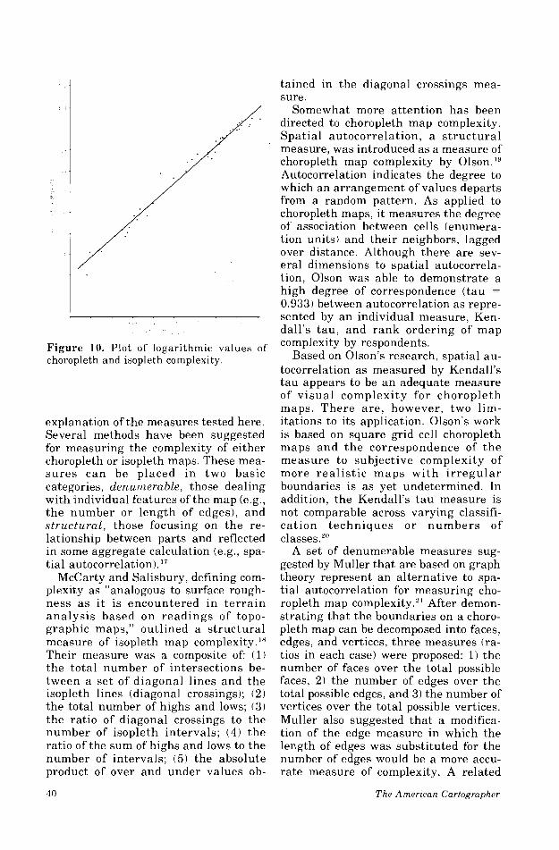
The visual appearance of the relation- ship of choropleth to isopleth map com- plexity suggests tha t a power function will provide a good fit. This function has the form X = aYb, with X and Y in this case being complexity values for isopleth and choropleth maps respectively, a, a constant reflecting the unit of measure- ment, and b, the exponent of the func- tion. This equation can be expressed logarithmically as logX = b (log Y) + log a. The advantage of employing the latter formula is tha t it is expressed graphi- cally as a straight line with log a as the y-intercept and b a s the slope of the line (Fig. lo) , and the values of log a and b can be found using ordinary regression. To determine the significance of the re- lationship, a correlation coefficient, r, was calculated for both the original val- ues and the logarithmic values, with re- sults of 0.964 and 0.987 respectively. (The line plotted on Fig. 10 represents the regression equation calculated for the logarithmic values and tha t in Fig. 9 represents t he curve defined by th is

I I I I L E T H I JEIPLLI l i

Figure 9. Plot of empirical choropleth ver- sus isopleth map complexity.

equation transformed back into a power function.)

OBJECTIVE MEASUREMENT OF COMPLEXITY

The analysis of subjective complexity of choropleth and isopleth maps has demonstrated a verv consistent relation- ship between the complexity of the maps using these two kinds of symbolization. This consistencv can now be used in de- veloping a physical measure of complex- ity tha t will be adaptable to both kinds of maps. If a physical measure of com- plexity can be shown to be an adequate approximation of the subjective com- plexity of either choropleth or isopleth maps, i t can be transformed to scale the complexity of the other kind of map a s well.

Review of Existing Measures

A brief review of previously suggested physical measures of map complexity is necessary to provide a background for an

Vol. 9, No. 1 , April 1982 39

Figure 10. Plot of logari thmic values of choropleth and isopleth complexity.

explanation of the measures tested here. Several methods have been suggested for measuring the complexity of either choropleth or isopleth maps. These mea- su re s can be placed in two basic categories, denumerable, those dealing with individual features of the map (e.g., the number or length of edges), and s tructural , those focusing on the re- lationship between parts and reflected in some aggregate calculation (e.g., spa- tial auto~orrelat ion) . '~

McCarty and Salisbury, defining com- plexity as "analogous to surface rough- ness a s i t is encountered in t e r r a in ana lys is based on readings of topo- graphic maps," outlined a s tructural measure of isopleth map complexity. Ix

Their measure was a composite of: (1) the total number of intersections be- tween a set of diagonal lines and the isopleth lines (diagonal crossings); (2) the total number of highs and lows; (3 ) the ratio of diagonal crossings to the number of isopleth intervals; (4 ) the ratio of the sum of highs and lows to the number of intervals; (5) the absolute product of over and under values ob-

tained in the diagonal crossings mea- sure.

Somewhat more attention has been directed to choropleth map complexity. S ~ a t i a l autocorrelation. a s t ruc tura l measure, was introduced a s a measure of choropleth map complexity by O l ~ o n . ' ~ Autocorrelation indicates the degree to - which an arrangement of values departs from a random pattern. As applied to choropleth maps, it measures the degree of association between cells (enumera- tion units) and their neighbors, lagged over distance. Although there are sev- eral dimensions to spatial autocorrela- tion, Olson was able to demonstrate a high degree of correspondence ( t au =

0.933) between autocorrelation a s repre- sented by an individual measure, Ken- dall's t au , and r ank ordering of map complexity by respondents.

Based on Olson's research, spatial au- tocorrelation as measured by enda all's tau appears to be a n adequate measure of v isua l complexity for choropleth maps. There a re , however, two lim- itations to its application. Olson's work is based on square grid cell choropleth maps and t h e correspondence of t he measure to subjective complexity of more rea l i s t ic maps wi th i r r egu la r boundaries is as yet undetermined. In addition. the Kendall's tau measure is not comparable across varying classifi- cat ion techniques o r numbers of classes."' ~~~

A set of denumerable measures sug- gested by Muller that are based on graph theory represent an alternative to spa- tial autocorrelation for measuring cho- ropleth map complexity." After demon- strating that the boundaries on a choro- pleth map can be decomposed into faces, edges, and vertices, three measures (ra- tios in each case) were proposed: 1) the number of faces over the total possible faces, 2) the number of edges over the total possible edges, and 3) the number of vertices over the total possible vertices. Muller also suggested tha t a modifica- tion of the edge measure in which the length of edges was substituted for the number of edges would be a more accu- rate measure of complexity. A related

The American Cartographer

measure, variation in region size, was proposed by Monmonier."

Lavin has compared measures of the various aspects of spatial autocorrela- tion (including the Kendall's tau mea- sure) with Muller's graph theoretic mea- sures.':' The comparison demonstrated a high level of redundancy among a l l measures tested. He concluded that any of these measures would be equally ef- fective in measuring complexity. Al- though graph theory measures have not been compared to subjective complexity, the i r apparent redundancy with the Kendall's tau measure of autocorrela- tion suggests tha t graph theory mea- sures will also prove to be highly related to the subjective complexity of choro- pleth maps. Graph theory measures also should not suffer from the major draw- back of the Kendall's tau autocorrela- tion measure: the lack of comparability across classification techniques and number of classes.

Due to their greater flexibility, then, and their ease of computation, the graph theoretic measures were selected for examination a s physical measures of map complexity. Graph theoretic mea- sures are suitable only to the measure- ment of choropleth map complexity. The approach taken, therefore, is to evaluate t he applicability of t he measures to choropleth maps and then, based on the re la t ionship demonst ra ted between subjective complexity of choropleth and isopleth maps, to assess the transforma- tion of the measures to the scaling of isopleth complexity.

Application of Graph Theory to Choropleth Map Complexity

In graph theory a graph is defined a s a collection of faces. edges. and vertices. A

2 - ,

choropleth base map can be considered a graph in which the faces, edges, and ver- tices a r e represented by map uni t s , boundaries between units, and the join- ing points of these boundaries. The base map used in the present study appears in Fig. 11 as such a graph. In this map there are 60 faces, 175 edges and 116 vertices. Assuming tha t edges between faces t h a t have equa l va lues a r e

EDGES FACE VERTEX

Figure 11. Graph transform of the base map.

omitted, the number of faces, edges, and vertices is a function of the size, shape, arrangement, and number of cells (Fig. 12). The more variation there is in the size of areas, the more edges and vertices will usually be required to make up a given number of units or faces. As the distribution of values mapped ranges from a homogeneous arrangement to a dispersed arrangement, the number of faces, edges, and vertices will all in- crease. Similarly, the less compact the units or the greater the number of units, the more faces, edges, and vertices there will be. The number of data classes also exhibi ts a pronounced effect on the number of faces, edges, and vertices; an increase in classes results in increased values of these variables (Fig. 13).

The number of faces, edges, and ver- tices seems to be related to the visual complexity of the map. Realizing this, Muller suggested t h a t rat ios of t h e number of faces, edges, and vertices on a map to the maximum possible numbers

Vol. 9, No. 1, April 1982

5 F,iceq

Original 11 i d - e a

7 ''crLLCeS

li- 9 vsccs Arrange-

men t 20 t . d i ~ 5

12 l ' e r t i c k s

Figure 12. Influence of variation in map units on the number of faces, edges. and vertices.

be used a s a measure of complexity." In the case of maps with four or more classes, it can be shown that it is possi- ble for every neighboring unit to belong

Figure 13. Influences of the number of class intervals on the number of faces, edges, and vertices.

to a different class and, therefore, the maximum values a r e equal to t he number of faces, edges, and vertices on the original map. On two- or three-class maps, however, the maximum possible number of faces (therefore edges and - vertices) will usually be less than the number of original units.

The deficiency of the graph theory measures as previously used is elimi- nated by simply using the total number of faces, edges, and vertices in the origi- nal base map, rather than the maximum possible number for any given choro- pleth map, a s the denominator in cal- culating the complexity ratios. The com- plexity measures for faces and vertices become:

observed number of faces Complex~ty, = -- --

number of o r~g ina l faces

observed number of vertices Complexity, = -

number of origlnal vertices

Neither the face nor the vertex mea- sure takes into account the size of faces. Simply dividing the observed number of edges by the total of original edges would have the same drawback. To par- tially account for face-size variation, Muller proposed using the number of original edges tha t fall between cat- egories on the map rather than the num- ber of observed edges." This measure results in a rough approximation of the length of edges, which tends to reflect face size. Although Muller expressed the opinion that a measure of actual edge length would result in an increase in-accuracv over edge number. a com- - parison of his results for the two mea- sures finds them redundant ( r = 0.96). Edge length is probably a significant improvement over the number of edges only in cases where there is a large vari- ation in length of the original edges. The complexity measure re la t ing to edges used in the present investigation therefore is:

number of o r~g ina l edges left Complexity, = .-

number of original edges

Each of the measures is calculated for the forty choropleth maps used in the complexity scaling procedure. If the

5 Faces

11 Edges

Figure 12. Influence of variation in map units on the number of faces, edges, and vertices.

be used a s a measure of complexity." In the case of maps wi th four or more classes, it can be shown that it is possi- ble for every neighboring unit to belong

Class 6 Vrrr lcc-s

Figure 13. Influences of the number of class intervals on the number of faces, edges, and vertices.

to a different class and, therefore, t he maximum values a r e equa l to t h e number of faces, edges, and vertices on the original map. On two- or three-class maps, however, the maximum possible number of faces (therefore edges and vertices) will usually be less than the number of original units.

The deficiency of the graph theory measures as previously used is elimi- nated by simply using the total number of faces, edges, and vertices in the origi- nal base map, rather than the maximum possible number for any given choro- pleth map, as the denominator in cal- culating the complexity ratios. The com- plexity measures for faces and vertices become:

observed number of faces Complexity, -

number of original faces

observed number of vertices Complexity, = -- . -

number of' original vertices

Neither the face nor the vertex mea- sure takes into account the size of faces. Simply dividing the observed number of edges by the total of original edges would have the same drawback. To par- tially account for face-size variation, Muller proposed using the number of original edges t h a t fall between cat- egories on the map rather than the num- ber of observed edges.'" This measure results in a rough approximation of the length of edges, which tends to reflect face size. Although Muller expressed the opinion tha t a measure of actual edge length would result in an increase in accuracy over edge number, a com- parison of his results for the two mea- sures finds them redundant ( r = 0.96). Edge length is probably a significant improvement over the number of edges only in cases where there is a large vari- ation in length of the original edges. The complexity measure re la t ing to edges used in the present investigation therefore is:

number of original edges left Complexity, = - --

number of original edges

Each of the measures is calculated for the forty choropleth maps used in the complexity scaling procedure. If t he

measures are accurate reflections of choropleth map complexity, a power function can be expected to provide the best description of the relationship be- tween the measures and subjective com- plexity. Linear regression of the log- arithms of subjective complexity with those of the objective complexity mea- sures is used as a means of evaluating - the correspondence of each measure with subjective complexity. The regres- sions result in correlation coefficients of 0.96, 0.97, and 0.98 for the face, vertex. and edge measures respectively. The logarithmic values and regression lines are plotted in Figs. 14-16. In contrast to Muller, but in agreement with Lavin, a high degree of redundancy is found among the three complexity measures ( r = 0.94 to 0.97)."' The high correlation values suggest that no significant im- provement in the explanation of vari- ance in subjective complexity would be achieved by a multivariate analysis.

Adaptation to Isopleth Map Complexity

Each of the three measures tested re- sults in an adequate approximation of the subjective complexity of choropleth maps. What remains, then, is to deter- mine the feasibility of adapting one of the measures to the scaling of isopleth

map complexity. Considering the simi- larity of results, the choice of a measure must be an arbitrary one. The edge mea- sure has the potential for accuracy over a larger range of maps due to its reflec- tion of face-size variation. and. there- fore, will be used here in attempting to relate a physical measure to the subjec- tive complexity of isopleth maps.

It has been demonstrated that subjec- tive complexity of choropleth maps is re- lated to the edge ratio measure accord- " ing to a power function. A power func- tion has also been shown to provide an explanation of the variation in subjec- tive complexity of choropleth and isopleth maps. Utilizing these functional rela- tionships, it is possible to transform the edge number measure to apply to isopleth map complexity. The correla- tion between the values predicted by this transformation with the values for subjective complexity of isopleth maps is used to evaluate the adequacy of this measure. A correlation coefficient of 0.976 is obtained. The edge number ratio appears to be a reasonable measure of both choropleth and isopleth map com- plexity, with its use for the latter being indirect.

Although the calculation for isopleth maps depends on information for choro- pleth maps, this limitation is not as se-

F A C E R A T I O

Figure 11. Relationship between complexity a n d the face rat io

1 .0 .

r - 0.97

0.9 b - 0.64

t a - 1 . 3 3 t- - 2 0.3 a E 0 U

, 0.7. > - + 0 W

2 0.6' 3 m

2 c l a s s o

3 c l a s s - r

4 c l a s s -0

5 c l a s s - a

0 . 3 1 0 , - 1 . 5 1 . 4 - 1 . 3 -1.2 - 1 . 1 - 1 . 0 - 0 . 9 -0.8 0 7 -0 6 -0.5 -0.4

V E R T E X R A T I O

Figure 15. Relationship between complexity and the vertex ratio.

vere as it may first appear. If the graph structure of the enumeration units is digitally encoded, the measure is quite simple to calculate. A computer algo- r i t hm can be used to determine the

1 I .

1 0-

0.9-

0 8 -

> t-

; 0.7- w

m

3 0 4 . ",

2 t- V

w 0 3 .

m 3 m

0 'l-

o 3 -

0 1 4 - 0 8 0 7 0 6 - 0 5 0 4 - 0 3 0 7 -01

EDGE RATIO

Figure 16. Relationship between complexity and the edge ratio.

edges of the original base map (graph) t ha t separate units in different cate- gories. From this number the edge num- ber ratio can be calculated without ac- tually having to produce a choropleth map. This feature would make it practi- cal to use the measure not only in situa- t ions in which comparison between choropleth and isopleth complexity is the objective, but a s a measure for the evaluation of individual isopleth maps as well.

Use of t he measure for choropleth maps is dependent on knowledge of the parameters of the power function relat- ing choropleth complexity to the edge number ratio. Application to isopleth maps is dependent on this knowledge a s well a s tha t of the parameters of the power function r e l a t ing isopleth to choropleth complexity. The particular functions obtained here are likely to be related, a t least in part, to the specific characteristics of the sample maps ex- amined. The relationship of choropleth complexity to the edge number ratio, a s well a s t ha t between choropleth and isopleth complexity, may vary with the number of enumeration units on the map or with different methods of class- ification tha t resul t in unequal num- bers of units in each class. General ap-

44 The Arnerlcan Cartographer

plication of the measure to all choro- pleth and isopleth maps will require examination of these questions.

As presented, the measure has two po- tential applications. One is to study the influence of map complexity on map ef- fectiveness. For a specific set of test maps, the parameters relating the edge numb,er ratio to choropleth and isopleth maps could be determined. It would then be possible\to derive a physical measure (the edge number ratio) of the complex- ity of each test map. The advantage here is that such a mqasure is well-defined and repeatable, thus allowing for com- parisons with other research findings.

An additional use is for situations in which a series of maps using the same base (e.g., a state) are to be produced. Once the parameters relating the edge number ratio to complexity of choropleth and isopleth maps were determined, complexity of any subsequently pro- duced maps could be measured without recourse to psychological scaling.

CONCLUSIONS A functional relationship has been

demonstrated between choropleth and isopleth map complexity with choropleth maps, a s expected, being judged more complex. A graph theory measure (the edge number ratio) appears to provide a n adequate measure of both choropleth and isopleth map complexity, although in the latter instance it is a n indirect measure. These resul t s provide the groundwork for examination of the re- lationship between communication ef- fectiveness and complexity of these two kinds of maps, since the relationship of one variable to another cannot be de- termined if no measure of the variable exists.

Several aspects of t he complexity- effectiveness relationship could be ad- dressed in future research. Most impor- tant perhaps is testing the hypothesis that map effectiveness decreases with increases in complexity. While this is probably true in a general sense, the re- lationship is not likely to be a simple linear one. Before it is possible to evalu- ate whether or not a map is too complex

for its intended purpose, this relation- ship must be understood. Because the complexity-effectiveness relationship may not be constant across symboliza- tion, a n examination of the relationship is necessary for each form of symboliza- tion considered. Although isopleth maps have been found to be visually less com- plex than choropleth maps, it does not necessarily follow tha t they are more ef- fective. Furthermore, we cannot ignore the fact that isopleth maps are based on the assumption of smoothness and con- tiguity of the distribution, and if tha t as- sumption is unreasonable a n isopleth map simply cannot be used. In addition to differences due to symbolization, i t may be found that the influence of com- plexity on map effectiveness varies with the situation in which the map is used or with different levels of training on the part of the map user.

The complexity measures tested here seem adequate for examining the impact of complexity on effectiveness. Many questions concerning map complexity, however, remain unanswered. One of the more obvious questions is how com- plexity of maps using symbolization other than choropleth or shaded isopleth compares with that of maps using these two methods. The relationship between complexity of choropleth maps and maps using other symbolization, such a s dots or perspective, should be considered. If the relationship is consistent, it may be possible to use, as a surrogate measure, the edge number ratio for choropleth maps with the appropriate transforma- tion. With no consistent relationship, an alternative measure designed specifi- cally for each form of' symbolization would be required.

An additional aspect of complexity t h a t deserves fu r the r a t ten t ion was brought to light with the creation of a complexity scale. Complexity appears to be the result of two somewhat indepen- dent factors: spatial variation of the mapped data and the number of classes into which data are divided. While the complexity measure developed he re combines the two factors, they could prove to have a n independent influence

Vol. 9, No. 1, April 1982

on map effectiveness. It may, therefore, be necessary to consider these hctors separately.

Because cartographers have greater control over the number of classes, it may be particularly important to con- sider this aspect of complexity sepa- rately. As the number of classes de- creases, map complexity decreases. At the same time, however, accuracy and perhaps visual and intellectual interest will d r o ~ . There mav be a lower limit of complexity below which its decrease is of no conseouence (or adverse consea uence ) to map effectiveness. One role ofthe car- tographer must be to reach for the op- timum in conlplexity rather than the least possible complexit,y.

The a u t h o r wishes to t h a n k Dr . J a m e s R Campbell tbr his comments on an earlier draft of this paper.

1. For the remainder of this paper, shaded i ~ p l e t h maps will be referred to simply a s isopleth maps.

2. The An~ericon College D~cllorzarj~, 1967. s.v. "Complex."

3. Broohv, David M., "Some Reflections on the . "

Complexity of Maps." Technical Papers. American Congrejs on Surveying and Mapping, 40th Annual Meeting, St . Louis, (March 19801, 345.

4. Morrison, Joel L.; "The Science of Cartogra- phy and Its Essential Processes." lntcrr~ntionnl Yearbook of Cartogrclphy, Vol. 16 I 1976). 84-97.

5. Muehrcke. Phillip C.: "The Influence of Spa- tial i\utocorrelation and Cross Correlation on Vi- sual Map Comparison." Proceedings, American Congress on Surveying and Mapping, 33rd Annual Meeting, Washington, D.C.. !March 1973), 321.

6. Olson. Judy M., "Autocorrelation as a Mea- sure uT Complexity," Proceedings, American Con- gress on Surveying and Mapping, (March 19721, 111 -119.

7. Muehrcke. Phi l l ip C , "Visual P a t t e r n Analysis: A Look a t Maps," unpublished Ph.D. Dissertation. University of Michigan (19691: Mor- rison, J. L., Method-Produced Error in Isarithnric Ma(l]~ing, American Congress on Surveying and Mapping, cartography Division, Technical Mono- graph. CA-5 t 1971).

8. J e n k ~ . G. and R. Coulr;on, "Class Intervals for Statistical Maps," Irtterttatior~al Yearbook of Cartography, Vol. 3 (19'741, 119-134.

9. S:~mpson, Robert J . , Surfircc II Graphics

System, Kansas Geological Survey, Lawrence, Kansas, 1975. (Computer program for contouring and manipulation of spatial da ta . )

10. Er~gen, T., "Psychophysics 11. Scaling Meth- ods," i n J. W. Kling and L. A. Riggs (eds.), Experi- nrental psycho log.^, Volun~e I ; Sertsulion a n d Per- ception, 3rd edition. Holt, Rinehart and Winston. Inc., New York (19721. 47-86.

11. Engen, 'r. and D. H. McBurney. "hfagnitude and Category Scales of t he Pleasantness of Odors," J o l ~ r n o l of Expcr~mental Psychology, 68 (19641. 435-440; Ekman, G., H. Eisler, and T. Kunnapas, "Brightness of Monocular Light as Measured by t h e Methods of Magni tude Production." Act0 Psychologica. 17 t 19601, 392-397; both loud~less and circle size are exarnined in Stevens, S. S . . Psychol~hvsrcs, G. Stevens (ed.1, John Wiley and Sons. New York (19751; grey tones are included in Stevens, S. S. and E. H. Galanter, "Ratio Scales a r ~ d Category Scales for a Dozen Perceptual Con- tinua." Jou r r~u l of Experin~erital Psychology. Vol. 54 (19571, 377-411; Stevens, S. S. and M. Guirao, "Subjective Scaling of Length and Area and the Matching of Length to Loudness and Brightness," J o u r n a l of E x p e r i r n ~ n t a i Psychology, Val. 6 6 I 19631, 1'77- 186.

12. Engen, 1972, op. cil. tftnt. 101. Galanter, E. , "Contemporary Psychophysics," in Neu, Directions in Psychology, Holt, Rinehwrt. and Winston, New York (19621, 153.

13. Engen, 1972. op. cit. iftnt. 101, 73. 14. Stevens, S. S. , "The D ~ r e c t Estimation of

Sensory Magnitudes-Loudness," Arr~criccln Jour- nal of Psychology, Vol. 69 (19561, 1 25.

15. Engen. 1972, op. cif. (f tnt . 101, 74. Stevens, 1975, op. r i t . (f tnt . 111.

16. Engen. 1972, op. cit. tftnt 10). 77. 17. Chipman, S. G.. "Complexity and Structure

in Visual Patterns." Journal of E.rprrirrietzta1 Psy- cholog,~, Vol. 106 (1977), 269-301.

18. hlccarty, H. H. and N. E. Salisbury, Visual Conrporisorl of Isopleth Maps cis a Meoris of Deter- ntinrng Cor-relations Between Sp(lt~(rlly Distributed Phenon~ena, State University of Iowa Studies in Geography, KO. 3, State University of Iowa, Iowa City (19611.

19. Olson. 1972, op. (.it. tftnt. 6). 20. Olson. 1972, op. cit. tftnt. 61. 21. Muller. J. C., "Mathemat~cal and Statistical

Comparisons in Choropleth Mapping," unpub- lished Ph.D. Dissertation, The University of Karl- sas, Lawrence, Kansas ( 1974).

22. Monmonier. Mark S., "Measures of Pattern Complexity for Choropleth hlaps," The Arrlerlcan Cnrtogropher, 1:2 (19741. 160.

23. Lavin, S., "Region Perception Variability in Choropleth Maps: Pattern Complexity Effects," unpublished Ph.D. Dissertation. The University of Kansas, Lawrence, Kansas (19791.

24. hfuller, 1974. op. cit. (f tnt . 21). 25. Ihid. 26. Muller, 1974, op. rif. (f tnt . 21); Lavin, 1979.

op. cit. tftnt. 231.

The A rnerican Cartographer-