MapInfo Professional and Vertical Mapper Exploring and ... · PDF fileMapInfo Professional and...

MapInfo Professional and Vertical Mapper Exploring and Working With Digital Elevation Models

Created By Kathryn Pierce

For MapInfo Professional and Vertical Mapper with Ela Dramowitz

February 22, 2007

Centre of Geographic Sciences


i

Table of Contents

Task 1: Finding Suitable Locations for Solar Plant in Lunenburg County, Nova Scotia........................................................................... 1

Clipping Study Area ............................................................................................................................................................................... 2

Polygons to Points, and Digital Elevation Model................................................................................................................................... 3

Method One ............................................................................................................................................................................................ 4

Method Two............................................................................................................................................................................................ 6

Task 2: Digital Elevation Model Analysis Techniques ............................................................................................................................ 10

Point Inspection .................................................................................................................................................................................... 11

Cross Section ........................................................................................................................................................................................ 12

Line Inspection...................................................................................................................................................................................... 13

Region Inspection ................................................................................................................................................................................. 14

Single Viewshed Analysis .................................................................................................................................................................... 15

Multiple Viewshed Analysis................................................................................................................................................................. 16

Complex Single Viewshed Analysis..................................................................................................................................................... 17

Generating Hillshade and Draping on 3-D View of Study Area .......................................................................................................... 18

Task 3: Interpolation Techniques ............................................................................................................................................................. 19

Triangulation With Smoothing ............................................................................................................................................................. 20

Nearest Neighbor without Overshoot ................................................................................................................................................... 21

Nearest Neighbor with Overshoot ........................................................................................................................................................ 22

Bilinear (Rectangular)........................................................................................................................................................................... 23

Inverse Distance Weighting.................................................................................................................................................................. 24

Kringing ................................................................................................................................................................................................ 25

Summary of Interpolation Methods Employed..................................................................................................................................... 27

Point Inspection for Various Interpolation Techniques ........................................................................................................................ 28


ii

Table of Figures

Figure 1, Clipped Study Area from Larger Lunenburg Dataset ................................................................................................................. 2

Figure 2, Polygons to Points in Vertical Mapper………………………………………………………………………………………….2

Figure 3, Digital Elevation Model (DEM).................................................................................................................................................. 3

Figure 4, Slope Grid and Aspect Grid ........................................................................................................................................................ 4

Figure 5, 2500 Meter Buffer ....................................................................................................................................................................... 4

Figure 6, Grid Query Results for Slope, Aspect, and Distance .................................................................................................................. 5

Figure 7, Appropriate Locations for Solar Power Plant ............................................................................................................................. 5

Figure 8, Reclassifications of Slope............................................................................................................................................................ 6

Figure 9, Reclassification of Aspect ........................................................................................................................................................... 6

Figure 10, Reclassifications of Distance Buffer ......................................................................................................................................... 7

Figure 11, Grid Calculator .......................................................................................................................................................................... 8

Figure 12, Weighted Sum and Weighted Sum Reclassification ................................................................................................................. 8

Figure 13, Data Flow Diagram for Method One......................................................................................................................................... 9

Figure 14, Data Flow Diagram Method Two.............................................................................................................................................. 9

Figure 15, Points and Point Inspection Table ........................................................................................................................................... 11

Figure 16, Line and Cross Section Graph................................................................................................................................................. 12

Figure 17, Line and Line Inspection Table............................................................................................................................................... 13

Figure 18, Polygons for Regional Inspection, and Region Inspcetion Table ........................................................................................... 14

Figure 19, Simple Single Viewshed Analysis........................................................................................................................................... 15

Figure 20, Simple Multiple Viewshed Analysis ....................................................................................................................................... 16

Figure 21, Complex Single Viewshed Analysis ....................................................................................................................................... 17

Figure 22, 3D View of Study Area ........................................................................................................................................................... 18

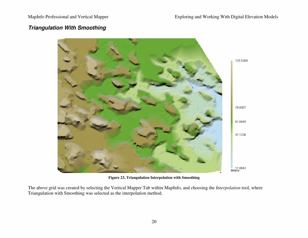
Figure 23, Triangulation Interpolation with Smoothing ........................................................................................................................... 20

Figure 24, Nearest Neighbor Interpolation without Overshoot ................................................................................................................ 21

Figure 25, Nearest Neighbor Interpolation with Overshoot ..................................................................................................................... 22

Figure 26, Bilinear (Rectangular) Interpolation........................................................................................................................................ 23

Figure 27, Inverse Distance Weighting Interpolation............................................................................................................................... 24

Figure 28, Interpolation using Kriging ..................................................................................................................................................... 25

Figure 29, Variogram for Kriging Interpolation ....................................................................................................................................... 26

Figure 30, Calculated Statistcs for Study Area......................................................................................................................................... 27


iii

List of Tables

Table 1, Summary of Interpolation Methods Employed .......................................................................................................................... 27

Table 2: Point Inspection for 10 Points, for all Interpolation Methods Employed in this Exercise ......................................................... 28


1

Task 1: Finding Suitable Locations for Solar Plant in Lunenburg County, Nova Scotia


2

Clipping Study Area

0

N

0

N

Figure 1, Clipped Study Area from Larger Lunenburg Dataset

The data area for this project is located in Lunenburg County, Nova Scotia. Files used included contours of the area and power lines.

The goal was to find the most appropriate area for a solar power plant, based on three criteria: aspect, slope, and distance. The best

aspect was considered to be between 112.5 degrees, and 247.5 degrees, with a slope greater than 10 degrees and a distance less than

2500 meters from power lines. The original data was clipped to a smaller area in MapInfo Professional, using a clip polygon, and then

removing all data outside of the selected area (figure 1). Two methods for finding suitable locations were applied: Method One,

involving querying the three parameters and then adding the three queries together, and Method Two, involved reclassification of the

slope, aspect and buffer, and then applying a weighting scheme to the three variables.


3

Polygons to Points, and Digital Elevation Model

Figure 2, Polygons to Points in Vertical Mapper Figure 3: Digital Elevation Model (DEM)

In order to extract the elevation and aspect data, and to create the digital elevation models of the area the contours and power lines

were converted to X and Y coordinates using the Polygon to Point Tool under the Vertical Mapper tab of MapInfo (figure 2).

Also done by selecting the Vertical Mapper tab within MapInfo, a Digital Elevation Model (DEM) was created for these coordinates

(figure 3).


4

Method One

Figure 4, Slope Grid and Aspect Grid

Figure 5, 2500 Meter Buffer

In the Grid Manager environment of Vertical

Mapper, under the Analysis Tab, the Create Slope

and Aspect tool was used to create the slope and

aspect maps for the study area (figure 4). A 2500

meter buffer was created around the power line

points by selecting Grid Buffer under the Vertical

Mapper Tab of MapInfo (figure 5).


5

Figure 6, Grid Query Results for Slope, Aspect, and Distance

Figure 7, Appropriate Locations for Solar Power Plant

In order to find the locations that were suitable for

the Solar Power Plant, a query needed to be

performed on the grids. As previously stated the

slope grid (figure 4) was queried to show slopes

that were greater than 10 degrees, the aspect grid

(figure 4) was queried to show aspects greater than

112.5 degrees, and less than 247.5 degrees, and the

buffer (figure 5) was queried to show less than

2500 meter distance (figure 6). These three queries

were then combined. The resulting areas thus met

all three criteria, and were therefore considered the

best locations for the solar power plant to be

located (figure 7).


6

Method Two

Figure 8, Reclassifications of Slope

Figure 9, Reclassification of Aspect

The slope, aspect and buffer grids used in Method One

were also used for method two. In this method the three

variables were reclassified, and then weighted, as

previously stated. All reclassifications were to have nine

intervals where 1 was the least suitable, and nine was the

most suitable. First slope, was reclassified to 9 intervals,

and then reclassified so that the categories were integers

from one to nine (figure 8). Next, aspect was reclassified,

where the suitability was determined by its orientation

(again between 122.5 degrees and 247.5 degrees) and

202.5 was the most suitable (figure 9).


7

Figure 10, Reclassifications of Distance Buffer

Distance, was reclassified to 9 intervals, and then reclassified so that the categories were integers from one to nine (figure 10).


8

Figure 11, Grid Calculator

Figure 12, Weighted Sum and Weighted Sum Reclassification

Finally the three reclassified grids were weighted. Slope

and distance were given a weighting of 0.3 and aspect,

considered most important in determining suitability, was

given a weighting of 0.4. The three grids were then

multiplied with their weights, and then all three were

added together with the Grid Calculator tool in Vertical

Mapper (figure 11). The final output was then reclassified

one final time into five intervals, where 5 were the most

suitable locations, and 1 the least suitable (figures 12).

Two data flow diagrams are also included demonstrating

Methods One and Two (figures 13 and 14).


9

Figure 13, Data Flow Diagram for Method One

Figure 14, Data Flow Diagram Method Two


10

Task 2: Digital Elevation Model Analysis Techniques


11

Point Inspection

Figure 15, Points and Point Inspection Table

Five points were created with MapInfo’s place marker tool (figure 15). These points were then saved as a new .TAB file. A point

inspection was preformed by selecting the Point Inspection tool under the Analysis tab of Vertical Mapper’s Grid Manager. The point

inspection was performed on all points, and the associated elevation for each point was extracted from the underlying grid, and the

point table was updated.


12

Cross Section

Figure 16, Line and Cross Section Graph

A line was drawn using the Line Tool in Mapinfo Professional, and saved as a .TAB file in order to create a cross section (figure 16).

By using the Cross Section tool, under the Analysis tab of the Grid Manager, Vertical Mapper was able to retrieve the elevations from

the underlying digital elevation model of the grid, and subsequently was able to create the cross section graph.


13

Line Inspection

Figure 17, Line and Line Inspection Table

Another line was drawn in MapInfo Professional and saved as a .TAB file, in order to perform a line inspection (figure 17). By using

the Line Inspection tool, from the Analysis tab of the Grid Manager, Vertical Mapper was able to update the table of the line from the

underlying grid to include information of the start, middle and end of the line, as well as the minimum, maximum, and mean of the

line’s elevations.


14

Region Inspection

Figure 18, Polygons for Regional Inspection, and Region Inspcetion Table

Two polygons were drawn on the grid, with MapInfo’s polygon tool, and saved as a new .TAB file, so that a region analysis could be

performed (figure 18). By selecting the Region Analysis tool, under the Analysis tab of the Grid Manager, Vertical Mapper extracted

minimum, maximum, and mean elevation’s within the polygons, and the number of cells that each contained and updated the table

associated with the two polygons.


15

Single Viewshed Analysis

Figure 19, Simple Single Viewshed Analysis

A place marker was placed on a place of high elevation of the study area in MapInfo, and saved as a .TAB file (figure 19). Simple

Viewshed Analysis was then performed on the single point, by selecting the Viewshed Analysis tool, under the Analysis tab of

Vertical Mapper’s Grid Manager and selecting the Simple parameter within the Viewshed Analysis Environment.. The resulting

analysis reflects the areas that are visible from the place marker.


16

Multiple Viewshed Analysis

Figure 20, Simple Multiple Viewshed Analysis

Five place markers were placed at various elevation in MapInfo, and saved as a .TAB file (figure 20). Simple viewshed analysis was

then performed on the single point by selecting the Viewshed Analysis tool, under the Analysis tab, as in the previous exercise. The

resulting analysis reflects the areas that are visible from the place markers to the other various place markers.


17

Complex Single Viewshed Analysis

Figure 21, Complex Single Viewshed Analysis

A complex single viewshed analysis was performed on the original place marker (figure 21). This was done by selecting the Viewshed

Analysis tool, under the Analysis tab of Vertical Mapper’s Grid Manager, and selecting the Complex parameter within the Viewshed

Analysis Environment. The resulting analysis reflects the areas that are visible from the place marker. Dark red values denote negative

values, which are below the selected place marker, and green values are above the selected place marker.


18

Generating Hillshade and Draping on 3-D View of Study Area

Figure 22, 3D View of Study Area

A hillshade drape file was created in Vertical Mapper, by selecting Make 3D Drape File, under the 3D View tab of Grid Manager. The

3D viewer was then created by selecting Run 3D Viewer, under the same 3D View tab. The resulting image reflects the elevations and

depressions of the study area in a 3D environment (figure 22).


19

Task 3: Interpolation Techniques

All grids created in this section will be derived from the original Polygons to Points (figure 2).


20

Triangulation With Smoothing

Figure 23, Triangulation Interpolation with Smoothing

The above grid was created by selecting the Vertical Mapper Tab within MapInfo, and choosing the Interpolation tool, where

Triangulation with Smoothing was selected as the interpolation method.


21

Nearest Neighbor without Overshoot

Figure 24, Nearest Neighbor Interpolation without Overshoot

The above grid was created by selecting the Vertical Mapper Tab within MapInfo, and choosing the Interpolation tool, where the

Nearest Neighbor technique was selected as the interpolation method. Within the Nearest Neighbor environment, the Without

Overshoot parameter was selected. This meant that while MapInfo was interpolating the elevations, it would not be allowed to

interpolate over or below the actual maximum and minimum elevation values of the study area, as shown in the Calculate Statistics

window (figure 23).


22

Nearest Neighbor with Overshoot

Figure 25 Nearest Neighbor Interpolation with Overshoot


Nearest Neighbor technique was selected as the interpolation method. Within the Nearest Neighbor environment, the With Overshoot

parameter was selected. This meant that while MapInfo was interpolating the elevations, it would be allowed to interpolate above or

below the actual maximum and minimum elevation values of the study area, as shown in the calculate statistics window (figure 23).


23

Bilinear (Rectangular)

Figure 26, Bilinear (Rectangular) Interpolation


Rectangular (Bilinear) technique was selected as the interpolation method.


24

Inverse Distance Weighting

Figure 27, Inverse Distance Weighting Interpolation

The above grid was created by selecting the Vertical Mapper Tab within MapInfo, and choosing the Interpolation, where the Inverse

Distance Weighting technique was selected as the interpolation method.


25

Kringing

Figure 28, Interpolation using Kriging

The above grid was created by selecting the Vertical Mapper Tab within MapInfo, and choosing the Interpolation, where the Kriging

technique was selected as the interpolation method.


26

Figure 29, Variogram for Kriging Interpolation

A variogram was created for the Kriging interpolation method. This graph show the actual variance and the predicted variance, or the

fitted model, shown as the white line on the graph.


27

Summary of Interpolation Methods Employed

Figure 30, Calculated Statistics of Study Area

Table 1, Summary of Interpolation Methods Employed

TriangulationWith Smoothing

Nearest NeighborWith Overshoot

Nearest NeighborWithout Overshoot

Bilinear(Rectangular)

Inverse Distance Weighting

Kriging

Surface Passes Through Original

Data Points

Allows Overshootand Undershoot

TriangulationInvolved

Z Min Z Max Comments

11.6711 125.5316

Weighted Moving Average

Weighted Moving Average

14.9989 122.0011

15 122

14.9989 122.4165

14.9989 122.0011

-5.5718 134.3717

The Z min and max are below and above the actual calculated statistics, because overshoot and undershoot are allowed as thetriangulation is being performed.

The Z min and max are below and above the actual calculated statistics, because overshoot and undershoot are allowed as thetriangulation is being performed.

The Z m in and m ax are just below and above the actual calculated statistics, because overshoot and undershoot aren’t allowed as thetr iangulation is being perform ed.

The Z m in and m ax are just below and above the actual calculated statistics, because overshoot and undershoot aren’t allowed.




28

Point Inspection for Various Interpolation Techniques

Table 2: Point Inspection for 10 Points, for all Interpolation Methods Employed in this Exercise

Through using the various interpolation techniques demonstrated in this assignment, it is apparent that different techniques give

various resulting elevations. Table Two is a point analysis, where ten points were created in MapInfo, and then analyzed, where values

represent the respective elevation of each point for each interpolation method. The variance between the different techniques deals

with the accuracy, and the allowance of overshoot and undershoot.

Date post:	06-Mar-2018
Category:	Documents
Upload:	dinhdang
View:	242 times
Download:	3 times

MapInfo Professional and Vertical Mapper Exploring and ... · PDF fileMapInfo Professional and...

Documents