Mapping and Modeling of Variable Source Areas in a Small ...

Mapping and Modeling of Variable Source Areas in a Small Agricultural Watershed

by

Kishorkumar Panjabi

A Thesis

presented to

The University of Guelph

In partial fulfillment of requirements

for the degree of

Doctor of Philosophy

in

Engineering

Guelph Ontario Canada

copy Kishorkumar Panjabi August 2015

ABSTRACT

MAPPING AND MODELING OF VARIABLE SOURCE AREAS IN A

SMALL AGRICULTURAL WATERSHED

Kishor Panjabi Advisor

University of Guelph 2015 Professor Ramesh Rudra

Modeling the spatiotemporal dynamics of Variable Source Areas (VSA) is challenging

since VSAs depend on a number of factors such as soil properties land use water

table topography geology and climatic conditions In spite of these challenges few

encouraging attempts have been made to develop models for quantification and

locating runoff generation areas based on VSA concepts However these

approaches need to be validated with field tests for their feasibility and accuracy

This research is divided into four main sections The first section discusses how an

advanced low cost remotely controlled digital Wireless Sensor Network (WSN)

system was developed to monitor and acquire climatic and hydrological data from a

distantly located watershed The developed WSN system was installed in a small

agricultural watershed near Elora Ontario and watershed observations of 45 rainfall

events from September 2011 to July 2013 were collected In the second section

significance of various climatic and hydrological factors affecting the spatiotemporal

variability of runoff generating areas are explored Analysis showed that the runoff

generating areas were strongly influenced by the seasons and that rainfall amoun

was the most dominant factor affecting these areas followed by initial soil moisture

and rainfall intensity

The third section includes modification of an existing distributed CN-VSA method by

incorporating seasonal variability of potential maximum soil moisture retention of the

watershed The simulations made with modified distributed CN-VSA predicted spatial

extent of saturated areas more accurately in ways consistent with VSA hydrology In

the fourth section an event based AGNPS model is reconceptualised based on VSA

hydrology concept by incorporating the Topographic Wetness Index (TWI) This

modeling approach demonstrates an easy method to predict the dynamics of VSAs

by combining VSA hydrology with existing SCS-CN runoff equation In this method

TWI was used in combination with land-use to define the CN values The simulated

results showed that in regions dominated by saturation excess runoff process

AGNPS-VSA model provides more realistic spatial distribution of runoff generating

areas than the AGNPS model based on traditional SCSndashCN method This research

will help to locate VSAs for applying targeted BMPs to control non-point source

pollution

iv

ACKNOWLEDGEMENTS

I am thankful to many people whose assistance was indispensable in the

completion of my research Firstly I want to thank my advisor Dr Ramesh Rudra for

accepting me as his student his wonderful guidance thoroughness and promptness

in reviewing my work Without his patience constructive comments and feedback it

would have been impossible for me to handle research work of this kind I would also

like to extend my sincere gratitude to my committee members Dr Bahram

Gharabaghi Dr Gary Parkin and Dr Pradeep Goel for their participation in my

dissertation committee and their valued guidance Lastly I am greatly indebted to Dr

W Trevor Dickinson for his technical assistance and expert advice

I want to thank Dr D Joy Dr Omar Ahmed and Dr KG Singh for their

technical support and enriching ideas on my study I am also grateful to Adam

Bonnycastle for helping me on GIS whenever I was clueless I am deeply

appreciative of Eric Kassab Michael Haines Francois Poilly Bhavin Kapadia Aws

Nabeel Jacob Chol Andrew Eldebs Xiao Cong Li Paritosh Roy Sarvapreet Kaur

and Sabrina Fraser for being extremely helpful with the field and laboratory studies I

am also grateful to the faculty research scientists office staff and fellow graduate

students of the School of Engineering for always lending me a hand when needed

I would like to say special thanks to my wife Savita and my daughters Rutu

and Rhea for supporting my endeavours Finally many friends who have helped me

stay sane during my stay at grad school I greatly value their friendship and I deeply

appreciate their belief in me

v

Table of Contents

CHAPTER 1 1

Introduction 1

11 Runoff generation mechanisms 1

12 Variable source areas 2

13 VSAs related to water quality 4

14 Variable Source Area modeling 5

15 Problem statement 7

16 Research objectives 10

17 Expected outcome impacts and benefits 11

18 Thesis organization 11

19 References 13

CHAPTER 2 19

Variable Source Area Hydrology Past Present and Future 19

21 Introduction 19

22 Historical overview 22

23 Factors affecting Variable Source Areas 28

24 Dynamics of Variable Source Areas 31

25 Monitoring of Variable Source Areas 32

251 Active methods of monitoring 32

252 Passive methods of monitoring 34

26 Modeling Variable Source Areas 35

27 Present status 38

28 Towards future developments 40

29 Concluding Remarks 44

210 References 46

211 Transition to Chapter 3 60

CHAPTER 3 61

Development and field evaluation of a low cost wireless sensor network

system for hydrological monitoring of a small agricultural watershed 61

31 Introduction 61

vi

32 Design and development of WSN 65

321 Modification of WSN system (Phase 3) 68

3211 Sensors 68

3212 Power supply 69

3213 Sturdiness of node assembly 69

3214 Communication connectivity 70

3215 Data visualization tool for WSN 71

33 Laboratory calibration of nodes 72

34 Field testing of WSN 74

35 Field data collection 77

36 Summary and conclusions 82

37 References 83


CHAPTER 4 87

Field investigation of the runoff generating areas in a small agricultural

watershed in southern Ontario 87

41 Introduction 88

42 Materials and Methods 90

421 Study area 90

422 Monitoring the climatic and hydrologic variables 91

423 Analysis procedure 94

43 Results and Discussion 95

431 Factors affecting the variability of runoff generating area 101

4311 Effect of rainfall amount 101

4312 Effect of initial soil moisture content 102

4313 Effect of rainfall intensity 104

4314 Effect of five-day antecedent rainfall amount 105

4315 Effect of rainfall duration 106

432 Multivariable Linear Regression analysis 109

433 Relation of minimum contributing areas with basin and storm index 111

434 Description of spatial and seasonal minimum runoff generating areas 114

44 Conclusions 118

vii

45 References 119


CHAPTER 5 122

Development and evaluation of modified distributed CN-VSA method for

estimation of spatial distribution of Variable Source Areas 122

51 Introduction 123

52 Description of distributed CNndashVSA method 126

521 Predicting the saturated fractional area of watershed 127

522 Spatial location of the Runoff Generating Areas 129

53 Material and Methods 131

531 Description of Watershed 131

532 Distributed CN-VSA method 133

533 Application of Distributed CN-VSA method 136

534 Modified distributed CN-VSA method 138

535 Application of the Modified Distributed CN-VSA method 139


541 Comparison of runoff amounts estimated byboth the methods 140

542 Spatial distribution of runoff 145

55 Conclusions 148

56 References 149


CHAPTER 6 154

Incorporation of Variable Source Area Runoff Generation Mechanism into

the Hydrology of the AGNPS Model 154

61 Introduction 154

62 The AGNPS model 158

63 The CN method and its application to VSA concept 161

64 Incorporation of Variable Source Area concept into AGNPS model 163

65 Study area 166

66 Input data 167

67 Calibration of AGNPS and AGNPS-VSA models 169

viii

68 Discussion of Results 170

681 Comparative evaluation of AGNPS-VSA and AGNPS approaches 171

682 Comparative evaluation between AGNPS-VSA and AGNPS model 174

69 Conclusions 179

610 References 179

CHAPTER 7 184

Conclusions and recommendations 184

71 Conclusions 184

72 Recommendations for future research 185

Apendices 187

Appendix - A 187

Appendix - B 191

Appendix - C 194

Appendix - D 199

Appendix - E 203

ix

Table of Figures

Figure 11 Flow chart showing organization of thesis 12

Figure 31 Typical distributed wireless sensor network system 64

Figure 32 Components of the developed WSN system 70

Figure 33 Calibration diagram of soil moisture sensor 73

Figure 34 Calibration diagram of pressure sensor 74

Figure 35 WSN and manual readings of soil sensor on September 12 2011 75

Figure 36 WSN and manual readings of pressure sensor on September 12 2011 75

Figure 37 WSN and manual readings of soil sensor on December 27 2011 76

Figure 38 WSN and manual readings of pressure sensor on December 27 2011 76

Figure 39 Layout of the study watershed at Elora Ontario 77

Figure 310 Field observations of rainfall and runoff event dated June 01 2012 80

Figure 311 Field observations during September 2012 81

Figure 312 Field observations during year 2012 81

Figure 41 Layout of study watershed and sub-watersheds in ERS 90

Figure 42 Monitoring locations of soil moisture sensors and V-notch weirs 92

Figure 43 Relationship between MRGA and rainfall amount 101

Figure 44 Relationship between MRGA and initial soil moisture 103

Figure 45 Relationship between MRGA and maximum rainfall intensity 104

Figure 46 Relationship between MRGA and five-day antecedent rainfall 106

Figure 47 Relationship between MRGA and rainfall duration 107

Figure 48 Relationship between MRGA and basin moisture index 112

Figure 49 Relationship between MRGA and storm index 114

Figure 51 Layout of the study watershed in Elora Research Centre Elora 132

Figure 52 Topographic Wetness Index map of study watershed 133

Figure 53 Distributed CN-VSA method-Step 1 134



Figure 56 Distributed CN-VSA method-Step 4 (rainfall event on 28-May-2013) 136

Figure 57 Application of the distributed CNndashVSA method (nine rainfall events) 137

Figure 58 Application of the modified distributed CNndashVSA (nine rainfall events) 139

x

Figure 59 Comparison of the runoff simulated by the distributed CNndashVSA

method with the observed runoff 143

Figure 510 Comparison of the runoff simulated by the modified distributed

CNndashVSA method with the observed runoff 144

Figure 511 Comparison of spatial distribution of runoff estimated by distributed

CNndash VSA method and modified distributed CNndashVSA method (spring) 146


CNndashVSA method and Modified distributed CNndashVSA method (summer) 147


CNndash VSA method and Modified distributed CNndashVSA method (fall) 148


Figure 62 Topographic Wetness Index class map of the study watershed 169

Figure 63 Comparison of the runoff simulated by the AGNPS-VSA model

with the observed runoff for the calibration phase 171


with the observed runoff for the validation phase 172

Figure 65 Comparison of the runoff simulated by the AGNPS model with the

observed runoff for the calibration phase 172


observed runoff for the validation phase 173

Figure 67 Spatial pattern of runoff generating areas simulated by AGNPS-VSA

model for spring summer and fall rainfall events 177

Figure A1 Precipitation temperature and soil moisture data of fall 2011 189

Figure A2 Precipitation temperature and soil moisture data of year 2012 189


Figure A4 Map showing locations of soil testing in study watershed 191

Figure A5 Soil textural triangle (USDA) 192

Figure A6 LiDar data acquiring instrument (Leica Geo systems Cndash10) 195

Figure A7 Lidar generated DEM of study watershed 196

Figure A8 Cross Section profile at X-X of study watershed 196

Figure A9 Cross Section profile at Y-Y of study watershed 197

Figure A10 Topographic slope and contours of the study watershed 197

Figure A11 Drainage lines and field outlet of study watershed 198

xi

Figure A12 Flow chart showing development of Topographic Index 200

Figure A13 Topographic Wetness Index map of study watershed 202

Figure A14 Runoff hydrograph on dated 03-May-12 204

Figure A15 Spatial distribution of runoff coefficient of event dated 03-May-12 204

Figure A16 Runoff hydrograph on dated 26-July-12 205

Figure A17 Spatial distribution of runoff coefficient of event dated 26-July-12 206

Figure A18 Runoff hydrograph on dated 02-Dec-12 207

Figure A19 Spatial distribution of runoff coefficient of event dated 02-Dec-12 207

xii

List of Tables

Table 41 Characteristics of field soil 91

Table 42 Main characteristics of 45 observed rainfall-runoff events 96

Table 43 Summary statistics of 45 observed rainfall-runoff events 98

Table 44 Seasonal statistics of minimum runoff generating area 99

Table 45 Summary of correlation of various factors with MRGA 108

Table 46 Statistical correlation of various factors with MRGA 108

Table 47 Simulated multivariable regression equations and their statistics 110

Table 48 Simulated multivariable regression equation for Tp and their statistics 111

Table 49 Summary of climatic and hydrological data of a spring event helliphelliphelliphellip115

Table 410 Summary of climatic and hydrological data of a summer event 116

Table 411 Summary of climatic and hydrological data of a fall event 117

Table 51 Comparison of the runoff simulated by both the methods 141

Table 61 Parameters of AGNPS-VSA and AGNPS models for Fall season 170

Table 62 Comparison of the runoff by AGNPS and AGNPS-VSA model 174

Table A1 Monthly temperatures of ERS during 2011 2012 and 2013 187

Table A2 Monthly Precipitation of ERS during 2011 2012 and 2013 188

Table A3 Percentages of the primary soil separates (0-20 cm) 192

Table A4 Soil testing results of bulk density and Ks 193

Table A5 Summary of climatic and hydrological characteristics of a spring event 203

Table A6 Summary of climatic and hydrological characteristics of summer event 205

Table A7 Summary of climatic and hydrological characteristics of a fall event 206

xiii

List of abbreviations

ADC Analog to Digital Converter

Af Fractional area

AGNPS Agricultural Non-Point Source Pollution Model

AWC Antecedent wetness condition

BMP Best Management Practices

C Runoff coefficient

CN Curve Number

CREAMS Chemicals Runoff and Erosion from Agricultural Management

Systems model

CSA Critical Source Area

D Duration of Rainfall

d Depth

DEM Digital Elevation Model

E Coefficient of efficiency (Nash-Sutcliffe)

EI Erosion Index

EPIC Erosion-Productivity Impact Calculator model ERS Elora Research Station

GIS Geographic Information System

GP Guelph Permeameter

GRASS Geographic Resources Analysis Support System

GWLF General Watershed Loading Function model

HAA Hydrologically Active Area

HSA Hydrologically Sensitive Area

I Rainfall intensity

Ia Initial abstraction

IO Input Output

IMC Initial moisture content

Ks Saturated hydrologic conductivity

L Length

Lidar Light Detection And Ranging

m rank of position

MFD Multiple Flow Direction

MHz Mega Hertz

MOE Ministry of the Environment

MVLR Multi Variable Linear Regression

n Number of samples

NDVI Normalized Difference Vegetation Index

NIR Near infra-red

xiv

NPS Nonpoint source pollution

NRCS Natural Resources Conservation Service

NWRI National Water Research Institute

Q Runoff

ON Ontario

p Probability

P Rainfall amount

Pe Effective precipitation

PCB Printed circuit board

r Product-moment correlation coefficient

R2 Coefficient of Determination

RGA Runoff generating area

RL Reduced level

RMSE Root-mean-squared error

S Potential maximum retention

SAS Statistical Analysis System

SCS-CN Soil Conservation Service curve number

SFD Single Flow Direction

SI Storm index

SMDR Soil Moisture Distribution and Routing model

SAR Synthetic-aperture radar

SMoRMod Soil Moisture-based Runoff Model

SWAT Soil amp Water Assessment Tool

SWAT-VSA VSA-based Soil and Water Assessment Tool

SWAT-WB Water Balance-based Soil and Water Assessment Tool

tanβ Local gradient

TDR Time-domain reflectometry

TI Topographic Index

TIN Triangular Irregular Network

Tp Time of ponding

TOPMODEL Rainfall-runoff model based on topography

TRCA Toronto Regional Conservation Authority

TVA Tennessee Valley Authority

TWI Topographic Wetness Index

USDA United States Department of Agriculture

US EPA United States Environmental Protection Agency

VSA Variable Source Area

VSAS1 VSA Simulator model 1

VSLF Variable Source Loading Function model

WSN Wireless Sensor Network

1

CHAPTER 1

INTRODUCTION

11 Runoff generation mechanisms

Surface runoff due to excess rainfall andor snowmelt constitutes an important part of

the water cycle and a dominant pathway of nonpoint source pollution Therefore

identifying the location of high runoff generating areas is very important for the

application of best management practices (Hoover 1990 Leh et al 2008 Singh and

Woolhiser 2002)

The location of runoff generating areas (RGAs) in a landscape depends on the runoff

generating mechanism Infiltration excess and saturation excess are the two primary

hydrological mechanisms of runoff generation Infiltration excess is also called

Hortonian overland flow and occurs when the application of water to the soil surface

exceeds the infiltration capacity of the soil (Horton 1933 1940) The infiltration rate

depends on soil properties land use and landscape conditions (Hewlett and Hibbert

1963 Hornbeck and Reinhart 1964 Whipkey 1965) Infiltration excess runoff

depends on magnitude of the rainfall intensity and often low rainfall intensity does not

generate any runoff With some exceptions the infiltration excess is often assumed to

take place uniformly over the landscape under arid and semi-arid conditions

In contrast saturation excess runoff occurs when soil becomes saturated from below

as the water table rises to the land surface either from excess rainfall or from lateral

subsurface flow Precipitation over these saturated areas results in runoff (Dunne and

2

Leopold 1978) The portions of the landscape generating saturation excess runoff

varies seasonally as well as within a storm thus they are generally termed as

variable source areas (VSA) or hydrologically active areas (Frankenberger et al

1999 Walter et al 2000) Saturation excess runoff generally occurs in humid and

thickly vegetated regions with permeable shallow soils underlain by an impervious

layer (Dunne and Black 1970 Merwin et al 1994)

In watersheds both infiltration excess and saturation excess runoff generating

mechanisms may contribute to overland flow however often only one of the

processes dominates (Betson 1964 Dickinson et al1970) The infiltration excess

approach can be useful at a field scale but may not be good enough to simulate

hydrologic processes at a watershed scale Consequently appropriate spatial and

temporal representation of infiltration excess and saturation excess runoff in a

watershed is the most significant task in hydrological modeling studies (Mehta et al

2003 2004)

12 Variable source areas

Variable Source Area (VSA) hydrology is a watershed runoff process where runoff

during the precipitation event is generated on saturated surface areas of the

landscape In other words precipitation on saturated areas becomes ldquosaturation

excessrdquo overland flow Runoff from these areas is generated by saturation excess

after the water table rises and saturates the landscape

The expansion and contraction of VSAs during and following a storm are generally

influenced by the subsurface flow Once the top layer of soil becomes saturated

3

continuation of rainfall increases the interflow delivering water to the base of slopes

and near stream areas resulting in expansion of the runoff generating areas After

the cessation of rainfall reduced downstream moisture movement results in the

contraction of VSAs (Loganathan et al 1989)

In the VSA hydrology runoff generating areas are not uniformly distributed over the

landscape but is concentrated in specific saturated areas (Garen et al 2005) Many

researchers have suggested that relatively small portions of a watershed contribute to

direct runoff whereas remaining regions rarely generate runoff (Arteaga et al 1973

Betson 1964 Moldenhauer et al 1960) VSAs generally develop along the lower

portions of hillslopes topographically converging or concave areas valley floors

shallow water table areas and adjoining the streams (Amerman 1965)

VSAs contributing to overland flow are very active sensitive and dynamic in nature

and may vary significantly spatially and temporarily within the storm or seasonally As

an extension of the saturation excess process VSAs within a watershed develop

within hours or days and expand or contract depending on the landscape wetness

and rainfall amount (Dunne and Black 1970 Hewlett and Nutter 1970 Walter et al

2000) The spatial and temporal variability of VSAs depend upon the rainfall amount

rainfall intensity landscape wetness soil characteristics land use topography water

table depth and its geographical location (Sivapalan et al 1987)

Field research has concluded that VSAs often originate from small but identifiable or

at least interpretable fractions of a watershed and produce most of the watershed

runoff (Gburek and Sharpley 1998 Srinivasan et al 2000) Dickinson et al (1970)

4

observed that the variable source areas in the Blue Springs Creek watershed (ON)

having sub-humid continental climate ranged from 1 to 21 of the watershed

area Jordan (1994) reported that about 10 to 20 of the catchment generate

saturation excess runoff while the remaining areas infiltrate and does not contribute to

any runoff

13 VSAs related to water quality

Contamination of freshwater is a chronic problem worldwide that has serious

consequences on ecosystem and human health Nonpoint source (NPS) pollution

from agriculture ldquois the leading source of water quality impacts in rivers and lakes the

second largest source of impairments to wetlands and a major contributor to

contamination of estuaries and groundwaterrdquo (US EPA 2005)

The development of large amounts of storm runoff in a watershed has many

implications on the environment and surface water contamination (Gregor and

Johnson 1980) In watersheds dominated by saturation excess runoff generating

mechanism some fractional areas are more susceptible of generating surface runoff

than others

Walter et al (2000) suggested that VSAs are associated with enhanced hydrologic

sensitivity compared to other non-runoff generating areas and hence are called as

Hydrologically Sensitive Areas (HSAs) Runoff from HSAs poses the risk of quickly

delivering potential pollutants to surface water bodies When these areas intersect

with land use that can possibly contribute pollutants they are termed Critical Source

Areas (CSAs) (Gburek et al 2002) The CSAs constitute a comparatively small area

5

of the watershed but are responsible for contributing a large fraction of pollution

loads to the surface waters (Sen et al 2008)

Agricultural runoff is responsible for polluting rivers and lakes as well as impairing

wetlands Pollutants resulting from farming activities include sediment fertilizers

pesticides pathogens metals and salts (Miller et al 1982) Farming activities result

in contamination and degradation of the environment and pose the greatest threat to

the worldrsquos drinking water supplies Hydrologically runoff from agricultural areas

primarily originates from HSAs rather than from the entire watershed therefore the

studies dealing with agricultural pollution of surface waters need to be cognizant of

the role of VSA hydrology (Govindaraju 1996 Qiu 2003 2010)

In recent times protection of local drinking water sources is a major environmental

challenge (Davidson et al 2005) Protecting sources of water and taking the

necessary measures to restore water quality is vital for human aquatic and

ecosystem health Therefore identification of VSAs is crucial for application of BMPs

for managing a wide range of water quality problems and reducing the loads of

sediment nutrients and bacteria to streams lakes and reservoirs

14 Variable Source Area modeling

Modeling spatial and temporal variability of VSA is very challenging since the

development of a VSA depends on multiple factors such as soil properties water

table depth topography land use geology climatic conditions and topographic

position in the landscape In spite of difficulties and challenges few encouraging

6

attempts have been made to develop models for quantification and locating runoff

generation areas based on VSA concepts

During the last two decades the increase in computational power advancement in

Geographic Information System (GIS) and widespread availability of digital

geographic data have led to the development of complex distributed deterministic

models A number of models such as TOPMODEL (Beven and Kirkby 1979) DHSVM

(Wigmosta et al 1994) SMDR (Steenhuis and Molen 1986) SMoRMod (Zollweg et

al1996) have some capability to include variable source area concepts These

models having variable degree of complexity are based on distributed moisture

accounting within the segments of a watershed are rarely used because they require

copious calibration and large amount of input data (Pradhan et al 2010)

Recently there have been some re-conceptualizations of widely-used water quality

models to account for VSA hydrology The Soil and Water Assessment Tool (SWAT)

and the Generalized Watershed Loading Function (GWLF) have both been

successfully re-conceptualized to integrate VSA hydrology in SWAT-VSA (Easton et

al 2008) and Variable Source Loading Function (VSLF) (Schneiderman et al 2007)

However these models are validated largely on long-term average simulations and

not by rigorous field tests Moreover these models are somewhat more complicated

and computationally intensive than most engineering applications warrant (Mills

2008)

In a new attempt a modified version of SWAT called Water Balance-Based Soil and

Water Assessment Tool (SWAT-WB) has been developed (White 2009) SWAT-WB

7

uses a physically-based soil water balance technique to model surface runoff instead

of using the traditional Soil Conservation Service curve number (SCS-CN) method

(USDA-SCS 1972) However this approach needs to be tested with observed field

data for its feasibility and accuracy of mapping VSAs in a watershed

The majority of present water quality protection strategies assessment methods and

best management practices are based on conventional infiltration excess runoff

concept and water quality management approaches still rely on popular water quality

models based on infiltration excess runoff generating mechanism since these are

well established and user-friendly with their proven nutrient transport and soil erosion

sub routines However for the areas dominated by saturated excess runoff

mechanism these models may not be able to predict the correct locations of runoff

generating areas (Chapi 2009 Pradhan 2010) At present VSA hydrology is not

usually used for water quality protection (Qui et al 2007) hence there is a need to

develop new approaches for monitoring and modeling to identify critical management

areas from VSAs

15 Problem statement

Field observations and repeated field mapping during and after rainfall events can be

effectively used for mapping the size magnitude location and variability of runoff

generating areas Runoff generating areas during and after storm events can easily

be observed and identified as VSAs by monitoring the watershed because these

areas are wetter than other areas and need more time to dry after a storm event (Qiu

2003)

8

The traditional analog type hydrological monitoring systems lack resolution and

scalability In addition cabling requirements in the field restricts the spatial size of the

monitoring area (Oliveria et al 2011) Rapid development in digital technology

wireless communication and low power micro sensing technologies has made

Wireless Sensor Networks (WSNs) economically feasible to use in hydrologic

research (Song et al 2008) Unlike other networks WSNs are designed for specific

applications in hydrology (Verma 2013) During last few decades substantial

advancements have been made in the field of WSNrsquos technology but the

development of WSNs for hydrological and environmental research is still in the

relatively primitive stages During the last decade a number of research studies have

focused on the field of WSN technology for environmental monitoring but very few of

them are supported by actual field evaluation (Szewczyk et al 2004) At present no

simple or low cost off-the-shelf solution exists for hydrological monitoring applications

Hence there is a need to develop a low cost efficient and remotely operated WSN

system for monitoring climatic and hydrologic variables in a watershed

VSA hydrology has been universally acknowledged as a basic principle of

hydrological science since 1970 but it has been noted that the quantitative

understanding of the VSA concept is far from complete and its application to

hydrologic calculations is not fully developed Another poorly understood process is

saturation overland flow Further very limited field data is available to physically verify

or support the various theories of VSA hydrology and its governing factors There is

still ambiguity among the scientific community about the dominating factors affecting

the development and variability of the VSAs Therefore there is a need for field

9

research to investigate the significance of various factors responsible for

spatiotemporal variability of runoff generating areas in a watershed

Many studies have shown that the theoretical basis of the SCS-CN method is valid for

both Hortonian and saturation excess runoff generating mechanisms (Hjelmfelt 1980

Steenhuis et al 1995) However the majority of current water quality models use CN-

values computed on the basis of soil infiltration capacity and land use to estimate

storm runoff (Walter and Shaw 2005) These models implicitly presume that the runoff

is generated by Hortonian runoff mechanism and hence fail to account for the effects

of topography and moisture distribution which are very important factors in the

watersheds dominated by saturation excess runoff generating mechanism

(Schneiderman et al 2007 Srinivasan et al 2002)

The Distributed CNndashVSA method developed by Lyon et al (2004) is one of the

promising newer methods that incorporates VSA concept to simulate the aerial

distribution of saturation excess runoff This physically-based method uses a

traditional SCS-CN approach to predict runoff volume and spatial extent of saturated

areas and distributes runoff source areas within the watershed using a Topographic

Wetness Index (TWI) approach This simple method can be easily integrated with

existing hydrological models for predicting the locations of runoff generating areas

based on VSA concept However it needs to be validated with observed field data to

ensure its feasibility and accuracy of mapping the VSAs in a watershed

It is an established fact that a very high percentage of nonpoint source pollution loads

from rural agricultural watersheds are generated by few intense rainfall events due to

10

high amount of generated runoff (McBroom et al 2003) The rainfall events are also

the main contributor in establishing hydrological connectivity between agricultural

land and streams and transporting NPS pollution loads (Kim et al 2006) Hence

there is a need to develop a distributed event based model based on VSA hydrologic

concept to simulate overland flow and accurately identify runoff generating areas

within a watershed Such a model would aid in the identification quantification and

modeling of runoff generation mechanisms and runoff generating areas that are vital

for best management practices applications in agricultural watersheds Moreover

these models would help to develop strategies to minimize pollutant loads in surface

waters by accurately predicting the locations of runoff generating areas

16 Research objectives

The overall objective of this study is to investigate the spatial and temporal variability

of the variable source areas in small agricultural watershed in the climatic conditions

of Ontario The specific objectives of this research are

1) To develop a low cost robust and remotely operated WSN system for

monitoring and collecting climatic and hydrological data from a distantly

located agricultural watershed

2) To investigate the significance of factors affecting the spatial and

temporal variability of runoff generating areas in a watershed by field

experimentation and to identify VSAs

11

3) To evaluate and improve the performance of an existing variable source

area modeling approach (distributed CN-VSA) for mapping the variable

source areas in a watershed with field observed data

4) To develop and evaluate the performance of an event based distributed

hydrological model for simulation of the dynamics of variable source

area

17 Expected outcome impacts and benefits

The outcome of this research would provide a methodology to map sources of

surface runoff in a fieldwatershed The result of this comprehensive monitoring and

modeling study on VSA hydrology concept would help in locating hot spots of runoff

generation Mapping of such source areas would result in selection of specific and

targeted best management practices for the development of economically efficient

and environmentally sustainable water quality and NPS pollution management

strategies In addition for areas where monitoring is not possible the developed VSA

modeling approach will allow to understand the hydrological behavior of headwater

areas of a watershed the process of soil erosion and sediment transport Therefore

this is a major step towards development and implementation of best management

practices (BMPs) on potential pollution generating areas in a watershed to reduce the

loads of sediment nutrients pollutants and bacteria to streams lakes and reservoirs

18 Thesis organization

This thesis is organized into seven chapters as shown in Fig 14 Chapters two

three four five and six are written as separate papers in a journal article format

12

These individual papers describe different aspects of the research and include an

introduction methodology results discussion and conclusion

Figure 11 Flow chart showing organization of thesis

The thesis begins with Chapter 1 which includes introduction of the topic problem

statement objectives and expected outcome

Chapter 1 Introduction

Chapter 2 Literature review

Chapter 3 Development of Wireless Sensor Network System

Chapter 4 Field monitoring data collection and analysis

Chapter 5 Development of Modified

CN-VSA method

Chapter 6 Development of

AGNPS-VSA model

Chapter 7 Conclusions and

Recommendations

Appendices

13

Chapter 2 includes a literature review of past research an explanation of the present

situation and an outline of the future of variable source area hydrology including the

use of emerging technologies for delineating and modeling VSAs

Chapter 3 discusses the development and field evaluation of a low cost WSN system

for hydrological monitoring in a small agricultural watershed

Chapter 4 describes the field monitoring data collection and statistical analysis of

rainfall and runoff data from a study watershed

Chapter 5 includes development and evaluation of the modified distributed CN-VSA

approach for predicting VSAs of runoff generation

Chapter 6 is devoted to development and evaluation of an event-based distributed

model for modeling and mapping variable source areas in a watershed

Chapter 7 wraps up the thesis by describing the conclusions and future

recommendations pertaining to this research Lastly details of the study watershed

and climatic and hydrological characteristics of three randomly selected rainfall-runoff

events are included in the appendices

19 References

Amerman C R (1965) The use of unit-source watershed data for runoff prediction

Water Resources Research 1 499-507

Arteaga F E Rantz S E (1973) Application of the source-area concept of storm

runoff to a small Arizona watershed Journal of Research US Geological

Survey 1(4) 493-498

Betson R P (1964) What is watershed runoff Journal of Geophysical Research

69 1541-1552

14

Borah D K Bera M (2003) Watershed-Scale Hydrologic and Nonpoint-Source

Pollution Models Review of mathematical bases Transactions of the ASAE

46(6) 1553-1566

Chapi K (2009) ldquoMonitoring and modeling of runoff generating areas in a small

agricultural watershedrdquo PhD Thesis Guelph University of Guelph

Davidson A Howard G Stevens M Callan P Fewtrell L Deere D Bartram J

(2005) Water Safety Plans Managing Drinking-Water quality from catchment to

consumer Geneva Italy WHO

Dickinson W T Whiteley H (1970) Watershed areas contributing to runoff

International Association of Scientific Hydrology Bulletin 96 12-26

Dunne T Leopold L B (1978) Water in Environmental Planning NY W H

Freeman and Co pp 818

Dunne T Black R D (1970) An experimental investigation of runoff production in

permeable soils Water Resources Research 6 478-490

Easton Z M Daniel R F Walter M T Cowan DM Schneiderman E M

Steenhuis T S (2008) Re-conceptualizing the soil and water assessment tool

(SWAT) model to predict runoff from variable source areas Journal of

Hydrology 348 279ndash 291

Frankenberger J R Brooks E S Walter M T Walter M F Steenhuis T S

(1999) A GIS-Based Variable Source Area Hydrology Model Hydrological

Processes 13 805-822

Garen D C Moore D S (2005) Curve number hydrology in water quality

modeling Uses abuses and future directions) Journal of the American Water

Resources Association 41(2) 377-388

Gburek W J Sharpley A N (1998) Hydrologic controls on phosphorus loss from

upland agricultural watersheds Journal of Environmental Quality 27 267ndash277

Govindaraju RS (1996) Modeling overland flow contamination by chemicals mixed

in shallow soil horizons under variable source area hydrology Water Resources

Research 32 doi 10102995WR03639 issn 0043-1397

Gregor DJ MG Johnson RC Loeher CS Martin W Rast (1980) Nonpoint

source phosphorus inputs to the Great Lakes Phosphorus management

strategies for lakes Ann Arbor Science Publishers 37-60

15

Hewlett J D Hibbert A R (1963) Moisture and energy conditions within a sloping

soil mass during drainage Journal of Geophysical Research 68(4) 1081-1087

Hewlett J D Nutter W L (1970) The varying source area of streamflow from

upland basins Paper presented at Symposium on Interdisciplinary Aspects of

Watershed Management Montana State University Bozeman New York

American Society of Civil Engineers 65-83

Hjelmfelt AT (1980) Curve number procedure as infiltration method Journal of

Hydrology 106 1107ndash1111

Hornbeck JW Reinhart K G (1964) Water quality and soil erosion as affected by

logging in steep terrain Journal of Water conservation 19 23-27

Horton R E (1933) The role of infiltration in the hydrologic cycle Transactions of

the American Geophysical Union 14 446-460

Horton R E (1940) An approach toward a physical interpretation of infiltration

capacity Proceedings of the Soil Science Society of America 5 399-417

Hoover J R (1990) Seep and runoff detector design and performance to determine

the extent and duration of seeprunoff zones from precipitation on a hillside

Transactions of the American Society of Agricultural Engineers 33 1843-1850

Jordan J P (1994) Spatial and temporal variability of storm flow generation

processes on a Swiss catchment Journal of Hydrology 153 357-382

Kim J S Oh SY Oh KY (2006) Nutrient runoff from a Korean rice paddy

watershed during multiple storm events in the growing season Journal of


Leh M D Chaubey I Murdoch J Brahana J V Haggard B E (2008)

Delineating runoff processes and critical runoff source areas in a pasture

hillslope of the Ozark Highlands Hydrological Processes 22 4190ndash4204

Loganathan G V Shrestha SP Dillaha TA Ross BB (1989) Variable Source

Area Concept for Identifying Critical Runoff-Generating Areas in a Watershed

Virginia Water Resources Research Center

Lyon S W Walter M T Gerard-Marchant P Steenhuis T (2004) Using a

topographic index to distribute variable source area runoff predicted with the

SCS curve number equation Hydrological Processes 18 2757-2771

McBroom M Beasley R S Chang M Gowin B Ice G (2003) ldquoRunoff and

sediment losses from annual and unusual storm events from the Alto

16

experimental watersheds Texas 23 years after silvicultural treatmentsrdquo The

first interagency conference on research in the watersheds Benson AZ

Matthew W McBroom 607ndash613

Mehta V K Steenhuis T S Johnson B Mark S Coon W F Boll E S (2003)

Application of Two Hydrologic Models with Different Runoff Mechanisms to a

Hillslope Dominated Watershed in the Northeastern US A Comparison of

HSPF and SMR Journal of Hydrology 284 57-76

Mehta V K Walter M T Brooks E S Steenhuis T S Walter M F Johnson

M Boll J Thongs D (2004) Application of SMR to modeling watersheds in

the Catskill Mountains Environmental Modeling amp Assessment 9(2) 77-89

Merwin I A Stiles W C Vanes H M (1994) Orchard groundwater management

impacts on soil physical properties Journal of the American Society of

Horticultural Sciences 119(2) 216-222

Miller MH Robinson JB Coote DR Spires AC Wraper DW (2002)

Agriculture and water quality in the Canadian Great Lakes Basin III

Phosphorus Journal of Environment Quality 11(3) 487-493

Mills J (2008) ldquoTesting a Method for Predicting Variable Source Areas of Runoff

Generationrdquo Cornell University Ithaca NY Master of Engineering Report

Department of Biological and Environmental Engineering

Moldenhauer WC Barrows WC Swartzendruber D (1960) Influence of rain

storm characteristics on infiltration measurements Transactions of the

International Congress on Soil Science 7 426-432

Oliveira L M Rodrigues J J (2011) Wireless sensor networks a survey on

environmental monitoring Journal of communications 6(2) 143-151

Pradhan NR Ogden F L (2010) Development of a one-parameter variable source

area runoff model for ungauged basins Advances in Water Resources 33

572ndash584

Qiu Z (2003) A VSA-Based Strategy for Placing Conservation Buffers in Agricultural

Watersheds Environmental Management 32(3) 299-311

Qiu Z (2010) Variable source pollution Turning science into action to manage and

protect critical source areas in landscapes Journal of Soil and Water

Conservation 65(6) 137A-141A

Schneiderman E M Steenhuis T S Thongs D J Easton Z M Zion M S

Neal A L Mendoza G F Walter M T (2007) Incorporating variable source

17

area hydrology into a curve-number-based watershed model Hydrological


Sen S Srivastava P Dane J H Yoo K H Shaw J N (2008) Spatial-Temporal

variability and hydrologic connectivity of runoff generation areas at Sand

Mountain region of Alabama Providence Rhode Island ASABE Annual

International Meeting June 29 ndash July 2 2008

Singh V P Woolhiser D A (2002) Mathematical modeling of watershed

hydrology Journal of Hydrologic Engineering 7(4) 270-292

Sivapalan M Beven K Wood E F (1987) On hydrologic similarity 2 A scaled

model of storm runoff production Water Resources Research 23(12) 2266-

2278

Song J Han S Mok A K Chen D Lucas M Nixon M (2008) Wireless HART

Applying wireless technology in real-time industrial process control Real-Time

Embedded Technology and Applications Symposium IEEE RTAS08 377-386

Srinivasan M S Wittman M A Hamlett J M and Gburek W J (2000) Surface

and subsurface sensors to record variable runoff generation areas Transactions

of the ASAE 43(3) 651-660

Srinivasan M S Gburek W J Hamlett J M (2002) Dynamics of storm flow

generation A hillslope-scale field study East-central Pennsylvania USA

Hydrological Processes 16 649-665

Steenhuis T S Muck R E (1988) Preferred movement of non-adsorbed

chemicals on wet shallow sloping soils Journal of Environmental Quality

17(3) 376-384

Szewczyk R Osterweil E Polastre J Hamilton M Mainwaring A Estrin D

(2004) Habitat monitoring with sensor networks Communications of the ACM

47(6) 34-40

US Environmental Protection Agency (EPA) (March 2005) EPA 841-F-05-001

Agricultural Nonpoint Source Fact Sheet

Verma R (2013) A Survey on Wireless Sensor Network Applications Design

Influencing Factors amp Types of Sensor Network International Journal of

Innovative Technology and Exploring Engineering 3(5) 2278-3075

Walter MT Shaw SB (2005) Discussion lsquoCurve number hydrology in water

quality modeling Uses abuses and future directionsrsquo by Garen and Moore

Journal of American Water Resources Association 41(6)1491ndash1492

18

Walter M T Walter M F Brooks E S Steenhuis T S Boll J Weiler K

(2000) Hydrologically sensitive areas Variable source area hydrology

implications for water quality risk assessment Journal of soil and water

conservation 3 277-284

Whipkey R Z (1965) Subsurface storm flow from forested slopes Hydrological

Sciences Journal 10(2) 74-85

White ED (2009) Development and application of a physically based landscape

water balance in the swat model Cornell University USA Master of Science Thesis

19

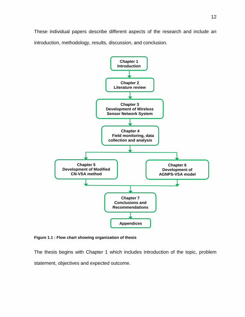
CHAPTER 2

Variable Source Area Hydrology Past Present and Future

Abstract

Variable Source Area hydrology is a watershed runoff process where surface runoff

generates on saturated surface areas In other words the rain that falls on saturated

areas results in ldquosaturation excessrdquo overland flow Variable source areas develop

when a soil profile becomes saturated from below after the water table rises to the

land surface either from excess rainfall or from shallow lateral subsurface flow This

paper presents a review of the past and present research developments in the field of

variable source area hydrology Existing methods and approaches for monitoring

delineating and modeling the VSAs are presented Further the advances in remote

sensing technology higher resolution satellites and aerial photography for

delineating saturated areas are discussed for the future of monitoring and modeling

variable source areas

Keywords Variable source area Hydrological modeling SCS Curve Number

Topographic index Nonpoint Source Pollution

21 Introduction

The concept of Variable Source Area (VSA) was first developed by the US Forest

Service (1961) but the term variable source area is credited to Hewlett and Hibbert

(1967) Dunne and Black (1970) and Hewlett and Nutter (1970) are also known to be

20

foundational contributors to the VSA hydrology concept During the 1960s and 1970s

intensive field experiments in small catchments were conducted to map the spatial

patterns of runoff generating areas and their seasonal variations These studies

supported the VSA concept and since then many efforts have been made to explain

and predict the spatial patterns of VSAs (Barling et al 1994 Beven and Kirkby 1979

Sivapalan et al 1987)

VSAs develop when a soil profile becomes saturated from below after the water table

rises to the land surface This can happen due to either excess rainfall or shallow

lateral subsurface flow from upslope catchment areas (Dunne and Black 1970 Dunne

and Leopold 1978 Beven 2001 Srinivasan et al 2002 Needelman et al 2004)

However this is contrary to the long standing Hortonian theory which assumes that

runoff takes place when the rainfall intensity exceeds the infiltration capacity of the

soil (Horton 1933) Hortonian overland flow does not happen at low rainfall intensities

and is often assumed to take place uniformly over the landscape However many

studies have shown that the fraction of the watershed susceptible to saturation

excess runoff varies seasonally and within the rainfall event thus these runoff

generating areas are generally termed as VSAs or hydrologically active areas

(Frankenberger et al 1999 Walter et al 2000)

VSAs are generally influenced by the rainfall amount and shallow lateral subsurface

flow Their spatial and temporal variability are different depending upon the rainfall

amount depth of the water table antecedent wetness condition soil characteristics

landscape topography and the geographical location of the area (Sivapalan et al

1987) VSAs commonly develop along the lower portions of hillslopes topographically

21

converging or concave areas valley floors shallow water table areas and adjoining

the streams (Amerman 1965)

Over the years a number of physically-based distributed models based on VSA

hydrology concept have been developed (Knapp 1974 Kirkby et al 1975 Beven and

Kirkby 1979 Frankenberger et al 1999 Takeuchi et al 1999 Ogden and Watts

2000) However the requirement of a large amount of input data and the necessity of

copious calibration often restricts practical application of these models in ungauged

basins (Pradhan et al 2010) During the last decade few re-conceptualizations of

widely-used hydrological models have been developed to include the VSA hydrology

However these process-based models are also computationally intensive and

complicated for engineering applications and need to be validated or supported by

rigorous field tests (Mills 2008 Chapi 2009)

Even though the concept of VSA hydrology has become popular during the last two

decades it is not usually used in water quality protection procedures due to the lack

of user-friendly watershed models based on VSA hydrological processes (Qiu et al

2007) The majority of current water quality protection procedures assessment

methods and Best Management Practices (BMPs) are based on conventional

infiltration excess runoff theory (Walter et al 2000) Water quality managers still rely

on the water quality models to establish the sources and fates of nonpoint source

pollutant fluxes because they are well documented and user-friendly with proven

nutrient transport and soil erosion transport components (Wellen et al 2014) These

models primarily assume infiltration excess as the principal runoff producing

mechanism and fail to correctly locate the runoff generating areas as the dominant

22

factors affecting the infiltration excess runoff generation mechanism are different than

the factors that control saturation excess process (Schneiderman et al 2007)

Advancements in digital technology wireless communication and embedded micro

sensing technologies have created a good potential for hydrological and

environmental monitoring (Poret 2009) Recent developments in the field of Wireless

Sensors Network (WSN) and communication systems have further revolutionized the

field of hydrological monitoring These are substantial improvements over traditional

monitoring systems and are promising new technologies for studying hydrological

responses of watershed headwaters in order to model the spatial-temporal variability

of VSAs (Trubilowicz et al 2009) Moreover increasingly available computational

power and new innovations in remote sensing higher resolution satellites and aerial

photography are promising future technologies for monitoring and for paving the way

for formulating standard modeling methods for identification and quantification of

VSAs (Pizurica et al 2000)

The main objectives of this study are to (1) provide an overview of the past and

present research related to developments of VSA hydrology (2) describe present

methods and approaches for monitoring delineating and modeling the VSAs and (3)

discuss the monitoring and modeling of VSAs in the light of advancements in digital

technology remote sensing higher resolution satellites and aerial photography

22 Historical overview

The earlier concept of overland flow was that storm runoff is primarily the result of

overland flow generated by an excess of rainfall that exceeds the infiltration capacity

23

of the soil The infiltration excess runoff known as Hortonian flow (Horton 1933 1937

1940) occurs when the application of water to the soil surface exceeds the rate at

which water can infiltrate into the soil The infiltration rate depends on soil type land

use vegetation and landscape wetness (Hewlett and Hibbert 1963 Hornbeck and

Reinhart 1964 Whipkey 1965) Infiltration excess runoff does not happen at low

intensities and is often assumed to take place uniformly over the landscape Pilgrim

et al (1978) Jordan (1994) Perrin et al (2001) Wetzel (2003) and Godsey et al

(2004) reported that the variability of soils in a watershed may allow both infiltration

excess and saturation excess runoff generating mechanisms simultaneously in humid

areas However Scherrer et al (2007) observed that one or more of these

mechanisms often dominate depending on the characteristics of watershed such as

vegetation slope soil clay content and antecedent soil moisture condition

Horton (1943) recognized that surface runoff rarely occurs on soils well protected by

forest cover due to ldquosomewhat unusual conditionsrdquo The term ldquounusual conditionrdquo can

be seen as the first concept on VSAs in a watershed Subsequently Hoover and

Hursh (1943) and Hursh (1944) described a ldquodynamic form of subsurface flowrdquo

contributing to storm flow generation in forested areas Subsequently Roessel (1950)

emphasized the importance of subsurface flow and groundwater contributions to

streamside outflow Cappus (1960) based on the study in a watershed dominated by

sandy soils provided clear field evidence of subsurface storm flow within the context

of the VSA concept He divided the watershed into ldquorunoff areasrdquo and ldquoinfiltration

areasrdquo The runoff generating areas were completely water-saturated terrains while

in the infiltration areas the saturated hydraulic conductivity of soils was so high that

24

the rain falling onto these areas was absorbed and no runoff was generated

(Ambroise 2004)

Hursh and Fletcher (1942) discovered that subsurface flows and groundwater

depletion can also contribute to stream flow in humid regions This was further

confirmed by Hewlett and Hibbert (1963) Reinhart et al (1963) and Whipkey (1965)

Many researchers contributed the VSA concept between 1961 and 1975 but Hewlett

had the honor of describing the significance of the VSA concept (Jackson 2005)

The Tennessee Valley Authority (TVA) (TVA 1964 1965) investigated eight rainfall

events in two gauged watersheds and found that runoff is first generated from the low

lands while slopes and ridges gradually contribute as soil moisture increases during

the storm TVA called these areas ldquopartial watershed areasrdquo and ldquodynamic watershed

conceptrdquo Zavodchikov (1965) referred to these areas as ldquoeffective areasrdquo In a study

conducted on an agricultural research watershed Amerman (1965) concluded that

runoff generating areas are randomly distributed on ridge tops valley slopes and

valley bottoms

Betson (1964) proposed the partial area concept suggesting that only certain fixed

regions of a watershed contribute to runoff whereas remaining regions rarely

generate runoff The partial areas result from variability in infiltration rate and intensity

of rainfall in time and space that generate Hortonian overland flow The main

difference between VSA and the partial area concept is that variable source areas are

produced by saturation excess runoff as a result of the soils inability to transmit

25

interflow further downslope and expand and contract spatially and temporally

whereas partial areas in a watershed remain spatially static (Freeze 1974)

The paper by Hewlett and Hibbertrsquos (1967) lsquoFactors affecting the response of small

watersheds to precipitation in humid areasrsquo is a benchmark research in the field of

VSA hydrology Their research proved to be a well-accepted alternative to the

previous concept of Hortonian overland flow Later on Kirkby and Chorley (1967)

introduced slope concavities and areas with thinner surface soil as locations where

surface saturation may occur leading to the development of VSAs Based on the field

investigations and analysis of a number of rainfall events Ragan (1967) revealed that

a small fractional area of a watershed contributed significant flow to the storm

hydrograph Similarly Arteaga and Rantz (1973) analyzed eleven rainfall events also

reported that only certain areas in a watershed contribute runoff while the remaining

areas did not contribute

Hewlett (1969) carried out experiments on mountainous watersheds of the southern

Appalachians within the Coweeta hydrologic laboratory This area consists of steep

slopes highly infiltrative surface soils small valley aquifers pathways and turnover

rates of water in forested or well-vegetated environments He concluded that the

interflow and VSA runoff were the main drivers of storm flow with interflow delivering

water to the base of slopes and temporary expansion and contraction of the VSAs

around the stream channel (Dunne 1970 Dunne and Black 1970 Troendle 1985

Loganathan et al 1989)

26

Whipkey (1969) measured the outflow from various horizons of a forest soil and found

that the first layer of the soil was the main source of runoff due to its saturation by a

perched water table over an impeding layer This was further validated by Betson and

Mariusrsquos (1969) studies on the runoff generation mechanism and observations that a

shallow A horizon of the soil was frequently saturated From this observation they

concluded that a thin A horizon of the soil is a primary source of runoff and this soil

layer causes a heterogeneous runoff generation pattern within the watershed

Dunne and Black (1970a1970b) used the water table information to define the

saturated areas in a forested watershed to investigate the saturation excess runoff

generation process From this study they concluded that a major portion of the storm

runoff was generated by small parts of the watershed saturated by subsurface flow

and direct precipitation They also indicated that the top soil profile becomes

saturated due to a rise in the water table and rainfall over these wet areas results in

saturated excess overland flow This type of saturated areas generally develops in

valley floors and close to the streams

Pearce (1976) observed that both the Hortonian runoff and saturation excess runoff

generation mechanisms occur concurrently in humid forest areas and a small part of

the watershed produces runoff Later Freeze (1980) supported this theory and

Mosley (1979) also drew similar conclusion after monitoring a small forest watershed

with steep (35deg) slopes and shallow (average 055 m) soils on impermeable strata

Mosley (1979) observed that only 3 of net precipitation became overland flow while

the subsurface flow was dominant during rainfall events and quick flows indicating the

importance of saturated excess mechanisms for stream flow generation Steenhuis

27

and Muck (1988) also observed that the rainfall intensities rarely exceed the

infiltration capacity of shallow hillside soils and these observations were later

supported by Merwin et al (1994)

Many studies have shown that VSAs often occur across the small but predictable

fractional areas of a watershed (Srinivasan et al 2000 2002) Gburek (1990 1998)

described the VSAs as areas consisting of the stream surface and the area of surface

saturation caused by the groundwater table intersection within the land surface above

the elevation of a stream

Walter et al (2000) suggested the concept of Hydrologically Active Areas (HAAs)

They observed that in the VSA hydrology dominant watersheds some areas are

more prone of generating runoff for all rainfall events These areas are also named as

hydrologically sensitive areas (HSAs) when connected to the primary surface bodies

of water Hydrologically sensitive areas coinciding with potential pollutant loading

areas are defined as Critical Source Areas (CSAs) or referred as Critical

Management Zones (Gburek et al 2002)

Joel et al (2002) indicated that the Hortonrsquos concept of runoff generation does not

provide an adequate description of hydrological processes at the hillslope level He

observed that on average the larger plots of 50 m2 area generate more runoff per

unit areas than smaller plots (025 m2) and supported the observations of Chorley

(1980) that the Hortonrsquos theory becomes less accurate with increase in catchment

size

28

Srinivasan et al (2000) Hernandez et al (2003) and McGuire et al (2007) observed

that the interaction between static characteristics (topography soil land cover) and

dynamic characteristics (time varying rainfall characteristics soil moisture conditions

hydraulic conductivity of soil and depth to the water table) affects variability of VSAs

Latron and Gallart (2007 2008) suggested that the VSAs can be classified into two

categories according to the process of soil saturation The VSAs developed due to

the rising of the water table to the surface was termed as A type VSAs and the areas

with top upper layer saturated due to the perched water table were classified as B

type VSAs

Lastly Buda et al (2009) demonstrated the influence of subsurface soil properties on

surface runoff generation in agricultural watersheds with VSA hydrology which could

be useful for improving the accuracy of existing VSA prediction models

23 Factors affecting Variable Source Areas

Knowledge of the factors affecting the development and variability of VSAs is critical

for developing a better understanding of the response of a watershed to rainfall

event The main factors affecting the spatial and temporal variability of VSAs are

watershed characteristics topography water table depth soil type land use rainfall

characteristics surface and groundwater hydrology geology and climatic conditions

(Walter et al 2000)

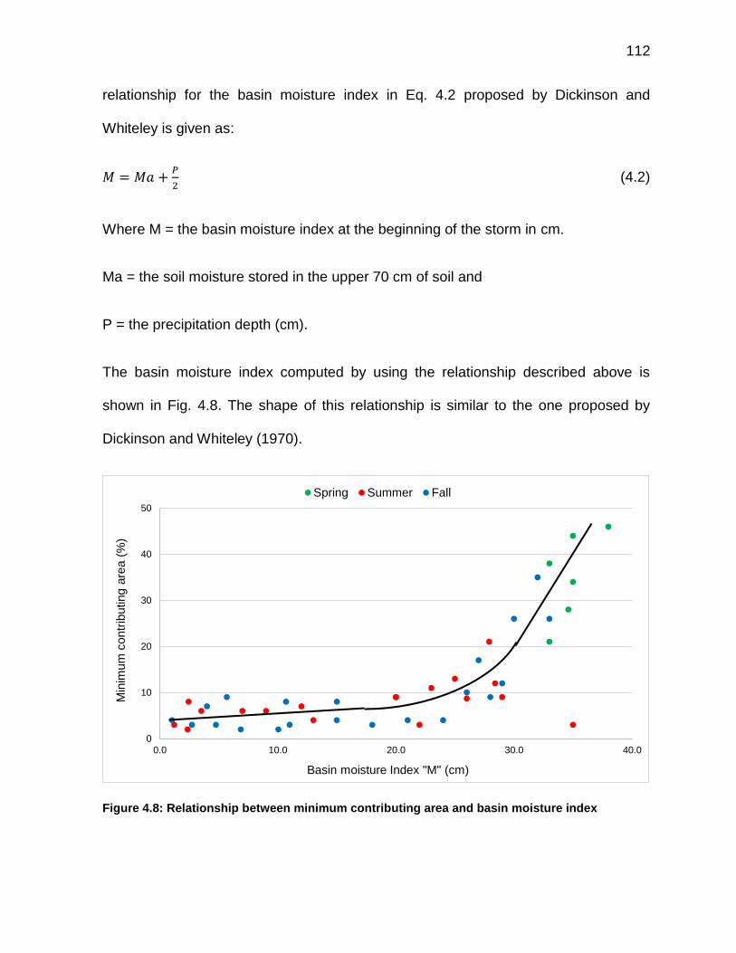
Dickinson and Whiteley (1970) were the first to evaluate VSAs and concluded that the

most important factors affecting VSAs were stream surface area pre-event soil

moisture rainfall intensity and depletion of soil moisture storage as the storm

29

progresses Moore et al (1976) indicated that topography soil type vegetation and

antecedent moisture index are key factors affecting the saturated areas in small

watersheds Lee and Delleur (1976) concluded that the drainage basin slope and

roughness of landscape are the controlling factors of the VSAs Dunne and Leopold

(1978) emphasised the importance of storm size phreatic zone and the subsurface

flow system for runoff generation Beven (1978) suggested that soil type topography

and basin size play an important role in the hydrological response of headwaters

Beven and Wood (1983) concluded that the storm rainfall initial moisture deficit and

geomorphologic structure of the watershed are critical factors affecting the variability

of VSAs Hernandez et al (2003) reported that hill sides with concave and low relief

areas are more susceptible and create large VSAs compared to steep slope hillsides

Pearce et al (1986) reported antecedent wetness physical properties of soil water

table depth and storm magnitude are the most important factors in seasonal

expansion and contraction of VSAs Kwaad (1991) analyzed summer and winter

runoff generation mechanisms and observed that summer runoff follows the Horton

model of runoff generation process and is controlled by the rainfall intensity whereas

winter runoff follows the saturated excess mechanism and is affected by the amount

of rainfall rather than the rainfall intensity Verhoest et al (1998) suggested the need

for soil moisture properties groundwater seepage and topography to map the spatial

variability of variable source areas Troch et al (2000) explained that the

development of VSAs in a watershed depends on land relief and wetness of the

landscape Elsenbeer and Vertessy (2000) reported that the hydrological response of

30

a watershed can be controlled by lithological properties of soils and their interactions

with rainfall characteristics

Kirkby et al (2002) examined the effects of several factors on surface runoff

generation using a Variable Bucket Model and concluded that the slope storm size

and storm duration are the important factors affecting the runoff generation Gupta

(2002) reported that saturated hydraulic conductivity bulk density of soil elevation

and field slope are dominant factors affecting runoff generation during the summer

months Hernandez et al (2003) suggested that topography soil hydraulic properties

and depth of the water table show good correlation with the variability of VSAs

Nachabe (2006) related soil type topography rainfall vegetation cover and depth of

the water table to the expansion and contraction of VSAs Gomi et al (2008)

observed that the delivery of surface runoff from hill slopes to stream channels

depends upon the timing and size of rainfall events surface vegetation and soil

conditions

Literature review indicates that the development and variability of VSAs depends on

many factors however depending upon the objective many researchers have

considered different factors as primordial for mapping variable source areas at

different scales (Kirkby et al 2002 Leh et al 2008) Despite substantial research

conducted during the last five decades there is still knowledge to be gained

concerning the main factors affecting development and variability of variable source

areas

31

24 Dynamics of Variable Source Areas

The VSAs contributing to surface runoff are very dynamic in nature and significantly

vary spatially and temporarily within a storm as well as seasonally VSAs within the

watershed expand or shrink depending on subsurface flow landscape wetness and

rainfall amount (Hewlett and Nutter 1970 Dunne and Black 1970 Walter et al 2000)

Riddle (1969) summarized the magnitude of variable source areas in a watershed

from the literature suggested that the distributions of the runoff generating area were

very similar despite the variable characteristics of the basins The majority of stream

flow producing event were generated by less than 10 of the watershed areas

Dickinson and Whiteley (1970) studied twenty three rainfall events between the

months of October and November and found that VSAs in the watersheds ranged

between 1 to 21 They also indicated that the VSAs were relatively small at the

beginning of the storm depending on stream surface area and soil moisture near the

streams Moreover they observed that the minimum contributing areas ranged from 0

to 59 with a mean of 20 and a median value of 10

Freeze (19721974) revealed after experimenting in the Reynolds Creek Watershed

near Boise (Idaho) that storm flow originates from 1 to 3 of the landscape and

generally does not exceed 10 of the watershed area A field survey during spring

season by Shibatani (1988) showed that the extent of the saturated surface near a

stream zone ranged from 8 of the total watershed area at low flow to 20 at high

flow Jordan (1994) suggested that about 10 of the catchment generated saturation

excess runoff In a modeling study Zollweg et al (1995) observed that 98 of the

32

runoff volume was generated from 14 of the watershed Pionke et al (1997)

reported that in hilly watersheds 90 of the annual phosphorus loads are

transported by storm runoff from less than 10 of the watershed area

Leh et al (2008) used sensor data and field-scale approach to study the dynamics of

the spatial extent of runoff source areas in a pasture hillslope by incorporating sensor

data into a geographic information-based system and concluded that both infiltration

excess runoff and saturation excess runoff occur simultaneously Infiltration excess

areas vary from 0 to 58 and saturation excess from 0 to 26

25 Monitoring of Variable Source Areas

Monitoring is the most reliable approach for delineating VSAs in a watershed

Although this approach is time consuming and expensive it is accurate and

trustworthy There are numerous field monitoring techniques used to identify critical

areas within a watershed These techniques can be broadly categorized as either

active or passive methods (Anderson and Burt 1978b) Active methods are data

collection techniques that are implemented in the field during storm events and

immediately after the cessation of the storm In contrast passive methods include

automatic field measurements and sampling by means of probes or sensors

251 Active methods of monitoring

Field observations (Anderson and Burt 1978b Qiu 2003) and repeated field mapping

(Dunne et al 1975 Moore et al 1976) can be effectively used for delineating the size

magnitude location and variability of runoff generating areas Accumulated runoff

33

areas during and after storm events can be easily observed and identified as VSAs

since they are wetter than other areas and need more time to dry after a storm event

Engman and Arnett (1977) suggested high-altitude photography and Landsat data to

map VSAs with the backing of ancillary information when vegetation is present Ishaq

and Huff (1979a1979b) used infrared images for the identification of VSAs and

found that their locations were in good agreement with soil moisture samples taken

from the field

Verhoest et al (1998) analysed European Remote Sensing (ERS) Synthetic Aperture

Radar images and determined that the observations of soil moisture patterns

occurring in the vicinity of the river network were consistent with the rainfall-runoff

dynamics of VSAs Pizurica et al (2000) applied a Wavelet-based image de-noising

technique to Synthetic Aperture Radar images for mapping VSAs in a watershed on

the basis of spatial variations of soil moisture

Application of natural tracers and isotopes is another way of mapping the VSAs

Pearce et al (1986) successfully quantified saturated areas by using deuterium and

oxygen tracers in eight small forested watersheds in New Zealand Sklash et al

(1986) analyzed isotope data to differentiate old water (stored water) from new water

(surface runoff) and their respective contributions to flow at the outlet of a small

watershed Subsequently Tetzlaff et al (2005) obtained encouraging results for

application of a hydrometric and natural tracer technique to assess the significance of

VSAs and their influence to surface and subsurface runoff to stream hydrograph

34

252 Passive methods of monitoring

Passive methods involve in-field sampling using probes sensors and shallow wells

automated for data collection Passive methods usually involve minimal soil

disturbance However high costs associated with the installation of shallow wells and

the limited availability of appropriate probes and sensors are the limiting factors in the

application of these methods (Srinivasan et al 2000)

During the last two decades analog and digital probes have been used for monitoring

various climatic and hydrological research studies (Vivoni and Camilli 2003 Hart and

Martinez 2006) Recently Wireless Sensor Network (WSN) systems have been used

for monitoring soil moisture runoff and other hydrological parameters (Chapi 2009)

Zollweg (1996) developed a non-automated sensor application for VSA research to

identify saturated areas Later on the sensors designed by Zollweg (1996) were

automated by Srinivasan et al (2000 2002) to detect runoff generating areas from a

26 ha watershed Chaubey et al (2006) and Leh et al (2008) also applied the same

sensors for identification of VSAs from a 1250 ha watershed Sen et al (2008) also

deployed surface and subsurface sensors at 31 locations to investigate VSAs in a

small (012 ha) pasture watershed

In recent years widespread adoption of WSNs particularly for industrial applications

have made them extremely cost effective (Song et al 2008) and hence these devices

can be deployed in large numbers across a study watershed with less human

intervention Currently WSNs are used extensively in many real world applications

due to their deployment flexibility (Phillip et al 2012 Langendoen et al 2013) Chapi

35

(2009) successfully developed a low cost WSN system to measure soil moisture and

overland flow from an 8 ha watershed to investigate the runoff generating areas

26 Modeling Variable Source Areas

Betson (1964) was the first among many researchers to define a scaling factor for

modeling runoff generating areas using a reanalysis of Hortonrsquos infiltration capacity

equation Lane et al (1978) represented an index similar to Betsonrsquos scaling factor to

identify the portion of the watershed contributing runoff to the outlet Dickinson and

Whiteley (1970) evaluated the minimum contributing area in Ontario and found a

nonlinear relationship between minimum contributing area and the moisture index

The Topographic Index (TI) a simple concept requiring minimal computing resources

was developed by Kirkby and Weyman (1974) as a means of identifying areas with

the greatest propensity to saturate This concept was later applied to the TOPMODEL

(Beven and Kirkby 1979) a conceptual semi distributed watershed model based on

the variable source area concept for simulating hydrologic fluxes of water through a

watershed TOPMODEL determines saturated areas by simulating interactions of

ground and surface water by estimating the movement of the water table (Lamb et al

1997 and 1998 Franks et al 1998 Guumlntner et al 1999)

Engman and Rogowski (1974) introduced a storm hydrograph technique for the

quantification of partial contributing areas on the basis of infiltration capacity

distribution for excess precipitation computation Lee and Delleur (1976) developed a

dynamic runoff contributing area model for a storm based on excess precipitation and

36

B horizon permeability Engman (1981) validated the application of Lee and Delleurrsquos

model to large watersheds Kirkby et al (1976) developed a fully distributed model

(SHAM) to locate saturated areas within small watersheds

The first generation of the VSA Simulator model VSAS1 was developed by Troendle

(1979) for identification of dynamic zones in watersheds A newer version of the same

model VSAS2 was introduced by Bernier (1982) The second generation VSAS2 is a

physical storm flow model based on saturation excess mechanism of runoff

generation

OrsquoLoughlin (1981 1986) introduced a criterion to locate the surface saturated areas

on draining hillslopes in natural watersheds based on soil transmissivity hillslope

gradient and its wetness state characterized by base flow discharge from the

watershed Heerdegen and Beran (1982) introduced a regression technique for

identifying VSAs in a watershed using convergent flow paths and retarding overland

slope as independent variable and the speed of flood response as dependent

variable Gburek (1983) presented a simple physically-based distributed storm

hydrograph generation model This model is based on the recurrence intervalrsquos

relationship to watershed contributing areas in order to simulate VSAs and thereby

the potential delivery of NPS pollution to the stream Boughton (1987) developed a

conceptual model named the ldquoelementary bucket modelrdquo of watershed behavior

representing the surface storage capacity of the watershed to evaluate the partial

areas of saturation overland flow

37

Steenhuis et al (1995) developed a simple technique to predict watershed runoff by

modifying the SCS Curve Number (SCS-CN) method for variable source areas

Spatially distributed Soil Moisture-based Runoff Model (SMoRMod) was developed

by Zollweg et al (1996) to simulate hydrological processes of VSAs Abraham and

Tiwari (1999) developed a mathematical model to predict the position of the water

table and streamflow based on rainfall and spatial variability of topography soil

moisture and initial water table Frankenberger et al (1999) developed a daily water

balance model called Soil Moisture Routing (SMR) to simulate the hydrology of

shallow sloping watershed by using the Geographic Resources Analysis Support

System (GRASS) Walter et al (2000) developed a simple conceptual model to show

the extent of VSAs based on the probability of an area to saturate during a rainfall

event Subsequently Agnew et al (2006) used this concept along with topographic

index and ldquodistance from a streamrdquo to develop a model to locate the hydrologically

sensitive areas in a watershed Kim and Steenhuis (2001b) developed a grid-based

VSA model GRISTORM to simulate event storm runoff

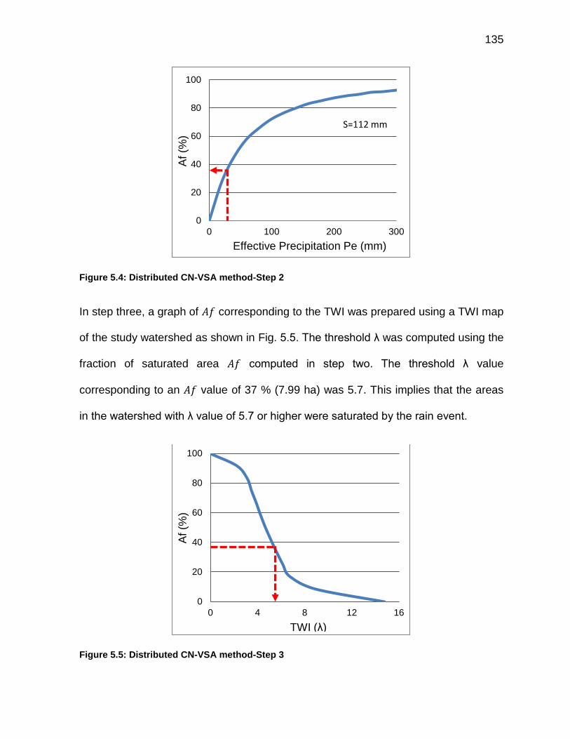
The distributed CNndashVSA approach developed by Lyon et al (2004) simulates the

distribution of saturated areas within the watershed based on VSA hydrology concept

This method is uses SCS-CN approach to estimate runoff amount and Topographic

Wetness Index (TWI) to spatially distribute runoff generating areas within the

watershed This simple method can be easily integrated with existing hydrological

models for predicting the locations of runoff generating areas Recently the relative

saturation of a watershed has been modeled for humid areas using the concept of

water balance dynamics (Manfreda and Fiorentino 2008 Manfreda 2008) This model

38

is based on a stochastic differential equation that allows climatic and physical

characteristics of the watershed to derive a probability density function of surface

runoff

27 Present status

Over the years a number of modeling efforts have been made to understand and

delineate spatial patterns of VSAs During the last two decades increasingly

available computational power has made greater advancements in GIS The

widespread availability of digital geographic data has led to the development of

complex distributed deterministic models These models are based on the distributed

moisture accounting within parts of the landscape for predicting saturation excess

runoff generating areas However the data and computing requirements of these

models restrict their practical application to research studies None of these models

are validated supported by rigorous field tests (Chapi 2009 Pradhan et al 2010)

During the last decade some encouraging attempts have been made to introduce

VSA hydrology into watershed-scale water quality models such as the Soil and Water

Assessment Tool (SWAT) (Easton et al 2008) and Generalized Watershed Loading

Function (GWLF) (Schneiderman et al 2007) However even these process-based

models are too intricate and computationally intensive for field applications (Mills

2008)

In another attempt a water balance-based modified version of the USDAs Soil amp

Water Assessment Tool watershed model SWAT-WB has been developed (Eric

2009) Instead of using the traditional Curve Number method to model surface runoff

39

SWAT-WB uses a physically-based soil water balance In this approach a daily soil

water balance was used to determine the saturation deficit of each hydrologic

response unit (HRU) in SWAT which was then used instead of the CN method to

determine daily runoff volume SWAT-WB model predicts runoff generated from

saturated areas contrary to the traditional SWAT approach However the

performance of this approach needs to be evaluated with field data under various

types of soils land use topography and climatic conditions

Pradhan et al (2010) developed a one-parameter model of saturated source area

dynamics and the spatial distribution of soil moisture The single required parameter

is the maximum soil moisture deficit within the watershed The advantage of this

model is that the required parameter is independent of topographic index distribution

and its associated scaling effects This parameter can easily be measured manually

or by remote sensing The maximum soil moisture deficit of the watershed is a

physical characteristic of the basin and therefore this parameter avoids

regionalization and parameter transferability problems

The majority of present water quality protection procedures assessment methods

and BMPs are developed using the infiltration excess runoff generating theory (Walter

et al 2000) Water quality managers still rely upon popular water quality models such

as the SWAT AGNPS HSPF GWLF etc since these are well established and user-

friendly with their proven nutrient transport and soil erosion transport sub routines

These water quality models are widely used because they are based on the

traditionally acceptable engineering rainfall-runoff approaches (ie the Rational

Method and Curve Number equation) which require little input data Most of these

40

models are primarily based on infiltration excess runoff response mechanism where

soil type and land use are the controlling factors Since dominant factors that affect

variable source area are different than the factors affecting the infiltration excess

runoff generating mechanism models based on infiltration-excess runoff generating

mechanism will show the locations of runoff source areas differently (Schneiderman

et al 2007)

At present VSA hydrology is not widely recognized in the water quality protection

procedures due to the lack of user-friendly water quality models for simulating the

VSA hydrological processes Therefore there is a need to develop new tools to guide

watershed managers in predicting the runoff and correctly locating the critical runoff

generating areas within the watershed for application of BMPs to control non-point

source pollution

28 Towards future developments

The literature shows that there are currently no clearly defined approaches or specific

procedures for monitoring and modeling variable source areas in a watershed Given

that very little data exists on hydrologic processes and their interactions with runoff

generating areas further research is needed to develop a thorough understanding of

this area of hydrology Detailed and extensive fieldwork is required for delineating and

identification of VSAs in watersheds with different types of topography soils climatic

conditions antecedent moisture conditions and land use characteristics

41

Current GIS capabilities can be used at different stages of development of a

hydrologic application Especially important among these is the capability to derive

spatial attributes from various sources such as remote sensing sampling

interpolation digitizing existing maps and the capability to store these attributes in a

geographic database GIS simplifies the collection of climatic and hydrologic input for

use in a model and is easier to apply to a variety of scales from a small field to a

large watershed (Khatami et al 2014) GIS greatly simplifies model setup and that

the use of GIS actually improves model performance (Savabi et al 1995) During the

last two decades the hydrologic community has started moving into a new era of

using GIS-based distributed models Furthermore the GIS platform can be used for

developing models consistent with VSA concept of hydrology for the identification and

quantification of runoff generating areas

Topographic indices derived from Digital Elevation Models are employed to generate

spatially continuous soil water information as an alternative to point measurements of

soil water content Due to their simplicity and physically-based nature these have

become an integral part of VSA-based hydrological models to predict saturated areas

within a watershed

Current monitoring methods of VSAs using digital and analog sensors are limited in

spatial and temporal resolution partly due to the inability of sensors to measure the

temporal variability of surface runoff and partly due to cost and lack of autonomy of

the systems Visits to the field sites are required to collect data and maintain the

sensors (Freiberger et al 2007) Therefore it is necessary to develop new reliable

42

and robust systems for monitoring the spatial and temporal variability of hydrological

parameters and runoff generating areas in a watershed

Recent advances in digital and sensing technology particularly in the area of WSN

systems have enabled real time environmental monitoring at unprecedented spatial

and temporal scales (Mainwaring et al 2002 Trubilowicz et al 2009) These WSNs

have great potential for a wide range of applications including climatic and

hydrological monitoring These WSNs present a significant improvement over

traditional sensors and can be a promising new technology for studying hydrological

response of watersheds in order to monitor spatial-temporal variability of VSAs

(Hughes et al 2006 Chapi 2009)

Information on spatial and temporal distribution of soil moisture is important to identify

VSAs in a watershed Point measurements of soil moisture by conventional soil

sampling and laboratory analysis are slow laborious and expensive (Lingli et al

2009) Furthermore the point measurements of soil moisture are restricted to

describe soil moisture at a small and specific location as spatial distribution of soil

moisture is highly variable over time and space (Stefania 2012 Wood et al 1992)

A non-intrusive geophysical method using Ground Penetrating Radar (GPR) has

been used as a potential alternative method to measure the volumetric water content

(VWC) of shallow soil (Huisman et al 2002) The soil moisture under a range of soil

saturation conditions is estimated with GPR by measuring the reflection travel time of

an electromagnetic wave traveling between a radar transmitter and receiver Soil

43

water content measurements taken with surface GPR reflection methods have shown

good agreement with soil moisture measurements taken by time domain

reflectometry method (Klenk et al 2014) and soil moisture content measured with

capacitance sensors (Van et al 1997 Bradford et al 2014)

Recent technological advances in satellite remote sensing have shown that soil

moisture can be measured by a variety of remote sensing techniques Remotely

sensed data is an important source of spatial information and could be used for

modeling purposes Recent developments in remote sensing technologies are

capable of conducting soil moisture mapping at the regional scale Improvements in

image resolution technology as well as airborne or satellite borne passive and active

radar instruments have potential for monitoring soil water content over large areas

These methods are useful for monitoring soil moisture content for future

environmental and hydrological studies (Chen 2014)

Synthetic-aperture radar (SAR) techniques have the ability to monitor soil parameters

under various weather conditions In the case of unembellished agricultural soils the

reflected radar signal depends strongly on the composition roughness and moisture

content of the soil Many studies have shown the potential of radar data to retrieve

information concerning soil properties using data collected by space and airborne

scatterometers and model simulations (Chan et al 2008 Ouchi 2013) However

water content estimates show limited penetration depth in soils (Lakshmi 2004) and

require a minimal vegetation cover to reduce interference of the radar signal (Jackson

et al 1996) Pizurica et al (2000) observed that temporal radar imagery technique is

very effective for the identification of saturated areas in a watershed

44

The other promising new method of determining soil moisture level is using the

thermal emissions and reflected spectral radiance from soils in the microwave range

from remotely sensed information Thermal emissions from the landscape are

sensitive to soil moisture levels in the upper layer of soil Soil surfaces with higher

moisture content emit lower level of microwave radiation than dry soils (De Jeu et al

2008) Thermal images are generally acquired by aircrafts flying at low altitudes or

can be obtained from high resolution satellites This technique of identifying wet

landscape areas is a promising technology for monitoring VSAs

Another approach to determine soil moisture is to remotely sense the greenness of

the vegetation (DeAlwis et al 2007) Spatial and temporal patterns of vegetation

greenness indices can be derived by measurements taken from a space platform

One such index the Normalized Difference Vegetation Index (NDVI) provides a direct

measurement of the density of green vegetation This index uses strong absorption

by plant leaf pigment (chlorophyll) in the red (R) and contrast between the strong

reflectance measurements of vegetation in the near infra-red (NIR) spectrum

(Petropoulos 2013)

29 Concluding Remarks

VSA hydrology has been universally acknowledged as a basic principle in the

hydrological sciences since 1970 but quantitative understanding of VSA concept is

far from complete and its applications to hydrologic calculations are not fully

developed Very little data exists to physically verify or support different

theorieshydrologic processes and their interactions with runoff generating areas

45

Modeling spatial and temporal variability of VSAs is challenging due to the

involvement of a large number of factors and complex physical processes In spite of

these difficulties and challenges few encouraging attempts have been made to

develop models for quantification and locating runoff generation areas in a

watershed These approaches need to be validated with rigorous field tests to assure

their feasibility and accuracy

At present VSA hydrology is not popular among water quality managers due to a lack

of user-friendly water quality models for simulating VSA hydrologic processes The

majority of current water quality protection practices assessment procedures and

management policies are based on conventional infiltration excess runoff generating

theory Water quality managers still rely on popular water quality models based on

infiltration excess runoff generating mechanism since these are well established and

user-friendly with their proven nutrient transport and soil erosion transport sub

routines However for the areas dominated by saturated excess runoff mechanism

these models may not be able to predict the correct locations of runoff generating

areas

Information concerning saturated areas and spatial soil moisture variations in a

watershed are essential to identify VSAs Advancements in digital WSNs remote

sensing higher resolution satellites aerial photography and increased computational

power may be promising new technologies to monitor spatial and temporal variability

of VSAs Emerging technologies and improved GIS capabilities can be promising

46

tools for the development of new hydrologic applications and VSA-based hydrological

models

210 References

Abraham N and Tiwari K N (1999) Modeling hydrological processes in hillslope

watershed of humid tropics Journal of Irrigation and Drainage Engineering

125(4) 203-211

Agnew L J Lyon S Gerard-Marchant P Collins V B Lembo A J Steenhuis

T S Walter M T (2006) Identification of hydrologically sensitive areas

Bridging the gap between science and application Journal of Environmental

Management 78(1) 63-76

Ambroise B (2004) Variable lsquoactiversquo versus lsquocontributingrsquo areas or periods a

necessary distinction Hydrological Processes 18 1149-1155



Anderson M G Burt T P (1978 b) Toward more detailed field monitoring of

variable source areas Water Resources Research 14(6) 1123-1131



Survey 1(4) 493-498

Barling R D Moore I D Grayson R B (1994) A quasi-dynamic wetness index

for characterizing the spatial distribution of zones of surface saturation and soil

water content Water Resources Research 30(4) 1029-1044

Bernier P Y (1982) VSAS2 a revised source area simulator for small forested

basins University of Georgia Athens Georgia USA Unpublished PhD thesis


69 1541-1552

Betson R P Marius J B (1969) Source areas of storm runoff Water Resources

Research 5 574-582

Beven K (1978) The hydrological response of headwaters and side slopes areas

Hydrological Sciences Bulletin 23(4) 419-437

47

Beven KJ Kirkby MJ (1979) A physically based variable contributing area

model of basin hydrology Hydrological Sciences Bulletin 24(1) 43ndash69

Beven K J (2001) Rainfall-Runoff modeling England The Primer John Wiley and

Sons Chichester

Beven K Wood E F (1983) Catchment geomorphology and the dynamics of

runoff contributing areas Journal of Hydrology 65 139-158

Boughton W C (1987) Evaluating partial areas of watershed runoff American

Society of Civil Engineers Journal of Irrigation and Drainage Engineering

113(3) 356ndash366

Bradford J Thoma M Barrash W (30 June ndash 4 July 2014) Estimating hydrologic

parameters from water table dynamics using coupled hydrologic and ground-

penetrating radar inversion Brussels Belgium 15th International Conference

on Ground Penetrating Radar (GPR) Brussels Belgium 30 Junendash4 July 2014

232ndash237 IEEE 2014

Buda AR Kleinman PJA Srinivasan MS Bryant RB Feyereisen GW (2009)

Factors influencing surface runoff generation from two agricultural hillslopes in

central Pennsylvania Hydrological Processes 23 1295ndash1312

Cappus P (1960) Bassin experimental drsquoAlrance - Etude des lois de lrsquoecoulement

ndash Application au calcul et e la prevision des debits La Houille Blanche A 493-

520


agricultural watershedrdquo Guelph ON Canada University of Guelph PhD Thesis

Chan Y K Koo V C (2008) An introduction to synthetic aperture radar (SAR)

Progress in Electromagnetics Research B (2) 27ndash60

Chaubey I Leh M D Murdoch J Brahan J V Haggard B E (9-12 July 2006)

Quantification of spatial distribution of runoff source areas in an agricultural

watershed Portland Oregon ASABE Annual International Meeting

Chen C Miguel C Chang N Chang L Yuan P (2014) Monitoring

spatiotemporal surface soil moisture variations during dry seasons in Central

America with multi sensor cascade data fusion Journal of Selected Topics in

Applied Earth Observations and Remote Sensing

Chorley R A (1980) The hillslope hydrological cycle Chichester UK Hillslope

Hydrology John Wiley Chapter 1 1ndash42

48

DeAlwis D A Easton Z M Dahlke H E Philpot W D Steenhuis T S (2007)

Unsupervised classification of saturated areas using a time series of remotely

sensed images Hydrology and Earth System Sciences 11 1609ndash1620

De Jeu R Wagner W Holmes T Dolman A J van de Giesen N C Friesen J

(2008) Global soil moisture patterns observed by space borne microwave

radiometers and scatterometers Surveys in Geophysics 29 399ndash420



Dunne T Leopold L B (1978) Water in Environmental Planning W H Freeman

and CO New York NY pp 818

Dunne T Moore T R Taylor C H (1975) Recognition and prediction of runoff-

producing zones in humid regions Hydrological Sciences Bulletin 20(3) 305-

327

Dunne T Black R D (1970 a) An experimental investigation of runoff production in


Dunne T Balck R D (1970 b) Partial area contributions to storm runoff in a small

New England watershed Water Resources Research 6 1296-1311

Easton ZM Fuka D R Walter M T Cowan D M Schneiderman E M

Steenhuis TS (2008) Re-conceptualizing the soil and water assessment tool



Elsenbeer H Vertessy R A (2000) Storm flow generation and flow path

characteristics in an Amazonian rainforest catchment Hydrological Processes

14 2367-2381

Engman E T Arnett J R (1977) Remote sensing applications to a partial area

model Greenbelt NASA Report Goddard Space Flight Centre pp 87

Engman E T Rogowski A S (1974) A partial area model for storm flow synthesis

Water Resources Research 10(3) 464-472

Engman E T (1981) Rainfall-runoff characteristics of a mountainous watershed in

the northeast United States Nordic Hydrology Journal 12 247-264

Eric D W (2009) Development and application of a physically based landscape

water balance in the swat model Ithaca USA Cornell University Master of

Science Thesis

49

Franks SW Gineste P Beven KJ Merot P (1998) On constraining the

predictions of a distributed model The incorporation of fuzzy estimates of

saturated areas into the calibration process Water Resources Research 34

787ndash797

Frankenberger J R Brooks E S Walter M T Walter M F and Steenhuis T S



Freeze R A (1972) The role of subsurface flow in generating surface runoff 2

Upstream source areas Water Resources Research 8(5) 1272-1283

Freeze R A (1974) Streamflow generation Reviews of Geophysics and Space

Physics 12 627-647

Freeze R A (1980) A stochastic-conceptual analysis of rainfall-runoff processes on

a hillslope Water Resources Research 16(2) 391-408

Freiberger T V Sarvestani S S Atekwana E (2007) Hydrological monitoring

with hybrid sensor networks Proceedings of an International Conference on

Sensor Technologies and Applications (SENSORCOMM) 484-489

Gburek W J (1983) Hydrologic delineation of nonpoint source contributing areas

Journal of Environmental Engineering 109(5) 1035-1047

Gburek W J (1990) Initial contributing area of a small watershed Journal of

Hydrology 118 387-403

Gburek WJ Sharpley AN (1998) Hydrologic controls on phosphorus loss from


Gburek W J Drungil C C Srinivasan M S Needelman B A Woodward D E

(2002) Variable-source-area control on phosphorus transport Bridging the gap

between science and design Journal of Soil and Water Conservation 57 534-

543

Godsey S H Elsenbeer R Stallard (2004) Overland flow generation in two

lithologically distinct rainforest catchment Hydrological Processes 14 2367-

2381

Gomi T Sidle R C Ueno M Miyata S Kosugi K (2008) Characteristics of

overland flow generation on steep forested hillslopes of central Japan Journal

of Hydrology 361 275-290

50

Gupta N (2002) Investigation of rainfall-runoff mechanism of field scale Guelph

ON Canada University of Guelph Unpublished PhD Thesis

Guumlntner A Uhlenbrook S Seibert J Leibundgut C (1999) Multi-criterial

validation of TOPMODEL in a mountainous catchment Hydrological Process

13 1603ndash1620

Hart J K Martinez K (2006) Environmental sensor networks A revolution in the

earth system science Earth-Science Reviews 78 177-191

Heerdegen R G Beran M A (1982) Quantifying source areas through land

surface curvature and shape Journal of Hydrology 57 359-373

Hernandez T Nachabe M Ross M Obeysekera J (2003) Modeling runoff from

variable source areas in humid shallow water table environments Journal of

the American Water Resources Association 39(1) 75-85

Hewlett J D (1969) Defense of Experimental Watersheds Water Resources

Research 5(1) 306-316



Hewlett J D Hibbert A R (1967) Factors affecting the response of small

watersheds to precipitation in humid areas Sopper W E and Lull H W

(Eds) Pergamon New York The International Symposium on Forest

Hydrology Pennsylvania State University 275-290


upland basins New York NY Symposium on Interdisciplinary Aspects of

Watershed Management Montana State University Bozeman American

Society of Civil Engineers 65-83

Hoover M D Hursh C R (1943) Influence of topography and soil-depth on runoff

from forest land Transactions of the American Geophysical Union 24 693-697





Horton R E (1937) Hydrologic interrelations of water and soils Proceedings of the

Soil Science Society of America 1 401-429

51



Horton R E Woodward L (1943) Infiltration capacity of some plant-soil complexes

on Utah range watershed lands Transactions of the American Geophysical

Union 24 473-475

Hughes D Greenwood P Porter B Grace P Coulson G Blair G Taiani F

Pappenberger F Snith P Beven K (2006) Using grid technologies to

optimise a wireless sensor network for flood management Boulder Colorado

USA 4th International Conference on Embedded Networked Sensor Systems

389-390

Huisman JA Snepvangers JJ Bouten W Heuvelink G (2002) Mapping spatial

variation in surface soil water content Comparison of ground-penetrating radar

and time domain reflectometry Journal of Hydrology 269 194ndash207

Hursh C R Fletcher P W (1942) Soil profile as a natural reservoir Soil Science

Society American Proceedings 7 480-486

Hursh C R (1944) Report of the sub-committee on subsurface flow Transactions of


Ishaq A M Huff D D (July 27-29 1979 a) Hydrologic source areas A technique

for identifying Fort Collins Colorado USA Colorado State University Fort

Collins Third International Hydrology Symposium on Theoretical and Applied

Hydrology 495-510

Ishaq A M Huff D D (July 27-29 1979 b) Hydrologic source areas B Runoff

simulations Fort Collins Colorado USA Colorado State University Fort Collins

Third International Hydrology Symposium on Theoretical and Applied

Hydrology 511-523

Jackson CR (2005) ldquoJohn D Hewlett (1922-2004) and the Variable Source Area

Conceptrdquo American Geophysical Union Fall Meeting Abstract

Jackson TJ Schmugge J ET Engman (1996) Remote sensing applications to

hydrology Soil moisture Hydrological Sciences Journal 41 517ndash530

Joel A Messing I Segue l O Casanova M (2002) Measurement of surface

runoff from plots of two different sizes Hydrological Processes 161467-1478



52

Khatami S Bahram K (2014) Benefits of GIS Application in Hydrological Modeling

A Brief Summary Journal of Water Management and Research 70 41ndash49

Kim S J Steenhuis T S (2001 b) GRISTORM Grid-Based Variable Source Area

Storm Runoff Model Transaction of the ASAE 44(4) 863-875

Kirkby M J Peel R Chrisholm M Haggett P (1975) Hydrograph modeling

strategies Process in physical and human geography London UK Heinemann

Kirkby M J Chorley R J (1967) Throughflow ovelandflow and erosion

Hydrological Sciences Journal 12 5-21

Kirkby M Bracken L Reaney S (2002) The influence of land use soils and

topography on the delivery of hillslope runoff to channels in SE Spain Earth

Surface Processes and Landforms 27 1459-1473

Kirkby M J Weyman D R (1974) Measurement of contributing area in very small

drainage basins Bristol UK University of Bristol Seminar Series b No 3

Department of Geography

Kirkby M J Callan J Weyman D R Wood J (1976) Measurement and

modeling of dynamic contributing areas in very small catchments University of

Leeds School of Geography Working Paper No 167 pp 40

Klenk P Jaumann S Roth K (2014) Quantitative high-resolution observations of

soil water dynamics in a complicated architecture with time-lapse Ground-

Penetrating Radar Hydrology and Earth System Sciences Discussion 11

12365ndash12403

Knapp BJ Gregory KJ Walling DE (1974) Hillslope through flow observation

and the problem of modeling Fluvial processes in instrumented watersheds

Institute of British geographerrsquo special publication 23ndash32

Kwaad F J P M (1991) Summer and winter regimes of runoff generation and soil

erosion on cultivated loess soils (The Netherlands) Earth Surface Processes

and Landforms 16 653-662

Lakshmi V (2004) The role of satellite remote sensing in the prediction of ungauged

basins Hydrological Processes 18 1029ndash1034

Lamb R Beven KJ Myraboslash S (1997) Discharge and water table predictions

using a generalised TOPMODEL formulation Hydrological Processes 11

1145ndash1168

53

Lamb R Beven KJ Myraboslash S (1998) Use of spatially distributed water table

observations to constrain uncertainty in a rainfall-runoff model Advances in

Water Resources 22 305ndash317

Lane L J Diskin M H Wallace D E Dixon R M (1978) Partial area response

on small semiarid watersheds Water Resources Bulletin 14(5) 1143-1158

Langendoen F D T Keeler-Wolf D Meidinger D Tart C Josse G Navarro B

Hoagland S Ponomarenko J P Saucier A Weakley P Comer (2013)

Guidelines for a Vegetation - Ecologic Approach to Vegetation Description and

Classification (Submitted)

Latron J Gallart F (2007) Seasonal dynamics of runoff-contributing areas in a

small Mediterranean research catchment (Vallcebre Eastern Pyrenees)

Journal of Hydrology 335 194-206

Latron J Gallart F (2008) Runoff generation processes in a small Mediterranean

research catchment (Vallcebre Eastern Pyrenees) Journal of Hydrology 358

206ndash220

Lee M T Delleur J W (1976) A variable source area model of the rainfall-runoff

process based on the watershed stream network Water Resources Research

12(5) 1029-1036




Lingli W John J (2009) Satellite remote sensing applications for surface soil

moisture monitoring A review Frontiers of Earth Science in China 3(2) 237ndash

247

Loganathan GV Shrestha S P Dillaha T A Ross BB (1989) Variable Source


Virginia Water Resources Research Center Bulletin 164 - May 1989




Mainwaring A Culler D Polastre J Szewczyk R Anderson J (2002) Wireless

sensor networks for habitat monitoring New York USA 1st ACM international

workshop on Wireless sensor networks and applications 88-97

54

Manfreda S (2008) Runoff generation dynamics within a humid river basin Natural

Hazards and Earth System Sciences 8 1349-1357

Manfreda S Fiorentino M (2008) A stochastic approach for the description of the

water balance dynamics in a river basin Hydrology and Earth System Sciences

12 1-12

McGuire K J Weiler M McDonnell J J (2007) Integrating tracer experiments

with modeling to assess runoff processes and water transient times Advances

in Water Resources 30 824-837





Generationrdquo Ithaca NY Cornell University Department of Biological and

Environmental Engineering Master of Engineering Report

Mosley M P (1979) Streamflow generation in a forested watershed New Zealand


Moore T Dunne T Taylor C H (1976) Mapping runoff-producing zones in humid

regions Journal of soil and water conservation 31 160-164

Nachabe M (2006) Equivalence between TOPMODEL and the NRSC Curve

Number method in predicting variable runoff source areas Journal of the

American Water Resources Association 42 225-235

Needelman BA Gburek WJ Petersen GW Sharpley AN Kleinman PJA

(2004) Surface runoff along two agricultural hillslopes with contrasting soils

Soil Science Society of America Journal 68 914-923

Ogden FL Watts B A (2000) Saturated area formation on non-convergent

hillslope topography with shallow soils a numerical investigation Water

Resources Research 36 795ndash804

OrsquoLoughlin E M (1981) Saturation regions in catchments and their relation to soil

and topographic properties Journal of Hydrology 53 229-246

OrsquoLoughlin E M (1986) Prediction of surface saturation zones in natural catchment

by topographic analysis Water Resources Research 22(5) 794-804

Ouchi K (2013) Recent Trend and Advance of Synthetic Aperture Radar with

Selected Topics Remote Sensing ISSN 2072-4292 (5) 716-807

55

Petropoulos G P (2013) Remote Sensing of Energy Fluxes and Soil Moisture

Content Publisher CRC Press



572ndash584

Pearce A J (1976) Magnitude and frequency of erosion by Hortonian overland flow

Journal of Geology 84 65-80

Pearce A J Stewart M K Sklash M G (1986) Storm runoff generation in humid

headwater catchments 1 Where does the water come from Water Resources

Research 22(8) 1263-1272

Perrin J L Bouvier C Janeau J L Menez G Cruz F (2001) Rainfallrunoff

processes in a small peri-urban catchment in the Andes Mountains The

Rumihurcu Quebrada (Ecuador) Hydrological Processes 15 843-854

Phillip F Zhao P Samman F A Glesner M (2012) Adaptive Wireless Sensor

Networks Powered by Hybrid Energy Harvesting for Environmental Monitoring

978-1-4673-1975-112 IEEE

Pilgrim D H Duff D D (1978) A field evaluation of subsurface and surface runoff

I Tracer studies Journal of Hydrology 38 299-318

Pionke H B Gburek W J Sharpley A N Tunney H Carton O T Brookes P

C and Johnston A E (1997) Hydrologic and chemical controls on

phosphorus loss from catchments Phosphorus loss from soil to water

Cambridge CAB International Press 225-242

Pizurica A Verhoest N Philips W De Troch F P (2000) Detecting variable

source areas from temporal radar imagery using advanced image enhancement

technique Geoscience and Remote Sensing Symposium IGARSS 2000 IEEE

5 2035-2037

Poret S (2009) Implementation of a Low Power Wireless Sensor Network for

Watershed Monitoring Guelph ON Canada University of Guelph Masterrsquos

Thesis

Qiu Z (2003) A VSA-Based strategy for placing conservation buffers in agricultural

watersheds Environmental Management 32(3) 299-311

Qiu Z MT Walter C Hall (2007) Managing variable source pollution in

agriculture watersheds Journal of soil and water conservation 52(3)115-122

56

Ragan R M (1967) An experimental investigation of partial area contributions

Hydrological Sciences Bulletin 76 241-251

Reinhart K G Trimble G R Eschner AR (1963) Effects on streamflow of four

forest practices in the mountains of West Virginia USDA Forest Service

Northeastern Forest Experiment Station Research Paper NE-I

Riddle M J (1969) Sources of surface runoff on the Canagagigue Creek

Catchment Guelph ON Canada University of Guelph MSc Thesis

Roessel B (1950) Hydrologic problems concerning the runoff in headwater regions

Transactions of the American Geophysical Union 31(3) 431-442

Savabi M R Flanagan D C Hebel B Engel B A (1995) lsquolsquoApplication of WEPP

and GIS-GRASS to a small watershed in Indianarsquorsquo Journal of Soil and Water

Conservation 50(5) 477ndash483

Scherrer S Naef F Faeh A Cordery I (2007) Formation of runoff at the hillslope

scale during intense precipitation Hydrology and Earth System Sciences 11

907ndash922





Sklash M G Stewart M K Pearce A J (June 29 ndash July 2 1986) Storm runoff

generation in humid headwater catchments 2 A case study of hillslope and low-

order stream response Water Resources Research 22(8) 1273-1282




International Meeting Providence Rhode Island June 29 ndash July 2 2008

Shibatani R (1988) Meltwater processes and runoff mechanisms in a small

Precambrian shield watershed during snowmelt Peterborough ON Canada

Trent University MSc Thesis



2278

57



and Embedded Technology and Applications Symposium IEEE 377-386


generation A hillslope-scale field study in east-central Pennsylvania USA


Srinivasan M S Wittman M A Hamlett J M Gburek W J (2000) Surface and

subsurface sensors to record variable runoff generation areas Transactions of

the ASAE 43(3) 651-660

Steenhuis T S and Muck R E (1988) Preferred movement of non-adsorbed


17(3) 376-384

Steenhuis T S Winchell M Rossing J Zollweg J A Walter M F (1995) SCS

runoff equation revisited for variable-source runoff areas Journal of Irrigation

and Drainage Engineering 121(3) 234-238

Stefania M (2012) Soil moisture content estimation using Cosmo-Skymed data

Sesto Fiorentino Italy Final report Scholarship Program ASI-CONAE IFAC-

CNR

Takeuchi K Ishidaira H (1999) Introduction of block-wise use of TOPMODEL and

MuskingumndashCunge method for the hydro-environmental simulation of a large

ungauged basin Hydrological Sciences Journal 44 633ndash646

Tennessee Valley Authority (1964) Bradshaw Creek ndash Elk River A Pilot Study in

Stream-area Factor Correlation Office of Tributary Area Development

Research Report No 4 64

Tennessee Valley Authority (1965) Area-Stream Factor Correlation A Pilot Study in

the Elk River Basin Hydrological Sciences Journal 10(2) 22-37

Tetzlaff D Soulsby C Waldron S Malcolm I Dunne S Lilly A (5-9 December

2005) Testing the variable source area hypothesis using tracers and GIS in a

nested mesoscale catchment San Francisco CA USA American Geophysical

Union Fall Meeting

Troch P Verhoest N Gineste P Paniconi C Meacuterot P Grayson R Bloumlschl

(2000) Variable source areas soil moisture and active microwave observations

at Zwalmbeek and Coeumlt-Dan Spatial Patterns in Catchment Hydrology

Observations and Modelling Cambridge University Press 187-208

58

Troendle C A (1979) A variable source area model for storm flow prediction on first

order forested watersheds Athens Georgia USA University of Georgia

Unpublished PhD thesis

Troendle C A Anderson MC Burt TP (1985) Variable source area models

Chapter 12 Hydrological Forecasting John Willy amp Sons Ltd

Trubilowicz J Weiler K (2009) Viability of motes for hydrological measurement

Water Resources Research 45(4) 23 JAN 2009 DOI 101029

2008WR007046

US Forest Service (1961) Rocky Mountain forest and range experiment Station

1960 Report No 77

Van O Sariowan R Gehrels JC (1997) Ground penetrating radar for determining

volumetric soil water content results of comparative measurements at two sites

Journal of Hydrology 197 316ndash338

Verhoest N E C Troch P A Paniconi C De Troch F P (1998) Mapping basin

scale variable source areas from multitemporal remotely sensed observations of

soil moisture behavior Water Resources Research 34(12) 3235-3244

Vivoni ER Camilli R (2003) Real-time streaming of environmental field data

Computer and Geosciences 29(4) 457-468





Wellen C Arhonditsis G Long T Boyd D (2014) Quantifying the uncertainty of

nonpoint source attribution in distributed water quality models A Bayesian

assessment of SWATrsquos sediment export predictions Journal of Hydrology 519

3353-3368

Wetzel KF (2003) Runoff production processes in small alpine catchments within

the unconsolidated Pleistocene sediments of the Lainbach area (Upper

Bavaria) Hydrological Processes 17 2463-2483



Whipkey R Z (1969) Storm runoff from forested catchments by subsurface routes

International Association of Hydrological Sciences Bulletin 85 773-779

59

Wood E F Lettenmaier DP Zartarian VG (1992) A land surface hydrology

parameterization with sub grid variability for general circulation models Journal

of Geophysics Research 97(D3) 2717-2728

Zavodchikov A B (1965) Computation of spring high water hydrographs using

genetic formula of runoff Soviet Hydrology 5 464-476

Zollweg J A Gburek WJ Pionke HB Sharpley AN (1995) GIS-based

delineation of source areas of phosphorus within agricultural watersheds of the

northeastern USA Proceedings of the IAHS symposium on modeling and

management of sustainable basin scale Water Resources Systems 31ndash39

Zollweg J A (1996) Field study to support hydrologic modeling and analysis of

watershed function at the micro scale Proceedings of Watershed Restoration

Management ndash Physical Chemical and Biological Considerations Middleburg

Virginia USA 129-134

Zollweg J A Gburek W J Steenhuis T S (1996) SMORMOD A GIS-integrated

rainfallndashrunoff model Transactions of the American Society of Agricultural

Engineers 39 1299ndash1307

60

211 Transition to Chapter 3

Watershed monitoring is the most reliable approach for any hydrological or

environmental research Though this approach is time consuming and expensive it is

accurate and trustworthy During last few decades analog type sensor networks have

been used to monitor watersheds for various hydrological and environmental studies

However recent developments in digital and micro sensing technologies and

improved industrial manufacturing processes have made it possible to build small

automatic multi-functional sensors These sensor devices can be used to collect

store and transmit the observations

At present no simple or low cost off-the-shelf solution exists for hydrological

monitoring applications Therefore there is a need for adopting modern technologies

in order to develop an efficient and reliable wireless sensor network system to gather

real-time climatic and hydrological information from remotely located watersheds

Chapter 3 describes the development of a remotely controlled digital wireless sensor

network system for the monitoring and acquisition of climatic and hydrological data

from a distantly located watershed This is the first objective of this research thesis

61

CHAPTER 3

Development and field evaluation of a low cost wireless sensor network system

for hydrological monitoring of a small agricultural watershed

Abstract

Hydrological monitoring and real time access to data are valuable for hydrological

research and water resources management Traditional hydrological monitoring

systems based on analog measurements are prone to noise and cabling

requirements in the field restricts the size of the monitoring area Rapid developments

in digital technology micro-electro-mechanical systems low power micro sensing

technologies and improved industrial manufacturing processes have made Wireless

Sensor Network (WSNs) systems more economical to use This study developed a

remotely operated low cost and robust wireless sensor network system to monitor

and collect climatic and hydrologic data from a small agricultural watershed in harsh

weather conditions near Elora southern Ontario The developed system was

rigorously tested in the laboratory and field and was proven to be accurate and

reliable for monitoring climatic and hydrologic parameters of the watershed

Keywords Hydrological monitoring Wireless Sensor Network Field data collection

Watershed Real-time

31 Introduction

Long-term high quality climatic and hydrological data is essential for hydrological

research and for the implementation of effective water management strategies from

62

field to basin scale Field monitoring and repeated field mapping can be used

effectively for understanding the relationships and interactions between various soil

and environmental parameters of the complex hydrological process (Anderson and

Burt 1978) Monitoring and collection of long-term data from remotely located sites is

time consuming and expensive due to the need for frequent visits to the sites for

maintaining and monitoring the instruments and for downloading data (Freiberger et

al 2007) Although this approach is time consuming and expensive it is accurate and

trustworthy (Chapi 2009) Currently a number of technologies are being used to

acquire hydrological data Accuracy resolution and scalability are some of the major

problems confronting current hydrological monitoring systems These issues need to

be examined and addressed in order to develop an efficient and accurate

hydrological monitoring system

In earlier methods analog type network nodes connected to each other by cables

and number of sensors wired to data loggers were used for hydrological monitoring

The need for this cabling in the field increases cost and restricts the spatial size of the

monitoring area (Oliveira et al 2011) In analog systems converting signals from one

form to another always incurs signal losses Another great disadvantage is that even

with the most careful manufacturing process is that no two analog devices are exactly

the same making the exact duplication of the signal impossible In digital systems

data is converted into binary code and then reassembled back to its original form at

the reception point Since these binary codes can be easily manipulated this method

offers a wider range of options Compared to analog systems digital networks can

collect long-term data at larger scales (Mainwaring et al 2002 Trubilowicz al 2009)

63

A digital WSN system comprised of spatially distributed nodes connected to sensors

communicates bi-directionally to a main location (Jue 2010) As the WSNs do not

require cabling these are cheaper and easier to install in addition to requiring low

maintenance The WSN is built of few to several nodes (known as mote in North

America) where each node is connected to one or more sensors (Sarade et al 2012)

Each sensor network node has four key components (1) The microprocessor amp ADC

(analog to digital converter) (2) Transceiver amp Antenna (3) Memory Unit and (4)

External sensors (Karl and Willig 2005) The individual sensor node consists of a

number of hard wired sensors Each node is wirelessly connected to other nodes

and finally to a central base station (Fig 31)

The WSN possesses great potential for a broad range of applications including

hydrological and environmental monitoring (Cardell et al 2005 Hart et al 2006

Bogena et al 2007 Poret 2009) Recent developments in the field of automatic

sensors and communication systems have further revolutionized the field of

hydrological monitoring The widespread adoption of these devices particularly for

industrial applications has made them extremely cost effective (Song et al 2008)

Because of this these devices can be deployed in large numbers across a watershed

with less human intervention The WSNs are extensively used in many real- world

applications due to their cost effectiveness and deployment flexibility (Philipp et al

2012 Langendoen et al 2013)

64

Figure 31 Typical distributed wireless sensor network system

Sensors used in WSN systems convert physical parameters to electrical signals

WSNs can be used with many diverse types of sensors such as thermal optical

acoustic seismic magnetic infrared and radar These sensors are able to monitor a

wide variety of conditions such as temperature pressure humidity light noise level

movement speed direction and size of an object (Jennifer et al 2008) Sensor nodes

can be used for different purposes including event detection continuous tracking

location sensing etc (Lewis et al 2004 Akyildiz et al 2002)

Unlike other systems WSNs are designed for specific requirements and applications

(Verma 2013) The WSN systems for environmental monitoring are specially

designed to acquire the necessary data at specific time intervals Details of

importance the accuracy of the data and the physical environment of deployment

should be considered while designing the WSN system The WSN system must be

65

designed to withstand weather conditions such as temperature winds rain snow

and pressure or vibration (Hart et al 2006)

During the last decade a number of studies have focused on the field of WSN

technology for environmental monitoring but very few of them are validated by field

tests beyond a few sensor nodes (Szewczyk et al 2004) At present no simple or low

cost off-the-shelf solution exists for hydrological monitoring applications Hence there

is a need for adopting modern technologies to develop efficient and reliable wireless

network systems to gather real-time hydrological information in the present complex

environment

The specific objective of this research is to develop a low cost efficient and remotely

operated WSN system to monitor and collect hydrologic and climatic data from a

watershed The main goal of this study is to acquire real-time hydrologic and climatic

data from a small rural agricultural watershed situated near Elora (Ontario)

32 Design and development of WSN

The design and development of the WSN took place over a four year period from

2007 to 2011 During this period a number of designs with different types of

components were developed and tested Various designs and deployment issues

were identified and resolved during the development process of the WSN

The WSN development took place in three phases In the first phase a WSN system

was designed using hardware from Texas Instruments (TI) The nodes were based

on TI-MSP-TRF6903 boards with a TRF6903 RF transceiver and a MSP430

66

microcontroller The transceiver operates in the 902-MHz to 928-MHz ISM frequency

band and the microcontroller was a 16-Bit ultra-low-power MCU with 60 kB of Flash

memory for data storage

The MPXV70002 vacuum pressure sensor from Freescale was used to capture the

water height and was connected to the ADC port of the TI board The board was

programmed via the MSP430 JTAG connector The MCU Flash memory was erased

and reprogrammed The IAR Systemrsquos Workbench EW430 software package in

combination with the MSP430 JTAG allowed real-time debugging of the code (Poret

2009) The developed WSN with three nodes was tested and evaluated in the

laboratory and the field but it was observed that the communication range of the

nodes was limited and the wireless communication was sensitive to metal fences and

electrical power lines These problems caused noise in pressure readings The large

size of the node boards needed a large waterproof housing unit and antenna which

were difficult to maintain in the field

The WSN system was modified in phase 2 to overcome these problems (Chapi

2009) The hardware components from Crossbow (Xbow) were used to build a new

WSN This system was based on XM2110 motes with built in control and

communication functions Each platform includes an ATmega1281 low-power

microcontroller with a 10-bit ADC and 512 kB of memory and an AT86RF230 RF front

end IEEE 802154 compliant and a ZigBee transceiver with 300 m line-of-sight

transmission range

67

The network gateway consisted of an IRIS mote connected to a USB MIB520CA

interface The Freescale MPXV7002 pressure sensor and the ICT ECH2O soil

moisture sensor were connected to the 51-pin expansion slot through a printed circuit

board (PCB) The interface board passed the sensor data onto a PC The software

tool Mote-View which was designed specifically for the WSN uses XML files to

convert the data from its simple binary input form from the gateway into decimal

values and so these values could be displayed in real-time and saved in a database

The program allowed database dumping whereby collected sensor data is exported

into a text file The text file can be read in Excel and modified with custom calibration

equations

This modified WSN system was tested in the field for communication between nodes

and between nodes and gateway The range of the WSN node as per the Crossbow

IRIS reference manual was greater than 300 m for outdoor conditions and greater

than 50 m for indoor conditions The transmission range of the nodes in the field was

found to be about 250 m at the optimal battery voltage with the range decreasing in

accordance with drops in the battery voltage This system was installed in the study

watershed at the Guelph Turfgrass Institute on the University of Guelph campus

where it performed satisfactorily under a small height of vegetation and level ground

surface conditions The study watershed was monitored and necessary data was

collected from July 2008 to April 2009 for modeling the spatial variability of runoff

generating areas

Despite successful application of this WSN system it still required further

improvements due to its short battery life and interruption of the signal from

68

depressions and tall vegetation Considering this the WSN system was further

modified in phase 3 based on these issues with the objective of improving the

efficiency of WSN system

321 Modification of WSN system (Phase 3)

For further modification of the WSN system in phase 3 updated third generation

MICA2 IRIS 24 GHz nodes XM2110CA were used (Fig 32(1)) This node featured

several new capabilities that enhanced the overall functionality of the WSN system

The communication range of this node was three times better than the previous node

and it has twice as much program memory than previous MICA nodes A Printed

Circuit Board (PCB) was designed and fabricated in order to connect a maximum of

six different kinds of sensors to the 51-pin expansion slot on the node The interface

unit MIB510CA shown in Fig 32 (2) allowed the user to reprogram any node by

plugging the node directly into the base and operating it as part of the root node

interface giving the PC a data conduit of the radio-based sensor network

3211 Sensors

The pressure sensor used for the phase 3 WSN system shown in Fig 32(3) is a new

series of the sensor called the Freescale MPXV7007DP The MPXV7007DP is a

piezo-resistive monolithic silicon dual port pressure sensor It has an output range of

(-2) to 2 kPa with an accuracy of plusmn 25 with 05 to 45 V proportional output

voltage

69

The (E240-40761) 10 cm long (Decagon Devices Inc) 10HS high-frequency soil

moisture sensor (Fig 32(4)) was selected for monitoring soil moisture This

capacitance type sensor has a large sphere of influence to accurately measure the

dielectric permittivity of the soil The electric circuit inside 10HS changes the

capacitance measurement into a proportional millivolt output The high frequency

oscillator removes the soil type sensitivity of the sensor and thus improves its ability

to measure soil moisture in any type of soil

3212 Power supply

The third generation MICA2 nodes require a power range of 17 to 43 V DC supply

for communication within its wireless network After rigorous testing of various

conventional and rechargeable batteries 40 V (45 Ah) lead-acid batteries were

found to be the most reliable for this application This battery lasted for about 30 days

in the field under normal climatic conditions (Fig 32(6)) Solar panels of 14 times 4 times 05

cm with 6 V DC open circuit voltage and a short circuit current output of 100 mA were

used to recharge the battery These panels have 2 solder tabs with 75 cm long

insulated leads to be connected to the batteries and weighs only 27 g Each WSN

node was connected to two solar panels to charge the batteries and maintain the

supply voltage within a specified range to extend the battery life and the WSN

operation as shown in Fig 32(5)

3213 Sturdiness of node assembly

The nodes were made watertight and sturdy to withstand the harsh temperatures

winds and rain for an extended period of time in the field Each wireless node was

70

housed in water tight PVC housing and was attached onto a 30 m long and 25 mm

dia PVC pipe This pipe was attached to a 45 times 45 times 10 cm wooden pedestal The

wooden pedestal was secured in the field by four 29 cm long PVC plugs A glow sign

cone was attached on top of the node for prominent visibility and to protect the PVC

housing from rain and snow A pair of solar panel was attached to this cone This

modified node setup was found to be very sturdy and resistant to harsh climatic

conditions in the field The overall assembly of components of the node in the field is

shown in Fig 32(7)

Figure 32 Components of the developed WSN system (1) IRIS Mote XM2110CA (2) gateway

unit MIB510CA (3) pressure sensor ldquoFreescalerdquo MPXV7007DP (4) soil moisture sensor (E240-

40761) 10HS (5) 6V DC 100 mA solar panel (6) 40 V (45 Ah) lead acid battery (7) assembly of

node in field

3214 Communication connectivity

The nodes were elevated 30 m above ground level to increase communication

connectivity so that the crop height and the depressed areas did not interfere with the

line of sight connectivity between the nodes This increase in the height of the nodes

71

and improved connectivity between them resulted in a decreased number of required

nodes and of the overall cost of the WSN system

Commercial out-of-the-box kits for WSNs were commercially available however the

requirements of reliability and cost-effectiveness for this application led to using

specific hardware and available off the shelf components The hardware components

were purchased directly from the distributors and data acquisition boards for the IRIS

Mote were designed and fabricated in the laboratory in order to increase cost

effectiveness The assembling of WSN components was carried out in the university

workshop to minimize the overall cost of the network

3215 Data visualization tool for WSN

The Mote-View Monitoring Software is developed by Crossbow as a visualization tool

for WSN It allows the users to visualize the data and monitor the status of the

wireless sensor network Each individual node collects data through its sensors and

transmits this data to the base station The data packets received by the base station

are stored in the connected computer in which Mote-View is running Mote-View uses

XML files to convert the data from its simple byte input form from the base station into

decimal values These values are displayed real-time in a window and saved in a

database The program allows for database dumping which exports the collected

sensor data into a text file The text file can be read into Excel and modified with

custom calibration equations

The Mote-View interface has four main tab sections The toolbar tab allows the user

to specify activities and initiate various commands The second tab displays a list of

72

the nodes their health and their deployment status The third visualization tab has

four sub tabs and shows the sensor data as data view command view chart view

and topology view The forth server tab shows incoming messages and a log of the

events

33 Laboratory calibration of nodes

The calibration of soil moisture and pressure sensors was performed in the

laboratory The soil from the experiment field was used to calibrate the soil moisture

sensors Three sensors from a group of sensors were randomly selected for

calibration An oven dry soil with bulk density similar to field conditions was packed

into multiple containers The soil was evenly packed in the containers and the sensor

was inserted in the container during the packing of soil The sensor reading was

noted and the gravimetric method was used to determine the volumetric water

content (θv by volume) of the soil sample Water was added to the container to

raise its water content the sensor reading was recorded and again the water content

was measured by the gravimetric method This procedure was repeated until soil

saturation was achieved The data obtained from the sensor reading and soil water

content was plotted as shown in Fig 33 The following equation fitted to the data

with a determination coefficient (R2) of 09299

θy= 0001x2 - 02063x + 12226 (31)

Where θy= soil moisture content in by volume and x = sensor reading in mV

Similarly three pressure sensors were randomly selected for calibration to determine

the depth of the water A plastic tube was attached to the pressure sensor and placed

73

in a graduated glass cylinder Water was gradually added to this graduated cylinder

to increase the water level from 00 to 20 cm and corresponding sensor readings

were recorded The data collected from this calibration is shown in Fig 34 The linear

equation fitted to this data is presented below and it has a determination coefficient

(R2) of 09891

H = 06072x - 29248 (32)

Where H= depth of water and x stands for sensor reading in mV

Figure 33 Calibration diagram of soil moisture sensor

θ = 0001xsup2 - 02063x + 12226 Rsup2 = 09299

0

10

20

30

40

50

0

50

100

150

200

250

300

350

Soil

mois

ture

θ

( m

3m

3)

VADC (mV)

74

Figure 34 Calibration diagram of pressure sensor

34 Field testing of WSN

The field testing of the WSNrsquos performance was carried out at three different

locations (1) Turf-grass Institute Guelph (ON) (2) Elora Research Station (ERS)

located south of Elora (ON) and (3) Kettle-Creek paired watersheds located within

the southern boundary of the city of London (ON)

The soil moisture and pressure sensor readings obtained by the WSN were verified

by taking manual measurements in the field The height of water above V-notch was

measured manually and soil moisture level of top layer of soil (20 cm) was measured

using digital VG-200 soil moisture meter Fig 35 and Fig 36 show surface runoff

depth and soil moisture readings of node 5 recorded by the WSN and manually for

the storm occurred on 12 September 2011 Similarly WSN readings of node 4

H = 06072x - 29248 Rsup2 = 09891

0

50

100

150

200

250

400

500

600

700

800

900

Head o

f w

ate

r H

(m

m)

VADC (mV)

75

were verified manually on 27 December 2011 (Fig 37 and 38) The comparison

confirmed the proper functioning of the WSN system during field deployment

Figure 35 WSN and manual readings of soil sensor on September 12 2011

Figure 36 WSN and manual readings of pressure sensor on September 12 2011

0

10

20

30

40

50

60

160

0

162

0

164

0

170

0

172

0

174

0

180

0

182

0

Soil

mois

ture

(

m3m

3)

Time (hr)

Sensor reading

Mannual reading

12 September 2011

0

5

10

15

160

0

170

0

180

0

190

0

200

0

210

0

Head o

f w

ate

r

H

(cm

)

Time (hr)

Sensor reading

Mannual reading

12 September 2011

76

Figure 37 WSN and manual readings of soil sensor on December 27 2011

Figure 38 WSN and manual readings of pressure sensor on December 27 2011

0

10

20

30

40

50

60

110

0

112

0

114

0

120

0

122

0

124

0

130

0

132

0

Soil

mois

ture

(

m3m

3)

Time (hr)

Sensor reading Mannual reading

27 December 2012

0

2

4

6

8

10

12

100

0

120

0

140

0

160

0

180

0

200

0

220

0

00

0

Time (hr)

Sensor readings Mannual reading

27 December 2012

Head o

f w

ate

r H

(c

m)

77

35 Field data collection

After successfully testing the WSN system at three different locations (Guelph

University campus Turf Grass Institute Guelph and Kettle Creek paired watershed

near London (ON)) the data collection from a small study watershed of 2162 ha

situated in Elora Research Station (ERS) was carried out from September 2011 to

July 2013 The ERS is located at 43deg 39 N and 80deg 25 W and is about 20 km from

Guelph (ON) The climate in Elora is temperate humid with average annual

precipitation of 875 mm of which about 150 mm falls as snow The elevation of this

agricultural watershed ranges from RL 357 to 378 m with gentle slopes to slopes as

steep as 22 The soil of the study watershed is sandy loam belonging to

hydrological soil group B with soil depth ranging from 060 to 090 m underlain by a

restrictive layer The entire watershed was under the cultivation of hay crop during the

process of data collection

Figure 39 Layout of the study watershed at Elora (Ontario)

78

The study watershed at ERS was divided into 8 sub-watersheds with the help of the

watershed delineating tool of ArcGIS At the outlet of each sub-watershed a V-notch

weir with pressure sensor was installed to measure overland runoff Soil moisture

sensors were installed at the centroids of the sub-watersheds and near all 8 outlet

points A total of 16 soil moisture sensors 8 V-notch weirs with pressure sensors and

6 hopper nodes were installed in this study watershed The watershed at ERS and

the locations of soil moisture sensors and V-notch weirs are shown in Fig 39 A base

station node was attached to a laptop with internet connection and stationed in a

nearby private property in order to power the laptop During spring and fall batteries

lasted for 40 to 45 days depending on weather conditions In the summer batteries

lasted for more than 60 days

Real time access to the field laptop offered the advantage of remotely monitoring the

health and battery level of each node in the field This helped to reduce the number of

site visits as they were only made when the nodes needed to be replaced or

repaired These visits ensured that the WSN was continuously working and that no

data was lost due the repairsreplacement of non-functional nodes Furthermore this

system enabled the user to remotely put the WSN on sleep mode to conserve the

battery power Real time access also enabled the user to adjust the data sampling

interval accordingly to rainy or dry periods Since relevant data was to be collected

during rainy periods the sampling interval was shortened remotely compared to the

sampling interval during dry weather This not only helped to conserve the battery life

but also helped to avoid the collection of unnecessary data

79

The soil moisture sensorrsquos readings were converted from mV to soil moisture

percentage by using the calibration equation 31 Similarly the pressure sensorrsquos

readings collected by the WSN system were converted to water depth by using

calibration equation 32 A flow hydrograph of each field segment was developed to

compute the total flow generated by the field Rainfall and temperature data were

collected from ERS weather station located about 500 m from the study watershed

Surface runoff and soil moisture monitoring started in September 2011 and continued

until July 2013 Soil moisture levels and runoff generated from eight sub-watersheds

was monitored for 45 rainfall events for simulation and mapping of runoff generating

areas in the study watershed

The field measurements of a rainfall event dated 01 June 2012 are plotted in Fig

310 Rainfall started at 500 am and total rainfall for the event was 4603 mm The

maximum daytime temperature was 137 degC The average soil moisture of the

watershed at the beginning of the rainfall (θ) was 014 (by volume) and runoff initiated

after 43 minutes when soil moisture (θ) reached 043 (saturation) This indicated that

the initial abstraction (Ia) of this rainfall event was 61 mm The peak discharges of

0041 m3s 0013 m3s and 0161 m3s were recorded at 700 pm at the outlets of

sub-watershed 4 and 6 as well as at the end of the watershed By analysing the

runoff hydrograph data it was calculated that this rainfall event generated 2456 m3 of

overland flow and the coefficient of runoff was 2928

80

Figure 310 Field observations of rainfall and runoff event dated June 01 2012

The continuously recorded field data of soil moisture rainfall and temperature during

the month September 2012 is shown in Fig 311 There were 6 major rainfall events

and a maximum of 2576 mm of rain recorded on 08 September 2012 The average

soil moisture of the study watershed was about 14 (by volume) at the beginning of

the month and increased to 42-45 during rainfall events The graph also shows

daily maximum and minimum temperatures during the month The maximum

temperature of 288 degC was recorded on 03 September and the minimum of 06 degC on

24 September 2012 Field observations of precipitation soil moisture and

temperature during the year 2012 are shown in Fig 312

0

5

10

15

20

250000

0005

0010

0015

0020

0025

0030

0035

0040

40

0

70

0

100

0

130

0

160

0

190

0

220

0

10

0

40

0

Precipitation Sub watershed 1 Sub watershed 2Sub watershed 3 Sub watershed 4 Sub watershed 5Sub watershed 6 Sub watershed 7 Sub watershed 8

Dis

charg

e (

m3s

)

Pre

cip

itation (

mm

)

Time (hr) 01 June 2012

81

Figure 311 Field observations of precipitation soil moisture and temperature during

September 2012

Figure 312 Field observations of precipitation soil moisture and temperature during year 2012

0

10

20

30

40

50

600

10

20

30

40

50

60

70

80

1-S

ep

4-S

ep

7-S

ep

10

-Se

p

13

-Se

p

16

-Se

p

19

-Se

p

22

-Se

p

25

-Se

p

28

-Se

p

Pre

cip

itation (

mm

)

Tem

p (

degC)

and s

oil

mois

ture

(m

3m

3)

Date

Precipitation Max temperature Min Temperature Soil moisture

September 2012

0

20

40

60

80-10

0

10

20

30

40

50

60

70

1-M

ay

31-M

ay

30-J

un

30-J

ul

29-A

ug

28-S

ep

28-O

ct

27-N

ov

27-D

ec

Tem

p (

degC)

and s

oil

mois

ture

(

m3m

3)

Date

Precipitation Max Temperature Min Temperature Soil moisture

Pre

cip

itation (

mm

)

Year 2012

82

The field data of soil moisture and discharge for 10 rainfall events in the fall of 2011

were successfully recorded During the year 2012 data for 4 spring events 10

summer events and 10 fall events were collected During the year of 2013 field data

for 3 spring and 8 summer rainfall events were recorded for simulating and mapping

of runoff generating areas in the study watershed It was observed that the installed

WSN system worked accurately with minimum maintenance for extended periods of

time

36 Summary and conclusions

This research has provided an overview of the development of an integrated WSN

system for monitoring climatic and hydrologic parameters of a remotely located

agricultural watershed This system was designed to acquire store and transmit

climatic and hydrological data from a remotely situated agricultural watershed The

designed WSN system was comprised of an advanced wireless network technology

which together with the internet facilitates the communication of field data between

the study site and client in real time This WSN system was calibrated in the

laboratory and tested at three locations in southwestern Ontario Canada Field scale

testing demonstrated that the system was robust enough to work under adverse

weather conditions such as high winds rain and snow The developed WSN system

was reliable and accurate in monitoring the climatic and hydrologic data of the

watershed This system was installed in a remote agricultural field near Elora (ON)

where it worked satisfactorily with minimum maintenance and enabled continuous

data collection for two years

83

The advantage of this system is that it can be accessed from anywhere by any

computer connected to the internet Remote data collection and maintenance

considerably reduced the need for site visits which significantly reduced the

monitoring cost Although this WSN system was specifically tailored for a project

focused on mapping the VSAs in a small rural agricultural watershed it is still flexible

to use in a variety of contexts Thus this WSN system will prove to be a useful and

flexible tool for future hydrological research

37 References

Akyildiz IF Su W Sankara subramaniam Y Cayirci E (2002) Wireless sensor

networks a survey Computer Networks 38 393ndash422

Anderson M G Burt T P (1978) Toward more detailed field monitoring of variable

source areas Water Resources Research 14(6) 1123-1131

Bogena H Huisman JA Oberdoumlrster C Vereecken H (2007) Evaluation of a

low-cost soil water content sensor Journal of Hydrology 344 32ndash42

Dropbox

httpswwwdropboxcombusinesshome=trueamp_tk=sem_goog_bamp_kw=dropbo

x|eamp_net=gamp_ad=39420846102|1t1amp_camp=sem_goog_b_ca_eng_top_exactamp

mkwid=s4ZfKezUs|pcrid|39420846102|pmt|e|pkw|dropbox|pdv|c|ampkw=dropbox|

eampmuid




Gutierrez JA Callaway EH Barrett RL (2004) Low-Rate Wireless Personal

Area Networks Enabling Wireless Sensors New York IEEE Press IEEE

802154

Hart J K Martinez K (2006) Environmental Sensor Networks A revolution in the


84

Jennifer Y Mukherjee B Ghosal D (2008) Wireless sensor network survey

wwwelseviercomlocatecomnetComputer Networks 52 2292ndash2330

Jue Y (2010) Design and implementation of large-scale wireless sensor networks

for environmental monitoring applications University of North Texas

Dissertation Prepared for the Degree of Doctor of Philosophy

Chapi K (2009) Monitoring and Modeling of Runoff Generating Areas in a Small

Agriculture Watershed Guelph ON Canada University of Guelph PhD Thesis

Karl H Willig A (2005) Protocols and architectures for wireless sensor networks

Wiley

Langendoen F D T Keeler-Wolf Meidinger D Tart D Josse C Navarro G

Hoagland B Ponomarenko S J Saucier Weakley A Comer P (2013)


Classification Washington DC Ecological Society of America (Submitted)

Lewis FL D J Cook S K Das (2004) Wireless sensor networks Smart

Environments Technology Protocols and Applications Wiley

LogMeIn

httpssecurelogmeincomwelcomefreeremotecontroladestination=welcomefreer

emotecontrolaampwtsrch=1amputpk=logmeinamporiginid=345693ampmcomb


sensor networks for habitat monitoring 1st ACM international workshop on

Wireless sensor networks and applications ACM 88-97

Martin T Peterson J (2005) Wireless sensor network for watershed analysis

Guelph ON Canada University of Guelph School of Engineering Report



Philipp F Ping Z Faizal A Samman Manfred G (2012) Adaptive Wireless

Sensor Networks Powered by Hybrid Energy Harvesting for Environmental

Monitoring 978-1-4673-1975-112 IEEE



Thesis

85


Influencing Factors amp Types of Sensor Network ISSN International Journal of

Innovative Technology and Exploring Engineering (IJITEE) 3(5) 2278-3075

Sarade SS ACJoshi Sachin S Patil and ANShinde (2012) Wireless

temperature monitoring system using wireless sensor networks International

Journal of Advanced Research in Electronics and Communication Engineering

(IJARECE) 1(4) 46-51



and Embedded Technology and Applications Symposium IEEE RTAS08 377-

386



47(6) 34-40

Trubilowicz J Kan C Markus W (2009) Viability of motes for hydrological

measurement Water Resources Research Vol 45 W00D22 doi 101029

2008WR007046

86


In the preceding chapter an innovative remotely operated low cost and robust WSN

system was developed to monitor and collect the climatic and hydrologic parameters

from an agricultural watershed Chapter 4 describes the second objective of this

research to conduct an experimental field study to investigate the significance of the

climatic and hydrological factors affecting the spatiotemporal variability of runoff

generating areas For this analysis the climatic and hydrological data was collected

using the WSN system developed in the previous chapter

87

CHAPTER 4


watershed in southern Ontario

Abstract

Prediction and identification of runoff generating areas is important for developing

watershed management strategies to mitigate non-point source pollution Spatial and

temporal variability of runoff generating areas are very complex and depend on

multiple climatic and hydrological factors The majority of the previous research

studies describe great variability in the dominant factors responsible for runoff

generation Furthermore very limited field data is available to physically verify the

dominance of various controlling factors

In this study a small watershed divided into eight sub-watersheds was monitored for

two years by using a remotely operated Wireless Sensor Network (WSN) system Soil

moisture and runoff data for 7 spring 18 summer and 20 fall season rainfall events

were collected to identify the significance of factors affecting the spatial and temporal

variability of runoff generating areas The results showed strong seasonal influence

on runoff generating areas Rainfall amount initial soil moisture conditions and rainfall

intensity were found to be the most significant factors affecting the runoff generating

areas

Keywords Runoff coefficient Runoff generating areas Spatial and temporal

variability Saturation excess runoff Nonpoint source pollution

88

41 Introduction

Management of Non-point Source Pollution (NPS) necessitates accurate modeling of

the rainfall-runoff process in the humid and well-vegetated rural watersheds The

rainfallndashrunoff transformation is a nonlinear and very complex process as it depends

on a number of climatic and hydrologic parameters Even though a wide variety of

different approaches and a large number of models have been developed to

understand the spatial and temporal dynamics of rainfall-runoff relationships a unified

approach is still missing (Ponce 2014)

Rainfall properties soil characteristics land use climatic conditions topography

surfacesubsurfacegroundwater hydrology and geology are the main factors involved

in controlling the spatial-temporal variability of runoff generation (Das 2009)

Moreover the factors that influence the spatial and temporal variability of runoff also

depend on the dominant runoff generating mechanism as the main factors that

control infiltration excess runoff generation are different than the factors that affect

saturated excess runoff process (Vertessy et al 2000 Schneiderman et al 2007)

In case of infiltration excess mechanism runoff depends mainly on rainfall intensity

and total rainfall amount is not an important parameter Further when rainfall

intensities are much larger or smaller than the infiltration capacity of soils the initial

soil moisture conditions are also not critical Contrary to this for regions where

saturation excess runoff generation is the dominant process total rainfall amount is a

controlling factor and rainfall intensity does not play major role (Kostka et al 2003

Castillo et al 2003)

89

Runoff coefficient is one of the most widely used key concepts in engineering

hydrology to describe rainfall-runoff relationships Analysis of runoff coefficients is

useful in understanding the transformation of rainfall into event-based runoff The

concept of event runoff coefficient dates back to the beginning of the 20th century

(Sherman 1932) but it is still an existing research issue in hydrology (Ralf et al

2009) The majority of previous research studies indicate great variability in the

dominant factors responsible for runoff generation process (Weiler et al 2003) The

main limitation on the analysis of runoff generation research has been the lack of field

data on rainfall-runoff events to evaluate the impact of various factors affecting runoff

generating areas (Kuang et al 2012)

During the last decade researchers have investigated the significance of the soil

moisture dynamic on runoff generation by monitoring small experimental watersheds

and have observed that the wetness condition of the landscape before the rainfall

event is an important factor in the runoff generation (Longobardia et al 2003 Zehe

and Bloschl 2004 Aronica and Candela 2004) A study by Brocca et al (2009)

suggests that the rainfall amount rainfall intensity and the antecedent wetness

condition (AWC) are the most significant factors affecting the runoff generation and

out of these three factors AWC is the most important one

In this study a remotely operated Wireless Sensor Network (WSN) system was used

in a small rural agricultural watershed to continuously monitor soil moisture conditions

and runoff generated by different parts of the watershed Climatic and hydrologic data

for 7 spring 18 summer and 20 fall events from September 2011 to July 2013 were

collected The main objective of the study was to investigate the significance level of

90

the correlation of runoff coefficient with rainfall amount initial soil moisture content

rainfall intensity five day antecedent rainfall and rainfall duration to describe the

annual and seasonal variability of runoff generating areas

42 Materials and Methods

421 Study area

The experimental field study was conducted in a 2162 ha agricultural watershed in

the Elora Research Station (ERS) of University of Guelph located at 43deg 39 N and

80deg 25 W in Ontario Canada (Fig 41) Elora has a humid continental climate with

warm summers and no dry season The temperature typically varies between -139

degC to 214 degC and is rarely below -18 degC or above 28 degC The average annual

precipitation in the study region is about 875 mm of which about 150 mm falls as

snow The elevation of the watershed ranged from RL 357 to 378 m with gentle to

slopes as steep as 22 The general slope of the watershed is towards northwest

side where it outlets in to a small creek

Figure 41 Layout of study watershed and sub-watersheds in Elora Research Centre

91

Soil samples collected from fifteen locations in the study watershed were used to

determine the physical properties as given in Table 41 The surface soil (0 to 20 cm)

was classified as sandy loam texture (Hydrologic Soil Group B) based on the particle

size distribution The procedure outlined by Black et al (1965) was used for the

mechanical analysis of the soil Bulk density was determined using undisturbed core

samples A Guelph Permeameter (GP) was used to obtain in-situ measurements of

field saturated hydraulic conductivity (Ks) The depth of the restrictive layer was

determined by using an auger and ranged from 60 to 90 cm During the study period

the experimental watershed was under the cultivation of hay crop

Table 41 Characteristics of field soil

Soil Sand Silt Clay Bulk

density Ks

() () () (kgm3) (ms)

Sandy loam 61 29 10 1190 318 x 10-8

422 Monitoring the climatic and hydrologic variables

The Digital Elevation Model (DEM) of the study watershed was developed by the

Lidar (Light Detection and Ranging) survey This DEM was used to obtain principal

geomorphic features such as hill slope and drainage channels in the study

watershed The watershed was divided into 8 sub-watersheds using the flow path

pattern A remotely operated Wireless Sensor Network (WSN) system was installed

in the watershed to continuously monitor soil moisture and runoff sensors Soil

moisture sensors were installed at two locations in each sub-watershed and runoff

92

was monitored at the outlet of each sub-watershed A base station node was

attached to a laptop with internet connection and stationed in a nearby shelter to

store and communicate the collected data At the outlet of each sub-watershed a V-

notch weir with pressure sensor was installed to measure overland runoff A total of

16 soil moisture sensors 8 V-notch weirs with pressure sensors and 6 hopper nodes

were installed in this study watershed The detailed layout of the monitoring locations

of soil moisture sensors and V-notch weirs are shown in Fig 42

Figure 42 Monitoring locations of soil moisture sensors and V-notch weirs

The (E240-40761) 10HS high-frequency 10 cm long soil moisture sensor was

selected and used for monitoring the soil moisture This capacitance type sensor has

a large sphere of influence to accurately measure the dielectric permittivity of the soil

93

The electric circuit inside 10HS changes the capacitance measurement into a

proportional millivolt output The high frequency oscillator of this sensor removes the

soil type sensitivity of the sensor and thus improves its ability to measure soil

moisture in any type of soil V-notch weirs were used to measure flow at the outlet of

each sub-watersheds The head of water over the V-notch crest was measured with

piezo-resistive monolithic silicon dual port Freescale MPXV7007DP pressure

sensors

Rainfall and temperature data were collected from the ERS weather station located

500 m from the experimental watershed Rainfall data collected using tipping bucket

rain gauge permitted the characterization of each event in terms of rainfall intensity

duration and rainfall amount Storms were defined as events with more than 5 mm of

precipitation Events were considered distinct if they were separated by at least 12

hours The rainfall events were generally characterized by relatively short and intense

convective storms although few long duration rainfall events were also recorded



was monitored for 45 rainfall events This includes 7 events during spring 18 during

summer and 20 during the fall season Observed runoff was considered as saturated

excess surface runoff when the rainfall intensity was less than the saturated hydraulic

conductivity of soil (Ks) and infiltration excess type when the rainfall intensity

exceeded the Ks

94

423 Analysis procedure

The data collected during the field observation were used to determine the dominant

factors affecting the runoff generating areas The runoff coefficient was used as an

index of runoff generating areas and the time of ponding was used as an index to

identify the time when the sub-watershed started runoff contributing runoff to the

outlet of the watershed The factors evaluated include rainfall amount initial soil

moisture rainfall intensity 5-day antecedent rainfall and rainfall duration The factors

affecting seasonal variability in runoff coefficient due to seasonal variations were also

investigated Spring season covered the period from February 1 to May 31 summer

season from June 1 to September 31 and fall from October 1 to January 31

(Dickinson et al 2007)

The influence of the factors affecting runoff generating area was evaluated by using

various statistical tests Statistical Analysis System (SAS) software (SAS Institute

2004) was used to perform correlation and multi-variable regression analysis The

appropriateness of the multiple regression model as a whole was tested by the F-test

The statistical tools used include linear regression coefficient of determination (R2)

root mean square error (RMSE) Pearson product-moment correlation coefficient (r)

test and p-test Coefficient of determination is a statistical measure of how close the

data are to the fitted regression line The root mean square error (RMSE) was used

as an indicator of the differences between the values predicted by a model or an

estimator and the actual observed values Pearson product-moment correlation

coefficient (r) is an indication of strength and direction of the linear relationship

between two sets of data It is defined as the sample covariance of the variables

95

divided by the product of their (sample) standard deviations A correlation greater

than plusmn 08 is generally described as strong whereas a correlation less than plusmn 05 is

generally described as weak (Masaaki 2013) The p-test is a statistical method used

for testing a hypothesis within a population or a proportion within a large population

43 Results and Discussion

Ontario hydrology exhibits seasonal patterns that strongly influence the rainfall-runoff

process The physical condition of a watershed varies spatially and temporally due to

number of climatic and hydrologic factors Therefore the rainfall soil moisture at the

beginning of runoff event rainfall intensity rainfall during the last five-day rainfall

duration and runoff generated at the watershed outlet for 45 rainfall events are

presented in Table 42 Runoff co-efficient is considered as minimum runoff

generating area (MRGA) for this analysis and the probability of exceedance of the

storms (return period) is calculated by using equation (41) suggested by Weibull

(1951)

119875 =119898

(119899+1) (41)

Where

P = probability of exceedance in years m = rank of position and n = number of

samples

96

Table 42 Main characteristics of 45 observed rainfall-runoff events

Event Date

Initial soil

moisture

Rainfall during last 5-

day

Rainfall Max

rainfall intensity

Time of ponding

Rainfall duration

Runoff

Minimum runoff

generating area

(MRGA)

Return period

(m3m

3) (mm) (mm) (mmh) (min) (min) (mm) (Year)

Spring

1 23-Apr-12 0312 69 71 38 89 360 307 434 11

2 30-Apr-12 0185 00 105 26 32 540 134 127 12

3 03-May-12 0331 105 297 97 16 240 1486 500 51

4 08-May-12 0276 297 161 66 53 180 219 136 18

5 10-May-13 0217 00 150 58 55 720 546 364 16

6 21-May-13 0199 102 409 94 16 300 1882 460 92

7 28-May-13 0263 32 386 86 46 780 1478 383 77

Summer

8 01-Jun-12 0140 20 460 72 43 960 1136 247 153

9 12-Jun-12 0232 00 62 62 18 60 021 34 11

10 26-Jul-12 0133 15 206 182 15 180 124 60 22

11 31-Jul-12 0164 252 83 23 124 540 011 13 11

12 05-Aug-12 0185 83 181 134 34 180 093 51 19

13 09-Aug-12 0217 181 318 118 68 480 251 79 58

14 27-Aug-12 0129 00 53 23 80 180 023 43 10

15 04-Sep-12 0101 00 139 56 166 420 047 34 14

16 08-Sep-12 0176 139 258 66 169 840 363 141 29

17 14-Sep-12 0134 00 144 36 84 360 091 63 15

18 18-Sep-12 0162 144 206 123 112 420 182 88 21

19 22-Sep-12 0277 206 98 43 62 240 019 19 12

20 29-Sep-12 0128 00 156 63 24 480 077 49 17

21 10-Jun-13 0114 38 457 96 69 1260 1171 256 115

22 30-Jun-13 0147 00 228 72 162 360 107 47 26

23 05-Jul-13 0174 228 281 127 138 540 190 68 38

24 08-Jul-13 0326 351 148 103 241 300 085 58 15

25 27-Jul-13 0094 00 277 175 33 120 244 88 35

26 31-Jul-13 0246 277 357 106 151 720 488 137 66

27 12-Sep-11 0104 00 120 67 28 120 026 22 13

Fall

28 13-Oct-11 0339 222 283 87 69 480 541 192 42

29 14-Oct-11 0295 283 472 87 31 600 1663 353 230

30 19-Oct-11 0212 472 179 45 72 360 157 88 18

31 22-Nov-11 0146 06 95 21 192 480 026 27 12

32 27-Nov-11 0254 95 154 30 119 1080 271 176 16

33 29-Nov-11 0325 154 484 63 85 1140 1348 279 460

97

Event Date Initial soil

moisture


day

Rainfall Max

rainfall intensity

Time of ponding

Rainfall duration

Runoff

Minimum runoff

generating area

(MRGA)

Return period

(m3m


34 04-Dec-11 0336 484 265 64 48 360 548 207 31

35 14-Dec-11 0237 00 215 53 39 420 199 93 23

36 27-Dec-11 0228 21 82 40 62 180 038 46 11

37 13-Oct-12 0167 00 288 131 182 600 351 122 46

38 20-Oct-12 0196 00 122 53 112 300 070 57 14

39 23-Oct-12 0274 122 245 71 104 1020 345 141 27

40 26-Oct-12 0317 245 271 24 418 1500 598 221 33

41 28-Oct-12 0332 516 197 55 67 600 226 115 20

42 12-Nov-12 0285 72 98 26 89 360 031 32 12

43 02-Dec-12 0238 76 216 92 29 180 493 228 24

44 16-Dec-12 0257 66 120 33 244 900 057 48 14

45 20-Dec-12 0211 120 108 31 142 600 033 30 13

Runoff from the majority of the rainfall events was generated by saturated excess

runoff generating mechanism because the rainfall intensity for only 8 events

exceeded the saturated infiltration capacity of the soil

The data show that the event rainfall amount ranged from 532 mm to 4840 mm

Maximum rainfall of 4840 mm occurred on 29-Nov-11 The maximum rainfall

intensity of this event was 631 mmhr producing 1348 mm of runoff resulting in a 28

of MRGA The rain event with the least rain (532 mm) occurred on 27-Aug-12

This three-hour long rain event with rainfall intensity of 232 mmhr with relatively dry

initial soil moisture conditions generated 023 mm (4972 m3) of runoff and registered

4 value of MRGA In the spring season the maximum amount of rainfall occurred

on 21-May-13 A total of 409 mm of rainfall was recorded within 5 hour time span

with a maximum intensity of 937 mmhr This event generated 1882 mm (4069 m3)

of runoff and resulted 46 of MRGA The maximum rainfall during the summer

98

season was measured on 31-July-13 when 3568 mm of rainfall with a rainfall

intensity of 1061 mmhr generated 488 mm (1055 m3) of runoff with 14 of MRGA

The soil moisture content before the rain events during spring summer and fall

seasons ranged from 020 to 036 009 to 033 and 017 to 034 m3m3 respectively

The maximum 5-day antecedent rainfall amount of 5163 mm measured on 28-Oct-12

was the result of two successive storms on 23-Oct-12 and 26-Oct-12 This pre-event

rainfall increased the soil moisture content of the watershed to 033 m3m3 The

summary statistics of 45 observed rainfall events is given in Table 43

Table 43 Statistical summary of 45 observed rainfall-runoff events

Rainfall

Initial soil moisture

Max rainfall

intensity

Rainfall during last

5-day

Rainfall Duration

Runoff generating

area

(mm) (m3m3) (mmh) (mm) (min) ()

Minimum 532 009 214 000 60 13

Maximum 4840 034 1820 5163 1500 500

Mean 2156 022 728 1211 503 143

Median 1969 022 657 761 420 88

Standard deviation 1185 007 388 1402 335 130

These data also show a large variability in MRGA due to variations in the climatic and

hydrologic conditions of the watershed The summary statistics of seasonal variation

of MRGAs is given in Table 44

99

Table 44 Seasonal statistics of minimum runoff generating area

Minimum runoff generating areas ()

Spring Summer Fall

Minimum 127 13 27

Maximum 500 256 353

Mean 344 80 136

Median 383 59 118

Standard deviation 152 68 95

The data show that the runoff generating area is strongly influenced by seasons

MRGA during the spring season were maximum and varied from 127 to 500

The highest MRGA of 500 occurred during a rain event on dated 3-May-12 with

rainfall amount of 297 mm and maximum rainfall intensity of 967 mmhr The initial

soil moisture at the beginning of this event was 033 m3m3 and 5-day antecedent

rainfall was 105 mm The MRGA of 127 was registered during the rainfall event

dated 30-Apr-12 The low value of MRGA was due to small rainfall amount and lower

pre-event soil moisture content

The MRGA during summer varied from 13 to 256 with the average of 8

During this season about 75 percent of rainfall events exhibited MRGAs less than 10

and 40 percent of the events had MRGA less than 5 Four rainfall events for

which the runoff generating area was greater than 10 were storms with high rainfall

intensity and large rainfall amount Two rainfall events that produced MRGA of about

25 were large events with rainfall amount of more than 45 mm Maximum MRGA of

256 was produced by a severe rainfall event on 10-June-13 with rainfall amount of

4571 mm and maximum rainfall intensity of 962 mmhr The lowest MRGA of 133

was recorded for a 9 hour long rain event dated 31-July-12 with rainfall of 829 mm

100

and maximum rainfall intensity of 227 mmhr The watershed before the start of this

rain event was relatively dry with soil moisture content of 016 m3m3

For fall events the MRGA ranged from 27 to 353 with an average value of 136

The minimum MRGA of 27 occurred on 22-Nov-11 This was due to very low

initial soil moisture content (014 m3m3) at the beginning of the event During this

event 953 mm of rain fell over eight hours with maximum rainfall intensity of 214

mmhr The rainfall event producing the largest MRGA of 353 occurred on 14-Oct-

11 with rainfall depth of 4716 mm During this event the landscape was relatively

wet with soil moisture content of 029 m3m3 and 5-day antecedent rainfall of 283

mm The maximum rainfall intensity during this event was relatively high (874

mmhr)

101

431 Factors affecting the variability of runoff generating area

In this study seasonal and annual variability of runoff generating areas was further

explored by means of investigating the possible effect of rainfall amount initial soil

moisture rainfall intensity five day antecedent rainfall and rainfall duration on runoff

coefficient (minimum runoff generating area)

4311 Effect of rainfall amount

The annual and seasonal variation of minimum runoff generating areas with rainfall

amount is presented in Fig 43

Figure 43 Relationship between minimum runoff generating area and rainfall amount

These data show that over the year MRGAs increase with an increase in rainfall

amount The relationship between MRGA and rainfall amount is the strongest for the

summer season (R2=081) followed by fall (R2=073) and spring (R2=026) During the

0

10

20

30

40

50

0 10 20 30 40 50

Min

imum

runoff

genera

ting a

rea (

)

Rainfall (mm)

Spring Summer Fall

Rsup2=073

Rsup2=047

Rsup2=081

R2=026

102

spring season the MRGA did not show strong relationship with rainfall amount This

was due to high initial soil moisture conditions The evapotranspiration losses during

this season were relatively small These conditions resulted in low infiltration During

summer relatively dry soil profile in the watershed due to low soil water content at the

beginning of the rainfall resulted high infiltration and low MRGA An increase in

rainfall amount resulted more runoff high runoff coefficient and strongest relationship

between MRGA and rainfall amount For the fall season the relationship between

MRGA and rainfall amount is strong but weaker than summer The MRGA for a

particular rainfall amount during fall season is about 8 less than during summer

season The variability within this season is due to variability in the initial soil moisture

conditions at the beginning of rainfall event

4312 Effect of initial soil moisture content

The variability in the MRGA with initial soil moisture content over the years and for

various seasons is shown in Fig 44

These data shows that MRGA increases in proportion to the increase in initial soil

moisture at the beginning of a rainfall event However during the spring the MRGA

did not show any relationship with initial soil water content During early part of this

season all the rainfall events generated high value of MRGA This was due to high

initial soil moisture conditions and impeded infiltration due to presence of frost layer at

a shallow depth in the soil profile

103

Figure 44 Relationship between minimum runoff generating area and initial soil moisture

During late spring period the absence of frost layer in the soil profile enhanced

infiltration and reduction in MRGA For summer events there is a strong positive

relationship (R2= 078) between MRGA and initial soil water content For most of the

rainfall events during this season the initial soil conditions were relatively dry ranged

from 009 to 028 m3m3 resulted in less runoff amount and reduced MRGA For

majority of rainfall events the MRGA did not exceed greater than 15

For the fall season the MRGA again showed strong positive relationship with initial

soil water content but the temporal variability was more than summerrsquos variability

These results show that during the summer and fall seasons initial soil moisture

content plays an important role on the magnitude of minimum runoff generating area

These results also agree with the observations of Castillo et al (2003) that the runoff

0

10

20

30

40

50

000 005 010 015 020 025 030 035 040

Min

imum

runoff

genera

ting a

rea (

)

Initial soil moisture (m3m3)

Spring Summer Fall

Rsup2=078

Rsup2=067

Rsup2=050

Rsup2=0001

104

response for the saturation excess type of runoff generating mechanism depends on

the wetness condition of the landscape

4313 Effect of rainfall intensity

Figure 45 shows annual and seasonal change in MRGA with rainfall intensity

Figure 45 Relationship between minimum runoff generating area and maximum rainfall

intensity

These data show that the MRGA increases with rainfall intensity however the trends

are stronger for summer and fall seasons than the spring season The maximum

rainfall intensity for the spring and fall events did not exceed 105 mmhr and for

majority of events it was less than 8 mmh whereas the MRGA of 5 out of 7 events

were more than 35 The low value of the determination coefficient (R2) suggests

that rainfall intensity does not have any significant effect on MRGA for spring rainfall

0

10

20

30

40

50

0 3 6 9 12 15

Min

imum

runoff

genera

ting a

rea (

)

Rainfall intensity (mmh)

Spring Summer Fall

Rsup2=036

Rsup2=061 Rsup2=018

Rsup2=071

105

events For all the summer events with maximum rainfall intensity is less than 10

mmhr and MRGA is less than 10 Only two events with maximum rainfall intensity

of about 135 mmhr generated 25 value of MRGA For the fall season the MRGA

showed mixed trend with maximum rainfall intensity Majority of the rainfall events

with maximum rainfall intensity is less than 9 mmhr generated less than 20 values

of MRGA However for three events with maximum rainfall intensity of 6 mmhr the

MRGA was more than 20 and for one event close to 30 This was due to either

high initial soil water content or high rainfall amount

4314 Effect of five-day antecedent rainfall amount

Figure 46 shows the temporal variations in MRGA with five-day antecedent rainfall

amount Over the annual time frame the relationship between MRGA and five-day

antecedent rainfall amount is very weak or practically insignificant with a coefficient of

determination of 016 The MRGA showed relatively higher correlation with 5-day

antecedent rainfall amounts during summer and fall seasons than spring with R2

value of 064 and 053 respectively For spring events the MRGA varies in a very

narrow range and more than 35 though the maximum five-day antecedent rainfall

amount does not exceed 10 mm This was due to very wet soil moisture condition

and five-day rainfall has no significant effect on the pre-event wetness conditions

During late spring summer and early fall period the five-day antecedent rainfall

amount affects the MRGA area by affecting the initial soil moisture condition During

winter period five-day antecedent rainfall amount has minimum effect on soil wetness

and MRGA

106

Figure 46 Relationship between minimum runoff generating area and five-day antecedent

rainfall

4315 Effect of rainfall duration

The effect of rainfall duration on the MRGA over the year and during spring summer

and fall seasons is presented in Fig 47

These data show relatively week relationship between MRCA and rainfall amount

relative to other factors affecting MRGA Over the annual time frame virtually no

relationship (R2=010) exists between the MRGA and rainfall duration During the

spring season for majority of the rainfall events the MRGA is greater than 30 Two

events for which MRGA is less than 15 occurred during late spring period when the

soil was relatively dry For the summer and fall events the MRGA increases with

rainfall duration but the relationship was moderately positive with (R2) of 052 and

0

10

20

30

40

50

0 10 20 30 40 50

Min

imum

runoff

genera

ting a

rea (

)

5-day antecedent rainfall (mm)

Spring Summer Fall

Rsup2=053

Rsup2=016

Rsup2=064

R2=007

107

041 respectively During summer and early fall periods the rainfall intensities were

generally high and an increase in rainfall duration resulted an increase in RGA

Figure 47 Relationship between minimum runoff generating area and rainfall duration

The summary statistics of the relationship of MRGA with rainfall amount initial soil

water content maximum rainfall intensity 5-day antecedent rainfall and rainfall

duration is given in Table 45 These data show that over the annual time frame

rainfall amount and initial soil moisture conditions are the most important factors For

spring period the MRGA is controlled by rainfall amount and maximum rainfall

intensity For summer and fall period all the factors are important to describe the

magnitude of MRGA

0

10

20

30

40

50

0 400 800 1200 1600

Min

imum

runoff

genera

ting a

rea (

)

Rainfall duration (min)

Spring Summer Fall

Rsup2=00008

Rsup2=041

Rsup2=010

Rsup2=052

108

Table 45 Summary of correlation of various factors with minimum runoff generating area

Minimum runoff generating area

Spring Summer Fall Annual

(R2) (R2) (R2) (R2)

Rainfall amount (mm) 026 081 073 047

Initial soil moisture (m3m3) 001 078 067 032

Rainfall intensity (mmh) 036 071 061 018

5-day antecedent rainfall (mm) 007 064 053 016

Rainfall duration (min) 000 052 041 010

The variability of the MRGA was further investigated by means of Pearson product-

moment correlation coefficient statistics and the results are presented in Table 46

Table 46 Statistical correlation of various factors with minimum runoff generating area

Pearson Correlation Coefficients N = 45

Prob gt |r| under H0 Rho=0

RC P IMC I 5-DAR D

MRGA |r|

1 06856 05657 04243 04000 03162

p-value lt0001 00181 00231 06783 00398

P |r| 06856

1 00389 04391 01718 04999

p-value lt0001 07997 00025 02593 00005

IMC |r| 05657 00389

1 -02848 05825 01730

p-value 00181 07997 0058 lt0001 02557

I |r| 04243 04391 -02848

1 00109 -02168

p-value 00231 00025 0058 09434 01525

5-DAR |r| 04000 01718 05825 00109

1 00725

p-value 06783 02593 lt0001 09434 06361

D |r| 03162 04999 01730 -02168 00725

1 p-value 00398 00005 02557 01525 06361

MRGA=Minimum runoff generating area P= Rainfall (mm) IMC= Initial soil moisture content (m

3m

3)

I= Rainfall intensity (mmh) 5-DAR= 5 day antecedent rainfall (mm) D= Duration of event (min)

109

This correlation matrix shows that the rainfall amount initial soil moisture rainfall

intensity and rainfall duration exhibit Pearsons coefficients of correlation |r| of 06856

05657 04243 and 03162 respectively with p-values lt 005 This means that there

is sufficient evidence to believe that these factors have significant positive correlation

with the MRGA Contrarily the p-value of the five-day antecedent rainfall factor is

06783 with |r| value of 04000 suggests that this factor does not have an effect on

MRGA Ranking of these factors based on the strength of |r| indicates that rainfall

amount is the most significant factor followed by initial soil moisture content and

maximum rainfall intensity

432 Multivariable Linear Regression analysis

To develop a possible relationship between the MRGA and the factors affecting it a

Multi Variable Linear Regression (MVLR) analysis was performed over the annual

and seasonal data The relationship obtained is presented in Table 47 The

regression results show that MRGA can be estimated with very good accuracy during

summer season good accuracy during spring season and fall winter season and with

reasonable accuracy over annual time frame using rainfall amount initial soil

moisture content rainfall intensity five-day antecedent rainfall and rainfall duration

parameters The data also show that the MRGA has strong seasonal dependency

110

Table 47 Simulated multivariable linear regression equations and their descriptive statistics

Equation n R2 RMSE

F-value

PrgtF value

Spring MRGA = 025189-000732(P) + 007504(IMC) + 007484(I)-00144(5-DAR) -000030(D)

7 07554 01811 062 07408

Summer MRGA = -007990 + 000273(P) + 031853(IMC) + 000135(I) -000225(5-DAR) + 000013(D)

18 09051 00258 2288 lt00001

Fall MRGA = -008397 + 000628(P) + 038510(IMC) - 000168(I) -000021 (5-DAR) )- 000001(D)

20 07851 00501 1035 00003

Annual MRGA = -012978 + 000853(P) + 091420(IMC) - 000545(I) -000326(5-DAR)- 000007(D)

45 05415 00931 921 lt00001

P= Rainfall (mm) IMC= Initial soil moisture content (m3m

3) I= Rainfall intensity (mmh) 5-DAR= 5-day

antecedent rainfall (mm) D= Duration of event (min) n= Number of observation RMSE = Root mean square error

The developed MLRV model for the summer season with a p-value of lt00001 and

R2 of 090 shows a statistically best fit regression model between MRGA with rainfall

amount initial soil water content maximum rainfall intensity 5-day antecedent rainfall

amount and rainfall duration The regression analysis for spring and fall seasons

shows R2 values of 075 and 078 and RMSE values of 018 and 005 respectively

The higher RMSE associated with spring season can be attributed to large standard

deviation of the unexplained variance of the response variable The developed

regression model incorporating all 45 observed events for the prediction of MRGA

over the annual time frame with a R2 value of 054 and p-value of lt00001

demonstrates a statistically significant relationship (Table 47)

111

Multivariable regression analysis between time of ponding (Tp) and rainfall amount

initial soil water content maximum rainfall intensity five-day antecedent rainfall and

rainfall duration for spring summer and fall showed no significant correlation (Table

48) However the developed regression equation using all 45 observed events

exhibited a R2 value of 045 and p-value of lt005 The developed annual equation

and their descriptive statistics are presented in Table 48

Table 48 Simulated multivariable regression equation for time of ponding and descriptive

statistics

Equation n R2 RMSE

F-value

PrgtF value

Annual Tp=667932-35703(P) ndash 1319377(IMC) + 27013(I) + 11860(5-DAR) + 01966(D)

45 04546 01811 6085 00002

433 Relation of minimum contributing areas with basin moisture index and

storm index

The concept of basin moisture index (Dickinson and Whiteley 1970) and storm index

(Arteaga et al 1973) and their relationship with runoff contributing areas were also

investigated using the data obtained from observed events Again the runoff

coefficient was used as an index of minimum contributing area

Dickinson and Whiteley (1970) studied effect of antecedent wetness conditions and

rainfall amount on minimum contributing area Their study reveals that the minimum

contributing area varies from 1 to 50 percent and the majority of events have

minimum contributing areas below 10 percent with a median value of 5 percent The

112

relationship for the basin moisture index in Eq 42 proposed by Dickinson and

Whiteley is given as

119872 = 119872119886 +119875

2 (42)

Where M = the basin moisture index at the beginning of the storm in cm

Ma = the soil moisture stored in the upper 70 cm of soil and

P = the precipitation depth (cm)

The basin moisture index computed by using the relationship described above is

shown in Fig 48 The shape of this relationship is similar to the one proposed by

Dickinson and Whiteley (1970)

Figure 48 Relationship between minimum contributing area and basin moisture index

0

10

20

30

40

50

00 100 200 300 400

Min

imum

contr

ibuting a

rea (

)

Basin moisture Index M (cm)

Spring Summer Fall

113

The data suggest that the relationship between the minimum contributing area and

the basin moisture index is nonlinear in nature and that the basin moisture index

value of approximately 25 cm behaves as a threshold value The minimum

contributing area is relatively constant up to 25 cm value of basin moisture index and

less than 10 of the area contributes runoff for more than 80 of rainfall events

The minimum contributing area showed a marked and rapid increase in basin

moisture index greater than the threshold value These data also show that all the

spring events have a basin moisture index greater than the threshold value and a

minimum contributing area greater than 16 Most of the summer and spring season

events have minimum contributing areas less than 12

Figure 49 presents the relationship between the minimum contributing area and the

storm index proposed by Arteaga et al (1973) The storm index (Eq 43) is defined

as

119878119868 = 119860 +119875

2 (43)

Where SI is storm index (inch) A is antecedent rainfall (inch) and P is total storm

rainfall (inch)

The relationship between the minimum contributing area and the storm index is

similar in form to the relationship between minimum contributing area and basin

moisture index

114

Figure 49 Relationship between minimum contributing area and storm index

These data show that the storm index up to 25 inches exhibits a linear relationship

with minimum contributing area After the threshold values an increase in SI values

results a rapid increase in the minimum contributing area The data also show all of

the spring events have SI indices greater than the threshold value of 25 inch with

minimum contributing area between 15 to 45 Most of the summer and fall season

events constitute runoff contributing area of less than 10 of the total watershed

area

434 Description of spatial and seasonal minimum runoff generating areas

To investigate seasonal and spatial variability in minimum runoff generating areas

three median rainfall events one each from spring summer and fall were selected for

analysis The summary of various climatic characteristics and hydrological responses

0

10

20

30

40

50

00 05 10 15 20 25 30 35 40

Min

imum

contr

ibuting a

rea (

)

Storm Index SI (inch)

Spring Summer Fall

115

of the eight sub-watersheds for this rain event are shown in Table 49 The spring rain

event dated 10-May-13 was four hours long with a rainfall amount of 1501 mm and

maximum rainfall intensity of 576 mmhr The maximum and minimum temperatures

on this spring day were 176degC and 69degC respectively

Table 49 Summary of climatic and hydrological data for spring event dated 10-May-13

S1 S2 S3 S4 S5 S6 S7 S8

Sub-watershed area (ha) 302 306 271 442 206 15 356 129

Five-day antecedent rainfall (mm) 0 0 0 0 0 0 0 0

Initial soil moisture (m3m

3) 023 021 024 02 018 019 017 026

Total rainfall (mm) 1501 1501 1501 1501 1501 1501 1501 1501

Max rainfall intensity (mmhr) 576 576 576 576 576 576 576 576

Runoff (m3) 186 181 170 214 104 74 168 82

Peak runoff (m3s)

140 X 10-4

115 X 10-4

94 X 10-4

217 X 10-4

64 X 10-4

33 X 10-4

150 X 10-4

94 X 10-4

Runoff generating area () 4103 3941 4179 3226 3363 3287 3144 4235

Runoff contribution to the watershed () 1578 1535 1442 1815 882 628 1425 696

These data show that for 10-May-13 rainfall event the runoff generating area of sub-

watersheds ranged from 3144 to 4235 During this rainfall event all parts of the

watershed contribute to the runoff at the outlet The reason is that pre-event soil

moisture of sub-watershed 8 was the wettest among all eight sub-watersheds (026

m3m3) and it contributed 696 of the total watershed runoff with a runoff generating

area of 4235 Sub-watersheds 3 and 1 were second and third in the ranking with

runoff generating areas 4179 and 4103 respectively The runoff generating

area of sub-watershed 7 was minimum (3144 ) and it generated 168 m3 of runoff

and contributed 1425 of the total watershed runoff This shows that the areas with

116

higher soil moisture or the wetter areas within the watershed generated the larger

amount of runoff

The summer event dated 05-July-13 was six hours long with a rainfall amount of

2813 mm and a maximum rainfall intensity of 127 mmhr The five-day antecedent

rainfall for this event was 231 mm and the maximum and minimum temperatures for

this summer day were 237degC and 165degC respectively The summary of various

climatic characteristics and the hydrological responses of the eight sub-watersheds

for this rain event is shown in Table 410

Table 410 Summary of climatic and hydrological data for summer event dated 05-July-13

S1 S2 S3 S4 S5 S6 S7 S8




3) 019 016 018 015 016 017 014 021



Runoff (m3) 76 66 61 65 38 27 40 37

Peak runoff (m3s)

84 X 10-4

73 X 10-4

60 X 10-4

127 X 10-4

42 X 10-4

23 X 10-4

92 X 10-4

43 X 10-4



These data show that the runoff generating areas of sub-watersheds varies from 399

to 1020 The soil moisture of the sub-watersheds before the rainfall event of

ranged from 014 to 021 m3m3 Sub-watershed 8 was the wettest among all sub-

watersheds with a soil moisture content of 021 m3m3 and contribution 902 to the

total watershed runoff with a MRGA of 1020 The lower initial soil water content of

117

014 m3m3 of sub-watershed 7 resulted in the least MRGA of 399 During this

event this sub-watershed generated 40 m3 of runoff and contributed 976 of the

total runoff

A fall rain event dated 13-Oct-12 lasted for five hours with a rainfall amount of 2884

mm and maximum rainfall intensity of 1310 mmhr The summary of various climatic

characteristics and hydrological responses of the eight sub-watersheds for this rain

event are shown in Table 411

Table 411 Summary of climatic and hydrological data for fall event dated 13-Oct-12

S1 S2 S3 S4 S5 S6 S7 S8




3) 021 018 019 015 017 016 014 023



Runoff (m3) 130 114 105 124 66 47 90 64

Peak runoff (m3s)

69 X 10-4

64 X 10-4

56 X 10-4

95 X 10-4

43 X 10-4

29 X 10-4

74 X 10-4

36 X 10-4



The data Table 411 show that the average minimum area generating runoff is 124

and the sub-watershed area generating runoff ranges from 877 to 1720 Prior to

the initiation of the rainfall event the soil moisture content of the sub-watersheds

ranged from 014 to 023 m3m3 The peak runoff discharges at the outlet of sub-

watersheds was between 29 x 10-4 to 95 x 10-4 m3s Sub watershed 1 produced the

highest amount of runoff (130 m3) and contributed 1757 of total watershed runoff

118

followed by watershed 4 with runoff of 124 m3 and a contribution of 1676 of the

total runoff Sub-watersheds 2 and 3 ranked third and fourth and sub-watershed 6

contributed the least amount (47 m3) of runoff and contributed 635 of total

watershed runoff

Comparison of the results in Tables 49 410 and 411 also show that sub-watershed

8 has the maximum MRGA and sub-watershed 7 has the minimum MRGA for any

event during the study period These results also show that rainfall intensity during

the spring does not have any significance effect on runoff generating areas whereas

higher rainfall intensity results in larger MRGA during the summer and fall The data

also shows that MRGA increases with an increase in initial soil water content Due to

wetness conditions of the watershed the MRGA are large during spring season

compared to summer and fall seasons These result also suggest that though the soil

and land use of sub-watersheds were same the minimum runoff generating area also

exhibits seasonal and spatial variability

44 Conclusions

Based on the results reported in this study the following conclusions can be drawn

Runoff generating areas exhibits strong seasonal variability Rainfall amount is the

most significant factor affecting minimum runoff generating areas followed by initial

soil moisture and rainfall intensity Five-day antecedent rainfall and rainfall duration

have minimum impact on the minimum runoff generating area Rainfall amount and

maximum rainfall intensity are the dominant factors affecting minimum runoff

generating areas during spring period During summer and fall period dominant

119

factors affecting minimum runoff generating area includes rainfall amount and initial

soil water content followed by maximum rainfall intensity five-day antecedent rainfall

and rainfall duration There are threshold basin soil moisture index and storm index

below which the minimum contributing are is relatively insignificant Above these

indices the minimum contributing area exhibits an exponential increase

45 References

Aronica G Candela A (2004) ldquoA regional methodology for deriving flood frequency

curves FFC in catchments with uncertain knowledge of soil moisture conditionsrdquo

Osnabruumlck Germany University of Osnabruumlck 1147ndash1183

Arteaga F E and Rantz S E (1973) Application of the source-area concept of

storm runoff to a small Arizona watershed Journal of Research US Geological

Survey 1(4) 493-498

Black CA Evans DD White JW Ensminger LE Clark FE (1965) Methods

of soil analysis part I Agronomy No 9 American Society of Agronomy

Wisconsin USA Madison pp 886

Brocca L Melone F Moramarco T Singh V P (2009) Assimilation of Observed

Soil Moisture Data in Storm Rainfall-Runoff Modeling Journal of Hydrologic

Engineering 14(2) 153ndash165

Castillo V M Gomez-Plaza A Martinez-Mena M (2003) ldquoThe role of antecedent

soil water content in the runoff response of semiarid catchments A simulation

approachrdquo Journal of Hydrology 284 114ndash130

Das G (2009) Hydrology and Soil Conservation Engineering including Watershed

Management New Delhi PHI Learning Private Limited



Dickinson WT RP Rudra GW Wall SM Kazim (2007) Possible Impacts on

Soil Erosion and Sediment Yield Planning for Extremes Ontario Chapter of the

Soil amp Water Conservation Society 23-69

120

Kostka Z Holko L P Miklanek (2003) ldquoAnalysis of rainfall-runoff events in a

mountain catchmentrdquo Interdisciplinary approaches in small catchment

hydrology Monitoring and research Paris Technical Documents in Hydrology

UNESCO 67 19ndash25

Kuang B Mahmood H S Quraishi M Z Hoogmoed W B Mouazen A M van

Henten E J (2012) Sensing Soil Properties in the Laboratory In Site and On-

Line Advances in Agronomy 114(1) 155-223

Longobardia A Villania P Graysonb RB Westernb AW (2003) On the

relationship between runoff coefficient and catchment initial conditions The

Modelling and Simulation Society of Australia and New Zealand

Masaaki K (2013) Human-Computer Interaction Part 4 Las Vegas NV USA 15th

International conference HCI international Proceedings

Ponce VM (1989) Engineering Hydrology Principles and Practices Prentice Hall

second edition online

Ralf M Guumlnter B (2009) A regional analysis of event runoff coefficients with

respect to climate and catchment characteristics Austria Water Resources

Research 45 1-19

SAS (Statistical Analysis Systems) Institute 2004 SAS Software and Userrsquos Guide

Cary NC Statistical Analysis Systems Institute

Sherman L (1932) Streamflow from rainfall by unit hydrograph method Chicago

Engineering News Records 501ndash505

Vertessy R Elsenbeer H Bessard Y Lack A (2000) ldquoStorm runoff generation at

La Cuencardquo Spatial patterns in catchment hydrology Cambridge UK

Cambridge University Press 247ndash271

Weibull W (1951) A statistical distribution function of wide applicability Journal of

Applied Mechanics 18(3) 293-297

Weiler M McGlynn B L McGuire K J McDonnell J J (2003) ldquoHow does rainfall

become runoff A combined tracer and runoff transfer function approachrdquo Water

Resources Research 39(11) 1315-1327

Zehe E Bloschl G (2004) ldquoPredictability of hydrologic response at the plot and

catchment scales Role of initial conditionrdquo Water Resources Research 40 doi

1010292003WR002869 ISSN 0043-1397

121


The third objective of this research study was to appraise the existing methods and

models to assess their strength and gaps in quantification and delineating the VSAs

The literature suggests that very few models have been developed to simulate

hydrological processes based on VSA concepts Recently there has been some re-

conceptualization of widely-used water quality models to account for VSA hydrology

The majority of these models are continuous long-term hydrologic simulation models

The distributed CNndashVSA approach developed by Lyon et al (2004) is one of the

promising new methods to simulate the distribution of saturated areas within the

watershed based on VSA hydrology concepts This method was selected for detailed

evaluation as it is an event-based method This is a physically-based method and

uses SCS-CN approach to predict runoff amount and spatial extent of saturated

areas This method distributes runoff generating areas by using topographic wetness

index approach

In chapter 5 the distributed CN-VSA method was evaluated and modified to account

for seasonal changes in potential maximum retention (S) The modified distributed

CN-VSA method was applied to the study watershed to simulate runoff amount and

spatial extent of saturated areas using observed data presented in the preceding

chapter to evaluate its feasibility and accuracy of mapping the VSAs

122

CHAPTER 5


estimation of spatial distribution of Variable Source Areas

Abstract

Many of the current watershed models employ Soil Conservation Service Curve

Number (SCS-CN) approach based on soil and land use for runoff simulation These

models implicitly assume that runoff is generated by the Hortonian process and

therefore they are unable to correctly account for the effects of topography or

moisture distribution in a watershed

The distributed CN-VSA method is based on SCS-CN approach to estimate runoff

amount and uses the Topographic Wetness Index (TWI) to spatially distribute runoff

generating areas within the watershed The size of the saturated watershed areas

and their spatial locations are simulated by assuming an average annual value of

potential maximum retention However the literature indicates large seasonal

variation in the value of potential maximum retention

This paper focuses on the evaluation and modification of the distributed CN-VSA

method to account for the seasonal changes in the potential maximum retention

Simulated results indicate that the modified distributed CN-VSA method performed

better than the distributed CN-VSA method to predict runoff amount as well as size

and spatial distribution of runoff generating areas This method is simple and can be

incorporated into non-point source pollution models

123

Keywords Saturation excess runoff Variable source area SCS runoff curve

number Topographic wetness index Nonpoint Source Pollution

51 Introduction

Saturation excess is one of the dominant mechanisms of overland flow generation in

humid and well-vegetated regions (Dunne 1978 Ward 1984) Predicting the locations

of saturated areas and the corresponding risks of generating surface runoff is

important for developing watershed management strategies to mitigate non-point

source pollution and its impacts

Saturation excess runoff occurs when soil becomes saturated from below after the

water table rises to the land surface either from excess rainfall or from shallow lateral

subsurface flow Precipitation over these saturated areas results in overland flow

(Dunne and Leopold 1978) This is opposed to the Hortonian theory which assumes

that runoff occurs when the precipitation rate exceeds the maximum soil infiltration

capacity (Horton 1933) Furthermore Hortonian overland flow does not occur at low

rainfall intensities and it is often assumed to take place uniformly over the landscape

However the portion of the watershed susceptible to saturation excess runoff varies

seasonally as well as within a storm thus these areas are generally termed as


1999 Walter et al 2000) VSAs generally develop along the lower portions of

hillslopes topographically converging or concave areas valley floors shallow water

table areas and adjoining the streams (Amerman 1965)

124

The number of models based on the VSA concept of watershed response are

reported in the literature including TOPMODEL (Beven and Kirkby 1979) DHSVM


al 1996) etc These models have varying degrees of complexity and are based on

distributed moisture accounting within the segments of a watershed but these

models are rarely used as they require copious calibration and large amount of input

data (Pradhan et al 2010) Over the last decade some encouraging attempts have

been made to introduce VSA hydrology in the watershed scale water quality models

such as the Soil and Water Asessment Tool SWAT-VSA (Easton et al 2008) and the

Generalized Watershed Loading Function (GWLF) (Schneiderman et al 2007)

However these models need to be validated with rigorous field tests Moreover

these models are somewhat more complicated and computationally intensive than

most engineering applications warrant (Mills 2008)

The majority of hydrologic and non-point source pollution models have the option of

using the SCS-CN method for estimating surface runoff from a storm rainfall The

main advantage of this method is that it incorporates most of the factors affecting

runoff generation such as soil class land use surface condition and antecedent soil

moisture amount (Ponce and Hawkins 1996 Mishra and Singh 2003a Mishra et al

2004(b) Mishra et al 2005) Despite several identified problems such as lumping the

watershed parameters in a single parameter a lack of peer reviewed justification and

uncertainty in runoff estimates the CN method is extensively used to estimate

surface runoff (Soulis et al 2009) from ungauged watersheds Steenhuis et al (1995)

suggested that the theoretical basis of the SCS-CN method is valid for both Hortorian

125

and saturation excess runoff generating mechanisms (Hjelmfelt 1980) However the

majority of water quality models use the SCS-CN method based on soil infiltration

characteristics and land use for runoff simulation Therefore these models are not

able to correctly locate the runoff generating areas as the main factors that control

infiltration excess runoff generation mechanism are different from the factors that

control VSAs (Schneiderman et al 2007)

Ever since the inception of the VSA concept of runoff generation topography has

been considered as an important factor affecting the hydrological processes in

watershed hydrology (Hewlett and Hibbert 1967) In hilly watersheds with moderate to

steep topography the gravity component dominates the hydraulic potential and the

characteristics of the terrain are vital variables to determine the watershed response

and distribution of water to rainfall inputs (Rodriguez et al 1979 Beven and Kirkby

1979 OrsquoLoughlin 1986 Anderson et al 1992) Various topographic indices of

wetness are being used to generate spatially continuous soil water information for

identifying saturation excess areas as an alternative to point measurements of soil

water content (Hassan et al 2007 Moore et al 1993 Western et al 1999) Moreover

due to their simplicity and physically-based nature topographic indices have become

an integral part of VSA-based hydrological models (Yong et al 2012)


promising new methods based on VSA concept to simulate the aerial distribution of

saturation excess runoff This is a physically-based method and uses a traditional

SCS-CN approach to predict runoff volume and spatial extent of saturated areas and

distributes runoff source areas within the watershed using a Topographic Wetness

126

Index (TWI) approach This simple method can be integrated with existing

hydrological models for predicting the locations of runoff generating areas based on

the VSA concept In the distributed CN-VSA method potential maximum retention is

assumed to be constant throughout the year However field observations indicate a

large variation between the annual average potential storage and potential maximum

retention value for spring summer and fall seasons Therefore the distributed CN-

VSA method needs modification in order to move from a constant potential maximum

retention to a seasonal variable potential maximum retention

The main objectives of this study are to modify and evaluate the distributed CN-VSA

method Both distributed CN-VSA method and the modified distributed CN-VSA

method were applied to a small agricultural watershed Simulated results of runoff

and its aerial distribution in the watershed for spring summer and fall rainfall events

were compared with observed field data to evaluate their feasibility and accuracy of

mapping the VSAs in a watershed

52 Description of distributed CNndashVSA method

The distributed CNndashVSA method divides a watershed into two parts The saturated

part generating runoff and the remaining unsaturated part infiltrates and do not

contribute to runoff This method estimates the saturated fraction of watershed by

using the SCS runoff curve number method and aerially distributes runoff source

areas through the watersheds by application of TWI approach

127

521 Predicting the saturated fractional area of watershed

The rainfall-runoff equation used by the SCSndashCN method (USDA-SCS 1972) for

estimating the depth of direct runoff from storm rainfall is given as

119876 =(119875minus119868119886)2

(119875minus119868119886+119878) Which is valid for Pgt 119868119886 and 119876 = 0 119891119900119903 119875 le 119868119886 (51)

Where

Q = Runoff in mm P = Rainfall in mm 119868119886 = Initial abstraction in mm and S = Potential

maximum retention in mm

This form of CN equation was proposed by Mockus (1949) after reviewing results

from many small experimental watersheds (Wildermuth et al 2009 Rallison 1980)

This equation is widely used in hydrological engineering in spite of its empirical

nature The effective precipitation Pe is the part of precipitation that contributes to

surface runoff and is defined as

Pe = P minus 119868119886 (52)

Eq (51) can be rewritten as

119876 =1198751198902

119875119890+119878 (53)

Steenhuis et al (1995) suggested that Eq (53) can be used to determine saturation

excess runoff that results from saturated soils The underlying principle of this VSA

interpretation of the SCS-CN equation is that the fractional area Af of the watershed

128

generating runoff can be estimated from the ratio of runoff depth (∆Q) to precipitation

depth (∆Pe) given by the following equation

119860119891 = ∆Q

∆Pe (54)

The runoff generating area according to Eq (54) is equal to the derivative of Q with

respect to Pe Differentiating Eq (53) with respect to Pe using partial fraction

decomposition the fraction of watershed generating area can be computed

119876 = 119875119890 minus 119878 + 1198782

119875119890+119878 (55)

The differentiation results in

119860119891 = 1 minus 1198782

(119875119890+119878)2 (56)

Eq (56) is in agreement with the natural VSA process that when Pe =0 the runoff

generating area is zero and when Pe approaches infin the runoff generating area is

equal to 1 The application of this equation can be used for watersheds where the S

value is known

The parameter S describes how fast a soil saturates and starts producing runoff The

runoff generated during storm events is largely dependent on available soil water

storage S prior to the rainfall event Generally S is computed either using CN value

for average soil and land use conditions or from observed data on effective

precipitation and runoff amount in gauged watersheds (Shaw and Walter 2009)

129

In terms of VSA hydrology initial abstraction is the amount of water required to

initiate the runoff It is the amount of water that infiltrates the soil before complete

saturation of the soil The universal default for the initial abstraction given by the

SCS-CN methodology is 119868119886 = 020 (S) Many researchers have indicated that

119868119886 = 020 (S) is unacceptably high and it depends on individual watershed

characteristics (Ling et al 2014) Therefore it should be carefully selected and

employed with caution Steenhuis et al (1995) indicated that according to the

definitions of 119868119886 and S modified SCS-CN method gives good results for humid well-

vegetated and rural regions

522 Spatial location of the Runoff Generating Areas

Topography exerts major controls on spatial distribution of saturated areas and also

affects the spatial variability of soil moisture related to hydrological processes

(Sorensen et al 2006) The Topographic Wetness Index (TWI) was first introduced by

Beven and Kirkby (1979) It is a physically-based index that can be used to quantify

the effect of topography and moisture content on runoff generation and for predicting

the location of surface saturation zones within a watershed (OrsquoLoughlin 1986 Barling

et al 1994) TWI is an important terrain attribute as it describes the spatial pattern of

soil saturation and indicates the accumulated water flow at any point in a watershed

It controls soil moisture flow accumulation distribution of saturated zones and

thickness of soil horizons (Florinsky 2012) The fractional portions in a watershed

having similar TWI value are assumed to have a similar hydrological response to

rainfall when other factors such as soil type land use and antecedent soil moisture

130

are the same or can be treated as being the same (Quinn et al 1995) A large

upslope drainage area and low terrain slope results in a higher TWI The region with

a higher value of TWI indicates a high probability of occurrence of soil saturation

(Beven and Kirkby 1979) The TWI is defined as

TWI(λ) = ln (a

tanβlowastDlowastKsat) (57)

Where

a = local upslope area draining through a certain point per unit contour length in m2

tanβ = local gradient at the point

D = depth of soil in m and

Ksat = average saturated hydraulic conductivity in mday

Usually the Digital Elevation Model (DEM) is used to calculate the TWI It is

preferable to compute ldquoardquo using the Multiple Flow Direction (MFD) algorithm as it

gives more accurate flow distribution patterns (Wolock et al 1995 Buchanan et al

2012 Alberto 2014) The MFD algorithm assumes that water from a current position

could flow into more than one neighbouring cells (Cheng et al 2011)

The fractional area of watershed that will generate the runoff for a given storm event

is calculated by Eq (56) This area is used to determine the threshold TWI (λ) value

It is assumed that the areas above this threshold λ are generating runoff and that

areas below the threshold TWI (λ) are infiltrating

131

53 Material and Methods

531 Description of the Watershed

The study was conducted in a 2162 ha agricultural watershed situated in the Elora

Research Station of University of Guelph located at 43deg 39 N and 80deg 25 W in

Ontario Canada (Fig 51) The elevation of the watershed ranges from RL 357 to 378

m with gentle slopes and slopes as steep as 22 The general slope of the

watershed is towards the northwest side where it outlets in to a small creek The

dominant soil is sandy loam belonging to hydrological soil group B The average

saturated hydraulic conductivity of the soil measured by Guelph permeameter was

1145 X 10-3 mhr The soil depth ranged from 060 to 090 m underlain by a

restrictive layer The climate of Elora is temperate humid with an average annual

precipitation of 875 mm of which about 150 mm falls as snow The entire watershed

was under the cultivation of hay crop during the study period

A remotely operated low cost Wireless Sensor Network (WSN) system was

developed and tested (Panjabi et al 2015) and was installed in the study area to

monitor the soil moisture and runoff from eight sub-watersheds in the study

watershed A total of 16 soil moisture sensors were installed in the field to monitor

soil moisture Surface runoff was measured using 8 V-notch weirs fitted with a

pressure sensor Rainfall was monitored using a tipping bucket rain gauge installed at

ERS weather station located 500 m from experimental site Continuous soil moisture

and surface runoff of 45 runoff producing events were sampled during the study

period This included 7 spring 18 summer and 20 fall season events In this study

132

spring covers period 1st February to May 31st summer from June 1st to September

30th and fall from 1st October to January 31st

Figure 51 Layout of the study watershed in Elora Research Centre Elora Ontario

A Lidar (Light Detection and Ranging) survey of the study watershed was conducted

to obtain a high resolution Digital Elevation Model (DEM) of 10 m times 10 m horizontal

and 001 m vertical resolution Land use and soil layers were prepared using ArcMap

10 The upslope contributing area per unit length of contour (a) values were

determined using Whitebox Geospatial Analysis Tool (Lindsay 2014) This software

uses a multi directional flow path algorithm for more realistic flow and wetness

distributions (Buchanan et al 2012 Alberto 2014) Soil depth at various locations in

the field were obtained by using an auger and a constant head Guelph permeameter

was used to measure in-situ field saturated hydraulic conductivity The Topographic

133

Wetness Index (TWI) map of 1 m grid cell resolution (Fig 52) was created using Eq

(57)

Figure 52 Topographic Wetness Index map of study watershed

532 Distributed CN-VSA method

The distributed CNndashVSA method consists of four steps To explain the method a

rainfall event dated 28-May-2013 is selected as an example In the first step a line

graph was prepared using the observed event data of Pe and Q as shown in Fig 53

The S value of the watershed was computed by fitting Eq 53 to Pe and Q data The

average annual S value for the watershed computed was 112 mm

134

Figure 53 Distributed CN-VSA method-Step 1

In the second step a graph of Pe versus Af was created using Eq 56 and the S

value obtained in step 1 In this step the saturated fractional area 119860119891 of the

watershed is determined using the given Pe of the rainfall event For the rainfall event

of 28-May-2013 Pe =3614 mm and S value of 112 mm corresponds to a fraction of

saturated area 119860119891 = 37 of the total watershed area as shown in Fig 54 The runoff

volume of 2891 m3 for this event was calculated by multiplying the effective

precipitation (Pe) 3614 mm with the saturated area (119860119891) =799 ha

0

5

10

15

20

25

30

0 10 20 30 40 50

Run

off

Q

(m

m)

Effective precipitation Pe (mm)

135


In step three a graph of 119860119891 corresponding to the TWI was prepared using a TWI map

of the study watershed as shown in Fig 55 The threshold λ was computed using the

fraction of saturated area 119860119891 computed in step two The threshold λ value

corresponding to an 119860119891 value of 37 (799 ha) was 57 This implies that the areas

in the watershed with λ value of 57 or higher were saturated by the rain event


0

20

40

60

80

100

0 100 200 300

Af (

)

Effective Precipitation Pe (mm)

S=112 mm

0

20

40

60

80

100

0 4 8 12 16

TWI (λ)

Af (

)

136

In the fourth step the locations of saturated areas within the watershed are identified

from the TWI map of the watershed using the threshold λ value obtained in step

three The portions of the watershed having equal or higher λ value than the

threshold λ are saturated and generate runoff whereas the remaining areas do not

contribute to surface runoff Figure 56 shows the location of runoff generating areas

within the watershed corresponding to the threshold λ value of 57

Figure 56 Distributed CN-VSA method-Step 4 (rainfall event dated 28-May-2013)

533 Application of Distributed CN-VSA method

The distributed CNndashVSA method was applied to the study watershed and nine

representative rainfall events (small average and large) out of 45 monitored events

were selected for detailed simulation This included three events each for spring

three for summer and three for fall seasons The initial abstraction for each rainfall

event was determined using the observed data of accumulated rainfall from the

beginning of the rainfall event to the time when direct runoff started The effective

137

rainfall Pe for each event was determined by subtracting initial abstraction from the

total rainfall depth P The steps to the simulation of these nine rainfall events are

illustrated in Fig 57

Figure 57 Application of the distributed CNndashVSA method using nine rainfall events

138

As an example during a spring event on 3-May-12 2970 mm of rainfall P resulted

2752 mm of Pe (Table 51) The S value of 112 mm was determined by fitting Eq 53

to observed event runoff corresponding to event Pe (Fig 57 step 1) The Pe value of

2752 mm corresponds to an 119860119891 of 33 of the total watershed area as shown in step

2 of Fig 57 The 119860119891 value of 33 (713 ha) as determined in step two corresponded

to a threshold λ value of 57 using graph of λ versus Af for the study watershed (Fig

57 step 3) This implies that 33 of the watershed has a λ value larger than 57

Therefore in response to this rain event watershed areas with threshold values 57 or

more were saturated Effective precipitation depth of 2752 mm over the saturated

area of 713 ha results in a runoff volume of 1963 m3 Step 4 of Fig 57 shows the

locations of runoff generating areas within the watershed corresponding to the

threshold λ value of 57

534 Modified distributed CN-VSA method

The methodology used to compute modified distributed CN-VSA method is similar to

the distributed CN-VSA method except that instead of using an annual average value

of potential maximum retention seasonal value of S for spring summer and fall are

determined in step 1 by using plots for individual seasons In the same way individual

graphs 119860119891 versus Pe of spring summer and fall season is plotted in step 2 by using

Eq 56 and the seasonal S values obtained in step 1 The procedure of calculating

the fractional area of saturation 119860119891 threshold values of TWI for a rainfall event in step

3 and the distribution of runoff in the watershed in step 4 remains the same as per the

distributed CN-VSA method

139

535 Application of the Modified Distributed CN-VSA method

The simulation of nine rainfall events is shown in Fig 58

Figure 58 Application of the modified distributed CNndashVSA method using nine rainfall events

140

The average S value for spring summer and fall was obtained by applying Eq 53 to

the rainfall-runoff events according to their seasons by plotting three individual

seasonal plots of Pe versus Q resulting in 48 mm 104 mm and 184 mm respectively

as shown in Fig 58 step 1 These average seasonal S values significantly different

from annual average S value of 112 mm

For example a spring rainfall event of 3-May-12 generated 2752 mm of effective

precipitation Pe against a total rainfall of 2970 mm From the Pe versus 119860119891 for spring

(S=48 mm) with Pe value of 2752 mm the corresponding value of 119860119891 is 58 (1254

ha of the watershed area) as shown in Fig 58 step 2 The plot of 119860119891 versus λ (Fig

58 step 3) designates the threshold λ value of 43 corresponding to the 58

fraction of saturated area This indicates that 58 of the watershed has a λ value

higher than 43 As a result areas in the watershed with λ value of 43 or higher were

saturated by this rainfall event The runoff volume of 3451 m3 for this rain event was

calculated by using the Pe value of 2752 mm and saturated area of 1254 ha


541 Comparison of runoff amounts estimated by distributed CNndashVSA method

and Modified distributed CNndashVSA method

The comparison of the runoff simulated with distributed CN-VSA method and the

modified CN-VSA method with the observed data is presented in Table 51

141

Table 51 Comparison of the runoff simulated by distributed CN-VSA method and modified

distributed CN-VSA method with observed runoff

Date

Precipitation

(P)

Effective

Precipitation

(Pe)

Observed

Runoff (Q)

Distributed CN-VSA method

Modified CN-VSA method

(S) (119860119891) Simulated

runoff (S) (119860119891)

Simulated runoff

(mm) (mm) (m3) (mm) () (m

3) (mm) () (m

3)

Spring

03-May-12 2970 2752 3214 112 33 1963 48 58 2951

10-May-13 1501 1237 1180 112 18 481 48 31 829

28-May-13 3860 3614 3196 112 37 2891 48 62 4844

Summer

08-Sep-12 2576 2065 784 112 27 1205 184 18 804

08-Jul-13 1476 1012 183 112 16 350 184 9 197

31-Jul-13 3568 3076 1056 112 39 2527 184 25 2112

Fall

14-Oct-11 4716 4348 3596 112 44 4136 104 45 4230

27-Nov-11 1541 1189 586 112 17 437 104 18 463

23-Oct-12 2452 2085 745 112 29 1217 104 28 1262

These results indicate that the modified CN-VSA method simulates runoff much

closer to observed runoff than the distributed CN-VSA method For the spring season

for the two out of three events the modified CN-VSA simulate runoff similar to

observed runoff For the third event the modified CN-VSA overestimated the

simulated runoff This may be due to the use of average seasonal value of S for

individual rainfall event on 28-May-13 The analysis of the soil moisture data before

the start of this event indicated that the soil moisture conditions were much dried than

estimated by seasonal S The distributed CN-VSA underestimated runoff for all the

events and the difference from the observed runoff was greater than the modified CN-

VSA method

142

During summer season the distributed CN-VSA overestimated the runoff amount by

more than 50 (35 to 59 ) This may be due to the fact that the soil was drier

than the assumed average annual potential maximum retention (S) value The

modified distributed CN-VSA also overestimated the runoff amount but the over

estimation is less than 35 (3 to 50) The use of monthly potential retention

could further improve the agreement with the observed results For the fall season the

distributed CN-VSA and modified distributed CN-VSA the methods give similar

results an average variation of the runoff amount by 18 and 20 respectively

For two events both the methods overestimated the runoff amount and

underestimated for one event These results indicate that the modified distributed CN-

VSA approach has the better capability to predict runoff amount (Coefficient of

determination R2 = 076 and NashndashSutcliffe efficiency coefficient E = 066) than the

distributed CN-VSA approach (R2 = 063 and E = 064)

For further analysis the comparison of simulated runoff using distributed CN-VSA

method and modified distributed CN-VSA method with 36 observed runoff events are

presented in Figures 59 and 510 respectively

143

Figure 59 Comparison of the runoff simulated by the distributed CNndashVSA method with the

observed runoff

The results given in Figure 59 clearly show that the distributed CN-VSA

underestimates the runoff amount during spring period and over estimates during

summer period This is due to the use of average annual value of S Higher estimated

annual average value of S will under estimate runoff during spring and overestimate

period For the fall period their results and mixed with combination of under and over

estimation The R2 value between the simulated and observed runoff was 069 and

E= 066

The Figure 510 shows the comparison of the runoff simulated by the modified CN-

VSA with the observed runoff These data show better agreement of simulated runoff

with observed runoff The predictions of runoff by the modified distributed CN-VSA

method show no systematic bias or major deviation between observed and simulated

0

500

1000

1500

2000

2500

3000

3500

0 500 1000 1500 2000 2500 3000 3500

Sim

ula

ted r

unoff

(m

3)

Observed runoff (m3)

Spring Summer Fall

R2

=069 E=066

144

runoff which are evenly scattered around the 11 line as shown The determination

coefficient improved from 069 to 075 for modified distributed CN-VSA method and E

from 066 to 071 for modified distributed CN-VSA method This indicates that the

modified distributed CN-VSA method is an improvement over the traditional


Figure 510 Comparison of the runoff simulated by the modified distributed CNndashVSA method

with the observed runoff

0

500

1000

1500

2000

2500

3000

3500

0 500 1000 1500 2000 2500 3000 3500

Sim

ula

ted r

unoff

(m

3)


Spring Summer Fall

R2=075 E=071

145

542 Spatial distribution of runoff

To further evaluate the performance of these methods the percentage of the area

generating runoff at the watershed outlet the spatial distribution of runoff generating

areas by both methods were estimated and the results are presented in Figures 511

to 513 Both the method uses similar approach to spatially distribute the runoff

generating areas using TWI concept It is assumed the areas with TWI greater than

or equal to threshold λ value are saturated and generate the runoff and that the areas

below this threshold λ are infiltrating

Analysis of the results for these spring rainfall events indicate that for the three spring

rainfall events the average area generating runoff estimated by the distributed CNndash

VSA method and modified distributed CN-VSA method were 29 (18 - 37) and

50 (31 to 62) respectively The runoff generating area estimated by modified

distributed CN-VSA looks more realistic because in Ontario during late winter and

early spring season more area generates runoff due to wet soils close to saturation

Figure 511 displays the comparison of aerial distribution and locations of runoff

generating areas for the three spring rainfall events simulated by distributed CNndashVSA

method and the modified distributed CNndashVSA method respectively

146

Figure 511 Comparison of spatial distribution of runoff estimated by distributed CNndashVSA

method and modified distributed CNndashVSA method for spring rainfall events

For the summer season the average area generating runoff by distributed CN-VSA

method was 27 (16 to 39 ) and by modified distributed CN-VSA was 17 (9 to

25) The In the same way Figure 512 displays the aerial distribution of and the

locations of runoff generating areas for the three summer rainfall events simulated by

distributed CNndashVSA method and the modified distributed CNndashVSA method

147


method and Modified distributed CNndashVSA method of summer rainfall events

For the fall season both the distributed CN-VSA method and modified distributed CN-

VSA method estimated 30 of the watershed area was generating the runoff The

range of area generating runoff and the areal distribution of runoff for the distributed

CN-VSA method (17 to 44) and modified distributed CN-VSA method (18 to 45)

was also similar

148


method and Modified distributed CNndashVSA method of fall rainfall events

55 Conclusions

The developed modified distributed CN-VSA method presented in this study is an

extension of the distributed CN-VSA method used to predict runoff amount and

spatial distribution of variable source area for watersheds where saturation excess is

a dominant runoff generating process The results of this study show that the

modified distributed CN-VSA is an improvement over the distributed CN-VSA

approach for the estimation of runoff amount and the magnitude and spatial

distribution of runoff generating area The new modified distributed CNndashVSA method

can be integrated with existing hydrological models for predicting and correctly

149

locating critical runoff generating areas for designing best management practices to

effectively control non-point source pollution

56 References

Alberto P (2014) GIS Based Chemical Fate Modeling Principles and Applications

ISBN 978-1-118-05997-5 John Wiley amp Sons



Anderson M Kneale P (1992)The influence of low-angled topography on hillslope

soil-water convergence and stream discharge Journal of Hydrology 57(1-2)

65-80


for characterising the spatial distribution of zones of surface saturation and soil

water content Water Resources Research 30 1029-1044

Beven KJ Kirkby MJ (1979) A physically based variable contributing area model

of basin hydrology Hydrological Sciences Bulletin 24 43ndash69

Buchanan B Easton ZM Schneider R Walter MT (2012) Incorporating

variable source area hydrology into a spatially distributed direct runoff model

Journal of the American Water Resources Association 48 (1) 44-60

Cheng-Zhi Q A-Xing Z Tao P Bao-Lin L Scholten T Behrens T Cheng-Hu

Z (2011)An approach to computing topographic wetness index based on

maximum downslope gradient Precision Agriculture 12 32ndash43

Dunne T Kirkby M J and Chorley R J (1978) Field studies of hillslope flow

processes Hillslope Hydrology Chichester Wiley 227ndash293

Dunne T Leopold L B (1978) Water in Environmental Planning New York NY

W H Freeman and CO pp 818





150

Florinsky IV (2012) ldquoDigital Terrain Analysis in Soil Science and Geologyrdquo

Amsterdam Elsevier Academic Press 379 p ISBN 978-0-12-385036-2

Frankenberger J R Brooks ES Walter MT Walter MF Steenhuis TS



Hassan Q K Charles PA Fan-Rui M Cox R M (2007) A Wetness Index Using

Terrain-Corrected Surface Temperature and Normalized Difference Vegetation

Index Derived from Standard MODIS Products An Evaluation of Its Use in a

Humid Forest-Dominated Region of Eastern Canada Sensors (Basel) 7(10)

2028ndash2048

Hewlett J D Hibbert A R Sopper W E Lull H W (1967) Factors affecting the

response of small watersheds to precipitation in humid areas Pergamon New

York Pennsylvania State University The International Symposium on Forest

Hydrology pp 275-290



Horton RE (1933) The role of infiltration in the hydrologic cycle Transactions of the

American Geophysical Union 14 446-460

Lindsay J (2014) Whitebox Geospatial Analysis Tools Guelph ON Canada

University of Guelph Department of Geography

Ling L Yusop Z (2014) A micro focus with macro impact Exploration of initial

abstraction coefficient ratio (λ) in Soil Conservation Curve Number (CN)

methodology Earth and Environmental Science 8th International Symposium of

the Digital Earth

Lyon SW Gacuteerard-Marchant P Walter M T Steenhuis TS (2004) Using a


SCS-Curve Number equation Hydrological Processes 18(15) 2757ndash2771


Generationrdquo Ithaca NY Cornell University Master of Engineering Report


Mishra SK Singh VP (2003) Soil Conservation Service Curve Number (SCS-CN)

Methodology Netherlands Kluwer Academic Publishers Dordrecht

151

Mishra SK Singh VP (2004 b) Long term hydrological simulation based on the

soil conservation service curve number Journal of Hydrological Process 18 (7)

1291ndash1313

Mishra SK Jain MK Bhunya PK (2005) Field applicability of the SCS-CN-

inspired Mishra-Singh general model and its variants Journal of Water

Resources Management 19(3) 37-62

Mockus V 1949 Estimation of total (and peak rates of) surface runoff for individual

storms Exhibit A in Appendix B Interim Survey Report (Neosho) River

Watershed USDA

Moore I Gessler P Nielsen G Peterson G (1993) Soil attribute prediction using

terrain analysis Soil Science Society of America Journal 57 443ndash452



Panjabi K Rudra R Gharabaghi B Gregori S Goel P (2015) Development and

field evaluation of a low cost wireless sensor network system for hydrological

monitoring of a small agricultural watershed (Submitted)

Ponce V M Hawkins RH (1996) ldquoRunoff curve number Has it reached maturityrdquo

Journal of Hydrologic Engineering ASCE 1(1) 11-19



572ndash584

Quinn P F Beven K J Lamb R (1995) The ln(atanβ) index How to calculate it

and how to use it within the Topmodel framework Hydrological Processes 9(2)

161ndash182

Rallison RK (21ndash23 July 1980) Origin and evolution of the SCS runoff equation

Symposium on Watershed Management New York NY American Society of

Civil Engineers 912ndash924

Rodriguez-Iturbe I Valdes JB (1979) The geomorphic structure of hydrologic

response Water Resources Research 15(6) 1409ndash1420

Sorensen R Zinko U Seibert J (2006)On the calculation of the topographic

wetness index evaluation of different methods based on field observations

Hydrology and Earth System Sciences 10 101ndash112

152

Soulis KX Valiantzas JD Dercas N Londra PA (2009) Analysis of the runoff

generation mechanism for the investigation of the SCS-CN method applicability

to a partial area experimental watershed Hydrology and Earth System

Sciences 13 605-615

Schneiderman EM Steenhuis TS Thongs DJ Easton ZM Zion MS

Mendoza G F Walter MT Neal AL (2007) Incorporating variable source

area hydrology into the curve number based Generalized Watershed Loading

Function model Hydrological Processes 21 3420ndash3430

Shaw SB Walter MT (2009) Estimating storm runoff risk using bivariate

frequency analyses of rainfall and antecedent watershed wetness Water

Resources Research

Steenhuis TS Winchell M Rossing J Zollweg JA Walter MF (1995) SCS

runoff equation revisited for variable-source runoff areas American Society of

Civil Engineers Journal of Irrigation and Drainage Engineering 121 234ndash238

USDA-SCS (1972) Hydrology Soil Conservation Service National Engineering

Handbook Washington DC US Department of Agriculture-Soil Conservation

Service

Yong B Li R Yang H Jonathan JG Xi Chen You-Jing Z Xiao-Li Y Zeng-

Xin Z Wei-Guang W (2012) A novel multiple flow direction algorithm for

computing the topographic wetness index Hydrology Research 43 135-145

Walter MT Walter MF Brooks ES Steenhuis TS Boll J Weiler K (2000)

Hydrologically sensitive areas variable source area hydrology implications for

water quality risk assessment Journal of Soil Water Conservation 55 277ndash284

Ward R C (1984) On the response to precipitation of headwater streams in humid

areas Journal of Hydrology 74 171ndash189

Western AW Grayson RB Blumloschl G Willgoose GR McMahon TA (1999)

Observed spatial organization of soil moisture and its relation to terrain indices

Water Resources Research 35 797ndash810

Wildermuth M J McCarthy T D Hwang J (2009) Santa Ana River Waste load

Allocation Model Report Basin Monitoring Program Task Force Wildermuth

Environmental Inc Riverside

Wolock D M Gregory J McCabe Jr (1995) Comparison of Single and Multiple

Flow Direction Algorithms for Computing Topographic Parameters in

TOPMODEL Water Resources Research 1(5) 1315ndash1324

153


The fourth objective of this research study was to develop an event-based VSA

model for simulation and mapping of runoff generating areas and to validate the

model results with the observed field data The next chapter describes the

development of a new modeling approach by re-conceptualizing the event-based

Agricultural Non-Point Source Pollution (AGNPS) model (Young et al 1989) to

identify and locate the runoff generating areas based on VSA hydrology concepts

154

CHAPTER 6

Incorporation of Variable Source Area Runoff Generation Mechanism into the

Hydrology of the AGNPS Model

Abstract

In this study a modeling approach was developed using an event-based distributed

Agriculture Non-Point Source Pollution (AGNPS) model to simulate and locate the

runoff generating areas based on VSA hydrology concepts The modeling approach

of the AGNPS model was modified to distribute runoff generating areas in a way

consistent with VSA hydrology by incorporating the Topographic Wetness Index

(TWI) The developed AGNPS-VSA model was validated on a small agricultural

watershed in Ontario Canada The modified model AGNPS-VSA showed good

agreement with observed runoff and runoff source areas were correctly identified

The developed approach has good potential for applications in agricultural

watersheds to develop strategies to minimize the pollutant loads to the surface water

bodies by accurately predicting the locations of critical runoff generating areas for

application of best management practices

Keywords Variable source area Saturation excess runoff SCS runoff curve


61 Introduction

Surface runoff is considered to be the main carrier of Non-Point Source (NPS)

pollutants from watersheds to receiving water bodies Therefore accurate prediction

155

of runoff generating areas in a watershed is necessary for the placement of best

management practices to effectively control the NPS pollution (Qui et al 2007)

The two primary hydrological mechanisms that generate surface runoff are infiltration

excess and saturation excess Infiltration excess runoff (also referred as Hortonian

overland flow) occurs when the application of water to the soil surface exceeds the

infiltration capacity of the soil (Horton 19331940) Hortonian overland flow depends

on rainfall intensity and is often assumed to take place uniformly over the landscape

However saturation excess runoff occurs when soil becomes saturated from below

due to a rise in the local water table to the land surface either from excess rainfall or

by shallow lateral subsurface flow from upslope contributing areas (Dunne and

Leopold 1978) The fraction of the watershed susceptible to saturation excess runoff

varies in space and time with the variation in landscape wetness during the season

throughout the year and during individual rainfall events Hence these fractions of

watershed area are referred to as variable source areas (Hernandez et al 2003

Dunne and Black 1970a and 1970b Hewlett and Nutter 1970) Generally VSAs are

found in parts of the landscape with shallow well-drained soils underlain by an

impervious layer or locations where the topographic slope decreases resulting in a

convergence of surface and lateral shallow subsurface flows

Topography plays an important role in hydrological processes and it has been a main

focus since inception of the VSA concept (Hewlett and Hibbert 1967) Furthermore it

affects the spatial variation of soil moisture and watershed response to the

precipitation inputs (Rodhe and Seibert 1999 Seibert et al 1997 Zinko et al 2005)

Kirkby (1975) proposed that the distributed nature of catchment responses could be

156

indexed on the basis of topographic analysis Beven and Kirkby (1979) incorporated

the concept of Topographic Index (TI) as a means of identifying areas with the

greatest propensity to saturate into the TOPMODEL Since then topographic indices

have been widely used to describe the variation of spatial soil moisture patterns

(Moore et al 1993 Burt and Butcher 1985) and have become an effective tool in the

saturation excess runoff models to predict potential VSAs (Grabs et al 2009 Agnew

et al 2006 Lyon et al 2004 Western et al 1999)

Modeling spatial and temporal variability of VSAs is very challenging since the

development of a VSA depends on a number of factors such as topography land

use soil properties water table depth watershed characteristics geology climatic

conditions and topographic position in the landscape In spite of such difficulties and

challenges a few encouraging attempts have been made to develop models for

quantification of runoff and locating runoff generation areas based on VSA concepts

However these models are somewhat more complicated and computationally

intensive than most engineering applications warrant and none of them are validated

by field studies under different hydrological conditions (Mills 2008) Most of the

current water quality protection procedures assessment methods and

implementation of BMPs are based on conventional infiltration excess response to

rainfall concept (Walter and Shaw 2005 Walter et al 2000) Water quality managers

mainly rely on popular water quality models based on infiltration excess runoff

generating mechanism since these are well established and user-friendly due to their

proven nutrient transport and soil erosion sub routines However for the areas

157

dominated by a saturated excess runoff mechanism these models may not be able to

predict the correct locations of runoff generating areas (Pradhan 2010 Chapi 2009)

Recognizing the need for developing an event model for predicting and delineating

VSAs the methodology proposed in this paper is based on the concept developed by

Easton et al (2008) In the present study CN value for each cell is assigned

according to its TWI class that categorises each cell based on its comparative

susceptibility of becoming saturated and generating saturation excess surface runoff

Although there are a wide variety of hydrologic and pollutant routing models to

choose AGNPS was selected because it is an event model applicable to agricultural

watersheds Moreover the AGNPS model was earlier evaluated and validated in the

Ontario conditions by the Ontario Ministry of the Environment (MOE) and the National

Water Research Institute (NWRI) of Canada (Leoacutena et al 2004) The AGNPS model

has also been considered to be suitable and useful watershed management tool to

design and evaluate BMPs (TRCA 2003)

AGNPS a distributed single-event model is widely used for watershed management

to evaluate best management practices (BMPs) due to its user-friendliness flexibility

and relative accuracy (Bosch et al 2004) The AGNPS model uses geographic cells

of data units to describe watershed and channel conditions Runoff characteristics

and transport processes of sediments and nutrients are simulated for each square

cell and routed to the watershed outlet in a step wise manner The hydrology

component of AGNPS uses the SCS curve number procedure developed by the

USDA Soil Conservation Service to compute the surface runoff (Grunwald et al

1999)

158

The main objective of this research is to re-conceptualize the event-based AGNPS

model to predict runoff generating areas based on VSA hydrology concept The

simulated results of the AGNPS-VSA model are compared with the AGNPS model

and validated with the observed data

62 The AGNPS model

The Agricultural Non-Point Source Pollution (AGNPS) model (Young et al 1989) is a

distributed event-based model that has the capability to simulate surface runoff

sediment and nutrients transport from agricultural watersheds The model divides the

watershed into uniform rectangular equal size working areas classified as cells This

discretization concept allows the model to express all the watershed characteristics

and inputs at the individual grid-cell level To describe heterogeneity of the

watershed main grid cells are sub divided in to smaller sub cells The cells are

assigned identification numbers starting from north western corner of the watershed

and proceeding by rows from west to east side As per the model manual the cell

size can be selected from 04 to 16 ha depending on the area of the watershed at the

discretion of the user Smaller cell size can increase the accuracy of the results but

will require more computer run time On the other hand considering larger areas as

homogeneous units will reduce computation time but will result in loss of accuracy

For watersheds larger than 800 ha it is suggested to use cell size of 16 ha

The input of spatially distributed data is handled through the use of Geographical

Information System (GIS) Basic databases required for the AGNPS model include

the Digital Elevation Model (DEM) map files of watershed boundary soil type land

159

use and water features (lakes rivers and drain) layers The DEM is used to derive

slope properties slope length drainage network and other related parameters The

initial data requirements for the model are cell number area of each cell

precipitation storm duration and storm type The four storm types I IA II and III are

used to calculate the peak discharge Erosion Index (EI) and sediment yield

(Haregeweyn et al 2002)

The AGNPS model uses the Curve Number method developed by USDA Natural

Resources Conservation Service (USDA SCS 1972) to compute the runoff for each

cell The CN is the most sensitive parameter in the AGNPS and related to the

hydrologic soil group land use antecedent soil moisture and hydrologic conditions of

the watershed (Chaubey et al 1999b) The surface runoff generated from each

individual cell is calculated separately Runoff from one cell becomes input to the next

adjacent cell

The response of the watershed to a storm is simulated by considering the storm

duration as the modeling time step The peak runoff rate Qmax for each cell is

calculated by using the following relationship given by Smith and Williams (1980)

119876119898119886119909 = 379 (119860)070 times (119869)016 times (( 119877

254)(0903 119860)0017

) times (1198712

119860)

minus019

(61)

Where

A= drainage area (km2)

J= channel slope ()

160

R= runoff volume (mm) and

L= flow path length in km

The runoff is routed from each cell to the next according to the flow direction from

watershed divide to the outlet This procedure allows examining the flow at any point

in the discretized watershed The model uses modified Universal Soil Loss Equation

(USLE) (Wischmeier and Smith 1978) that includes the effect of slope shape on soil

erosion for calculating upland erosion The model subdivides sediment yield into five

particle size classes-clay silt small aggregates large aggregates and sand

The computations in AGNPS are performed in three stages Initial calculations for all

cells such as surface runoff time of concentration and estimates for upland erosion

are carried out in the first stage The second stage calculates the runoff volume and

sediment yields In the third stage sediments and nutrients are routed to downstream

of the watershed to calculate the actual sediment and nutrient flow rates (Jin-Hua et

al 2009) The strength of this model is its use of readily available input data and its

process-based subroutines The model provides output in tabular format as well as in

spatial map file format

The AGNPS model is well suited for simulating surface runoff amount peak flow and

sedimentnutrient yields from single events at watershed outlet or at user-specified

location in a watershed The AGNPS model has been applied and validated at the

sub-watershed and watershed scale in southern Ontario and has been considered to

be suitable and a useful tool in watershed management to design and evaluate BMPs

(TRCA 2003)

161

63 The CN method and its application to VSA concept

The Soil Conservation Service Curve Number (SCS-CN) method is used for

estimating direct runoff amount by using the following equation given by USDA-SCS

(1972)

119876 =(119875minus119868119886)2

(119875minus119868119886+119878119890) Which is valid for PgtIa and 119876 = 0 119891119900119903 119875 le 119868119886 (62)

Where

Q = Direct runoff in mm P = Rainfall depth in mm 119868119886 = Initial abstraction in mm and

Se = Potential maximum retention in mm

The effective precipitation Pe the part of precipitation that reaches stream channels

as runoff is defined as

Pe = P minus 119868119886 (mm per event) (63)

Eq (62) can be rewritten in the form originally proposed by Mocus (1949)

119876 =1198751198902

119875119890+119878119890 (64)

Effective rainfall (Pe) is the depth of rainfall after the initiation of runoff (total rainfall

depth after subtracting the initial abstraction) The universal default for the initial

abstraction given by the SCS CN methodology is Ia = 020 Se (USDA-SCS 1972)

After reviewing results from many experimental watersheds Rallison (1980) found

that the main justification given by Mockus (1949) was that with a value of Ia =

162

020 Se the SCS-CN method produces rainfall-runoff characteristics similar to natural

watersheds

Several studies have suggested that the theoretical basis of the SCS-CN method is

valid for both Hortorian and saturation excess runoff generating mechanisms

(Hjelmfelt 1980) However the majority of the current hydrologic models employ the

SCS-CN method based on soil infiltration characteristics and land use for runoff

simulation (Walter and Shaw 2005)

Steenhuis et al (1995) suggested that Eq (64) can be used to estimate saturation

excess runoff resulting from saturated soils during a rainfall event The effectively

saturated area of the watershed can be expressed as

Af = ∆Q

∆Pe (65)

Where

Af= saturated fraction of watershed area

∆Pe = incremental depth of precipitation and

∆Q = incremental saturation excess runoff



decomposition the fraction of runoff generating area for a rainfall event can be

computed as (Steenhuis et al 1995)

163

119860119891 = 1 minus 1198781198902

(119875119890+119878119890)2 (66)

This equation is in agreement with mathematical limits when Pe=0 the runoff

generating area is zero and when Pe approaches infin the runoff generating area is 1

As per Eq 66 surface runoff occurs from the fractional areas when local effective

available storage 120590119890 is less than effective rainfall (Pe) Hence replacing 120590119890 for Pe

and As for Af () and the watershed with average overall storage Se the

relationship can be expressed as (Schneiderman et al 2007)

119860119904 = 1 minus1198781198902

(120590119890+119878119890)2 (67)

The local effective soil moisture 120590119890 for any fractional area 119860119904 of the watershed can be

computed by re arranging terms in Eq 67

120590119890 = 119878119890 (radic1

(1minus119860119904)minus 1) (68)

The Eq 68 can be described for soil moisture storage 120590 at the beginning of rainfall

event as

120590 = 119878119890 (radic1

(1minus119860119904)minus 1) + 119868119886 (69)

64 Incorporation of Variable Source Area concept into AGNPS model

The AGNPS model calculates runoff separately for individual cells using the SCS CN

method and assigns CN value according to soil class and land use For the modified

164

AGNPS model with VSA concept (AGNPS-VSA) the estimation of runoff from cells is

based on a topographic wetness index that categorises each cell of the watershed

according to its comparative susceptibility for becoming saturated and generating

saturation excess surface runoff In this study TWI is used to define the distribution of

wetness indices (Beven and Kirkby 1979) The TWI map of the watershed is

generated using following equation

119879119882119868 = ln ( 119886

119863lowast119870119904lowast 119905119886119899120573 ) (610)

Where




Ks = average saturated hydraulic conductivity in m d-1

The areas within the watershed with larger TWI values are more susceptible to

saturate than the areas with a small TWI It has been noted that the landscape areas

saturate in the order from highest to lowest TWI The fractional areas within the

watershed are ranked according to their TWI

In the AGNPS-VSA modeling approach the watershed is divided into unit areas of

equal size called wetness classes at the discretion of the user The AGNPS model

divides soil type in 12 classes therefore for convenience the watershed in this study

is also divided into 12 wetness index classes each representing 833 of the

165

watershed area Wetness class 12 has the highest value of TWI and wetness class 1

has lowest values During a rainfall event watershed areas with wetness class 12

saturate first and start generating runoff As the rain continues the watershed areas

begin to saturate according to their relative storage (wetness class) and start

generating runoff one after another Each wetness class is characterized by a

maximum effective storage (σei) above which the runoff is generated Schneiderman

et al (2007) proposed a method for deriving maximum effective storage (σei) for

each wetness class as

120590119890 119894 = int 120590119890 lowast (119889119860119904 119894)119860119904119894+1

119860119904119894 (611)

120590119890 119894 = (2119878119890((radic1minus119860119904119894)minus(radic1minus119860119904119894+1))

(119860119904119894+1)minus(119860119904119894) ) minus 119878119890 (612)

Where σei = maximum effective storage of a fraction i of the watershed Se = overall

watershed storage and Asj = percent of the watershed area with local effective soil

water storage less than or equal to σei

Schneiderman et al (2007) suggested that runoff generating areas within the

watershed are characterized by having maximum effective storage (σej) and the

remaining infiltrating areas have larger maximum effective storage Moreover each

wetness class area is bounded by wetter and drier fraction of wetness class areas

The wetness class area denoted by the term Asi+1 is bounded by wetter class area

Asi+2 and drier Asi on the other side

Runoff depth qi in mm for each wetness class can also be described as

166

119902119894 = 119875119890 minus 120590119890 119894 119891119900119903 119875119890 gt 120590119890 (613)

The total runoff amount Q can be computed as

119876 = sum 119902119894(119860119904 119894 + 1 minus 119860119904 119894)119899119894=1 (614)

The major difference between the AGNPS and AGNPS-VSA models is the way in

which the runoff is calculated AGNPS model uses the SCSndashCN method based on an

infiltration excess runoff generating mechanism by assigning CN values based on soil

type land use and hydrologic condition The AGNPS-VSA model estimates runoff

from saturated areas based on TWI classes and it is assumed that only saturated

areas generate runoff and the dry areas does not contribute to any runoff Thus the

AGNPS-VSA takes into account saturation excess response to rainfall

65 Study area

The revised modeling approach (AGNPS-VSA) and original AGNPS model were

evaluated in a small agricultural watershed The agricultural study watershed 2162

ha in area is situated in the Elora Research Station of the University of Guelph (Fig

61) located at 43deg 39 N and 80deg 25 W in Ontario Canada The study watershed of

2162 ha has an elevation ranging from 357 to 378 m with gentle to steep 22 slope

The general slope of the watershed is towards northwest side where it outlets in to a

small creek The dominant soil is sandy loam belonging to hydrological soil group B

The average saturated hydraulic conductivity of the soil measured by Guelph

permeameter was 1145 X 10-3 mhr The soil depth ranged from 060 to 090 m

underlain by a restrictive layer The climate of Elora is temperate humid with an

167

average annual precipitation of 875 mm of which about 150 mm falls as snow The

entire watershed was under the cultivation of hay crop during the study period


66 Input data

A total of 16 soil moisture sensors were installed in the watershed to monitor soil

moisture Surface runoff at the watershed outlet was measured using a V-notch weir

fitted with a pressure sensor A remotely operated low cost wireless system network

(WSN) was developed (Chapter 4) and used to monitor the sensors and to collect

continuous data of soil moisture and runoff from 45 rainfall events from September

2011 to July 2013 It includes 10 rainfall events during fall 2011 4 during spring 2012

13 during summer 2012 8 during fall 2012 3 during spring 2013 and 7 during

168

summer 2013 Hourly rainfall data was obtained from Elora research centre weather

station located at a distance of 500 m from the study site

The Digital Elevation Model (DEM) of 1 m X 1 m horizontal and 001 m vertical

resolution was obtained by a Lidar (Light Detection and Ranging) survey of the

watershed The upslope contributing area per unit length of contour values (a) was

determined using the Whitebox Geospatial Analysis Tool (Lindsay 2014) This

software uses a multi directional flow path algorithm for more realistic flow and

wetness distributions (Buchanan et al 2012 Alberto 2014) The soil depth at various

locations in the field was measured using an auger and saturated conductivity was

measured using the Guelph Permeameter The TWI map of the study area was

prepared by using equation 610

The TWI map of the watershed shown in Fig 62 was divided into 12 wetness index

classes of equal size using GIS software ArcMap-10 The soil type lookup table in the

AGNPS model database contains fields of various soil properties that link the code

with data values of each soil type class to be used for hydrologic sub-routines These

associated soil properties were indexed and included in the attribute table of TWI

map file corresponding to 12 wetness index classes The soil map layer file was then

substituted by the TWI map file The land use layer file of the area was prepared

according to the AGNPS land use lookup table The watershed area was divided into

20 m X 20 m homogenous cells

169

Figure 62 Topographic Wetness Index class map of the study watershed

67 Calibration of AGNPS and AGNPS-VSA models

Both the AGNPS-VSA and AGNPS models were calibrated using 26 events

comprising of 3 spring 13 summer and 10 fall events of 2012 The model calibration

procedure was divided into two phases In the first phase the average (S) value

obtained from observed data 48 mm for spring 184 mm for summer and 104 mm for

fall season is distributed in to 12 wetness classes to calculate CN values based on

σei for each wetness class using Eq 612 for AGNPS-VSA model Thus for AGNPS-

VSA model the CN of higher wetness class cells are pushed up and lower wetness

class cells are pulled down The AGNPS model assigned same CN value to each cell

170

of the watershed based on average seasonal (S) value Table 61 summaries

Parameters of AGNPS-VSA and AGNPS models for fall season

Table 61 Parameters of AGNPS-VSA and AGNPS models for fall season

AGNPS-VSA Method AGNPS Model

Wetness Index Class

Average TWI

σe in mm

CNII Soil

Hydrologic Group

Land Use CNII

1 148 52134 328 B Short Grass 694

2 269 21271 544

3 331 14073 644

4 367 10290 712

5 406 7857 764

6 447 6121 806

7 491 4803 841

8 538 3758 871

9 587 2902 898

10 643 2185 921

11 784 1573 942

12 1186 1043 961

In the second phase of calibration the models were re-run by uniformly adjusting CN

values to maximize the coefficient of determination (R2) and the NashndashSutcliffe model

efficiency coefficient (E) between observed and simulated amount of runoff

68 Discussion of Results

Two approaches are used to evaluate the performance of AGNPS-VSA model In the

first approach the simulated runoff using the AGNPS-VSA model and the AGNPS

model are compared with the observed runoff In the second approach the spatial

distribution of the runoff generating areas according to the AGNPS-VSA method and

AGNPS model are discussed

171

681 Comparative evaluation of AGNPS-VSA and AGNPS approaches

As indicated earlier 26 rainfall events were used to calibrate the AGNPS-VSA and

AGNPS models and remaining 19 events were used to validate these models The

comparison of observed and simulated runoff volumes for calibration and validation

phases by both the models are shown in Figs 63 to 66

Figure 63 Comparison of the runoff simulated by the AGNPS-VSA model with the observed

runoff for the calibration phase

0

350

700

1050

1400

0 350 700 1050 1400

Sim

ula

ted r

unoff

(m

3)


Spring Summer Fall

x=y Calibration

Rsup2 =079 E=082

172


runoff for the validation phase

Figure 65 Comparison of the runoff simulated by the AGNPS model with the observed runoff

for the calibration phase

0

500

1000

1500

2000

2500

3000

0 500 1000 1500 2000 2500 3000

Sim

ula

ted r

unoff

(m

3)


Spring Summer Fall

x=y

Validation

Rsup2 =078 E=071

0

350

700

1050

1400

0 350 700 1050 1400

Sim

ula

ted r

unoff

(m

3)


Spring Summer Fall

x=y

Calibration

Rsup2 =079 E=075

173


for the validation phase

These results indicate that both the AGNPS-VSA and AGNPS models performed well

for the simulation of runoff for all the seasons The coefficient of determination (R2)

and NashndashSutcliffe model efficiency coefficient (E) of AGNPS-VSA model for the

calibration and validation phases were 079 and 082 and 078 and 071 respectively

The R2 and E values of calibration and validation phases for the ANGPS models were

079 and 075 and 078 and 070 respectively Thus the AGNPS-VSA performed

slightly better than the calibration phase and much better than the validation phase

These data also show that around the 11 line was also similar for all the seasons

indicating no systematic bias or major deviation However the simulated runoff

volumes of the majority of spring events were under predicted by both models which

may be the weakness in the simulation of spring hydrology when the presence of a

frost layer at a shallow depth could result in more runoff than simulated by both the

0

500

1000

1500

2000

2500

3000

0 500 1000 1500 2000 2500 3000

Sim

ula

ted r

unoff

(m

3)


Spring Summer Fall

x=y

Validation

Rsup2 =078 E=070

174

models The results also indicate that the events generating small amount of runoff

exhibit less variation as compared to the events generating large amount of runoff

682 Comparative evaluation between AGNPS-VSA model and AGNPS model

Nine representative rainfall events (small average and large) covering three seasons

were randomly selected from the 45 events to further investigate the performance of

AGNPS-VSA and AGNPS model This included three events for spring three for

summer and three for fall seasons Comparison of the simulated runoff by AGNPS-

VSA and AGNPS model with the observed data is presented in Table 62

Table 62 Comparison of the runoff simulated by AGNPS model and AGNPS-VSA model with

observed runoff

Date

AGNPS model AGNPS-VSA model

Precipitation Observed

runoff Simulated

runoff Simulated

runoff

Runoff generating

area

(mm) (m3) (m3) (m3) ()

Spring

03-May-12 2970 3214 2236 2536 61

10-May-13 1501 1180 912 1142 38

28-May-13 3860 3196 4178 4428 66

Summer

08-Sep-12 2576 784 694 763 22

08-Jul-13 1476 183 136 178 14

31-Jul-13 3568 1056 724 834 27

Fall

14-Oct-11 4716 3596 2188 2646 49

27-Nov-11 1541 586 408 624 26

23-Oct-12 2452 745 874 858 34

175

These results indicate that during spring season both the models under predicted two

out of the three events and over predicted the third event AGNPS-VSA model

simulated runoff closer to observed runoff than AGNPS model for two under predicted

events but for the third event on 28-May-13 it over predicted the runoff by 39 For

this event AGNPS model over predicted observed runoff by 31

During summer season the AGNPS-VSA model simulated runoff much closer to

observed runoff than AGNPS model The difference between simulated runoff and

observed runoff by AGNPS model was 23 (11 to 31 ) whereas the difference

by AGNPS-VSA model was 12 (3 to 21 ) During fall season the AGNPS-VSA

model also simulated runoff closer to observed runoff than AGNPS model AGNPS

model under predicted the runoff for two out of the three events whereas AGNPS-

VSA model under predicted one rainfall event of dated 23-Oct-12 The difference

between simulated runoff and observed runoff for the AGNPS model was 30 (17

to 39 ) and for the AGNPS-VSA model was 16 (15 to 26 ) The result

indicates that AGNPS-VSA model has better capability in predicting runoff than the

AGNPS model The performance of AGNPS-VSA was best during summer season

followed by fall and spring season Both the model showed large difference between

simulated and observed runoff during spring season which may be due to presence

of frost layer in the top soil layer

The overall result indicate that the AGNPS-VSA model has the better capability of

predicting the runoff amount (R2 = 077 and NashndashSutcliffe efficiency coefficient E =

076) than the AGNPS model (R2 = 075 and E = 070)

176

The major difference between AGNPS model and AGNPS-VSA model is that the

AGNPS model does not have the capability to predict runoff generating areas as it

used infiltration-excess approach as the primary runoff-generating mechanism and

assigns a CN value to each cell according to its soil type land use and hydrological

conditions AGNPS-VSA model is based on saturation excess runoff generating

mechanism and assigns CN value to each cell according to its topographic wetness

index class Different TWI class of the cell categorises its relative susceptibility of the

becoming saturated and generating saturation excess surface runoff AGNPS-VSA

model assigns higher CN value to the cell having higher TWI index class and lower

CN to cells having lower TWI class

In this study due to uniform dominant soil type and land use the AGNPS model

assigned a CN value of 694 to all the cells and the simulated results by AGNPS

model predicted that the entire watershed was generating runoff for all the rainfall

events Whereas the results of AGNPS-VSA model indicates that only saturated

areas of the watershed were generating the runoff and for the rest of the areas water

was infiltrating during the rainfall event The spatial pattern of runoff generating areas

simulated by the AGNPS-VSA model for three spring events (SP-1 SP-2 and SP-3)

three summer events (SU-1 SU-2 and SU-3) and three fall events (F-1 F-2 and F-3)

are shown in Fig 67

177

Figure 67 Spatial pattern of runoff generating areas simulated by AGNPS-VSA model for

spring summer and fall rainfall events

These results show strong seasonal influence on the variability of runoff generating

areas During spring season large portion of watershed generates runoff followed by

fall and summer season This is due to high soil moisture content during spring than

fall and summer seasons Small saturated areas during summer season can be

attributed to the dry conditions high temperatures and evaporation demand

The simulation results by AGNPS-VSA model (Table 62) indicate that 55 (38-66)

of the watershed area generate runoff during spring 21 during summer (14-27)

and 36 (26-49) fall seasons Comparing similar evens of 28-May-13 during

178

spring 08-July-13 during summer and 27-Nov-11 during fall indicates that for almost

similar magnitude of rainfall events the runoff generating area was 38 during spring

26 during fall and 14 during summer season

Two other similar rainfall events of summer and fall season dated 08-Jul-13 and 27-

Nov-11 with rainfall of 1476 mm and 1541 mm resulted in runoff generating areas of

14 (SU-2) and 26 (F-2) respectively Similar temporal pattern of runoff

generating area is also visible for other rainfall events During summer season a

2576 mm of rainfall event on 08-Sep-12 resulted in 22 (SU-1) of runoff generating

area whereas similar rainfall events of 2452 mm on 23-Oct-12 resulted in 34 (F-3)

of runoff generating area This indicates that for the same amount of rainfall runoff

generating area is more during fall season than summer season

The AGNPS-VSA model predicts that the central and lower portions of the watershed

generates most of the runoff where due to flattening of slope and the large upslope

contributing area has higher probability of saturation It is also evident from these

results that the flow paths are the areas with high probability of saturation and

generates most of the runoff during rainfall events

These results suggest that the AGNPS-VSA model has the capability to predict the

locations of runoff generation areas realistically in saturation excess dominated

watersheds and is in consistent with the VSA concept The AGNPS-VSA model

represents the spatial hydrological patterns with a rational that the area adjoining to

flow paths might be more logical locations for targeted water quality protection

applications Watersheds where saturation excess is the dominant runoff process the

179

developed AGNPS-VSA approach provides a better approach to estimate realistic

spatial distribution of runoff generation areas to formulate targeted management

strategy to effectively manage nonpoint source pollution

69 Conclusions

In this study an alternative approach based on saturation excess runoff generating

mechanism has been incorporated into the AGNPS model The modified AGNPS-

VSA approach assigns CN value to each cell according to its TWI class that

categorises its relative susceptibility for becoming saturated and generating surface

runoff The developed approach has improved the capability of the AGNPS model to

locate critical runoff generating areas in a watershed to develop economically feasible

and environmentally sustainable water quality management strategies for agricultural

for agricultural non-point source pollution management

610 References

Agnew LJ Lyon S Geacuterard-Marchant P Collins VB Lembo AJ Steenhuis

TS Walter MT (2006) Identifying hydrologically sensitive areas bridging

science and application Journal of Environmental Management 78 64ndash76


John Wiley amp Sons Inc


of basin hydrology Hydrological Sciences Bulletin 24(1) 43ndash69

Borah D K G Yagow A Saleh P L Barnes W Rosenthal E C Krug L M

Hauck (2006) Sediment and nutrient modeling for TMDL development and

implementation Transactions of the ASABE 49(4) 967-986

Bosch D F Theurer R Bingner G Felton I Chaubey (2004) Evaluation of the

Ann AGNPS Water Quality Model Non-Point Source Water Quality Models

180

Their Use and Application ASCE Environmental and Water Resources

Institute (EWRI) Water Quality and Drainage Committee under the Task

Committee




Burt T P Butcher D P (1985) Topographic controls of soil moisture distributions

Journal of Soil Science 36 469-486


agricultural watershedrdquo Guelph ON Canada University of Guelph PhD

Thesis

Chaubey I Haan C T Salisbury J M Grunwald S (1999) Quantifying model

output uncertainty due to spatial variability of rainfall Journal of the American

Water Resources Association 35(5) 1113ndash1123





Dunne T Leopold LB (1978) New York NY Water in Environmental Planning

WH Freeman





Garg V Chaubey I Haggard B E (2003) Impact of calibration watershed on runoff

model accuracy Transactions of the ASAE 46(5) 1347ndash1353

Grabs T Seibert J Bishop K Laudon H (2009) Modeling spatial patterns of

saturated areas A comparison of the topographic wetness index and a dynamic

distributed model Journal of Hydrology 37315ndash23

Grunwald S Norton L D (1999) An AGNPS-based runoff and sediment yield

model for two small watersheds in Germany American Society of Agricultural

Engineers 42(6) 1723-1731

181

Haregeweyn N Fekadu Y (2002) Testing and evaluation of the agricultural non-

point source pollution model (AGNPS) on Augucho catchment western

Hararghe Ethiopia Agriculture Ecosystems and Environment 99(1-3) 201-

212




Hewlett J D and Hibbert A R W E Lull H W (1967) Factors affecting the

response of small watersheds to precipitation in humid areas Sopper

Pergamon New York Pennsylvania State University International Symposium

on Forest Hydrology

Hewlett J D and Nutter W L 1970 The varying source area of stream flow from

upland basins Bozeman New York Montana State University Symposium on

Interdisciplinary Aspects of Watershed Management American Society of Civil

Engineers 275-290







Jin-Hua S Qian-De Z Zhi-Jun Y Hai-Ming L Hui-Rong W (2009) A review of

research and application of AGNPS model Advances in Water Science 20(6)

876-884


strategies Process in physical and human geography Heinemann London UK

90

Leoacutena LF Booty WG Bowenc GS Lamb DCL (2004) Validation of an

agricultural non-point source model in a watershed in southern Ontario

Agricultural Water Management 65 59ndash75



182

Lyon SW Gacuteerard-Marchant P Walter MT Steenhuis TS (2004) Using a



Lyon SW McHale MR Walter MT Steenhuis TS (2006 b) The impact of

runoff generation mechanisms on the location of critical source areas Journal of







Watershed USDA





Nash J E J V Sutcliffe (1970) River flow forecasting through conceptual models

part I A discussion of principles Journal of Hydrology 10 (3) 282ndash290

Qui Z Walter MT Hall C (2007) Managing variable source pollution in

agricultural watersheds Journal of Soil Water Conservation 63 (3) 115ndash122

Rallison RK (1980) Origin and evolution of the SCS runoff equation Boise New

York Symposium on Watershed Management American Society of Civil

Engineers 912ndash924

Rodhe A Seibert J (1999) Wetland occurrence in relation to topographymdashA test of

topographic indices as moisture indicators Agricultural and Forest Meteorology

98ndash99 325ndash340


Mendoza GF Walter MT Neal AL (2007) Incorporating variable source



Seibert J Bishop K Nyberg L (1997) A test of TOPMODELrsquos ability to predict

spatially distributed groundwater levels Hydrological Processes 11 1131ndash

1144

183

Smith RE Williams JR Knisel WG (1980) Simuation of the surface water

hydrology CREAMS A field-scale model for chemicals runoff and erosion from

agricultural management systems USDA Conservation Research Report 26

13-35




TRCA (November 2003) Agricultural Non-Point Source (AGNPS) Modeling for the

Duffins Creek and Carruthers Creek Watersheds

USDA-SCS (1972) National Engineering Handbook Part 630 Hydrology Section 4

Chapter 10 Soil Conservation Service

Walter MT Walter M F Brooks E S Steenhuis TS Boll J Weiler K (2000)

Hydrologically sensitive areas Variable source area hydrology implications for

water quality risk assessment Journal of soil and water conservation 3 277-

284

Walter MT Gerard-Marchant P Steenhuis TS Walter MF (2005) Closure a

simple estimation of the prevalence of Hortonian flow in New York Cityrsquos

watersheds ASCE Journal of Hydrologic Engineering 10 (2) 169ndash170




Wishmeier WH and Smith DD (1978) Predicting Rainfall Erosion Losses -A

Guide to Conservation Planning US Dep of Agriculture Agriculture Handbook

No 537 Washington DC USDA58pp

Young RA Onstad CA Bosch DD Anderson WP (1989) AGNPS A nonpoint

source pollution model for evaluating agricultural watersheds Journal of Soil

and Water Conservation 44168-173

Zinko U Seibert J Dynesius M Nilsson C (2005) Plant species numbers

predicted by a topography based groundwater-flow index Ecosystems 8 430ndash441

184

CHAPTER 7

Conclusions and recommendations

This study focused on (1) development of a low cost robust and remotely operated

WSN system for collecting climatic and hydrological data from a distantly located

agricultural watershed (2) conducting an experimental field study to investigate

factors affecting spatiotemporal variability of runoff generating areas (3) modification

and evaluation of distributed CN-VSA method using experimental field data and (4)

development of an event-based hydrological model to simulate the dynamics of


71 Conclusions

The outcome of this research has provided a methodology to map sources of surface

runoff and groundwater recharge in a watershed The application of the results of this

study will help in identification of source areas of runoff generation and associated

pollutants Identification of such source areas will lead to the selection of a specific

and targeted BMPs for the development of economically feasible and environmentally

sustainable non-point source pollution management strategies

The following conclusions have been drawn from this study

1 An efficient and robust WSN system comprised of advanced wireless network

technology was developed for monitoring and collecting climatic and

hydrologic data from a remotely situated agricultural watershed The

developed WSN system can be accessed from any computer connected to

185

the internet for real time collection of field hydrologic data The developed

remote data collection system reduced the number of site visits efficient

operation and maintenance of the system and has the potential for varieties

of application in hydrologic research and resulted in lower monitoring and

maintenance costs

2 The result confirmed that the saturation excess runoff generation mechanism

was the dominant runoff generating mechanism in the experimental

watershed Runoff was generated even though the rainfall intensity hardly

exceeded the saturated hydraulic conductivity of the soil

3 In Ontario climatic conditions the rainfall amount is the most significant factor

affecting the magnitude of the runoff generating areas in a watershed

followed by Initial soil moisture and rainfall intensity

4 The topographic indices have strong and regionally consistent correlations

with the probabilities of saturated areas These indices can be used to

identify hydrologically sensitive areas with higher relative propensities for

runoff generation within a watershed and can be easily incorporated into

water quality models

5 The modified distributed CN-VSA method incorporating the seasonal

changes in the potential maximum retention is a simple and better tool to

estimate runoff and to locate critical runoff generating areas within a

watershed

6 The AGNPS-VSA model is better model than the AGNPS model for

simulation of event runoff in regions dominated by saturation excess runoff

186

process and has the capability to identify the spatial distribution of runoff

generating areas in a watershed

72 Recommendations for future research

1 Field monitoring of large size watersheds is required for quantification and

delineating VSAs under different types of soil land use topography and

climatic conditions

2 Extensive field studies are required to verify various theories of variable

source area hydrology and its governing factors

3 This study focused on the development of AGNPS-VSA model for the

prediction of runoff and identification of runoff generating areas based on

VSA hydrology concept Further research is needed to improve this modeling

approach and make it user-friendly The developed model has been

evaluated on a 22 ha watershed and has given satisfactory results There is a

need to evaluate this model on a large watershed

4 This research was conducted in humid and temperate climatic conditions of

southern Ontario There is a need for such field study in other climatic

conditions to investigate the concept of variable source area hydrology

187

APENDICES

Appendix - A

Historical weather data of the study watershed

Elora Ontario has a humid continental climate with warm summers and no dry

season Over the course of a year the temperature typically varies from -139 degC to

214 degC and is rarely below -18 degC or above 28 degC The hottest day on record was in

1988 with high of 352 degC and coldest day was in 1994 with low of -30 degC The warm

season lasts from May 20 to September 15 and the cold season lasts from December

5 to March 4 The monthly climate data of temperatures is shown in Table A1

Table A1 Monthly temperatures of Elora research site in 2011 2012 and 2013 compared to 27

year normal temperatures

Month

Temperature (degC)

27 year normal 2011 Monthly Average

2012 Monthly Average


Monthly Minimum

Monthly Maximum

Monthly Average

January -235 77 -67 -102 -39 -48

February -222 61 -68 -79 -25 -74

March -179 172 -12 -34 56 -15

April -65 232 60 55 53 49

May -14 283 124 126 147 135

June 41 309 173 165 183 171

July 72 310 197 214 213 197

August 58 302 184 190 185 179

September 05 284 146 150 138 140

October -39 236 82 89 86 99

November -100 162 23 48 15 03

December -195 93 -37 -13 -07 -52

188

The average annual precipitation in the region is 875 mm and the maximum

precipitation was 11624 mm in the year 1992 The minimum rainfall of 6792 mm was

recorded during the year 2012 The monthly precipitation data is presented in Table

A2

Table A2 Monthly Precipitation of Elora research site in 2011 2012 and 2013 compared to 27

year normal precipitation

Month

Precipitation (mm)

27 year normal 2011 2012 2013

Minimum Maximum Average

January 272 1149 675 476 468 805

February 148 916 473 582 320 712

March 287 869 562 861 310 406

April 300 1314 724 1007 300 1238

May 00 1296 778 1133 282 1020

June 226 1841 896 870 646 1223

July 89 1821 881 319 304 1309

August 121 1983 795 1586 626 695

September 258 1429 802 761 1062 1429

October 154 1384 784 1289 1273 1336

November 337 1576 746 905 402 337

December 02 1041 607 855 799 432

Total yearly 8723 10644 6792 10942

189

Precipitation temperature and soil moisture data for fall season (2011) year 2012

and year 2013 are shown in Figures A1 A2 and A3 respectively

Figure A1 Precipitation temperature and soil moisture data of study watershed for fall 2011

Figure A2 Precipitation temperature and soil moisture data of study watershed for year 2012

0

10

20

30

40

50

60

70

80

90

100-20

-10

0

10

20

30

40

50

60

70

80

1-S

ep

8-S

ep

15

-Sep

22

-Sep

29

-Sep

6-O

ct

13

-Oct

20

-Oct

27

-Oct

3-N

ov

10

-No

v

17

-No

v

24

-No

v

1-D

ec

8-D

ec

15

-Dec

22

-Dec

29

-Dec

Date

FALL 2011

Precipitation Soil moisture Maximum Temp Minimum Temp

Pre

cip

itat

ion

(mm

)

So

il m

ois

ture

(

vv

)

Tem

p

( C

)

0

10

20

30

40

50

60

70

80

90

100-10

0

10

20

30

40

50

60

70

80

1-M

ay

15

-May

29

-May

12

-Jun

26

-Jun

10

-Jul

24

-Jul

7-A

ug

21

-Au

g

4-S

ep

18

-Sep

2-O

ct

16

-Oct

30

-Oct

13

-No

v

27

-No

v

11

-Dec

25

-Dec

Date

2012


Pre

cip

itat

ion

(mm

)

So

il m

ois

ture

(

vv

)

Tem

p

( C

)

190


0

10

20

30

40

50

60

70

80

90

100-10

0

10

20

30

40

50

60

70

01

-May

08

-May

15

-May

22

-May

29

-May

05

-Jun

12

-Jun

19

-Jun

26

-Jun

03

-Jul

10

-Jul

17

-Jul

24

-Jul

31

-Jul

Date

2013


Pre

cip

itat

ion

(mm

)

Soil

mois

ture

(

vv

) T

emp

(

C)

191

Appendix - B

Soil and land usecover of study watershed

Soil samples were collected from fifteen locations in the study watershed (Fig A4)

for testing various attribute of soil The soil testing analysis was carried out in the soil

testing laboratory of the School of Engineering

Figure A4 Map showing locations of soil testing in study watershed

Textural analysis of the soil surface (0 to 20 cm) resulted in the surface soil being

classified as sandy loam (Hydrologic Soil Group B) Table A3 contains the

192

percentage range of the primary grain size analysis of 15 soil samples The soil class

was determined using a soil texture triangle as shown in Fig A5

Table A3 Percentages of the primary soil separates (0-20 cm)

Soil Textural

Class Sand () Silt () Clay ()

Hydrologic

Soil Group

Sandy Loam 57 to 65 28 to 34 7 to 16 B

Figure A5 Soil textural triangle (USDA)

The soil testing results of bulk density porosity and field saturated hydraulic

conductivity are presented in Table A4 Constant head Guelph Permeameter (GP)

193

was used to obtain in-situ measurements of field saturated hydraulic conductivity The

soil depth in the study watershed varied from 060 to 090 m underlain by a restrictive

layer

Table A4 Soil testing results of bulk density and field saturated hydraulic conductivity

Sr Location

ID Northing Easting

Soil

depth

Bulk

density

Saturated

hydraulic

conductivity

m m m kgm3 ms 10-8

1 D-01 547737 4833451 082 1170 272

2 D-02 547666 4833380 087 1210 279

3 D-03 547616 4833331 084 1160 294

4 D-04 547536 4833251 078 1220 287

5 D-05 547460 4833175 081 1190 357

6 D-06 547433 4833149 083 1110 336

7 D-07 547378 4833094 086 1260 316

8 D-08 547603 4833577 076 1130 274

9 D-09 547481 4833531 071 1260 282

10 D-10 547391 4833502 069 1180 374

11 D-11 547323 4833442 069 1230 356

12 D-12 547266 4833391 074 1150 324

13 D-13 547229 4833358 066 1200 354

14 D-14 547202 4833333 064 1230 286

15 D-15 547158 4833295 071 1140 382

Average 076 1190 318

The entire study watershed was under the cultivation of hay crop during the study

period The area within 40 km of this study site was covered by croplands (45 )

grasslands (32 ) and forests (21 )

194

Appendix - C

Lidar survey and topographical analysis of the study watershed

A professional surveying company Triatic Imaging Inc was hired to carry out the

Lidar survey of the study watershed in order to develop a high resolution Digital

Elevation Model (DEM) The DEM was used to obtain critical geomorphic features

such as hill slope angles slopes and drainage channels of the study watershed

Lidar is an acronym for Light Detection and Ranging It is a device that uses laser

pulses to measure the distance and other properties of a target Lidar technology is

one of the most important inventions in the field of optical Remote Sensing The

Lidar sensors emit 5000 to 50000 laser pulses per second and the information about

the target objects are derived from the time interval of these laser pulses The

distance of an object is determined by the time difference of emitted and reflected

signals

Lidar technology is widely used for a variety of fields of application such as

geometrics geography geology seismology forestry remote sensing and

atmospheric physics (Arthur 1991) Lidar technology is also useful for three

dimensional imaging such as Digital Elevation Models (DEM) and Triangular Irregular

Network (TIN) for topographical analysis A DEM is an assembly of distinct elevation

points spaced at regular horizontal intervals In the field of water resource

engineering DEM has proven to be helpful in creating topographic maps contour

maps floodplain analysis and hydrological modeling

195

For this study the Lidar survey was carried out by using the very sophisticated

instrument Leica Geo-systems Scan StationndashC10 (Fig A6) with well-established

photogrammetric techniques The recorded point data was then processed by filtering

vegetation local spikes and noises to generate high resolution 200 mm grid size bare

ground Digital Elevation raster files The DEM of the study watershed is shown in Fig

A7 The topographic cross section profile of the study watershed at sections X-X and

Y-Y were created using ESRIrsquos ArcGIS program and are presented in Figures A8

and A9 The contour map and stream network of the study watershed were created

from the Lidar DEM as shown in Figures A10 and A11

Figure A6 LiDar data acquiring instrument (Leica Geo systems Scan Station Cndash10)

196

Figure A7 Lidar generated DEM of study watershed

Figure A8 Cross Section profile at X-X of study watershed

355

360

365

370

375

380

0 50 100 150 200 250 300 350

Reduced level (m

)

Distance (m)

Cross section at X-X

197

Figure A9 Cross Section profile at Y-Y of study watershed

Figure A10 Topographic slope and contours of the study watershed

360

362

364

366

368

370

0 50 100 150 200 250 300 350 400 450 500 550 600

Reduced level (m

)

Distance (m)

Cross section at Y-

198

Figure A11 Drainage lines and field outlet of study watershed

199

Appendix - D

Topographic wetness index of the study watershed

Topography has been a main focus since the inception of VSA concept for runoff

generation (Hewlett and Hibbert 1967) It plays an important role in the spatial

distribution of soil moisture hydrological processes and watershed responses to the

precipitation inputs (Rodhe and Seibert 1999 Seibert et al 1997) In hilly watersheds

with moderate to steep topography the gravity component dominates the hydraulic

potential and terrain characteristics is a vital variable in determining the watershed

response and the distribution of water to rainfall inputs (Beven and Kirkby 1979

OrsquoLoughlin 1986 Rodriguez et al 1979)

Kirkby in 1975 proposed that the distributed nature of catchment responses could be

indexed on the basis of topographic analysis Field measurements of soil water

content are insufficient to provide the continuous spatial coverage needed for land-

management applications (Hassan et al 2007) Therefore as an alternative to field

measurements of soil water content topographic indices of wetness can be used to

generate spatially continuous soil water information for identifying saturation excess

areas within the watershed (Western et al 1999) Beven and Kirkby in 1979

incorporated the concept of Topographic Index (TI) as a means of identifying areas

with the greatest propensity to saturate into TOPMODEL Since then various

topographic indices have been commonly used to describe variation in spatial soil

moisture patterns due to their simple and physically-based nature (Beven and Kirkby

1984 Burt and Butcher 1985 Moore et al 1991) Nowadays topographic indices are

200

widely used as an effective tool to predict potential VSAs by saturation excess runoff

and have become an integral part of modern hydrological models (Agnew et al 2006

Lyon et al 2004 Western et al 1999)

The topographic index used in TOPMODEL is expressed as Ln (a tan szlig) In this

equation ldquoardquo represents the contributing areaunit contour length in m2 and ldquotan szligrdquo

represents the local topographic gradient at the point The digital elevation model

(DEM) of the watershed is used to derive the Topographic index The procedure of

determining the Topographic Index using the DEM is presented in Fig A12

Figure A12 Flow chart showing development of Topographic Index

Generally ldquoardquo is calculated by using a Single Flow Direction (SFD) or Multiple Flow

Direction (MFD) algorithm SFD algorithm assumes that water from a pixel drains into

one of the neighbouring pixel having the lowest elevation (D8 algorithm) while MFD is

Digital Elevation Model

Identification and

removal of sinks

Flow direction map

based on grid cells

Flow accumulation

(number of cells

draining in to each

downslope cell)

based on direction

of flow and number

of cells

Topographic Index

= Ln (atanβ)

201

based on the assumption that water from the pixel could drain into more than one

adjoining pixels (Quinn et al 1991) Buchanan et al 2012 suggested that the MFD

algorithm provides more accurate flow and wetness distribution

The general procedure for the calculation of TI from gridded DEM is described as

below

1 The DEM used should be assessed for sinks and if appropriate the sinks

should be filled

2 Flow direction should be calculated using the filled DEM

3 Then flow direction should be used to calculate flow accumulation

4 In the above equation ldquoardquo needs to be accounted for DEM resolution

ldquoardquo = (flow accumulation + 1) cell size

5 Calculate slope (szlig) in degrees

6 Convert slope (szlig) to radians = szlig 1570796)90 (where π

2= 1570796)

7 Run the final equation in the raster calculator Ln (a tan szlig)

The topographic index was extended by Beven (1986) to a soil topographic index in

the form ln (a

tanβlowastT) where T is the local transmissivity of the soil This index

incorporates the variability of soil characteristics of the landscape (Kulasova et al

2014)

The Lidar DEM of the ERS study watershed was used to generate Topographic

Wetness Index (TWI) map using ArcGIS 10 software The upslope contributing area

per unit length of contour (a) values were determined using the Whitebox Geospatial

Analysis Tool (Lindsay 2014) This software uses multi directional flow path algorithm

202

(Alberto 2014) for more realistic flow and wetness distributions (Buchanan et al

2012) The Topographic Wetness Index (TWI) map of 1 m grid cell resolution was

made using following equation

TWI(120524) = ln (a

tanβlowastDlowastKs)

Where D = Soil depth in m

Ks = Average saturated hydraulic conductivity in mday

The TWI map of the study watershed is shown below in Fig A13

Figure A13 Topographic Wetness Index map of study watershed

203

Appendix - E

Climatic and hydrological characteristics of randomly selected rainfall events

from the spring summer and fall seasons

Spring rainfall event dated 03-May-2012

Table A5 Summary of climatic and hydrological characteristics of a spring event dated 03-

May-12

S1 S2 S3 S4 S5 S6 S7 S8

Field area (ha) 302 306 271 442 206 150 356 129

5-day antecedent rainfall (mm) 1053 1053 1053 1053 1053 1053 1053 1053

Initial soil moisture ( vv) 330 305 304 336 302 286 314 351


Max rainfall intensity (mmh) 967 967 967 967 967 967 967 967

Initial abstraction (mm) 193 220 221 192 223 262 214 170

Obs runoff (m3) 507 414 397 744 293 185 539 246

Peak runoff (m3s)

456 X 10

-4

409 X 10

-4

349 X 10

-4

689 X 10

-4

248 X 10

-4

141 X 10

-4

513 X 10

-4

237 X 10

-4

Runoff Coefficient 05653 04558 04927 05666 04795 04160 05094 06411

204

Figure A14 Runoff hydrograph at outlet of sub-watersheds 1 to 8 on dated 03-May-12

Figure A15 Spatial distribution of runoff coefficients during rainfall event dated 03-May-12

0

5

10

15

20000

002

004

006

008

010

190

0

220

0

10

0

40

0

70

0

100

0

130

0

Precipitation Sub watershed 1 Sub watershed 2

Sub watershed 3 Sub watershed 4 Sub watershed 5


Runoff

(m

3s

)

Rain

fall

(mm

)

Time (h)

205

Summer rainfall event dated 26-July-2012

Table A6 Summary of climatic and hydrological characteristics of a summer event dated

26-July-12

S1 S2 S3 S4 S5 S6 S7 S8

Field area (ha) 302 306 271 442 206 150 356 129


153 153 153 153 153 153 153 153





Obs runoff (m3) 99 75 72 154 58 36 105 48

Peak runoff (m3s)

141 X 10

-5

115 X 10

-5

93 X 10

-5

217 X 10

-5

64 X 10

-5

32 X 10

-5

150 X 10

-5

95 X 10

-5


Figure A16 Runoff hydrograph at outlets of sub-watershed 1 to 8 on dated 26-July-12

0

10

20

30

4000000

00005

00010

00015

00020

00025

00030

00

0

30

0

60

0

90

0

120

0

150

0

180

0

210

0Precipitation Sub watershed 1 Sub watershed 2



Runoff

(m

3s

)

Rain

fall

(mm

)

Time (h)

206

Figure A17 Spatial distribution of runoff coefficients during event dated 26-July-12

Fall rainfall event dated 02-Dec-2012

Table A7 Summary of climatic and hydrological characteristics of a fall event dated

02-Dec-12

S1 S2 S3 S4 S5 S6 S7 S8

Field area (ha) 302 306 271 442 206 150 356 129


761 761 761 761 761 761 761 761





Obs runoff (m3) 171 133 128 238 96 63 184 90

Peak runoff (m3s)

2142 X 10

-5

1933 X 10

-5

1626 X 10

-5

3217 X 10

-5

1153 X 10

-5

653 X 10

-5

2398 X 10

-5

1083 X 10

-5


207

Figure A18 Runoff hydrograph at outlets of sub-watershed 1 to 8 on dated 02-Dec-12

Figure A19 Spatial distribution of runoff coefficients during event dated 02-Dec-12

0

5

10

15

20

25000

001

002

003

004

20

0

50

0

80

0

110

0

140

0

170

0




Runoff

(m

3s

)

Rain

fall

(mm

)

Time (h)

ABSTRACT

MAPPING AND MODELING OF VARIABLE SOURCE AREAS IN A

SMALL AGRICULTURAL WATERSHED

Kishor Panjabi Advisor

University of Guelph 2015 Professor Ramesh Rudra

Modeling the spatiotemporal dynamics of Variable Source Areas (VSA) is challenging

since VSAs depend on a number of factors such as soil properties land use water

table topography geology and climatic conditions In spite of these challenges few

encouraging attempts have been made to develop models for quantification and

locating runoff generation areas based on VSA concepts However these

approaches need to be validated with field tests for their feasibility and accuracy

This research is divided into four main sections The first section discusses how an

advanced low cost remotely controlled digital Wireless Sensor Network (WSN)

system was developed to monitor and acquire climatic and hydrological data from a

distantly located watershed The developed WSN system was installed in a small

agricultural watershed near Elora Ontario and watershed observations of 45 rainfall

events from September 2011 to July 2013 were collected In the second section

significance of various climatic and hydrological factors affecting the spatiotemporal

variability of runoff generating areas are explored Analysis showed that the runoff

generating areas were strongly influenced by the seasons and that rainfall amoun
















pollution

iv

ACKNOWLEDGEMENTS






















v

Table of Contents

CHAPTER 1 1

Introduction 1









19 References 13

CHAPTER 2 19


21 Introduction 19











210 References 46


CHAPTER 3 61



31 Introduction 61

vi



3211 Sensors 68









37 References 83


CHAPTER 4 87



41 Introduction 88


421 Study area 90













44 Conclusions 118

vii

45 References 119


CHAPTER 5 122



51 Introduction 123













55 Conclusions 148

56 References 149


CHAPTER 6 154



61 Introduction 154




65 Study area 166

66 Input data 167


viii




69 Conclusions 179

610 References 179

CHAPTER 7 184


71 Conclusions 184


Apendices 187

Appendix - A 187

Appendix - B 191

Appendix - C 194

Appendix - D 199

Appendix - E 203

ix

Table of Figures































x


































xi









xii

List of Tables






















xiii



Af Fractional area





CN Curve Number


Systems model



d Depth



EI Erosion Index










IO Input Output



L Length


m rank of position


MHz Mega Hertz



n Number of samples


NIR Near infra-red

xiv




Q Runoff

ON Ontario

p Probability

P Rainfall amount






RL Reduced level






SI Storm index











Tp Time of ponding











1

CHAPTER 1

INTRODUCTION






Woolhiser 2002)














2














2003 2004)









3























4





any runoff











than others







5






















6




















2008)



7















areas from VSAs







2003)

8
























9























10





















11






area

















12











CN-VSA method


AGNPS-VSA model


Recommendations

Appendices

13
















19 References





Survey 1(4) 493-498


69 1541-1552

14



46(6) 1553-1566






























15


































16



























572ndash584








17











2278






of the ASAE 43(3) 651-660






17(3) 376-384



47(6) 34-40









18









19

CHAPTER 2


Abstract














21 Introduction




20
























21
























22























23
























24


(Ambroise 2004)













valley bottoms







25






















26
























27





















size

28









type VSAs










(Walter et al 2000)




29























30














conditions







areas

31























32






















33







from the field















34























35






















36








generation














37
























38



runoff

27 Present status















2008)




39
























40






et al 2007)






source pollution









41

















within a watershed






42






















43
























44
















(Petropoulos 2013)







45
















areas






46


models

210 References



125(4) 203-211













Survey 1(4) 493-498







69 1541-1552


Research 5 574-582



47




Sons Chichester





113(3) 356ndash366











520














48













327











14 2367-2381









Science Thesis

49




787ndash797







Physics 12 627-647















543



2381




50





13 1603ndash1620









Research 5(1) 306-316



















51





Union 24 473-475





389-390











Hydrology 495-510




Hydrology 511-523









52





















12365ndash12403











1145ndash1168

53















206ndash220



12(5) 1029-1036






247










54





12 1-12





























55





572ndash584





Research 22(8) 1263-1272






978-1-4673-1975-112 IEEE










5 2035-2037



Thesis





56















907ndash922

















2278

57









the ASAE 43(3) 651-660



17(3) 376-384






CNR












Union Fall Meeting





58








2008WR007046


1960 Report No 77
















3353-3368








59

















60

















61

CHAPTER 3



Abstract














Watershed Real-time

31 Introduction



62
























63





















64














65









environment













66





















transmission range

67










equations











generating areas



68















3211 Sensors





voltage

69








3212 Power supply















70








shown in Fig 32(7)




node in field





71























72




events















θy= 0001x2 - 02063x + 12226 (31)




73





(R2) of 09891

H = 06072x - 29248 (32)



θ = 0001xsup2 - 02063x + 12226 Rsup2 = 09299

0

10

20

30

40

50

0

50

100

150

200

250

300

350

Soil

mois

ture

θ

( m

3m

3)

VADC (mV)

74













H = 06072x - 29248 Rsup2 = 09891

0

50

100

150

200

250

400

500

600

700

800

900

Head o

f w

ate

r H

(m

m)

VADC (mV)

75





0

10

20

30

40

50

60

160

0

162

0

164

0

170

0

172

0

174

0

180

0

182

0

Soil

mois

ture

(

m3m

3)

Time (hr)

Sensor reading

Mannual reading

12 September 2011

0

5

10

15

160

0

170

0

180

0

190

0

200

0

210

0

Head o

f w

ate

r

H

(cm

)

Time (hr)

Sensor reading

Mannual reading

12 September 2011

76



0

10

20

30

40

50

60

110

0

112

0

114

0

120

0

122

0

124

0

130

0

132

0

Soil

mois

ture

(

m3m

3)

Time (hr)


27 December 2012

0

2

4

6

8

10

12

100

0

120

0

140

0

160

0

180

0

200

0

220

0

00

0

Time (hr)


27 December 2012

Head o

f w

ate

r H

(c

m)

77















78























79





















80











0

5

10

15

20

250000

0005

0010

0015

0020

0025

0030

0035

0040

40

0

70

0

100

0

130

0

160

0

190

0

220

0

10

0

40

0


Dis

charg

e (

m3s

)

Pre

cip

itation (

mm

)


81


September 2012


0

10

20

30

40

50

600

10

20

30

40

50

60

70

80

1-S

ep

4-S

ep

7-S

ep

10

-Se

p

13

-Se

p

16

-Se

p

19

-Se

p

22

-Se

p

25

-Se

p

28

-Se

p

Pre

cip

itation (

mm

)

Tem

p (

degC)

and s

oil

mois

ture

(m

3m

3)

Date


September 2012

0

20

40

60

80-10

0

10

20

30

40

50

60

70

1-M

ay

31-M

ay

30-J

un

30-J

ul

29-A

ug

28-S

ep

28-O

ct

27-N

ov

27-D

ec

Tem

p (

degC)

and s

oil

mois

ture

(

m3m

3)

Date


Pre

cip

itation (

mm

)

Year 2012

82







time
















83








37 References







Dropbox




eampmuid






802154



84









Wiley







LogMeIn















Thesis

85







(IJARECE) 1(4) 46-51




386



47(6) 34-40



2008WR007046

86









87

CHAPTER 4



Abstract















areas



88

41 Introduction






















89
























90





421 Study area











91












density Ks

() () () (kgm3) (ms)

Sandy loam 61 29 10 1190 318 x 10-8









92












93







sensors














exceeded the Ks

94
























95














(1951)

119875 =119898

(119899+1) (41)

Where


samples

96


Event Date

Initial soil

moisture


day

Rainfall Max

rainfall intensity

Time of ponding

Rainfall duration

Runoff

Minimum runoff

generating area

(MRGA)

Return period

(m3m


Spring

1 23-Apr-12 0312 69 71 38 89 360 307 434 11

2 30-Apr-12 0185 00 105 26 32 540 134 127 12

3 03-May-12 0331 105 297 97 16 240 1486 500 51

4 08-May-12 0276 297 161 66 53 180 219 136 18

5 10-May-13 0217 00 150 58 55 720 546 364 16

6 21-May-13 0199 102 409 94 16 300 1882 460 92

7 28-May-13 0263 32 386 86 46 780 1478 383 77

Summer

8 01-Jun-12 0140 20 460 72 43 960 1136 247 153

9 12-Jun-12 0232 00 62 62 18 60 021 34 11

10 26-Jul-12 0133 15 206 182 15 180 124 60 22

11 31-Jul-12 0164 252 83 23 124 540 011 13 11

12 05-Aug-12 0185 83 181 134 34 180 093 51 19

13 09-Aug-12 0217 181 318 118 68 480 251 79 58

14 27-Aug-12 0129 00 53 23 80 180 023 43 10

15 04-Sep-12 0101 00 139 56 166 420 047 34 14

16 08-Sep-12 0176 139 258 66 169 840 363 141 29

17 14-Sep-12 0134 00 144 36 84 360 091 63 15

18 18-Sep-12 0162 144 206 123 112 420 182 88 21

19 22-Sep-12 0277 206 98 43 62 240 019 19 12

20 29-Sep-12 0128 00 156 63 24 480 077 49 17

21 10-Jun-13 0114 38 457 96 69 1260 1171 256 115

22 30-Jun-13 0147 00 228 72 162 360 107 47 26

23 05-Jul-13 0174 228 281 127 138 540 190 68 38

24 08-Jul-13 0326 351 148 103 241 300 085 58 15

25 27-Jul-13 0094 00 277 175 33 120 244 88 35

26 31-Jul-13 0246 277 357 106 151 720 488 137 66

27 12-Sep-11 0104 00 120 67 28 120 026 22 13

Fall

28 13-Oct-11 0339 222 283 87 69 480 541 192 42

29 14-Oct-11 0295 283 472 87 31 600 1663 353 230

30 19-Oct-11 0212 472 179 45 72 360 157 88 18

31 22-Nov-11 0146 06 95 21 192 480 026 27 12

32 27-Nov-11 0254 95 154 30 119 1080 271 176 16

33 29-Nov-11 0325 154 484 63 85 1140 1348 279 460

97


moisture


day

Rainfall Max

rainfall intensity

Time of ponding

Rainfall duration

Runoff

Minimum runoff

generating area

(MRGA)

Return period

(m3m


34 04-Dec-11 0336 484 265 64 48 360 548 207 31

35 14-Dec-11 0237 00 215 53 39 420 199 93 23

36 27-Dec-11 0228 21 82 40 62 180 038 46 11

37 13-Oct-12 0167 00 288 131 182 600 351 122 46

38 20-Oct-12 0196 00 122 53 112 300 070 57 14

39 23-Oct-12 0274 122 245 71 104 1020 345 141 27

40 26-Oct-12 0317 245 271 24 418 1500 598 221 33

41 28-Oct-12 0332 516 197 55 67 600 226 115 20

42 12-Nov-12 0285 72 98 26 89 360 031 32 12

43 02-Dec-12 0238 76 216 92 29 180 493 228 24

44 16-Dec-12 0257 66 120 33 244 900 057 48 14

45 20-Dec-12 0211 120 108 31 142 600 033 30 13














98










Rainfall


Max rainfall

intensity


5-day

Rainfall Duration

Runoff generating

area

(mm) (m3m3) (mmh) (mm) (min) ()

Minimum 532 009 214 000 60 13

Maximum 4840 034 1820 5163 1500 500

Mean 2156 022 728 1211 503 143

Median 1969 022 657 761 420 88





99



Spring Summer Fall

Minimum 127 13 27

Maximum 500 256 353

Mean 344 80 136

Median 383 59 118



















100











mmhr)

101













0

10

20

30

40

50

0 10 20 30 40 50

Min

imum

runoff

genera

ting a

rea (

)

Rainfall (mm)

Spring Summer Fall

Rsup2=073

Rsup2=047

Rsup2=081

R2=026

102





















103













0

10

20

30

40

50

000 005 010 015 020 025 030 035 040

Min

imum

runoff

genera

ting a

rea (

)


Spring Summer Fall

Rsup2=078

Rsup2=067

Rsup2=050

Rsup2=0001

104






intensity







0

10

20

30

40

50

0 3 6 9 12 15

Min

imum

runoff

genera

ting a

rea (

)


Spring Summer Fall

Rsup2=036

Rsup2=061 Rsup2=018

Rsup2=071

105






















and MRGA

106


rainfall











0

10

20

30

40

50

0 10 20 30 40 50

Min

imum

runoff

genera

ting a

rea (

)


Spring Summer Fall

Rsup2=053

Rsup2=016

Rsup2=064

R2=007

107










magnitude of MRGA

0

10

20

30

40

50

0 400 800 1200 1600

Min

imum

runoff

genera

ting a

rea (

)


Spring Summer Fall

Rsup2=00008

Rsup2=041

Rsup2=010

Rsup2=052

108




(R2) (R2) (R2) (R2)











RC P IMC I 5-DAR D

MRGA |r|

1 06856 05657 04243 04000 03162

p-value lt0001 00181 00231 06783 00398

P |r| 06856

1 00389 04391 01718 04999

p-value lt0001 07997 00025 02593 00005

IMC |r| 05657 00389

1 -02848 05825 01730

p-value 00181 07997 0058 lt0001 02557

I |r| 04243 04391 -02848

1 00109 -02168

p-value 00231 00025 0058 09434 01525

5-DAR |r| 04000 01718 05825 00109

1 00725

p-value 06783 02593 lt0001 09434 06361

D |r| 03162 04999 01730 -02168 00725

1 p-value 00398 00005 02557 01525 06361


3m

3)


109



















110


Equation n R2 RMSE

F-value

PrgtF value


7 07554 01811 062 07408


18 09051 00258 2288 lt00001


20 07851 00501 1035 00003


45 05415 00931 921 lt00001














111








statistics

Equation n R2 RMSE

F-value

PrgtF value


45 04546 01811 6085 00002


storm index









112



119872 = 119872119886 +119875

2 (42)








0

10

20

30

40

50

00 100 200 300 400

Min

imum

contr

ibuting a

rea (

)


Spring Summer Fall

113













as

119878119868 = 119860 +119875

2 (43)


rainfall (inch)



moisture index

114








area





0

10

20

30

40

50

00 05 10 15 20 25 30 35 40

Min

imum

contr

ibuting a

rea (

)


Spring Summer Fall

115






S1 S2 S3 S4 S5 S6 S7 S8




3) 023 021 024 02 018 019 017 026



Runoff (m3) 186 181 170 214 104 74 168 82

Peak runoff (m3s)

140 X 10-4

115 X 10-4

94 X 10-4

217 X 10-4

64 X 10-4

33 X 10-4

150 X 10-4

94 X 10-4












116


amount of runoff








S1 S2 S3 S4 S5 S6 S7 S8




3) 019 016 018 015 016 017 014 021



Runoff (m3) 76 66 61 65 38 27 40 37

Peak runoff (m3s)

84 X 10-4

73 X 10-4

60 X 10-4

127 X 10-4

42 X 10-4

23 X 10-4

92 X 10-4

43 X 10-4








117



total runoff






S1 S2 S3 S4 S5 S6 S7 S8




3) 021 018 019 015 017 016 014 023



Runoff (m3) 130 114 105 124 66 47 90 64

Peak runoff (m3s)

69 X 10-4

64 X 10-4

56 X 10-4

95 X 10-4

43 X 10-4

29 X 10-4

74 X 10-4

36 X 10-4









118




watershed runoff











44 Conclusions








119






45 References






Survey 1(4) 493-498

















120




UNESCO 67 19ndash25













Research 45 1-19















1010292003WR002869 ISSN 0043-1397

121














index approach






122

CHAPTER 5



Abstract


















123



51 Introduction



















124
























125
























126





















127




119876 =(119875minus119868119886)2


Where








Pe = P minus 119868119886 (52)


119876 =1198751198902

119875119890+119878 (53)




128



119860119891 = ∆Q

∆Pe (54)




119876 = 119875119890 minus 119878 + 1198782

119875119890+119878 (55)


119860119891 = 1 minus 1198782

(119875119890+119878)2 (56)




value is known






129























130





TWI(λ) = ln (a


Where














131























132













133


(57)








134









0

5

10

15

20

25

30

0 10 20 30 40 50

Run

off

Q

(m

m)


135








0

20

40

60

80

100

0 100 200 300

Af (

)


S=112 mm

0

20

40

60

80

100

0 4 8 12 16

TWI (λ)

Af (

)

136















137





138























139




140




















141



Date

Precipitation

(P)

Effective

Precipitation

(Pe)

Observed

Runoff (Q)



(S) (119860119891) Simulated

runoff (S) (119860119891)

Simulated runoff

(mm) (mm) (m3) (mm) () (m

3) (mm) () (m

3)

Spring

03-May-12 2970 2752 3214 112 33 1963 48 58 2951

10-May-13 1501 1237 1180 112 18 481 48 31 829

28-May-13 3860 3614 3196 112 37 2891 48 62 4844

Summer

08-Sep-12 2576 2065 784 112 27 1205 184 18 804

08-Jul-13 1476 1012 183 112 16 350 184 9 197

31-Jul-13 3568 3076 1056 112 39 2527 184 25 2112

Fall

14-Oct-11 4716 4348 3596 112 44 4136 104 45 4230

27-Nov-11 1541 1189 586 112 17 437 104 18 463

23-Oct-12 2452 2085 745 112 29 1217 104 28 1262










VSA method

142

















143


observed runoff







E= 066





0

500

1000

1500

2000

2500

3000

3500

0 500 1000 1500 2000 2500 3000 3500

Sim

ula

ted r

unoff

(m

3)


Spring Summer Fall

R2

=069 E=066

144








0

500

1000

1500

2000

2500

3000

3500

0 500 1000 1500 2000 2500 3000 3500

Sim

ula

ted r

unoff

(m

3)


Spring Summer Fall

R2=075 E=071

145


















146








147







was also similar

148



55 Conclusions









149



56 References







65-80




















150










2028ndash2048














the Digital Earth









151



1291ndash1313






Watershed USDA












572ndash584



161ndash182









152




Sciences 13 605-615







Resources Research






Service


















153








154

CHAPTER 6



Abstract















61 Introduction



155
























156























157























1999)

158





62 The AGNPS model


















159













adjacent cell




119876119898119886119909 = 379 (119860)070 times (119869)016 times (( 119877

254)(0903 119860)0017

) times (1198712

119860)

minus019

(61)

Where


J= channel slope ()

160






















(TRCA 2003)

161




(1972)

119876 =(119875minus119868119886)2


Where







119876 =1198751198902

119875119890+119878119890 (64)






162


watersheds









Af = ∆Q

∆Pe (65)

Where








163

119860119891 = 1 minus 1198781198902

(119875119890+119878119890)2 (66)







119860119904 = 1 minus1198781198902

(120590119890+119878119890)2 (67)



120590119890 = 119878119890 (radic1

(1minus119860119904)minus 1) (68)


event as

120590 = 119878119890 (radic1

(1minus119860119904)minus 1) + 119868119886 (69)




164







119879119882119868 = ln ( 119886

119863lowast119870119904lowast 119905119886119899120573 ) (610)

Where













165









120590119890 119894 = int 120590119890 lowast (119889119860119904 119894)119860119904119894+1

119860119904119894 (611)


(119860119904119894+1)minus(119860119904119894) ) minus 119878119890 (612)











166

119902119894 = 119875119890 minus 120590119890 119894 119891119900119903 119875119890 gt 120590119890 (613)


119876 = sum 119902119894(119860119904 119894 + 1 minus 119860119904 119894)119899119894=1 (614)








65 Study area











167




66 Input data








168





















169











170





Wetness Index Class

Average TWI

σe in mm

CNII Soil

Hydrologic Group

Land Use CNII

1 148 52134 328 B Short Grass 694

2 269 21271 544

3 331 14073 644

4 367 10290 712

5 406 7857 764

6 447 6121 806

7 491 4803 841

8 538 3758 871

9 587 2902 898

10 643 2185 921

11 784 1573 942

12 1186 1043 961










171








0

350

700

1050

1400

0 350 700 1050 1400

Sim

ula

ted r

unoff

(m

3)


Spring Summer Fall

x=y Calibration

Rsup2 =079 E=082

172





0

500

1000

1500

2000

2500

3000

0 500 1000 1500 2000 2500 3000

Sim

ula

ted r

unoff

(m

3)


Spring Summer Fall

x=y

Validation

Rsup2 =078 E=071

0

350

700

1050

1400

0 350 700 1050 1400

Sim

ula

ted r

unoff

(m

3)


Spring Summer Fall

x=y

Calibration

Rsup2 =079 E=075

173















0

500

1000

1500

2000

2500

3000

0 500 1000 1500 2000 2500 3000

Sim

ula

ted r

unoff

(m

3)


Spring Summer Fall

x=y

Validation

Rsup2 =078 E=070

174










observed runoff

Date



runoff Simulated

runoff Simulated

runoff

Runoff generating

area

(mm) (m3) (m3) (m3) ()

Spring

03-May-12 2970 3214 2236 2536 61

10-May-13 1501 1180 912 1142 38

28-May-13 3860 3196 4178 4428 66

Summer

08-Sep-12 2576 784 694 763 22

08-Jul-13 1476 183 136 178 14

31-Jul-13 3568 1056 724 834 27

Fall

14-Oct-11 4716 3596 2188 2646 49

27-Nov-11 1541 586 408 624 26

23-Oct-12 2452 745 874 858 34

175























176



















are shown in Fig 67

177











178























179




69 Conclusions









610 References













180



Committee








Thesis









WH Freeman












Engineers 42(6) 1723-1731

181




212







on Forest Hydrology




Engineers 275-290









876-884



90






182












Watershed USDA





















1144

183




13-35











284















184

CHAPTER 7









71 Conclusions












185





maintenance costs
















watershed



186






climatic conditions












187

APENDICES

Appendix - A










Month

Temperature (degC)




Monthly Minimum

Monthly Maximum

Monthly Average

January -235 77 -67 -102 -39 -48

February -222 61 -68 -79 -25 -74

March -179 172 -12 -34 56 -15

April -65 232 60 55 53 49

May -14 283 124 126 147 135

June 41 309 173 165 183 171

July 72 310 197 214 213 197

August 58 302 184 190 185 179

September 05 284 146 150 138 140

October -39 236 82 89 86 99

November -100 162 23 48 15 03

December -195 93 -37 -13 -07 -52

188




A2



Month

Precipitation (mm)

27 year normal 2011 2012 2013


January 272 1149 675 476 468 805

February 148 916 473 582 320 712

March 287 869 562 861 310 406

April 300 1314 724 1007 300 1238

May 00 1296 778 1133 282 1020

June 226 1841 896 870 646 1223

July 89 1821 881 319 304 1309

August 121 1983 795 1586 626 695

September 258 1429 802 761 1062 1429

October 154 1384 784 1289 1273 1336

November 337 1576 746 905 402 337

December 02 1041 607 855 799 432

Total yearly 8723 10644 6792 10942

189





0

10

20

30

40

50

60

70

80

90

100-20

-10

0

10

20

30

40

50

60

70

80

1-S

ep

8-S

ep

15

-Sep

22

-Sep

29

-Sep

6-O

ct

13

-Oct

20

-Oct

27

-Oct

3-N

ov

10

-No

v

17

-No

v

24

-No

v

1-D

ec

8-D

ec

15

-Dec

22

-Dec

29

-Dec

Date

FALL 2011


Pre

cip

itat

ion

(mm

)

So

il m

ois

ture

(

vv

)

Tem

p

( C

)

0

10

20

30

40

50

60

70

80

90

100-10

0

10

20

30

40

50

60

70

80

1-M

ay

15

-May

29

-May

12

-Jun

26

-Jun

10

-Jul

24

-Jul

7-A

ug

21

-Au

g

4-S

ep

18

-Sep

2-O

ct

16

-Oct

30

-Oct

13

-No

v

27

-No

v

11

-Dec

25

-Dec

Date

2012


Pre

cip

itat

ion

(mm

)

So

il m

ois

ture

(

vv

)

Tem

p

( C

)

190


0

10

20

30

40

50

60

70

80

90

100-10

0

10

20

30

40

50

60

70

01

-May

08

-May

15

-May

22

-May

29

-May

05

-Jun

12

-Jun

19

-Jun

26

-Jun

03

-Jul

10

-Jul

17

-Jul

24

-Jul

31

-Jul

Date

2013


Pre

cip

itat

ion

(mm

)

Soil

mois

ture

(

vv

) T

emp

(

C)

191

Appendix - B








192




Soil Textural


Hydrologic

Soil Group





193



layer


Sr Location

ID Northing Easting

Soil

depth

Bulk

density

Saturated

hydraulic

conductivity

m m m kgm3 ms 10-8

1 D-01 547737 4833451 082 1170 272

2 D-02 547666 4833380 087 1210 279

3 D-03 547616 4833331 084 1160 294

4 D-04 547536 4833251 078 1220 287

5 D-05 547460 4833175 081 1190 357

6 D-06 547433 4833149 083 1110 336

7 D-07 547378 4833094 086 1260 316

8 D-08 547603 4833577 076 1130 274

9 D-09 547481 4833531 071 1260 282

10 D-10 547391 4833502 069 1180 374

11 D-11 547323 4833442 069 1230 356

12 D-12 547266 4833391 074 1150 324

13 D-13 547229 4833358 066 1200 354

14 D-14 547202 4833333 064 1230 286

15 D-15 547158 4833295 071 1140 382

Average 076 1190 318




194

Appendix - C












signals









195











196



355

360

365

370

375

380

0 50 100 150 200 250 300 350

Reduced level (m

)

Distance (m)


197



360

362

364

366

368

370

0 50 100 150 200 250 300 350 400 450 500 550 600

Reduced level (m

)

Distance (m)

Cross section at Y-

198


199

Appendix - D






















200














Identification and

removal of sinks

Flow direction map

based on grid cells

Flow accumulation

(number of cells

draining in to each

downslope cell)

based on direction

of flow and number

of cells

Topographic Index

= Ln (atanβ)

201





below


should be filled







2= 1570796)



the form ln (a



2014)





202




TWI(120524) = ln (a






203

Appendix - E





May-12

S1 S2 S3 S4 S5 S6 S7 S8

Field area (ha) 302 306 271 442 206 150 356 129






Obs runoff (m3) 507 414 397 744 293 185 539 246

Peak runoff (m3s)

456 X 10

-4

409 X 10

-4

349 X 10

-4

689 X 10

-4

248 X 10

-4

141 X 10

-4

513 X 10

-4

237 X 10

-4


204



0

5

10

15

20000

002

004

006

008

010

190

0

220

0

10

0

40

0

70

0

100

0

130

0




Runoff

(m

3s

)

Rain

fall

(mm

)

Time (h)

205



26-July-12

S1 S2 S3 S4 S5 S6 S7 S8

Field area (ha) 302 306 271 442 206 150 356 129


153 153 153 153 153 153 153 153





Obs runoff (m3) 99 75 72 154 58 36 105 48

Peak runoff (m3s)

141 X 10

-5

115 X 10

-5

93 X 10

-5

217 X 10

-5

64 X 10

-5

32 X 10

-5

150 X 10

-5

95 X 10

-5



0

10

20

30

4000000

00005

00010

00015

00020

00025

00030

00

0

30

0

60

0

90

0

120

0

150

0

180

0

210




Runoff

(m

3s

)

Rain

fall

(mm

)

Time (h)

206




02-Dec-12

S1 S2 S3 S4 S5 S6 S7 S8

Field area (ha) 302 306 271 442 206 150 356 129


761 761 761 761 761 761 761 761





Obs runoff (m3) 171 133 128 238 96 63 184 90

Peak runoff (m3s)

2142 X 10

-5

1933 X 10

-5

1626 X 10

-5

3217 X 10

-5

1153 X 10

-5

653 X 10

-5

2398 X 10

-5

1083 X 10

-5


207



0

5

10

15

20

25000

001

002

003

004

20

0

50

0

80

0

110

0

140

0

170

0




Runoff

(m

3s

)

Rain

fall

(mm

)

Time (h)
















pollution

iv

ACKNOWLEDGEMENTS






















v

Table of Contents

CHAPTER 1 1

Introduction 1









19 References 13

CHAPTER 2 19


21 Introduction 19











210 References 46


CHAPTER 3 61



31 Introduction 61

vi



3211 Sensors 68









37 References 83


CHAPTER 4 87



41 Introduction 88


421 Study area 90













44 Conclusions 118

vii

45 References 119


CHAPTER 5 122



51 Introduction 123













55 Conclusions 148

56 References 149


CHAPTER 6 154



61 Introduction 154




65 Study area 166

66 Input data 167


viii




69 Conclusions 179

610 References 179

CHAPTER 7 184


71 Conclusions 184


Apendices 187

Appendix - A 187

Appendix - B 191

Appendix - C 194

Appendix - D 199

Appendix - E 203

ix

Table of Figures































x


































xi









xii

List of Tables






















xiii



Af Fractional area





CN Curve Number


Systems model



d Depth



EI Erosion Index










IO Input Output



L Length


m rank of position


MHz Mega Hertz



n Number of samples


NIR Near infra-red

xiv




Q Runoff

ON Ontario

p Probability

P Rainfall amount






RL Reduced level






SI Storm index











Tp Time of ponding











1

CHAPTER 1

INTRODUCTION






Woolhiser 2002)














2














2003 2004)









3























4





any runoff











than others







5






















6




















2008)



7















areas from VSAs







2003)

8
























9























10





















11






area

















12











CN-VSA method


AGNPS-VSA model


Recommendations

Appendices

13
















19 References





Survey 1(4) 493-498


69 1541-1552

14



46(6) 1553-1566






























15


































16



























572ndash584








17











2278






of the ASAE 43(3) 651-660






17(3) 376-384



47(6) 34-40









18









19

CHAPTER 2


Abstract














21 Introduction




20
























21
























22























23
























24


(Ambroise 2004)













valley bottoms







25






















26
























27





















size

28









type VSAs










(Walter et al 2000)




29























30














conditions







areas

31























32






















33







from the field















34























35






















36








generation














37
























38



runoff

27 Present status















2008)




39
























40






et al 2007)






source pollution









41

















within a watershed






42






















43
























44
















(Petropoulos 2013)







45
















areas






46


models

210 References



125(4) 203-211













Survey 1(4) 493-498







69 1541-1552


Research 5 574-582



47




Sons Chichester





113(3) 356ndash366











520














48













327











14 2367-2381









Science Thesis

49




787ndash797







Physics 12 627-647















543



2381




50





13 1603ndash1620









Research 5(1) 306-316



















51





Union 24 473-475





389-390











Hydrology 495-510




Hydrology 511-523









52





















12365ndash12403











1145ndash1168

53















206ndash220



12(5) 1029-1036






247










54





12 1-12





























55





572ndash584





Research 22(8) 1263-1272






978-1-4673-1975-112 IEEE










5 2035-2037



Thesis





56















907ndash922

















2278

57









the ASAE 43(3) 651-660



17(3) 376-384






CNR












Union Fall Meeting





58








2008WR007046


1960 Report No 77
















3353-3368








59

















60

















61

CHAPTER 3



Abstract














Watershed Real-time

31 Introduction



62
























63





















64














65









environment













66





















transmission range

67










equations











generating areas



68















3211 Sensors





voltage

69








3212 Power supply















70








shown in Fig 32(7)




node in field





71























72




events















θy= 0001x2 - 02063x + 12226 (31)




73





(R2) of 09891

H = 06072x - 29248 (32)



θ = 0001xsup2 - 02063x + 12226 Rsup2 = 09299

0

10

20

30

40

50

0

50

100

150

200

250

300

350

Soil

mois

ture

θ

( m

3m

3)

VADC (mV)

74













H = 06072x - 29248 Rsup2 = 09891

0

50

100

150

200

250

400

500

600

700

800

900

Head o

f w

ate

r H

(m

m)

VADC (mV)

75





0

10

20

30

40

50

60

160

0

162

0

164

0

170

0

172

0

174

0

180

0

182

0

Soil

mois

ture

(

m3m

3)

Time (hr)

Sensor reading

Mannual reading

12 September 2011

0

5

10

15

160

0

170

0

180

0

190

0

200

0

210

0

Head o

f w

ate

r

H

(cm

)

Time (hr)

Sensor reading

Mannual reading

12 September 2011

76



0

10

20

30

40

50

60

110

0

112

0

114

0

120

0

122

0

124

0

130

0

132

0

Soil

mois

ture

(

m3m

3)

Time (hr)


27 December 2012

0

2

4

6

8

10

12

100

0

120

0

140

0

160

0

180

0

200

0

220

0

00

0

Time (hr)


27 December 2012

Head o

f w

ate

r H

(c

m)

77















78























79





















80











0

5

10

15

20

250000

0005

0010

0015

0020

0025

0030

0035

0040

40

0

70

0

100

0

130

0

160

0

190

0

220

0

10

0

40

0


Dis

charg

e (

m3s

)

Pre

cip

itation (

mm

)


81


September 2012


0

10

20

30

40

50

600

10

20

30

40

50

60

70

80

1-S

ep

4-S

ep

7-S

ep

10

-Se

p

13

-Se

p

16

-Se

p

19

-Se

p

22

-Se

p

25

-Se

p

28

-Se

p

Pre

cip

itation (

mm

)

Tem

p (

degC)

and s

oil

mois

ture

(m

3m

3)

Date


September 2012

0

20

40

60

80-10

0

10

20

30

40

50

60

70

1-M

ay

31-M

ay

30-J

un

30-J

ul

29-A

ug

28-S

ep

28-O

ct

27-N

ov

27-D

ec

Tem

p (

degC)

and s

oil

mois

ture

(

m3m

3)

Date


Pre

cip

itation (

mm

)

Year 2012

82







time
















83








37 References







Dropbox




eampmuid






802154



84









Wiley







LogMeIn















Thesis

85







(IJARECE) 1(4) 46-51




386



47(6) 34-40



2008WR007046

86









87

CHAPTER 4



Abstract















areas



88

41 Introduction






















89
























90





421 Study area











91












density Ks

() () () (kgm3) (ms)

Sandy loam 61 29 10 1190 318 x 10-8









92












93







sensors














exceeded the Ks

94
























95














(1951)

119875 =119898

(119899+1) (41)

Where


samples

96


Event Date

Initial soil

moisture


day

Rainfall Max

rainfall intensity

Time of ponding

Rainfall duration

Runoff

Minimum runoff

generating area

(MRGA)

Return period

(m3m


Spring

1 23-Apr-12 0312 69 71 38 89 360 307 434 11

2 30-Apr-12 0185 00 105 26 32 540 134 127 12

3 03-May-12 0331 105 297 97 16 240 1486 500 51

4 08-May-12 0276 297 161 66 53 180 219 136 18

5 10-May-13 0217 00 150 58 55 720 546 364 16

6 21-May-13 0199 102 409 94 16 300 1882 460 92

7 28-May-13 0263 32 386 86 46 780 1478 383 77

Summer

8 01-Jun-12 0140 20 460 72 43 960 1136 247 153

9 12-Jun-12 0232 00 62 62 18 60 021 34 11

10 26-Jul-12 0133 15 206 182 15 180 124 60 22

11 31-Jul-12 0164 252 83 23 124 540 011 13 11

12 05-Aug-12 0185 83 181 134 34 180 093 51 19

13 09-Aug-12 0217 181 318 118 68 480 251 79 58

14 27-Aug-12 0129 00 53 23 80 180 023 43 10

15 04-Sep-12 0101 00 139 56 166 420 047 34 14

16 08-Sep-12 0176 139 258 66 169 840 363 141 29

17 14-Sep-12 0134 00 144 36 84 360 091 63 15

18 18-Sep-12 0162 144 206 123 112 420 182 88 21

19 22-Sep-12 0277 206 98 43 62 240 019 19 12

20 29-Sep-12 0128 00 156 63 24 480 077 49 17

21 10-Jun-13 0114 38 457 96 69 1260 1171 256 115

22 30-Jun-13 0147 00 228 72 162 360 107 47 26

23 05-Jul-13 0174 228 281 127 138 540 190 68 38

24 08-Jul-13 0326 351 148 103 241 300 085 58 15

25 27-Jul-13 0094 00 277 175 33 120 244 88 35

26 31-Jul-13 0246 277 357 106 151 720 488 137 66

27 12-Sep-11 0104 00 120 67 28 120 026 22 13

Fall

28 13-Oct-11 0339 222 283 87 69 480 541 192 42

29 14-Oct-11 0295 283 472 87 31 600 1663 353 230

30 19-Oct-11 0212 472 179 45 72 360 157 88 18

31 22-Nov-11 0146 06 95 21 192 480 026 27 12

32 27-Nov-11 0254 95 154 30 119 1080 271 176 16

33 29-Nov-11 0325 154 484 63 85 1140 1348 279 460

97


moisture


day

Rainfall Max

rainfall intensity

Time of ponding

Rainfall duration

Runoff

Minimum runoff

generating area

(MRGA)

Return period

(m3m


34 04-Dec-11 0336 484 265 64 48 360 548 207 31

35 14-Dec-11 0237 00 215 53 39 420 199 93 23

36 27-Dec-11 0228 21 82 40 62 180 038 46 11

37 13-Oct-12 0167 00 288 131 182 600 351 122 46

38 20-Oct-12 0196 00 122 53 112 300 070 57 14

39 23-Oct-12 0274 122 245 71 104 1020 345 141 27

40 26-Oct-12 0317 245 271 24 418 1500 598 221 33

41 28-Oct-12 0332 516 197 55 67 600 226 115 20

42 12-Nov-12 0285 72 98 26 89 360 031 32 12

43 02-Dec-12 0238 76 216 92 29 180 493 228 24

44 16-Dec-12 0257 66 120 33 244 900 057 48 14

45 20-Dec-12 0211 120 108 31 142 600 033 30 13














98










Rainfall


Max rainfall

intensity


5-day

Rainfall Duration

Runoff generating

area

(mm) (m3m3) (mmh) (mm) (min) ()

Minimum 532 009 214 000 60 13

Maximum 4840 034 1820 5163 1500 500

Mean 2156 022 728 1211 503 143

Median 1969 022 657 761 420 88





99



Spring Summer Fall

Minimum 127 13 27

Maximum 500 256 353

Mean 344 80 136

Median 383 59 118



















100











mmhr)

101













0

10

20

30

40

50

0 10 20 30 40 50

Min

imum

runoff

genera

ting a

rea (

)

Rainfall (mm)

Spring Summer Fall

Rsup2=073

Rsup2=047

Rsup2=081

R2=026

102





















103













0

10

20

30

40

50

000 005 010 015 020 025 030 035 040

Min

imum

runoff

genera

ting a

rea (

)


Spring Summer Fall

Rsup2=078

Rsup2=067

Rsup2=050

Rsup2=0001

104






intensity







0

10

20

30

40

50

0 3 6 9 12 15

Min

imum

runoff

genera

ting a

rea (

)


Spring Summer Fall

Rsup2=036

Rsup2=061 Rsup2=018

Rsup2=071

105






















and MRGA

106


rainfall











0

10

20

30

40

50

0 10 20 30 40 50

Min

imum

runoff

genera

ting a

rea (

)


Spring Summer Fall

Rsup2=053

Rsup2=016

Rsup2=064

R2=007

107










magnitude of MRGA

0

10

20

30

40

50

0 400 800 1200 1600

Min

imum

runoff

genera

ting a

rea (

)


Spring Summer Fall

Rsup2=00008

Rsup2=041

Rsup2=010

Rsup2=052

108




(R2) (R2) (R2) (R2)











RC P IMC I 5-DAR D

MRGA |r|

1 06856 05657 04243 04000 03162

p-value lt0001 00181 00231 06783 00398

P |r| 06856

1 00389 04391 01718 04999

p-value lt0001 07997 00025 02593 00005

IMC |r| 05657 00389

1 -02848 05825 01730

p-value 00181 07997 0058 lt0001 02557

I |r| 04243 04391 -02848

1 00109 -02168

p-value 00231 00025 0058 09434 01525

5-DAR |r| 04000 01718 05825 00109

1 00725

p-value 06783 02593 lt0001 09434 06361

D |r| 03162 04999 01730 -02168 00725

1 p-value 00398 00005 02557 01525 06361


3m

3)


109



















110


Equation n R2 RMSE

F-value

PrgtF value


7 07554 01811 062 07408


18 09051 00258 2288 lt00001


20 07851 00501 1035 00003


45 05415 00931 921 lt00001














111








statistics

Equation n R2 RMSE

F-value

PrgtF value


45 04546 01811 6085 00002


storm index









112



119872 = 119872119886 +119875

2 (42)








0

10

20

30

40

50

00 100 200 300 400

Min

imum

contr

ibuting a

rea (

)


Spring Summer Fall

113













as

119878119868 = 119860 +119875

2 (43)


rainfall (inch)



moisture index

114








area





0

10

20

30

40

50

00 05 10 15 20 25 30 35 40

Min

imum

contr

ibuting a

rea (

)


Spring Summer Fall

115






S1 S2 S3 S4 S5 S6 S7 S8




3) 023 021 024 02 018 019 017 026



Runoff (m3) 186 181 170 214 104 74 168 82

Peak runoff (m3s)

140 X 10-4

115 X 10-4

94 X 10-4

217 X 10-4

64 X 10-4

33 X 10-4

150 X 10-4

94 X 10-4












116


amount of runoff








S1 S2 S3 S4 S5 S6 S7 S8




3) 019 016 018 015 016 017 014 021



Runoff (m3) 76 66 61 65 38 27 40 37

Peak runoff (m3s)

84 X 10-4

73 X 10-4

60 X 10-4

127 X 10-4

42 X 10-4

23 X 10-4

92 X 10-4

43 X 10-4








117



total runoff






S1 S2 S3 S4 S5 S6 S7 S8




3) 021 018 019 015 017 016 014 023



Runoff (m3) 130 114 105 124 66 47 90 64

Peak runoff (m3s)

69 X 10-4

64 X 10-4

56 X 10-4

95 X 10-4

43 X 10-4

29 X 10-4

74 X 10-4

36 X 10-4









118




watershed runoff











44 Conclusions








119






45 References






Survey 1(4) 493-498

















120




UNESCO 67 19ndash25













Research 45 1-19















1010292003WR002869 ISSN 0043-1397

121














index approach






122

CHAPTER 5



Abstract


















123



51 Introduction



















124
























125
























126





















127




119876 =(119875minus119868119886)2


Where








Pe = P minus 119868119886 (52)


119876 =1198751198902

119875119890+119878 (53)




128



119860119891 = ∆Q

∆Pe (54)




119876 = 119875119890 minus 119878 + 1198782

119875119890+119878 (55)


119860119891 = 1 minus 1198782

(119875119890+119878)2 (56)




value is known






129























130





TWI(λ) = ln (a


Where














131























132













133


(57)








134









0

5

10

15

20

25

30

0 10 20 30 40 50

Run

off

Q

(m

m)


135








0

20

40

60

80

100

0 100 200 300

Af (

)


S=112 mm

0

20

40

60

80

100

0 4 8 12 16

TWI (λ)

Af (

)

136















137





138























139




140




















141



Date

Precipitation

(P)

Effective

Precipitation

(Pe)

Observed

Runoff (Q)



(S) (119860119891) Simulated

runoff (S) (119860119891)

Simulated runoff

(mm) (mm) (m3) (mm) () (m

3) (mm) () (m

3)

Spring

03-May-12 2970 2752 3214 112 33 1963 48 58 2951

10-May-13 1501 1237 1180 112 18 481 48 31 829

28-May-13 3860 3614 3196 112 37 2891 48 62 4844

Summer

08-Sep-12 2576 2065 784 112 27 1205 184 18 804

08-Jul-13 1476 1012 183 112 16 350 184 9 197

31-Jul-13 3568 3076 1056 112 39 2527 184 25 2112

Fall

14-Oct-11 4716 4348 3596 112 44 4136 104 45 4230

27-Nov-11 1541 1189 586 112 17 437 104 18 463

23-Oct-12 2452 2085 745 112 29 1217 104 28 1262










VSA method

142

















143


observed runoff







E= 066





0

500

1000

1500

2000

2500

3000

3500

0 500 1000 1500 2000 2500 3000 3500

Sim

ula

ted r

unoff

(m

3)


Spring Summer Fall

R2

=069 E=066

144








0

500

1000

1500

2000

2500

3000

3500

0 500 1000 1500 2000 2500 3000 3500

Sim

ula

ted r

unoff

(m

3)


Spring Summer Fall

R2=075 E=071

145


















146








147







was also similar

148



55 Conclusions









149



56 References







65-80




















150










2028ndash2048














the Digital Earth









151



1291ndash1313






Watershed USDA












572ndash584



161ndash182









152




Sciences 13 605-615







Resources Research






Service


















153








154

CHAPTER 6



Abstract















61 Introduction



155
























156























157























1999)

158





62 The AGNPS model


















159













adjacent cell




119876119898119886119909 = 379 (119860)070 times (119869)016 times (( 119877

254)(0903 119860)0017

) times (1198712

119860)

minus019

(61)

Where


J= channel slope ()

160






















(TRCA 2003)

161




(1972)

119876 =(119875minus119868119886)2


Where







119876 =1198751198902

119875119890+119878119890 (64)






162


watersheds









Af = ∆Q

∆Pe (65)

Where








163

119860119891 = 1 minus 1198781198902

(119875119890+119878119890)2 (66)







119860119904 = 1 minus1198781198902

(120590119890+119878119890)2 (67)



120590119890 = 119878119890 (radic1

(1minus119860119904)minus 1) (68)


event as

120590 = 119878119890 (radic1

(1minus119860119904)minus 1) + 119868119886 (69)




164







119879119882119868 = ln ( 119886

119863lowast119870119904lowast 119905119886119899120573 ) (610)

Where













165









120590119890 119894 = int 120590119890 lowast (119889119860119904 119894)119860119904119894+1

119860119904119894 (611)


(119860119904119894+1)minus(119860119904119894) ) minus 119878119890 (612)











166

119902119894 = 119875119890 minus 120590119890 119894 119891119900119903 119875119890 gt 120590119890 (613)


119876 = sum 119902119894(119860119904 119894 + 1 minus 119860119904 119894)119899119894=1 (614)








65 Study area











167




66 Input data








168





















169











170





Wetness Index Class

Average TWI

σe in mm

CNII Soil

Hydrologic Group

Land Use CNII

1 148 52134 328 B Short Grass 694

2 269 21271 544

3 331 14073 644

4 367 10290 712

5 406 7857 764

6 447 6121 806

7 491 4803 841

8 538 3758 871

9 587 2902 898

10 643 2185 921

11 784 1573 942

12 1186 1043 961










171








0

350

700

1050

1400

0 350 700 1050 1400

Sim

ula

ted r

unoff

(m

3)


Spring Summer Fall

x=y Calibration

Rsup2 =079 E=082

172





0

500

1000

1500

2000

2500

3000

0 500 1000 1500 2000 2500 3000

Sim

ula

ted r

unoff

(m

3)


Spring Summer Fall

x=y

Validation

Rsup2 =078 E=071

0

350

700

1050

1400

0 350 700 1050 1400

Sim

ula

ted r

unoff

(m

3)


Spring Summer Fall

x=y

Calibration

Rsup2 =079 E=075

173















0

500

1000

1500

2000

2500

3000

0 500 1000 1500 2000 2500 3000

Sim

ula

ted r

unoff

(m

3)


Spring Summer Fall

x=y

Validation

Rsup2 =078 E=070

174










observed runoff

Date



runoff Simulated

runoff Simulated

runoff

Runoff generating

area

(mm) (m3) (m3) (m3) ()

Spring

03-May-12 2970 3214 2236 2536 61

10-May-13 1501 1180 912 1142 38

28-May-13 3860 3196 4178 4428 66

Summer

08-Sep-12 2576 784 694 763 22

08-Jul-13 1476 183 136 178 14

31-Jul-13 3568 1056 724 834 27

Fall

14-Oct-11 4716 3596 2188 2646 49

27-Nov-11 1541 586 408 624 26

23-Oct-12 2452 745 874 858 34

175























176



















are shown in Fig 67

177











178























179




69 Conclusions









610 References













180



Committee








Thesis









WH Freeman












Engineers 42(6) 1723-1731

181




212







on Forest Hydrology




Engineers 275-290









876-884



90






182












Watershed USDA





















1144

183




13-35











284















184

CHAPTER 7









71 Conclusions












185





maintenance costs
















watershed



186






climatic conditions












187

APENDICES

Appendix - A










Month

Temperature (degC)




Monthly Minimum

Monthly Maximum

Monthly Average

January -235 77 -67 -102 -39 -48

February -222 61 -68 -79 -25 -74

March -179 172 -12 -34 56 -15

April -65 232 60 55 53 49

May -14 283 124 126 147 135

June 41 309 173 165 183 171

July 72 310 197 214 213 197

August 58 302 184 190 185 179

September 05 284 146 150 138 140

October -39 236 82 89 86 99

November -100 162 23 48 15 03

December -195 93 -37 -13 -07 -52

188




A2



Month

Precipitation (mm)

27 year normal 2011 2012 2013


January 272 1149 675 476 468 805

February 148 916 473 582 320 712

March 287 869 562 861 310 406

April 300 1314 724 1007 300 1238

May 00 1296 778 1133 282 1020

June 226 1841 896 870 646 1223

July 89 1821 881 319 304 1309

August 121 1983 795 1586 626 695

September 258 1429 802 761 1062 1429

October 154 1384 784 1289 1273 1336

November 337 1576 746 905 402 337

December 02 1041 607 855 799 432

Total yearly 8723 10644 6792 10942

189





0

10

20

30

40

50

60

70

80

90

100-20

-10

0

10

20

30

40

50

60

70

80

1-S

ep

8-S

ep

15

-Sep

22

-Sep

29

-Sep

6-O

ct

13

-Oct

20

-Oct

27

-Oct

3-N

ov

10

-No

v

17

-No

v

24

-No

v

1-D

ec

8-D

ec

15

-Dec

22

-Dec

29

-Dec

Date

FALL 2011


Pre

cip

itat

ion

(mm

)

So

il m

ois

ture

(

vv

)

Tem

p

( C

)

0

10

20

30

40

50

60

70

80

90

100-10

0

10

20

30

40

50

60

70

80

1-M

ay

15

-May

29

-May

12

-Jun

26

-Jun

10

-Jul

24

-Jul

7-A

ug

21

-Au

g

4-S

ep

18

-Sep

2-O

ct

16

-Oct

30

-Oct

13

-No

v

27

-No

v

11

-Dec

25

-Dec

Date

2012


Pre

cip

itat

ion

(mm

)

So

il m

ois

ture

(

vv

)

Tem

p

( C

)

190


0

10

20

30

40

50

60

70

80

90

100-10

0

10

20

30

40

50

60

70

01

-May

08

-May

15

-May

22

-May

29

-May

05

-Jun

12

-Jun

19

-Jun

26

-Jun

03

-Jul

10

-Jul

17

-Jul

24

-Jul

31

-Jul

Date

2013


Pre

cip

itat

ion

(mm

)

Soil

mois

ture

(

vv

) T

emp

(

C)

191

Appendix - B








192




Soil Textural


Hydrologic

Soil Group





193



layer


Sr Location

ID Northing Easting

Soil

depth

Bulk

density

Saturated

hydraulic

conductivity

m m m kgm3 ms 10-8

1 D-01 547737 4833451 082 1170 272

2 D-02 547666 4833380 087 1210 279

3 D-03 547616 4833331 084 1160 294

4 D-04 547536 4833251 078 1220 287

5 D-05 547460 4833175 081 1190 357

6 D-06 547433 4833149 083 1110 336

7 D-07 547378 4833094 086 1260 316

8 D-08 547603 4833577 076 1130 274

9 D-09 547481 4833531 071 1260 282

10 D-10 547391 4833502 069 1180 374

11 D-11 547323 4833442 069 1230 356

12 D-12 547266 4833391 074 1150 324

13 D-13 547229 4833358 066 1200 354

14 D-14 547202 4833333 064 1230 286

15 D-15 547158 4833295 071 1140 382

Average 076 1190 318




194

Appendix - C












signals









195











196



355

360

365

370

375

380

0 50 100 150 200 250 300 350

Reduced level (m

)

Distance (m)


197



360

362

364

366

368

370

0 50 100 150 200 250 300 350 400 450 500 550 600

Reduced level (m

)

Distance (m)

Cross section at Y-

198


199

Appendix - D






















200














Identification and

removal of sinks

Flow direction map

based on grid cells

Flow accumulation

(number of cells

draining in to each

downslope cell)

based on direction

of flow and number

of cells

Topographic Index

= Ln (atanβ)

201





below


should be filled







2= 1570796)



the form ln (a



2014)





202




TWI(120524) = ln (a






203

Appendix - E





May-12

S1 S2 S3 S4 S5 S6 S7 S8

Field area (ha) 302 306 271 442 206 150 356 129






Obs runoff (m3) 507 414 397 744 293 185 539 246

Peak runoff (m3s)

456 X 10

-4

409 X 10

-4

349 X 10

-4

689 X 10

-4

248 X 10

-4

141 X 10

-4

513 X 10

-4

237 X 10

-4


204



0

5

10

15

20000

002

004

006

008

010

190

0

220

0

10

0

40

0

70

0

100

0

130

0




Runoff

(m

3s

)

Rain

fall

(mm

)

Time (h)

205



26-July-12

S1 S2 S3 S4 S5 S6 S7 S8

Field area (ha) 302 306 271 442 206 150 356 129


153 153 153 153 153 153 153 153





Obs runoff (m3) 99 75 72 154 58 36 105 48

Peak runoff (m3s)

141 X 10

-5

115 X 10

-5

93 X 10

-5

217 X 10

-5

64 X 10

-5

32 X 10

-5

150 X 10

-5

95 X 10

-5



0

10

20

30

4000000

00005

00010

00015

00020

00025

00030

00

0

30

0

60

0

90

0

120

0

150

0

180

0

210




Runoff

(m

3s

)

Rain

fall

(mm

)

Time (h)

206




02-Dec-12

S1 S2 S3 S4 S5 S6 S7 S8

Field area (ha) 302 306 271 442 206 150 356 129


761 761 761 761 761 761 761 761





Obs runoff (m3) 171 133 128 238 96 63 184 90

Peak runoff (m3s)

2142 X 10

-5

1933 X 10

-5

1626 X 10

-5

3217 X 10

-5

1153 X 10

-5

653 X 10

-5

2398 X 10

-5

1083 X 10

-5


207



0

5

10

15

20

25000

001

002

003

004

20

0

50

0

80

0

110

0

140

0

170

0




Runoff

(m

3s

)

Rain

fall

(mm

)

Time (h)

iv

ACKNOWLEDGEMENTS






















v

Table of Contents

CHAPTER 1 1

Introduction 1









19 References 13

CHAPTER 2 19


21 Introduction 19











210 References 46


CHAPTER 3 61



31 Introduction 61

vi



3211 Sensors 68









37 References 83


CHAPTER 4 87



41 Introduction 88


421 Study area 90













44 Conclusions 118

vii

45 References 119


CHAPTER 5 122



51 Introduction 123













55 Conclusions 148

56 References 149


CHAPTER 6 154



61 Introduction 154




65 Study area 166

66 Input data 167


viii




69 Conclusions 179

610 References 179

CHAPTER 7 184


71 Conclusions 184


Apendices 187

Appendix - A 187

Appendix - B 191

Appendix - C 194

Appendix - D 199

Appendix - E 203

ix

Table of Figures































x


































xi









xii

List of Tables






















xiii



Af Fractional area





CN Curve Number


Systems model



d Depth



EI Erosion Index










IO Input Output



L Length


m rank of position


MHz Mega Hertz



n Number of samples


NIR Near infra-red

xiv




Q Runoff

ON Ontario

p Probability

P Rainfall amount






RL Reduced level






SI Storm index











Tp Time of ponding











1

CHAPTER 1

INTRODUCTION






Woolhiser 2002)














2














2003 2004)









3























4





any runoff











than others







5






















6




















2008)



7















areas from VSAs







2003)

8
























9























10





















11






area

















12











CN-VSA method


AGNPS-VSA model


Recommendations

Appendices

13
















19 References





Survey 1(4) 493-498


69 1541-1552

14



46(6) 1553-1566






























15


































16



























572ndash584








17











2278






of the ASAE 43(3) 651-660






17(3) 376-384



47(6) 34-40









18









19

CHAPTER 2


Abstract














21 Introduction




20
























21
























22























23
























24


(Ambroise 2004)













valley bottoms







25






















26
























27





















size

28









type VSAs










(Walter et al 2000)




29























30














conditions







areas

31























32






















33







from the field















34























35






















36








generation














37
























38



runoff

27 Present status















2008)




39
























40






et al 2007)






source pollution









41

















within a watershed






42






















43
























44
















(Petropoulos 2013)







45
















areas






46


models

210 References



125(4) 203-211













Survey 1(4) 493-498







69 1541-1552


Research 5 574-582



47




Sons Chichester





113(3) 356ndash366











520














48













327











14 2367-2381









Science Thesis

49




787ndash797







Physics 12 627-647















543



2381




50





13 1603ndash1620









Research 5(1) 306-316



















51





Union 24 473-475





389-390











Hydrology 495-510




Hydrology 511-523









52





















12365ndash12403











1145ndash1168

53















206ndash220



12(5) 1029-1036






247










54





12 1-12





























55





572ndash584





Research 22(8) 1263-1272






978-1-4673-1975-112 IEEE










5 2035-2037



Thesis





56















907ndash922

















2278

57









the ASAE 43(3) 651-660



17(3) 376-384






CNR












Union Fall Meeting





58








2008WR007046


1960 Report No 77
















3353-3368








59

















60

















61

CHAPTER 3



Abstract














Watershed Real-time

31 Introduction



62
























63





















64














65









environment













66





















transmission range

67










equations











generating areas



68















3211 Sensors





voltage

69








3212 Power supply















70








shown in Fig 32(7)




node in field





71























72




events















θy= 0001x2 - 02063x + 12226 (31)




73





(R2) of 09891

H = 06072x - 29248 (32)



θ = 0001xsup2 - 02063x + 12226 Rsup2 = 09299

0

10

20

30

40

50

0

50

100

150

200

250

300

350

Soil

mois

ture

θ

( m

3m

3)

VADC (mV)

74













H = 06072x - 29248 Rsup2 = 09891

0

50

100

150

200

250

400

500

600

700

800

900

Head o

f w

ate

r H

(m

m)

VADC (mV)

75





0

10

20

30

40

50

60

160

0

162

0

164

0

170

0

172

0

174

0

180

0

182

0

Soil

mois

ture

(

m3m

3)

Time (hr)

Sensor reading

Mannual reading

12 September 2011

0

5

10

15

160

0

170

0

180

0

190

0

200

0

210

0

Head o

f w

ate

r

H

(cm

)

Time (hr)

Sensor reading

Mannual reading

12 September 2011

76



0

10

20

30

40

50

60

110

0

112

0

114

0

120

0

122

0

124

0

130

0

132

0

Soil

mois

ture

(

m3m

3)

Time (hr)


27 December 2012

0

2

4

6

8

10

12

100

0

120

0

140

0

160

0

180

0

200

0

220

0

00

0

Time (hr)


27 December 2012

Head o

f w

ate

r H

(c

m)

77















78























79





















80











0

5

10

15

20

250000

0005

0010

0015

0020

0025

0030

0035

0040

40

0

70

0

100

0

130

0

160

0

190

0

220

0

10

0

40

0


Dis

charg

e (

m3s

)

Pre

cip

itation (

mm

)


81


September 2012


0

10

20

30

40

50

600

10

20

30

40

50

60

70

80

1-S

ep

4-S

ep

7-S

ep

10

-Se

p

13

-Se

p

16

-Se

p

19

-Se

p

22

-Se

p

25

-Se

p

28

-Se

p

Pre

cip

itation (

mm

)

Tem

p (

degC)

and s

oil

mois

ture

(m

3m

3)

Date


September 2012

0

20

40

60

80-10

0

10

20

30

40

50

60

70

1-M

ay

31-M

ay

30-J

un

30-J

ul

29-A

ug

28-S

ep

28-O

ct

27-N

ov

27-D

ec

Tem

p (

degC)

and s

oil

mois

ture

(

m3m

3)

Date


Pre

cip

itation (

mm

)

Year 2012

82







time
















83








37 References







Dropbox




eampmuid






802154



84









Wiley







LogMeIn















Thesis

85







(IJARECE) 1(4) 46-51




386



47(6) 34-40



2008WR007046

86









87

CHAPTER 4



Abstract















areas



88

41 Introduction






















89
























90





421 Study area











91












density Ks

() () () (kgm3) (ms)

Sandy loam 61 29 10 1190 318 x 10-8









92












93







sensors














exceeded the Ks

94
























95














(1951)

119875 =119898

(119899+1) (41)

Where


samples

96


Event Date

Initial soil

moisture


day

Rainfall Max

rainfall intensity

Time of ponding

Rainfall duration

Runoff

Minimum runoff

generating area

(MRGA)

Return period

(m3m


Spring

1 23-Apr-12 0312 69 71 38 89 360 307 434 11

2 30-Apr-12 0185 00 105 26 32 540 134 127 12

3 03-May-12 0331 105 297 97 16 240 1486 500 51

4 08-May-12 0276 297 161 66 53 180 219 136 18

5 10-May-13 0217 00 150 58 55 720 546 364 16

6 21-May-13 0199 102 409 94 16 300 1882 460 92

7 28-May-13 0263 32 386 86 46 780 1478 383 77

Summer

8 01-Jun-12 0140 20 460 72 43 960 1136 247 153

9 12-Jun-12 0232 00 62 62 18 60 021 34 11

10 26-Jul-12 0133 15 206 182 15 180 124 60 22

11 31-Jul-12 0164 252 83 23 124 540 011 13 11

12 05-Aug-12 0185 83 181 134 34 180 093 51 19

13 09-Aug-12 0217 181 318 118 68 480 251 79 58

14 27-Aug-12 0129 00 53 23 80 180 023 43 10

15 04-Sep-12 0101 00 139 56 166 420 047 34 14

16 08-Sep-12 0176 139 258 66 169 840 363 141 29

17 14-Sep-12 0134 00 144 36 84 360 091 63 15

18 18-Sep-12 0162 144 206 123 112 420 182 88 21

19 22-Sep-12 0277 206 98 43 62 240 019 19 12

20 29-Sep-12 0128 00 156 63 24 480 077 49 17

21 10-Jun-13 0114 38 457 96 69 1260 1171 256 115

22 30-Jun-13 0147 00 228 72 162 360 107 47 26

23 05-Jul-13 0174 228 281 127 138 540 190 68 38

24 08-Jul-13 0326 351 148 103 241 300 085 58 15

25 27-Jul-13 0094 00 277 175 33 120 244 88 35

26 31-Jul-13 0246 277 357 106 151 720 488 137 66

27 12-Sep-11 0104 00 120 67 28 120 026 22 13

Fall

28 13-Oct-11 0339 222 283 87 69 480 541 192 42

29 14-Oct-11 0295 283 472 87 31 600 1663 353 230

30 19-Oct-11 0212 472 179 45 72 360 157 88 18

31 22-Nov-11 0146 06 95 21 192 480 026 27 12

32 27-Nov-11 0254 95 154 30 119 1080 271 176 16

33 29-Nov-11 0325 154 484 63 85 1140 1348 279 460

97


moisture


day

Rainfall Max

rainfall intensity

Time of ponding

Rainfall duration

Runoff

Minimum runoff

generating area

(MRGA)

Return period

(m3m


34 04-Dec-11 0336 484 265 64 48 360 548 207 31

35 14-Dec-11 0237 00 215 53 39 420 199 93 23

36 27-Dec-11 0228 21 82 40 62 180 038 46 11

37 13-Oct-12 0167 00 288 131 182 600 351 122 46

38 20-Oct-12 0196 00 122 53 112 300 070 57 14

39 23-Oct-12 0274 122 245 71 104 1020 345 141 27

40 26-Oct-12 0317 245 271 24 418 1500 598 221 33

41 28-Oct-12 0332 516 197 55 67 600 226 115 20

42 12-Nov-12 0285 72 98 26 89 360 031 32 12

43 02-Dec-12 0238 76 216 92 29 180 493 228 24

44 16-Dec-12 0257 66 120 33 244 900 057 48 14

45 20-Dec-12 0211 120 108 31 142 600 033 30 13














98










Rainfall


Max rainfall

intensity


5-day

Rainfall Duration

Runoff generating

area

(mm) (m3m3) (mmh) (mm) (min) ()

Minimum 532 009 214 000 60 13

Maximum 4840 034 1820 5163 1500 500

Mean 2156 022 728 1211 503 143

Median 1969 022 657 761 420 88





99



Spring Summer Fall

Minimum 127 13 27

Maximum 500 256 353

Mean 344 80 136

Median 383 59 118



















100











mmhr)

101













0

10

20

30

40

50

0 10 20 30 40 50

Min

imum

runoff

genera

ting a

rea (

)

Rainfall (mm)

Spring Summer Fall

Rsup2=073

Rsup2=047

Rsup2=081

R2=026

102





















103













0

10

20

30

40

50

000 005 010 015 020 025 030 035 040

Min

imum

runoff

genera

ting a

rea (

)


Spring Summer Fall

Rsup2=078

Rsup2=067

Rsup2=050

Rsup2=0001

104






intensity







0

10

20

30

40

50

0 3 6 9 12 15

Min

imum

runoff

genera

ting a

rea (

)


Spring Summer Fall

Rsup2=036

Rsup2=061 Rsup2=018

Rsup2=071

105






















and MRGA

106


rainfall











0

10

20

30

40

50

0 10 20 30 40 50

Min

imum

runoff

genera

ting a

rea (

)


Spring Summer Fall

Rsup2=053

Rsup2=016

Rsup2=064

R2=007

107










magnitude of MRGA

0

10

20

30

40

50

0 400 800 1200 1600

Min

imum

runoff

genera

ting a

rea (

)


Spring Summer Fall

Rsup2=00008

Rsup2=041

Rsup2=010

Rsup2=052

108




(R2) (R2) (R2) (R2)











RC P IMC I 5-DAR D

MRGA |r|

1 06856 05657 04243 04000 03162

p-value lt0001 00181 00231 06783 00398

P |r| 06856

1 00389 04391 01718 04999

p-value lt0001 07997 00025 02593 00005

IMC |r| 05657 00389

1 -02848 05825 01730

p-value 00181 07997 0058 lt0001 02557

I |r| 04243 04391 -02848

1 00109 -02168

p-value 00231 00025 0058 09434 01525

5-DAR |r| 04000 01718 05825 00109

1 00725

p-value 06783 02593 lt0001 09434 06361

D |r| 03162 04999 01730 -02168 00725

1 p-value 00398 00005 02557 01525 06361


3m

3)


109



















110


Equation n R2 RMSE

F-value

PrgtF value


7 07554 01811 062 07408


18 09051 00258 2288 lt00001


20 07851 00501 1035 00003


45 05415 00931 921 lt00001














111








statistics

Equation n R2 RMSE

F-value

PrgtF value


45 04546 01811 6085 00002


storm index









112



119872 = 119872119886 +119875

2 (42)








0

10

20

30

40

50

00 100 200 300 400

Min

imum

contr

ibuting a

rea (

)


Spring Summer Fall

113













as

119878119868 = 119860 +119875

2 (43)


rainfall (inch)



moisture index

114








area





0

10

20

30

40

50

00 05 10 15 20 25 30 35 40

Min

imum

contr

ibuting a

rea (

)


Spring Summer Fall

115






S1 S2 S3 S4 S5 S6 S7 S8




3) 023 021 024 02 018 019 017 026



Runoff (m3) 186 181 170 214 104 74 168 82

Peak runoff (m3s)

140 X 10-4

115 X 10-4

94 X 10-4

217 X 10-4

64 X 10-4

33 X 10-4

150 X 10-4

94 X 10-4












116


amount of runoff








S1 S2 S3 S4 S5 S6 S7 S8




3) 019 016 018 015 016 017 014 021



Runoff (m3) 76 66 61 65 38 27 40 37

Peak runoff (m3s)

84 X 10-4

73 X 10-4

60 X 10-4

127 X 10-4

42 X 10-4

23 X 10-4

92 X 10-4

43 X 10-4








117



total runoff






S1 S2 S3 S4 S5 S6 S7 S8




3) 021 018 019 015 017 016 014 023



Runoff (m3) 130 114 105 124 66 47 90 64

Peak runoff (m3s)

69 X 10-4

64 X 10-4

56 X 10-4

95 X 10-4

43 X 10-4

29 X 10-4

74 X 10-4

36 X 10-4









118




watershed runoff











44 Conclusions








119






45 References






Survey 1(4) 493-498

















120




UNESCO 67 19ndash25













Research 45 1-19















1010292003WR002869 ISSN 0043-1397

121














index approach






122

CHAPTER 5



Abstract


















123



51 Introduction



















124
























125
























126





















127




119876 =(119875minus119868119886)2


Where








Pe = P minus 119868119886 (52)


119876 =1198751198902

119875119890+119878 (53)




128



119860119891 = ∆Q

∆Pe (54)




119876 = 119875119890 minus 119878 + 1198782

119875119890+119878 (55)


119860119891 = 1 minus 1198782

(119875119890+119878)2 (56)




value is known






129























130





TWI(λ) = ln (a


Where














131























132













133


(57)








134









0

5

10

15

20

25

30

0 10 20 30 40 50

Run

off

Q

(m

m)


135








0

20

40

60

80

100

0 100 200 300

Af (

)


S=112 mm

0

20

40

60

80

100

0 4 8 12 16

TWI (λ)

Af (

)

136















137





138























139




140




















141



Date

Precipitation

(P)

Effective

Precipitation

(Pe)

Observed

Runoff (Q)



(S) (119860119891) Simulated

runoff (S) (119860119891)

Simulated runoff

(mm) (mm) (m3) (mm) () (m

3) (mm) () (m

3)

Spring

03-May-12 2970 2752 3214 112 33 1963 48 58 2951

10-May-13 1501 1237 1180 112 18 481 48 31 829

28-May-13 3860 3614 3196 112 37 2891 48 62 4844

Summer

08-Sep-12 2576 2065 784 112 27 1205 184 18 804

08-Jul-13 1476 1012 183 112 16 350 184 9 197

31-Jul-13 3568 3076 1056 112 39 2527 184 25 2112

Fall

14-Oct-11 4716 4348 3596 112 44 4136 104 45 4230

27-Nov-11 1541 1189 586 112 17 437 104 18 463

23-Oct-12 2452 2085 745 112 29 1217 104 28 1262










VSA method

142

















143


observed runoff







E= 066





0

500

1000

1500

2000

2500

3000

3500

0 500 1000 1500 2000 2500 3000 3500

Sim

ula

ted r

unoff

(m

3)


Spring Summer Fall

R2

=069 E=066

144








0

500

1000

1500

2000

2500

3000

3500

0 500 1000 1500 2000 2500 3000 3500

Sim

ula

ted r

unoff

(m

3)


Spring Summer Fall

R2=075 E=071

145


















146








147







was also similar

148



55 Conclusions









149



56 References







65-80




















150










2028ndash2048














the Digital Earth









151



1291ndash1313






Watershed USDA












572ndash584



161ndash182









152




Sciences 13 605-615







Resources Research






Service


















153








154

CHAPTER 6



Abstract















61 Introduction



155
























156























157























1999)

158





62 The AGNPS model


















159













adjacent cell




119876119898119886119909 = 379 (119860)070 times (119869)016 times (( 119877

254)(0903 119860)0017

) times (1198712

119860)

minus019

(61)

Where


J= channel slope ()

160






















(TRCA 2003)

161




(1972)

119876 =(119875minus119868119886)2


Where







119876 =1198751198902

119875119890+119878119890 (64)






162


watersheds









Af = ∆Q

∆Pe (65)

Where








163

119860119891 = 1 minus 1198781198902

(119875119890+119878119890)2 (66)







119860119904 = 1 minus1198781198902

(120590119890+119878119890)2 (67)



120590119890 = 119878119890 (radic1

(1minus119860119904)minus 1) (68)


event as

120590 = 119878119890 (radic1

(1minus119860119904)minus 1) + 119868119886 (69)




164







119879119882119868 = ln ( 119886

119863lowast119870119904lowast 119905119886119899120573 ) (610)

Where













165









120590119890 119894 = int 120590119890 lowast (119889119860119904 119894)119860119904119894+1

119860119904119894 (611)


(119860119904119894+1)minus(119860119904119894) ) minus 119878119890 (612)











166

119902119894 = 119875119890 minus 120590119890 119894 119891119900119903 119875119890 gt 120590119890 (613)


119876 = sum 119902119894(119860119904 119894 + 1 minus 119860119904 119894)119899119894=1 (614)








65 Study area











167




66 Input data








168





















169











170





Wetness Index Class

Average TWI

σe in mm

CNII Soil

Hydrologic Group

Land Use CNII

1 148 52134 328 B Short Grass 694

2 269 21271 544

3 331 14073 644

4 367 10290 712

5 406 7857 764

6 447 6121 806

7 491 4803 841

8 538 3758 871

9 587 2902 898

10 643 2185 921

11 784 1573 942

12 1186 1043 961










171








0

350

700

1050

1400

0 350 700 1050 1400

Sim

ula

ted r

unoff

(m

3)


Spring Summer Fall

x=y Calibration

Rsup2 =079 E=082

172





0

500

1000

1500

2000

2500

3000

0 500 1000 1500 2000 2500 3000

Sim

ula

ted r

unoff

(m

3)


Spring Summer Fall

x=y

Validation

Rsup2 =078 E=071

0

350

700

1050

1400

0 350 700 1050 1400

Sim

ula

ted r

unoff

(m

3)


Spring Summer Fall

x=y

Calibration

Rsup2 =079 E=075

173















0

500

1000

1500

2000

2500

3000

0 500 1000 1500 2000 2500 3000

Sim

ula

ted r

unoff

(m

3)


Spring Summer Fall

x=y

Validation

Rsup2 =078 E=070

174










observed runoff

Date



runoff Simulated

runoff Simulated

runoff

Runoff generating

area

(mm) (m3) (m3) (m3) ()

Spring

03-May-12 2970 3214 2236 2536 61

10-May-13 1501 1180 912 1142 38

28-May-13 3860 3196 4178 4428 66

Summer

08-Sep-12 2576 784 694 763 22

08-Jul-13 1476 183 136 178 14

31-Jul-13 3568 1056 724 834 27

Fall

14-Oct-11 4716 3596 2188 2646 49

27-Nov-11 1541 586 408 624 26

23-Oct-12 2452 745 874 858 34

175























176



















are shown in Fig 67

177











178























179




69 Conclusions









610 References













180



Committee








Thesis









WH Freeman












Engineers 42(6) 1723-1731

181




212







on Forest Hydrology




Engineers 275-290









876-884



90






182












Watershed USDA





















1144

183




13-35











284















184

CHAPTER 7









71 Conclusions












185





maintenance costs
















watershed



186






climatic conditions












187

APENDICES

Appendix - A










Month

Temperature (degC)




Monthly Minimum

Monthly Maximum

Monthly Average

January -235 77 -67 -102 -39 -48

February -222 61 -68 -79 -25 -74

March -179 172 -12 -34 56 -15

April -65 232 60 55 53 49

May -14 283 124 126 147 135

June 41 309 173 165 183 171

July 72 310 197 214 213 197

August 58 302 184 190 185 179

September 05 284 146 150 138 140

October -39 236 82 89 86 99

November -100 162 23 48 15 03

December -195 93 -37 -13 -07 -52

188




A2



Month

Precipitation (mm)

27 year normal 2011 2012 2013


January 272 1149 675 476 468 805

February 148 916 473 582 320 712

March 287 869 562 861 310 406

April 300 1314 724 1007 300 1238

May 00 1296 778 1133 282 1020

June 226 1841 896 870 646 1223

July 89 1821 881 319 304 1309

August 121 1983 795 1586 626 695

September 258 1429 802 761 1062 1429

October 154 1384 784 1289 1273 1336

November 337 1576 746 905 402 337

December 02 1041 607 855 799 432

Total yearly 8723 10644 6792 10942

189





0

10

20

30

40

50

60

70

80

90

100-20

-10

0

10

20

30

40

50

60

70

80

1-S

ep

8-S

ep

15

-Sep

22

-Sep

29

-Sep

6-O

ct

13

-Oct

20

-Oct

27

-Oct

3-N

ov

10

-No

v

17

-No

v

24

-No

v

1-D

ec

8-D

ec

15

-Dec

22

-Dec

29

-Dec

Date

FALL 2011


Pre

cip

itat

ion

(mm

)

So

il m

ois

ture

(

vv

)

Tem

p

( C

)

0

10

20

30

40

50

60

70

80

90

100-10

0

10

20

30

40

50

60

70

80

1-M

ay

15

-May

29

-May

12

-Jun

26

-Jun

10

-Jul

24

-Jul

7-A

ug

21

-Au

g

4-S

ep

18

-Sep

2-O

ct

16

-Oct

30

-Oct

13

-No

v

27

-No

v

11

-Dec

25

-Dec

Date

2012


Pre

cip

itat

ion

(mm

)

So

il m

ois

ture

(

vv

)

Tem

p

( C

)

190


0

10

20

30

40

50

60

70

80

90

100-10

0

10

20

30

40

50

60

70

01

-May

08

-May

15

-May

22

-May

29

-May

05

-Jun

12

-Jun

19

-Jun

26

-Jun

03

-Jul

10

-Jul

17

-Jul

24

-Jul

31

-Jul

Date

2013


Pre

cip

itat

ion

(mm

)

Soil

mois

ture

(

vv

) T

emp

(

C)

191

Appendix - B








192




Soil Textural


Hydrologic

Soil Group





193



layer


Sr Location

ID Northing Easting

Soil

depth

Bulk

density

Saturated

hydraulic

conductivity

m m m kgm3 ms 10-8

1 D-01 547737 4833451 082 1170 272

2 D-02 547666 4833380 087 1210 279

3 D-03 547616 4833331 084 1160 294

4 D-04 547536 4833251 078 1220 287

5 D-05 547460 4833175 081 1190 357

6 D-06 547433 4833149 083 1110 336

7 D-07 547378 4833094 086 1260 316

8 D-08 547603 4833577 076 1130 274

9 D-09 547481 4833531 071 1260 282

10 D-10 547391 4833502 069 1180 374

11 D-11 547323 4833442 069 1230 356

12 D-12 547266 4833391 074 1150 324

13 D-13 547229 4833358 066 1200 354

14 D-14 547202 4833333 064 1230 286

15 D-15 547158 4833295 071 1140 382

Average 076 1190 318




194

Appendix - C












signals









195











196



355

360

365

370

375

380

0 50 100 150 200 250 300 350

Reduced level (m

)

Distance (m)


197



360

362

364

366

368

370

0 50 100 150 200 250 300 350 400 450 500 550 600

Reduced level (m

)

Distance (m)

Cross section at Y-

198


199

Appendix - D






















200














Identification and

removal of sinks

Flow direction map

based on grid cells

Flow accumulation

(number of cells

draining in to each

downslope cell)

based on direction

of flow and number

of cells

Topographic Index

= Ln (atanβ)

201





below


should be filled







2= 1570796)



the form ln (a



2014)





202




TWI(120524) = ln (a






203

Appendix - E





May-12

S1 S2 S3 S4 S5 S6 S7 S8

Field area (ha) 302 306 271 442 206 150 356 129






Obs runoff (m3) 507 414 397 744 293 185 539 246

Peak runoff (m3s)

456 X 10

-4

409 X 10

-4

349 X 10

-4

689 X 10

-4

248 X 10

-4

141 X 10

-4

513 X 10

-4

237 X 10

-4


204



0

5

10

15

20000

002

004

006

008

010

190

0

220

0

10

0

40

0

70

0

100

0

130

0




Runoff

(m

3s

)

Rain

fall

(mm

)

Time (h)

205



26-July-12

S1 S2 S3 S4 S5 S6 S7 S8

Field area (ha) 302 306 271 442 206 150 356 129


153 153 153 153 153 153 153 153





Obs runoff (m3) 99 75 72 154 58 36 105 48

Peak runoff (m3s)

141 X 10

-5

115 X 10

-5

93 X 10

-5

217 X 10

-5

64 X 10

-5

32 X 10

-5

150 X 10

-5

95 X 10

-5



0

10

20

30

4000000

00005

00010

00015

00020

00025

00030

00

0

30

0

60

0

90

0

120

0

150

0

180

0

210




Runoff

(m

3s

)

Rain

fall

(mm

)

Time (h)

206




02-Dec-12

S1 S2 S3 S4 S5 S6 S7 S8

Field area (ha) 302 306 271 442 206 150 356 129


761 761 761 761 761 761 761 761





Obs runoff (m3) 171 133 128 238 96 63 184 90

Peak runoff (m3s)

2142 X 10

-5

1933 X 10

-5

1626 X 10

-5

3217 X 10

-5

1153 X 10

-5

653 X 10

-5

2398 X 10

-5

1083 X 10

-5


207



0

5

10

15

20

25000

001

002

003

004

20

0

50

0

80

0

110

0

140

0

170

0




Runoff

(m

3s

)

Rain

fall

(mm

)

Time (h)

v

Table of Contents

CHAPTER 1 1

Introduction 1









19 References 13

CHAPTER 2 19


21 Introduction 19











210 References 46


CHAPTER 3 61



31 Introduction 61

vi



3211 Sensors 68









37 References 83


CHAPTER 4 87



41 Introduction 88


421 Study area 90













44 Conclusions 118

vii

45 References 119


CHAPTER 5 122



51 Introduction 123













55 Conclusions 148

56 References 149


CHAPTER 6 154



61 Introduction 154




65 Study area 166

66 Input data 167


viii




69 Conclusions 179

610 References 179

CHAPTER 7 184


71 Conclusions 184


Apendices 187

Appendix - A 187

Appendix - B 191

Appendix - C 194

Appendix - D 199

Appendix - E 203

ix

Table of Figures































x


































xi









xii

List of Tables






















xiii



Af Fractional area





CN Curve Number


Systems model



d Depth



EI Erosion Index










IO Input Output



L Length


m rank of position


MHz Mega Hertz



n Number of samples


NIR Near infra-red

xiv




Q Runoff

ON Ontario

p Probability

P Rainfall amount






RL Reduced level






SI Storm index











Tp Time of ponding











1

CHAPTER 1

INTRODUCTION






Woolhiser 2002)














2














2003 2004)









3























4





any runoff











than others







5






















6




















2008)



7















areas from VSAs







2003)

8
























9























10





















11






area

















12











CN-VSA method


AGNPS-VSA model


Recommendations

Appendices

13
















19 References





Survey 1(4) 493-498


69 1541-1552

14



46(6) 1553-1566






























15


































16



























572ndash584








17











2278






of the ASAE 43(3) 651-660






17(3) 376-384



47(6) 34-40









18









19

CHAPTER 2


Abstract














21 Introduction




20
























21
























22























23
























24


(Ambroise 2004)













valley bottoms







25






















26
























27





















size

28









type VSAs










(Walter et al 2000)




29























30














conditions







areas

31























32






















33







from the field















34























35






















36








generation














37
























38



runoff

27 Present status















2008)




39
























40






et al 2007)






source pollution









41

















within a watershed






42






















43
























44
















(Petropoulos 2013)







45
















areas






46


models

210 References



125(4) 203-211













Survey 1(4) 493-498







69 1541-1552


Research 5 574-582



47




Sons Chichester





113(3) 356ndash366











520














48













327











14 2367-2381









Science Thesis

49




787ndash797







Physics 12 627-647















543



2381




50





13 1603ndash1620









Research 5(1) 306-316



















51





Union 24 473-475





389-390











Hydrology 495-510




Hydrology 511-523









52





















12365ndash12403











1145ndash1168

53















206ndash220



12(5) 1029-1036






247










54





12 1-12





























55





572ndash584





Research 22(8) 1263-1272






978-1-4673-1975-112 IEEE










5 2035-2037



Thesis





56















907ndash922

















2278

57









the ASAE 43(3) 651-660



17(3) 376-384






CNR












Union Fall Meeting





58








2008WR007046


1960 Report No 77
















3353-3368








59

















60

















61

CHAPTER 3



Abstract














Watershed Real-time

31 Introduction



62
























63





















64














65









environment













66





















transmission range

67










equations











generating areas



68















3211 Sensors





voltage

69








3212 Power supply















70








shown in Fig 32(7)




node in field





71























72




events















θy= 0001x2 - 02063x + 12226 (31)




73





(R2) of 09891

H = 06072x - 29248 (32)



θ = 0001xsup2 - 02063x + 12226 Rsup2 = 09299

0

10

20

30

40

50

0

50

100

150

200

250

300

350

Soil

mois

ture

θ

( m

3m

3)

VADC (mV)

74













H = 06072x - 29248 Rsup2 = 09891

0

50

100

150

200

250

400

500

600

700

800

900

Head o

f w

ate

r H

(m

m)

VADC (mV)

75





0

10

20

30

40

50

60

160

0

162

0

164

0

170

0

172

0

174

0

180

0

182

0

Soil

mois

ture

(

m3m

3)

Time (hr)

Sensor reading

Mannual reading

12 September 2011

0

5

10

15

160

0

170

0

180

0

190

0

200

0

210

0

Head o

f w

ate

r

H

(cm

)

Time (hr)

Sensor reading

Mannual reading

12 September 2011

76



0

10

20

30

40

50

60

110

0

112

0

114

0

120

0

122

0

124

0

130

0

132

0

Soil

mois

ture

(

m3m

3)

Time (hr)


27 December 2012

0

2

4

6

8

10

12

100

0

120

0

140

0

160

0

180

0

200

0

220

0

00

0

Time (hr)


27 December 2012

Head o

f w

ate

r H

(c

m)

77















78























79





















80











0

5

10

15

20

250000

0005

0010

0015

0020

0025

0030

0035

0040

40

0

70

0

100

0

130

0

160

0

190

0

220

0

10

0

40

0


Dis

charg

e (

m3s

)

Pre

cip

itation (

mm

)


81


September 2012


0

10

20

30

40

50

600

10

20

30

40

50

60

70

80

1-S

ep

4-S

ep

7-S

ep

10

-Se

p

13

-Se

p

16

-Se

p

19

-Se

p

22

-Se

p

25

-Se

p

28

-Se

p

Pre

cip

itation (

mm

)

Tem

p (

degC)

and s

oil

mois

ture

(m

3m

3)

Date


September 2012

0

20

40

60

80-10

0

10

20

30

40

50

60

70

1-M

ay

31-M

ay

30-J

un

30-J

ul

29-A

ug

28-S

ep

28-O

ct

27-N

ov

27-D

ec

Tem

p (

degC)

and s

oil

mois

ture

(

m3m

3)

Date


Pre

cip

itation (

mm

)

Year 2012

82







time
















83








37 References







Dropbox




eampmuid






802154



84









Wiley







LogMeIn















Thesis

85







(IJARECE) 1(4) 46-51




386



47(6) 34-40



2008WR007046

86









87

CHAPTER 4



Abstract















areas



88

41 Introduction






















89
























90





421 Study area











91












density Ks

() () () (kgm3) (ms)

Sandy loam 61 29 10 1190 318 x 10-8









92












93







sensors














exceeded the Ks

94
























95














(1951)

119875 =119898

(119899+1) (41)

Where


samples

96


Event Date

Initial soil

moisture


day

Rainfall Max

rainfall intensity

Time of ponding

Rainfall duration

Runoff

Minimum runoff

generating area

(MRGA)

Return period

(m3m


Spring

1 23-Apr-12 0312 69 71 38 89 360 307 434 11

2 30-Apr-12 0185 00 105 26 32 540 134 127 12

3 03-May-12 0331 105 297 97 16 240 1486 500 51

4 08-May-12 0276 297 161 66 53 180 219 136 18

5 10-May-13 0217 00 150 58 55 720 546 364 16

6 21-May-13 0199 102 409 94 16 300 1882 460 92

7 28-May-13 0263 32 386 86 46 780 1478 383 77

Summer

8 01-Jun-12 0140 20 460 72 43 960 1136 247 153

9 12-Jun-12 0232 00 62 62 18 60 021 34 11

10 26-Jul-12 0133 15 206 182 15 180 124 60 22

11 31-Jul-12 0164 252 83 23 124 540 011 13 11

12 05-Aug-12 0185 83 181 134 34 180 093 51 19

13 09-Aug-12 0217 181 318 118 68 480 251 79 58

14 27-Aug-12 0129 00 53 23 80 180 023 43 10

15 04-Sep-12 0101 00 139 56 166 420 047 34 14

16 08-Sep-12 0176 139 258 66 169 840 363 141 29

17 14-Sep-12 0134 00 144 36 84 360 091 63 15

18 18-Sep-12 0162 144 206 123 112 420 182 88 21

19 22-Sep-12 0277 206 98 43 62 240 019 19 12

20 29-Sep-12 0128 00 156 63 24 480 077 49 17

21 10-Jun-13 0114 38 457 96 69 1260 1171 256 115

22 30-Jun-13 0147 00 228 72 162 360 107 47 26

23 05-Jul-13 0174 228 281 127 138 540 190 68 38

24 08-Jul-13 0326 351 148 103 241 300 085 58 15

25 27-Jul-13 0094 00 277 175 33 120 244 88 35

26 31-Jul-13 0246 277 357 106 151 720 488 137 66

27 12-Sep-11 0104 00 120 67 28 120 026 22 13

Fall

28 13-Oct-11 0339 222 283 87 69 480 541 192 42

29 14-Oct-11 0295 283 472 87 31 600 1663 353 230

30 19-Oct-11 0212 472 179 45 72 360 157 88 18

31 22-Nov-11 0146 06 95 21 192 480 026 27 12

32 27-Nov-11 0254 95 154 30 119 1080 271 176 16

33 29-Nov-11 0325 154 484 63 85 1140 1348 279 460

97


moisture


day

Rainfall Max

rainfall intensity

Time of ponding

Rainfall duration

Runoff

Minimum runoff

generating area

(MRGA)

Return period

(m3m


34 04-Dec-11 0336 484 265 64 48 360 548 207 31

35 14-Dec-11 0237 00 215 53 39 420 199 93 23

36 27-Dec-11 0228 21 82 40 62 180 038 46 11

37 13-Oct-12 0167 00 288 131 182 600 351 122 46

38 20-Oct-12 0196 00 122 53 112 300 070 57 14

39 23-Oct-12 0274 122 245 71 104 1020 345 141 27

40 26-Oct-12 0317 245 271 24 418 1500 598 221 33

41 28-Oct-12 0332 516 197 55 67 600 226 115 20

42 12-Nov-12 0285 72 98 26 89 360 031 32 12

43 02-Dec-12 0238 76 216 92 29 180 493 228 24

44 16-Dec-12 0257 66 120 33 244 900 057 48 14

45 20-Dec-12 0211 120 108 31 142 600 033 30 13














98










Rainfall


Max rainfall

intensity


5-day

Rainfall Duration

Runoff generating

area

(mm) (m3m3) (mmh) (mm) (min) ()

Minimum 532 009 214 000 60 13

Maximum 4840 034 1820 5163 1500 500

Mean 2156 022 728 1211 503 143

Median 1969 022 657 761 420 88





99



Spring Summer Fall

Minimum 127 13 27

Maximum 500 256 353

Mean 344 80 136

Median 383 59 118



















100











mmhr)

101













0

10

20

30

40

50

0 10 20 30 40 50

Min

imum

runoff

genera

ting a

rea (

)

Rainfall (mm)

Spring Summer Fall

Rsup2=073

Rsup2=047

Rsup2=081

R2=026

102





















103













0

10

20

30

40

50

000 005 010 015 020 025 030 035 040

Min

imum

runoff

genera

ting a

rea (

)


Spring Summer Fall

Rsup2=078

Rsup2=067

Rsup2=050

Rsup2=0001

104






intensity







0

10

20

30

40

50

0 3 6 9 12 15

Min

imum

runoff

genera

ting a

rea (

)


Spring Summer Fall

Rsup2=036

Rsup2=061 Rsup2=018

Rsup2=071

105






















and MRGA

106


rainfall











0

10

20

30

40

50

0 10 20 30 40 50

Min

imum

runoff

genera

ting a

rea (

)


Spring Summer Fall

Rsup2=053

Rsup2=016

Rsup2=064

R2=007

107










magnitude of MRGA

0

10

20

30

40

50

0 400 800 1200 1600

Min

imum

runoff

genera

ting a

rea (

)


Spring Summer Fall

Rsup2=00008

Rsup2=041

Rsup2=010

Rsup2=052

108




(R2) (R2) (R2) (R2)











RC P IMC I 5-DAR D

MRGA |r|

1 06856 05657 04243 04000 03162

p-value lt0001 00181 00231 06783 00398

P |r| 06856

1 00389 04391 01718 04999

p-value lt0001 07997 00025 02593 00005

IMC |r| 05657 00389

1 -02848 05825 01730

p-value 00181 07997 0058 lt0001 02557

I |r| 04243 04391 -02848

1 00109 -02168

p-value 00231 00025 0058 09434 01525

5-DAR |r| 04000 01718 05825 00109

1 00725

p-value 06783 02593 lt0001 09434 06361

D |r| 03162 04999 01730 -02168 00725

1 p-value 00398 00005 02557 01525 06361


3m

3)


109



















110


Equation n R2 RMSE

F-value

PrgtF value


7 07554 01811 062 07408


18 09051 00258 2288 lt00001


20 07851 00501 1035 00003


45 05415 00931 921 lt00001














111








statistics

Equation n R2 RMSE

F-value

PrgtF value


45 04546 01811 6085 00002


storm index









112



119872 = 119872119886 +119875

2 (42)








0

10

20

30

40

50

00 100 200 300 400

Min

imum

contr

ibuting a

rea (

)


Spring Summer Fall

113













as

119878119868 = 119860 +119875

2 (43)


rainfall (inch)



moisture index

114








area





0

10

20

30

40

50

00 05 10 15 20 25 30 35 40

Min

imum

contr

ibuting a

rea (

)


Spring Summer Fall

115






S1 S2 S3 S4 S5 S6 S7 S8




3) 023 021 024 02 018 019 017 026



Runoff (m3) 186 181 170 214 104 74 168 82

Peak runoff (m3s)

140 X 10-4

115 X 10-4

94 X 10-4

217 X 10-4

64 X 10-4

33 X 10-4

150 X 10-4

94 X 10-4












116


amount of runoff








S1 S2 S3 S4 S5 S6 S7 S8




3) 019 016 018 015 016 017 014 021



Runoff (m3) 76 66 61 65 38 27 40 37

Peak runoff (m3s)

84 X 10-4

73 X 10-4

60 X 10-4

127 X 10-4

42 X 10-4

23 X 10-4

92 X 10-4

43 X 10-4








117



total runoff






S1 S2 S3 S4 S5 S6 S7 S8




3) 021 018 019 015 017 016 014 023



Runoff (m3) 130 114 105 124 66 47 90 64

Peak runoff (m3s)

69 X 10-4

64 X 10-4

56 X 10-4

95 X 10-4

43 X 10-4

29 X 10-4

74 X 10-4

36 X 10-4









118




watershed runoff











44 Conclusions








119






45 References






Survey 1(4) 493-498

















120




UNESCO 67 19ndash25













Research 45 1-19















1010292003WR002869 ISSN 0043-1397

121














index approach






122

CHAPTER 5



Abstract


















123



51 Introduction



















124
























125
























126





















127




119876 =(119875minus119868119886)2


Where








Pe = P minus 119868119886 (52)


119876 =1198751198902

119875119890+119878 (53)




128



119860119891 = ∆Q

∆Pe (54)




119876 = 119875119890 minus 119878 + 1198782

119875119890+119878 (55)


119860119891 = 1 minus 1198782

(119875119890+119878)2 (56)




value is known






129























130





TWI(λ) = ln (a


Where














131























132













133


(57)








134









0

5

10

15

20

25

30

0 10 20 30 40 50

Run

off

Q

(m

m)


135








0

20

40

60

80

100

0 100 200 300

Af (

)


S=112 mm

0

20

40

60

80

100

0 4 8 12 16

TWI (λ)

Af (

)

136















137





138























139




140




















141



Date

Precipitation

(P)

Effective

Precipitation

(Pe)

Observed

Runoff (Q)



(S) (119860119891) Simulated

runoff (S) (119860119891)

Simulated runoff

(mm) (mm) (m3) (mm) () (m

3) (mm) () (m

3)

Spring

03-May-12 2970 2752 3214 112 33 1963 48 58 2951

10-May-13 1501 1237 1180 112 18 481 48 31 829

28-May-13 3860 3614 3196 112 37 2891 48 62 4844

Summer

08-Sep-12 2576 2065 784 112 27 1205 184 18 804

08-Jul-13 1476 1012 183 112 16 350 184 9 197

31-Jul-13 3568 3076 1056 112 39 2527 184 25 2112

Fall

14-Oct-11 4716 4348 3596 112 44 4136 104 45 4230

27-Nov-11 1541 1189 586 112 17 437 104 18 463

23-Oct-12 2452 2085 745 112 29 1217 104 28 1262










VSA method

142

















143


observed runoff







E= 066





0

500

1000

1500

2000

2500

3000

3500

0 500 1000 1500 2000 2500 3000 3500

Sim

ula

ted r

unoff

(m

3)


Spring Summer Fall

R2

=069 E=066

144








0

500

1000

1500

2000

2500

3000

3500

0 500 1000 1500 2000 2500 3000 3500

Sim

ula

ted r

unoff

(m

3)


Spring Summer Fall

R2=075 E=071

145


















146








147







was also similar

148



55 Conclusions









149



56 References







65-80




















150










2028ndash2048














the Digital Earth









151



1291ndash1313






Watershed USDA












572ndash584



161ndash182









152




Sciences 13 605-615







Resources Research






Service


















153








154

CHAPTER 6



Abstract















61 Introduction



155
























156























157























1999)

158





62 The AGNPS model


















159













adjacent cell




119876119898119886119909 = 379 (119860)070 times (119869)016 times (( 119877

254)(0903 119860)0017

) times (1198712

119860)

minus019

(61)

Where


J= channel slope ()

160






















(TRCA 2003)

161




(1972)

119876 =(119875minus119868119886)2


Where







119876 =1198751198902

119875119890+119878119890 (64)






162


watersheds









Af = ∆Q

∆Pe (65)

Where








163

119860119891 = 1 minus 1198781198902

(119875119890+119878119890)2 (66)







119860119904 = 1 minus1198781198902

(120590119890+119878119890)2 (67)



120590119890 = 119878119890 (radic1

(1minus119860119904)minus 1) (68)


event as

120590 = 119878119890 (radic1

(1minus119860119904)minus 1) + 119868119886 (69)




164







119879119882119868 = ln ( 119886

119863lowast119870119904lowast 119905119886119899120573 ) (610)

Where













165









120590119890 119894 = int 120590119890 lowast (119889119860119904 119894)119860119904119894+1

119860119904119894 (611)


(119860119904119894+1)minus(119860119904119894) ) minus 119878119890 (612)











166

119902119894 = 119875119890 minus 120590119890 119894 119891119900119903 119875119890 gt 120590119890 (613)


119876 = sum 119902119894(119860119904 119894 + 1 minus 119860119904 119894)119899119894=1 (614)








65 Study area











167




66 Input data








168





















169











170





Wetness Index Class

Average TWI

σe in mm

CNII Soil

Hydrologic Group

Land Use CNII

1 148 52134 328 B Short Grass 694

2 269 21271 544

3 331 14073 644

4 367 10290 712

5 406 7857 764

6 447 6121 806

7 491 4803 841

8 538 3758 871

9 587 2902 898

10 643 2185 921

11 784 1573 942

12 1186 1043 961










171








0

350

700

1050

1400

0 350 700 1050 1400

Sim

ula

ted r

unoff

(m

3)


Spring Summer Fall

x=y Calibration

Rsup2 =079 E=082

172





0

500

1000

1500

2000

2500

3000

0 500 1000 1500 2000 2500 3000

Sim

ula

ted r

unoff

(m

3)


Spring Summer Fall

x=y

Validation

Rsup2 =078 E=071

0

350

700

1050

1400

0 350 700 1050 1400

Sim

ula

ted r

unoff

(m

3)


Spring Summer Fall

x=y

Calibration

Rsup2 =079 E=075

173















0

500

1000

1500

2000

2500

3000

0 500 1000 1500 2000 2500 3000

Sim

ula

ted r

unoff

(m

3)


Spring Summer Fall

x=y

Validation

Rsup2 =078 E=070

174










observed runoff

Date



runoff Simulated

runoff Simulated

runoff

Runoff generating

area

(mm) (m3) (m3) (m3) ()

Spring

03-May-12 2970 3214 2236 2536 61

10-May-13 1501 1180 912 1142 38

28-May-13 3860 3196 4178 4428 66

Summer

08-Sep-12 2576 784 694 763 22

08-Jul-13 1476 183 136 178 14

31-Jul-13 3568 1056 724 834 27

Fall

14-Oct-11 4716 3596 2188 2646 49

27-Nov-11 1541 586 408 624 26

23-Oct-12 2452 745 874 858 34

175























176



















are shown in Fig 67

177











178























179




69 Conclusions









610 References













180



Committee








Thesis









WH Freeman












Engineers 42(6) 1723-1731

181




212







on Forest Hydrology




Engineers 275-290









876-884



90






182












Watershed USDA





















1144

183




13-35











284















184

CHAPTER 7









71 Conclusions












185





maintenance costs
















watershed



186






climatic conditions












187

APENDICES

Appendix - A










Month

Temperature (degC)




Monthly Minimum

Monthly Maximum

Monthly Average

January -235 77 -67 -102 -39 -48

February -222 61 -68 -79 -25 -74

March -179 172 -12 -34 56 -15

April -65 232 60 55 53 49

May -14 283 124 126 147 135

June 41 309 173 165 183 171

July 72 310 197 214 213 197

August 58 302 184 190 185 179

September 05 284 146 150 138 140

October -39 236 82 89 86 99

November -100 162 23 48 15 03

December -195 93 -37 -13 -07 -52

188




A2



Month

Precipitation (mm)

27 year normal 2011 2012 2013


January 272 1149 675 476 468 805

February 148 916 473 582 320 712

March 287 869 562 861 310 406

April 300 1314 724 1007 300 1238

May 00 1296 778 1133 282 1020

June 226 1841 896 870 646 1223

July 89 1821 881 319 304 1309

August 121 1983 795 1586 626 695

September 258 1429 802 761 1062 1429

October 154 1384 784 1289 1273 1336

November 337 1576 746 905 402 337

December 02 1041 607 855 799 432

Total yearly 8723 10644 6792 10942

189





0

10

20

30

40

50

60

70

80

90

100-20

-10

0

10

20

30

40

50

60

70

80

1-S

ep

8-S

ep

15

-Sep

22

-Sep

29

-Sep

6-O

ct

13

-Oct

20

-Oct

27

-Oct

3-N

ov

10

-No

v

17

-No

v

24

-No

v

1-D

ec

8-D

ec

15

-Dec

22

-Dec

29

-Dec

Date

FALL 2011


Pre

cip

itat

ion

(mm

)

So

il m

ois

ture

(

vv

)

Tem

p

( C

)

0

10

20

30

40

50

60

70

80

90

100-10

0

10

20

30

40

50

60

70

80

1-M

ay

15

-May

29

-May

12

-Jun

26

-Jun

10

-Jul

24

-Jul

7-A

ug

21

-Au

g

4-S

ep

18

-Sep

2-O

ct

16

-Oct

30

-Oct

13

-No

v

27

-No

v

11

-Dec

25

-Dec

Date

2012


Pre

cip

itat

ion

(mm

)

So

il m

ois

ture

(

vv

)

Tem

p

( C

)

190


0

10

20

30

40

50

60

70

80

90

100-10

0

10

20

30

40

50

60

70

01

-May

08

-May

15

-May

22

-May

29

-May

05

-Jun

12

-Jun

19

-Jun

26

-Jun

03

-Jul

10

-Jul

17

-Jul

24

-Jul

31

-Jul

Date

2013


Pre

cip

itat

ion

(mm

)

Soil

mois

ture

(

vv

) T

emp

(

C)

191

Appendix - B








192




Soil Textural


Hydrologic

Soil Group





193



layer


Sr Location

ID Northing Easting

Soil

depth

Bulk

density

Saturated

hydraulic

conductivity

m m m kgm3 ms 10-8

1 D-01 547737 4833451 082 1170 272

2 D-02 547666 4833380 087 1210 279

3 D-03 547616 4833331 084 1160 294

4 D-04 547536 4833251 078 1220 287

5 D-05 547460 4833175 081 1190 357

6 D-06 547433 4833149 083 1110 336

7 D-07 547378 4833094 086 1260 316

8 D-08 547603 4833577 076 1130 274

9 D-09 547481 4833531 071 1260 282

10 D-10 547391 4833502 069 1180 374

11 D-11 547323 4833442 069 1230 356

12 D-12 547266 4833391 074 1150 324

13 D-13 547229 4833358 066 1200 354

14 D-14 547202 4833333 064 1230 286

15 D-15 547158 4833295 071 1140 382

Average 076 1190 318




194

Appendix - C












signals









195











196



355

360

365

370

375

380

0 50 100 150 200 250 300 350

Reduced level (m

)

Distance (m)


197



360

362

364

366

368

370

0 50 100 150 200 250 300 350 400 450 500 550 600

Reduced level (m

)

Distance (m)

Cross section at Y-

198


199

Appendix - D






















200














Identification and

removal of sinks

Flow direction map

based on grid cells

Flow accumulation

(number of cells

draining in to each

downslope cell)

based on direction

of flow and number

of cells

Topographic Index

= Ln (atanβ)

201





below


should be filled







2= 1570796)



the form ln (a



2014)





202




TWI(120524) = ln (a






203

Appendix - E





May-12

S1 S2 S3 S4 S5 S6 S7 S8

Field area (ha) 302 306 271 442 206 150 356 129






Obs runoff (m3) 507 414 397 744 293 185 539 246

Peak runoff (m3s)

456 X 10

-4

409 X 10

-4

349 X 10

-4

689 X 10

-4

248 X 10

-4

141 X 10

-4

513 X 10

-4

237 X 10

-4


204



0

5

10

15

20000

002

004

006

008

010

190

0

220

0

10

0

40

0

70

0

100

0

130

0




Runoff

(m

3s

)

Rain

fall

(mm

)

Time (h)

205



26-July-12

S1 S2 S3 S4 S5 S6 S7 S8

Field area (ha) 302 306 271 442 206 150 356 129


153 153 153 153 153 153 153 153





Obs runoff (m3) 99 75 72 154 58 36 105 48

Peak runoff (m3s)

141 X 10

-5

115 X 10

-5

93 X 10

-5

217 X 10

-5

64 X 10

-5

32 X 10

-5

150 X 10

-5

95 X 10

-5



0

10

20

30

4000000

00005

00010

00015

00020

00025

00030

00

0

30

0

60

0

90

0

120

0

150

0

180

0

210




Runoff

(m

3s

)

Rain

fall

(mm

)

Time (h)

206




02-Dec-12

S1 S2 S3 S4 S5 S6 S7 S8

Field area (ha) 302 306 271 442 206 150 356 129


761 761 761 761 761 761 761 761





Obs runoff (m3) 171 133 128 238 96 63 184 90

Peak runoff (m3s)

2142 X 10

-5

1933 X 10

-5

1626 X 10

-5

3217 X 10

-5

1153 X 10

-5

653 X 10

-5

2398 X 10

-5

1083 X 10

-5


207



0

5

10

15

20

25000

001

002

003

004

20

0

50

0

80

0

110

0

140

0

170

0




Runoff

(m

3s

)

Rain

fall

(mm

)

Time (h)

vi



3211 Sensors 68









37 References 83


CHAPTER 4 87



41 Introduction 88


421 Study area 90













44 Conclusions 118

vii

45 References 119


CHAPTER 5 122



51 Introduction 123













55 Conclusions 148

56 References 149


CHAPTER 6 154



61 Introduction 154




65 Study area 166

66 Input data 167


viii




69 Conclusions 179

610 References 179

CHAPTER 7 184


71 Conclusions 184


Apendices 187

Appendix - A 187

Appendix - B 191

Appendix - C 194

Appendix - D 199

Appendix - E 203

ix

Table of Figures































x


































xi









xii

List of Tables






















xiii



Af Fractional area





CN Curve Number


Systems model



d Depth



EI Erosion Index










IO Input Output



L Length


m rank of position


MHz Mega Hertz



n Number of samples


NIR Near infra-red

xiv




Q Runoff

ON Ontario

p Probability

P Rainfall amount






RL Reduced level






SI Storm index











Tp Time of ponding











1

CHAPTER 1

INTRODUCTION






Woolhiser 2002)














2














2003 2004)









3























4





any runoff











than others







5






















6




















2008)



7















areas from VSAs







2003)

8
























9























10





















11






area

















12











CN-VSA method


AGNPS-VSA model


Recommendations

Appendices

13
















19 References





Survey 1(4) 493-498


69 1541-1552

14



46(6) 1553-1566






























15


































16



























572ndash584








17











2278






of the ASAE 43(3) 651-660






17(3) 376-384



47(6) 34-40









18









19

CHAPTER 2


Abstract














21 Introduction




20
























21
























22























23
























24


(Ambroise 2004)













valley bottoms







25






















26
























27





















size

28









type VSAs










(Walter et al 2000)




29























30














conditions







areas

31























32






















33







from the field















34























35






















36








generation














37
























38



runoff

27 Present status















2008)




39
























40






et al 2007)






source pollution









41

















within a watershed






42






















43
























44
















(Petropoulos 2013)







45
















areas






46


models

210 References



125(4) 203-211













Survey 1(4) 493-498







69 1541-1552


Research 5 574-582



47




Sons Chichester





113(3) 356ndash366











520














48













327











14 2367-2381









Science Thesis

49




787ndash797







Physics 12 627-647















543



2381




50





13 1603ndash1620









Research 5(1) 306-316



















51





Union 24 473-475





389-390











Hydrology 495-510




Hydrology 511-523









52





















12365ndash12403











1145ndash1168

53















206ndash220



12(5) 1029-1036






247










54





12 1-12





























55





572ndash584





Research 22(8) 1263-1272






978-1-4673-1975-112 IEEE










5 2035-2037



Thesis





56















907ndash922

















2278

57









the ASAE 43(3) 651-660



17(3) 376-384






CNR












Union Fall Meeting





58








2008WR007046


1960 Report No 77
















3353-3368








59

















60

















61

CHAPTER 3



Abstract














Watershed Real-time

31 Introduction



62
























63





















64














65









environment













66





















transmission range

67










equations











generating areas



68















3211 Sensors





voltage

69








3212 Power supply















70








shown in Fig 32(7)




node in field





71























72




events















θy= 0001x2 - 02063x + 12226 (31)




73





(R2) of 09891

H = 06072x - 29248 (32)



θ = 0001xsup2 - 02063x + 12226 Rsup2 = 09299

0

10

20

30

40

50

0

50

100

150

200

250

300

350

Soil

mois

ture

θ

( m

3m

3)

VADC (mV)

74













H = 06072x - 29248 Rsup2 = 09891

0

50

100

150

200

250

400

500

600

700

800

900

Head o

f w

ate

r H

(m

m)

VADC (mV)

75





0

10

20

30

40

50

60

160

0

162

0

164

0

170

0

172

0

174

0

180

0

182

0

Soil

mois

ture

(

m3m

3)

Time (hr)

Sensor reading

Mannual reading

12 September 2011

0

5

10

15

160

0

170

0

180

0

190

0

200

0

210

0

Head o

f w

ate

r

H

(cm

)

Time (hr)

Sensor reading

Mannual reading

12 September 2011

76



0

10

20

30

40

50

60

110

0

112

0

114

0

120

0

122

0

124

0

130

0

132

0

Soil

mois

ture

(

m3m

3)

Time (hr)


27 December 2012

0

2

4

6

8

10

12

100

0

120

0

140

0

160

0

180

0

200

0

220

0

00

0

Time (hr)


27 December 2012

Head o

f w

ate

r H

(c

m)

77















78























79





















80











0

5

10

15

20

250000

0005

0010

0015

0020

0025

0030

0035

0040

40

0

70

0

100

0

130

0

160

0

190

0

220

0

10

0

40

0


Dis

charg

e (

m3s

)

Pre

cip

itation (

mm

)


81


September 2012


0

10

20

30

40

50

600

10

20

30

40

50

60

70

80

1-S

ep

4-S

ep

7-S

ep

10

-Se

p

13

-Se

p

16

-Se

p

19

-Se

p

22

-Se

p

25

-Se

p

28

-Se

p

Pre

cip

itation (

mm

)

Tem

p (

degC)

and s

oil

mois

ture

(m

3m

3)

Date


September 2012

0

20

40

60

80-10

0

10

20

30

40

50

60

70

1-M

ay

31-M

ay

30-J

un

30-J

ul

29-A

ug

28-S

ep

28-O

ct

27-N

ov

27-D

ec

Tem

p (

degC)

and s

oil

mois

ture

(

m3m

3)

Date


Pre

cip

itation (

mm

)

Year 2012

82







time
















83








37 References







Dropbox




eampmuid






802154



84









Wiley







LogMeIn















Thesis

85







(IJARECE) 1(4) 46-51




386



47(6) 34-40



2008WR007046

86









87

CHAPTER 4



Abstract















areas



88

41 Introduction






















89
























90





421 Study area











91












density Ks

() () () (kgm3) (ms)

Sandy loam 61 29 10 1190 318 x 10-8









92












93







sensors














exceeded the Ks

94
























95














(1951)

119875 =119898

(119899+1) (41)

Where


samples

96


Event Date

Initial soil

moisture


day

Rainfall Max

rainfall intensity

Time of ponding

Rainfall duration

Runoff

Minimum runoff

generating area

(MRGA)

Return period

(m3m


Spring

1 23-Apr-12 0312 69 71 38 89 360 307 434 11

2 30-Apr-12 0185 00 105 26 32 540 134 127 12

3 03-May-12 0331 105 297 97 16 240 1486 500 51

4 08-May-12 0276 297 161 66 53 180 219 136 18

5 10-May-13 0217 00 150 58 55 720 546 364 16

6 21-May-13 0199 102 409 94 16 300 1882 460 92

7 28-May-13 0263 32 386 86 46 780 1478 383 77

Summer

8 01-Jun-12 0140 20 460 72 43 960 1136 247 153

9 12-Jun-12 0232 00 62 62 18 60 021 34 11

10 26-Jul-12 0133 15 206 182 15 180 124 60 22

11 31-Jul-12 0164 252 83 23 124 540 011 13 11

12 05-Aug-12 0185 83 181 134 34 180 093 51 19

13 09-Aug-12 0217 181 318 118 68 480 251 79 58

14 27-Aug-12 0129 00 53 23 80 180 023 43 10

15 04-Sep-12 0101 00 139 56 166 420 047 34 14

16 08-Sep-12 0176 139 258 66 169 840 363 141 29

17 14-Sep-12 0134 00 144 36 84 360 091 63 15

18 18-Sep-12 0162 144 206 123 112 420 182 88 21

19 22-Sep-12 0277 206 98 43 62 240 019 19 12

20 29-Sep-12 0128 00 156 63 24 480 077 49 17

21 10-Jun-13 0114 38 457 96 69 1260 1171 256 115

22 30-Jun-13 0147 00 228 72 162 360 107 47 26

23 05-Jul-13 0174 228 281 127 138 540 190 68 38

24 08-Jul-13 0326 351 148 103 241 300 085 58 15

25 27-Jul-13 0094 00 277 175 33 120 244 88 35

26 31-Jul-13 0246 277 357 106 151 720 488 137 66

27 12-Sep-11 0104 00 120 67 28 120 026 22 13

Fall

28 13-Oct-11 0339 222 283 87 69 480 541 192 42

29 14-Oct-11 0295 283 472 87 31 600 1663 353 230

30 19-Oct-11 0212 472 179 45 72 360 157 88 18

31 22-Nov-11 0146 06 95 21 192 480 026 27 12

32 27-Nov-11 0254 95 154 30 119 1080 271 176 16

33 29-Nov-11 0325 154 484 63 85 1140 1348 279 460

97


moisture


day

Rainfall Max

rainfall intensity

Time of ponding

Rainfall duration

Runoff

Minimum runoff

generating area

(MRGA)

Return period

(m3m


34 04-Dec-11 0336 484 265 64 48 360 548 207 31

35 14-Dec-11 0237 00 215 53 39 420 199 93 23

36 27-Dec-11 0228 21 82 40 62 180 038 46 11

37 13-Oct-12 0167 00 288 131 182 600 351 122 46

38 20-Oct-12 0196 00 122 53 112 300 070 57 14

39 23-Oct-12 0274 122 245 71 104 1020 345 141 27

40 26-Oct-12 0317 245 271 24 418 1500 598 221 33

41 28-Oct-12 0332 516 197 55 67 600 226 115 20

42 12-Nov-12 0285 72 98 26 89 360 031 32 12

43 02-Dec-12 0238 76 216 92 29 180 493 228 24

44 16-Dec-12 0257 66 120 33 244 900 057 48 14

45 20-Dec-12 0211 120 108 31 142 600 033 30 13














98










Rainfall


Max rainfall

intensity


5-day

Rainfall Duration

Runoff generating

area

(mm) (m3m3) (mmh) (mm) (min) ()

Minimum 532 009 214 000 60 13

Maximum 4840 034 1820 5163 1500 500

Mean 2156 022 728 1211 503 143

Median 1969 022 657 761 420 88





99



Spring Summer Fall

Minimum 127 13 27

Maximum 500 256 353

Mean 344 80 136

Median 383 59 118



















100











mmhr)

101













0

10

20

30

40

50

0 10 20 30 40 50

Min

imum

runoff

genera

ting a

rea (

)

Rainfall (mm)

Spring Summer Fall

Rsup2=073

Rsup2=047

Rsup2=081

R2=026

102





















103













0

10

20

30

40

50

000 005 010 015 020 025 030 035 040

Min

imum

runoff

genera

ting a

rea (

)


Spring Summer Fall

Rsup2=078

Rsup2=067

Rsup2=050

Rsup2=0001

104






intensity







0

10

20

30

40

50

0 3 6 9 12 15

Min

imum

runoff

genera

ting a

rea (

)


Spring Summer Fall

Rsup2=036

Rsup2=061 Rsup2=018

Rsup2=071

105






















and MRGA

106


rainfall











0

10

20

30

40

50

0 10 20 30 40 50

Min

imum

runoff

genera

ting a

rea (

)


Spring Summer Fall

Rsup2=053

Rsup2=016

Rsup2=064

R2=007

107










magnitude of MRGA

0

10

20

30

40

50

0 400 800 1200 1600

Min

imum

runoff

genera

ting a

rea (

)


Spring Summer Fall

Rsup2=00008

Rsup2=041

Rsup2=010

Rsup2=052

108




(R2) (R2) (R2) (R2)











RC P IMC I 5-DAR D

MRGA |r|

1 06856 05657 04243 04000 03162

p-value lt0001 00181 00231 06783 00398

P |r| 06856

1 00389 04391 01718 04999

p-value lt0001 07997 00025 02593 00005

IMC |r| 05657 00389

1 -02848 05825 01730

p-value 00181 07997 0058 lt0001 02557

I |r| 04243 04391 -02848

1 00109 -02168

p-value 00231 00025 0058 09434 01525

5-DAR |r| 04000 01718 05825 00109

1 00725

p-value 06783 02593 lt0001 09434 06361

D |r| 03162 04999 01730 -02168 00725

1 p-value 00398 00005 02557 01525 06361


3m

3)


109



















110


Equation n R2 RMSE

F-value

PrgtF value


7 07554 01811 062 07408


18 09051 00258 2288 lt00001


20 07851 00501 1035 00003


45 05415 00931 921 lt00001














111








statistics

Equation n R2 RMSE

F-value

PrgtF value


45 04546 01811 6085 00002


storm index









112



119872 = 119872119886 +119875

2 (42)








0

10

20

30

40

50

00 100 200 300 400

Min

imum

contr

ibuting a

rea (

)


Spring Summer Fall

113













as

119878119868 = 119860 +119875

2 (43)


rainfall (inch)



moisture index

114








area





0

10

20

30

40

50

00 05 10 15 20 25 30 35 40

Min

imum

contr

ibuting a

rea (

)


Spring Summer Fall

115






S1 S2 S3 S4 S5 S6 S7 S8




3) 023 021 024 02 018 019 017 026



Runoff (m3) 186 181 170 214 104 74 168 82

Peak runoff (m3s)

140 X 10-4

115 X 10-4

94 X 10-4

217 X 10-4

64 X 10-4

33 X 10-4

150 X 10-4

94 X 10-4












116


amount of runoff








S1 S2 S3 S4 S5 S6 S7 S8




3) 019 016 018 015 016 017 014 021



Runoff (m3) 76 66 61 65 38 27 40 37

Peak runoff (m3s)

84 X 10-4

73 X 10-4

60 X 10-4

127 X 10-4

42 X 10-4

23 X 10-4

92 X 10-4

43 X 10-4








117



total runoff






S1 S2 S3 S4 S5 S6 S7 S8




3) 021 018 019 015 017 016 014 023



Runoff (m3) 130 114 105 124 66 47 90 64

Peak runoff (m3s)

69 X 10-4

64 X 10-4

56 X 10-4

95 X 10-4

43 X 10-4

29 X 10-4

74 X 10-4

36 X 10-4









118




watershed runoff











44 Conclusions








119






45 References






Survey 1(4) 493-498

















120




UNESCO 67 19ndash25













Research 45 1-19















1010292003WR002869 ISSN 0043-1397

121














index approach






122

CHAPTER 5



Abstract


















123



51 Introduction



















124
























125
























126





















127




119876 =(119875minus119868119886)2


Where








Pe = P minus 119868119886 (52)


119876 =1198751198902

119875119890+119878 (53)




128



119860119891 = ∆Q

∆Pe (54)




119876 = 119875119890 minus 119878 + 1198782

119875119890+119878 (55)


119860119891 = 1 minus 1198782

(119875119890+119878)2 (56)




value is known






129























130





TWI(λ) = ln (a


Where














131























132













133


(57)








134









0

5

10

15

20

25

30

0 10 20 30 40 50

Run

off

Q

(m

m)


135








0

20

40

60

80

100

0 100 200 300

Af (

)


S=112 mm

0

20

40

60

80

100

0 4 8 12 16

TWI (λ)

Af (

)

136















137





138























139




140




















141



Date

Precipitation

(P)

Effective

Precipitation

(Pe)

Observed

Runoff (Q)



(S) (119860119891) Simulated

runoff (S) (119860119891)

Simulated runoff

(mm) (mm) (m3) (mm) () (m

3) (mm) () (m

3)

Spring

03-May-12 2970 2752 3214 112 33 1963 48 58 2951

10-May-13 1501 1237 1180 112 18 481 48 31 829

28-May-13 3860 3614 3196 112 37 2891 48 62 4844

Summer

08-Sep-12 2576 2065 784 112 27 1205 184 18 804

08-Jul-13 1476 1012 183 112 16 350 184 9 197

31-Jul-13 3568 3076 1056 112 39 2527 184 25 2112

Fall

14-Oct-11 4716 4348 3596 112 44 4136 104 45 4230

27-Nov-11 1541 1189 586 112 17 437 104 18 463

23-Oct-12 2452 2085 745 112 29 1217 104 28 1262










VSA method

142

















143


observed runoff







E= 066





0

500

1000

1500

2000

2500

3000

3500

0 500 1000 1500 2000 2500 3000 3500

Sim

ula

ted r

unoff

(m

3)


Spring Summer Fall

R2

=069 E=066

144








0

500

1000

1500

2000

2500

3000

3500

0 500 1000 1500 2000 2500 3000 3500

Sim

ula

ted r

unoff

(m

3)


Spring Summer Fall

R2=075 E=071

145


















146








147







was also similar

148



55 Conclusions









149



56 References







65-80




















150










2028ndash2048














the Digital Earth









151



1291ndash1313






Watershed USDA












572ndash584



161ndash182









152




Sciences 13 605-615







Resources Research






Service


















153








154

CHAPTER 6



Abstract















61 Introduction



155
























156























157























1999)

158





62 The AGNPS model


















159













adjacent cell




119876119898119886119909 = 379 (119860)070 times (119869)016 times (( 119877

254)(0903 119860)0017

) times (1198712

119860)

minus019

(61)

Where


J= channel slope ()

160






















(TRCA 2003)

161




(1972)

119876 =(119875minus119868119886)2


Where







119876 =1198751198902

119875119890+119878119890 (64)






162


watersheds









Af = ∆Q

∆Pe (65)

Where








163

119860119891 = 1 minus 1198781198902

(119875119890+119878119890)2 (66)







119860119904 = 1 minus1198781198902

(120590119890+119878119890)2 (67)



120590119890 = 119878119890 (radic1

(1minus119860119904)minus 1) (68)


event as

120590 = 119878119890 (radic1

(1minus119860119904)minus 1) + 119868119886 (69)




164







119879119882119868 = ln ( 119886

119863lowast119870119904lowast 119905119886119899120573 ) (610)

Where













165









120590119890 119894 = int 120590119890 lowast (119889119860119904 119894)119860119904119894+1

119860119904119894 (611)


(119860119904119894+1)minus(119860119904119894) ) minus 119878119890 (612)











166

119902119894 = 119875119890 minus 120590119890 119894 119891119900119903 119875119890 gt 120590119890 (613)


119876 = sum 119902119894(119860119904 119894 + 1 minus 119860119904 119894)119899119894=1 (614)








65 Study area











167




66 Input data








168





















169











170





Wetness Index Class

Average TWI

σe in mm

CNII Soil

Hydrologic Group

Land Use CNII

1 148 52134 328 B Short Grass 694

2 269 21271 544

3 331 14073 644

4 367 10290 712

5 406 7857 764

6 447 6121 806

7 491 4803 841

8 538 3758 871

9 587 2902 898

10 643 2185 921

11 784 1573 942

12 1186 1043 961










171








0

350

700

1050

1400

0 350 700 1050 1400

Sim

ula

ted r

unoff

(m

3)


Spring Summer Fall

x=y Calibration

Rsup2 =079 E=082

172





0

500

1000

1500

2000

2500

3000

0 500 1000 1500 2000 2500 3000

Sim

ula

ted r

unoff

(m

3)


Spring Summer Fall

x=y

Validation

Rsup2 =078 E=071

0

350

700

1050

1400

0 350 700 1050 1400

Sim

ula

ted r

unoff

(m

3)


Spring Summer Fall

x=y

Calibration

Rsup2 =079 E=075

173















0

500

1000

1500

2000

2500

3000

0 500 1000 1500 2000 2500 3000

Sim

ula

ted r

unoff

(m

3)


Spring Summer Fall

x=y

Validation

Rsup2 =078 E=070

174










observed runoff

Date



runoff Simulated

runoff Simulated

runoff

Runoff generating

area

(mm) (m3) (m3) (m3) ()

Spring

03-May-12 2970 3214 2236 2536 61

10-May-13 1501 1180 912 1142 38

28-May-13 3860 3196 4178 4428 66

Summer

08-Sep-12 2576 784 694 763 22

08-Jul-13 1476 183 136 178 14

31-Jul-13 3568 1056 724 834 27

Fall

14-Oct-11 4716 3596 2188 2646 49

27-Nov-11 1541 586 408 624 26

23-Oct-12 2452 745 874 858 34

175























176



















are shown in Fig 67

177











178























179




69 Conclusions









610 References













180



Committee








Thesis









WH Freeman












Engineers 42(6) 1723-1731

181




212







on Forest Hydrology




Engineers 275-290









876-884



90






182












Watershed USDA





















1144

183




13-35











284















184

CHAPTER 7









71 Conclusions












185





maintenance costs
















watershed



186






climatic conditions












187

APENDICES

Appendix - A










Month

Temperature (degC)




Monthly Minimum

Monthly Maximum

Monthly Average

January -235 77 -67 -102 -39 -48

February -222 61 -68 -79 -25 -74

March -179 172 -12 -34 56 -15

April -65 232 60 55 53 49

May -14 283 124 126 147 135

June 41 309 173 165 183 171

July 72 310 197 214 213 197

August 58 302 184 190 185 179

September 05 284 146 150 138 140

October -39 236 82 89 86 99

November -100 162 23 48 15 03

December -195 93 -37 -13 -07 -52

188




A2



Month

Precipitation (mm)

27 year normal 2011 2012 2013


January 272 1149 675 476 468 805

February 148 916 473 582 320 712

March 287 869 562 861 310 406

April 300 1314 724 1007 300 1238

May 00 1296 778 1133 282 1020

June 226 1841 896 870 646 1223

July 89 1821 881 319 304 1309

August 121 1983 795 1586 626 695

September 258 1429 802 761 1062 1429

October 154 1384 784 1289 1273 1336

November 337 1576 746 905 402 337

December 02 1041 607 855 799 432

Total yearly 8723 10644 6792 10942

189





0

10

20

30

40

50

60

70

80

90

100-20

-10

0

10

20

30

40

50

60

70

80

1-S

ep

8-S

ep

15

-Sep

22

-Sep

29

-Sep

6-O

ct

13

-Oct

20

-Oct

27

-Oct

3-N

ov

10

-No

v

17

-No

v

24

-No

v

1-D

ec

8-D

ec

15

-Dec

22

-Dec

29

-Dec

Date

FALL 2011


Pre

cip

itat

ion

(mm

)

So

il m

ois

ture

(

vv

)

Tem

p

( C

)

0

10

20

30

40

50

60

70

80

90

100-10

0

10

20

30

40

50

60

70

80

1-M

ay

15

-May

29

-May

12

-Jun

26

-Jun

10

-Jul

24

-Jul

7-A

ug

21

-Au

g

4-S

ep

18

-Sep

2-O

ct

16

-Oct

30

-Oct

13

-No

v

27

-No

v

11

-Dec

25

-Dec

Date

2012


Pre

cip

itat

ion

(mm

)

So

il m

ois

ture

(

vv

)

Tem

p

( C

)

190


0

10

20

30

40

50

60

70

80

90

100-10

0

10

20

30

40

50

60

70

01

-May

08

-May

15

-May

22

-May

29

-May

05

-Jun

12

-Jun

19

-Jun

26

-Jun

03

-Jul

10

-Jul

17

-Jul

24

-Jul

31

-Jul

Date

2013


Pre

cip

itat

ion

(mm

)

Soil

mois

ture

(

vv

) T

emp

(

C)

191

Appendix - B








192




Soil Textural


Hydrologic

Soil Group





193



layer


Sr Location

ID Northing Easting

Soil

depth

Bulk

density

Saturated

hydraulic

conductivity

m m m kgm3 ms 10-8

1 D-01 547737 4833451 082 1170 272

2 D-02 547666 4833380 087 1210 279

3 D-03 547616 4833331 084 1160 294

4 D-04 547536 4833251 078 1220 287

5 D-05 547460 4833175 081 1190 357

6 D-06 547433 4833149 083 1110 336

7 D-07 547378 4833094 086 1260 316

8 D-08 547603 4833577 076 1130 274

9 D-09 547481 4833531 071 1260 282

10 D-10 547391 4833502 069 1180 374

11 D-11 547323 4833442 069 1230 356

12 D-12 547266 4833391 074 1150 324

13 D-13 547229 4833358 066 1200 354

14 D-14 547202 4833333 064 1230 286

15 D-15 547158 4833295 071 1140 382

Average 076 1190 318




194

Appendix - C












signals









195











196



355

360

365

370

375

380

0 50 100 150 200 250 300 350

Reduced level (m

)

Distance (m)


197



360

362

364

366

368

370

0 50 100 150 200 250 300 350 400 450 500 550 600

Reduced level (m

)

Distance (m)

Cross section at Y-

198


199

Appendix - D






















200














Identification and

removal of sinks

Flow direction map

based on grid cells

Flow accumulation

(number of cells

draining in to each

downslope cell)

based on direction

of flow and number

of cells

Topographic Index

= Ln (atanβ)

201





below


should be filled







2= 1570796)



the form ln (a



2014)





202




TWI(120524) = ln (a






203

Appendix - E





May-12

S1 S2 S3 S4 S5 S6 S7 S8

Field area (ha) 302 306 271 442 206 150 356 129






Obs runoff (m3) 507 414 397 744 293 185 539 246

Peak runoff (m3s)

456 X 10

-4

409 X 10

-4

349 X 10

-4

689 X 10

-4

248 X 10

-4

141 X 10

-4

513 X 10

-4

237 X 10

-4


204



0

5

10

15

20000

002

004

006

008

010

190

0

220

0

10

0

40

0

70

0

100

0

130

0




Runoff

(m

3s

)

Rain

fall

(mm

)

Time (h)

205



26-July-12

S1 S2 S3 S4 S5 S6 S7 S8

Field area (ha) 302 306 271 442 206 150 356 129


153 153 153 153 153 153 153 153





Obs runoff (m3) 99 75 72 154 58 36 105 48

Peak runoff (m3s)

141 X 10

-5

115 X 10

-5

93 X 10

-5

217 X 10

-5

64 X 10

-5

32 X 10

-5

150 X 10

-5

95 X 10

-5



0

10

20

30

4000000

00005

00010

00015

00020

00025

00030

00

0

30

0

60

0

90

0

120

0

150

0

180

0

210




Runoff

(m

3s

)

Rain

fall

(mm

)

Time (h)

206




02-Dec-12

S1 S2 S3 S4 S5 S6 S7 S8

Field area (ha) 302 306 271 442 206 150 356 129


761 761 761 761 761 761 761 761





Obs runoff (m3) 171 133 128 238 96 63 184 90

Peak runoff (m3s)

2142 X 10

-5

1933 X 10

-5

1626 X 10

-5

3217 X 10

-5

1153 X 10

-5

653 X 10

-5

2398 X 10

-5

1083 X 10

-5


207



0

5

10

15

20

25000

001

002

003

004

20

0

50

0

80

0

110

0

140

0

170

0




Runoff

(m

3s

)

Rain

fall

(mm

)

Time (h)

Date post:	18-Dec-2021
Category:	Documents
Upload:	others
View:	3 times
Download:	0 times