Doctoral Dissertation MAPPING FUNCTIONS THAT MAXIMIZE MUTUAL INFORMATION FOR DECODING LDPC CODES FRANCISCO JAVIER CUADROS ROMERO Supervisor: Professor Brian Michael Kurkoski School of Information Science Japan Advanced Institute of Science and Technology March, 2017
Transcript
Doctoral Dissertation
MAPPING FUNCTIONS THAT
MAXIMIZE MUTUAL INFORMATION
FOR DECODING LDPC CODES
FRANCISCO JAVIER CUADROS ROMERO
Supervisor: Professor Brian Michael Kurkoski
School of Information ScienceJapan Advanced Institute of Science and Technology
March, 2017
Reviewed by
Professor Mineo Kaneko
Professor Hideki Yagi
Professor Dirk Wubben
Professor Tadashi Matsumoto
Abstract
Low-density parity-check (LDPC) codes have been reported to performclose to the channel capacity. LDPC decoders and channel quantizationalgorithms are usually implemented using floating point simulations inMatlab/C or another programming languages. Once these algorithmsare carefully optimized, the next step is to carry out their correspond-ing hardware implementation in a very-large-scale integrated (VLSI) cir-cuit. In such implementation, LDPC decoders and channel quantizationalgorithms are converted to a fixed-point representation. For example,the offset min-sum (OMS) algorithm for decoding LDPC codes uses real-valued operations: addition, min. But the channel and decoder messagesare usually quantized to a bit width of 4 to 7 bits, depending on the perfor-mance/complexity tradeoff. In this research, floating-point algorithms arenot used. Instead, the central method is “direct design” of VLSI circuitsfor LDPC decoders and channel quantizers.
The objective of this research is to design LDPC decoder schemesand channel quantizers that can be implemented in VLSI circuits. ForLDPC decoders, the goal is designs that achieve high throughput (a fewiterations) and low gate count (a few bits per message). For channelquantization, the goal is to find an optimal quantization scheme, for afixed bit width, even when the error distribution model is based only onsample data.
In this dissertation, we have developed a technique where the LDPCdecoders and channel quantization implementations, including quantiza-tion of messages, are designed using only the probability distribution fromthe channel. Given a probability distribution, our method designs a lookuptable (LUT) that maximizes mutual information, and LUTs are imple-mented directly in VLSI circuits. This is the “max-LUT method”.
The proposed lookup tables are sometimes referred as mapping func-tions. The mapping functions we propose are used for channel quantiza-tion and for message-passing decoding of LDPC codes. These mappingfunctions are not derived from belief-propagation decoding or one of itsapproximations, instead, the decoding mapping functions are based ona channel quantizer that maximizes mutual information. More precisely,the construction technique is a systematic method which uses an optimal
i
quantizer at each step of density evolution to generate message-passingdecoding mappings.
In a simple manner, the design of LDPC decoders by maximizationof mutual information is analogous to finding non-uniform quantizationschemes where the quantization can vary with each iteration.
The proposed decoding mapping functions are particularly well suitedfor data storage applications, because they can be designed from non-parametric and irregular noise distributions. Though finite-length simula-tions show that the proposed decoding mappings functions present goodperformance for a variety of code rates.
Numerical results show that using 4 bits per message and a few itera-tions (10–20 iterations) are sufficient to approach the error-rate decodingperformance of full (without quantization) sum-product algorithm (SPA),less than 5–7 bits per message typically needed to perform around 1 dBaway from the error-rate decoding performance of full SPA.
Another result of this research is that the construction technique forthe mapping functions is flexible since it can generate maps for arbitrarynumber of bits per message, and can be applied to arbitrary binary-inputmemoryless channels.
First of all, I wish to thank to all committee members who kindly acceptedto be part of it. Undoubtedly, Prof. Brian Kurkoski is the first personwhom I really want to show my gratitude to. His guidance and supportthroughout the time of my dissertation have an incalculable value. Thisdissertation brings me back memories of the days when I was an exchangemaster student in the University of Electro-Communications (UEC) inTokyo. I was really lucky to get in touch with Prof. Brian M. Kurkoskifor the very first time. I remember he accepted me in his lab knowing thatmy background in information theory and coding theory was really low.I used to be an image processing guy, but not anymore. Other professorto whom I would like to thank is Prof. Hideki Yagi who took care of mewhen Prof. Brian left UEC to work in JAIST. I remember that he alwayshad time to solve my questions in a simple and clear way. Later when Ibecame Ph. D. student at JAIST, I was lucky again because I had thechance to meet Prof. Tad Matsumoto who always has the tricky questionsthat make me study harder.
I would like to thank Dr. Khoirul Anwar, assistant professor in ourlaboratory, for his selfless help. Also, I would like to say thank you toall my lab colleagues who already left as well as those who still staythere, Pen-Shun Lu, Hui Zhou, Ade Irawan, Xin He, Shen Qian, KunWu, Muhammad Reza Kahar Aziz, Ricardo Antonio Parrao Hernandez,Erick Garcia Alvarez, Ryouta Sekiya, Mohammad Nur Hasan and FanZhou for their kind help and friendship.
Before to finish, I want to thank to the Consejo Nacional de Ciencia yTecnologia – CONACYT (the Mexican National Council for Science andTechnology) because it supported part of my Ph. D. studies in JAIST.
Moreover, I want to thank all members of the university staff whomanaged my living in JAIST well so that I can concentrate to the researchwork. Finally, thanks to my parents who are thousands miles away inMexico. Their spiritual support will be treasured forever in my deepheart.
Kcode Amount of incoming data bits to the channel encoder.
N Length of the code. Size of an outgoing codeword from the channelencoder.
R Rate of the code.
u Binary codeword of length N .
u Estimated binary codeword by the decoder of length N .
H Parity-check matrix.
M Number of rows in a parity-check matrix H.
i Indicates a row in a parity-check matrix H.
j Indicates a bit position inside of a codeword u or estimated codewordu. It is also used to indicate a column in a parity-check matrix H.
hi,j Value of the element in the row i and column j of a parity-checkmatrix H.
dv Degree of the variable node. Number of ones in a column of the parity-check matrix.
dc Degree of the check node. Number of ones in a row of the parity-checkmatrix.
dmin Minimum distance of a code.
K Number of quantization levels.
uj Encoded bit belonging to the codeword u.
uj Estimated decoded bit belonging to an estimated codeword u. Thisvariable is also used in Chapter 3 as a generic binary random variableof a generic function f .
vii
yj Indicates the jth output from a binary-input discrete memoryless chan-nel.
yj Indicates the binary jth output from a binary-input discrete memory-less channel.
uj Decoded bit belonging to the estimated codeword u.
Pb Bit-error probability.
Pcw Codeword-error probability.
X A discrete random variable. Input to a binary-input discrete memory-less channel.
X Alphabet for the discrete random variable X.
Y A discrete random variable. Output of a binary-input discrete memo-ryless channel.
Y Alphabet for the discrete random variable Y .
H(·) Entropy of a discrete random variable.
H(·|·) Conditional entropy between two discrete random variables.
p(·) Probability mass function.
p(·|·) Conditional probability mass function.
p(·, ·) Joint probability of two variables.
I(·; ·) Mutual information between two discrete random variables.
C Channel capacity.
CBSC Channel capacity for the binary symmetric channel (BSC).
h(·) Binary entropy function.
ε Cross-over probability in a binary symmetric channel (BSC).
x Vector of length N which is used as the input to a binary-input discretememoryless channel.
y Binary decoded vector of length N .
viii
xj Indicates a mapping point for the BPSK modulation i.e. xj ∈ −1, 1.
Eb Energy per message bit.
Ec Energy per transmitted coded bit.
a It is equal to the square root of the energy per transmitted coded bit.
Ec Energy per transmitted coded bit.
σ Standard deviation for a BI-AWGNC.
σ2 Variance for a BI-AWGNC.
$ Gaussian noise vector of length N .
$j jth Gaussian noise value of the vector $.
N0 Noise espectral density.
Eb/N0 Bit signal-to-noise ratio.
R Set of the real numbers.
E Expected value of a discrete random variable.
N (0, σ2) Gaussian distribution with mean 0 and variance σ2.
CBI−AWGNC Channel capacity for a binary-input additive white Gaussiannoise channel (BI-AWGNC).
δ Arbitrary small value.
Qfunc(·) Q-function.
N (i) Set of indices that are nonzero elements in the row i of a parity-checkmatrix H.
M(j) Set of indices that are nonzero elements in the column j of a parity-check matrix H.
N (i)\j Set of indices that are nonzero elements in the row i of a parity-check matrix H without the index j.
M(j)\i Set of indices that are nonzero elements in the column j of aparity-check matrix H without the index i.
ix
Vj→i Decoder message from the variable node j to the check node i.
Li→j Decoder message from the check node i to the variable node j.
Lj Log-likelihood ratio of the jth bit.
f Generic function used in Chapter 3.∑∼· Variables inside of the braces indicate the variables not being summed
over.
g Generic global function used in Chapter 3.
r Generic binary ransom variable used in Chapter 3.
W Number of factors of a global function g or f .
w A specific factor of a global function g or f .
gw(r, . . . ) Factor w of a global function g with root r.
Ccode A linear block code.
(p0, p1) Vector of probabilities of a binary random variable which representa decoder message.
(q0, q1) Vector of probabilities of a binary random variable which representa decoder message.
Φ Mapping function or lookup table that performs the check node update.
φ Mapping function or lookup table that performs part of the check nodeupdate in a decomposed check node.
Ψ Mapping function or lookup table that performs the variable node up-date.
ψ Mapping function or lookup table that performs part of the variablenode update in a decomposed check node.
Γ Mapping function or lookup table that performs the hard decision in avariable node.
γ Mapping function or lookup table that performs part of the hard deci-sion in a decomposed variable node.
Λ· Parametrization used in a message-passing algorithm.
x
Ω Generic variable used in Chapter 3 to explain an approximation of thevariable node update.
d Degree of a node.
` Number of iteration.
Z Channel message.
Z Alphabet for the channel message.
L Check-to-variable node message.
L Alphabet for the check-to-variable node messages.
S Message between a pair of mapping functions φ in a decomposed checknode.
S Alphabet for the interconnecting messages S in a decomposed checknode.
V Variable-to-check node message.
V Alphabet for the variable-to-check node messages.
T Message between a pair of mapping functions ψ in a decomposed vari-able node.
T Alphabet for the interconnecting messages T in a decomposed variablenode.
Q A quantizer.
Q Set of all possible quantizers.
Q∗ Optimal quantizer that maximizes mutual information.
a Boundary in a finely quantized channel output.
a∗ Optimal boundary that maximizes mutual information.
px Input distribution of the channel input X.
pz|x Transition probability between the input to the channel x and thequantizer output z.
xi
Qz|y Transition probability between the quantizer output z and the outputof the channel y, i.e. Qz|y ∈ 0, 1.
A Subset of channel outputs y.
ι Partial mutual information.
ρz(y) State of the quantization algorithm that represents the maximumpartial mutual information when 1 to y values of Y are quantized to1 to z values of Z.
hz(a) Used to save a local decision during the quantization algorithm thatfinds the optimal quantizer Q∗.
α∗ Decoding threshold computed by the density evolution algorithm.
L0 Initial channel message.
m0 Mean of the initial channel message L0.
m(`) Mean of the variable-to-check message Vj→i.
n(`) Mean of the check-to-variable message Li→j.
p(·) Probability density function.
r(0)(x0, y0) Initial channel transition probability at iteration `.
t Generic probability distribution used during the DEA.
t Generic joint probability distribution used during the DEA.
r(`) Probability distribution for V at iteration `.
r(`) Joint distribution distribution of the incoming messages to the vari-able node at iteration `.
l(`) Probability distribution for L at iteration `.
l(`) Joint distribution distribution of the incoming messages to the checknode at iteration `.
fc Function for the check node (modulo two addition).
Q(`)c Optimal quantizer that maximizes mutual information at the itera-
tion ` in the check node.
xii
fv Function for the variable node (equality).
Q(`)v Optimal quantizer that maximizes mutual information at the itera-
tion ` in the variable node.
⊗ Kronecker product.
K Number of quantization levels.
y′ Concatenation of the incoming messages to a node.
xiii
Abbreviations
ARQ Automatic request-for-repeat
BER Bit-error rate
BI-AWGNC Binary-input additive white Gaussian noise channel
BP Belief propagation
BPSK Binary phase-shift keying
Blue-ray Digital optical data storage format
BSC Binary symmetric channel
CD Compact disc
dB Decibel
DMC Discrete memoryless channels
DVD Digital versatile disc or digital video disc
FAID Finite alphabet iterative decoder
FEC Forward-error-correction
FER Frame-error rate
FPGA Field-programmable gate array
IC Integrated circuit
IEEE Institute of electrical and electronics engineers
LD Likelihood difference
LDPC Low-density parity-check
LLR Log-likelihood ratio
xiv
LUT Lookup table
max-LUT Lookup table that maximizes mutual information
2.2 Block diagram that represents the transmission of a binarycodeword u through the BI-AWGNC. Coding a decodingare assumed to be carried out by LDPC codes. . . . . . . . 18
2.3 Plotting soft-decision and hard-decision capacity curves forthe BI-AWGNC, along with the curve for the Shannon ca-pacity. . . . . . . . . . . . . . . . . . . . . . . . . . . . . . 19
2.4 Tanner graph for the parity-check matrix H in (2.26) . . . 22
3.1 Representation of a bipartite tree with two factors (sub-trees) closed by ellipses (left hand side). Tanner graph ofa code Ccode with its corresponding check node equations(right hand side). . . . . . . . . . . . . . . . . . . . . . . 28
3.2 Initialization conditions and node operations of the message-passing algorithm on a bipartite tree. . . . . . . . . . . . . 34
3.3 A factor graph representation of a linear block code (left).Tanner graph representation of a linear block code empha-sizing an existing 4-cycle by dashed lines (right) . . . . . . 35
xvi
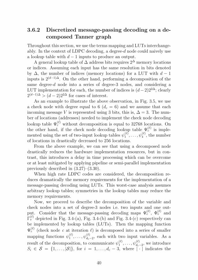
3.4 Decomposition of the variable node and check node into aset of two-input mapping functions (or two-input lookuptables). (a) Check node update operation. (b) Variablenode update operation. (c) Hard decision operation on thevariable node. (d) Decomposition of the check node update
operation Ψ(`)c into the set of two-input mapping functions
ψ(`)1 , . . . , ψ
(`)dc−2. (e) Decomposition of the variable node up-
date operation Φ(`)v into the set of two-input mapping func-
tions φ(`)1 , . . . , φ
(`)dv−1. (f) Decomposition of the hard decision
operation Γ(`)v into the set of two-input mapping functions
This example consider a check node with degree dc = 6 andincoming messages V with a resolution of ∆ = 3 bits. . . . 41
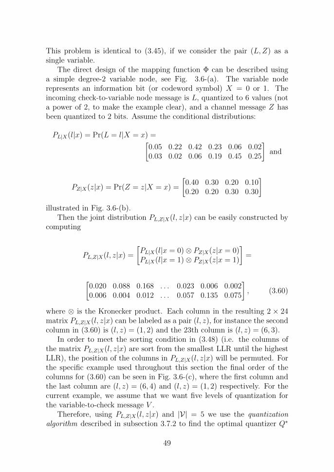
3.6 Overview of the designing process for the mapping func-tion Φ. (a) degree-2 LDPC variable node with inputs Land Z and output V . (b) Input distributions Pr(L|X)and Pr(Z|X). (c) Joint distribution Pr(L,Z|X) quantizedto five-valued variable V using the optimal quantizer Q∗
which maximizes the mutual information between X andV . (d) The resulting lookup table corresponding to Q∗.This lookup table computes V = Φ(L,Z) to maximize mu-tual information. . . . . . . . . . . . . . . . . . . . . . . . 48
4.1 Evolution of the Gaussian pdfs for the variable-to-checkmessage V
(`)j→i. Different values of Eb/N0 are used. . . . . . 55
4.2 Behavior of the mean µ(`) as a function of the number ofiterations `. . . . . . . . . . . . . . . . . . . . . . . . . . . 56
4.3 Noise decoding thresholds for a regular (3, 6)-LDPC codewith rate 1/2 and using different number of levels K forthe decoder message quantization. The term log2(K) isthe number of bits to represent the decoder messages whilelog2(|Z|) is the number of bits to represent the BI-AWGNCmessage. . . . . . . . . . . . . . . . . . . . . . . . . . . . . 64
xvii
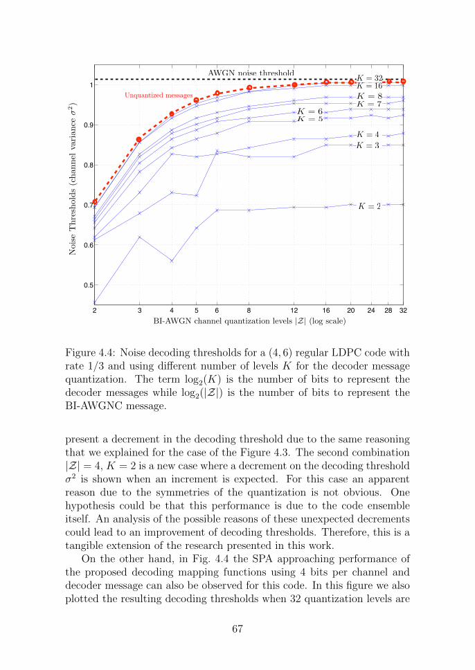
4.4 Noise decoding thresholds for a (4, 6) regular LDPC codewith rate 1/3 and using different number of levels K forthe decoder message quantization. The term log2(K) isthe number of bits to represent the decoder messages whilelog2(|Z|) is the number of bits to represent the BI-AWGNCmessage. . . . . . . . . . . . . . . . . . . . . . . . . . . . . 67
4.5 Tree representation of the implementation of a hard deci-sion operation using lookup table. The node has six inputsincluding the channel message. . . . . . . . . . . . . . . . . 69
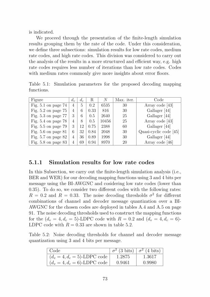
5.1 BER and WER results for the proposed decoding mappingfunctions, and sum-product algorithm. Parameters of thecode: dv = 4, dc = 5, R = 0.2, and N = 6535. The maxi-mum number of Iterations was set to 25. The numbers nextto the curves represent the average number of iterations foreach simulation point. . . . . . . . . . . . . . . . . . . . . 74
5.2 BER and WER results for the proposed decoding mappingfunctions, and sum-product algorithm. Parameters of thecode: dv = 4, dc = 6, R = 0.33, and N = 816. The maxi-mum number of Iterations was set to 25. The numbers nextto the curves represent the average number of iterations foreach simulation point. . . . . . . . . . . . . . . . . . . . . 75
5.3 BER and WER results for the proposed decoding mappingfunctions, and sum-product algorithm. Parameters of thecode: dv = 3, dc = 6, R = 0.5, and N = 2640. The maxi-mum number of Iterations was set to 25. The numbers nextto the curves represent the average number of iterations foreach simulation point. . . . . . . . . . . . . . . . . . . . . 77
5.4 BER results for the proposed decoding mapping functions,and sum-product algorithm. Parameters of the code: dv =4, dc = 8, R = 0.5, and N = 10456. The maximum num-ber of Iterations was set to 30. The numbers next to thecurves represent the average number of iterations for eachsimulation point. . . . . . . . . . . . . . . . . . . . . . . . 78
5.5 Word-error rate results for SPA using floating point num-bers, FAIDs using 7 levels of quantization and the decod-ing mappings (max-LUT ) using 3 and 4 bits per message.A regular (dv = 3, dc = 12)-LDPC code was used withR = 0.75, block length N = 2388 and a maximum of 60iterations. . . . . . . . . . . . . . . . . . . . . . . . . . . . 79
xviii
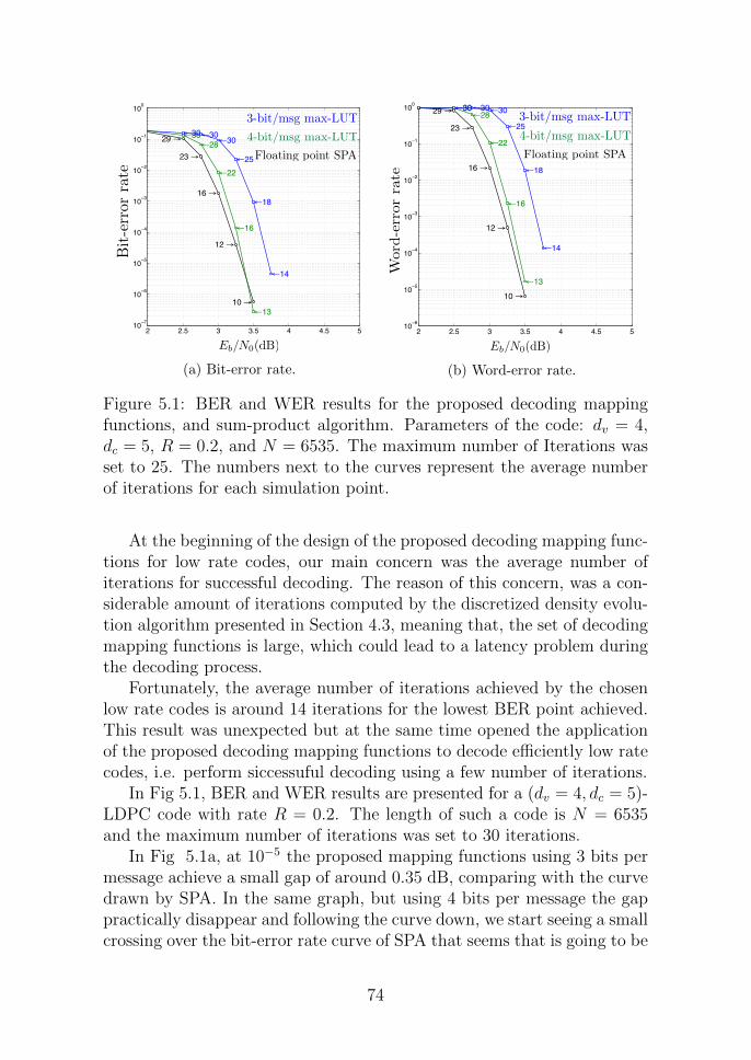
5.6 BER and WER results for the proposed decoding mappingfunctions, and sum-product algorithm. Parameters of thecode: dv = 6, dc = 32, R = 0.84, and N = 2048. The maxi-mum number of Iterations was set to 30. The numbers nextto the curves represent the average number of iterations foreach simulation point. . . . . . . . . . . . . . . . . . . . . 81
5.7 BER and WER results for the proposed decoding mappingfunctions, and sum-product algorithm. Parameters of thecode: dv = 4, dc = 36, R = 0.89, and N = 1998. The maxi-mum number of Iterations was set to 30. The numbers nextto the curves represent the average number of iterations foreach simulation point. . . . . . . . . . . . . . . . . . . . . 82
5.8 BER and WER results for the proposed decoding mappingfunctions, and sum-product algorithm. Parameters of thecode: dv = 4, dc = 69, R = 0.94, and N = 8970. The maxi-mum number of Iterations was set to 20. The numbers nextto the curves represent the average number of iterations foreach simulation point. . . . . . . . . . . . . . . . . . . . . 83
xix
List of Tables
1.1 List of various proposed discrete message-passing decodingalgorithms using a certain number of bits to represent eachreceived coded bit beloging to a received noisy codeword.PLR: Parity likelihood ratio, MS: min-sum, NQBPA: non-uniform quantized belief propagation algorithm, SPA: sum-product algorithm, OMS: offset min-sum, FAID: Finite al-phabet iterative decoder, MD: mapping decoder, max-LUT:lookup table that maximizes mutual information, BSC: Bi-nary symmetric channel, BI-AWGNC: Binary-input addi-tive white Gaussian noise channel. . . . . . . . . . . . . . . 9
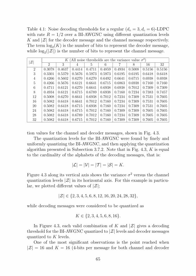
4.1 Noise decoding thresholds for a regular (dv = 3, dc = 6)-LDPC with rate R = 1/2 over a BI-AWGNC using differ-ent quantization levels K and |Z| for the decoder messageand the channel message respectively. The term log2(K) isthe number of bits to represent the decoder message, whilelog2(|Z|) is the number of bits to represent the channelmessage. . . . . . . . . . . . . . . . . . . . . . . . . . . . . 65
4.2 Comparison for different arrangements (trees) to implementa hard decision operation with six inputs including thechannel message. The decoding thresholds σ∗ were com-puted considering that the incoming messages have a reso-lution of 3 bits. . . . . . . . . . . . . . . . . . . . . . . . . 69
5.2 Noise decoding thresholds for channel and decoder messagequantization using 3 and 4 bits per message. . . . . . . . . 73
xx
5.3 Noise decoding thresholds for channel and decoder messagequantization using 3 and 4 bits per message. In the case ofthe (dv = 3, dc = 12)-LDPC code, its variance noise thresh-olds σ2 were used to calculate the corresponding crossoverprobabilities ε for the BSC via the Q-function. . . . . . . . 76
5.4 Decoding thresholds for channel and decoder message quan-tization using 3 and 4 bits per message. . . . . . . . . . . . 80
A.1 Noise decoding thresholds for a regular (dv = 2, dc = 40)-LDPC with rate R = 19/20 over a BI-AWGNC using differ-ent quantization levels K and |Z| for the decoder messageand the channel message respectively. The term log2(K) isthe number of bits to represent the decoder message, whilelog2(|Z|) is the number of bits to represent the channelmessage. . . . . . . . . . . . . . . . . . . . . . . . . . . . . 89
A.2 Noise decoding thresholds for a regular (dv = 3, dc = 4)-LDPC with rate R = 1/4 over a BI-AWGNC using differ-ent quantization levels K and |Z| for the decoder messageand the channel message respectively. The term log2(K) isthe number of bits to represent the decoder message, whilelog2(|Z|) is the number of bits to represent the channelmessage. . . . . . . . . . . . . . . . . . . . . . . . . . . . . 89
A.3 Noise decoding thresholds for a regular (dv = 3, dc = 6)-LDPC with rate R = 1/2 over a BI-AWGNC using differ-ent quantization levels K and |Z| for the decoder messageand the channel message respectively. The term log2(K) isthe number of bits to represent the decoder message, whilelog2(|Z|) is the number of bits to represent the channelmessage. . . . . . . . . . . . . . . . . . . . . . . . . . . . . 90
A.4 Noise decoding thresholds for a regular (dv = 4, dc = 5)-LDPC with rate R = 1/5 over a BI-AWGNC using differ-ent quantization levels K and |Z| for the decoder messageand the channel message respectively. The term log2(K) isthe number of bits to represent the decoder message, whilelog2(|Z|) is the number of bits to represent the channelmessage. . . . . . . . . . . . . . . . . . . . . . . . . . . . . 90
xxi
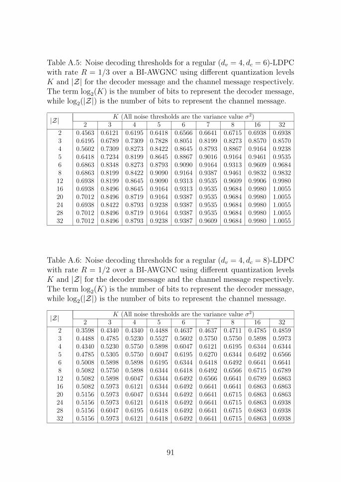
A.5 Noise decoding thresholds for a regular (dv = 4, dc = 6)-LDPC with rate R = 1/3 over a BI-AWGNC using differ-ent quantization levels K and |Z| for the decoder messageand the channel message respectively. The term log2(K) isthe number of bits to represent the decoder message, whilelog2(|Z|) is the number of bits to represent the channelmessage. . . . . . . . . . . . . . . . . . . . . . . . . . . . . 91
A.6 Noise decoding thresholds for a regular (dv = 4, dc = 8)-LDPC with rate R = 1/2 over a BI-AWGNC using differ-ent quantization levels K and |Z| for the decoder messageand the channel message respectively. The term log2(K) isthe number of bits to represent the decoder message, whilelog2(|Z|) is the number of bits to represent the channelmessage. . . . . . . . . . . . . . . . . . . . . . . . . . . . . 91
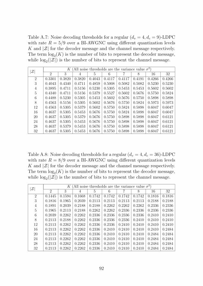
A.7 Noise decoding thresholds for a regular (dv = 4, dc = 9)-LDPC with rate R = 5/9 over a BI-AWGNC using differ-ent quantization levels K and |Z| for the decoder messageand the channel message respectively. The term log2(K) isthe number of bits to represent the decoder message, whilelog2(|Z|) is the number of bits to represent the channelmessage. . . . . . . . . . . . . . . . . . . . . . . . . . . . . 92
A.8 Noise decoding thresholds for a regular (dv = 4, dc = 36)-LDPC with rate R = 8/9 over a BI-AWGNC using differ-ent quantization levels K and |Z| for the decoder messageand the channel message respectively. The term log2(K) isthe number of bits to represent the decoder message, whilelog2(|Z|) is the number of bits to represent the channelmessage. . . . . . . . . . . . . . . . . . . . . . . . . . . . . 92
A.9 Noise decoding thresholds for a regular (dv = 4, dc = 42)-LDPC with rate R = 19/21 over a BI-AWGNC using differ-ent quantization levels K and |Z| for the decoder messageand the channel message respectively. The term log2(K) isthe number of bits to represent the decoder message, whilelog2(|Z|) is the number of bits to represent the channelmessage. . . . . . . . . . . . . . . . . . . . . . . . . . . . . 93
xxii
A.10 Noise decoding thresholds for a regular (dv = 4, dc = 69)-LDPC with rate R = 65/69 over a BI-AWGNC using differ-ent quantization levels K and |Z| for the decoder messageand the channel message respectively. The term log2(K) isthe number of bits to represent the decoder message, whilelog2(|Z|) is the number of bits to represent the channelmessage. . . . . . . . . . . . . . . . . . . . . . . . . . . . . 93
A.11 Noise decoding thresholds for a regular (dv = 6, dc = 32)-LDPC with rate R = 13/16 over a BI-AWGNC using differ-ent quantization levels K and |Z| for the decoder messageand the channel message respectively. The term log2(K) isthe number of bits to represent the decoder message, whilelog2(|Z|) is the number of bits to represent the channelmessage. . . . . . . . . . . . . . . . . . . . . . . . . . . . . 94
xxiii
Chapter 1
Introduction
Source coding and channel coding were initially presented in A Mathemat-ical Theory of Communications [1], the groundbreaking paper publishedby Shannon in 1948. In this paper, Shannon defined channel capacity andproved that it is the upper bound of the rate at which we can transmit in-formation over a noisy channel with a probability of error negligibly small.In the following years a variety of codes were proposed. However, it wasnot until 1993 when turbo codes were published [2], the first class of codesreporting a performance close to the channel capacity. Later, around 1996a rediscovery of low-density parity-check (LDPC) codes were also shownto have near-capacity performance, even though LDPC codes (sometimescalled Gallager codes) were conceived by Gallager in 1961 [3], they weremainly forgotten due to the complexity involved in their implementation.Turbo codes lead themselves to a passionate study but they are outsidethe scope of this work, this work is completely related to the decoding ofLDPC codes.
1.1 Transmission and storage of data
Digital communication and storage systems helping people to share andsave their information can be seen everywhere at anytime. Some of themost common examples of digital communication systems include smartphones, tablets, smart digital television via satellite or cable, internetaccess either wired via cable modem and wirelessly via Wi-Fi and WiMax.On the side of digital storage systems, we can mention optical disk drives(e.g. CD, DVD, Blue-ray), solid-state drives (SSD), memory cards, USBflash drives, and magnetic disk drives, although the latter is increasinglydisappearing from personal devices.
1
Information Source
Compression (Source
encoder)Encryption
Encoding (Channel encoder)
Modulation
Destination Source Decoder Decryption
Decoding (Channel decoder)
Demodulation
ChannelReceiver
Transmitter
Figure 1.1: Block diagram of general digital communication system.
All the above examples of communication and storage systems can bemore globally put into a simple and common framework. Such frameworkwas first proposed by Shannon in [1].
Originally, the block diagram proposed by Shannon of a general com-munication system had five blocks; an information source, transmitter,channel, receiver and destination, see Fig. 1.1. Each of the blocks is de-scribed below. Given that some of the blocks in the diagram perform morethan one operation, those are decomposed and described as a set of welldefined operations.
1. The information source is considered a stream of random numbers(commonly binary) that follow a probability distribution and repre-sent some type of data that a user (a person or a system) wants tocommunicate to other user. The incoming signal to the informationsource block may be digital (e.g. computer file) or analog (e.g., lightbeing sensed by a digital camera, sound capture by a microphone,etc.), in such a case, an analog-to-digital conversion is applied toproduce a digitized output signal.
2. The transmitter is a compound of the following four operations.Since Shannon refers to these operations as a whole, they are drawninside of the transmitter block, see Fig. 1.1.
• Compression (or source coding) can be seen as the operationin the communication process, where the existing redundancy
2
in the user data is eliminated, thus the output of this operationproduces equiprobable outputs. Depend upon the application,the compression can be lossless (lower bounded by the entropyof the data source) or lossy (governed by the rate-distortiontheorem [4, p. 301]).
• Encryption is sometimes considered in the communication sys-tem, and it can be described as a mapping from user data intoa “secret” code, so that non authorized users cannot recognizerelevant data.
• Encoding (or channel coding) is an addition method of struc-tured redundancy to enable error detection/correction capa-bility. Commonly, every incoming sequence of Kcode symbols,called message, is mapped to another sequence of N symbols,called codeword, always having N > Kcode. The ratio Kcode/Nis called code rate and is normally denoted by R such that0 < R = Kcode/N < 1.
• Modulation takes the codewords which have some useful andefficient redundancy and generates the waveforms that meetthe requirements of the specified noisy channel.
3. The channel is the physical medium whereby the modulated out-put is conveyed “through space when signaling from here to there(transmission), or through time when signaling from now to then(storage)” (Hamming [5, p. 20]).
4. The receiver is the counterpart of the transmitter block. There-fore, it is also decomposed into the corresponding “inverse” set ofoperations for those in the transmitter block. These operations arewrapped inside of the receiver block, see Fig. 1.1.
• The demodulation is the part of the receiver in a communica-tion system where the output from the channel is converted intonoisy sequences (other important operations are performed inthis sub block, but they fall beyond the scope of this disserta-tion).
• The channel decoder attempts to recover the original data en-coded by the channel encoder, starting from the demodulatednoisy sequences (or corrupted codewords). It produces validmessages for the following processes wrapped in the receiverside. This is the main subject of this dissertation.
Figure 1.2: Graphical representation of a parity-check matrix H by aTanner graph. Edges interconnecting nodes of different types are drawnwherever there is a one in the matrix H.
• Decryption. Removes any encryption.
• The source decoder recovers the compressed data.
5. The destination represents the user for whom data is intended.
1.2 LDPC codes and their key properties
An LDPC code is a block code for channel coding that has a parity-checkmatrix H which is sparse. There are two types of LDPC codes: regu-lar and irregular. Regular LDPC codes have a constant number of onesdv in each column (column weight) and a constant number of ones dcin each row (row weight), otherwise the code is defined as an irregularLDPC code. LDPC codes can be analysed using a Tanner graph, whichis a bipartite graph that separates the nodes into variable nodes (graph-ically represented by circles corresponding to columns of H) and checknodes (graphically represented by squares corresponding to rows of H),see Fig 1.2 for an example of a parity-check matrix H with dv = 2, dc = 4whose Tanner graph is also shown.
The following results are provided by Gallager [3] and Mackay [6].LDPC codes have a quite simple construction (randomly generated paritycheck matrix), given an optimal decoder, LDPC codes are good codes(code families that achieve arbitrary small probability of error at non-zero communication rates up to some maximum rate that may be lessthan the capacity of a given channel), and they have good distance (theminimum distance dmin of the code divided by the length N of that such
4
code tends to a constant greater than zero). These results hold for anycolumn weight dv ≥ 3. Furthermore, there are sequences of LDPC codesin which dv increases gradually with the length N of the code, in sucha way that the ratio dv/N still goes to zero, this property gives a gooddistance [6, p. 557].
1.3 Decoding of LDPC codes
Using the Tanner graph of an LDPC code, a cycle is defined as a sequenceof edges that form a closed path. For instance, in Fig 1.2 we can observea cycle whose length is equal to the number of edges that form it, forthis specific example such length is equal to 6 and as a result this cycle isdenoted as 6-cycle. If an LDPC code is drawn as a tree (which is possibleonly if there are no cycles in the Tanner graph or in the parity-checkmatrix), optimal message-passing decoding can be achieved, unfortunatelyat the same time, LDPC codes with good minimum distance propertiescannot be found for this setting [7, p. 64]. On the other hand, the existenceof cycles leads to a suboptimal iterative message-passing decoding whichrequires a large length (e.g. 107) to have a probability of error negligiblysmall [8].
The best iterative message passing decoding algorithm known for LDPCcodes is the sum-product algorithm (SPA) (from now on, we will some-times omit the word “iterative” when we refer to decoding algorithms forLDPC codes, since it is understood that the decoding process is iterative),also known as iterative probabilistic decoding or belief propagation (BP).
It is well known that the best decoding performance of LDPC codescan be achieved using the SPA with irregular LDPC codes [9]. In irregularLDPC codes the degree distributions of the nodes are optimized causingnodes with different degrees. However, that increases the complexity ofthe hardware implementation for LDPC decoders. Another problem ofemploying irregular LDPC codes is that the optimal degree distributionsin the nodes generates 4-cyles which generates a decrement in the decodingperformance by causing an abrupt change in the slope of the resulting errorprobability curve, this phenomenon is called the “error floor” [10, p. 399].In contrast, despite regular LDPC codes having an error-rate performancepenalty respect to that achieved by irregular LDPC codes, they providean easy way to design an efficient hardware implmentation of LDPC de-coders due to their structure (i.e. constant dc and dv in rows and columnsrespectively). In this work, we only use regular LDPC codes due to theirfriendly design (e.g. regular LDPC codes based on array codes, shortened
5
array codes, finite geometries, etc.) and hardware implementation (e.g.generic node operations due to constant degree of the nodes, fully paral-lel, serial or hybrid manageable architectures that reduce the integratedcircuit (IC) resources and speed up the throughput of the LDPC decoderwhich allows a scalable design [11]).
1.4 Discrete LDPC decoding algorithms
Although it was mentioned above that the SPA provides the best decodingperformance (i.e. error-rate probability close to the the channel capacity),when it comes to its hardware implementation, it becomes a problem dueto the fact that this algorithm employs nonlinear functions that need ahigh resolution (i.e. 12 or more bits [12]) to represent each coded bit ina codeword. This issue also requires that the corresponding architecturework with high resolution variables that at the same time demand thenecessary arithmetical and logical units to process them.
Depending of the number of bits (resolution) utilized by a definedvariable to represent a coded bit at the decoder, we can define two typesof decoding: hard-decision, when one bit per coded bit is used, and soft-decoding, when high number of bits e.g. 64 bits are used to represent eachcoded bit. Commonly such variables receive the name of messages. There-fore, 4-bit per message means that each variable that represents a codedbit has a resolution of 4 bits which gives 16 possible values to representand processing a given noisy coded bit at the designed message-passingdecoder, e.g. the SPA. As one might expect, the error-rate probabil-ity improves as the number of bits per message increases, for example,soft-decision (more than one bit) gives better decoding performance thanhard-decision (one bit). As a result, the latency for reading and process-ing the messages in an LDPC decoder is proportional to number of bitsper message used to represent such messages. Thus, the target of discreteLDPC decoding algorithms is to reduce the number of bits as much aspossible to reduce the latency of the decoding process. The problem isthat at the same time, for the quantization of LDPC decoding algorithms,a reduction of the number of bits per message can lead to a performancepenalty [3], [13], [14]. Indeed, this topic has received substantial attentionin both the research and engineering communities. Past work on discretemessage-passing decoding algorithms is summarized below.
One of the first works about the implications related to quantizationof the SPA was carried out by Li Ping et al. [12], in this work, it isshown that a quantized SPA using 12 bits per message achieves error-rate
6
performance close to that obtained by SPA without quantization, but stillusing 12 bits per message an error floor is observed. In [12], a binary-input additive white Gaussian noise channel (BI-AWGNC) is considered.To overcome the problem of quantization of the SPA, in [12] a paritylikelihood ratio (PLR) technique is proposed. In [12], using 6 bits permessage an error-rate performance close to non-quantized SPA is shown.
Due to the complex operations involved in the SPA (or BP) to gen-erate the check-to-variable node messages, SPA is usually implementedusing approximations. One of the most common is the so-called BP-basedapproximation [15] (commonly known as the “min-sum” (MS) approxi-mation [16]). Thus, in [17] Chen et al. proposes two BP-based decodingalgorithms to reduce the decoding complexity. Using 6 bits per messagea gap of around 0.1 dB respect to full SPA (without quantization) on theBI-AWGNC is presented.
MS decoding reduces the implementation complexity of the iterativedecoding process performing just a few tenths of a decibel inferior toBP performance. In [18] Zhao et al. study the effects of clipping andquantization on the performance of MS over a BI-AWGNC. The besterror-rate performance is achieved using 6-bits per message with a gap ofaround 0.1 dB respect to that achieved by full SPA.
Chen et al. in [19] reported results using 5, 6 and 7 bits per messagewith an uniform quantization scheme. In this work, using 6 bits per mes-sage on a BI-AWGNC the proposed message-passing decoding algorithmshows error-rate performance identical to full SPA.
In [20] Lee et al. proposed the idea of designing message-passing de-coding algorithms using maximization of mutual information. They useda nonuniform quantization scheme for a regular (dv = 3, dc = 6)-LDPCcode. Comparing with floating point SPA on a BI-AWGNC, 0.2 dB and0.1 dB gaps are observed using 3 and 4 bits per message respectively,albeit a significant amount of hand-optimization is mentioned and theoptimization procedures were not explained in detail.
From an engineering perspective, error floors of the (2048, 1723) Reed-Solomon based LDPC (RS-LDPC) code and (2209,1978) array-based LDPCcode on a BI-AWGNC are studied in [21] by Z. Zhang et al. In it, 6-bituniform quantization is employed for a SPA decoder using a parallel-serialdecoder architecture in a field programmable gate array (FPGA). Part ofthose 6 bits control the range of the quantization (lower negative realvalue and upper positive real value), while the remaining bits define theresolution (quantization step), a parallel-serial decoder architecture in afield programmable gate array (FPGA) was used.
7
Offset min-sum (OMS) over a binary symmetric channel (BSC) using4 bits per message and OMS over a BI-AWGNC using 5 and 6 bits permessage were proposed in [22] by X. Zhang et al.. In this work, using4 bits per message on the BSC is enough to produce identical error-rateperformance than that obtained by OMS without quantization. On theother hand, using 6 bits per message is sufficient to achieve the error-rateperformance of the full OMS over the BI-AWGNC.
More recently, in [23] Planjery et al. propose a 3-bit finite alpha-bet iterative decoder (FAID). FAIDs are designed using the knowledge ofpotentially harmful subgraphs that could be present in a given code. Pre-sented results focus on column-weight-three codes over the (BSC), and inall cases FAIDs decoding performance is better than that obtained by fullSPA.
Lewandowsky et al. also applied the information bottleneck methodto the implementation of quantization in LDPC decoders [24]. Using 4bits per message over a BI-AWGNC, a gap around 0.2 dB respect to theerror-rate performance of full SPA is shown.
In this work we employ binary phase-shift keying (BPSK) modulationsince all the aforementioned work also implemented it in all the simulationsresults. Thus a fair comparison can be made with all the above proposeddiscrete LDPC decoding algorithms.
In Table 1.1, simulation parameters such as type of quantization, gapwith respect to full SPA (if available), number of bits per message, max-imum number of iterations, type of considered channel, as well as otherdetails to identify and analyze each of the above discrete LDPC decodingalgorithms are described. Also the details about the proposed decodingmapping functions for decoding LDPC codes denoted as “This work” arepresented.
In the following section, the idea behind the proposed decoding map-ping functions and their benefits compared with the above described dis-crete LDPC decoding algorithms are delineated.
1.5 Proposed technique for LDPC decoding
In this work, we propose a method to find message-passing decoding map-ping functions for regular LDPC codes which can surpass the error-ratedecoding performance of sum-product algorithm (or BP) using only 4 bitsper message. These results are shown on the BSC and in the BI-AWGNC.From the algorithms listed in Table 1.1 only FAIDs using 3 bits per mes-sage have presented similar results, but only for the BSC.
8
Tab
le1.
1:L
ist
ofva
riou
spro
pos
eddis
cret
em
essa
ge-p
assi
ng
dec
odin
gal
gori
thm
susi
ng
ace
rtai
nnum
ber
ofbit
sto
repre
sent
each
rece
ived
coded
bit
bel
ogin
gto
are
ceiv
ednoi
syco
dew
ord.
PL
R:
Par
ity
like
lihood
rati
o,M
S:
min
-sum
,N
QB
PA
:non
-unif
orm
quan
tize
db
elie
fpro
pag
atio
nal
gori
thm
,SP
A:
sum
-pro
duct
algo
rith
m,O
MS:off
set
min
-sum
,FA
ID:F
init
eal
phab
etit
erat
ive
dec
oder
,M
D:m
appin
gdec
oder
,m
ax-
LU
T:lo
okup
table
that
max
imiz
esm
utu
alin
form
atio
n,
BSC
:B
inar
ysy
mm
etri
cch
annel
,B
I-A
WG
NC
:B
inar
y-i
nput
addit
ive
whit
eG
auss
ian
noi
sech
annel
.
No.
Auth
orA
lgor
ithm
Quan
tiza
tion
Gap
resp
ect
toSP
AN
o.of
bit
sM
ax.
no.
ofit
erat
ions
Chan
nel
IP
ing
etal
.(2
000)
[12]
PL
RU
nif
orm
0.05
640
BI-
AW
GN
CII
Chen
etal
.(2
002)
[17]
BP
-bas
edU
nif
orm
0.1
dB
610
0B
I-A
WG
NC
III
Zhao
etal
.(2
005)
[18]
MS
Unif
orm
0.1
dB
5–6
200
BI-
AW
GN
CIV
Chen
etal
.(2
005)
[19]
MS
Unif
orm
Iden
tica
l6
30B
I-A
WG
NC
VL
eeet
al.
(200
5)[2
0]N
QB
PA
Non
-unif
orm
0.1
dB
3–4
Not
men
tion
edB
I-A
WG
NC
VI
Z.
Zhan
get
al.
(200
9)[2
1]SP
AU
nif
orm
non
e6
200
BI-
AW
GN
CV
IIX
.Z
han
get
al.
(201
2)[2
2]O
MS
Quas
i-unif
orm
Iden
tica
l(O
MS)
4&
5–6
200
BSC
/BI-
AW
GN
CV
III
Pla
nje
ryet
al.
(201
3)[2
3]FA
IDU
nif
orm
Bet
ter
310
0B
SC
IXL
ewan
dow
sky
etal
.(2
016)
[24]
MD
Non
-unif
orm
0.2
dB
450
BI-
AW
GN
CT
his
work
max
-LU
TN
on-u
nif
orm
Bet
ter
3–4
25(a
vera
ge10
–15)
BSC
/BI-
AW
GN
C
9
More precisely, the proposed technique is a systematic method whichuses an optimal quantizer at each step of density evolution to generatemessage-passing decoding mappings which maximize mutual information.Previously in [20] the maximization of mutual information was utilizedto design decoding mapping functions too, but the technique was limitedonly to a specific code rate. On the other hand, in this work the proposedtechnique allows different LDPC codes and as a consequence different coderates which makes the proposed maps suitable for different applications.
FAIDs along with the mapping decoder proposed in [24] by Lewan-dowsky et al., represent the most similar works on the design of decodingmapping functions. Compare with FAIDs, the proposed technique usesan optimal quantizer to construct the decoding mapping functions whileFAIDs use the information of trapping sets existing in the codes. In secondplace, comparing with row IX in Table 1.1, they proposed to use the infor-mation bottleneck method to design the mapping functions, even thoughthey use a discretized density evolution algorithm they have to carry outan extensive search for a good set of mapping functions to decode a speci-fied code. In this work instead of using the information bottleneck method,we use systematically an optimal quantizer. In our case, we can determinea theoretical threshold for a specified LDPC code which is the designedparameter to construct the decoding mapping functions, in this way, weavoid an extensive search for a good set of decoding mapping functions.
The resulting message-passing decoding mappings are not quantizedversions of the sum-product algorithm, or min-sum decoding algorithmnor modifications of these algorithms as in I, II, III, IV, VI and VII inTable 1.1, instead, the proposed maps are based on an optimal quantizerwhich maximizes mutual information [25].
Although the proposed mapping functions achieve near-SPA error-rateperformance using 4 bits per message, it is possible to construct them foran arbitrary number of bits per message, as an example of this, in Chapter5 also results using 3 bits per message are shown.
Our approach has both theoretical and practical aspects. The theo-retical approach of this work is derived from a strong connection betweenthe problem of classification in statistical learning theory, and the prob-lem of optimal quantization of discrete memoryless channels (DMC) ininformation theory. On the practical side, finite-length results for variousregular LDPC code rates show that using 4 bits per message is sufficient toperform close to theoretical limits, achieving or surpassing the error-rateperformance of full SPA.
The proposed maps do not necessarily correspond to elementary math-
10
ematical operations, but may be implemented by a lookup table (LUT).This can lead to a hardware implementation of an LDPC decoder withhigh throughput (number of decoded bits per second). Another signifi-cant benefit of the proposed decoding mapping functions towards a highthroughput LDPC decoder, is that the required number of maximum num-ber of iterations is the lowest among all listed algorithms in Table 1.1,even better, in average the number of required iterations decreases to 10–15 depending of code rate. Added to this, benefits of using a few bitsper message (3 or 4) include: reduction of the memory needed to storethe messages generated along the message-passing decoding process, re-duction in the number of interconnect wires utilized between variable andcheck nodes, reduced complexity of interconnect routing and reduced logiccomplexity [20].
1.6 Summary of contributions
Throughout this work, we aim to describe how to design decoding map-ping functions to decode regular (dv, dc)-LDPC codes which can be im-plemented in integrated circuits using very-large-scale integration (VLSI).For LDPC decoding, the goal is to design decoding algorithms able to meetthree features: 1) error-rate performance close to that of SPA (robust de-coding algorithm able to work in different channels), 2) high throughput(a few bits per message and a few number of iterations) and 3) low gatecount (a few resources for hardware implemntation). The problem is thatnormally if a decoding algorithm achieves 1), it cannot meet 2) and 3) dueto the complexity associated to accomplish 1). On the other hand, if adecoding algorithm meets 2) and 3) it cannot fulfill 1) due to low resolu-tion representation of the variables implicated to estimate valid codewordsduring the decoding process, or due to excessive assumptions that becomethe decoding algorithm efficient for a few particular scenarios.
In this dissertation, a decoding algorithm that meets 1), 2) and 3) ispresented. More precisely, the proposed algorithm is an iterative message-passing decoding algorithm that only uses mapping functions (lookup ta-bles) to perform the local decisions involved in a common LDPC decodingalgorithm (e.g. SPA). The proposed algorithm only performs searches forlookup tables to produce channel messages, decoder messages and estima-tions of valid codewords, that is, the proposed algorithm does not requireany arithmetical operation, instead all messages are positive integers thatare used to search the corresponding value according to the type of nodeand the value of the incoming messages to the node (i.e. the combination
11
of incoming messages represents an address in a lookup table).The proposed algorithm is the result of the combination of previous ac-
complishments that represent the contributions of this dissertation. Suchcontributions are described as follows:
• Max-LUT method. In this research, floating-point algorithms arenot used. Instead, the central method is “direct design” of VLSIfor decoders and channel quantizers. We have developed a tech-nique where the decoder implementation, including quantization ofmessages, are designed using only the probability distribution fromthe channel. Given a probability distribution, our methoddesigns a lookup table (LUT) that maximizes mutual infor-mation, and LUTs are implemented directly in VLSI. Thisis the “max-LUT method”. It is well-known that maximiza-tion of mutual information is Shannon’s channel capacity, and innumerical results so far, the proposed method has excellent quanti-zation/performance tradeoff.
• Quantized density evolution. Since we were interested in pre-dicting the decoding performance of the proposed message-passingdecoding algorithm, we derive a density evolution algorithm that sys-tematically at each step of the density evolution process performsan optimal quantization (optimal in terms of maximizing mutualinformation). The quantized density evolution algorithm that weproposed, allows us to compute the theoretical decoding thresholdfor a regular (dv, dc)-LDPC code ensemble and a specified number ofquantization levels K under the proposed decoding algorithm basedon mapping functions that maximize mutual information.
• Efficient implementation of LDPC decoders. For the design ofLDPC decoders, the max-LUT method is analogous to finding non-uniform quantization schemes where the quantization can vary witheach iteration. In our finite-length results: the proposed decodingmapping functions using 3 bits per message have a gap around 0.4dB with respect to the error-rate performance achieved by full SPA.On the other hand, the proposed decoding mapping functions using4 bits per message are usually sufficient to achieve the error-rateperformance of full SPA. Under the proposed decoding technique,the usual complexity of non-uniform quantization is avoided by usinglookup tables. Lastly, the proposed decoding mapping functionsusing 4 bits per message show lower error floor than full SPA.
12
1.7 Dissertation outline
This dissertation is organized as follows.In Chapter 1, introduction to LDPC codes and their basic properties
as well as their decoding is mentioned. In this chapter also motivation ondiscrete LDPC decoding algorithms is presented. Later, the properties ofthe proposed decoding mapping functions are delineated as well as theirmain results. At the end of the chapter, the summary of the contributionsof this dissertation are described.
In Chapter 2, some fundamental concepts and useful facts about codingtheory are formally described. The framework for the proposed researchis established in this chapter. Fundamentals about LDPC codes and thesum-product algorithm are described in this chapter.
In Chapter 3, we aim to describe the origin of the so-called sum-product algorithm starting from its graphical representation in a tree untilits graphical representation in the so-called Tanner graph. Later in thischapter, we present the max-LUT method and its application to channelquantization and its application to designing local decoding lookup tables.
In Chapter 4, we first introduce the idea behind the density evolutionalgorithm. Later, we describe a discretized density evolution algorithmwhich uses the max-LUT method to systematically perform quantizationon the conditional probability distributions to generate the proposed de-coding mapping functions. We also describe how to compute thresholdsfor a given number of quantization levels K and for a given regular (dv, dc)-LDPC code.
In Chapter 5, we analyze the error-rate performance of the proposeddecoding mapping functions of a wide range of extensive simulation resultsfor finite-length LDPC codes considering the BI-AWGNC and the BSC.
Finally, conclusions, as well as the future work, are presented in Chap-ter 6.
13
Chapter 2
Preliminaries
In this chapter, we firstly establish the conventional performance measuresfor message-passing decoders. Later, we recall the channel capacity and itsapplication for discrete memoryless channels of interest. At the end of thischapter, we formally introduce the matrix and graphical representation ofLDPC codes, to later describe the sum-product algorithm for differentchannel models.
2.1 Performance measures
Automatic request-for-repeat (ARQ) technique and forward error correc-tion (FEC) technique can be seen as the two branches of error-controlcoding. Firstly, ARQ is a technique which aims to carry out the task oferror detection using retransmission requests; in other words, its goal is todetect whether or not a received sequence of symbols (commonly bits) haserrors, which are produced due to transmission through a noisy channel.In the case that an ARQ has detected errors in the received sequence, a re-quest of retransmission of the last sequence is sent to the transmitter fromthe receiver. Secondly, FEC is the scheme whereby existing errors in thereceived sequence (codeword) are corrected applying an error-correctioncode. FEC systems normally target a low probability of decoding error.There are systems which mix both schemes to guarantee reliable trans-missions, an example of this is the IEEE 802.16-2005 standard for mobilebroadband wireless access, also known as “mobile WiMAX”.
Although ARQ techniques are enormously useful, in this work we con-centrate on LDPC decoding which is a FEC technique.
Consider the transmission of the binary codeword u. The bit-errorprobability Pb or sometimes also referred as BER is the probability that
14
the jth estimated bit uj at the channel decoder output is not equal to theencoded bit uj at the channel encoder output, this is,
Pb = Pruj 6= uj. (2.1)
Another performance measure commonly found in coding theory lit-erature is the codeword-error probability, Pcw also referred as word-errorrate (WER) or frame-error rare (FER). Pcw is defined as the probabilitythat the estimated channel decoder codeword u is not equal to the channelencoder codeword u, this is,
Pcw = Pru 6= u. (2.2)
When it comes to compare decoding algorithms, commonly one is ableto see the decoding results as graphs where bit-error rate (BER)/frame-error rate (FER) curves evaluated in a chosen range of signal-to-noise ratio(SNR) are presented. In this work, we shall use the above performancemeasures to present the decoding performance for the proposed decodingalgorithms.
2.2 Channel capacity
Information theory is incredibly relevant for coding theory, it establishesthe “playground” of coding schemes by clearly defining the performancebounds. The most important equation in information theory is the equa-tion to calculate the mutual information between two random variables Xand Y . The mutual information is the average information that one ran-dom variable has about another random variable. Recalling the generalcommunication system model shown in Fig. 1.1, X normally representsthe channel input, while Y represents the channel output. When thesetwo random variables X and Y take values from discrete alphabets X and
15
Y respectively, the mutual information can be found as
I(X;Y ) = H(Y )−H(Y |X) (2.3)
I(X;Y ) =−∑y∈Y
p(y) log2 p(y)−∑x∈X
p(x)H(Y |X = x) (2.4)
I(X;Y ) =−∑y∈Y
p(y) log2 p(y) (2.5)
−∑x∈X
p(x)∑y∈Y
p(y|x) log2 p(y|x) (2.6)
I(X;Y ) =−∑y∈Y
p(y) log2 p(y) (2.7)
−∑x∈X
∑y∈Y
p(x, y) log2 p(y|x), (2.8)
where H(Y ) is the entropy of the channel output Y , and H(Y |X) is con-ditional entropy of Y given X. Mutual information has various proper-ties [4], one of its properties is that it is symmetric in X and Y , suchthat
I(X;Y ) = I(Y ;X) (2.9)
= H(X)−H(X|Y ). (2.10)
The channel capacity C of a discrete memoryless channel (DMC) 1
with input X and output Y is the maximization of mutual informationI(X;Y ), where the maximization is over the channel input probabilitydistribution p(x), resulting in
C = maxp(x)
I(X;Y ). (2.11)
The idea behind the channel capacity C is of wide interest for commu-nication systems because it aims to find the maximum achievable rate Rat which we can reconstruct the channel input sequences (codewords) atthe channel output with a negligible probability of error Pb.
2.3 Channel capacity for useful DMCs
In all practical communication systems, the goal is to transmit data reli-ably through a noisy channel at the maximum possible rate. In order to be
1A channel is said to be memoryless if the probability distribution of the outputdepends only on the input at that time and is conditionally independent of previouschannel inputs or outputs.
16
Cap
acity0
1
0
1
Binary symmetric channel
X Y
1 "
"
1 "
"
"
0 0.1 0.2 0.3 0.4 0.5 0.6 0.7 0.8 0.9 10
0.1
0.2
0.3
0.4
0.5
0.6
0.7
0.8
0.9
1
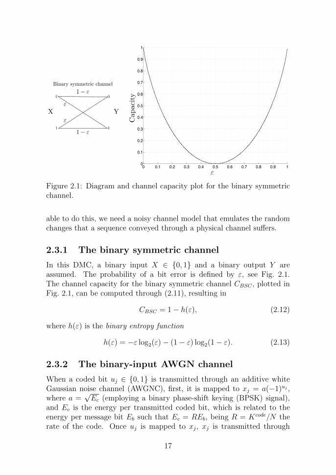
Figure 2.1: Diagram and channel capacity plot for the binary symmetricchannel.
able to do this, we need a noisy channel model that emulates the randomchanges that a sequence conveyed through a physical channel suffers.
2.3.1 The binary symmetric channel
In this DMC, a binary input X ∈ 0, 1 and a binary output Y areassumed. The probability of a bit error is defined by ε, see Fig. 2.1.The channel capacity for the binary symmetric channel CBSC , plotted inFig. 2.1, can be computed through (2.11), resulting in
CBSC = 1− h(ε), (2.12)
where h(ε) is the binary entropy function
h(ε) = −ε log2(ε)− (1− ε) log2(1− ε). (2.13)
2.3.2 The binary-input AWGN channel
When a coded bit uj ∈ 0, 1 is transmitted through an additive whiteGaussian noise channel (AWGNC), first, it is mapped to xj = a(−1)uj ,where a =
√Ec (employing a binary phase-shift keying (BPSK) signal),
and Ec is the energy per transmitted coded bit, which is related to theenergy per message bit Eb such that Ec = REb, being R = Kcode/N therate of the code. Once uj is mapped to xj, xj is transmitted through
17
LDPC encoder
Uncoded bits
“0”“1”
BPSK modulation
xu+
EbDetection
xi =pEc(1)ui
LDPC decoder
y
u
R = Kcode/N
$ N (0,2)
pEc
pEc
Figure 2.2: Block diagram that represents the transmission of a binarycodeword u through the BI-AWGNC. Coding a decoding are assumed tobe carried out by LDPC codes.
a channel which adds a Gaussian noise value $j with zero mean andvariance σ2 = N0/2, i.e., $j ∼ N (0, σ2). At the output of the channelthe real value yj ∈ R, being yj = xj + $j is received. Therefore, thischannel is known as the binary-input AWGN channel (BI-AWGNC). Thetransmission of the binary codeword u through the BI-AWGNC is shownin Fig 2.2, where coding and decoding are assumed to be performed usingLDPC codes.
The capacity of the BI-AWGNC is
CBI−AWGNC = 0.5∑x=±a
∫ ∞−∞
p(y|x) log2
(p(y|x)
p(y)
)dy, (2.14)
where
p(y|x = ±a) =1√2πσ
exp[−(y ± a)2/2σ2] (2.15)
and
p(y) =1
2[p(y|x = +a) + p(y|x = −a)]. (2.16)
Following (2.11), we can derive another formula to compute CBI−AWGNC ,this is, C = H(Y )−H(Y |X) = H(Y )−H(Z), whereH(Z) = 0.5 log2(2πeσ2),thus we have
CBI−AWGNC = −∫ ∞−∞
p(y) log2(p(y)) dy − 0.5 log2(2πeσ2). (2.17)
18
Capacity(bits/channelsymbol)
−2 0 2 4 6 8 100
0.1
0.2
0.3
0.4
0.5
0.6
0.7
0.8
0.9
1
S
h
a
n
n
o
n
c
a
p
a
c
i
t
y
Hard-decision
Soft-decision
C=
0
.5l
o
g
2 1
+
1
2
Eb/N0 (dB)
(Binary symmetric channel (BSC))
Figure 2.3: Plotting soft-decision and hard-decision capacity curves forthe BI-AWGNC, along with the curve for the Shannon capacity.
Note that the integral in (2.17) may be estimated as
E− log2(p(y)) ' − 1
J
J∑j=1
log2(p(yj)), (2.18)
where yj : j = 1, . . . , J is a large group of realizations of Y (say 106)and E· indicates the expected value of the discrete random variable.
In Fig. 2.3, the capacity curve CBI−AWGNC (labeled “soft-decision”)versus the (bit) signal-to-noise ratio Eb/N0 in dB is plotted . Recall thatEb/N0 = E[x2
j ]/2Rσ2 (in this work we assume E[x2
j ] = 1 ). The value Rused in the Eb/N0 is considered as R = CBI−AWGNC , because R is assumedto be lower than CBI−AWGNC just by an arbitrary small value δ, this is
In order to compute the hard-decision BI-AWGNC capacity curve (labeled“hard-decision”), the hard-decisions yj from yj must to be obtained asfollows
yj =
1 if yj ≤ 0
0 if yj > 0.(2.20)
19
Note that these hard-decisions transform the BI-AWGNC into a binarysymmetric channel with error probability ε such that, first, we can applythe Q-function2 to estimate ε, resulting in
ε = Q(√
2REb/N0), (2.21)
later recalling (2.12), we write CBSC = 1− h(ε) to finally produce
Eb/N0(dB)hard = 10 log10(1/(2CBSCσ2)). (2.22)
In Fig. 2.3, the Shannon capacity curve is also shown, without loss ofgenerality, this is
Even though we introduced LDPC codes in section 1.2 of Chapter 1, herewe concentrate our attention in the description of the sum-product algo-rithm. Fig. 1.2 is used again but, modified to describe the flow of themessages in the context of message-passing decoding and thus be able toexplain some useful equations of this section.
Due to complexity implementation requirements associated to the LDPCcodes in 1960, these linear block codes were forgotten for a while, until inthe mid 1990s with the work of MacKay, Luby, and others, they came backagain, but this time they continue being an interesting research topic.
The main reason why these codes are frequently studied, is becausethey have shown to have decoding performance close to the Shannon ca-pacity [8].
This section follows the presentation of LDPC codes in [10] and [26]. Inthis research, only binary LDPC codes are considered. The representationof LDPC codes can be carried out either in matrix form or in a graphicalform.
2The Q-function is the probability that a unit Gaussian N ∼ N (0, 1) exceeds x [26]:Qfunc(x) = Pr(N > x) = 1√
2π
∫∞x
exp (−n2/2) dn.
20
2.4.1 Matrix representation
An LDPC code is a linear block code given by the null space of an M ×Nparity-check matrix H, which has a low density of ones. A regular LDPCcode has a constant number of ones dv in each column and a constantnumber of ones dc in each row, otherwise the code is called irregular.Thus, the code rate R of a regular LDPC is
R ≥ 1− M
N= 1− dv
dc(2.25)
with equality when H is full rank. An example of a parity-check matrixis as follows
where M = 5, N = 10, dv = 2 and dc = 4. Looking closely at the paritycheck matrix in (2.26), we can see that the first row is not independent, thisis, it is the addition of the rest four rows. As a result R = 1−4/10 = 3/5.
2.4.2 Graphical representation
To graphically represent a parity-check matrix H of an LDPC code, we usea Tanner graph, which is a bipartite graph, that is, the nodes are separatedinto two types: check nodes, denoted as CN and variables nodes, denotedas VN, with edges connecting only nodes from different types. For eachH there are M check nodes and N variable nodes. The Tanner graphconstruction is as follows: each check node CN i is connected to a VN jwhenever element hi,j of H is equal to 1. Considering the parity-checkmatrix in (2.26), the corresponding Tanner graph is depicted in Fig. 2.4.
Before describing the iterative decoding process of the SPA, we firstneed to define some useful notation. We denote the set of VNs j thatparticipate in the CN i as
N (i) = j : hi,j = 1, (2.27)
in a similar manner, we denote the set of CNs i that participate in theVN j as
M(j) = i : hi,j = 1. (2.28)
21
1 2 3 4 5
6 7 8 9 102 3 4 51
Check nodes
Variable nodes
Vj!i Li!j
Figure 2.4: Tanner graph for the parity-check matrix H in (2.26)
Using (2.27) and our example of a parity check matrix in (2.26), wecan write the set of VNs j that participate in each CN i as follows
We use N (i)\j to indicate the set N (i) without the element j, e.g.,N (1)\3 = 1, 2, 4. Note that in the Tanner graph the messages sent fromVN j to the CN i are denoted as Vj→i, while the messages sent from theCN i to the VN j are denoted as Li→j, this can be observed in Fig. 2.4.
2.5 The Gallager sum-product algorithm
In this section we describe the sum-product algorithm (SPA). At the be-ginning of SPA, we initialize the variable-to-check node messages Vj→i
with the log-likelihood ratio (LLR) as
Lj = L(uj|yj) = log
(Pr (uj = 0|yj)Pr (uj = 1|yj)
), (2.29)
22
whenever hi,j = 1. Below, we define the LLRs for the BSC and for theBI-AWGNC. For the BSC with b ∈ 0, 1 and bc as a complement (i.e.when b = 0, bc = 1 and vice versa), we have
Lj = L(uj|yj) = (−1)yj log
(1− εε
), (2.30)
where the channel output yj ∈ 0, 1 and ε = Pr(yj = bc|uj = b). In thecase of the BI-AWGNC, we have
Lj = L(uj|yj) = 2yj/σ2, (2.31)
being uj ∈ 0, 1, xj = (−1)uj and the channel output yj = xj +$j, wherethe $j are independent and normally distributed as N (0, σ2). Once theLLRs in (2.30) and (2.31) have been defined, the iterative SPA is as follows:
1. Initialization. For all j, initialize Lj according to (2.29) for theappropriate channel model used. Then, for all i, j that hi,j = 1, setVj→i = Lj.
2. Check node update. Compute Li→j for each check node as
Li→j = 2 tanh−1
( ∏j′∈N (i)\j
tanh
(1
2Vj′→i
)), (2.32)
and then transmit to the variable nodes.
3. Variable node update. Compute Vj→i for each variable node as
Vj→i = Lj +∑
i′∈M(j)\i
Li′→j (2.33)
and then transmit to the check nodes.
4. LLR total. For j = 1, 2, . . . , N compute
Ltotalj = Lj +
∑i∈M(j)
Li→j. (2.34)
5. Stoping criteria. For j = 1, 2, . . . , N , set
uj =
1 if Ltotal
j < 0
0 else ,(2.35)
to obtain u. if uHT = 0 or the number of iterations equals themaximum number of iterations, stop; else, go to step 2.
23
The equation (2.32) for the check node update, is the part of the SPAthat increases the complexity of a hardware implementation and at thesame time is quite sensible to quantization, this happends due to the prod-uct, tanh and tanh−1 operations involved. Mainly the complexity issues ofthe equation (2.32) are the motivation of all discrete LDPC decoding algo-rithms shown in Table 1.1 in page 9 on chapter 1, as well as the motivationof this work.
24
2.6 Summary
In this chapter, first we formally describe the bit-error rate and word/frame-error rate as performance measures for decoding algorithms. In chapter5, we will use this measures to analyze the error-rate performance of theproposed decoding mapping functions for regular (dv, dc)-LDPC codes.
Later, we described shortly the channel capacity and we write its cor-responding equation for some discrete memoryless channels that we usein this work.
At the end of the Chapter, we present the sum-product algorithm andwe mentioned that the complexity of the check node update equation(2.32) for its hardware implementation is the motivation of this work andthat of others proposed decoding algorithms.
25
Chapter 3
Max-LUT method:Maximizing mutualinformation
In this chapter, we describe a technique where the factor-graph-baseddecoders and channel quantizer implementations, including quantizationof messages, are designed using only the probability distribution from thechannel. Given a probability distribution, our method designs a lookup ta-ble (LUT) that maximizes mutual information. In addition, LUTs are de-sirable by engineers who design very-large-scale integration (VLSI) hard-ware implementations of the above operations. This method is called the“max-LUT method”.
Before presenting the max-LUT method, we are interested in describ-ing the origin of the sum-product algorithm (SPA) and its variations thatlead to some of its approximations (e.g. min-sum). This is important inthe first place to clarify the difference between the SPA and its approxi-mations with respect to the proposed decoding algorithm. In the secondplace, the description of the origin of SPA will also give a landscape overpossible range of applications that the proposed factor-graph-based decod-ing algorithm could have. Also the decomposition of the local decodingfunctions can be understood by describing the core of the SPA.
3.1 Factorization of a global function
Algorithms that have to deal with marginals of multivariate functions,normally exploit the factorization of the global function. This leads tothe computation of a set of simpler local functions which only receive
26
as arguments a few random variables of the global function. An specificexample of these type of algorithms are the decoding algorithms based ongraphs, e.g sum-product algorithm to decode LDPC codes.
The essential idea of using the product of local functions to solve amarginalize-product-of-functions (MPF) problem was first explicitly pre-sented by Aji and McEliece [27]. Aji and McEliece in [28] proposed ageneralized distributive law which may solve some MPF problems usingjunction trees (i.e. a mapping of a graph into a tree), but more impor-tantly, it can also be used in factor graphs to describe the functionality ofa generic message-passing decoding algorithm commonly called the sum-product algorithm. This result is significant because algorithms developedin digital communications and other disciplines may be derived as a par-ticular case of the sum-product algorithm attached to a suitable factorgraph.
As an example of a global function f and its factorization, consider aset of six binary random variables u1, u2, u3, u4, u5, u6 ∈ 0, 1 such thatf(u1, u2, u3, u4, u5, u6). Suppose, f and its factorization are as follows
For this specific example, the global function f is factorized into fourfactors f1, f2, f3 and f4.
Taking f and its factorizarion, we are interested in a graphical repre-sentation. For this matter, we can draw a factor graph as follows: eachvariable u; in the global function f is represented with a variable node (cir-cle) and each factor of f in (3.1) is represented by a factor node (square).The corresponding factor graph of the example in (3.1) is shown in theleft hand side of Fig. 3.1. Then, using edges connect a variable node toa factor node whenever such variable node is an argument of that factornode, e.g. in Fig. 3.1, we connect the variable nodes u1, u2 and u3 to thefactor node f1.
Note that the factor graph in Fig. 3.1 is in fact a tree with root in u1
for convenience. In this tree edges only connect nodes of different types;in other words, the factor graph of the example in (3.1) is a bipartite treesince it has two types of nodes; variable and factor nodes. As a result,there is only one path between two nodes, e.g. there is only one pathbetween the variable nodes u3 and u5; this is indicated on Fig. 3.1 with adashed line.
The property that a global function can be represented by a bipartitetree (no closed paths) is useful because it leads to the computation of a
27
f1 f2
f3 f4f3
f1
f2
u1
u2 u3 u4
u5
u6
u1
u7
u3
u4
u6
u5
u2 u1 + u2 + u4 = 0
u3 + u4 + u6 = 0
u4 + u5 + u7 = 0
Figure 3.1: Representation of a bipartite tree with two factors (subtrees)closed by ellipses (left hand side). Tanner graph of a code Ccode with itscorresponding check node equations (right hand side).
generic factorization of the global function. This property later will allowthe computation of exact marginals that become the main assumptionbehind the node equations for the sum-product algorithm.
At the beginning of this section, we mentioned that the factorizationof a global function e.g. f , is useful for decoding algorithms, in order toshow the connection, we will use the following example. Consider a binarylinear code Ccode whose parity check matrix is
H =
1 1 0 1 0 0 00 0 1 1 0 1 00 0 0 1 1 0 1
. (3.2)
Therefore, Ccode has a set of binary codewords u of the form u =(u1, u2, u3, u4, u5, u6, u7). In this example, the task of the global functionf is to verify if each incoming binary sequence u is a codeword of Ccode
(in this example f has seven arguments and different factorization thanin (3.1)). Thus, the global function f is
f(u1, u2, u3, u4, u5, u6, u7) =
1, if uHT = 0,
0, otherwise.(3.3)
Using the nonzero elements in each row of the parity check matrix H in(3.2), the global function f can be factorized as
where each factor f1, f2 and f3 of f is equal to 1 if the modulo two addition(i.e. checksum) of its arguments u is equal to 0, otherwise is 0. In otherwords, the global function f is satisfied when f1, f2 and f3 are equal to 1,meaning that the incoming sequence u satisfies uHT = 0. The graphicalrepresentation of the above example receives the name of Tanner graphand is shown in right hand side of Fig. 3.1. Since each factor of f in (3.4)performs checksums, in the literature the factor nodes of the Tanner graphare commonly called check nodes. In this way, we can say that a Tannergraph is a particular case of a factor graph applied to the description ofcodes.
3.2 Recursive determination of marginals
Employing the example in (3.1), suppose that we are interested in com-puting the marginal of the global function f respect to u1, this is,
f(u1) =∑
u2,u3,u4,u5,u6
f(u1, u2, u3, u4, u5, u6)
=∑∼u1
f(u1, u2, u3, u4, u5, u6).(3.5)
Note that we introduce the not-sum or summary denoted as∑∼·
which indicates the variables not being summed over, i.e. the marginal off respect to u1 is the not-sum for u1 of f .
Now, consider a generic global function g whose graphical representa-tion is a bipartite tree. Then, we are interested in computing the marginal
g(r) =∑∼r
g(r, . . . ). (3.6)
In order to reduce the complexity of the marginalization in (3.6), wewill exploit the fact that g can be represented as a tree. Therefore, g hasa generic factorization as follows
29
g(r, . . . ) =W∏w=1
[gw(r, . . . )], (3.7)
where W is an integer. An important property of the factorization in(3.7) is that the variable r is an argument of each factor gw, but all othervariables only appears in one of the factors.
Thus, the factorization in (3.7) applied to the example in (3.1) gives
where W = 2. In a graphical way, the above factorization of f is depictedin Fig 3.1. In this figure the factorization of f in (3.8) is graphically thepartition of the tree into two subtrees with root u1, this is highlighted byellipses closing the two subtrees or factors of f .
Using the generic factorization of the function g in (3.7) and the dis-tributive law, we can rewrite the marginalization of g respect to r asfollows
g(r) =∑∼r
g(r, . . . ) =∑∼r
W∏w=1
[gw(r, . . . )] =W∏w=1
[∑∼r
gw(r, . . . )
]. (3.9)
Note that the marginal∑∼r g(r, . . . ) is the product of individual
marginals∑∼r gw(r, . . . ). Therefore, the application of (3.9) to the
marginalization of f respect to u1 will produce
f(u1) =
[ ∑∼u1
f1(u1, u2, u3)
][ ∑∼u1
f2(u1, u4, u6)f3(u4)f4(u4, u5)
].
(3.10)
Since we want to decompose g in small pieces to perform simper localoperations, we define a generic factorization for each gw which contains akernel and the product of factors, this is,
30
gw(r, . . . ) = η(r, r1, . . . , rJ)︸ ︷︷ ︸Kernel
J∏j=1
[ηj(rj, . . . )
]︸ ︷︷ ︸
Factors
. (3.11)
Thus, the kernel is the function contained in the root node of the currentfactor gw. Note that the above generic factorization of gw only has thevariable r in the kernel while each of the other variables rj appears atmost twice; sometimes in the kernel and in one of the factors ηj(rj, . . . ).Identifying the structure of (3.11) in f , we can write f as
f(u1, u2, u3, u4, u5, u6) = [f1(u1, u2, u3)︸ ︷︷ ︸
Kernel
[1]︸︷︷︸u2
[1]︸︷︷︸u3
]︸ ︷︷ ︸
First factor
·
[f2(u1, u4, u6)︸ ︷︷ ︸
Kernel
[f3(u4)f4(u4, u5)︸ ︷︷ ︸u4
] [1]︸︷︷︸u6
]︸ ︷︷ ︸
Second factor
.
(3.12)
Taking advantage of (3.11), we can compute the marginal∑∼r gw(r, . . . )
by multiplying the kernel η(r, r1, . . . , rJ) with the individual marginals∑∼rj ηj(rj, . . . ) and summing all the remaining variables different than
r, more precisely
∑∼r
gw(r, . . . ) =∑∼r
η(r, r1, . . . , rJ)J∏
j=1
[ ∑∼rj
ηj(rj, . . . )]
(3.13)
At this point we can apply (3.9) and (3.13) to recurvely fragment themarginalization of g respect to r until we reach the leaves of the tree. Notethat the marginalization process is governed by the structure of the tree.
In the following section, we describe the method to compute the marginalsof the global function g whose graphical representation is a bipartite tree,such a method is called message-passing algorithm.
31
3.3 Message-passing algorithm in cycle-free
factor graphs
The message-passing algorithm in cycle-free factor graphs (trees) is amethod that sends messages along the edges of the tree, starting fromthe leaves and ending at the root. These messages are marginals of partof the global function g that at the end are combined to compute themarginal of the global function respect of a given variable r (root).
Assuming a tree with root r (or a rooted cycle-free factor graph in r),the message-passing algorithm is as follows:
1. the calculation begins in the leaf nodes of the tree;
• if the leaf node is a variable node, it sends an identity function(i.e., 1) to its parent node,
• if the leaf node is a factor node, it sends a description of f toits parent node.
2. Each node must to wait to receive all incoming messages from itschildren to compute its outgoing message that will be transmited toits parent;
• if the the node is a variable node, it sends the product of allincoming messages from its children,
• if the the node is a factor node, it performs the product of itsfunction f with all incoming messages from its children, andthen, it applies the summary
∑∼r′ or not-sum of r′, where r′
is its parent.
We have described in two general steps the computation of the marginal-ization of a global function g respect to r, but we are interested in com-puting the marginals for each variable in the global function g.
Computing all marginals of a global function g is possible by apply-ing the previously described message-passing algorithm to different treeswhich have one of the variables of g as a root. On the other hand, a betterapproach is to compute the marginals of each variable of g in the sametree. In order to do that, we start at all leaf nodes and for each node wecompute an outgoing message once we have all other incoming messagesfrom the rest of adjacent edges to the given node. Each node performsthese operations until all edges have transmitted messages in both direc-tions. At the end, each variable node of the tree is able to calculate thecorresponding marginal.
32
The initialization conditions as well as the node operations of themessage-passing algorithm are shown in Fig 3.2. Looking at this figure,note that a considerable amount of operations performed are sums andproducts, carried out along the message-passing algorithm, for this rea-son, sometimes it is called sum-product algorithm.
Since we are interested in the decoding of binary LDPC codes, it isimportant to mention that the function f that appears in the factor nodein Fig 3.2 is the the addition modulo 2 of all its arguments which definea binary sequence. The purpose of this function when decoding binaryLDPC codes is to add all probabilistic products of sequences that haveeven number of ones and on the other side, add all the probabilistic prod-ucts of sequences that have odd number of ones.
Later in section 3.5, we will explain some of the most common parame-trization of the node function that lead to different approaches to performthe message-passing decoding algorithm to decode LDPC codes.
3.4 Message-passing algorithm in factor gra-
phs with cycles
A linear block code Ccode, defined by its parity-check matrix H with Mrows and N columns, can be represented by a factor graph with N vari-ables nodes and M factor nodes. As an example, consider a linear blockcode Ccode whose parity-check matrix is
H =
1 1 0 1 1 0 01 0 1 1 0 1 00 1 1 1 0 0 1
, (3.14)
the corresponding factor graph for the above matrix can be drawn asshown on the left hand side of Fig. 3.3. On the other hand, a more usefuland structured graph is the Tanner graph which is depicted on the righthand side of Fig. 3.3. Although both graphs are graphical representationsof Ccode, normally the Tanner graph is used to analyze the local decodingfunctions involved in the message-passing algorithm. In Fig. 3.3, a closeddashed path is shown, this is called a cycle whose girth is equal to foursince the cycle is constructed by four edges; in the literature this is writtenas a 4-cycle.
The implication of an existing cycle in a parity check matrix impliesthat Ccode cannot be represented by a tree. This further implies that
33
(u) = 1
(u) =QW
w=1 w(u)
(u) =P
u f(u, u1, . . . , uJ)QJ
j=1 j(uj)
QW+1w=1 w(u)
f1 fw fW
fW+1
f1 fw fW
fW+1
1 w W
W+1
u
1 w W
u
u
(u) = f(u)
u
f
f
f
u1 uj uJ
1 j J
Factor node
Variable node
Marginalization
Initialization in the leaf nodes
Figure 3.2: Initialization conditions and node operations of the message-passing algorithm on a bipartite tree.
34
u1 u2
u3
u4
u5
f1 f2f1
u6
f3
f3
f2 u1 u2 u3 u4 u5 u6 u7
u7
Figure 3.3: A factor graph representation of a linear block code (left).Tanner graph representation of a linear block code emphasizing an existing4-cycle by dashed lines (right)
the variable nodes are not statistically independent and as a result themarginals of the message passing decoding are not exact, which leads toa suboptimal decoding.
On the other hand, if a linear block code Ccode of length N has a Tannergraph without cycles, the maximum-likelihood soft-decision decoding ofCcode can be achieved in time O(n2). However, in [29] it has been shownthat cycle-free Tanner graphs cannot support good codes. Specifically, itis proved that if the rate R of a code Ccode is greater than or equal to0.5 the minimum distance dmin is lower than or equal to 2. On the otherhand, if R < 0.5, Ccode is obtained from a code of rate ≥ 0.5 and distance≤ 2 by simply repeating some symbols.
Even though the propagation rules of the sum-product algorithm shownin Fig 3.2 are considered for a cycle-free graphs (trees), they may also beapplied to factor graphs with cycles. Although the results of the message-passing algorithm operating in a factor graph with cycles cannot in generalbe interpreted as exact function summaries, positive results from variousdecoding codes such as turbo codes and low-density parity-check (LDPC)codes have been reported [2], [30], [31].
35
3.5 Message-passing decoding and its vari-
ations
In this section we are interested in the structure of the equations of thesum-product algorithm and their variations. The generic updating rulesof the nodes of a factor graph were shown in Fig 3.2. In this section weare interested is defining the variable node update and the check nodeupdate as two mapping functions Φ and Ψ respectively. This is to makea distinction between the general equations for a factor graph and theequations used for decoding LDPC codes in a Tanner graph. Some of thefollowing representations of the SPA date back to the work of Gallager [3].
Consider a variable node with degree three which receives two incomingmessages Li→j and Li′→j (we preserve the notation of the messages of theSPA introduced in section 2.4 on page 20) whose probability mass functionmay be represented by the vectors (p0, p1) and (q0, q1) respectively.
Following the generic updating rule of the sum-product algorithm,when the two incoming messages Li→j and Li′→j arrive at the variablenode, we can write the outgoing normalized message as
Φ(p0, p1, q0, q1) =
(p0q0
p0q0 + p1q1
,p1q1
p0q0 + p1q1
)(Variable). (3.15)
Note that the text Variable just indicates that this equation is performedin the variable node. Similarly, at a check node with degree 3 whichrepresents the function f(u1, u2, u3) = (u1⊕u2⊕u3) (⊕means the modulo-2 addition), we have
In a similar manner to the variable node, the text Check just indicatesthat this equation is performed in the check node.
Binary probability mass functions can be represented using a singlevalue. Variable node function Φ and check node function Ψ are describedbelow for different parametrizations. To avoid an excessive notation wedefine the parametrization for each case using Λ·.
• Likelihood ratio (LR):
Λ(p0, p1) = p0/p1 (Definition) (3.17)
Φ(Λ1,Λ2) = Λ1Λ2 (Variable) (3.18)
Ψ(Λ1,Λ2) =Λ1Λ2
Λ1 + Λ2
(Check). (3.19)
36
• Log-Likelihood ratio (LLR):
Λ(p0, p1) = ln(p0/p1) (Definition) (3.20)
Φ(Λ1,Λ2) = Λ1 + Λ2 (Variable) (3.21)
Ψ(Λ1,Λ2) = ln(cosh((Λ1 + Λ2)/2))
− ln(cosh((Λ1 − Λ2)/2)) (Check)
= 2 tanh−1(tanh(Λ1/2)(tanh(Λ2/2))
(3.22)
Note that when Ω 1, ln(cosh(Ω) ≈ |Ω| − ln(2)) (in this specificcase | · | indicates absolute value), thus the approximation is
Ψmin(Λ1,Λ2) ≈
∣∣∣∣∣(Λ1 + Λ2)
2
∣∣∣∣∣−∣∣∣∣∣(Λ1 − Λ2)
2
∣∣∣∣∣= sgn(Λ1) sgn(Λ1) min(|Λ1|, |Λ2|),
(3.23)
which is known as the min-sum update rule.
• Likelihood difference (LD):
Λ(p0, p1) = p0 − p1 (Definition) (3.24)
Φ(Λ1,Λ2) =Λ1 + Λ2
1 + (Λ1Λ2)(Variable) (3.25)
Ψ(Λ1,Λ2) = Λ1Λ2 (Check). (3.26)
All the above representations of Λ are used to generate different decod-ing algorithms. For example the most common hardware implementationof SPA is using the parametrization in (3.21) and (3.23).
In the case that the nodes have degree larger than three, the abovefunctions may be applied in a “nested” fashion as
this approach is useful when the functions Φ and Ψ in the nodes areimplemented as a lookup table (LUT). Another similar approach is todecompose nodes in pairs to perform the functions Φ and Ψ in a parallelmanner, for instance if the degree of the nodes is 4, we have
Φ(Λ1,Λ2,Λ3,Λ4) = Φ(Φ(Λ1,Λ2),Φ(Λ3,Λ4)) (3.29)
Ψ(Λ1,Λ2,Λ3,Λ4) = Ψ(Ψ(Λ1,Λ2),Ψ(Λ3,Λ4)). (3.30)
37
Combining both approaches, lookup tables and parallel implementa-tion, the speed of the decoding process is governed by the resolution ofthe variables Λi (i.e. number of bits to represent a variable Λi).
Note that the fragmentations in (3.27)–(3.30) of the local node func-tions Φ and Ψ, can lead to faster hardware implementation for LDPCdecoders due to the capability of pipelining or semi-parallel implementa-tion of the node operations. Since our approach is to design Φ and Ψ aslookup tables, we will take advantage of the decomposition of the nodesto reduce the size of Φ and Ψ which brings a significant decrement in thenecessary resources for a hardware implementation. Detailed explanationand an example of the benefits are described in subsection 3.6.2 on page40.
3.6 Discretized message-passing decoding
In this section, a message-passing decoding algorithm using lookup tablesfor the local functions Φ and Ψ is proposed. A decomposition in the nodesis necessary to reduce complexity in the implementation of the proposeddecoding lookup tables. More precisely each variable and check node isdecomposed into a set of degree-3 nodes i.e. two inputs and one output.
The decomposition presented in this section will be used in Chapter4 to describe the construction of the proposed decoding lookup tables viaquantized density evolution. First conventional message-passing decodingon a Tanner graph without decomposition is introduced, later decom-position is applied, graphical representations of both cases are shown inFig. 3.4.
3.6.1 Discretized message-passing decoding on a Tan-ner graph
Here we consider a Tanner graph without decomposition for a regular(dv, dc)-LDPC code. Message-passing decoding for this case is as follows.
At iteration `, the check node with degree dc finds the check-to-variablenode message L1, . . . , Ldc from alphabet L using dc−1 incoming messagesV1, . . . , Vdc−1 from alphabet V . The decoding mapping function that per-forms these operations can be described as follows:
Ψ(`)c : Vdc−1 → L. (3.31)
This step is shown diagrammatically in Fig. 3.4-(a).
38
i
j
. . .
(`)c
V1 V2 Vdc1 Vdc Ldc
j
S1 (`)1 (`)
2 (`)dc2. . .
. . .V1 V2 Vdc1 Vdc LdcV3
i
. . .
. . .
L1 L2 Ldv1 Ldv Vdv
(`)1
(`)2 (`)
dv1
i
j
. . .L1 L2 Ldv1 Ldv Vdv
(`)v
(a) (b) (c)
(d) (e) (f)
j
. . .L1 L2 Ldv
xj
. . .
. . .
L1 L2 Ldv
(`)dv
(`)1
(`)2 xj
T1T1
Zj Zj
ZjZj
(`)v
Figure 3.4: Decomposition of the variable node and check node into a setof two-input mapping functions (or two-input lookup tables). (a) Checknode update operation. (b) Variable node update operation. (c) Harddecision operation on the variable node. (d) Decomposition of the check
node update operation Ψ(`)c into the set of two-input mapping functions
ψ(`)1 , . . . , ψ
(`)dc−2. (e) Decomposition of the variable node update operation
Φ(`)v into the set of two-input mapping functions φ
(`)1 , . . . , φ
(`)dv−1. (f) De-
composition of the hard decision operation Γ(`)v into the set of two-input
mapping functions γ(`)1 , . . . , γ
(`)dv
.
Similarly, at iteration `, the variable node with degree dv finds thevariable-to-check messages V1, . . . , Vdv using the channel value Z from al-phabet Z and dv − 1 incoming messages L1, . . . , Ldv−1. The decodingmapping function that performs this operation can be described as fol-lows:
Φ(`)v : Z × Ldv−1 → V . (3.32)
This step is shown diagrammatically in Fig. 3.4-(b).At iteration `, the variable node with degree dv calculates the esti-
mate u ∈ 0, 1 using the channel value Z and dv incoming messagesL1, . . . , Ldv :
Γ(`)v : Z × Ldv → 0, 1. (3.33)
This step is shown diagrammatically in Fig. 3.4-(c). This proceeds it-eratively for ` = 1, 2, . . . until convergence is detected, or the maximumnumber of iterations is reached.
39
3.6.2 Discretized message-passing decoding on a de-composed Tanner graph
Throughout this section, we use the terms mapping and LUTs interchange-ably. In the context of LDPC decoding, a degree-d node could naively usea lookup table with d− 1 inputs to produce an output.
A general lookup table of ∆ address bits requires 2∆ memory locationsor indices. Assuming each input has the same resolution in bits denotedby ∆, the number of indices (memory locations) for a LUT with d − 1inputs is 2(d−1)∆. On the other hand, performing a decomposition of thesame degree-d node into a series of degree-3 nodes, and considering aLUT implementation for each, the number of indices is (d− 2)22∆; clearly2(d−1)∆ > (d− 2)22∆ for cases of interest.
As an example to illustrate the above observation, in Fig. 3.5, we usea check node with degree equal to 6 (dc = 6) and we assume that eachincoming message V is represented using 3 bits, this is, ∆ = 3. The num-ber of locations (addresses) needed to implement the check node decoding
lookup table Ψ(`)c without decomposition is equal to 32768 locations. On
the other hand, if the check node decoding lookup table Ψ(`)c is imple-
mented using the set of two-input lookup tables ψ(`)1 , . . . , ψ
(`)4 , the number
of locations in drastically decreased to 256 locations.From the above example, we can see that using a decomposed node
drastically reduces the hardware implementation resources, but in con-trast, this introduces a delay in time processing which can be overcomeor at least mitigated by applying pipeline or semi-parallel implementationpreviously described in (3.27)–(3.30).
When high rate LDPC codes are considered, the decomposition re-duces dramatically the memory requirements for the implementation of amessage-passing decoding using LUTs. This worst-case analysis assumesarbitrary lookup tables; symmetries in the lookup tables may reduce thememory requirements.
Now, we proceed to describe the decomposition of the variable andcheck nodes into a set of degree-3 nodes i.e. two inputs and one out-put. Consider that the message-passing decoding maps Ψ
(`)c , Φ
(`)v and
Γ(`)v depicted in Fig. 3.4-(a), Fig. 3.4-(b) and Fig. 3.4-(c) respectively can
be implemented by lookup tables (LUTs). Then the mapping function
Ψ(`)c (check node c at iteration `) is decomposed into a series of smaller
mapping functions ψ(`)1 , . . . , ψ
(`)dc−2, each with two input variables. As a
result of the decomposition, to communicate ψ(`)1 , . . . , ψ
(`)dc−2, we introduce
Si ∈ S = 1, . . . , |S|, for i = 1, . . . , dc − 3, where | · | indicates the
40
Without decomposition
With decomposition
j
(`)1 (`)
2
V1 V2 V3 V4 V5 V6
(`)3 (`)
4
L6
S2 S3S1
i (`)c
V1 V2 V3 V4 V5 V6
L6
j
Memory locations
for the lookup table
(`)c ( = number of
bits per message V )
Memory locations
for (`)1 , . . . , (`)
4
2(dc1)
(dc 2)22
Example: dc = 6 and
= 3 bits per message
2(dc1) = 32768
(dc 2)22 = 4 64
= 256
Figure 3.5: Required memory locations to implement both the decodinglookup table Ψ
(`)c and its decomposition ψ
(`)1 , . . . , ψ
(`)4 . This example con-
sider a check node with degree dc = 6 and incoming messages V with aresolution of ∆ = 3 bits.
cardinality of the set. Thus, the decomposition is:
ψ(`)1 : V2 → S, (3.34)
and for i = 2, 3, . . . , dc − 3,
ψ(`)i : S × V → S (3.35)
and finally,ψ
(`)dc−2 : S × V → L. (3.36)
The decomposition of Ψ(`)c is shown in Fig. 3.4-(d).
Continuing the decomposition process, the decoding mapping func-tion Φ
(`)v (variable node v at iteration `) is decomposed into a series of
smaller mapping functions φ(`)1 , . . . , φ
(`)dv−1 each with two input variables.
To communicate φ(`)1 , . . . , φ
(`)dv−1 we introduce Ti ∈ T = 1, . . . , |T |, for
i = 1, . . . , dv − 2. Thus, the decomposition is:
φ(`)1 : Z × L → T , (3.37)
and for i = 2, 3, . . . , dv − 2,
41
φ(`)i : T × L → T (3.38)
and finally,φ
(`)dv−1 : T × L → V . (3.39)
The decomposition of Φ(`)v is shown in Fig. 3.4-(e).
Lastly, the mapping function Γ(`)v (hard decision on variable node v
at iteration `) is decomposed into a set of smaller mapping functions
γ(`)1 , . . . , γ
(`)dv
, each has two input variables. For interconnecting these sub-
divisions, we use Ti as in the case of Φ(`)v but, for i = 1, . . . , dv − 1.
Hence, the decomposition is as follows:
γ(`)1 : Z × L → T , (3.40)
and for i = 2, 3, . . . , dv − 1
γ(`)i : T × L → T (3.41)
and finally,γ
(`)dv
: T × L → 0, 1. (3.42)
The decomposition of Γ(`)v is shown in Fig. 3.4-(f). It is worth men-
tioning that the set of two-input mapping functions φ(`)1 , . . . , φ
(`)dv−1 used
to generate the variable-to-check messages V are exactly the same as theset of two-input mapping functions γ(`)
1 , . . . , γ(`)dv−1 which generate the
hard decision estimates u.So far we have only described the decomposition of the variable and
check nodes into a set of degree-3 nodes. The reason of this decompo-sition is because we want to allocated two-input decoding lookup tablesin each of this degree-3 nodes i.e. because this decomposition reduces therequirements of such decoding lookup tables.
Note that somehow at this moment we only have a decomposed Tan-ner graph and we know that the decoding will be discrete and will beperformed by lookup tables, but what is the content of these lookup ta-bles?. The answer requires that first we present the optimal quantizationalgorithm that we are going to use to generate discretized channel and de-coder messages, section 3.7. Later, using this quantization algorithm wewill be able to explain the max-LUT method which is the method to de-sign a decoding lookup table that maximizes mutual information, section3.8.
42
3.7 Optimal quantizer that maximizes mu-
tual information
Recently, the problem of optimal quantization of communications channelshas been shown to have a connection with the problem of classificationfrom statistical learning theory [25]. A common classification problem
deals with a Markov chain X → YQ→ Z, where X is a variable of inter-
est, Y is an observation, Q is a function called a classifier and Z is theclassification, essentially an estimate of X [32]. A well-known metric forclassification is to minimize conditional entropy [33]:
minQH(X|Z), (3.43)
which is equivalent to:
maxQ
I(X;Z) = H(X)−minQH(X|Z). (3.44)
Since channel capacity is the maximization of mutual information, a rea-sonable metric for designing channel quantizers is to similarly maximizethe mutual information between the channel input and the quantizer out-put.
The optimal quantizer Q∗ which maximizes the mutual informationbetween X and Z:
Q∗ = argmaxQ∈Q
I(X;Z), (3.45)
can be found efficiently over the set of all possible quantizers Q usingdynamic programming [25], when X is binary. The optimal quantizer Q∗
that maximizes mutual information between X and Z is deterministic,meaning that Q∗ is a |Y| × |Z| binary matrix. This optimal quantizer isfound by an algorithm summarized below; in this work this algorithm isreferred as the Quantization Algorithm.
For a given discrete memoryless channel (DMC) with input X andoutput Y using the alphabets X and Y respectively, finding the optimalquantizer Q∗ which maps outputs Y of the DMC to a certain number of
quantization levels Z using alphabet Z, i.e. X → YQ∗→ Z, reduces to
finding the boundaries
a∗1, a∗2, . . . a∗|Z|−1 ∈ Y (3.46)
which maximize mutual information between X and Z (| · | indicates car-dinality of the set).
43
Let the channel input X ∼ px such that px = Pr(X = x). Let thetransition probabilities between X and Z be Pz|x = Pr(Z = z|X = x).
Thus the highest mutual information between X and Z that we canachieve by using the optimal quantizer Q∗ is
I(X;Z) =∑z
∑x
pxPz|x logPz|x∑
x′ px′Pz|x′. (3.47)
Clearly, if |Z| ≥ |Y|, the trivial quantizer which maps each channel outputy to a unique quantizer output z will result. On the other hand, when|Z| < |Y| the optimal quantizer Q∗ maps each channel output y to a singlevalue z′, for which Qz′|y = 1, and for all other values of z, Qz|y = 0.
Doing this, the optimal quantizer Q∗ builds |Z| sets (A1, . . . ,A|Z|)consisting of consecutive channel outputs y sorted according to
logP1|0
P1|1< log
P2|0
P2|1< · · · < log
P|Y||0P|Y||1
(3.48)
[25, Lemma 3].Thus, A1 is the set
1, 2, . . . , a∗1, (3.49)
A2 is the set
a∗1 + 1, . . . , a∗2, (3.50)
etc., and A|Z| is the set
a∗|Z|−1 + 1, . . . , |Y|, (3.51)
with
1 ≤ a∗1 < a∗2 < · · · < a∗|Z|−1 < |Y|. (3.52)
The quantization algorithm that finds the optimal quantizer Q∗ is im-plemented using dynamic programming [25], and its implementation inMatlab is available in [34].
44
3.7.1 Partial mutual information
For the purpose of describing the algorithm that finds the optimal quan-tizer Q∗, partial mutual information is presented. Partial mutual informa-tion ι is the contribution that one or more quantizer values makes to thetotal mutual information. For a deterministic quantizer, the total mutualinformation is
I(X;Z) =
|Z|∑z=1
2∑x=1
px∑y∈Az
Py|x log
∑y′∈Az
Py′|x∑x′ px′
∑y′∈Az
Py′|x′, (3.53)
since Qz|y = 1 if and only if y ∈ Az.Under the quantization mapping from Y to Z, the preimage of quan-
tizer output z is Az. The partial mutual information ιz for this z is:
ιz =2∑
x=1
px∑y∈Az
Py|x log
∑y′∈Az
Py′|x∑x′ px′
∑y′∈Az
Py′|x′(3.54)
so total mutual information is the sum of all partial mutual informationterms:
I(X;Z) =
|Z|∑z=1
ιz· (3.55)
Further, let consecutive values a′ + 1 to a, with a′ < a < |Y|, beassigned to a single quantizer output. Denote by ι(a′ → a), the partialmutual information:
ι(a′ → a) =2∑
x=1
px
a∑y=a′+1
Py|x log
∑ay′=a′+1 Py′|x∑
x′ px′∑a
y′=a′+1 Py′|x′. (3.56)
So if Az = az−1 + 1, . . . , az, then ιz = ι(az−1 + 1→ az).
3.7.2 Quantization algorithm
The quantization algorithm uses dynamic programming principles appliedto partial mutual information. The algorithm has state value ρz(y), whichis the maximum partial mutual information when 1 to y values of Y arequantized to 1 to z values of Z. This can be computed recursively byconditioning on the state value at time index z − 1:
45
ρz(a) = max(ρz−1(a′) + ι(a′ → a)
), (3.57)
where the maximization is taken over a′ ∈ z − 1, . . . , a− 1.For convenience the algorithm is denoted as Q∗ = Quant(Px,y, |Z|),
where Q∗ is a |Z| × |Y| matrix.The steps of the quantization algorithm are as follows:
1. Inputs: joint distribution Px,y and fix |Z|.
2. Initialize ρ0(0) = 0
3. Precompute partial mutual information. For each a′ ∈ 0, 1, . . . , |Y|−1 and for each a ∈ a′ + 1, . . . , t (where) t = min(a′ + 1 + |Y| −|Z|, |Y|):
• compute ι(a′ → a) according to (3.56)
4. Recursion. For each z ∈ 1, . . . , |Z| and for each a ∈ z, . . . , z +|Y| − |Z|,
• compute ρz(a) according to (3.57),
• store the local decision hz(a) :hz(a) = argmax
(ρz−1(a′) + ι(a′ → a)
),
where the maximization is taken over a′ ∈ z − 1, . . . , a− 1.
5. Find the optimal quantizer by traceback. Let a∗|Z| = |Y|. For each
the matrix Q∗, where row z of Q∗ has ones in columns az−1 + 1to az and zeros in all other columns.
• The maximum mutual information, ρ|Z|(|Y|) .
In following sections the quantization algorithm that finds the optimalquantizerQ∗ is denoted as Q∗ = Quant(Px,y, |Z|). This algorithm receivestwo inputs: Px,y which is a 2×|Y| joint probability matrix and an integer|Z|, the output is Q∗ which is a |Y| × |Z| binary matrix. Since we cancompute Py|x, the matrix multiplication of Py|x and Q∗ will produce areduced conditional probability distribution Pz|x which is a 2×|Z| matrix.Using Pz|x, we can compute the mutual information I(X;Z) using (3.47)on page 44.
46
3.8 Max-LUT method
To describe the max-LUT method the following observations are useful.
• Observation one. Quantization schemes using a few bits per mes-sage are inherent to modern communication systems, mainly becausethe implementation of the algorithms is made in fixed precision hard-ware (e.g. mobile devices, SSD, etc.).
• Observation two. Recalling the mathemathical definition of chan-nel capacity in Chapter 2, we learned that the maximization of mu-tual information reduces the uncertainty of the channel output. Inother words, maximization of mutual information is a natural metricfor communications channels because it reduces the uncertainty ofa random variable in such a way to maximize achievable communi-cation rates. This simple insight on the channel output tell us thatthe decoder will be immediately affected by any type of quantiza-tion scheme concatenated to the output of the channel, this is, if thethe channel quantizer increases the mutual information between itsoutput and the input to the channel, the decoder will have a betterchance to correct errors successfully and vice versa.
• Observation three. Recalling the message-passing decoding onfactor graphs, we note that every node in the factor graph performsa local computation/marginalization using its incoming inputs asarguments. This means that the local functions seek to pass goodbeliefs about a random variable, in others words, local decodingfunctions in graphs as well as channel quantizers try to maximizemutual information.
• Observation four. Lookup tables are widely used in modern hard-ware implementations because they can replace real-valued or fixed-point operations (e.g. multiplications, divisions, etc.), while produc-ing higher data rates and a potentially easier VLSI implementationbecause of their suitability for synthesization through Boolean alge-bra and advanced optimization techniques.
Combining the above observations, a good idea will be to design alookup table that maximizes mutual information for both channel quan-tization and message-passing decoding algorithms based on graphs (localdecoding). Precisely the above description is the result of the max-LUTmethod. Explicitly, the max-LUT method will produce a suitable lookup
47
Figure 3.6: Overview of the designing process for the mapping functionΦ. (a) degree-2 LDPC variable node with inputs L and Z and outputV . (b) Input distributions Pr(L|X) and Pr(Z|X). (c) Joint distributionPr(L,Z|X) quantized to five-valued variable V using the optimal quantizerQ∗ which maximizes the mutual information between X and V . (d) Theresulting lookup table corresponding to Q∗. This lookup table computesV = Φ(L,Z) to maximize mutual information.
table that implicitly through its “decisions” maximizes mutual informa-tion and, it can be applied to channel quantization and message-passingdecoding on factor graphs.
3.9 Constructing a decoding mapping func-
tion via max-LUT method
In this subsection, we present the idea of mapping functions for LDPCdecoding and its connection with the optimal quantizer Q∗ mentioned inSubsection 3.7. Here a decoding mapping function is considered a lookuptable (LUT) in which each input has a defined resolution in bits.
Given two messages L and Z, a lookup table Φ provides the value V :
V = Φ(L,Z), (3.58)
if the check-to-variable node message is L and the channel message is Z,and L and Z are two messages about an information bit X ∈ 0, 1, thenwe want to find the optimal lookup table Φ∗ which maximizes mutualinformation between X and V , that is:
Φ∗ = arg maxΦ
I(X;V ), (3.59)
48
This problem is identical to (3.45), if we consider the pair (L,Z) as asingle variable.
The direct design of the mapping function Φ can be described usinga simple degree-2 variable node, see Fig. 3.6-(a). The variable noderepresents an information bit (or codeword symbol) X = 0 or 1. Theincoming check-to-variable node message is L, quantized to 6 values (nota power of 2, to make the example clear), and a channel message Z hasbeen quantized to 2 bits. Assume the conditional distributions:
where ⊗ is the Kronecker product. Each column in the resulting 2 × 24matrix PL,Z|X(l, z|x) can be labeled as a pair (l, z), for instance the secondcolumn in (3.60) is (l, z) = (1, 2) and the 23th column is (l, z) = (6, 3).
In order to meet the sorting condition in (3.48) (i.e. the columns ofthe matrix PL,Z|X(l, z|x) are sort from the smallest LLR until the highestLLR), the position of the columns in PL,Z|X(l, z|x) will be permuted. Forthe specific example used throughout this section the final order of thecolumns for (3.60) can be seen in Fig. 3.6-(c), where the first column andthe last column are (l, z) = (6, 4) and (l, z) = (1, 2) respectively. For thecurrent example, we assume that we want five levels of quantization forthe variable-to-check message V .
Therefore, using PL,Z|X(l, z|x) and |V| = 5 we use the quantizationalgorithm described in subsection 3.7.2 to find the optimal quantizer Q∗
49
which maximizes mutual information between X and V . The resultingquantizer Q∗ has the following transpose:
This optimal quantizer Q∗ quantizes pairs (l, z) to the output variable-to-check message V , see the right-hand side of Fig. 3.6-(c). Finally, using thepairs (l, z), that map to v, we can find a mutual-information maximizingdecoding lookup table, which is shown in Fig. 3.6-(d). More precisaly thelookup table Φ (or mapping function) can be constructed as Φ(l, z) = v if(Q∗)T (v, (l, z)) = 1, where we can easily identify that when v = 1 the firstrow of (Q∗)T has 5 ones in the columns: (3, 4), (5, 1), (5, 2), (6, 3) and (6, 4).These five columns mapped to v = 1 are graphically represented in Fig 3.6-(c) by the first five lines connecting the first circle which corresponds tothe case of v = 1. On the other hand, in Fig. 3.6-(d) we can observe thatall positions (l, z) equal to 1 in the two-input resulting lookup table arethe columns equal to one in row one of (Q∗)T .
In belief propagation, if the inputs to a node are permuted, the outputvalue usually does not change. However, in the proposed method, thisproperty does not hold, for example a degree-4 node with inputs (2, 0, 4)may produce a different output than with the input (0, 4, 2). This is dueto the possible asymmetries inherent to mutual-information maximizingquantization, see [25, Eq. (12)] for an example.
Note that the resulting lookup table Φ in Fig. 3.6-(d) is not symmetricbecause the conditional input distributions are not symmetric. Recallthat the optimal quantizer results in nonuniform boundaries. Therefore,when the quantizer uses an even number of levels and the distributions aresymmtetric the quantization regions are symmetric respect to the origin.This is not the case of this example.
3.10 Summary
At the beginning of this chapter, we described the nature of message-passing decoding algorithms working on a factor graph, which may ormay not have cycles. Later we described the equations of a sum-productalgorithm and some of the most common variations for these expressions.A decomposition of the nodes in the Tanner graph is described in this
50
chapter as a solution to reduce the size of lookup tables implemented bymessage-passing decoding algorithms.
In the middle of the chapter, we presented an optimal quantizer thatmaximizes mutual information and we proceeded to its explanation.
At the end of the chapter, we connect all ideas to clearly, and by anexample describe the max-LUT method, which constructs a lookup tableor mapping function that maximizes mutual information; such a lookuptable can be used as a channel quantizer or as a local decoding operation(message-passing decoding).
51
Chapter 4
Discretized density evolution
In this chapter, we describe the construction of decoding mapping func-tions using the max-LUT method presented in Chapter 3. The proposedconstruction technique is based on a discretized density evolution algo-rithm which only uses the probability distribution from the channel. Givena probability distribution, our density evolution algorithm builds decodingmapping functions that maximizes mutual information and are appliedsystematically during the decoding process. Before fully describing theproposed discretized density evolution algorithm, first we give the ideabehind general density evolution using the Gaussian approximation.
4.1 Density evolution
The density evolution algorithm (DEA) is a technique which allows an-alyzing the decoding performance of the message-passing algorithm onensembles of LDPC codes with specified degree distributions. Since inthis research we work with regular (dv, dc)-LDPC codes, the ensemblesare defined by constant degrees dc and dv for each row and column respec-tively.
The analysis made by the density evolution algorithm shows that themesssage-passing decoding for a sufficiently long LDPC code presents athreshold effect, this is, communication is reliable “beyond” this thresholdand unreliable below it.
We denote the decoding threshold as α∗, in the case of the binarysymmetric channel α∗ is the cross-over probability ε and in the case ofthe BI-AWGNC α∗ is the standard deviation σ. Note that for a regular(dv, dc)-LDPC code it is possible to design different parity check matrices.This was considered in [9] where it was shown that the decoding per-
52
formance of ` rounds of message-passing decoding on a randomly chosen(dv, dc)-LDPC code ensemble converges to the ensemble average as thelength of the code n→∞.
4.2 Density evolution for regular LDPC codes
via Gaussian aproximation
The name of density evolution algorithm was used because this algorithmtracks the probability density functions (pdf) of messages passed duringiterative decoding. Thus, the task of the DEA is to predict under whichchannel value α (ε for the BSC and σ for the BI-AWGNC) the errorprobability of the decoding process will converge to zero. Clearly thereis more than one channel value α in which the error probability goes tozero, therefore the largest channel value α∗ is the decoding threshold ofthe previously specified (dv, dc)-LDPC code when n→∞.
In this section, we describe how to compute the decoding thresholdα∗ of a long regular (dv, dc)-LDPC code. This process applies to variousbinary-input channels with symmetric outputs, but we restrict the analysisto the BI-AWGNC, therefore we want to compute the decoding thresholdσ∗.
The Gaussian approximation of the DEA uses the idea of approximat-ing the pdfs of the messages used during the iterative decoding processwith Gaussians. Gaussians can be specified with only two parameters; themean and the variance. As a result we only have to analyze the evolu-tion of these two values. In this section we will use a further simplificationthat allows to represent the messages using only the mean of the Gaussian.This is possible by assuming consistent normal densities, this is, the vari-ance of the Gaussian is twice the value of the mean. Further explanationand proofs are given in [35].
We assume that the all-zeros codeword u = [0, 0, . . . , 0] is mapped tox using xj = (−1)uj , later x is transmitted into the channel. Therefore,the initial channel message L0 from the BI-AWGNC is L0 = 2y/σ2. Be-sides, L0 ∼ N (m0 = 2/σ2, 2m0 = 4/σ2), where m0 is the initial mean ofthe initial channel message L0. Continuing with the iterative decodingprocess, we track the messages Vj→i ∼ N (m(`), 2m(`)) from the variablesto the check nodes. To obtain the message Vj→i we compute its mean m(`)
as
m(`) = m0 + (dv − 1)µ(`−1), (4.1)
53
where we considered that the means µ(`) of the check-to-variable nodemessages are the same at each iteration due to the regularity of the LDPCcode. For the check-to-variable node message Li→j ∼ N (µ(`), 2µ(`)) wecompute its mean µ(`) by
µ(`) = Υ−1
(1−
[1−Υ
(m0 + (dv − 1)µ(`−1)
)]dc−1), (4.2)
where for µ ≥ 0, we define
Υ(µ) = 1− 1√4πµ
∫ ∞−∞
tanh (τ/2) exp
[− (τ − µ)2/(4µ)
]dτ, (4.3)
with approximation Υ(µ) = exp(−0.4527µ0.86 + 0.0218). At this point weare enabled to track the pdfs of the messages Vj→i and Li→j using (4.1) and(4.2) respectively. The iterative process is initialized with µ(0) = 0. Notethat the evolution of the pdfs is governed by the degrees of the regularLDPC code (dv, dc) and the channel parameter σ (for the BI-AWGNCcase). Since the degrees are fixed, the value that dominates the processis the channel parameter σ. As a result, two possible behaviours of thedensities can be seen. In one situation when the channel parameter σis quite large i.e. Eb/N0 is small, the mean µ(`) converges to a smallfixed point. This means that the outgoing variable node message Vj→i hasa certain probability to have negative values which indicates a non-zeroprobability of errors. On the other hand, for some smaller values of σ i.e.Eb/N0 is large, the mean µ(`) goes go infinity. Therefore, the pdf of themessage Vj→i has all of its probability on positive values, this is,
lim`→∞
∫ 0
−∞p(V
(`)j→i(τ)
)dτ = 0, (4.4)
where p(V
(`)j→i(τ)
)is the pdf of the message Vj→i which depends on the
channel parameter σ. Then the decoding threshold σ∗ is given by
σ∗ = sup
σ : lim
`→∞
∫ 0
−∞p(V
(`)j→i(τ)
)dτ = 0
. (4.5)
We use the following example to graphically describe the above in-terpretation of the DEA using the Gaussian approximation. Consider
54
0 10 20 30 40 50 60 70 80 90 1000
0.1
0.2
0.3
0.4
0.5
1.72 dB, 800 iterations
1.71 dB, 800 iterations
1.7 dB, 800 iterations
1.7306 dB, 200 iterations
1.7306 dB, 508 iterations
1.7306 dB, 509 iterations
1.7306 dB, 510 iterations
1.7306 dB, 511 iterations
1.7306 dB, 512 iterations
pV (`)j!i
V (`)j!i
Figure 4.1: Evolution of the Gaussian pdfs for the variable-to-check mes-sage V
(`)j→i. Different values of Eb/N0 are used.
a regular (dv = 4, dc = 6)-LDPC code with R = 1/3 and recall thatEb/N0(dB) = 10 log10(1/(2Rσ2)). Thus, in Fig 4.1, we can see that whenEb/N0 = 1.7 dB, 1.71 dB and 1.72 dB the means of the pdfs after 800iterations are small, that is, there is a high probability that the messageV
(`)j→i is negative for any iteration; as a result decoding errors are likely.
On the other hand, when Eb/N0 = 1.7306 dB the mean for the pdf of the
message V(`)j→i increases as the number of iterations increases. The evolu-
tion of the pdf for iterations 508 − 512 is plotted. Note that at iteration512 the Gaussian is completely on the positive side. Meaning that theerror probability is negligibly small and goes to zero as `→∞
Using the same example, in Fig 4.2 we show the behaviour of themeans µ(`) as a function of the number of iterations `. In this figure wecan see that when the channel value σ is too large the mean µ(`) convergesto a fixed point that cannot guarantee free error decoding, i.e it doesnot satisfy (4.4). This happens for Eb/N0 = 1.7 dB, 1.71 dB and 1.72dB. On the other hand, for Eb/N0 = 1.7306 dB, 1.756 dB and 1.77 dB,
55
0 100 200 300 400 500 600 700 8000
0.1
0.2
0.3
0.4
0.5
0.6
0.7
0.8
0.9
1
Iteration `
1.77 dB
µ(`)
Convergence
1.7 dB
1.71 dB1.72 dB
1.7306 dB1.756 dB
Theshold = 1.0035
Figure 4.2: Behavior of the mean µ(`) as a function of the number ofiterations `.
the mean µ(`) goes to infinity as the number of iterations ` → ∞. Ifwe continue decreasing the value of σ we will have convergence for all thecases, but we are interested in the higher value of σ that allows a successfuldecoding performance. For this specific example the decoding thresholdis σ∗ = 1.0035.
The density evolution algorithm via Gaussian approximation has apenalty in the resulting values of the thresholds of around 0.1 dB (inthe BI-AWGNC case) due the assumption that the messages follows aGaussian distribution and additionally these Gaussian are assumed to beconsistent.
Note that the Gaussian approximation does not consider any kind ofquantization in the messages. In such a case the convolution of discretizedpdf will be performed. On the other hand, if the output of the channelis not symmetric the DEA has to be modified. In the following section,we will describe the proposed density evolution algorithm which can workunder the above two conditions since it applies the max-LUT method to
56
compute the evolution of quantized pdfs.
4.3 Proposed discretized density evolution
algorithm
The Shannon capacity defines the maximum rate at which we can transmitinformation reliably through a noisy channel. In a similar manner, for anLDPC code ensemble, it is possible to compute a noise threshold whichacts as a capacity for a given LDPC code ensemble. Such threshold,represents an average value over the ensemble and not a value for anindividual finite-length code with a certain number of girths in its Tannergraph representation nor considering any quantization scheme.
We were interested in the theoretical decoding thresholds of our de-coding mapping functions for a given number of quantization levels. Forthis reason, we derive a density evolution algorithm with quantization andhaving the proposed decomposition in the on Subsection 3.6.2. The pro-posed DEA allows tracking quantized densities of the messages that canfollow any symmetric and non-symmetric distribution.
Now, we describe an explicit method to compute the decoding map-pings functions for a (dv, dc)-regular LDPC code. The construction of themapping functions considers the decomposition presented in Section 3.6,where each node is decomposed into a set of 2-input mapping functions.The quantization algorithm presented in Subsection 3.7.2, finds an op-timal quantizer Q∗ for a DMC in the sense of maximization of mutualinformation. In this research, we not only use this algorithm to quantizethe channel, we also use it to quantize the conditional probability distri-butions during the proposed density evolution algorithm. In essence, wewill apply the max-LUT method during the proposed discretized densityevolution algorithm.
Classical density evolution is restricted to channels with certain sym-metry properties. But here, asymmetrical binary-input DMCs are allowed,and the optimized decoding lookup tables, and thus the distributions, maybe asymmetrical even if the channel was symmetrical. Wang et al. gen-eralized density evolution to asymmetric channels [36]. They showed thatwhile error rates are codeword-dependent, it is sufficient to consider theevolution of densities only for the two code bits, that is densities condi-tioned on X = 0 and X = 1. The same method will be used here.
When density evolution is used, a channel parameter is needed [10]. Asin the previous section, we will use α as the channel parameter. Therefore,
57
the decoding threshold is indicated as α∗.
4.3.1 Discretized density evolution algorithm withquantization
In this section, we describe the density evolution algorithm using the op-timal quantizer presented in Subsection 3.7. An arbitrary, binary-inputDMC is used for transmission. It has a binary input X and |Z| outputsZ ∈ Z = 1, . . . , |Z|. The channel transition probabilities are denotedby r(0):
r(0)(x0, y0) = Pr(Z = y0|X = x0), (4.6)
where x0 ∈ 0, 1 and y0 ∈ 1, . . . , |Z|. On iteration `, the probabilitydistribution for V is:
r(`)(x, y) = Pr(V = y|X = x) (4.7)
with y ∈ V , and the probability distribution for L is:
l(`)(x, y) = Pr(L = y|X = x) (4.8)
with y ∈ L.
The following method finds the probability distributions r and l em-ploying the quantization algorithm described in Subsection 3.7. In partic-ular, for each iteration and each node type, there are three steps:
(a) Given the node input distributions, a conditional distribution is found.
(b) The quantization algorithm produces a quantizer to K levels.
(c) The reduced distribution is found, which is used in the next step ofthe density evolution.
Two functions fc and fv are of interest when decoding LDPC codes.At the check node:
where xi are binary values. It is useful to use a single symbol that is aconcatenation of the component messages in the joint distribution. In thecontext of the check node, let y′ denote the concatenation.
y′ = (y1, y2, . . . , ydc−1) (4.10)
where y′ ∈ Vdc−1. And in the context of the variable node, let y′ denotethe concatenation:
y′ = (y0, y1, y2, . . . , ydv−1) (4.11)
where y′ ∈ Z × Ldv−1.
Step (a) is to find the joint distributions l(`)(x,y′) and r(`)(x,y′),given by:
l(`)(x,y′) =
(1
2
)dc−2 ∑x:fc(x)=x
dc−1∏i=1
r(`−1)(xi, yi) (4.12)
where x = (x1, x2, . . . , xdc−1), and
r(`)(x,y′) =∑
x:fv(x)=x
r(0)(x0, y0)dv−1∏i=1
l(`−1)(xi, yi) (4.13)
where x = (x0, x1, . . . , xdv−1).
Step (b). The quantizers Q(`)c and Q
(`)v are generated at each iteration
` using the joint distributions l(`) and r(`) and the integer K:
Q(`)c = Quant(l(`), K) and (4.14)
Q(`)v = Quant(r(`), K). (4.15)
Step (c) is to find the reduced distributions by the following matrixmultiplications:
l(`) = l(`) Q(`)c and (4.16)
r(`) = r(`) Q(`)v . (4.17)
59
More precisely, density evolution is as follows:
1. Initialization: Initialize ` = 0 and the channel message given by(4.6).
2. Check node: Compute (4.12), followed by (4.14), followed by (4.16).
3. Variable node: Compute (4.13), followed by (4.15), followed by(4.17).
4. If the mutual information I(X; V) approaches 1, then declare con-vergence and increase the channel parameter α and start again frominitialization. If a fixed number of iterations is exceeded, declarenon-convergence and the last channel parameter α where conver-gence was declared is the decoding threshold α∗. Otherwise, incre-ment ` and iterate from the check node step.
Using the four steps described above, we find the decoding threshold α∗
for a given regular (dv, dc)-LDPC code with |Z| levels for channel messagequantization and K levels for decoder message quantization. Note thatthe decomposition of the nodes is not considered yet. In the followingsubsection, we use the threshold α∗ computed by the above discretizedDEA and the decomposition of the nodes presented in subsection 3.6.2 toconstruct the decoding mapping functions.
4.3.2 Discretized density evolution algorithm in adecomposed Tanner graph
Once we have the decoding threshold α∗ for a given regular (dv, dc)-LDPCcode, in this section we describe how to construct the decoding mappingfunctions ψ
(`)1 , . . . , ψ
(`)dc−2, φ
(`)1 , . . . , φ
(`)dv−1 and γ
(`)1 , . . . , γ
(`)dv
for each iteration` in the decomposed Tanner graph presented in 3.6.2.
1. Initialization.The channel parameter α∗ is used to compute thechannel transition probability r(0). In case that a channel parameterα∗ is not available, pass directly the channel transition probabilitymatrix r(0). Then, Initilize ` = 1 and t = r(0).
2. Check Node. At iteration ` find successively each check node de-coding mapping function ψ
(`)i for i ∈ 1, . . . , dc − 2 as follows:
60
a) Compute the conditional distribution ti as (equivalent to Step(a) in Subsection 4.3.1):
ti =
[1/2 0 0 1/20 1/2 1/2 0
](ti ⊗ r(`−1)
i ), (4.18)
where ⊗ denotes the Kronecker product.
b) Generate the optimal quantizer Q(`)i using the distribution ti
and the size of one of the alphabets S or L as appropriate(equivalent to Step (b) in Subsection 4.3.1):
Q(`)i =
Quant(ti, |L|) if i = dc − 2
Quant(ti, |S|) otherwise,(4.19)
recall that the alphabet S is for the interconnection of the de-coding mapping functions ψ
(`)i while the alphabet L is to gen-
erate the check-to-variable node messages.
c) Reduce the distribution ti as (equivalent to Step (c) in Sub-section 4.3.1):
ti = ti Q(`)i . (4.20)
d) Fill in the two-input lookup table ψ(`)i as:
ψ(`)i (y′) = y if Q
(`)i (y,y′) = 1, (4.21)
where y′ ∈ V × V or V × S.e) If i = dc−2 continue to 3) Variable Node, otherwise construct
the next ψ(`)i decoding mapping function by going to step a).
3. Variable Node. First initilize l(`)i = tdc−2 and t0 = r(0), then for the
current iteration ` find successively each φ(`)i for i ∈ 1, . . . , dv−1 :
a) Compute conditional distribution ti as (equivalent to Step (a)in Subsection 4.3.1):
ti =
[ti(x = 0, y)⊗ l(`)i (x = 0, y))
ti(x = 1, y)⊗ l(`)i (x = 1, y)).
](4.22)
61
b) Compute the optimal quantizer Q(`)i using the distribution ti
and the size of one of the alphabets T or V as appropriate(equivalent to Step (b) in Subsection 4.3.1):
Q(`)i =
Quant(ti, |V|) if i = dv − 1
Quant(ti, |T |) if i < dv − 1,(4.23)
recall that the alphabet T is for the interconnection of thedecoding mapping functions φ
(`)i while the alphabet V is to
generate the variable-to-check node messages.
c) Reduce the distribution ti as (equivalent to Step (c) in Sub-section 4.3.1):
ti = ti Q(`)i . (4.24)
d) Fill in the two-input lookup table φ(`)i by:
φ(`)i (y′) = y if Q
(`)i (y,y′) = 1. (4.25)
If i = dv − 1 continue, otherwise go to a).
e) Using the distribution ti and the size of the alphabet T con-
struct the last two mapping functions γ(`)dv−1 and γ
Note that the decoding mapping functions for the variable node oper-ation φ
(`)1 , . . . , ψ
(`)dv−2 are the same as the mapping functions γ
(`)1 , . . . , γ
(`)dv−2
(we remove the superscript ` from t and t to avoid overloading notation,
62
also the subscript and superscript were removed from s and s). At thispoint, we use ti to find the mutual information for iteration ` and verifythe convergence. If the mutual information I(X; V) approaches 1, thendeclare convergence and all the mapping functions constructed for thechannel parameter α∗ will be used to decode the LDPC code with degrees(dv, dc) . Otherwise, increment `, update r
(`)−11 = tdv−1 and go to a) in 2)
Check Node. Since through this process we use the decoding thresholdα∗ to initialize r(0) at some point we will find convergence. Therefore, thefinal number of mapping functions depends of the decoding threshold α∗
computed for a given pair of degrees (dv, dc), and the size of the alphabetsV ,S,L and T .
An appealing aspect of the proposed technique is that the LUTs aregenerated off-line. The offline complexity, while not as important as thesize of the lookup tables, is no worse than K6, with K representing thesize of the alphabet of one incoming message. Since each LUT has twoincoming messages the resulting input to the quantization algorithm is sizeK2, and the quantization algorithm has no worse than cubic complexity.
4.4 Decoding thresholds for BI-AWGNC
Using the method of the previous section, we present the decoding thresh-olds considering a regular (dv = 3, dc = 6)-LDPC code, under differentchannel and decoder message quantization values.
In this research the message-passing decoding algorithms use two quan-tization resolutions (bits per message), one for the channel message quan-tization when a continuous channel such as the BI-AWGNC is considered,and the other for the decoder message quantization.
In the proposed quantized density evolution algorithm, we are able tospecify different numbers of quantization levels for different parts of theprocess, this is, we can define a certain number of quantization levels |Z|for the quantization of the channel messages and define another numberof quantization levels for the decoder messages (i.e., |L|, |T |, |V| and |S|.Note that the quantization levels used for the decoder message can bedifferent among them or can be the same. In our research, we set allquantization levels to either 3 or 4 bits per message, that is, the cardinalityof all alphabets is 8 or 16 respectively. However, different variations canbe used, see Appendix A.
Consider the following example where the quantization levels for thechannel message is |Z| = 16, which differs from those used for decodermessage as |L|, |T |, |V| and |S| = 8. For the above example the channel
63
Figure 4.3: Noise decoding thresholds for a regular (3, 6)-LDPC code withrate 1/2 and using different number of levels K for the decoder messagequantization. The term log2(K) is the number of bits to represent thedecoder messages while log2(|Z|) is the number of bits to represent theBI-AWGNC message.
message is represented using 4 bits, while the decoder messages are rep-resented with 3 bits, in this way the resolution in bits for the channel is 4and 3 for the decoder. Note that a quantization resolution which is not apower of two can be used, if required.
Note that the construction of the proposed decoding mapping functionspresented in Subsection 4.3.2 can be adapted by adjusting the quantizationlevels (size of the alphabets).
The discretized density evolution analysis proposed in Subsection 4.3.1is useful because we can know the error correction capability of a (dv, dc)-LDPC code whose channel and decoder messages are quantized to K levelswithout resorting to finite-length simulations.
Resulting thresholds under the proposed density evolution algorithm,considering a regular (dv = 3, dc = 6)-LDPC code and different quantiza-
64
Table 4.1: Noise decoding thresholds for a regular (dv = 3, dc = 6)-LDPCwith rate R = 1/2 over a BI-AWGNC using different quantization levelsK and |Z| for the decoder message and the channel message respectively.The term log2(K) is the number of bits to represent the decoder message,while log2(|Z|) is the number of bits to represent the channel message.
|Z| K (All noise thresholds are the variance value σ2)2 3 4 5 6 7 8 16 32
tion values for the channel and decoder messages, shown in Fig. 4.3.The quantization levels for the BI-AWGNC were found by finely and
uniformly quantizing the BI-AWGNC, and then applying the quantizationalgorithm presented in Subsection 3.7.2. Note that in Fig. 4.3, K is equalto the cardinality of the alphabets of the decoding messages, that is:
|L| = |V| = |T | = |S| = K.
Figure 4.3 along its vertical axis shows the variance σ2 versus the channelquantization levels |Z| in its horizontal axis. For this example in particu-lar, we plotted different values of |Z|;
|Z| ∈ 2, 3, 4, 5, 6, 8, 12, 16, 20, 24, 28, 32,
while decoding messages were considered to be quantized as
K ∈ 2, 3, 4, 5, 6, 8, 16.
In Figure 4.3, each valid combination of K and |Z| gives a decodingthreshold for the BI-AWGNC quantized to |Z| levels and decoder messagesquantized to K levels.
One of the most significant observations is the point reached when|Z| = 16 and K = 16 (4-bits per message for both channel and decoder
65
messages), corresponding to σ2 = 0.7531 in the vertical axis of the graph.This threshold is in fact difficult to distinguish from that achieved whenunquantized decoder messages are considered (see −− line on the graphfor unquantized decoding messages).
Numerically the noise thresholds are listed in Table 4.1. In this table,the number of quantization levels |Z| for the channel message is indicatedin the rows on the table, while the quantization levels K for the decodermessage are listed in an arranged manner in the columns. Any pair |Z|,K defines the theoretical decoding threshold for a (dv = 3, dc = 6)-LDPCcode.
Looking at the Table 4.1, the combination |Z| = 2, K = 16 corre-sponds to 1 bit per message for the channel message and 4 bits per mes-sage for the decoder message, the value in this intersection is σ2 = 0.5156.Considering |Z| = 2 is equivalent to have a binary symmetric channel(BSC), therefore the resulting lookup tables for |Z| = 2 may be used todecode assuming a BSC with crossover probability ε. To know the equiv-alent decoding threshold ε∗ for a specific σ2, we can apply the Q-functionin (2.21).
Another interesting example is the combination |Z| = 16, K = 8,which gives σ2 = 0.7309. This case corresponds to 4 bit per message forthe channel message and 3 bits per message for the decoder message. Notethat, if we increment the channel resolution in one bit ( |Z| = 32), thereis no improvement in the theoretical decoding threshold. On the otherhand, if we increment the resolution of the decoder message in one bit,the decoding threshold increases to σ2 = 0.7605.
Another important observation in Fig. 4.3 is the decoding thresholdfor the combination |Z| = 5, K = 4. The corresponding threshold inthis intersection is worst than that achieved when |Z| = 4, K = 4. Theconjecture that we can give is that when an odd number is chosen for thechannel quantization, the symmetry of the regions respect to the originis lost, that is, when |Z| = 5 the third quantization level starts beforezero and finishes after zero. This causes that at the time to perform thehard decision this quantization region has to be zero or one. Thus theasymmetry of the quantization regions affects one bit or another. Thisimplies that the hard decisions are not balanced.
In Fig. 4.4 we can see the decoding thresholds for a regular (4, 6)-LDPCcode for different combination of quantization values |Z|, and K. In thisfigure we can also appreciate a not smooth performance in the decodingthreshold curves. The combinations that present more drastic changes are|Z| = 5, K = 3 and |Z| = 4, K = 2. The first combination apparently
Figure 4.4: Noise decoding thresholds for a (4, 6) regular LDPC code withrate 1/3 and using different number of levels K for the decoder messagequantization. The term log2(K) is the number of bits to represent thedecoder messages while log2(|Z|) is the number of bits to represent theBI-AWGNC message.
present a decrement in the decoding threshold due to the same reasoningthat we explained for the case of the Figure 4.3. The second combination|Z| = 4, K = 2 is a new case where a decrement on the decoding thresholdσ2 is shown when an increment is expected. For this case an apparentreason due to the symmetries of the quantization is not obvious. Onehypothesis could be that this performance is due to the code ensembleitself. An analysis of the possible reasons of these unexpected decrementscould lead to an improvement of decoding thresholds. Therefore, this is atangible extension of the research presented in this work.
On the other hand, in Fig. 4.4 the SPA approaching performance ofthe proposed decoding mapping functions using 4 bits per channel anddecoder message can also be observed for this code. In this figure we alsoplotted the resulting decoding thresholds when 32 quantization levels are
67
used to represent the decoder messages. From this, we can appreciatedthat the gain in the decoding threshold by increasing from 4 bits to 5 bitsis not significant.
4.5 Lookup table arrangement and its rep-
resentation in a tree
In section 3.5 on page 36, we briefly mentioned that the decomposition ofthe variable and check nodes in smaller degree-3 nodes leads to an incre-ment on the decoding time which can be overcome or at least mitigatedby using a semi parallel or pipeline architecture for the implementation ofthe message passing decoding.
In this work, we have only focused our attention in a pipeline archi-tecture which in fact is used for all the finite-length results presented inChapter 5.
Considering the hard decision operation in a variable node with degreefive, i.e. dv = 5, which is decomposed into a set of degree-3 nodes, thehard decision operation needs to use five two-input lookup tables φ toperform the hard decision estimation. One of the possible lookup tablearrangement to calculate the estimation may be the following
φ
(φ
(φ(φ(L,L), φ(L,L)
), L
), Z
)∈ 0, 1. (4.32)
Remember that the channel message Z also has to be considered inthis estimation. The flow of the above operation can be seen more clearlyusing a tree representation, see the tree χ4 on the lower right part onFig 4.5 which corresponds to the lookup table processing flow in (4.32).In the same figure another arrangements to perform the same operationare depicted.
We are interested in knowing which tree that correspond to a specificprocessing flow of the hard decision is better. In this matter, a reasonablyheuristic method has been previously proposed in [37]. Such metric doesnot distinguish between the check-to-variable incoming messages L andthe channel message Z.
Since the data processing inequality states that processing only reducesmutual information, then, the cumulative depth λ(χ) of a tree χ which isthe sum of all distances of all leaf nodes to the root node has to be the
68
L
Z
LLL
L
LLLLL
Z
LLLL L
Z
LL
L
L L
Z
1 2
3 4
Figure 4.5: Tree representation of the implementation of a hard decisionoperation using lookup table. The node has six inputs including the chan-nel message.
smallest. Looking at Fig 4.5, a distance between a leaf node and the rootnode is equal to the number of arrows that exist between them.
Using the tree examples in Fig 4.5, the authors of [37] present the table4.2. In this table, we can appreciate that effectively there is a relationshipbetween the summatory of the paths λ(χ) and the decoding thresholdσ∗ computed via density evolution. Although, a variation exist in thedecoding threshold σ∗ among all four arrangements, that is not significantto drastically chose one arrangement over the other. On the other hand,this result is interesting for hardware implementation point of view since
Tree χ1 χ2 χ3 χ4
λ 10 11 16 19σ∗ 0.5330 0.5327 0.5309 0.5305
Table 4.2: Comparison for different arrangements (trees) to implementa hard decision operation with six inputs including the channel message.The decoding thresholds σ∗ were computed considering that the incomingmessages have a resolution of 3 bits.
69
complete binary trees (i.e. a binary tree in which all interior nodes havetwo children and all leaves have the same depth or same level) are desirabledue to they have short critical paths producing low complexity lookuptable implementations.
4.6 Summary
In this chapter, we first described the idea behind the density evolutionalgorithm using the Gaussian approximation. Later we introduced theproposed discretized density evolution algorithm. Such algorithm finds adecoding threshold assuming a regular (dv, dc)-LDPC code with |Z| quan-tization levels for the channel message and K quantization levels for thedecoder message.
Secondly, we described a decomposed density evolution algorithm whichperforms the same operation as that above, but with the difference that,this constructs the decoding mapping functions during the iterative de-coding process. A decomposed Tanner graph is considered.
In this chapter, we also presented some numerical decoding thresholdsfor a pair of regular (dv, dc)-LDPC codes using different combinations ofquantization values for the channel and decoder message quantization. Atthe end of the chapter, a brief discussion about the implementations ofthe decoding lookup tables was introduced.
70
Chapter 5
Finite-length LDPC decodingvia mapping functions
An infinite code length and a cycle-free graph are central assumptionsmade by density evolution algorithm. Therefore, in this chapter, finite-length simulations are presented to corroborate theoretical results ob-tained via density evolution, which situate the proposed decoding mappingfunctions theoretically close to the unquantized sum-product algorithm de-coding performance. In this chapter, our decoding mapping functions use3 and 4 bits per message for both channel and decoder message quantiza-tion. Three aspects are considered to carry out the performance analysisof the proposed decoding mapping functions: bit-error rate (BER), word-error rate (WER) and average number of executed iterations. The legendsfor the proposed decoding maps appearing on the figures in this sectionare referred as max-LUT, since a natural way to implement the decod-ing mapping functions can be using lookup tables (LUT) which maximize(max ) mutual information during the iterative decoding process.
Since intensive computer-based simulations for different codes wereperform, we divided the finite-length results in this section into threesubsections: simulation results for low rate codes, simulation results formedium rate codes and simulation results for high rate codes. At the endof this chapter, a summary about the most important observations fromthe finite-length simulations is presented.
71
5.1 Finite-length results for LDPC codes
For finite-length simulations of LDPC codes under message-passing de-coding, the bit-error rate (or word-error rate) performance curves, can bedivided into two regions: the waterfall region and the error-floor region.In the waterfall region the error-rate performance curve goes down rapidlyand smoothly, while in the error-floor region, it is less hasty and it oftenhappens in the high bit signal-to-noise ratio (Eb/N0) region [22].
The waterfall region is caused due to a large number of unsuccessfulcorrections and the slope of the error probability lowers exponentially inthe blocklength of the code. On the other hand, the error-floor regionwhose decay is polynomial [38] represents a small number of errors gen-erated mainly by near-codewords [39], trapping sets [40], or absorbingsets [41].
From this overview on finite-length error-rate perfromance curves, wecan say that, the waterfall region is dominated by the implemented message-passing decoding algorithm, while the error-floor mostly depends on thecode construction, although we will see that the proposed decoding map-ping functions exhibits good performance in both regions.
In a simple manner, the proposed decoding mapping functions, can beseen as the optimal local recorded partitions (i.e, LUTs) of the trackedprobability distributions during the discretized density evolution processpresented in Section 4.3 on page 57.
In this section, finite-length results for our decoding mapping functionsusing 3 and 4 bits per message are presented. The channel and decodermessage quantization use the same number of bits per message. In allcases, we use the sum-product algorithm for comparison without bothchannel and decoder message quantization.
Since we are interested in channel and decoder message quantization,we mainly used the BI-AWGNC with variance value σ2 as a channel model.Results presented in Fig. 5.5 on page 79, are a special case because of arequest for [42]. In table 5.1, we list a total of 12 different codes usedduring the finite-length computer-based simulations. In this table, thesimulation parameters such as degrees of the nodes (dv, dc), code rate R,code block length N , maximum number of iterations abbreviated as “Max.iter.”, and type of code construction are listed.
In all BER/WER graphs, proposed decoding mapping functions arelabeled as “3 or 4 bit/msg max-LUT”, the digit indicates the number ofbits for the channel and decoder message. Next to each BER/WER curve,the average number of iterations for each corresponding simulation point
72
is indicated.We proceed through the presentation of the finite-length simulation
results grouping them by the rate of the code. Under this consideration,we define three subsections: simulation results for low rate codes, mediumrate codes, and high rate codes. This division was considered to carry outthe analysis of the results in a more structured and efficient way, e.g. highrate codes requires less number of iterations than low rate codes. Codeswith medium rates commonly give more insights about error floors.
Table 5.1: Simulation parameters for the proposed decoding mappingfunctions.
Figure dv dc R N Max. iter. CodeFig. 5.1 on page 74 4 5 0.2 6535 30 Array code [43]Fig. 5.2 on page 75 4 6 0.33 816 30 Gallager [44]Fig. 5.3 on page 77 3 6 0.5 2640 25 Gallager [44]Fig. 5.4 on page 78 4 8 0.5 10456 25 Array code [43]Fig. 5.5 on page 79 3 12 0.75 2388 60 Gallager [44]Fig. 5.6 on page 81 6 32 0.84 2048 30 Quasi-cyclic code [45]Fig. 5.7 on page 82 4 36 0.89 1998 30 Gallager [44]Fig. 5.8 on page 83 4 69 0.94 8970 20 Array code [46]
5.1.1 Simulation results for low rate codes
In this Subsection, we carry out the finite-length simulation analysis (i.e.,BER and WER) for our decoding mapping functions using 3 and 4 bits permessage using the BI-AWGNC and cosidering low rate codes (lower than0.35). To do so, we consider two different codes with the following rates:R = 0.2 and R = 0.33. The noise decoding thresholds σ2 for differentcombinations of channel and decoder message quantization over a BI-AWGNC for the chosen codes are deployed in tables A.4 and A.5 on page91. The noise decoding thresholds used to construct the mapping functionsfor the (dv = 4, dc = 5)-LDPC code with R = 0.2 and (dv = 4, dc = 6)-LDPC code with R = 0.33 are shown in table 5.2.
Table 5.2: Noise decoding thresholds for channel and decoder messagequantization using 3 and 4 bits per message.
Figure 5.1: BER and WER results for the proposed decoding mappingfunctions, and sum-product algorithm. Parameters of the code: dv = 4,dc = 5, R = 0.2, and N = 6535. The maximum number of Iterations wasset to 25. The numbers next to the curves represent the average numberof iterations for each simulation point.
At the beginning of the design of the proposed decoding mapping func-tions for low rate codes, our main concern was the average number ofiterations for successful decoding. The reason of this concern, was a con-siderable amount of iterations computed by the discretized density evolu-tion algorithm presented in Section 4.3, meaning that, the set of decodingmapping functions is large, which could lead to a latency problem duringthe decoding process.
Fortunately, the average number of iterations achieved by the chosenlow rate codes is around 14 iterations for the lowest BER point achieved.This result was unexpected but at the same time opened the applicationof the proposed decoding mapping functions to decode efficiently low ratecodes, i.e. perform siccessuful decoding using a few number of iterations.
In Fig 5.1, BER and WER results are presented for a (dv = 4, dc = 5)-LDPC code with rate R = 0.2. The length of such a code is N = 6535and the maximum number of iterations was set to 30 iterations.
In Fig 5.1a, at 10−5 the proposed mapping functions using 3 bits permessage achieve a small gap of around 0.35 dB, comparing with the curvedrawn by SPA. In the same graph, but using 4 bits per message the gappractically disappear and following the curve down, we start seeing a smallcrossing over the bit-error rate curve of SPA that seems that is going to be
74
2 2.5 3 3.5 4 4.5 510−8
10−7
10−6
10−5
10−4
10−3
10−2
10−1
100
11 →9 →
7 →
6 →
6 →
5 →
5 →
←14
←11
←9
←8
←7
←20←15
←12
←10
←8
←7
←6
←6
4-bit/msg max-LUT
3-bit/msg max-LUT
Bit-errorrate
Eb/N0(dB)
Floating point SPA
(a) Bit-error rate.
2 2.5 3 3.5 4 4.5 510−6
10−5
10−4
10−3
10−2
10−1
100
11 →
9 →
7 →
6 →
6 →
5 →
5 →
←14
←11
←9
←8
←7
←20←15
←12
←10
←8
←7
←6
←6
4-bit/msg max-LUT
3-bit/msg max-LUT
Eb/N0(dB)
Floating point SPA
Word-errorrate
(b) Word-error rate.
Figure 5.2: BER and WER results for the proposed decoding mappingfunctions, and sum-product algorithm. Parameters of the code: dv = 4,dc = 6, R = 0.33, and N = 816. The maximum number of Iterations wasset to 25. The numbers next to the curves represent the average numberof iterations for each simulation point.
surpassed in a lower error floor region. This performance is of substantialinterest since our decoding mapping functions can in fact achieve the BERcurve of a full sum-product algorithm.
In Fig 5.1b, the corresponding WER results for the same code usedin Fig. 5.1a. Even though a tiny gap of less than 0.1 dB exists at 10−4
using 4 bits per message, the decoding results of our maps still are aninteresting result for discrete LDPC decoders whose performance penaltyis around 1 dB in the better cases using 6 or more bits per message. Onthe other hand, thinking about a good tradeoff between complexity andperformance the proposed mappings using 3 bits per message fits reallywell into this target.
The second low rate code is a (dv = 4, dc = 6)-LDPC code with a smalllength of N = 816 and rate R = 0.33. The maximum number of iterationsfor this code is 30. The previous code had a length of a few thousands,here his counterpart is presented.
In Fig.5.2a, at 10−5 the proposed maps using 4 bits per message havea gain over SPA, while using 3 bits per message a small gap of less than0.1 dB is shown. Although long codes mainly dominate most of the error-correcting code applications, we wonder about the performance of ourdecoding mapping functions in different scenarios. Even though the length
75
of the code is small, there is no error-rate penalty associated to this issue.Similar performance to that described above is achieved for WER resultsshown in Fig.5.2b.
Another observation from simulation results shown in Fig. 5.1 andFig.5.2, is that the average number of iterations seen by the proposeddecoding mapping functions is close to that obtained by the SPA. In thecase of R = 0.2 code, at the lowest BER point the average number ofiterations achieved by SPA is 10, while our maps using 3 bits per messageachieved 14 and using 4 bits per messages achieved 13. In the secondsimulation where the code rate is R = 0.33, at the lowest BER point theaverage number of iterations achieved by SPA is 5, while our maps using3 bits per message achieved 6 and using 4 bits per messages achieved 7.This is significant as well as the error-rate performance since it dominatesthe latency in an iterative decoding algorithm.
Table 5.3: Noise decoding thresholds for channel and decoder messagequantization using 3 and 4 bits per message. In the case of the (dv =3, dc = 12)-LDPC code, its variance noise thresholds σ2 were used tocalculate the corresponding crossover probabilities ε for the BSC via theQ-function.
Throughout this Subsection, we analyze the performance of three regularLDPC codes with rates R = 0.5 and R = 0.75. In the case of R = 0.75code, the channel model is the BSC. Therefore, we use the Q-functionpresented in (2.21) to compute the noise decoding threshold ε for theBSC from the σ2 threshold obtained by setting the channel quantizationof a BI-AWGNC to 2 levels. The set of decoding mapping functions foreach one of the three codes used in this Section were constructed usingthe variance values σ2 presented in table 5.3.
Noise decoding thresholds for different combinations of channel and de-coder message quantization for the R = 0.5 code are included in table A.3on page 90.
76
1 1.5 2 2.5 3 3.5 410−9
10−8
10−7
10−6
10−5
10−4
10−3
10−2
10−1
100
23 →
18 →
13 →
10 →
9 →8 →8 →8 →
←22←20
←17
←14
←12
←10
←9
←25
←20
←16
←13
←11
4-bit/msg max-LUT
3-bit/msg max-LUT
Bit-errorrate
Eb/N0(dB)
Floating point SPA
(a) Bit-error rate.
1 1.5 2 2.5 3 3.5 410−6
10−5
10−4
10−3
10−2
10−1
100
23 →
18 →
13 →
10 →
9 →8 →8 →
8 →
←22←20
←17
←14
←12
←10←9
←25
←20
←16
←13
←11
4-bit/msg max-LUT
3-bit/msg max-LUT
Eb/N0(dB)
Floating point SPA
Word-errorrate
(b) Word-error rate.
Figure 5.3: BER and WER results for the proposed decoding mappingfunctions, and sum-product algorithm. Parameters of the code: dv = 3,dc = 6, R = 0.5, and N = 2640. The maximum number of Iterations wasset to 25. The numbers next to the curves represent the average numberof iterations for each simulation point.
In Fig. 5.3, BER and WER simulation results over a BI-AWGNC fora (dv = 3, dc = 6)-LDPC code are shown.
In Fig. 5.3a, at 10−6 we can observe that, the proposed decoding map-ping functions using 3 bits per message perform around 0.35 dB awayfrom full sum-product algorithm performance. While the average numberof iterations for SPA is 8, the proposed mapping functions achieved 11.Even though we set the maximum number of iterations to 25, this resultis significant since other quantized decoding algorithms require a rangebetween 50 to 200 iterations to approach close to SPA performance, e.g. 50 iterations in [24], and 200 iterations in [22] and [47]. Even better,looking at the BER curve for the proposed decoding maps using 4 bits permessage, we appreciate that at 10−6 the performance of these maps is abit better than that achieved by the floating point SPA. In this case, ourmaps used 12 iterations in average.
In Fig. 5.3b, WER for the same simulation are shown. Using 3 bitsper message, a gap around 0.6 dB at 10−3 can be seen. Down at 10−5 theproposed decoding maps using 4 bits per message follow closely the WERperformance of SPA.
Continuing with 1/2 rate codes, in Fig. 5.4, we plot the BER and WERperformance for a (dv = 4, dc = 8)-LDPC code with length N = 10456.
77
1 1.25 1.5 1.75 2 2.25 2.5 2.75 3 3.25 3.510−8
10−7
10−6
10−5
10−4
10−3
10−2
10−1
100
30 →28 →
18 →
13 →
12 →
←30
←25
←17
←16
←13
←30 ←30←28
←19
←14
←13
4-bit/msg max-LUT
3-bit/msg max-LUT
Bit-errorrate
Eb/N0(dB)
Floating point SPA
(a) Bit-error rate.
1 1.25 1.5 1.75 2 2.25 2.5 2.75 3 3.25 3.510−6
10−5
10−4
10−3
10−2
10−1
100 30 →28 →
18 →
13 →
12 →
←30
←25
←17
←16
←13
←30←30←28
←19
←14
←13
4-bit/msg max-LUT
3-bit/msg max-LUT
Eb/N0(dB)
Floating point SPA
Word-errorrate
(b) Word-error rate.
Figure 5.4: BER results for the proposed decoding mapping functions,and sum-product algorithm. Parameters of the code: dv = 4, dc = 8,R = 0.5, and N = 10456. The maximum number of Iterations was setto 30. The numbers next to the curves represent the average number ofiterations for each simulation point.
Corresponding noise decoding thresholds for the above code using 3 and4 bits per message are shown in table 5.3. The set of thresholds fordifferent combinations of channel and decoder message quantization for a(dv = 4, dc = 8)-LDPC code are presented in table A.6 on page 91.
A well known result in coding and information theory is that, error-rateperformance improve as N goes larger. Both graphs in Fig. 5.4 corroboratethis fact. Even though the code rate in this simulation is the same asthe previous code in Fig. 5.3, the code in Fig. 5.4 shows a stronger errorcorrection capability by an increment of around 5 times in the block length.Another advantage of the code in Fig. 5.4 over the code in Fig. 5.3, is thatthe code in Fig. 5.4 is an array code [43], therefore, it is free of 4-girthcycles by construction.
The decoding benefit of non existing 4-girth cycles in this code, canbe seen in both Fig. 5.4a and 5.4b. Numerically, in Fig. 5.4a at 10−5 ourdecoding mappings using 3 bits per message have a gap around 0.3 dBrespect to SPA performance. In the same plot, a small gap barely of 0.07dB for 4 bits case is hardly appreciated. Note that at the lowest error-rate probability achieved by the proposed decoders, the average numberof iterations is only one over that achieved by SPA. Similar gap rations inFig. 5.4b are kept by both sets of decoding mapping functions.
78
3-bit/msg max-LUT
4-bit/msg max-LUT
7-level FAID
10−210−9
10−8
10−7
10−6
10−5
10−4
10−3
10−2
10−1
100
Floating point SPA
Cross-over probability "
Word-errorrate
Figure 5.5: Word-error rate results for SPA using floating point numbers,FAIDs using 7 levels of quantization and the decoding mappings (max-LUT ) using 3 and 4 bits per message. A regular (dv = 3, dc = 12)-LDPCcode was used with R = 0.75, block length N = 2388 and a maximum of60 iterations.
The last code to be analyzed in this Subsection is a (dv = 3, dc = 12)-LDPC code with rate R = 0.751 and block length N = 2388. The maxi-mum number of iterations for our proposed decoding mapping functionsis 60, while the results taken from [23] for the SPA and the 7-level finite-alphabet iterative decoder (labeled as 7-level FAID in the graph) is 100.
Looking at the error-floor region in Fig. 5.5, the proposed decodingmapping functions using 3 bits per message approach closely the SPAdecoding performance, while using 4 bits per message they can surpass itthough the maximum number of iterations is 40 less than the maximum of100 for SPA. Similar to FAIDs, the proposed decoding maps have bettererror-rate performance than SPA in the error-floor region.
In Fig. 5.5, FAIDs show better performance in the error-floor regionthan the proposed decoding mapping functions since FAIDs are designed
79
to avoid the effects of harmful subgraphs, lowering the error floor. Inthe proposed technique, the mapping functions are not explicitly designedto have this property, but we believe that a similar phenomenon occurs.One advantage of the proposed technique over FAIDs, is that the proposedmapping functions can be used on a variety of channels, not only the BSC.Another issue with FAIDs is that the simulation results are restricted toweight-3 LDPC codes since there are most prone to have error-floors.
Even though FAIDs present good performance in the error-floor re-gion, it can also be appreciated in Fig. 5.5 that FAIDs have error-ratepenalty in the waterfall region, this happens because FAIDs perform themin operation in the check node updates, which is an approximation tothe check node update performed by SPA and as a result a loss is seen.
5.1.3 Simulation results for high rate codes
In this subsection, we analyze finite-length results for three different LDPCcodes with rates R = 0.84, R = 0.89 and R = 0.94 and lengths N = 2048,N = 1998 and N = 8970 respectively.
Table 5.4: Decoding thresholds for channel and decoder message quanti-zation using 3 and 4 bits per message.
The noise decoding threshold used to construct the set of decodingmapping functions used in this section are listed in table 5.4. In Fig. 5.6,the BER and WER simulation results for the (dv = 6, dc = 32)-LDPC codeare shown. The maximum number of iterations was set to 30. In tableA.11 on page 94 different combinations on channel and decoder messagequantization for the above code can be found. Since (dv = 6, dc = 32)-LDPC code is used in the IEEE 802.3an 10GBase-T standard producingan operation of 10 Gb/s Ethernet over up to 100 m of CAT-6a unshieldedtwisted-pair (UTP) cable, we are interested in the maximum number ofiterations needed by the proposed maps to achieve similar decoding per-formance of that achieved by the SPA using 30 iterations as a maximum.In Fig. 5.6a, BER results are depicted using solid lines while the WER re-sults are shown by dashed lines. In this graph, looking at the BER results
80
3.5 4 4.510−10
10−8
10−6
10−4
10−2
1004-bit/msg max-LUT
Iter. 30 !
Iter. 10
Bit/Word-errorrate
Eb/N0 (dB)
8
4
3
3
3
3
10
5
4
4
4
4
Floating point SPA
(a) Bit/Word error rate.
3.5 4 4.510−10
10−9
10−8
10−7
10−6
10−5
10−4
10−3
10−2
10−14-bit/msg max-LUT
Eb/N0 (dB)
4-bit/msg max-LUT (zero codeword)
Floating point SPA
Bit-errorrate
(b) Bit-error rate.
Figure 5.6: BER and WER results for the proposed decoding mappingfunctions, and sum-product algorithm. Parameters of the code: dv = 6,dc = 32, R = 0.84, and N = 2048. The maximum number of Iterationswas set to 30. The numbers next to the curves represent the averagenumber of iterations for each simulation point.
for proposed decoding mapping functions, we can note that using 10 itera-tions as a maximum the proposed decoding mapping functions can achievethe BER performance of SPA using a maximum of 30 iterations. On theother hand, in Fig 5.6b a BER evolution through the maximum numberof iterations of the proposed maps can be observed. Thus, in Fig 5.6bfrom top to the bottom, the first 10 dashed lines in green correspond tothe BER performance achieved using 1–10 as the maximum number ofiterations respectively. Note that the performance of the proposed mapsusing 30 as the maximum number of iterations is plotted by a green solidline. For this simulation, the average number of iterations achieved bySPA is 8, 4, 3, 3, 3, 3 while 10, 5, 4, 4, 4, 4 are those achieved by theproposed decoding mapping functions using 4 bits per message (see thenumbers next to the BER curves in Fig. 5.6a), this means that for thelowest error-rate point corresponding to 4.5 dB, SPA achieved 3 and theproposed maps achieved 4. These numbers mean that most of the timethe decoders perform 3 and 4 iterations respectively when the bit signal-to-noise ratio Eb/N0 = 4.5 dB. On the other hand, this does not meanthat if we set the maximum number of iterations to 3 or 4, we will getthe same performance. In Fig. 5.6a, at 10−8 a gain of around 0.1 dB overSPA performance can be appreciated, this gap is setting 30 iterations as
81
3.5 4 4.5 5 5.5 610−9
10−8
10−7
10−6
10−5
10−4
10−3
10−2
10−1
100
8 →6 →
4 →
3 →
3 →
3 →
2 →
←9←7
←6
←4
←3
←3
←3
←10←8
←7
←5
←4
←4
←3
←3
4-bit/msg max-LUT
3-bit/msg max-LUT
Bit-errorrate
Eb/N0(dB)
Floating point SPA
(a) Bit-error rate.
3.5 4 4.5 5 5.5 610−6
10−5
10−4
10−3
10−2
10−1
100
8 →
6 →
4 →
3 →
3 →
3 →
2 →
←9
←7
←6
←4
←3
←3
←3
←10←8
←7
←5
←4
←4
←3
←3
4-bit/msg max-LUT
3-bit/msg max-LUT
Eb/N0(dB)
Floating point SPA
Word-errorrate
(b) Word-error rate.
Figure 5.7: BER and WER results for the proposed decoding mappingfunctions, and sum-product algorithm. Parameters of the code: dv = 4,dc = 36, R = 0.89, and N = 1998. The maximum number of Iterationswas set to 30. The numbers next to the curves represent the averagenumber of iterations for each simulation point.
a maximum number of iterations.An important observation of the proposed decoding mapping functions
is that the maps are not symmetric, this property was mentioned duringthe description made for the max-LUT method in Subsection 3.9. Forall simulations presented in this chapter, we evaluated random codewordsbut for the simulation in Fig. 5.6, we also evaluated all zeros codeword toknow wether an important difference due to symmetries in the mappingfunctions may exist. In Fig. 5.6b, the BER results for all zeros codewordalso is depicted. Making a comparison between BER results achieved bythe proposed decoding mapping functions using 4 bits per message, wecan note that a small gap in fact exist due to symmetries but in any caseboth BER curves surpass the SPA performance curve.
The second high rate code is a (dv = 4, dc = 36)-LDPC code with rateR = 0.89 and length N = 1998. The maximum number of iterations alsowas set to 30. The noise decoding thresholds employed to compute thedecoding mapping functions using 3 and 4 bits per message are presentedin table 5.4.
In Fig.5.7, BER and WER results are presented. In Fig.5.7a, theproposed decoding mapping functions using 4 bits per message approachthe SPA performance. On the other hand, using 3 bits per message at
82
4.4 4.6 4.8 5 5.2 5.410−9
10−8
10−7
10−6
10−5
10−4
10−3
10−2
10−1
100
14 →
7 →
5 →
5 →
4 →4 →
←16
←9
←6
←6←6
4-bit/msg max-LUT
Bit/Word-errorrate
Eb/N0 (dB)
Floating point SPA
Figure 5.8: BER and WER results for the proposed decoding mappingfunctions, and sum-product algorithm. Parameters of the code: dv = 4,dc = 69, R = 0.94, and N = 8970. The maximum number of Iterationswas set to 20. The numbers next to the curves represent the averagenumber of iterations for each simulation point.
10−8 a gap around 0.25 dB can be seen. In Fig.5.7b, the WER results areshown, where at 10−5 the proposed maps using 3 bits per message havea gap around 0.35 dB. Again we continue seeing similar performance inthe results to those presented for low and medium rate codes. Looking atthe average number of iterations, we can note that in general the numbershave reduced compare to those in low and medium rates, this is not asurprise since the values of Eb/N0 are bigger. Thus looking at the lowesterror-rate probability for each decoding algorithm, we can see that theaverage number of iterations for SPA is 2 and for both decoding mappingfunctions is 3.
The third high rate code is a (dv = 4, dc = 69)-LDPC code with rateR = 0.94 and length N = 8970. The maximum number of iterations isset to 20. As the other codes, the noise decoding thresholds for different
83
channel and decoder message quantization can be found in table A.10on page 93. Those decoding thresholds used for this specific simulationappear listen in table 5.4.
Continuing with the finite-length results for high rate codes, in Fig. 5.8BER and WER results are shown for SPA and the proposed decodingmapping functions using 4 bits per message over a BI-AWGNC. In Fig. 5.8,we observe that even though in the waterfall region the BER curve of SPAis approximately 0.05 dB better than the proposed decoding mappingfunctions using 4 bits per message, at BER of 10−8, SPA is reached by theproposed maps. In the same graph, WER results show a similar behaviour.From this results, we intuit that the loss in the waterfall region is becauseof too few bits per message were used. On the other hand, to approachSPA at low-error probability is of greater significance. In Fig. 5.8, at thelowest error-rate probability the average number of iterations of SPA is 4while for the proposed decoding mappings is 6.
5.2 Summary
In this chapter, we analyzed the compuer-based simulation results fordifferent regular (dv, dc)-LDPC codes. We divided the finite-length resultsinto three different subsections to obtain a better understanding of theerror correction capability of our proposed decoding mapping functionsusing 3 and 4 bits per message. Even though, the proposed mappingfunctions can be built for any number of bits per message (e.g., 1, 2, . . . ,etc.), we were interested in the sets of decoding mapping functions usinga few bits per message (i.e. 3 or 4) able to reach or perform close tofull sum-product algorithm using floating point values. Below, we list themost important observations observed in the simulations presented in thischapter.
• In 7 of the 8 codes simulated over the BI-AWGNC, the proposeddecoding mapping functions using 4 bits per message achieved theerror-rate performance of the sum-product algorithm using floatingpoint numbers and, in some cases SPA was even surpassed by theproposed maps. In the case that the proposed decoding mappingfunctions using 4 bits per message had a gap respect to SPA, it wasaround 0.1 dB.
• Comparing the SPA with the proposed decoding mapping functionsusing 3 bits per message over a BI-AWGN channel, the proposedmaps have a gap at most of 0.4 dB.
84
• Using a degree in the variable node dv ≥ 4 the error-rate curveslook more smoothly, this aspect is due to two reasons, one thatcodes with dv = 3 are more prone to have 4-girth cycles, and secondthat the chosen codes mostly are array codes (i.e., these codes byconstruction guarantee non 4-girth cycles [43]).
• An increment in the length of the code above 8000 generated a smallgap of 0.05 dB but in the error-floor region the proposed decodingmapping functions achieved the SPA performance.
• On the average number of iterations, the proposed decoding mappingfunctions using 3 and 4 bits per message follow closely the numbersachieved by SPA. In all cases less than 15.
• The positive results obtained in this work for short and mediumcode lengths, indicates that maximization of mutual information asa metric for designing decoding mapping functions is suitable andcould lead to successful decoding of regular LDPC codes. An openquestion is if the efficient decoding performance of the proposedmaps will remain close to that achieved by the SPA for code lengthslarger than 100000.
85
Chapter 6
Conclusions and future work
6.1 Conclusions
In this dissertation, we have developed a technique where the LDPC de-coders and channel quantization implementations, including quantizationof messages, are designed using only the probability distributions from thechannel. Given a probability distribution, our method designs a lookuptable (LUT) that maximizes mutual information, and LUTs are imple-mented directly in VLSI. This is the “max-LUT method”.
The proposed lookup tables or sometimes referred as mapping func-tions are used for channel quantization and for message-passing decodingof LDPC codes. These decoding mapping functions are not derived frombelief-propagation decoding or one of its approximations, instead, the de-coding mapping functions are based on a channel quantizer that maximizesmutual information. More precisely, the construction technique is a sys-tematic method which uses an optimal quantizer at each step of densityevolution to generate message-passing decoding mappings.
In a simple manner, the design of LDPC decoders by maximizationof mutual information is analogous to finding non-uniform quantizationschemes where the quantization can vary with each iteration.
Simulation results show that the proposed decoding mapping functionsusing 4 bits per message can approach the error-rate performance of sum-product algorithm in the waterfall region and can surpass it in the error-floor region, this was observed in the BSC as well as in the BI-AWGNC.Originally, the proposed mapping functions/LUTs targeted data storageapplications but after simulations results, the propose maps show goodperformance for a variety of rate codes.
86
6.2 Future work
During the development of the proposed decoding mapping functions forLDPC decoding, we have visualized some interesting research paths thatmay lead to exiting results for information and coding theory. Those arelisted below.
• The proposed mapping functions are locally optimal in the sense ofmaximization of mutual information. Therefore, a natural problemto solve is to construct mapping function which are globally optimal.
• Density evolution algorithm assume an infinite block length for anLDPC code, it would be interesting to design a density evolutionalgorithm for finnite-length LDPC codes, in this way the quantizerscould be optimized to produce higher decoding thresholds.
• Perform a channel quantization based on training data could givemore information for our decoding mappings, unfortunately thatkind of training data is only available in companies working on datastorage applications.
• Extension of our approach to non-binary LDPC codes is an excitingresearch path, which is suitable to investigate in a near future.
• Since the optimal quantizer that we used in this research is connectedto machine learning techniques, an interesting research path is todesign “smart” LDPC decoders, this is, decoders that learn fromunsuccessful decoding and modify the content of the lookup tables.
• Even though the proposed decoding mapping functions give someadvantages in the hardware design of an LDPC decoder, the re-liability of the hardware implementation itself needs more researchsince it is susceptible of error provoked by physical internal problemsexisting in VLSI.
87
Appendix A
Noise thresholds for aBI-AWGNC
In this appendix, decoding thresholds assuming a binary-input addi-tive white Gaussian noise channel (BI-AWGNC) are presented. In thissection there are 11 different tables, each one is related to a specific(dv, dc)-LDPC code. The set of channel quantization levels listed are|Z| ∈ 2, 3, 4, 5, 6, 8, 12, 16, 20, 24, 28, 32. The set of decoder messagequantization listed are K ∈ 2, 3, 4, 5, 6, 7, 8, 16, 32. An intersection be-tween a row (number of quantization levels for the BI-AWGN) and acolumn (number of quantization levels for the decoder message) repre-sents the decoding threshold of that specific (dv, dc)-LDPC with channelquantization levels |Z| and decoder quantization levels K. If other com-binations for |Z| and K are investigated or other (dv, dc)-LDPC codes areinvestigated, apply the construction method presented in Section 4.3.
88
Table A.1: Noise decoding thresholds for a regular (dv = 2, dc = 40)-LDPCwith rate R = 19/20 over a BI-AWGNC using different quantization levelsK and |Z| for the decoder message and the channel message respectively.The term log2(K) is the number of bits to represent the decoder message,while log2(|Z|) is the number of bits to represent the channel message.
|Z| K (All noise thresholds are the variance value σ2)2 3 4 5 6 7 8 16 32
Table A.2: Noise decoding thresholds for a regular (dv = 3, dc = 4)-LDPCwith rate R = 1/4 over a BI-AWGNC using different quantization levelsK and |Z| for the decoder message and the channel message respectively.The term log2(K) is the number of bits to represent the decoder message,while log2(|Z|) is the number of bits to represent the channel message.
|Z| K (All noise thresholds are the variance value σ2)2 3 4 5 6 7 8 16 32
Table A.3: Noise decoding thresholds for a regular (dv = 3, dc = 6)-LDPCwith rate R = 1/2 over a BI-AWGNC using different quantization levelsK and |Z| for the decoder message and the channel message respectively.The term log2(K) is the number of bits to represent the decoder message,while log2(|Z|) is the number of bits to represent the channel message.
|Z| K (All noise thresholds are the variance value σ2)2 3 4 5 6 7 8 16 32
Table A.4: Noise decoding thresholds for a regular (dv = 4, dc = 5)-LDPCwith rate R = 1/5 over a BI-AWGNC using different quantization levelsK and |Z| for the decoder message and the channel message respectively.The term log2(K) is the number of bits to represent the decoder message,while log2(|Z|) is the number of bits to represent the channel message.
|Z| K (All noise thresholds are the variance value σ2)2 3 4 5 6 7 8 16 32
Table A.5: Noise decoding thresholds for a regular (dv = 4, dc = 6)-LDPCwith rate R = 1/3 over a BI-AWGNC using different quantization levelsK and |Z| for the decoder message and the channel message respectively.The term log2(K) is the number of bits to represent the decoder message,while log2(|Z|) is the number of bits to represent the channel message.
|Z| K (All noise thresholds are the variance value σ2)2 3 4 5 6 7 8 16 32
Table A.6: Noise decoding thresholds for a regular (dv = 4, dc = 8)-LDPCwith rate R = 1/2 over a BI-AWGNC using different quantization levelsK and |Z| for the decoder message and the channel message respectively.The term log2(K) is the number of bits to represent the decoder message,while log2(|Z|) is the number of bits to represent the channel message.
|Z| K (All noise thresholds are the variance value σ2)2 3 4 5 6 7 8 16 32
Table A.7: Noise decoding thresholds for a regular (dv = 4, dc = 9)-LDPCwith rate R = 5/9 over a BI-AWGNC using different quantization levelsK and |Z| for the decoder message and the channel message respectively.The term log2(K) is the number of bits to represent the decoder message,while log2(|Z|) is the number of bits to represent the channel message.
|Z| K (All noise thresholds are the variance value σ2)2 3 4 5 6 7 8 16 32
Table A.8: Noise decoding thresholds for a regular (dv = 4, dc = 36)-LDPCwith rate R = 8/9 over a BI-AWGNC using different quantization levelsK and |Z| for the decoder message and the channel message respectively.The term log2(K) is the number of bits to represent the decoder message,while log2(|Z|) is the number of bits to represent the channel message.
|Z| K (All noise thresholds are the variance value σ2)2 3 4 5 6 7 8 16 32
Table A.9: Noise decoding thresholds for a regular (dv = 4, dc = 42)-LDPCwith rate R = 19/21 over a BI-AWGNC using different quantization levelsK and |Z| for the decoder message and the channel message respectively.The term log2(K) is the number of bits to represent the decoder message,while log2(|Z|) is the number of bits to represent the channel message.
|Z| K (All noise thresholds are the variance value σ2)2 3 4 5 6 7 8 16 32
Table A.10: Noise decoding thresholds for a regular (dv = 4, dc = 69)-LDPC with rate R = 65/69 over a BI-AWGNC using different quantiza-tion levels K and |Z| for the decoder message and the channel messagerespectively. The term log2(K) is the number of bits to represent thedecoder message, while log2(|Z|) is the number of bits to represent thechannel message.
|Z| K (All noise thresholds are the variance value σ2)2 3 4 5 6 7 8 16 32
Table A.11: Noise decoding thresholds for a regular (dv = 6, dc = 32)-LDPC with rate R = 13/16 over a BI-AWGNC using different quantiza-tion levels K and |Z| for the decoder message and the channel messagerespectively. The term log2(K) is the number of bits to represent thedecoder message, while log2(|Z|) is the number of bits to represent thechannel message.
|Z| K (All noise thresholds are the variance value σ2)2 3 4 5 6 7 8 16 32
[1] C. E. Shannon, “A mathematical theory of communication,” TheBell System Technical Journal, vol. 27, pp. 379–423, 623–656,July/October 1948.
[2] C. Berrou, A. Glavieux, and P. Thitimajshima, “Near Shannon limiterror-correcting coding and decoding: Turbo-codes,” in ProceedingsIEEE International Conference on Communications, vol. 2, (Geneva,Switzerland), pp. 1064–1070, IEEE, May 1993.
[3] R. G. Gallager, Low-Density Parity-Check Codes. Cambridge, MA,USA: The M.I.T. Press, 1963.
[4] T. M. Cover and J. A. Thomas, Elements of Information Theory.Wiley, 1991.
[5] R. W. Hamming, Coding and Information Theory. Prentice-Hall,Inc., 1986.
[6] D. J. MacKay, Information Theory, Inference and Learning Algo-rithms. Cambridge university press, 2003.
[7] T. Richardson and R. Urbanke, Modern Coding Theory. CambridgeUniversity Press, 2008.
[8] S.-Y. Chung, G. D. Forney, T. J. Richardson, and R. Urbanke, “Onthe design of low-density parity-check codes within 0.0045 db of theShannon limit,” IEEE Communications Letters, vol. 5, pp. 58–60,February 2001.
[9] T. J. Richardson and R. L. Urbanke, “The capacity of low-densityparity check codes under message-passing decoding,” IEEE Transac-tions on Information Theory, vol. 47, pp. 599–618, February 2001.
95
[10] W. Ryan and S. Lin, Channel codes: classical and modern. NewYork, NY, USA: Cambridge University Press, 1st ed., 2009. ISBN978-0-521-84868-8.
[11] M. Baldi, G. Cancellieri, and F. Chiaraluce, “Array convolutionallow-density parity-check codes,” IEEE Communications Letters,vol. 18, pp. 336–339, February 2014.
[12] L. Ping and W. K. Leung, “Decoding low density parity check codeswith finite quantization bits,” IEEE Communications Letters, vol. 4,pp. 62–64, February 2000.
[13] M. Jiang, C. Zhao, Z. Shi, and Y. Chen, “An improvement on themodified weighted bit flipping decoding algorithm for LDPC codes,”IEEE Communications Letters, vol. 9, pp. 814–816, September 2005.
[14] T. Magloire, N. Ngatched, M. Bossert, A. Fahrner, and F. Takawira,“Two bit-flipping decoding algorithms for low-density parity-checkcodes,” IEEE Transactions on Communications, vol. 57, pp. 591–596, March 2009.
[15] M. P. C. Fossorier, M. Mihaljevic, and H. Imai, “Reduced complex-ity iterative decoding of low-density parity check codes based on be-lief propagation,” IEEE Transactions on Communications, vol. 47,pp. 673–680, May 1999.
[16] N. Wiberg, Codes and decoding on general graphs. PhD thesis, Dept.Elec. Eng., Linkoping Univ., Linkoping, Sweden (Linkoping Studiesin Science and Technology, Dissertation 440), 1996.
[17] J. Chen and M. P. C. Fossorier, “Density evolution for BP-baseddecoding algorithms of LDPC codes and their quantized versions,” inProceedings IEEE Global Telecommunications Conference, (Taipei,Taiwan), IEEE, November 2002.
[18] J. Zhao, F. Zarkeshvari, and A. H. Banihashemi, “On implementa-tion of min-sum algorithm and its modifications for decoding low-density parity-check (LDPC) codes,” IEEE Transactions on Com-munications, vol. 53, pp. 549–554, April 2005.
[19] J. Chen, A. Dholakia, E. Eleftheriou, M. P. C. Fossorier, and X.-Y.Hu, “Reduced-complexity decoding of LDPC codes,” IEEE Transac-tions on Communications, vol. 53, pp. 1288–1299, August 2005.
96
[20] J.-S. Lee and J. Thorpe, “Memory-efficient decoding of LDPC codes,”in Proceedings of IEEE International Symposium on InformationTheory, (Adelaide, Australia), pp. 459–463, September 2005.
[21] Z. Zhang, L. Dolecek, B. Nikolic, V. Anantharam, and M. J. Wain-wright, “Design of LDPC decoders for improved low error rate per-formance: quantization and algorithm choices,” IEEE Transactionson Communications, vol. 57, pp. 3258–3268, November 2009.
[22] X. Zhang and P. H. Siegel, “Quantized min-sum decoders with low er-ror floor for LDPC codes,” in Proceedings of IEEE International Sym-posium on Information Theory, (Cambridge, MA, USA), pp. 2871–2875, July 2012.
[23] S. K. Planjery, D. Declercq, L. Danjean, and B. Vasic, “Finite alpha-bet iterative decoders–part I: Decoding beyond belief propagation onthe binary symmetric channel,” IEEE Transactions on Communica-tions, vol. 61, pp. 4033–4045, October 2013.
[24] J. Lewandowsky, M. Stark, and G. Bauch, “Optimum messagemapping LDPC decoders derived from the sum-product algorithm,”in Proceedings IEEE International Conference on Communications,pp. 1–6, May 2016.
[25] B. M. Kurkoski and H. Yagi, “Quantization of binary-input discretememoryless channels,” IEEE Transactions on Information Theory,vol. 60, pp. 4544–4552, August 2014.
[26] K. Moon Todd, Error Correction Coding, Mathematical Methods andAlgorithms. John Wiley & Sons, Ltd, 2005.
[27] S. M. Aji and R. J. McEliece, “A general algorithm for distribut-ing information in a graph,” in Proceedings of IEEE InternationalSymposium on Information Theory, p. 6, June 1997.
[28] S. M. Aji and R. J. McEliece, “The generalized distributive law,”IEEE Transactions on Information Theory, vol. 46, pp. 325–343,March 2000.
[29] T. Etzion, A. Trachtenberg, and A. Vardy, “Which codes have cycle-free tanner graphs?,” IEEE Transactions on Information Theory,vol. 45, pp. 2173–2181, September 1999.
97
[30] D. J. C. MacKay, “Good error-correcting codes based on verysparse matrices,” IEEE Transactions on Information Theory, vol. 45,pp. 399–431, March 1999.
[31] D. J. MacKay and R. M. Neal, “Near Shannon limit performance oflow density parity check codes,” Electronics Letters, vol. 32, no. 18,pp. 1645–1646, 1996.
[32] D. Burshtein, V. D. Pietra, D. Kanevsky, and A. Nadas, “Mini-mum impurity partitions,” The Annals of Statistics, vol. 20, no. 3,pp. 1637–1646, 1992.
[33] P. A. Chou, “Optimal partitioning for classification and regressiontrees,” IEEE Transactions on Pattern Analysis and Machine Intelli-gence, vol. 13, pp. 340–354, April 1991.
[34] B. M. Kurkoski, “Source code-quantDMC, version 3.” http://www.
jaist.ac.jp/is/labs/bits/source, June 2002. Accessed: 2016-04-13.
[35] S.-Y. Chung, T. J. Richardson, and R. L. Urbanke, “Analysis of sum-product decoding of low-density parity-check codes using a Gaussianapproximation,” IEEE Transactions on Information Theory, vol. 47,pp. 657–670, February 2001.
[36] C.-C. Wang, S. R. Kulkarni, and H. V. Poor, “Density evolution forasymmetric memoryless channels,” IEEE Transactions on Informa-tion Theory, vol. 51, pp. 4216–4236, December 2005.
[37] M. Meidlinger, A. Balatsoukas-Stimming, A. Burg, and G. Matz,“Quantized message passing for LDPC codes,” in 2015 49th Asilo-mar Conference on Signals, Systems and Computers, pp. 1606–1610,November 2015.
[38] T. Richardson and R. Urbanke, Modern Coding Theory. CambridgeUniversity Press, March 2008.
[39] D. J. MacKay and M. S. Postol, “Weaknesses of margulis andramanujan-margulis low-density parity-check codes,” ElectronicNotes in Theoretical Computer Science, vol. 74, pp. 97–104, 2003.
[40] T. Richardson, “Error floors of LDPC codes,” in Proceedings of theAnnual Allerton Conference on Communication Control and Com-puting, vol. 41, pp. 1426–1435, The University; 1998, 2003.
98
[41] L. Dolecek, Z. Zhang, V. Anantharam, M. J. Wainwright, andB. Nikolic, “Analysis of absorbing sets and fully absorbing sets ofarray-based LDPC codes,” IEEE Transactions on Information The-ory, vol. 56, pp. 181–201, January 2010.
[42] F. J. C. Romero and B. M. Kurkoski, “LDPC decoding mappingsthat maximize mutual information,” IEEE Journal on Selected Areasin Communications, vol. 34, pp. 2391–2401, September 2016.
[43] O. Milenkovic, N. Kashyap, and D. Leyba, “Shortened array codesof large girth,” Information Theory, IEEE Transactions on, vol. 52,no. 8, pp. 3707–3722, 2006.
[44] D. J. C. MacKay, “Encyclopedia of sparse graph codes.” http:
[45] IEEE Std. 802.3an, IEEE Standard for Information Technology-Telecommunications and Information Exchange between Systems- Lo-cal and Metropolitan Area Networks-Specific Requirements Part 3:Carrier Sense Multiple Access with Collision Detection (CSMA/CD)Access Method and Physical Layer Specifications, September 2006.
[46] J. Li, K. Liu, S. Lin, and K. Abdel-Ghaffar, “Algebraic quasi-cyclicLDPC codes: Construction, low error-floor, large girth and a reduced-complexity decoding scheme,” IEEE Transactions on Communica-tions, vol. 62, pp. 2626–2637, August 2014.
[47] Z. Liu and D. A. Pados, “A decoding algorithm for finite-geometryLDPC codes,” IEEE Transactions on Communications, vol. 53,pp. 415–421, March 2005.
99
Publications
[1] F. J. C. Romero, B. M. Kurkoski, “Decoding mapping functionsfor high-rate LDPC codes ,” The 8th Annual Non-Volatile MemoriesWorkshop (NVMW 2017), March 2017.
[2] F. J. C. Romero, B. M. Kurkoski, “Decoding mapping functionsthat maximize mutual information for LDPC codes,” Proceedings ofthe 39th Symposium on Information Theory and Its Applications,pp. 187–192, December 2016.
[3] F. J. C. Romero, B. M. Kurkoski, “LDPC decoding mappings thatmaximize mutual information,” IEEE Journal on Selected Areas inCommunications, vol. 34, No. 9, pp. 2391-2401, September 2016.
[4] F. J. C. Romero, B. M. Kurkoski, “Decoding LDPC codes withmutual Information-maximizing lookup tables,” Proceedings of IEEEInternational Symposium on Information Theory, vol. 34, No. 9, pp.426–430, June 2015.
[5] F. J. C. Romero, B. M. Kurkoski, “Low complexity 3-bit LDPC-LUT decoding algorithm,” Proceedings of the 37th Symposium onInformation Theory and Its Applications, vol. 34, No. 9, pp. 409–414, December 2014.
[6] F. J. C. Romero, B. M. Kurkoski, H. Yagi, “Two-bit LDPC–LUTdecoder based on maximization of mutual information,” Proceedingsof the 36th Symposium on Information Theory and Its Applications,vol. 34, No. 9, pp. 232–237, November 2013.