Instructions for use

Title Mapping the Regional Transition to Cyclicity in Clethrionomys rufocanus: Spectral Densities and Functional DataAnalysis

Author(s) BJØRNSTAD, Ottar N.; STENSETH, Nils Chr.; SAITOH, Takashi; LINGJÆRDE, Ole Chr.

Citation Researches on population ecology, 40(1), 77-84

Issue Date 1998

Doc URL http://hdl.handle.net/2115/17000

Type article

File Information RPE40-1-77.pdf

Hokkaido University Collection of Scholarly and Academic Papers : HUSCAP

Res. Populo Ecol. 40(1), 1998, pp. 77-84. © 1998 by the Society of Population Ecology

Specialfeature---___ ,' l~ -I\'~_ Population Ecology of i~I\"' <',:,':

Clethrionomys rufocanus~""?;;?~

Mapping the Regional Transition to Cyclicity in Clethrionomys rufocanus: Spectral Densities and Functional Data Analysis

Ottar N. BJ0RNSTAD*,1), Nils Chr. STENSETH*,2), Takashi SAITOHt,3) and Ole Chr. LINGJlERDE*.4)

*Division of Zoology, Department of Bi%gy, University of Oslo, P.O. Box 1050 BUndern, N-0316 Oslo, Norway tHokkaido Research Center, Forestry and Forest Products Research Institute, Sapporo 062-8516, Japan

Abstract. We study the regional transitions in dynamics of the gray-sided vole, Clethrionomys rujocanus, within Hokkaido, Japan. The data-set consists of 225 time series of varying length (most from 23 to 31 years long) collected between 1962 and 1992 by the Forestry Agency of the Japanese Government. To see clearly how the periodic behavior changes geographically, we estimate the spectral density functions of the growth rates of all populations using a log-spline method. We sub­sequently apply functional data analysis to the estimated densities. The functional data analysis is, in this context, analogous to a principal component analysis applied to curves. We plot the results of the analysis on the map of Hokkaido, to reveal a clear transition from relatively stable populations in the southwest and west to populations undergoing 3-4 year cycles in the northeast and east. The degree of seasonality in the vegetation and the rodent demography appear to be strongest in the cyclic area. We briefly speculate that the destabilization of the rodent dynamics is linked to increased seasonal­forcing on the trophic interactions in which the gray-sided voles are involved.

Key words: biogeography, microtine cycle, population fluctuation, scale of regulation, seasonality.

Introduction

Ecological theory predicts that changes in vital rates of in­dividuals may lead to dramatic changes in patterns of dy­namics (e.g. May 1976). Changing the population growth rate, for instance, may destabilize dynamics to induce periodic oscillations of increasing amplitude and period and eventually to become chaotic or quasiperiodic (Hast­ings et al. 1993). The composition of the ecological com­munity within which a population is embedded is also predicted to affect population dynamics greatly through both direct and delayed density-dependent effects: The presence or absence of a given natural enemy may, for in­stance, change the dynamics of the host/prey (Murdoch and Briggs 1996). These predictions have been shown to occur under controlled laboratory conditions (Begon et al. 1996; Dennis et al. 1997). The theory has proven more

1) E-mail: o.n.bjornstad@bio.uio.no 2) E-mail: n.c.stenseth@bio.uio.no 3) E-mail: bedford@ffpri-hkd.affrc.go.jp 4) E-mail: ole@ifi.uio.no

difficult to test in natural populations, not the least be­cause dynamics of such populations appear to be resilient to manipulation (Myers and Rothman 1995). This may be due to the theory being deficient or the scale of population regulation being large relative to the scale of experimental manipulations (Bjernstad et al. 1998). Myers and Rothman (1995) proposed that large-scaled biogeographic variation in the dynamics of natural populations might be studied with reference to large-scale differences in com­munity composition. This utilizes observational studies of nature's own "experimentation", and may provide in­sights with respect to the nature of population fluctuations in free-ranging populations. The study of cycles in northern European small rodent populations is the prime example of the use of this protocol (Hansson and Henttonen 1985a, 1988; Hanski et al. 1991; Bjernstad et al. 1995).

Recently, we (Bjernstad et al. 1996; Stenseth et al. 1996a) studied patterns of dynamics in the gray-sided vole in the northern part of Hokkaido, Japan (see also Saitoh et al. 1998a). A cline from relatively stable to relatively variable and cyclic dynamics along an east-west gradient in this region was found. In this study we elaborate our

78 BJ0RNSTAD ET AL.

I

earlier analyses by using 225 tike series from the extensive set of monitoring data for the entire island of Hokkaido (Saitoh et al. 1998b; see also Kaneko et al. 1998). In order to do so we introduce a set of statistical methods dedicated to the description of geographic differences in stability and cyclicity. i

Because time series are the most natural source of infor­mation about fluctuations, the study of geographic varia­tion in dynamics has always hinged on long-term data. Furthermore, since the variation tends to be on a wide geographic scale, the data also has to be spatially extensive. Spatio-temporal data of this kind usually contain time series with varying length and quality. This is partly be­cause the collection of such data tends to be demanding, and partly because the extent of the study area often changes through the course of the survey. In the follow­ing we deal with this challenge by combining recent de­velopments in spectral analysis (Wahba 1980; Kooperberg et al. 1995) with functional data analysis (Ramsay and Silverman 1997). This allows us to investigate how the spectral density function and periodic behavior of time series varies geographically. The method is related to that previously described by Bjernstad et al. (1996). We end the paper with a biological discussion of the ecolog­ical correlates of the geographic pattern in dynamics.

The data

We analyze the data on abundance of the gray-sided vole Clethrionomys rufocanus (Sundevall, 1846) described in Saitoh et al. (1998b). The data set is comprised of 225 time series collected by the Forestry Agency of the Japanese Government between 1962 and 1992. Of these, 194 series cover more than 20 years; the remaining 31 time series (from the southeastern corner of Hokkaido; i.e. East-Hidaka, Tokachi and Kushiro-Nemuro regions) are only 12 years long. The series from the northern area (the Asahikawa region) are all 31 years long, and have previ­ously been studied in some detail (Bjernstad et al. 1996, 1998; Stenseth et al. 1996a; Saitoh et al. 1997, 1998a). From these studies it is known that some of the popula­tions appear to undergo regular cycles whereas others do not.

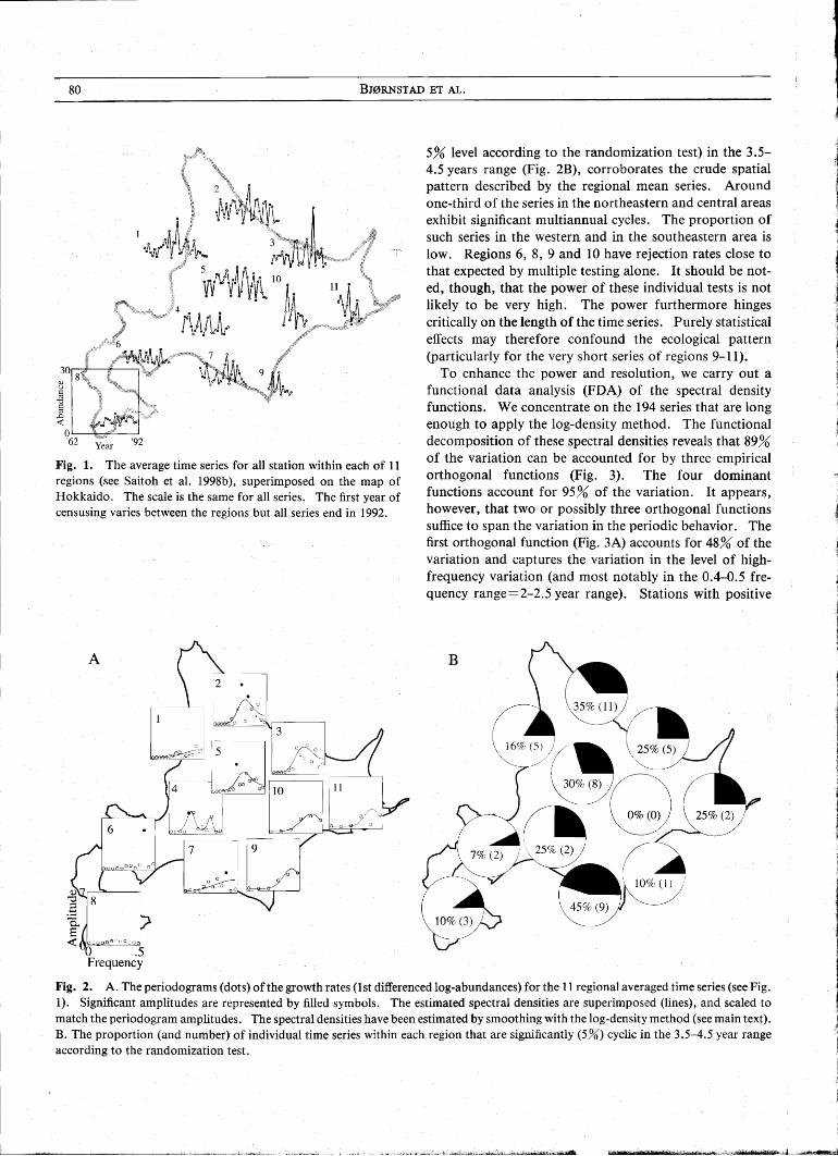
In the following we analyze the census counts stan­dardized to 150 trap-nights as the index of abundance (see Stenseth et al. 1996a; Saitoh et al. 1997). In order to help visualize the data we also group the 225 series into 11 broad regions within which the correlation between time series is relatively high (Saitoh et al. 1998b). The average time series for each of these 11 regions are shown in Fig. 1. The most violent flucluations are seen in the northeastern populations. The southwestern area harbors the most stable populations (see also Saitoh et al. 1998b).

Methods

In this study we focus on short-term periodic behavior likely to be induced by ecological interactions. Long-term behavior and trends are usually due to external forcing and anthropogenic influences requiring separate explanations (cf. Saitoh and Nakatsu 1997). To focus on the high frequency behavior we therefore study the population growth rates (the first differenced log-transformed data; see Bjernstad et al. 1996). A constant of unity was added to all counts prior to transformation.

The spectral density function, S(w), is the natural tool for considering frequency properties of a process (e.g. Priestley 1981). In terms of this function the process can be decomposed into sums of sine and cosine functions of varying frequencies w. The height (amplitude) of the spectral density function within a small frequency interval [Wi, Wi+ dWi] represents the proportion of the variability of the process attributable to periodic behavior with frequen­cies within this interval. Biogeographic variation in cyclicity implies that the spectral density of time series of abundance changes consistently across a region.

The simplest way to get an estimate of the spectral den­sity function of a time series of length T is by calculating the periodogram, I(w) , which is proportional to the squared correlation between the centered time series, {XI}, and the sinel cosine waves of a given frequency:

J( m) cc liT (~ x, sin( mt) r + 11 T (~ x, cos( mt) r For a discrete spectrum time series of the form

T12

X;= LAj cos(fj t)+Bj sin(fj t), j=l

(1)

(2)

where, jj are the discrete Fourier frequencies given by {fj= 2njlT, j= 1, ... , T12) , and Aj and Bj are Fourier coefficients, the periodogram satisfies l(fj) ex: Aj+ BJ (the constant of proportionality depends on the exact definition used; e.g. Chatfield 1989).

Note that since the periodogram, I(w), gives estimates of the spectral density function, S(w), at the discrete frequen­cies {fj}, the exact frequencies at which the spectral density is estimated depend on the length of the time series.

A noncyclic population will have a flat periodogram for the abundances. The individual amplitudes will be x2-

distributed under this null hypothesis. When studying the first-differenced log-abundances time series, the pattern in the amplitude is more complicated under the null (with a deficiency of low frequencies variability). There is no analytic test against this pattern. To test for significant cyclicity we therefore use a randomization test where we

REGIONAL TRANSITIONS IN VOLE DYNAMICS 79

permute the abundances prior to calculating the first differences and the subsequent periodograms (see Manly 1997: chapter 11). Note that in a collection of noncyclic populations, the null hypothesis should be rejected in 5% of the series due to multiple testing (at a nominal 5%­level).

The dependence on series length of the frequencies at which the periodogram is estimated makes it difficult to combine information from time series of different dura­tions. Another problem with the periodogram is that it does not provide a consistent estimate of the spectrum (that is, it does not converge to the true spectral density as the length of the time series increases; e.g. Wahba 1980). Therefore, it is better to work with direct estimates of the spectral density function, S(w).

To obtain a consistent estimate, S(w) , of the spectral density function, we make use of the following result (found in, e.g. Priestley 1981; see also Kooperberg et al. 1995). For a Gaussian process with true spectral density S(w), the amplitudes I(fj) of the periodogram are, asym­ptotically, independently distributed as S(fj) W, where W is exponentially distributed (except when j=O or j= T12, in which case W is chi-squared distributed with one degree of freedom). Thus, on a log-scale, the variation about the true spectral density is additive with constant variance and follows the distribution of log W (known as a Gumbel distribution). A consistent estimate of the spectral density function can thus be obtained by appropriate smoothing of the log periodogram. Natural splines provide the usual choice of basis functions for this smoothing (Wahba 1980; Kooperberg et al. 1995). In practice, we perform the smoothing by using quasilikelihood assuming the variance to be proportional to the squared-mean (as for the ex­ponential distribution) and with a log-link (Kooperberg et al. 1995; see also Hastie and Tibshirani 1990). For the 194 time series that are longer than 20 years, we optimize the estimated spectral density function (optimizing the num­ber and locations of spline knots according to the BIC criterion using the algorithm of Kooperberg et al. 1995). The 31 time series of length 12 are too short for this optimization, so we use a spline with fixed knots and 5 degrees-of-freedom (Kooperberg et al. 1995). All calcula­tions were done in S-plus version 3.3 (Statistical Sciences 1995); the log-density estimation was done using the LSPEC library (Kooperberg et al. 1995).

Once all the spectral density functions Siw) U= 1, ... , 225) have been calculated, we have a data-set composed of smooth functions from 225 different sites. Each "data­point" for further analysis is thus a curve or function. It is, therefore, natural to use functional data analysis (FDA) to describe the main types of functions (Ramsay and Sil­verman 1997). We want to decompose the 225 functions into a small number of empirical orthogonal functions (Castro et al. 1986; Ramsay and Silverman 1997). The

underlying idea is to find a small set of orthogonal func­tions, {Ui' i = 1, ... , p}, in terms of which all of the n curves can be described well through linear combinations:

p

SAw):::::: L ~jkUk(W). k=!

That is, we seek a set of principal functions which linear combinations (approximately) add up to the estimated spectral density functions. The method is analogous to a principal component analysis, but applied to functional data. The first principal orthogonal function accounts for the main axis of variation among the curves, and the sec­ond orthogonal function accounts for the subdominant axis of variation (under the constraint of orthogonality; Ramsay and Silverman 1997: chapter 6). Due to the way the calculations are done, it is usually possible to consider only a few of the orthogonal functions, which together explain most of the original variation. In the following we do the functional peA by discretizing the curves (sam­pled uniformly at 101 frequencies between 0 and 0,5; Cas­tro et al. 1986; Ramsay and Silverman 1997: chapter 6.4).

To visualize the decomposition we may examine the most important empirical orthogonal functions, u, directly. It is also illuminating to see how the overall mean function is affected by adding or subtracting a suitable multiple of each of the most important functions (Ramsay and Silverman 1997). The scores, ~jk> denote the coef­ficients for each site, j, for each orthogonal function, Uk>

that make up the linear combinations to span the spec­tral density. These numbers provide a classification of all sites along the principal axes of variation. Plotted on a map, these will highlight the main geographic variation in periodicity (Goodall 1954; Bj0rnstad et al. 1996).

Results

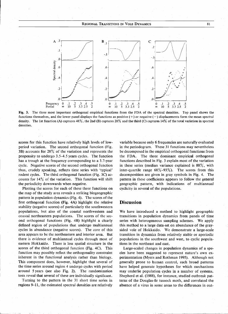
Figure 2 shows the periodograms (of the growth rates) of the 11 regional time series of vole abundance. The peaks in the northeastern and interior time series reflect multi­annual 3-4 year cycles in abundance (Fig. 2A; see Bj0rnstad et al. 1996), The randomization test reveals significant cyclicity with a 3.5-4.5 year period in regions 2 (P=O,03), 3 (P=0.08) and 5 (P=0.02). The 5.5-year cycle in region 4 is also highly significant (P< 0,01). This time series is unusual in exhibiting a bimodal spectrum. The dynamics in the western area is aperiodic (region 1) or cyclic with a 2.5-year period (regions 6 and 7; both P< 0.01). The extreme southwest (region 8) exhibits rela­tively stable dynamics. The estimated spectral density functions for the 11 regional time series are superimposed on the periodograms in Fig. 2A,

The proportion of individual time series and periodo­grams that harbors significant periodicity (at a nominal

80 BJ0RNSTAD ET AL.

Fig. 1. The average time series for all station within each of 11 regions (see Saitoh et al. 1998b), superimposed on the map of Hokkaido. The scale is the same for all series. The first year of censusing varies between the regions but all series end in 1992.

A

.g

.~

J cooooaGcceo?

o .5 Frequency

5% level according to the randomization test) in the 3.5-4.5 years range (Fig. 2B), corroborates the crude spatial pattern described by the regional mean series. Around one-third of the series in the northeastern and central areas exhibit significant multiannual cycles. The proportion of such series in the western and in the southeastern area is low. Regions 6, 8, 9 and 10 have rejection rates close to that expected by multiple testing alone. It should be not­ed, though, that the power of these individual tests is not likely to be very high. The power furthermore hinges critically on the length of the time series. Purely statistical effects may therefore confound the ecological pattern (particularly for the very short series of regions 9-11).

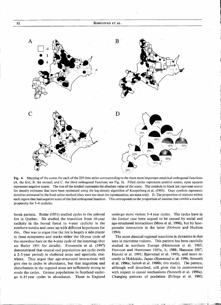
To enhance the power and resolution, we carry out a functional data analysis (FDA) of the spectral density functions. We concentrate on the 194 series that are long enough to apply the log-density method. The functional decomposition of these spectral densities reveals that 89% of the variation can be accounted for by three empirical orthogonal functions (Fig. 3). The four dominant functions account for 95% of the variation. It appears, however, that two or possibly three orthogonal functions suffice to span the variation in the periodic behavior. The first orthogonal function (Fig. 3A) accounts for 48% of the variation and captures the variation in the level of high­frequency variation (and most notably in the 0.4-0.5 fre­quency range=2-2.5 year range). Stations with positive

Fig. 2. A. The periodograms (dots) ofthe growth rates (1st differenced log-abundances) for the 11 regional averaged time series (see Fig. 1). Significant amplitudes are represented by filled symbols. The estimated spectral densities are superimposed (lines), and scaled to match the periodogram amplitUdes. The spectral densities have been estimated by smoothing with the log-density method (see main text). B. The proportion (and number) of individual time series within each region that are significantly (5%) cyclic in the 3.5-4.5 year range according to the randomization test.

REGIONAL TRANSITIONS IN VOLE DYNAMICS 81

A .2

.1

.0 .£ ~

.6 (!) "0 (;3 b u (!)

.4 0.. Vl

#1++++ .6 + ++

++ + ++ ++

++ .4 -+

++ + +-

.6 + +

++ + + + +

.4 + + F

.2

+ -+ +

.2 + ++-i"!"+

+ +,

.0 L,.-----,--r----r----,-....,..J

Frequency 0 .1 .2 .3 .4 .5 Period 00 10 5 3.3 2.5 2

o .1 .2 .3 .4 .5 00 10 5 3.3 2.5 2

o .1 .2 .3 .4 .5 00 10 5 3.3 2.5 2

Fig. 3. The three most important orthogonal empirical functions from the FDA of the spectral densities. Top panel shows the functions themselves, and the lower panel displays the functions as positive ( + ) or negative ( - ) displacements form the mean spectral density. The 1st function (A) captures 48%, the 2nd (B) captures 28% and the third (C) captures 14% of the total variation in spectral densities.

scores for this function have relatively high levels of low­period variation. The second orthogonal function (Fig. 3B) accounts for 28% of the variation and represents the propensity to undergo 3.5-4.5 years cycles. The function has a trough at the frequency corresponding to a 3.7 -year cycle. Negative scores of the second orthogonal function thus, crudely speaking, reflects time series with 'typical' rodent cycles. The third orthogonal function (Fig. 3C) ac­counts for 14% of the variation. This function will shift the periodicity downwards when negative.

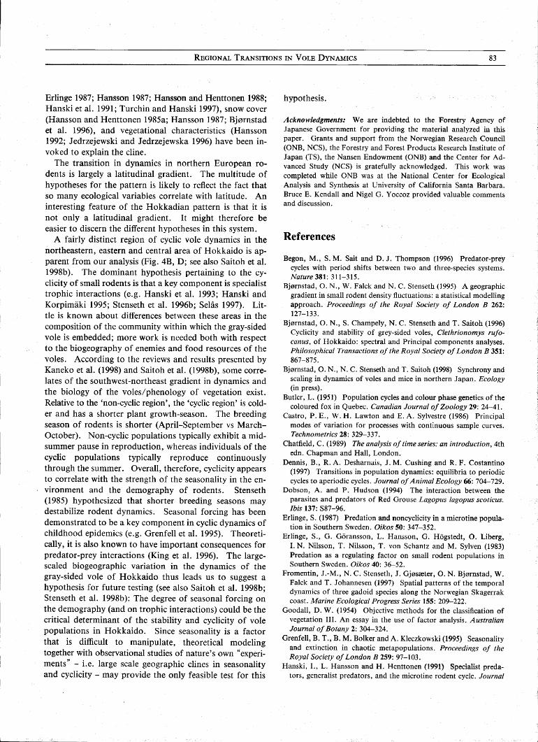
Plotting the scores for each of these three functions on the map of the study area reveals a striking biogeographic pattern in population dynamics (Fig. 4). The scores of the first orthogonal function (Fig. 4A) highlight the relative stability (negative scores) of particularly the southwestern populations, but also of the coastal northwestern and coastal northeastern populations. The scores of the sec­ond orthogonal functions (Fig. 4B) highlight a clearly defined region of populations that undergo multiannual cycles in abundance (negative scores). The core of this area appears to be the northeastern and interior area. But there is evidence of multiannual cycles through most of eastern Hokkaido. There is less spatial structure in the scores of the third orthogonal function (Fig. 4C). This function may possibly reflect the orthogonality constraint inherent in the functional analysis rather than biology. This component does, however, highlight that several of the time series around region 4 undergo cycles with period around 5 years (see also Fig. 2). The randomization tests reveal that several of these are individually significant.

Turning to the pattern in the 31 short time series in regions 9-11, the estimated spectral densities are relatively

variable because only 6 frequencies are naturally evaluated in the periodogram. These 31 functions may nevertheless be decomposed in the empirical orthogonal functions from the FDA. The three dominant empirical orthogonal functions described in Fig. 3 explain most of the variation in these series (median variance explained is 88%, with inter-quartile range 68%-93%). The scores from this decomposition are given in gray symbols in Fig. 4. The pattern in these coefficients appears to follow the general geographic pattern, with indications of multi annual cyclicity in several of the populations.

Discussion

We have introduced a method to highlight geographic transitions in population dynamics from panels of time series with heterogeneous sampling schemes. We apply this method to a large data-set on abundance of the gray­sided vole of Hokkaido. We demonstrate a large-scale transition in dynamics from relatively stable or aperiodic populations in the southwest and west, to cyclic popula­tions in the northeast and east.

Large-scaled changes in population dynamics of a spe­cies have been suggested to represent nature's own ex­perimentation (Myers and Rothman 1995). Although not generally prone to human control, such broad patterns have helped generate hypotheses for which mechanisms may underlie population cycles in a number of systems. Shepherd et al. (1988), for instance, studied outbreak pat­terns of the Douglas-fir tussock moth, and correlated the absence of a virus in some areas to the differences in out-

82 BJ0RNSTAD ET AL.

A

0-4

• 1 .4

D

Fig. 4. Mapping of the scores for each of the 225 time series corresponding to the three most important empirical orthogonal functions (A. the first; B. the second; and C. the third orthogonal function; see Fig. 3). Filled circles represents positive scores, open squares represents negative scores. The size of the symbol represents the absolute value of the score. The symbols in black ink represent scores for density estimates that have been optimized using the log-density algorithm of Kooperberg et al. (1995). Gray symbols represents densities estimated by the fixed spline method (they were too short for optimization; see main text). D. The proportion of stations within each region that had negative score of the 2nd orthogonal function. This corresponds to the proportion of stations that exhibit a marked propensity for 3-4 cyclicity.

break pattern. Butler (1951) studied cycles in the colored fox in Quebec. He studied the transition from 10-year cyclicity in the boreal forest to 4-year cyclicity in the northern tundra and came up with different hypotheses for this. One was to argue that the fox is largely a side-player in these ecosystems and tracks either the 10-year cycle of the snowshoe hare or the 4-year cycle of the lemmings (but see Butler 1951 for details). Fromentin et al. (1997) demonstrated that coastal cod populations are cyclic (with a 2-3-year period) in sheltered areas and aperiodic else­where. They argue that age-structured interactions will give rise to cycles in abundance, but that migration and disturbances in the exposed areas are sufficiently strong to erode the cycles. Grouse populations in Scotland under­go 6-15 year cycles in abundance. Those in England

undergo more violent 3-4 year cycles. The cycles have in the former case been argued to be caused by social and age-structured interactions (Moss et al. 1996), but by host­parasite interaction in the latter (Dobson and Hudson 1994).

The most classical regional transition in dynamics is that seen in microtine rodents. This pattern has been carefully studied in northern Europe (Henttonen et al. 1985; Hansson and Henttonen 1985a, b, 1988; Hansson 1987; Hanski et al. 1991; Bj0rnstad et al. 1995), and more re­cently in Hokkaido, Japan (Bj0rnstad et al. 1996; Stenseth et al. 1996a; Saitoh et al. 1998b; this study). The pattern, although well described, still gives rise to controversies with respect to causal mechanisms (Stenseth et al. 1998a). Changing patterns of predation (Erlinge et al. 1983;

REGIONAL TRANSITIONS IN VOLE DYNAMICS 83

Erlinge 1987; Hansson 1987; Hansson and Henttonen 1988; Hanski et al. 1991; Turchin and Hanski 1997), snow cover (Hansson and Henttonen 1985a; Hansson 1987; Bj0rnstad et al. 1996), and vegetational characteristics (Hansson 1992; ledrzejewski and ledrzejewska 1996) have been in­voked to explain the cline.

The transition in dynamics in northern European ro­dents is largely a latitudinal gradient. The multitude of hypotheses for the pattern is likely to reflect the fact that so many ecological variables correlate with latitude. An interesting feature of the Hokkadian pattern is that it is not only a latitudinal gradient. It might therefore be easier to discern the different hypotheses in this system.

A fairly distinct region of cyclic vole dynamics in the northeastern, eastern and central area of Hokkaido is ap­parent from our analysis (Fig. 4B, D; see also Saitoh et al. 1998b). The dominant hypothesis pertaining to the cy­clicity of small rodents is that a key component is specialist trophic interactions (e.g. Hanski et al. 1993; Hanski and Korpimaki 1995; Stenseth et al. 1996b; Selas 1997). Lit­tle is known about differences between these areas in the composition of the community within which the gray-sided vole is embedded; more work is needed both with respect to the biogeography of enemies and food resources of the voles. According to the reviews and results presented by Kaneko et al. (1998) and Saitoh et al. (1998b), some corre­lates of the southwest-northeast gradient in dynamics and the biology of the voles/phenology of vegetation exist. Relative to the 'non-cyclic region', the 'cyclic region' is cold­er and has a shorter plant growth-season. The breeding season of rodents is shorter (April-September vs March­October). Non-cyclic populations typically exhibit a mid­summer pause in reproduction, whereas individuals of the cyclic populations typically reproduce continuously through the summer. Overall, therefore, cyclicity appears to correlate with the strength of the seasonality in the en­vironment and the demography of rodents. Stenseth (1985) hypothesized that shorter breeding seasons may destabilize rodent dynamics. Seasonal forcing has been demonstrated to be a key component in cyclic dynamics of childhood epidemics (e.g. Grenfell et al. 1995). Theoreti­cally, it is also known to have important consequences for predator-prey interactions (King et al. 1996). The large­scaled biogeographic variation in the dynamics of the gray-sided vole of Hokkaido thus leads us to suggest a hypothesis for future testing (see also Saitoh et al. 1998b; Stenseth et al. 1998b): The degree of seasonal forcing on the demography (and on trophic interactions) could be the critical determinant of the stability and cyclicity of vole populations in Hokkaido. Since seasonality is a factor that is difficult to manipulate, theoretical modeling together with observational studies of nature's own "experi­ments" - i.e. large scale geographic clines in seasonality and cyclicity - may provide the only feasible test for this

hypothesis.

Acknowledgments: We are indebted to the Forestry Agency of Japanese Government for providing the material analyzed in this paper. Grants and support from the Norwegian Research Council (ONB, NCS), the Forestry and Forest Products Research Institute of Japan (TS), the Nansen Endowment (ONB) and the Center for Ad­vanced Study (NCS) is gratefully acknowledged. This work was completed while ONB was at the National Center for Ecological Analysis and Synthesis at University of California Santa Barbara. Bruce E. Kendall and Nigel G. Y occoz provided valuable comments and discussion.

References

Begon, M., S. M. Sait and D. J. Thompson (1996) Predator-prey cycles with period shifts between two and three-species systems. Nature 381: 311-315.

Bj0rnstad, O. N., W. Falck and N. C. Stenseth (1995) A geographic gradient in small rodent density fluctuations: a statistical modelling approach. Proceedings of the Royal Society of London B 262: 127-133.

Bj0rnstad, O. N., S. Champely, N. C. Stenseth and T. Saitoh (1996) Cyclicity and stability of grey-sided voles, Clethrionomys rufo­canus, of Hokkaido: spectral and Principal components analyses. Philosophical Transactions of the Royal Society of London B 351: 867-875.

Bj0rnstad, O. N., N. C. Stenseth and T. Saitoh (1998) Synchrony and scaling in dynamics of voles and mice in northern Japan. Ecology (in press).

Butler, L. (1951) Population cycles and colour phase genetics of the coloured fox in Quebec. Canadian Journal of Zoology 29: 24-41.

Castro, P. E., W. H. Lawton and E. A. Sylvestre (1986) Principal modes of variation for processes with continuous sample curves. Technometrics 28: 329-337.

Chatfield, C. (1989) The analysis of time series: an introduction, 4th edn. Chapman and Hall, London.

Dennis, B., R. A. Desharnais, J. M. Cushing and R. F. Costantino (1997) Transitions in population dynamics: equilibria to periodic cycles to aperiodic cycles. Journal of Animal Ecology 66: 704-729.

Dobson, A. and P. Hudson (1994) The interaction between the parasites and predators of Red Grouse Lagopus /agopus scoticus. Ibis 137: S87-96.

Erlinge, S. (1987) Predation and noncyclicity in a microtine popula­tion in Southern Sweden. Oikos 50: 347-352.

Erlinge, S., G. Goransson, L. Hansson, G. Hogstedt, O. Liberg, I. N. Nilsson, T. Nilsson, T. von Schantz and M. Sylven (1983) Predation as a regulating factor on small rodent populations in Southern Sweden. Oikos 40: 36-52.

Fromentin, J.-M., N. C. Stenseth, J. Gj0sreter, O. N. Bj0rnstad, W. Falck and T. Johannesen (1997) Spatial patterns of the temporal dynamics of three gadoid species along the Norwegian Skagerrak coast. Marine Ecological Progress Series 155: 209-222.

Goodall, D. W. (1954) Objective methods for the classification of vegetation III. An essay in the use of factor analysis. Australian Journal of Botany 2: 304-324.

Grenfell, B. T., B. M. Bolker and A. Kleczkowski (1995) Seasonality and extinction in chaotic metapopulations. Proceedings of the Royal Society of London B 259: 97-103.

Hanski, I., L. Hansson and H. Henttonen (1991) Specialist preda­tors, generalist predators, and the microtine rodent cycle. Journal

84 BJ0RNSTAD ET AL.

oj Animal Ecology 60: 353-367. Hanski, I. and E. Korpimaki (1995) Microtine rodent dynamics in

Northern Europe: Parametrized models for the predator-prey in­teraction. Ecology 76: 840-850.

Hanski, I., P. Turchin, E. Korpimaki and H. Henttonen (1993) Population oscillations of boreal rodents: Regulation by mustelid predators leads to chaos. Nature 364: 232-235.

Hansson, L. (1987) An interpretation of rodent dynamics as due to trophic interactions. Oikos 50: 308-318.

Hansson, L. (1992) Small mammal communities on clearcuts in a latitudinal gradient. Acta Oecologia 13: 687-699.

Hansson, L. and H. Henttonen (1985a) Gradients in density varia­tions of small rodents: the importance of latitude snow cover. Oecologia 67: 394-402.

Hansson, L. and H. Henttonen (1985b) Regional differences in cy­clicity and reproduction in Clethrionomys species: Are they relat­ed? Annales Zoologica Fennici 22: 277-288.

Hansson, L. and H. Henttonen (1988) Rodent dynamics as com­munity processes. Trends in Ecology and Evolution 3: 195-200.

Hastie, T. and R. Tibshirani (1990) Generalized additive models. Chapman and Hall, London.

Hastings, A., C. L. Hom, S. Ellner, P. Turchin and H. C. J. Godfray (1993) Chaos in ecology: Is mother nature a strange attractor? Annual Review oj Ecology and Systematics 24: 1-33.

Henttonen, H., D. McGuire and L. Hansson (1985) Comparisons of amplitude and frequencies (spectral analyses) of density variations in long-term data sets of Clethrionomys species. Annales Zoologica Fennici 22: 221-27.

Jedrzejewski, W. and B. Jedrzejewska (1996) Rodent cycles in rela­tion to biomass and productivity of ground vegetation and preda­tion in the Palearctic. Acta Theriologica 41: 1-34.

Kaneko, Y., K. Nakata, T. Saitoh, N. C. Stenseth and O. N. Bj0rnstad (1998) The biology of the vole Clethrionomys ruJo­canus: a review. Researches on Population Ecology 40: 21-37.

King, A. A., W. M. Schaffer, C. Gordon, J. Treat and M. Kot (1996) Weakly dissipative predator-prey systems. Bulletin oj Mathemati­cal Biology 58: 835-859.

Kooperberg, C., C. J. Stone and Y. K. Truong (1995) Logspline es­timation of a possibly mixed spectral distribution. Journal oj Time Series Analysis 16: 359-388.

Manly, B. F. J. (1997) Randomization, bootstrap and Monte Carlo methods in biology, 2nd edn. Chapman and Hall, London.

May, R. M. (1976) Simple mathematical models with very compli­cated dynamics. Nature 261: 459-467.

Moss, R., A. Watson and R. Parr (1996) Experimental prevention of population cycle in red grouse. Ecology 77: 1512-1530.

Murdoch, W. W. and C. J. Briggs (1996) Theory of biological con­trol: recent developments. Ecology 77: 2001-2013.

Myers, J. H. and L. D. Rothman (1995) Field experiments to study regulation of fluctuating populations. pp. 229-251. In N. Cappuc­cino and P. Price (eds.) Population dynamics. Academic Press, New York.

Priestley, M. B. (1981) Spectral analysis and time series. Academic Press, London.

Ramsay, J. O. and B. W. Silverman (1997) Functional data analysis. Springer-Verlag, New York.

Saitoh, T. and A. Nakatsu (1997) Impact of forest plantation on the community of small mammals in Hokkaido, Japan. Mammal Study 22: 27-38.

Saitoh, T., N. C. Stenseth and O. N. Bj0rnstad (1997) Density dependence in fluctuating grey-sided vole populations. Journal oJ Animal Ecology 66: 14-24.

Saitoh, T., O. N. Bj0rnstad and N. C. Stenseth (1998a) Density­dependence in voles and mice: a comparative analysis. Ecology (in press).

Saitoh, T., N. C. Stenseth and O. N. Bj0rnstad (1998b) The popula­tion dynamics of the vole, Clethrionomys ruJocanus, in Hokkaido Japan. Researches on Population Ecology 40: 61-76.

Seliis, V. (1997) Cyclic population fluctuations of herbivores as an effect of cyclic seed cropping of plants: the mast depression hypothesis. Oikos 80: 257-268.

Shepherd, R., D. D. Bennet, J. W. Dale, S. Tunnock, R. E. Dolph and R. W. Thier (1988) Evidence of synchronized cycles in out­break patterns of Douglas-fir tussock moth, Orgyia pseudotsugata (McDunnough) (Lepidoptera: Lymantriidae). Memoirs oj the Entomological Society oJ Canada, Ottawa 146: 107-121.

Statistical Sciences (1995) S-plus guide to statistical and mathemati­cal analysis, version 3.3. StatSci, MathSoft, Inc., Seattle.

Stenseth, N. C. (1985) Models of bank vole and wood mice. Sym­posium oj the Zoological Society oj London 55: 339-376.

Stenseth, N. C., O. N. Bj0rnstad and T. Saitoh (1996a) A gradient from stable to cyclic populations of Clethrionomys ruJocanus in Hokkaido, Japan. Proceedings oj the Royal Society oj London B 263: 1117-1126.

Stenseth, N. C., O. N. Bj0rnstad and W. Falck (1996b) Is spacing behaviour coupled with predation causing the micro tine density cycle? A synthesis of current process-oriented and pattern-oriented studies. Proceedings oj the Royal Society oj London B 263: 1423-1435.

Stenseth, N. C., O. N. Bj0rnstad and T. Saitoh (1998a) Seasonal forcing on the dynamics of Clethrionomys ruJocanus: modeling geographic gradients in population dynamics. Researches on Population Ecology 40: 85-95.

Stenseth, N. C., T. Saitoh and N. G. Yoccoz (1998b) Frontiers of population ecology in microtine rodents: a pluralistic approach to the study of population ecology. Researches on Population Ecolo­gy 40: 5-20.

Turchin, P. and I. Hanski (1997) An empirically based model for latitudinal gradient in vole population dynamics. American Naturalist 149: 842-874.

Wahba, G. (1980) Automatic smoothing of the log periodogram. Journal oj the American Statistical Association 75: 122-132.

Received 28 April 1998; Accepted 27 May 1998

I I