Mapping Viscoelastic and Plastic Properties of Polymers ...

VEP Mapping 4/29/2016 Page 1 of 28

Mapping Viscoelastic and Plastic Properties of

Polymers and Polymer-Nanotube Composites using Instrumented Indentation

Andrew J. Gayle, Robert F. Cooka)

Materials Measurement Science Division, National Institute of Standards and Technology,

Gaithersburg, MD 20899, USA

Abstract: An instrumented indentation method is developed for generating maps of time-

dependent viscoelastic and time-independent plastic properties of polymeric materials. The

method is based on a pyramidal indentation model consisting of two quadratic viscoelastic

Kelvin-like elements and a quadratic plastic element in series. Closed-form solutions for

indentation displacement under constant load and constant loading-rate are developed and used

to determine and validate material properties. Model parameters are determined by point

measurements on common monolithic polymers. Mapping is demonstrated on an epoxy-ceramic

interface and on two composite materials consisting of epoxy matrices containing multi-wall

carbon nanotubes. A fast viscoelastic deformation process in the epoxy was unaffected by the

inclusion of the nanotubes, whereas a slow viscoelastic process was significantly impeded, as

was the plastic deformation. Mapping revealed considerable spatial heterogeneity in the slow

viscoelastic and plastic responses in the composites, particularly in the material with a greater

fraction of nanotubes.

Online Abstract Figure: Fig. 10(b)

Key Words: nano-indentation, polymer, composite

a)Address all correspondence to this author.

e-mail: [email protected]

Revision submitted to

Journal of Materials Research

April, 2016


I. INTRODUCTION

Indentation of polymeric or biological materials or their composites frequently leads to

three concurrent modes of contact deformation, characterized by three different variations of the

indenter displacement into the material, h, with indentation load, P, and time, t:1-12

(V) Viscous deformation, in which the indenter displacement is time-dependent,

typically with the rate of displacement varying with load.

(E) Elastic deformation, in which the indenter displacement is time-independent and

recovers completely on load removal.

(P) Plastic deformation, in which the indenter displacement is time-independent and

does not recover at all on load removal.

Indentation with a spherical probe or flat punch often suppresses plastic deformation such that

the deformation is completely viscoelastic,6,11,13-20 or is assumed so for fluid-like

materials.14,15,21,22 Under these conditions, viscoelastic correspondence principles23-27 can be used

to predict the h(t) response from an imposed P(t) spectrum (or vice versa) if the purely elastic

P(h) indentation behavior is known and a time-dependent creep (or relaxation) function is

selected for the material. The predictions are frequently framed in terms of superposition

integrals. Indentation with the more-commonly used pyramidal probes, such as the three-sided

Berkovich diamond, usually generates all three of the viscous-elastic-plastic (VEP) indentation

deformations. Under these conditions, correspondence principles, which rely on material

linearity in elastic and viscous constitutive behavior (Hookean and Newtonian, respectively),

cannot be used as the plasticity renders the non-viscous component of the deformation non-

linear. Hence, although correspondence methods can incorporate the geometrical non-linearity of

spherical and pyramidal indentation, in which the indentation contact area increases with

indentation depth,25 plastic deformation precludes their use.

The original VEP indentation model incorporated the geometrical non-linearity of

pyramidal indentation explicitly into each component of the deformation,1 treating each

displacement component separately. The plastic displacement, hP(t), was given by

[ ] 2/11maxP /)()( HtPth α= (1)

where Pmax(t) is the maximum load experienced over the time interval t, α1 is a dimensionless

indenter geometry constant, and H is the resistance to plastic deformation. For an elastic-

perfectly plastic material H is the hardness. The elastic displacement, hE(t), was given by


[ ] 2/12E /)()( MtPth α= (2)

where α2 is another dimensionless indenter geometry constant, and M is the resistance to elastic

deformation. For an elastic material M is the indentation modulus. The viscous displacement,

hV(t), was expressed as a rate,

[ ] 2/122V /)(d/)(d τα MtPtth = (3)

where τ is the time constant for viscous flow. The term α2Mτ2 is an effective quadratic viscosity.

(Eqs. (2) and (3) use the more recent notation.4) The total indentation displacement was taken as

the sum

h = hE + hP + hV (4)

such that the overall indentation model could be viewed as a generalized quadratic “Maxwell”-

like model of elements in series. For simple loading schemes, such as triangular, linear load-

unload, spectra, the integral implicit in Eq. (3) is simply performed and the total displacement

given by Eq. (4) can be expressed in closed form. The simplicity of this formulation allows the

resistance to the three different modes of deformation to be scaled separately via H, M, and τ,

such that the complete variety of material indentation load-displacement responses can be

described and analyzed.4,6

The quadratic Maxwell VEP model above was reasonably successful in a quantitative

sense: the material properties H, M, and τ inferred from fits of the model to triangular load

spectra, specifically fits to the unloading response in which all three displacement components

are distinct, were in agreement with other measurements;1,2,5 the ability of the model to predict

loading behavior from unloading behavior was excellent;1,2,4,5,8 and, the material properties

inferred using a triangular load spectrum at a reference time- or load-scale could be used to

predict the triangular responses for indentation time scales factors of three shorter or longer than

the reference and indention load scales factors of ten different from the reference.1,2,4,8 The

limitations of the quadratic Maxwell VEP model are apparent in comparisons of observed and

predicted behavior during constant-load creep, a test method that focuses on the time-dependent

constitutive behavior. The free viscous element, meaning that it has no element constraining it in

parallel, of the quadratic Maxwell VEP model leads to unbounded displacement increasing

linearly with time for an imposed constant load and an instantaneous displacement recovery on

load removal.1 Neither of these phenomena are observed during indentation of the vast majority


of polymeric and biological materials: Displacement rates during constant-load creep decrease

with time such that the displacement approaches a bounded value at long times1,3,7,9,11,12,20 and

recovery on load removal is not instantaneous but occurs over time scales comparable to those

required to reach the bounded creep displacement.9,12 Furthermore, the time-dependent

indentation creep and recovery behavior of most polymeric and biological materials is not well

described by a single time constant, but by two or more.3,9,12,16,18-20

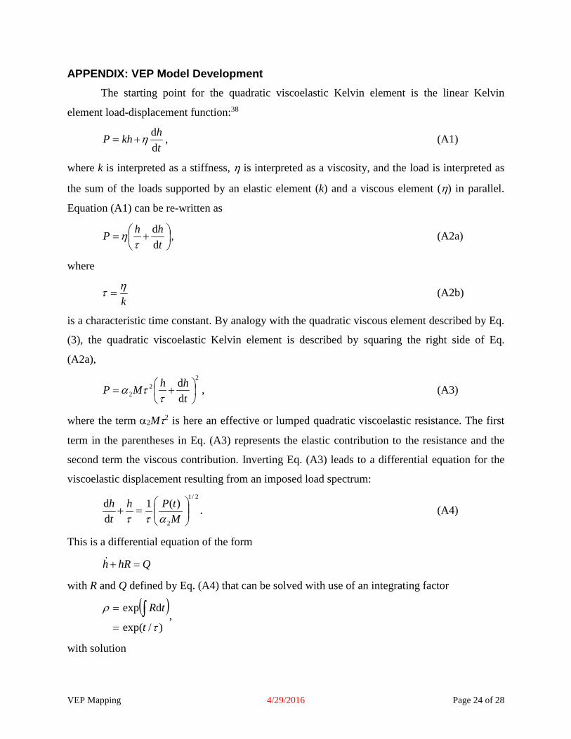
Here, a new VEP pyramidal indentation model and analysis is developed that is similar in

spirit to the original model (elements in series, closed form displacement expressions, simple

identification of material behavior dependencies) but which overcomes the deficiencies noted

above. As foreshadowed earlier,4 the model is based on a quadratic “Kelvin”-like element, in

which the viscous element is bounded by an elastic element in parallel, such that displacement

during constant-load creep is bounded and displacement recovery on load removal is not

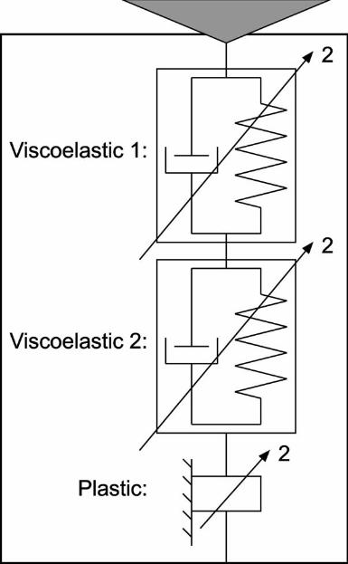
instantaneous. Two such viscoelastic elements are combined in series to provide for deformation

over two time scales, along with a third, plastic, element in series as before. A schematic diagram

of the full quadratic Kelvin VEP model is shown in Fig. 1. The model is nearly identical to that

recently implemented by Mazeran et al.9 and Isaza et al.,12 with the omission of the fourth

quadratic Maxwell element used by Mazeran, Isaza et al. to describe a viscoplastic response. In

the original VEP model, the behavior of the single-time-constant viscous element could be

deconvoluted unambiguously from the indentation unloading response of a simple load triangle.

The extra degree of freedom associated with the two time constants of the two viscoelastic

elements in Fig. 1 precludes such simple deconvolution and a more extensive testing protocol is

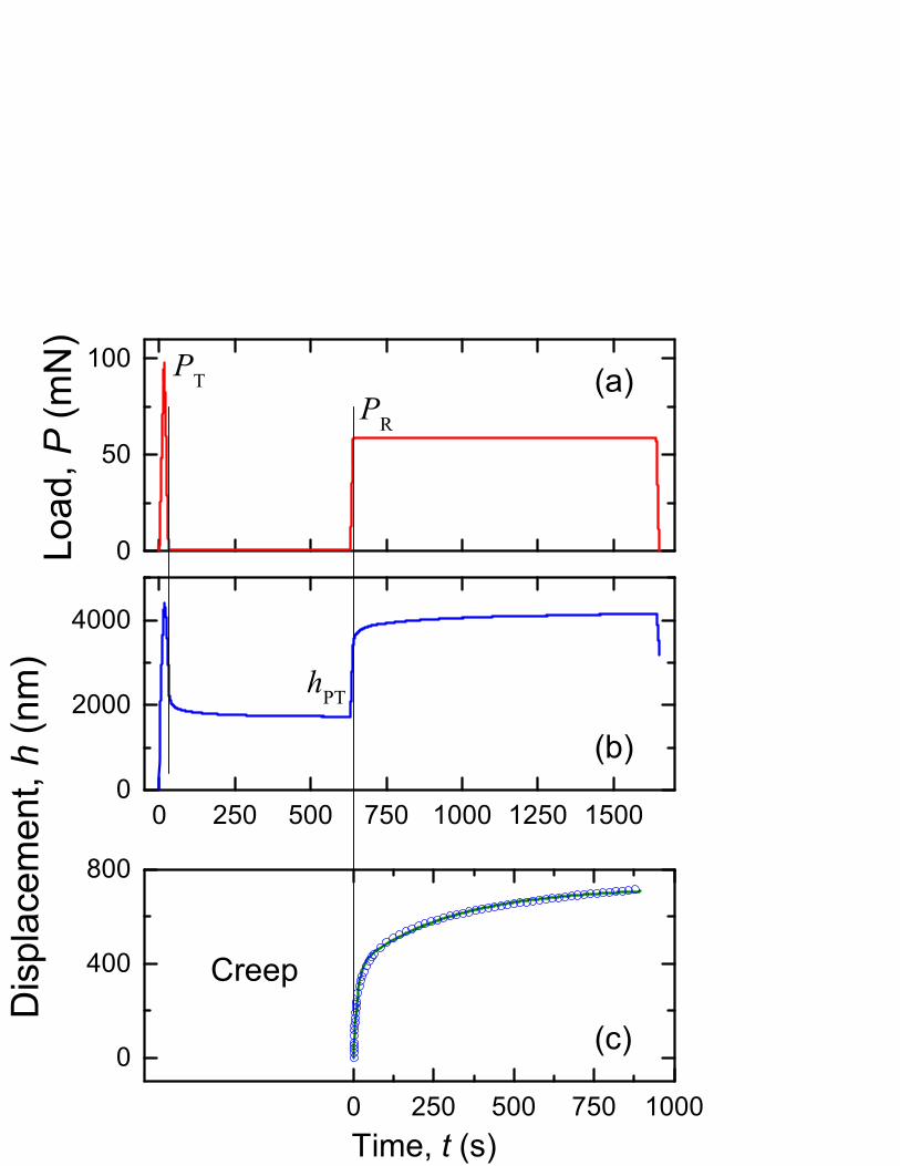
required. Here, a three-segment load spectrum is used as shown in Fig. 2(a): (1) a triangle wave,

followed by (2) a near-zero load hold, followed by (3) a trapezoidal load wave. The protocol is

identical to that used by Zhang et al.3 for exactly the same reasons: the final trapezoidal segment

isolates the viscoelastic response under constant-load conditions that are simple to analyze.

A major motivation for the development of the new model and analysis was to map the

mechanical properties of polymer-carbon nanotube (CNT) composites. Such composites have

great potential as lightweight mechanical or electrical materials that take advantage of the high

stiffness and strength or electrical conductivity of CNTs, respectively. As with all composites,

appropriate dispersion of the minority enhancing phase in the majority matrix phase is critical to

obtaining desired properties: For example, the stiff CNTs must be dispersed and bound to the


compliant polymer matrix so as to achieve stress transfer and stiffening of the composite; the

conducting CNTs must be dispersed so as to percolate throughout the insulating polymer matrix

so as to obtain a conducting structure. As a consequence, considerations of CNT dispersion in

polymer matrices have been the subject of much study since the early applications of CNTs.28-31

The goal here was to develop an instrumented indentation testing (IIT) method that could

provide a direct measure of the mechanical behavior of polymer-CNT composites in the form of

two-dimensional maps of viscoelastic and plastic properties. Such maps take advantage of the

local probing capabilities of IIT and have been used to explore the effects of microstructure on

spatial variations of mechanical properties in ceramic-metal composites,32 tooth enamel,33

bone,34 cement paste and rocks,35 and metals.36,37 In these cases, time-dependent deformation

was not considered and elastic and plastic properties were mapped. The next section develops the

new VEP indentation model and expressions for h(t) that allow material properties to be

determined from simple P(t) protocols. The following sections then demonstrate and validate the

applicability of the model in single-point tests on monolithic polymers and glass. The mapping

capability is then demonstrated in multi-point tests on a ceramic-polymer interface and two

polymer-CNT composites. Finally, possible extensions of the model and protocols are discussed.

II. MATERIALS AND METHODS A. Materials

Five common commercial polymeric materials were obtained in approximately 1 mm

thick solid sheet form. The materials were a high-density polyethylene (HDPE), two poly(methyl

methacrylate)s (PMMA1, and PMMA2), a polystyrene (PS), and a polycarbonate (PC). Samples

approximately 15 mm × 15 mm were cut from the sheets and fixed to aluminum pucks for IIT

measurements. The surfaces of the samples were highly reflective and tested in the as-received

state, except for the HDPE, which was diamond polished to a reflective state. A commercial

soda-lime silicate glass (SLG) microscope slide was also tested.

Two commercial epoxy materials were obtained in liquid form as separate resins and

curing agents. The first (Epoxy 1) consisted of Epon 828 resin (miller-stephenson, Danbury, CT)

and Ancamide 507 curing agent (Air Products, Allentown, PA). The resin and curing agent were

mixed in the proportion 3:1 by mass and samples approximately 5 mm thick cast into circular

plastic molds 35 mm in diameter, allowed to cure at room temperature for 48 h, and then


removed from the molds. The surfaces cast against the base of the molds were highly reflective

and tested in the as-cast state. The second (Epoxy2) consisted of a resin and curing agent used

for metallographic sample preparation, mixed as directed by the supplier (Buehler, Lake Bluff,

IL), cast into a circular plastic mold along with a piece of dense AlN ceramic, and allowed to

cure as directed. The composite sample was removed from the mold and diamond polished to a

reflective state such that a sharp epoxy-ceramic interface was normal to the sample surface.

Two epoxy-CNT composite materials were obtained from a commercial vendor. The

composites consisted of mass fractions of 1 % and 5 % of multi-wall CNT (MWCNT) mixed

into an epoxy matrix equivalent to Epoxy1 above. In order to enable direct comparison with the

mechanical properties of the matrix epoxy, no chemical additives to improve homogeneity of

MWCNT dispersion were included in the composites; it was thus expected that the MWCNT

dispersion would be somewhat inhomogeneous.29,30 The composite material samples were in the

form of 15 mm × 15 mm sheets approximately 0.5 mm thick and were fixed to aluminum pucks

with Epoxy1 for IIT measurements. The surfaces of the samples were reflective and tested in the

as-received state.

B. Experimental Methods Single-point IIT measurements of the monolithic materials were used to establish and

validate the experimental and analytical methods in two sequential stages. In the first stage,

indentation displacements were measured during a three-segment applied load spectrum as

described above. Material properties were determined from these measurements. In the second

stage, indentation displacements were predicted from these properties for a range of single-

segment linear load ramps and compared with experimental measurements; the property values

were also compared with accepted values for the materials. In this way, the validity of both the

form of the analysis and the magnitude of the included parameters could be assessed. A

Berkovich diamond probe was used for all experiments. The data collection rate for load,

displacement, and time for all experiments was at least 10 Hz.

The first-stage, three-segment applied load spectrum was as follows:

1. A triangular segment, consisting of a linear load ramp from zero to a peak load of PT and

then a linear ramp back to near zero over a total period of approximately 30 s; the end of

this segment is indicated by the left vertical line in Fig. 2. PT = 100 mN was used. The


displacement response for PMMA1 is shown in Fig. 2(b) and consisted of an increase from

zero to a peak displacement followed by a decrease to a non-zero displacement at the end

of the segment.

2. A period of near zero load, approximately 1 mN, typically extending for 600 s. The

displacement response for PMMA1 is shown in Fig. 2(b) and consisted of recovery to a

near invariant displacement, hPT, at the end of the segment.

3. A trapezoidal segment consisting of a linear ramp from near zero load to peak load of PR <

PT in a time of tR, a long creep load-hold period at PR, and a linear ramp to zero load. PR =

60 mN and tR ≈ 10 s were used and the creep hold period was typically 1000 s; the

beginning of the creep hold period is indicated by the right vertical line in Fig. 2. The

displacement response for PMMA1 is shown in Fig. 2(b) and consisted of a rapid increase

in displacement followed by a slower increase to near invariant displacement at the end of

the creep hold. An expanded view of the slower creep displacement response is shown in

shifted creep coordinates in Fig. 2(c) (setting the creep time to 0 after the tR ≈ 10 s rise to

the creep load); analysis of such data provided the majority of the material viscoelastic

information.

At least four three-segment spectra were measured and analyzed for each material. Prior to

measurement, preliminary trapezoidal experiments were used to ascertain the characteristic time

scales for deformation.

The second-stage validation experiments were a series of linear load ramps. The ramps

were part of a triangular load wave as illustrated in the initial segment of Fig. 1(a), with the

exceptions that the peak loads were variable values PU and the rise times were much longer

variable values tU. (The subscript “U” indicates that these validation conditions are in principle

unknown during the above first-stage measurements.) Only the loading parts of the triangle

waves were used in the validation experiments. Two different forms of validation experiments

were performed on PMMA1: (i) loading to a fixed peak load of PU = 100 mN with variable rise

times of tU = (20, 50, 100, 200, 500, 1000, and 2000) s; and, (ii) loading with fixed rise time of tU

= 500 s and variable peak loads of PU = (20, 50, 100, 200, and 500) mN. A single form of

validation experiment was performed on the set of monolithic materials: loading with a fixed rise

time of tU = 1000 s to a peak load of PU = 100 mN or PU = 50 mN (HDPE only).


Multi-point measurements of the epoxy-ceramic interface and the epoxy-CNT

composites were used to generate line scans and maps of viscoelastic and plastic deformation

properties. Linear arrays of 10 indentations on 100 µm centers were performed over randomly

selected areas of the composites for direct quantitative comparisons of properties with the base

epoxy. A two dimensional 10 × 10 array of indentations was performed over a 900 µm × 900 µm

square centered on the interface in the epoxy-ceramic sample to demonstrate the mapping

capability in an extreme case of spatial property variation. Similar arrays of indentations were

performed on randomly selected areas of the epoxy-CNT composites to demonstrate the mapping

capability in inhomogeneous polymer microstructures. The three-segment test sequence

described above was used for all the multi-point measurements; the total test time for the two-

dimensional arrays was nearly 48 h.

C. Analysis Method The analytical method developed here will be used to extract material mechanical

properties from displacement measurements during the three-segment experimental applied load

spectrum. The total indentation displacement at all times is given by the sum of the plastic and

viscoelastic displacements, truncating Eq. (3) to

h = hP + hVE, (5a)

where the viscoelastic displacement, hVE, is now given by the sum of the displacements of two

quadratic Kelvin elements in series, Fig. 1,

hVE = hVE1 + hVE2. (5b)

The plastic displacement is as before, Eq. (1). The displacement for each quadratic Kelvin

element is described by a differential equation (see Appendix, Eq. (A4)), 2/1

22

VEVE )(d

d

=+

iii

ii

MtPh

th

τατ, (6)

where i = 1 or 2, and (for each element) Mi is the viscoelastic resistance, and τi is the time

constant for viscoelastic deformation. (In the limit of ii ht VElnd/d>>τ , Eq. (6) reverts to the

form of Eq. (3).)

At the end of the triangular segment 1, the displacement consists of the sum of plastic

deformation given by Eq. (1) and viscoelastic deformation given by an expression similar to Eq.


(A10), but the relative proportions are not known. At the end of the recovery segment 2, the

viscoelastic deformation has decayed to near zero, if the segment is long enough, similar to Eq.

(A11), such that only displacement associated with plastic deformation remains:

[ ] 2/11TPT / HPh α= . (7)

The “T” subscript in hPT indicates that the plastic displacement is set by the maximum load

attained, PT (Fig. 2) and remains invariant thereafter. Equation (7) allows α1H to be determined

for the material from the measured values of hPT and PT.

As PR < PT in the trapezoidal segment 3, there is no further plastic deformation and the

additional displacement is completely viscoelastic and described by an expression similar to Eq.

(A9). In particular, during the hold of the trapezoidal segment, the viscoelastic displacement is

given by solving the differential equation for each quadratic Kelvin element for fixed load to

gain

−−−

−

+

−−−

−

+=

2

RR2

2/1

22

R

1

RR1

2/1

12

RRVE

)(exp1

)(exp1

τα

τα

tthM

P

tthM

Phh

. (8)

hR is the total displacement at the end of the ramp of the trapezoidal segment, and thus the

displacement at the beginning of the hold segment; hR1 and hR2 are the contributions of each

viscoelastic element to the total, hR = hR1 + hR2. Fitting Eq. (8) to the measured hVE(t) response

enables the time constants τ1 and τ2 to be determined, along with the amplitudes characterizing

each exponential term. An example fit for PMMA1 is shown in Fig. 2(c), using the natural creep

coordinates from Eq. (8) of t – tR and hVE – hR. During the ramp of the trapezoidal segment, the

viscoelastic displacement is given by solving the differential equation for each quadratic Kelvin

element for linearly increasing load, such that at peak ramp load, PR, the displacement hR is

given by

−−

+

−−

=

2/12R2R

2/1R2

2/1

22

R

2/11R1R

2/1R1

2/1

12

RR

)/(erf)/exp()/(2

1

)/(erf)/exp()/(2

1

τττπα

τττπα

tttM

P

tttM

Ph. (9)


Combining Eqs. (8) and (9) allows the contributions to the amplitude terms, α2M1 and α2M2 and

hR1 and hR2, to be separated and determined for the material from the measured values of hR, PR,

and tR.

Once the material parameters are determined it is then possible to predict the load-

displacement-time response for an arbitrary load spectrum. Comparison of such predictions with

measured responses is a test of the range of validity of the parameters and of the model. Here, for

simplicity, the material parameters are used to predict the response to a linear load ramp to peak

load PU in time tU. The full displacement response is given by

−−

+

−−

+=

2/122

2/1U2

2/1U

2/1

22

U

2/111

2/1U1

2/1U

2/1

12

U2/11UU

)/(erf)/exp()/(2

)/(

)/(erf)/exp()/(2

)/()/()(

τττπα

τττπα

α

tttttM

P

tttttM

PHttPth

.

(10)

In practice, it was more convenient to carry out the fitting and prediction in the normalized

coordinates of t/tR, h/hR, and P/PR referenced to the parameters characterizing the ramp at the

beginning of the trapezoidal segment 3. Equations (8), (9), and (10) then took on simpler forms

and the normalized loads and displacements were of order unity, greatly simplifying fitting.

More importantly, on normalization α2M1 and α2M2 were then determined as explicit fitting

parameters from Eqs. (8) and (9). This determination enabled predictions from Eq. (10) to be

expressed entirely in terms of the dimensionless experimental ratios tU/tR and PU/PR without

recourse to explicit specification of the geometry terms α1 and α2 and thus of the material

properties H, M1, and M2.

III. RESULTS A. Model Validation via Single-Point Measurements

Experimental displacement measurements for the PMMA1 material, such as shown in

Figs. 2(b) and (c), gave parameters of α1H = (33.3 ± 0.4) GPa, α2M1 = (13.4 ± 0.1) GPa, α2M2 =

(470 ± 8) GPa, τ1 = (23.0 ± 0.4) s, and τ2 = (547 ± 14) s, where the values represent the means

and standard deviations of best fits to Eqs. (7), (8) and (9) from four separate three-segment

indentation experiments. Here and throughout, (τ1, M1) are taken to characterize the faster, short


time constant viscoelastic deformation process and (τ2, M2) the slower, long time constant

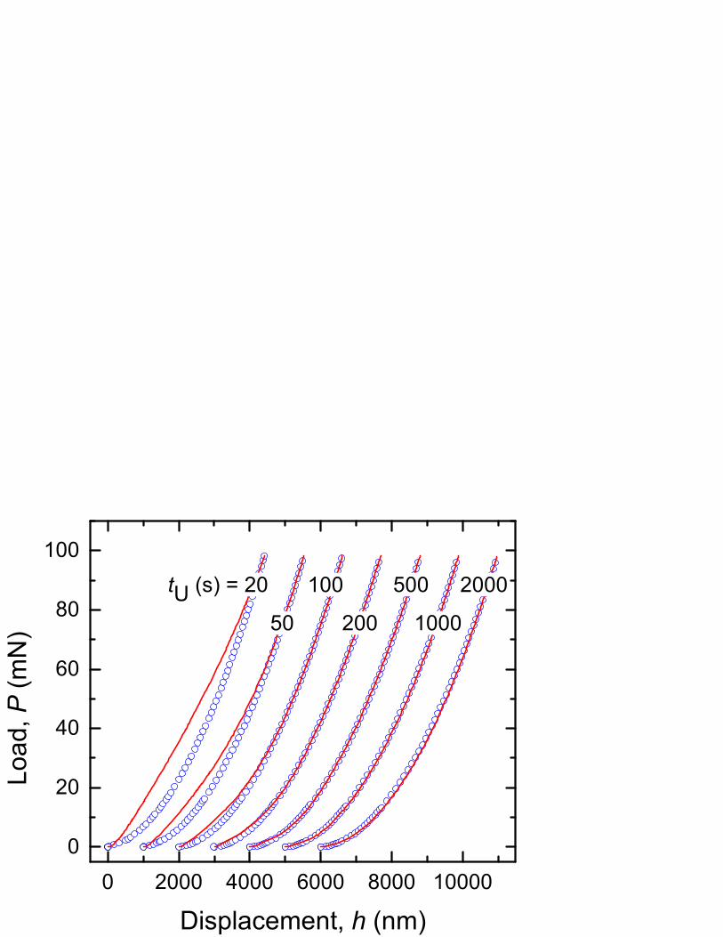
process. Figure 3 shows as symbols the load-displacement behavior of the PMMA1 material

during linear load ramps to 100 mN with rises times from 20 s to 2000 s. (For clarity, as in Figs.

2, 4, and 5, the data are offset and not every measurement is shown.) Inspection of Fig. 3 shows

that that the displacement at peak load increased from about 4000 nm for a rise time of 20 s to

about 5000 nm for a rise time of 2000 s, indicative of greater viscous flow as the test duration

increased over this time scale. The solid lines in Fig. 3 are predictions of the load-displacement

responses using Eq. (10) and the parameters given above. For rise-times comparable to the creep

hold time used to determine the viscoelastic parameters, 1000 s, the predictions are a very good

fit to the measurements. These fits reflect the fact that the 1000 s hold was easily able to capture

the viscoelastic deformation processes associated with the longer τ2 time constant, ≈ 500 s (see

Fig. 2(c)). As the rise times decrease, the predictions do not fit the measurements as well,

particularly in the early part of the experiments. These observations serve to place bounds on the

validity of the model, consistent with the idea that events shorter than about two or three time

constants for a modeled process will not be well described. In this case, the shorter τ1 time

constant places an upper bound on the time scale for events to be well described of ≈ (40 to 60)

s, in agreement with Fig. 3. The obvious remedy, at the cost of model complexity, is to increase

the number of viscoelastic elements and time constants.16,18-20,38 As the inferred properties and

resulting maps here used measurements deliberately not affected by the extreme short rise times

used for illustration in Fig. 3, additional elements were not needed in this study.

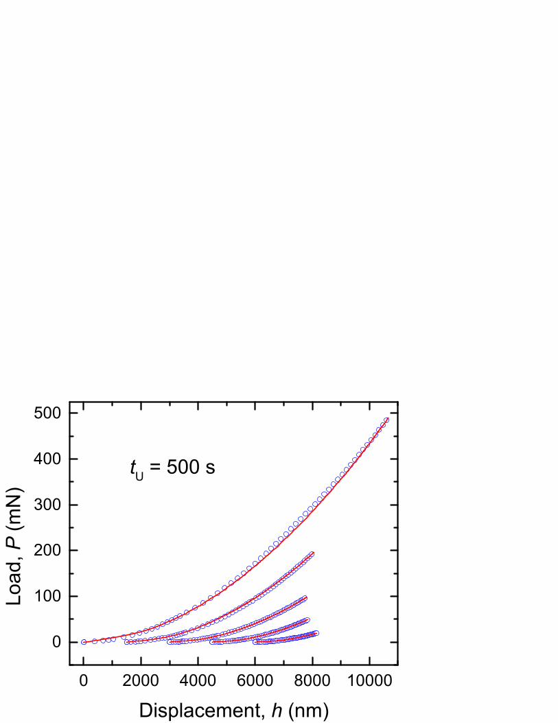
Figure 4 shows as symbols the load-displacement behavior of the PMMA1 material

during linear load ramps to (20 to 500) mN with a rise time of 500 s. The solid lines in Fig. 4 are

predictions of the load-displacement responses using Eq. (10) and the parameters given above. In

distinction to Fig. 3, the predictions are a very good fit to the measurements for all the peak

loads. This latter observation is a consequence of the fact that the relative contributions to total

deformation from plastic and viscoelastic processes remain fixed if the rise time is fixed even as

the peak load (and hence loading rate) changes (Eqs. (9) and (10)). Inserting t = tU into Eq. (10)

gives the displacement hU at peak load of a ramp:

[ ] [ ])/(1)/()/(1)/()/( U22/1

22UU12/1

12U2/1

1UU tfMPtfMPHPh ταταα −+−+= , (10a)

where the functions f are defined by Eqs. (9) or (10) and depend only on the ratio of a material

time constant and the experimental rise time. If the latter is fixed the values of the functions are


fixed and hence the ratio of the first and second terms (the ratio of plastic and viscoelastic

deformation) is also fixed. Eq. (10a) also makes clear that load and loading rate also do not affect

this ratio (providing material properties do not change with load). As the rise time used in Fig. 4

was fixed and long enough to capture the fast and slow viscoelastic processes, the relative

contributions to total displacement and thus the shape of the load-displacement curves remained

invariant; consistent with Eq. (10a), the predictions scaled simply with peak load over the load

range used. (It is possible that plastic deformation will not be initiated or will be suppressed at

very small loads, in which case H would be load-dependent; this was not observed here.)

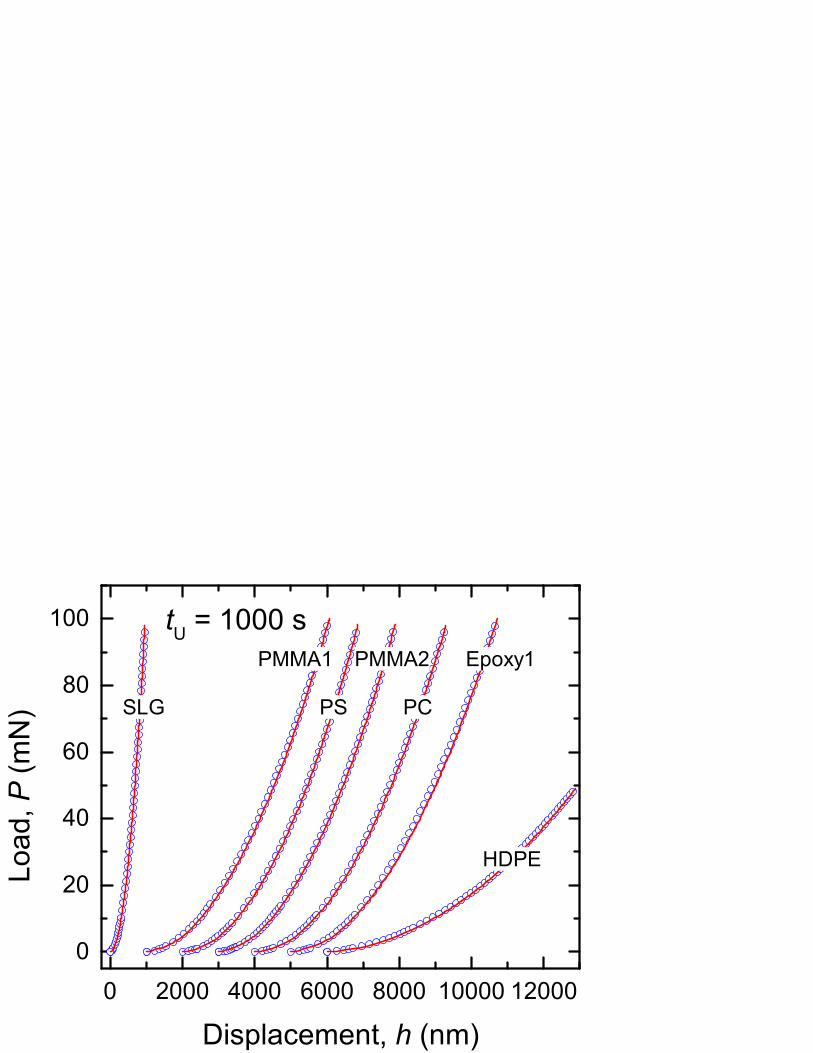
Figure 5 shows as symbols the load-displacement behavior of all the monolithic materials

during linear load ramps with a rise time of 1000 s. The solid lines in Fig. 5 are predictions of the

load-displacement responses using Eq. (10) and the fitted mechanical deformation parameters,

α1H, α2M1, α2M2, τ1, and τ2 for each material. In all cases, the predictions are very good fits to

the measurements. It is clear that SLG is much more resistant and HDPE much less resistant to

indentation deformation under these conditions than the rest of the materials. It is also clear from

the fits in Fig. 5 that the form of the analysis applies to a range of materials that exhibit

viscoelastic and plastic deformation during pyramidal indentation. Comparison of the

magnitudes of the fitted parameters α1H and α2M1 with commonly used values of hardness and

Young’s modulus39,40 for each material suggests that a very good approximation is that α1 and α2

are constants, and that the group of materials is well described by α1 = 100 and α2 = 6. Using

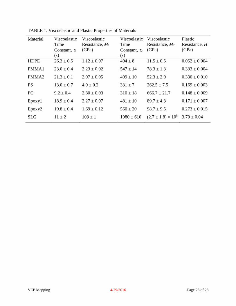
these α parameters, Table 1 gives the values of τ1, M1, τ2, M2, and H determined for each

material, where the values represent the experimental means and standard deviations of best-fit

parameters from four separate experiments. The H values are comparable to those determined

using quasi-static indentation40 and prior VEP methods.1,2,4,7,9,20 The time constants are also

comparable to those observed in indentation measurements in which a two time-constant model

was used: a few tens of seconds for τ1 and a few hundreds of seconds for τ2.3,9,18 The viscoelastic

resistance parameters are comparable to those that can be inferred from a similar study,9 a few

gigapascals for M1 and a few tens of gigapascals for M2, but the comparison is not direct as the

prior study used a slightly different indentation model. A final point of comparison is that for

SLG, which exhibited much greater resistance to viscoelastic deformation than the polymeric

materials but similar time constants, in particular for the fast deformation process characterized


by τ1 = 11 s. Such time dependence is consistent with earlier observations of hysteretic cyclic

indentation of SLG at similar indentation time scales.41,42

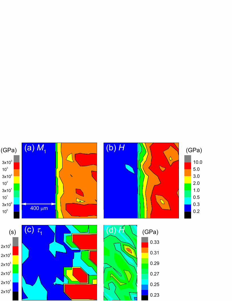
B. Viscoelastic and Plastic Property Mapping Figure 6 shows property maps as color-fill contours over the same area for an extreme

example of a change in properties at the Epoxy 2-AlN interface; the interface is vertical and

located 400 µm from the left edge of the images. To accommodate the extreme range of

properties, Figs. 6(a), (b), and (c) use logarithmic contour intervals. Figure 6(a) is a map of the

viscoelastic resistance parameter M1. At this scale the epoxy appears uniform and is weakly

resistant to viscoelastic deformation. The AlN ceramic is significantly more resistant to

viscoelastic deformation and exhibits some variability in resistance (the weakening adjacent to

the interface reflects the large contour intervals). Figure 6(b) is a similar map of the plastic

resistance H; the appearance is similar to Fig. 6(a). In this extreme example of material changes,

the interface between the epoxy and the ceramic appears sharp in both viscoelastic and plastic

properties maps. Figure 6(c) is a map of the viscoelastic time constant τ1; although the interface

is less distinct, there is still a significant difference between the epoxy and the AlN, and there

appears to be a correlation between M1 and τ1 in the ceramic (in some regions there is more

resistance to viscoelastic deformation and it is slower). Variability in the properties of the epoxy

can be observed by changing the contour scale and this is shown in Fig. 6(d), which is a re-scaled

map of H for the epoxy alone. The epoxy plastic resistance varies by approximately ± 15 %

relatively but there does not seem to be an interface proximity effect as observed in the ceramic,

Fig. 6(b).

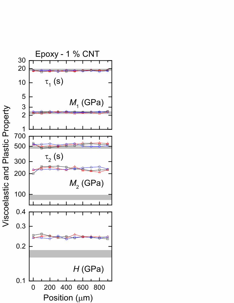
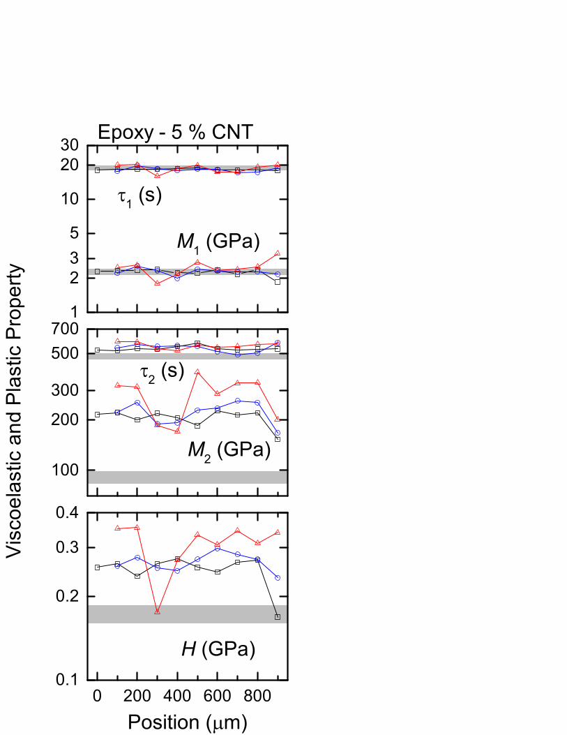
Figures 7 and 8 show the variations in properties along line scans for the 1 % and 5 % CNT

epoxy composites, respectively. The grey bands represent the mean ± two standard deviation

limits (given in Table 1) of the properties determined for Epoxy 1, the composite matrix. The

symbols represent individual measurements in each of three separate scans; different symbols are

used for each scan and the lines are guides to the eye. The composite materials exhibited both

similarities and differences in comparison with the matrix material. For both composites, the

time constants and resistances for the fast viscoelastic process, τ1 and M1, top diagrams, were not

significantly different from those of the matrix. For both composites, the time constants and

resistances for the slow viscoelastic process, τ2 and M2, center diagrams, were significantly


greater than those of the matrix, particularly so for the slow viscoelastic resistance, M2.

Similarly, for both composites, the resistances to plastic deformation, H, bottom diagrams, were

significantly greater than that of the matrix. A significant difference between the composites was

the variability in properties along the line scan. The 5 % composite exhibited much greater

variability in all properties than the 1 % composite, particularly so for M2 and H.

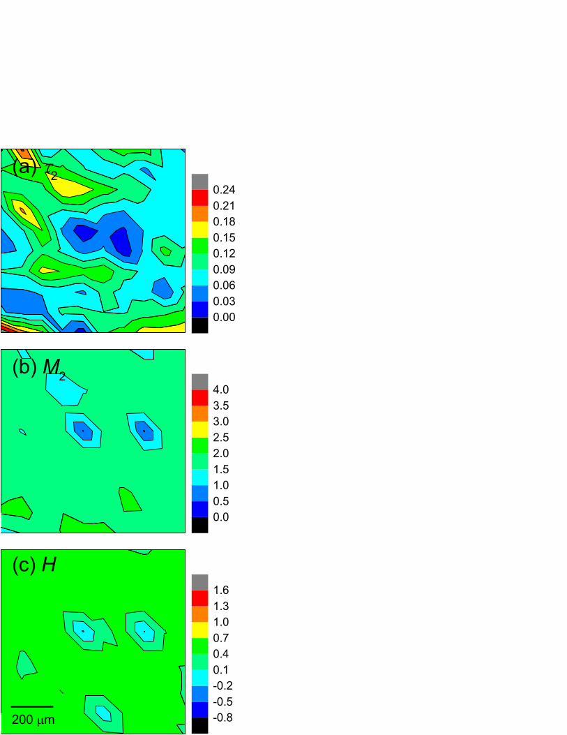
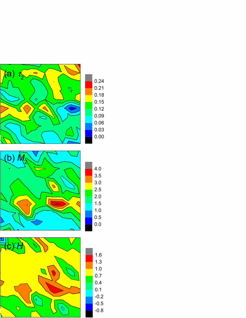
Figures 9 and 10 show property maps for the 1 % and 5 % CNT epoxy composites,

respectively. These maps provide pictorial illustrations of the above similarities and differences,

as well as allowing an assessment of the composite microstructures and the characteristic length

scales for variability or heterogeneity. For ease of comparison, the maps are given as color-filled

contours of relative properties, X*:

matrix

matrixcomposite

XXX

X−

=∗ (11)

such that X* = 0 corresponds to no difference from the matrix; the properties considered were X

= τ2, M2, and H and the same contour intervals were used for each material. Figures 9(a) and

10(a) show maps of the relative time constants ∗2τ for the 1 % and 5 % composites, respectively.

In both cases, the “slow” process in the composite is even slower than in the matrix ( 02 >∗τ ) and

the variability and average of the time constant is greater in the 5% material. Figures 9(b) and

10(b) show maps of the relative viscoelastic resistance ∗2M for the 1 % and 5 % composites. In

both cases, resistance to the slow deformation process is greater than in the matrix, particularly

so for the 5 % material. Finally, Figs. 9(c) and 10(c) show maps of the relative plastic resistance ∗H for the 1 % and 5 % composites. In this case, although the resistance to plastic deformation is

mostly greater than that of the matrix, there are local “soft” spots ( 0<∗H ). The maps of Figs. 9

and 10 are of course consistent with the graphs of Figs. 7 and 8 with regard to values and

variability, but they provide two additional features. The first is that the form and length scales of

the microstructures can easily be observed. The maps suggest that the microstructures are

“clumped” with localized regions that are more resistant to deformation, and that these regions

are approximately 200 µm in size in 1 % material and about 500 µm in size in 5 % material. The

second is that correlations between properties can easily be observed. The maps suggest that

there is a strong correlation between the resistances to viscoelastic and plastic deformation (maps


(b) and (c)) and a weaker correlation between the viscoelastic time constant and resistance (maps

(a) and (b)).

IV. DISCUSSION AND CONCLUSIONS

The results presented here have demonstrated two dimensional mapping of viscoelastic

and plastic properties of polymeric-based materials, extending the mapping capabilities to time-

dependent deformation from those demonstrated previously32-37 using an elastic-plastic

analysis.41 The previous studies all used indentation spacings smaller than the 100 µm used here,

ranging from 0.5 µm32 to 20 µm,35 allowing most maps to be presented with properties as

individual pixels 32,34-36 rather than as contours33,37 as in Figs. 6, 9, and 10. In both the

viscoelastic-plastic mapping here and in the previous elastic-plastic maps the indentation spacing

was matched to the scale of the microstructure and as a consequence there are many similarities

between the previous maps and those obtained here: In previous maps of dense WC

polycrystals,32 tooth enamel,33 lamellar bone,34 quartzite,35 brass,36 and titanium,37 there were

factors of two or three variation in modulus and hardness observed over the maps. These

variations were associated with microstructural variations such as grain orientation or small

variations in composition and are analogous to the variations in properties observed within the

AlN ceramic and epoxy, Fig. 6. In some cases, much greater variations in properties were

observed and were associated with abrupt changes in microstructure, such as decreases of factors

of four in modulus and hardness associated with Co binder in WC-Co composites,32 decreases of

factors of ten associated with graphite flakes in cast iron,36 and much greater decreases

associated with porosity in bone34 and cement.35 These latter variations are analogous to the

variations in properties observed between the AlN and epoxy, Fig. 6.

The above observations and those of prior CNT-epoxy dispersion studies28,31 and reviews29,30

enable interpretation of the line scans and maps of Figs. 7-10 in terms of the CNT composite

microstructures. Figures 7 and 8 show that in both composites the time constant and deformation

resistance of the fast viscoelastic process (τ1, M1) are no different from that of the epoxy matrix.

This observation suggests that the CNTs do not influence this deformation mechanism at all and

that it is entirely associated with the epoxy and probably molecular in scale. Conversely, Figs. 7

and 8 show that for the slow viscoelastic process (τ2, M2) in both composites the time constant is


increased somewhat and the deformation resistance is increased substantially from that of the

epoxy. The implication here is that the incorporated CNTs are slowing this deformation process

and making it more difficult, probably over length scales comparable to the indentation size,

about 5 µm (Fig. 5). Figures 7 and 8 also show that the resistance to plastic deformation, H, is

increased substantially from that of the epoxy for both composites, consistent with the idea that

the CNTs impeded both slow, time-dependent- and irreversible, time-independent-deformation

on length scales comparable to the indentation field. Figures 9 and 10 highlight, however, that

the increases in M2 and H are not uniform: some areas exhibit less than average deformation

resistance, e.g., in Fig. 9, and some areas exhibit greater than average deformation resistance,

e.g., in Fig. 10, with strong correlation between M2 and H. These areas probably reflect localized

increased concentrations of CNTs and are comparable in size to the hundreds of micrometer-31 to

millimeter-scale28 agglomerates observed previously. Removal of such entangled agglomerates is

a major focus of the many methods29,30 used to disperse CNTs in polymer matrices, as the

agglomerates are only weakly infiltrated by the polymer and thereby degrade the composite

properties relative to those that might be achieved by well-dispersed CNTs bound to the matrix.

This degradation is probably the case in Fig. 9, which shows local “soft” spots. Counter to this is

Fig. 10, which shows local “hard” spots possibly reflecting enhanced areas of CNT concentration

with adequate polymer infiltration. The advantage of maps such as Figs. 9 and 10 is that local

variations in properties are assessed directly and do not have to be inferred from measurements

of entire composite components.31 An implication from Figs. 7-10 is that the CNTs in the 5%

material were less uniformly dispersed than in the 1 % material. Imaging spectroscopy methods,

e.g., Raman spectroscopy as applied to single-wall CNT composites,43 could possibly be used to

directly assess CNT dispersion for comparison with the mechanical measurements.

Application of the method developed here to prediction of properties for a particular

material requires a few additional steps. First, to establish accuracy (how close a measurement

represents a true or known value), independent measurements of properties should be performed

so as to fix the geometry terms α1 and α2 for the materials class under consideration. The

material-invariant approximation used here returns reasonable property values (section III.A and

Table 1) for a range of materials, but does not necessarily apply in detail to a specific material.

Such independent measurements should be viscoelastic experiments, noting that the M values

used here are viscoelastic resistances and include elastic moduli as lower bounds. Second, to


establish precision (how close a measurement represents a mean value) sufficient measurements

should be performed to place statistical bounds on the determined τ1, M1, τ2, M2, and H

parameters. Table 1 suggests that four measurements provides sufficient precision for

homogeneous materials at the indentation scale used here, but indentations at smaller scales,

particularly in materials with heterogeneous microstructures, will lead to less precision (e.g., as

in the elastic-plastic indentation studies above32,36,37) and require greater numbers of

indentations. This last point pertains particularly to composite materials: If globally averaged

properties are required for a composite, say to predict the overall response of a component,

sufficient numbers of indentations over a large enough area are required so as to assess the

characteristic length scales of the microstructure. This in turn sets the “representative volume

element” for the material that is the minimum component scale that can be regarded as

possessing average properties. Third, in order to validate the assumed constitutive law and

measured deformation parameters, predictions should be made and tested against loading

protocols close to those expected in component operation, or at least different from those used to

determine the parameters. Here, predictions from the three-segment measurements (Fig. 2) were

tested against ramp loading protocols (Figs. 3-5) for which closed-form solutions (Eq. (10)) were

developed. Similar validations are often performed,1,2,4,8,18-20 but often not, especially when

viscoelastic correspondence methods are used to analyze measurements.3,9,12,13,16,17 In this regard,

it is to be noted that for non-simple loading protocols or those with multiple stages, the integrand

of the general displacement integral (Eq. (A5)) will usually not be too pathological and therefore

amenable to straightforward numerical integration. It is also to be noted that the viscoelastic

correspondence methods23-27 do not allow for unloading of the indenter (formally, they only

allow monotonically increasing contact radius), which is not an inherent limitation of the VEP

approach and which can be tested experimentally.4,9,12 Extension to arbitrary, multiple-stage

loading protocols including unloading and numerical prediction of load-displacement-time

responses will be the subject of future work.

Finally, practical considerations for indentation-based mapping of the mechanical

properties of polymeric systems are that time will nearly always be an inherent part of the

measurement procedure and that the indentations will invariably be large. Hence, maps that

involve viscoelastic properties will always take longer to generate than those that only involve

elastic-plastic properties, and maps of “soft” materials will always require indentation spacing


greater than that of hard materials. As noted above, matching the indentation spacing and size to

the length scale of the microstructure is important such that maps do not over- or under-sample.

In polymeric composite systems with microstructural scales smaller than that examined here,

finely spaced line scans about three indentation dimensions apart might provide a compromise

between generating an accurate assessment of the heterogeneity of time-dependent mechanical

responses and maintaining reasonable test durations.

ACKNOWLEDGMENTS

This research was performed while AJG was initially an undergraduate student volunteer

researcher at NIST and subsequently a member of the NIST Summer Undergraduate Research

Fellowship (SURF) program. The authors thank APV Engineered Coatings and Arkema for

assistance with sample preparation and Drs. Doug Smith and Brian Bush of NIST for

experimental assistance. Certain commercial equipment, instruments or materials are identified

in this document. Such identification does not imply recommendation or endorsement by the

National Institute of Standards and Technology, nor does it imply that the products identified are

necessarily the best available for the purpose.


REFERENCES 1. M.L. Oyen and R.F. Cook: Load–displacement behavior during sharp indentation of

viscous–elastic–plastic materials. J. Mater. Res. 18, 139 (2003).

2. M.L. Oyen, R.F. Cook, J.A. Emerson, and N.R. Moody: Indentation responses of time-

dependent films on stiff substrates. J. Mater. Res. 19, 2487 (2004).

3. C.Y. Zhang, Y.W. Zhang, K.Y. Zeng, and L. Shen: Nanoindentation of polymers with a

sharp indenter. J. Mater. Res. 20, 1597 (2005).

4. R.F. Cook and M.L. Oyen: Nanoindentation behavior and mechanical properties

measurement of polymeric materials. Int. J. Mater. Res. 98, 370 (2007).

5. M.L. Oyen and C.-C. Ko: Examination of local variations in viscous, elastic, and plastic

indentation responses in healing bone. J. Mater. Sci: Mater. Med. 18, 623 (2007).

6. M.L. Oyen and R.F. Cook: A practical guide for analysis of nanoindentation data. J. Mech.

Behavior Biomedical Mater. 2, 396 (2009).

7. S.E. Olesiak, M.L. Oyen, and V.L. Ferguson: Viscous-elastic-plastic behavior of bone

using Berkovich nanoindentation. Mech. Time-Depend. Mater. 14, 111 (2010).

8. Y. Wang and I.K. Lloyd: Time-dependent nanoindentation behavior of high elastic

modulus dental resin composites. J. Mater. Res. 25, 529 (2010).

9. P.-E. Mazeran, M. Beyaoui, M. Bigerelle, and M. Guigon: Determination of mechanical

properties by nanoindentation in the case of viscous materials. Int. J. Mater. Res. 103, 715

(2012).

10. M. Sakai, S. Kawaguchi, and N. Hakiri: Contact-area-based FEA study on conical

indentation problems for elastoplastic and viscoelastic-plastic bodies. J. Mater. Res. 27,

256 (2012).

11. N. Rodriguez-Florez, M.L. Oyen, and S.J. Shefelbine: Insight into differences in

nanoindentation properties of bone. J. Mech. Behavior Biomedical Mater. 18, 90 (2013).

12. S.J. Isaza, P.-E. Mazeran, K. El Kirat, and M.-C. Ho Ba Tho: Time-dependent mechanical

properties of rat femoral cortical bone by nanoindentation: An age-related study. J. Mater.

Res. 29, 1135 (2014).

13. L. Cheng, X. Xia, W. Yu, L.E. Scriven, and W.W. Gerberich: Flat-Punch Indentation of

Viscoelastic Material. J. Polym. Sci.: Part B: Polym. Phys. 38, 10 (2000).


14. M. Sakai and S. Shimizu: Indentation rheometry for glass-forming materials. J. Non-Cryst.

Solids 282, 236 (2001).

15. M. Sakai: Time-dependent viscoelastic relation between load and penetration for an

axisymmetric indenter. Phil. Mag. A 82, 1841 (2002).

16. S. Yang, Y.-W. Zhang, and K. Zeng: Analysis of nanoindentation creep for polymeric

materials. J. Appl. Phys. 95, 3655 (2004).

17. L. Cheng, X. Xia, L.E. Scriven, and W.W. Gerberich: Spherical-tip indentation of

viscoelastic material. Mech. of Mater. 37, 213 (2005).

18. M.L. Oyen: Spherical indentation creep following ramp loading. J. Mater. Res. 20, 2094

(2005).

19. J. M. Mattice, A.G. Lau, M.L. Oyen, and R.W. Kent: Spherical indentation load-relaxation

of soft biological tissues. J. Mater. Res. 21, 2003 (2006).

20. M.L. Oyen: Analytical techniques for indentation of viscoelastic materials. Phil. Mag. 86,

5625 (2006).

21. S. Shimizu, T. Yanagimoto, and M. Sakai: Pyramidal indentation load-depth curve of

viscoelastic materials. J. Mater. Res. 14, 4075 (1999).

22. M. Sakai, S. Shimizu, N. Miyajima, Y. Tanabe, and E. Yasuda: Viscoelastic indentation of

iodine-treated coal tar pitch. Carbon 39, 605 (2001).

23. E.H. Lee and J.R.M. Radok: The Contact Problem for Viscoelastic Bodies. J. Appl. Mech.

27, 438 (1960).

24. S.C. Hunter: The Hertz Problem for a Rigid Spherical Indenter and a Viscoelastic Half-

Space. J. Mech. Phys. Solids 8, 219 (1960).

25. G.A.C. Graham: The Contact Problem in the Linear Theory of Viscoelasticity. Int. J.

Engng Sci. 3, 27 (1965).

26. W.H. Yang: The Contact Problem for Viscoelastic Bodies. J. Appl. Mech. 32, 395 (1966).

27. T.C.T. Ting: The Contact Stresses between a Rigid Indenter and a Viscoelastic Half-Space.

J. Appl. Mech. 33, 845 (1966).

28. J. Sandler, M.S.P. Shaffer, T. Prasse, W. Bauhofer, K. Schulte, and A.H. Windle:

Development of a dispersion process for carbon nanotubes in an epoxy matrix and the

resulting electrical properties. Polymer 40, 5967 (1999).


29. X.-L. Xie, Y.-W. Mai, and X.-P. Zhou: Dispersion and alignment of carbon nanotubes in

polymer matrix: A review. Mater. Sci. Eng. R 49, 89 (2005).

30. P.-C. Ma, N.A. Siddiqui, G. Marom, and J.-K. Kim: Dispersion and functionalization of

carbon nanotubes for polymer-based nanocomposites: A review. Composites: Part A 41,

1345 (2010).

31. A.K. Chakraborty, T. Plyhm, M. Barbezat, A. Necola, and G.P. Terrasi: Carbon nanotube

(CNT)–epoxy nanocomposites: a systematic investigation of CNT dispersion. J. Nanopart.

Res. 13, 6493 (2011).

32. H. Engqvist and U. Wiklund: Mapping of mechanical properties of WC–Co using

nanoindentation. Trib. Letters 8, 147 (2000).

33. J.L. Cuy, A.B. Mann, K.J. Livi, M.F. Teaford, and T.P. Weihs: Nanoindentation mapping

of the mechanical properties of human molar tooth enamel. Arch. Oral Biol. 47, 281

(2002).

34. H.S. Gupta, U. Stachewicz, W. Wagermaier, P. Roschger, H.D. Wagner, and P. Fratzl:

Mechanical modulation at the lamellar level in osteonal bone. J. Mater. Res. 21, 1913

(2006).

35. W. Zhu, J.J. Hughes, N. Bicanic, and C.J. Pearce: Nanoindentation mapping of mechanical

properties of cement paste and natural rocks. Mater. Charact. 58, 1189 (2007).

36. N.X. Randall, M. Vandamme, and F.-J. Ulm: Nanoindentation analysis as a two-

dimensional tool for mapping the mechanical properties of complex surfaces. J. Mater.

Res. 24, 679 (2009).

37. D. Goldbaum, R.R. Chromik, N. Brodusch, and R. Gauvin: Microstructure and Mechanical

Properties of Ti Cold-Spray Splats Determined by Electron Channeling Contrast Imaging

and Nanoindentation Mapping. Microsc. Microanal. 21, 570 (2015).

38. W.N. Findley, J.S. Lai, and K. Onaran: Creep and Relaxation of Nonlinear Viscoelastic

Materials (Dover Publications, Inc., New York, 1989).

39. W.D. Callister: Materials Science and Engineering (John Wiley & Sons, Inc., New York,

1997).

40. CES Selector Version 4.5 (Granta Design Limited, Cambridge, UK, 2004).


41. W.C. Oliver and G.M. Pharr: An improved technique for determining hardness and elastic

modulus using load and displacement sensing indentation experiments. J. Mater. Res. 7,

1564 (1992).

42. J. Thurn and R.F. Cook: Indentation-induced deformation at ultramicroscopic and

macroscopic contacts. J. Mater. Res. 19, 124 (2004).

43. F. Du, R.C. Scogna, W. Zhou, S. Brand, J.E. Fischer, and K.I. Winey: Nanotube Networks

in Polymer Nanocomposites: Rheology and Electrical Conductivity. Macromolecules 37,

9048 (2004).

44. Wolfram Mathematica, http://integrals.wolfram.com (accessed 8/14/14).

http://integrals.wolfram.com/


TABLE 1. Viscoelastic and Plastic Properties of Materials

Material Viscoelastic Time Constant, τ1 (s)

Viscoelastic Resistance, M1 (GPa)

Viscoelastic Time Constant, τ2 (s)

Viscoelastic Resistance, M2 (GPa)

Plastic Resistance, H (GPa)

HDPE 26.3 ± 0.5 1.12 ± 0.07 494 ± 8 11.5 ± 0.5 0.052 ± 0.004

PMMA1 23.0 ± 0.4 2.23 ± 0.02 547 ± 14 78.3 ± 1.3 0.333 ± 0.004

PMMA2 21.3 ± 0.1 2.07 ± 0.05 499 ± 10 52.3 ± 2.0 0.330 ± 0.010

PS 13.0 ± 0.7 4.0 ± 0.2 331 ± 7 262.5 ± 7.5 0.169 ± 0.003

PC 9.2 ± 0.4 2.80 ± 0.03 310 ± 18 666.7 ± 21.7 0.148 ± 0.009

Epoxy1 18.9 ± 0.4 2.27 ± 0.07 481 ± 10 89.7 ± 4.3 0.171 ± 0.007

Epoxy2 19.8 ± 0.4 1.69 ± 0.12 560 ± 20 98.7 ± 9.5 0.273 ± 0.015

SLG 11 ± 2 103 ± 1 1080 ± 610 (2.7 ± 1.8) × 105 3.70 ± 0.04


APPENDIX: VEP Model Development The starting point for the quadratic viscoelastic Kelvin element is the linear Kelvin

element load-displacement function:38

thkhP

ddη+= , (A1)

where k is interpreted as a stiffness, η is interpreted as a viscosity, and the load is interpreted as

the sum of the loads supported by an elastic element (k) and a viscous element (η) in parallel.

Equation (A1) can be re-written as

+=

thhP

dd

τη , (A2a)

where

kητ = (A2b)

is a characteristic time constant. By analogy with the quadratic viscous element described by Eq.

(3), the quadratic viscoelastic Kelvin element is described by squaring the right side of Eq.

(A2a),

2

22 d

d

+=

thhMP

ττα , (A3)

where the term α2Mτ2 is here an effective or lumped quadratic viscoelastic resistance. The first

term in the parentheses in Eq. (A3) represents the elastic contribution to the resistance and the

second term the viscous contribution. Inverting Eq. (A3) leads to a differential equation for the

viscoelastic displacement resulting from an imposed load spectrum:

2/1

2

)(1dd

=+

MtPh

th

αττ. (A4)

This is a differential equation of the form

QhRh =+

with R and Q defined by Eq. (A4) that can be solved with use of an integrating factor

( )

)/exp(

dexp

τ

ρ

t

tR

=

= ∫ ,

with solution


CtQh += ∫ dρρ ,

where C is a constant of integration. Hence, the viscoelastic displacement can be written as

ττ

τ

ατ/

2/1

2

// d)( t

tt Cet

MtPeeh −− +

= ∫ . (A5)

The time spectra of interest here are linear, of the form

P(t) = A + Bt. (A6)

In particular, for a ramp load from zero to a peak of PR in a time of tR, A = 0 and B = PR/tR in Eq.

(A6), and the solution to Eq. (A5) is, using Mathematica,44

ττττπ /2/12/12/1 ])/[(erfi)/exp()(2

)( tCettbbth −+−−= (A7a)

where

MtPb

2R

R

α= . (A7b)

The function erfi(z) is the complex error function given by erfi(z) = −ierf(z), where erf(z) is the

general error function, z is complex, and i2 = −1. It is easy to show that if the argument z = x is

real that erfi(x) = erf(x). This is case here, Eq. (A7a), such that

R2/12/12/1 ,)/(erf)/exp()(

2)( ttttbbth ≤−−= τττπ (A8)

using h = 0 at t = 0 to show that C = 0, and where the notation for erf(x)1/2 in Eq. (A8) follows

directly from Eq. (A7a). The first term on the right side of Eq. (A8) represents the displacement

of a free elastic element and the second term represents the modification by the viscous element.

Setting t = tR in Eq. (A8) gives h(tR) = hR, the viscoelastic displacement at the peak of the ramp

load.

For a load hold at the peak value, after a ramp, A = PR and B = 0 in Eq. (A6), and the

solution to Eq. (A5) is, using separation of variables,

[ ] RR

R2/1

R ,)(exp1 tttthahh ≥

−−−−+=

τ, (A9a)

where

M

Pa2

R

α= . (A9b)


The term hR appears in both additive and multiplicative roles on the right side of Eq. (A9a),

modifying the creep response (Eq. (A9)) by displacement accrued during the prior ramp (Eq.

(A8)). In this sense, hR acts as a “ramp correction factor” used earlier in a linear viscoelastic

context.18,19 Equation (A9) contains an essential result of the analysis: For (t − tR) >> τ the creep

displacement approaches a bounded value of 2/12R )/( MPh α→ in a non-linear manner.

Alternatively, for a ramp unload from the peak of PR to zero in a time of tR, A = 2PR and

B = −PR/tR in Eq. (A6), and the solution to Eq. (A5) is, using Mathematica,44

+

+

+

+

−+=τττ

τπb

btahb

btab

btabbtah experfexp)(2

)( F

2/12/12/1 , (A10a)

RR 2ttt ≤≤ ,

where now

MPa2

R2α

= , Mt

Pb2R

R

α−= . (A10b)

Setting t = 2tR in Eq. (A10) gives h(2tR) = hF, the displacement at the end of the triangular load

spectrum. Noting that both Eqs. (A8) and (A10) must pertain at t = tR, hF can be determined in

terms of hR and thus in terms of test and material parameters.

Combining Eqs. (A8) and (A10) generates load-displacement responses that are

indistinguishable from those observed in experiments and determined using the earlier Maxwell-

like VEP model during triangle-wave loading.1,4 In particular, for slow tests the current model

exhibits the initial negative unloading slope and unloading “nose.” The explicit behavior

described by Eq. (A10) will not be used here, but it is noted that in a zero-load recovery segment

after a triangular load spectrum, such that A = B = 0, the viscoelastic displacement is given by

the last term in Eq. (A5) alone, such that

RR

F 2,)2(exp tttthh ≥

−−=

τ, (A11)

Equation (A11) contains another essential result of the analysis: For (t − 2tR) >> τ in a recovery

segment, the viscoelastic displacement 0→h in a non-linear manner.


Figure Captions

FIG.1. Schematic diagram of the pyramidal indentation quadratic Kelvin viscous elastic plastic

model. The model consists of two quadratic viscoelastic Kelvin elements in series with a

quadratic plastic element.

FIG. 2. Experimental load-displacement-time, P-h-t, data for the PMMA1 material during the

three-segment indentation test. (a) The imposed triangle-hold-trapezoid load spectrum; the end of

the initial triangle to peak load PT and the beginning of the creep segment at load PR of the final

trapezoid are indicated by vertical lines. (b) The resulting displacement response; at the end of

the central hold the displacement is hPT. (c) The displacement in the creep segment of the final

trapezoid in shifted coordinates.

FIG. 3. Load-displacement responses of the PMMA1 material during linear load-time

indentation ramps to the same peak load, but different rise times, tU. Symbols indicate

experimental observations (not all shown) and the lines indicate predictions from measurements

and analyses of three segment (Fig. 2) tests. Data offset horizontally for clarity.

FIG. 4. Load-displacement responses of the PMMA1 material during linear load-time

indentation ramps with the same rise time, but different peak loads. Symbols indicate

experimental observations (not all shown) and the lines indicate predictions from measurements

and analyses of three segment (Fig. 2) tests. Data offset horizontally for clarity.

FIG. 5. Load-displacement responses of silicate glass and polymer materials during linear load-

time indentation ramps. Symbols indicate experimental observations (not all shown) and the

lines indicate predictions from measurements and analyses of three segment (Fig. 2) tests. Data

offset horizontally for clarity.

FIG. 6. Color-fill contour maps of mechanical properties variations at an epoxy-AlN interface;

the epoxy extends 400 µm from the left of the maps as indicated by the arrow. (a) The resistance

to viscoelastic deformation, M1, for the fast process in the epoxy. (b) The resistance to plastic

deformation, H. (c) The viscoelastic deformation time constant, τ1, for the fast process. (d) The

resistance to plastic deformation, H, in the epoxy, re-scaled to enhance variation.

FIG. 7. Variations in mechanical properties of 1 % CNT-epoxy composite along line scans. The

grey bands indicate the properties of the epoxy matrix. (Upper) Time constant and resistance to


deformation for the fast viscoelastic deformation process, (τ1, M1). (Central) Time constant and

resistance to deformation for the slow viscoelastic deformation process, (τ2, M2). (Lower)

Resistance to plastic deformation, H.

FIG. 8. Variations in mechanical properties of 5 % CNT-epoxy composite along line scans.

Notation as in Fig. 7.

FIG. 9. Color-fill contour maps of mechanical properties variations in 1 % CNT-epoxy

composite. The properties are plotted relative to the epoxy matrix using Eq. (11). (a) The

viscoelastic time constant, τ2, for the slow deformation process. (b) The resistance to viscoelastic

deformation, M2, for the slow process. (c) The resistance to plastic deformation, H.

FIG. 10. Color-fill contour maps of mechanical properties variations in 5 % CNT-epoxy

composite. Notation as in Fig. 9.

Date post:	31-Dec-2021
Category:	Documents
Upload:	others
View:	1 times
Download:	0 times

Mapping Viscoelastic and Plastic Properties of Polymers ...

Documents