49
MapReduce Algorithms CSE 490H
| Date post: | 20-Dec-2015 |
| Category: |
Documents |
| View: | 236 times |
| Download: | 1 times |

MapReduce Algorithms
CSE 490H
Algorithms for MapReduce
Sorting Searching TF-IDF BFS PageRank More advanced algorithms
MapReduce Jobs
Tend to be very short, code-wise IdentityReducer is very common
“Utility” jobs can be composed Represent a data flow, more so than a
procedure
Sort: Inputs
A set of files, one value per line. Mapper key is file name, line number Mapper value is the contents of the line
Sort Algorithm
Takes advantage of reducer properties: (key, value) pairs are processed in order by key; reducers are themselves ordered
Mapper: Identity function for value(k, v) (v, _)
Reducer: Identity function (k’, _) -> (k’, “”)
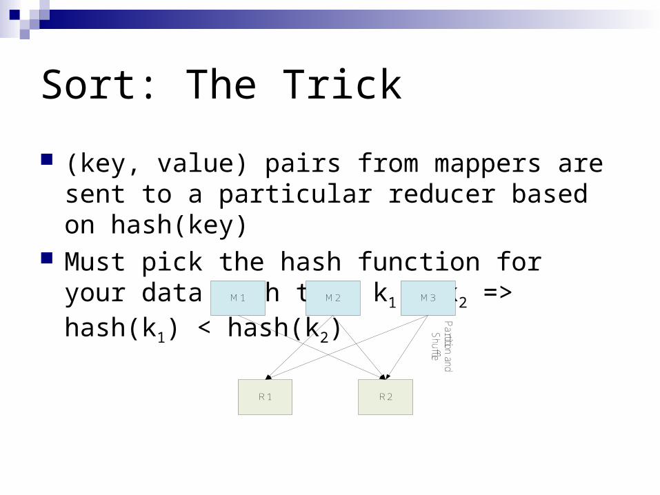
Sort: The Trick
(key, value) pairs from mappers are sent to a particular reducer based on hash(key)
Must pick the hash function for your data such that k1 < k2 => hash(k1) < hash(k2)
M1 M2 M3
R1 R2
Partition and
Shuffle
Final Thoughts on Sort
Used as a test of Hadoop’s raw speed Essentially “IO drag race” Highlights utility of GFS
Search: Inputs
A set of files containing lines of text A search pattern to find
Mapper key is file name, line number Mapper value is the contents of the line Search pattern sent as special parameter
Search Algorithm
Mapper:Given (filename, some text) and “pattern”, if
“text” matches “pattern” output (filename, _) Reducer:
Identity function
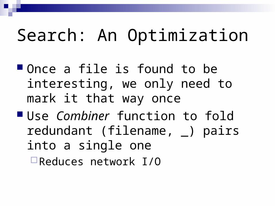
Search: An Optimization
Once a file is found to be interesting, we only need to mark it that way once
Use Combiner function to fold redundant (filename, _) pairs into a single oneReduces network I/O
TF-IDF
Term Frequency – Inverse Document FrequencyRelevant to text processingCommon web analysis algorithm
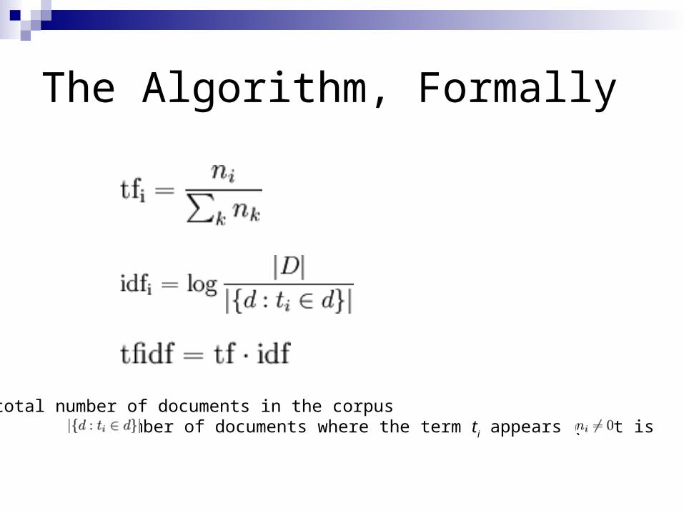
The Algorithm, Formally
•| D | : total number of documents in the corpus • : number of documents where the term ti appears (that is ).
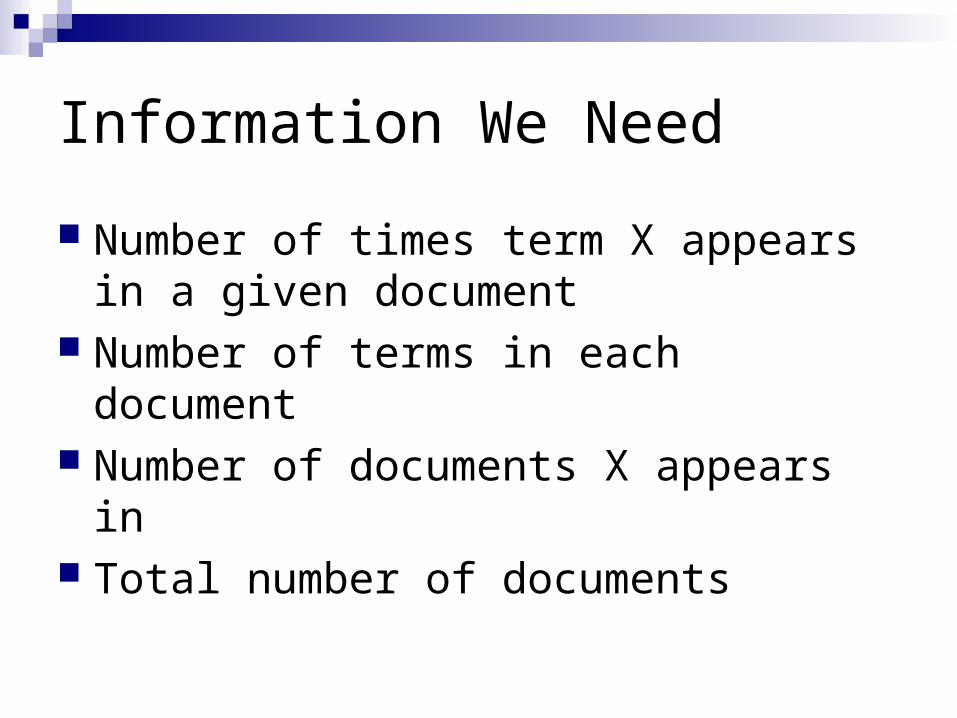
Information We Need
Number of times term X appears in a given document
Number of terms in each document Number of documents X appears in Total number of documents
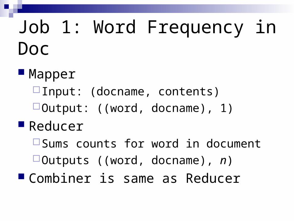
Job 1: Word Frequency in Doc
Mapper Input: (docname, contents)Output: ((word, docname), 1)
ReducerSums counts for word in documentOutputs ((word, docname), n)
Combiner is same as Reducer
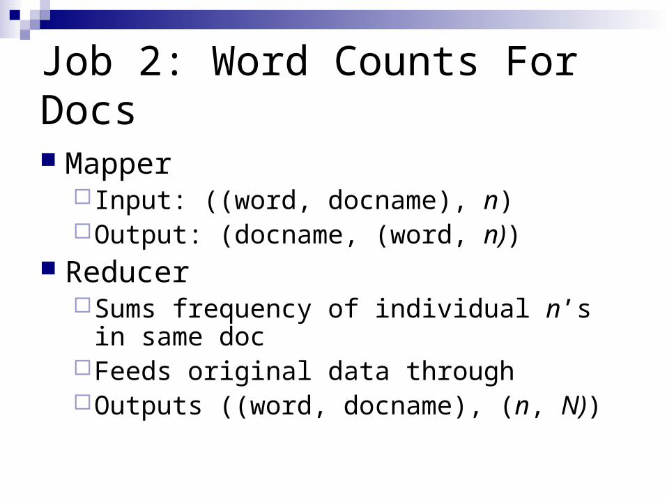
Job 2: Word Counts For Docs
Mapper Input: ((word, docname), n)Output: (docname, (word, n))
ReducerSums frequency of individual n’s in same docFeeds original data throughOutputs ((word, docname), (n, N))
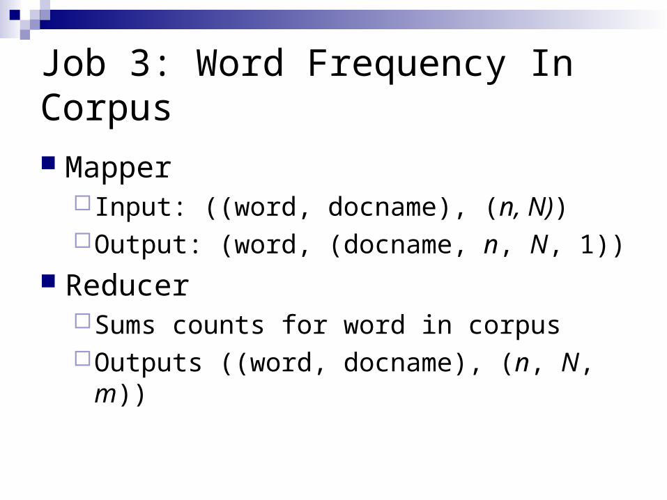
Job 3: Word Frequency In Corpus
Mapper Input: ((word, docname), (n, N))Output: (word, (docname, n, N, 1))
ReducerSums counts for word in corpusOutputs ((word, docname), (n, N, m))
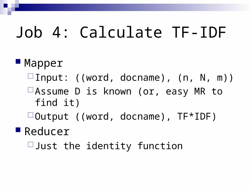
Job 4: Calculate TF-IDF
Mapper Input: ((word, docname), (n, N, m))Assume D is known (or, easy MR to find it)Output ((word, docname), TF*IDF)
ReducerJust the identity function
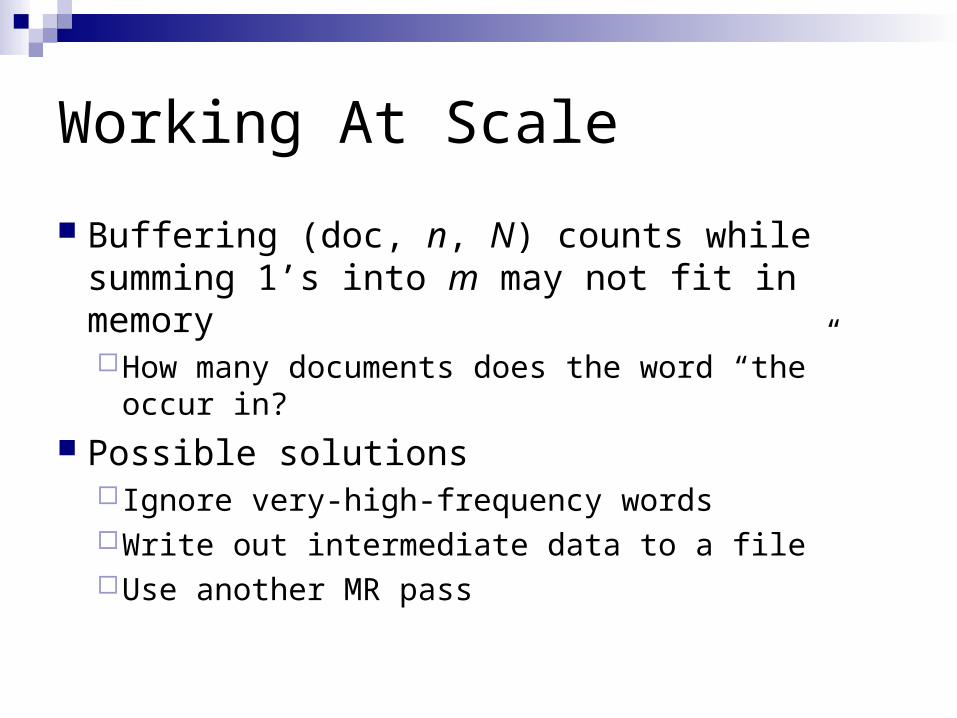
Working At Scale
Buffering (doc, n, N) counts while summing 1’s into m may not fit in memoryHow many documents does the word “the”
occur in? Possible solutions
Ignore very-high-frequency wordsWrite out intermediate data to a fileUse another MR pass
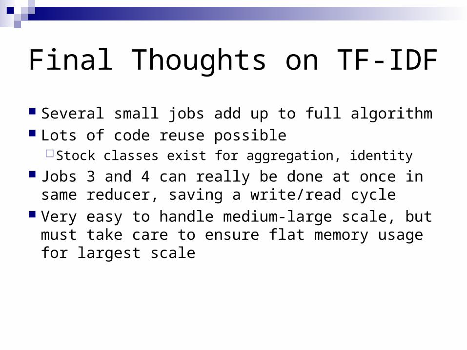
Final Thoughts on TF-IDF
Several small jobs add up to full algorithm Lots of code reuse possible
Stock classes exist for aggregation, identity Jobs 3 and 4 can really be done at once in
same reducer, saving a write/read cycle Very easy to handle medium-large scale, but
must take care to ensure flat memory usage for largest scale
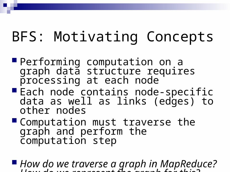
BFS: Motivating Concepts
Performing computation on a graph data structure requires processing at each node
Each node contains node-specific data as well as links (edges) to other nodes
Computation must traverse the graph and perform the computation step
How do we traverse a graph in MapReduce? How do we represent the graph for this?
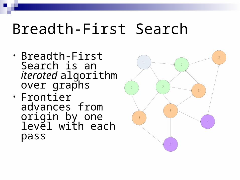
Breadth-First Search
• Breadth-First Search is an iterated algorithm over graphs
• Frontier advances from origin by one level with each pass
12
2 2
3
3
3
3
4
4
Breadth-First Search & MapReduce
Problem: This doesn't “fit” into MapReduce Solution: Iterated passes through
MapReduce – map some nodes, result includes additional nodes which are fed into successive MapReduce passes
Breadth-First Search & MapReduce
Problem: Sending the entire graph to a map task (or hundreds/thousands of map tasks) involves an enormous amount of memory
Solution: Carefully consider how we represent graphs
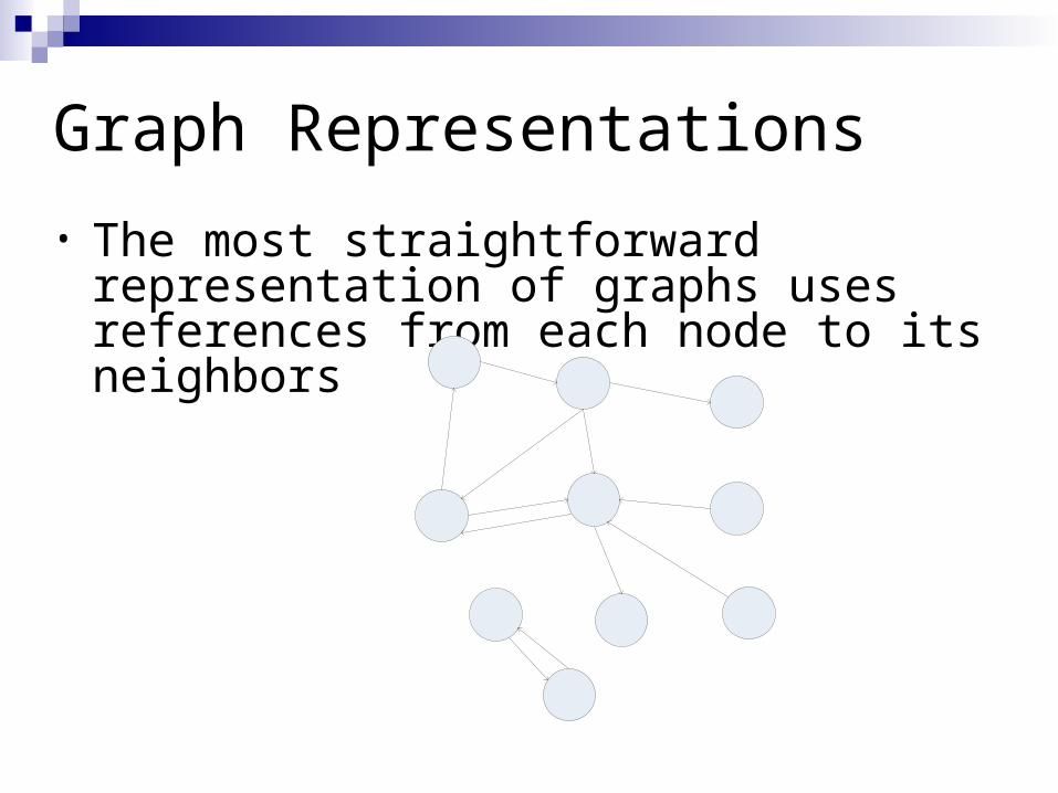
Graph Representations
• The most straightforward representation of graphs uses references from each node to its neighbors
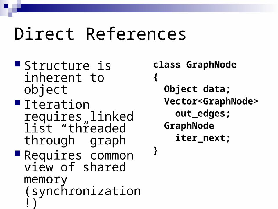
Direct References
Structure is inherent to object
Iteration requires linked list “threaded through” graph
Requires common view of shared memory (synchronization!)
Not easily serializable
class GraphNode{ Object data; Vector<GraphNode> out_edges; GraphNode iter_next;}
Adjacency Matrices
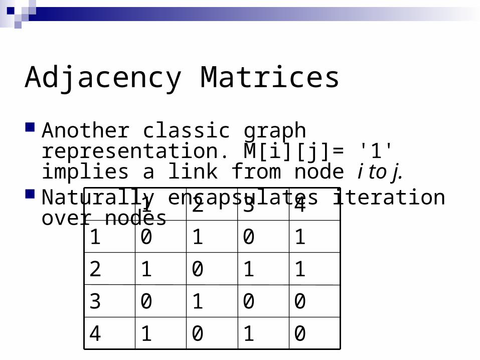
Another classic graph representation. M[i][j]= '1' implies a link from node i to j.
Naturally encapsulates iteration over nodes
01014
00103
11012
10101
4321
Adjacency Matrices: Sparse Representation
Adjacency matrix for most large graphs (e.g., the web) will be overwhelmingly full of zeros.
Each row of the graph is absurdly long
Sparse matrices only include non-zero elements
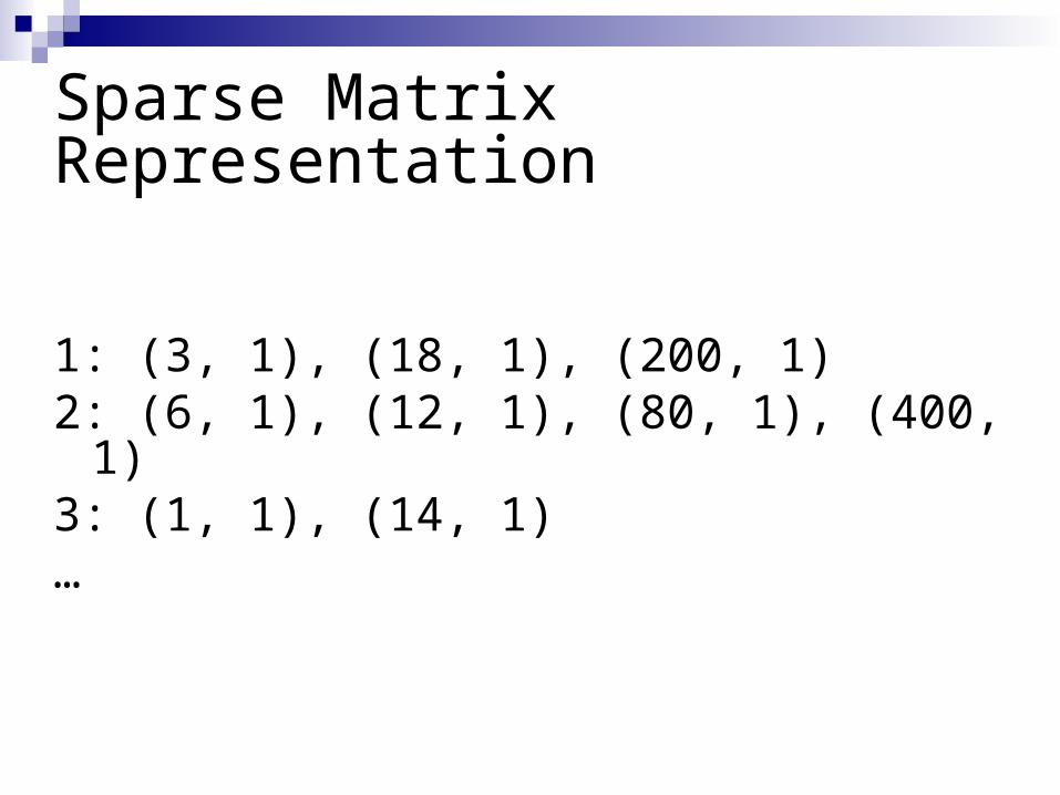
Sparse Matrix Representation
1: (3, 1), (18, 1), (200, 1)2: (6, 1), (12, 1), (80, 1), (400, 1)3: (1, 1), (14, 1)…
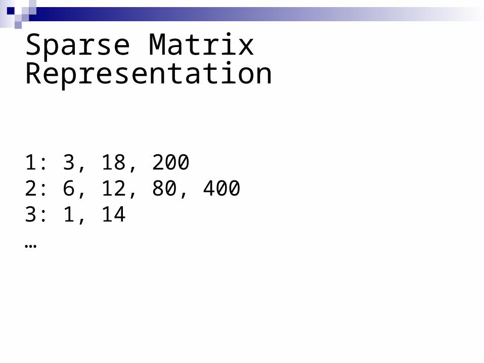
Sparse Matrix Representation
1: 3, 18, 2002: 6, 12, 80, 4003: 1, 14…
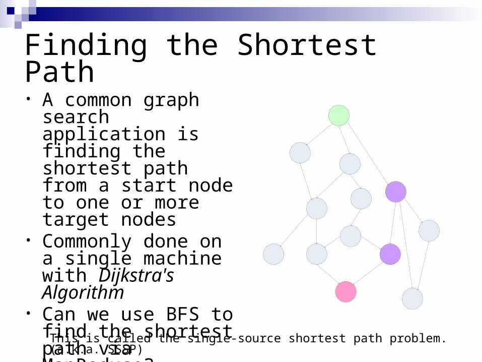
Finding the Shortest Path• A common graph
search application is finding the shortest path from a start node to one or more target nodes
• Commonly done on a single machine with Dijkstra's Algorithm
• Can we use BFS to find the shortest path via MapReduce?
This is called the single-source shortest path problem. (a.k.a. SSSP)
Finding the Shortest Path: Intuition
We can define the solution to this problem inductively: DistanceTo(startNode) = 0For all nodes n directly reachable from
startNode, DistanceTo(n) = 1For all nodes n reachable from some other set
of nodes S, DistanceTo(n) = 1 + min(DistanceTo(m), m S)
From Intuition to Algorithm
A map task receives a node n as a key, and (D, points-to) as its valueD is the distance to the node from the startpoints-to is a list of nodes reachable from n p points-to, emit (p, D+1)
Reduce task gathers possible distances to a given p and selects the minimum one
What This Gives Us
This MapReduce task can advance the known frontier by one hop
To perform the whole BFS, a non-MapReduce component then feeds the output of this step back into the MapReduce task for another iterationProblem: Where'd the points-to list go?Solution: Mapper emits (n, points-to) as well
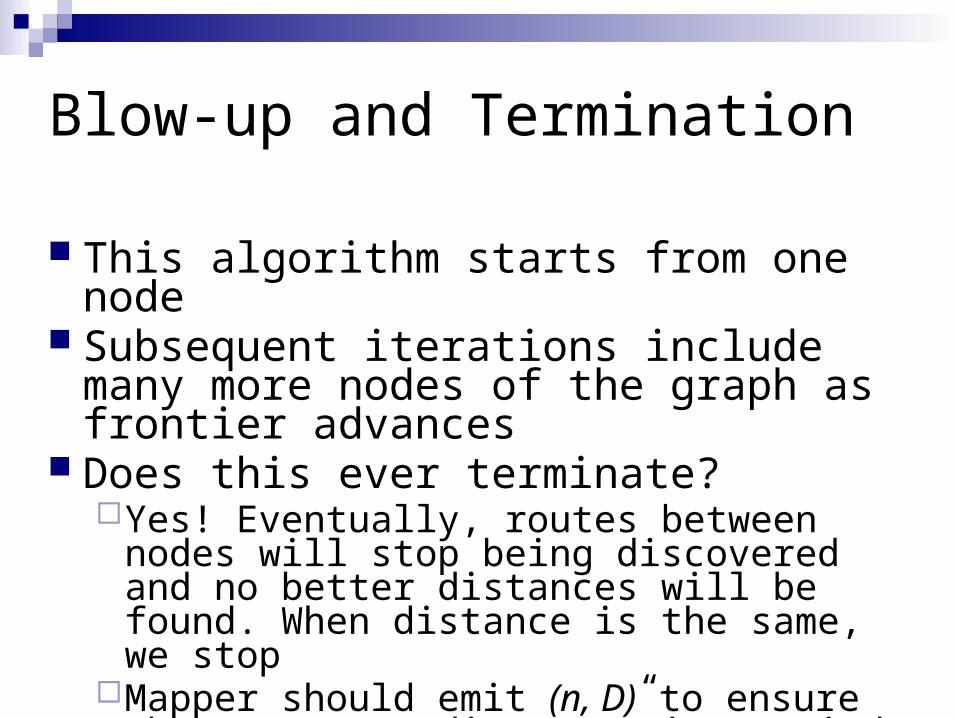
Blow-up and Termination
This algorithm starts from one node Subsequent iterations include many more
nodes of the graph as frontier advances Does this ever terminate?
Yes! Eventually, routes between nodes will stop being discovered and no better distances will be found. When distance is the same, we stop
Mapper should emit (n, D) to ensure that “current distance” is carried into the reducer
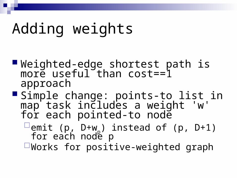
Adding weights
Weighted-edge shortest path is more useful than cost==1 approach
Simple change: points-to list in map task includes a weight 'w' for each pointed-to nodeemit (p, D+w
p) instead of (p, D+1) for each
node pWorks for positive-weighted graph
Comparison to Dijkstra
Dijkstra's algorithm is more efficient because at any step it only pursues edges from the minimum-cost path inside the frontier
MapReduce version explores all paths in parallel; not as efficient overall, but the architecture is more scalable
Equivalent to Dijkstra for weight=1 case

PageRank: Random Walks Over The Web
If a user starts at a random web page and surfs by clicking links and randomly entering new URLs, what is the probability that s/he will arrive at a given page?
The PageRank of a page captures this notionMore “popular” or “worthwhile” pages get a
higher rank
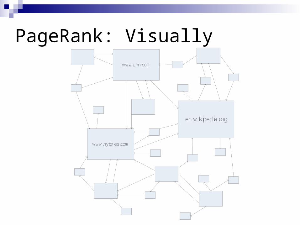
PageRank: Visuallywww.cnn.com
en.wikipedia.org
www.nytimes.com
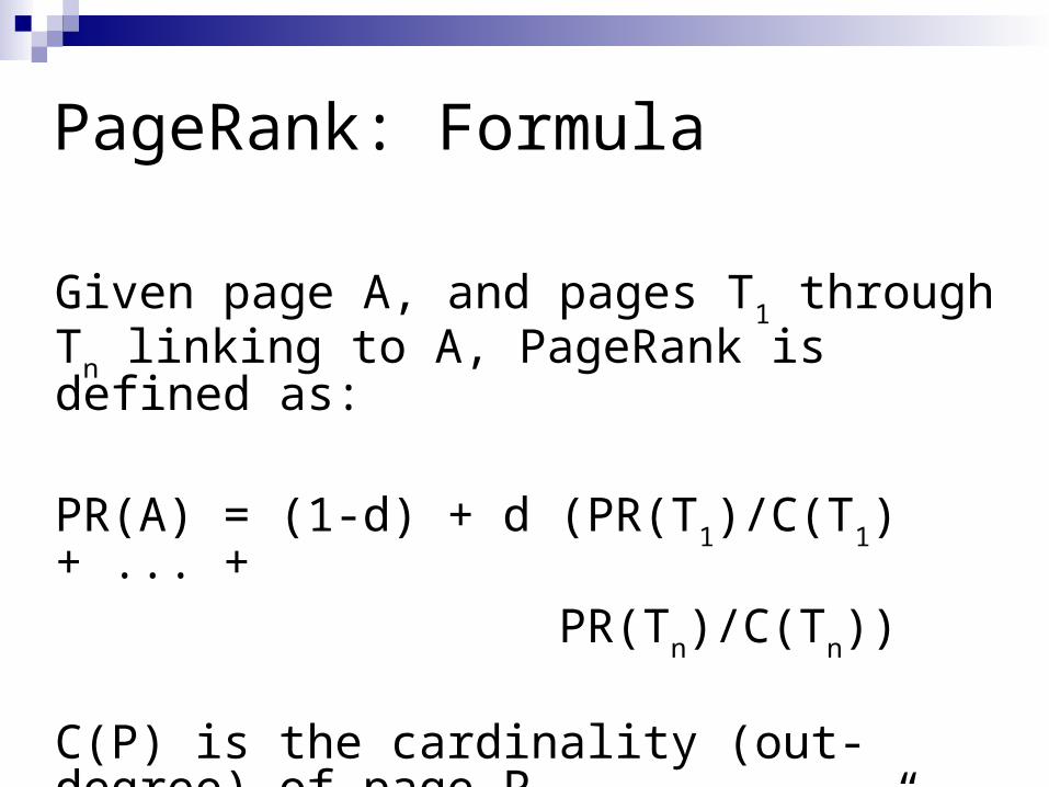
PageRank: Formula
Given page A, and pages T1 through T
n
linking to A, PageRank is defined as:
PR(A) = (1-d) + d (PR(T1)/C(T
1) + ... +
PR(Tn)/C(T
n))
C(P) is the cardinality (out-degree) of page Pd is the damping (“random URL”) factor
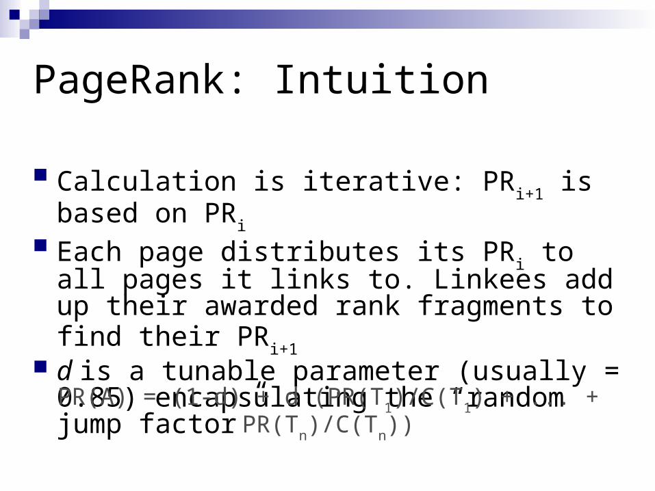
PageRank: Intuition
Calculation is iterative: PRi+1
is based on PRi
Each page distributes its PRi to all pages it
links to. Linkees add up their awarded rank fragments to find their PR
i+1 d is a tunable parameter (usually = 0.85)
encapsulating the “random jump factor”
PR(A) = (1-d) + d (PR(T1)/C(T
1) + ... + PR(T
n)/C(T
n))
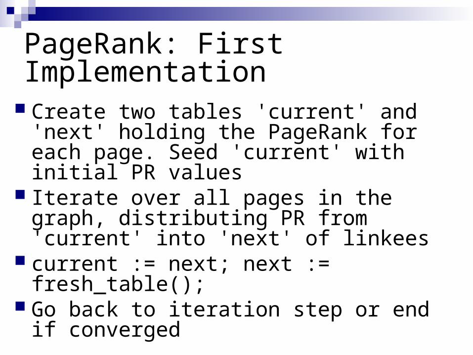
PageRank: First Implementation
Create two tables 'current' and 'next' holding the PageRank for each page. Seed 'current' with initial PR values
Iterate over all pages in the graph, distributing PR from 'current' into 'next' of linkees
current := next; next := fresh_table(); Go back to iteration step or end if converged
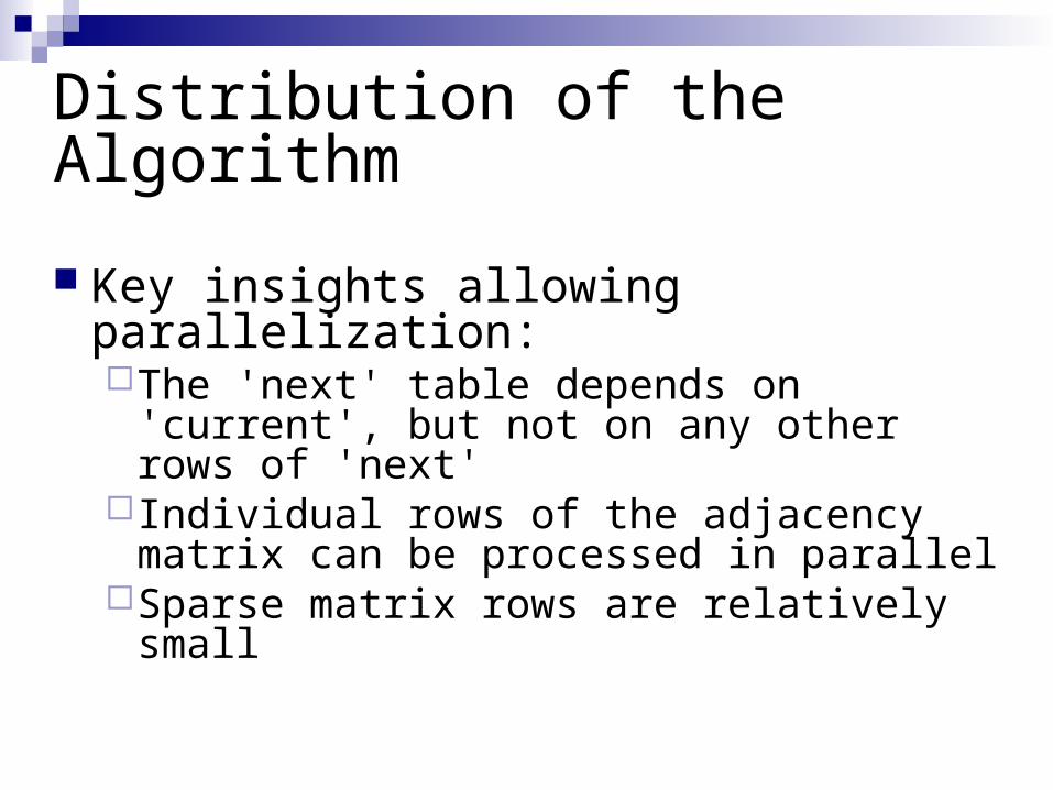
Distribution of the Algorithm
Key insights allowing parallelization:The 'next' table depends on 'current', but not on
any other rows of 'next'Individual rows of the adjacency matrix can be
processed in parallelSparse matrix rows are relatively small
Distribution of the Algorithm
Consequences of insights:We can map each row of 'current' to a list of
PageRank “fragments” to assign to linkeesThese fragments can be reduced into a single
PageRank value for a page by summingGraph representation can be even more
compact; since each element is simply 0 or 1, only transmit column numbers where it's 1
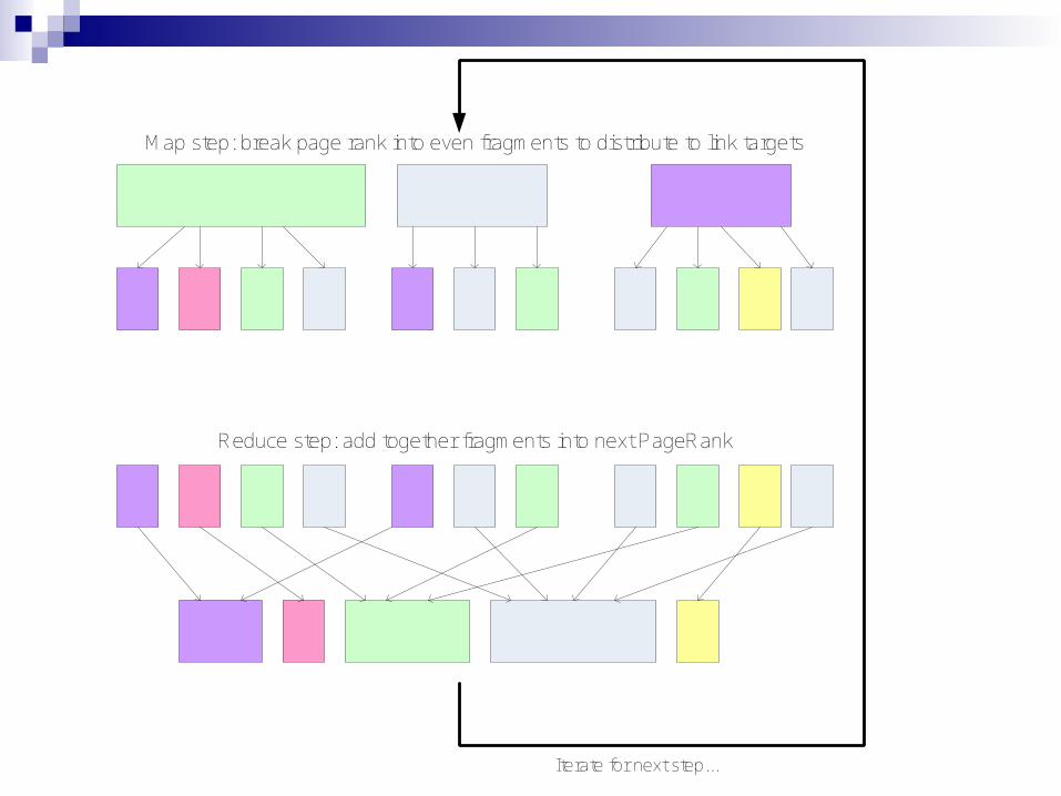
Map step: break page rank into even fragments to distribute to link targets
Reduce step: add together fragments into next PageRank
Iterate for next step...
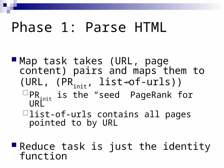
Phase 1: Parse HTML
Map task takes (URL, page content) pairs and maps them to (URL, (PR
init, list-of-urls))
PRinit
is the “seed” PageRank for URLlist-of-urls contains all pages pointed to by URL
Reduce task is just the identity function
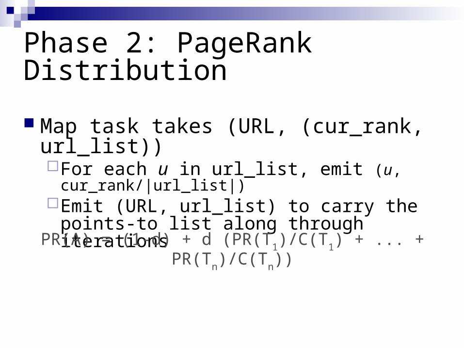
Phase 2: PageRank Distribution
Map task takes (URL, (cur_rank, url_list))For each u in url_list, emit (u, cur_rank/|url_list|)Emit (URL, url_list) to carry the points-to list
along through iterations
PR(A) = (1-d) + d (PR(T1)/C(T
1) + ... + PR(T
n)/C(T
n))
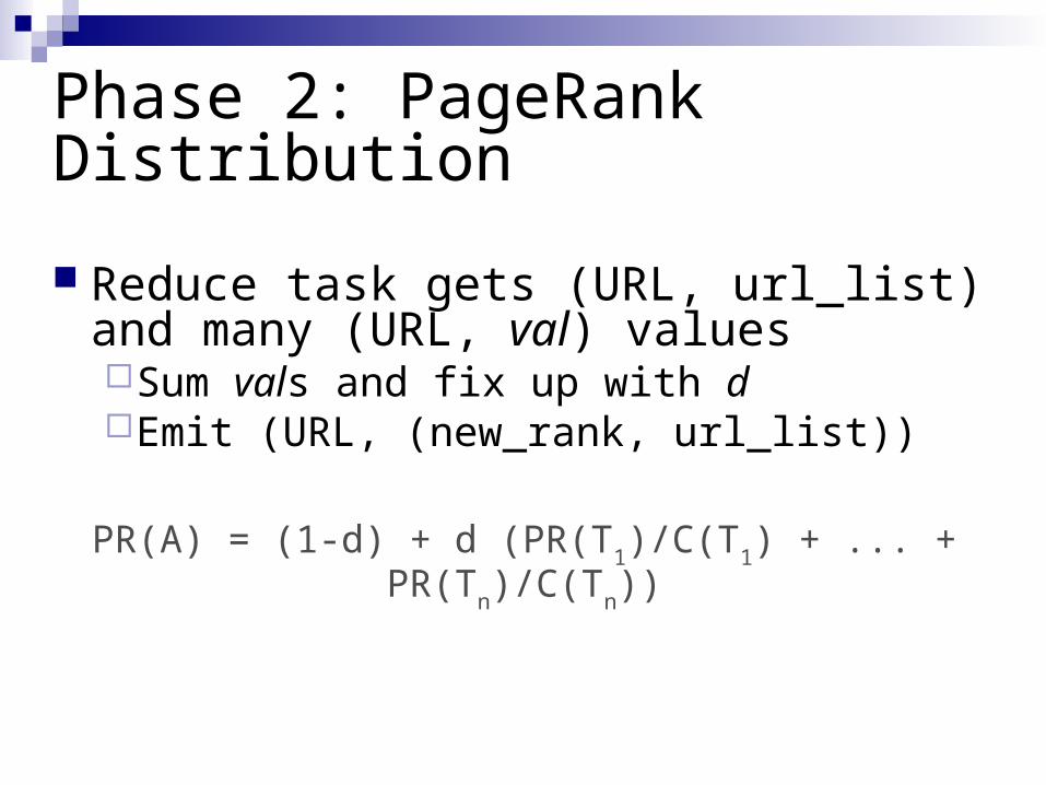
Phase 2: PageRank Distribution
Reduce task gets (URL, url_list) and many (URL, val) valuesSum vals and fix up with dEmit (URL, (new_rank, url_list))
PR(A) = (1-d) + d (PR(T1)/C(T
1) + ... + PR(T
n)/C(T
n))
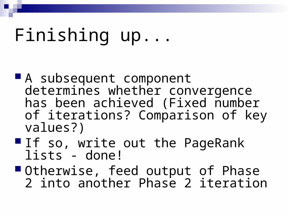
Finishing up...
A subsequent component determines whether convergence has been achieved (Fixed number of iterations? Comparison of key values?)
If so, write out the PageRank lists - done! Otherwise, feed output of Phase 2 into
another Phase 2 iteration
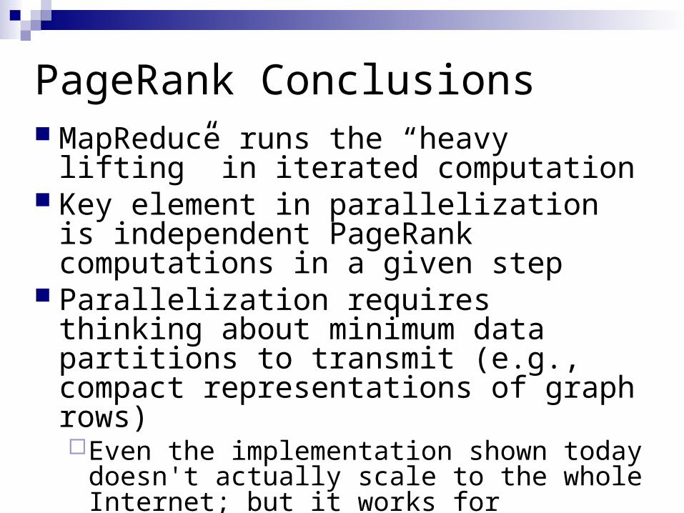
PageRank Conclusions MapReduce runs the “heavy lifting” in
iterated computation Key element in parallelization is
independent PageRank computations in a given step
Parallelization requires thinking about minimum data partitions to transmit (e.g., compact representations of graph rows)Even the implementation shown today doesn't
actually scale to the whole Internet; but it works for intermediate-sized graphs


