On real root representations of quivers
Marcel Wiedemann
Submitted in accordance with the requirements for the degree of Doctor of Philosophy
The University of Leeds
Department of Pure Mathematics
July 2008
The candidate confirms that the work submitted is his own and that appropriate credit has been given
where reference has been made to the work of others. This copy has been supplied on the understanding
that it is copyright material and that no quotation from the thesis may be published without proper
acknowledgement.
i
“GOTT GEBE MIR DIE GELASSENHEIT, DINGE HINZUNEHMEN, DIE ICH NICHT ANDERN
KANN; DEN MUT, DINGE ZU ANDERN, DIE ICH ANDERN KANN; UND DIE WEISHEIT, DAS
EINE VOM ANDEREN ZU UNTERSCHEIDEN.”
REINHOLD NIEBUHR
ii
AcknowledgementsFirst and foremost I wish to express my sincere thanks to my supervisor, Professor William W.
Crawley-Boevey. His encouragement and guidance has been of utmost importance to me during
the years of my PhD studies. I owe him everything in mathematics and I am very grateful for the
insights into the beauty of mathematics he has given me.
I would like to thank Professor Claus M. Ringel for his interest in my work and for helpful
discussions and advice.
I would also like to thank Ulrike Baumann who has listened to me for all those years and has
helped me to make the right decisions.
Finally, I am indebted to the University of Leeds for their financial support in the form of a
University Research Scholarship.
iii
AbstractLet Q be a quiver and let α be a positive real root of the associated root system. A theorem of
Kac states that there exits a unique indecomposable representation (up to isomorphism) of Q of
dimension vector α, called a real root representation.
We study real root representations and focus on the following question.
How can one “construct” real root representations and what are their “properties”?
We introduce the notion of maximal rank type for representations of quivers, which requires certain
collections of maps involved in the representation to be of maximal rank, and we show that real
root representations have the maximal rank type property.
Using the maximal rank type property and the universal extension functors introduced by Ringel
we construct all real root representations of the quiver
Q(f, g, h): 1λ1 //...λf// 2
µ1
��...µg ""
3
νh
WW ...ν1bb ,
with f, g, h ≥ 1. This shows in particular that real root representations of Q(f, g, h) are tree
representations. Moreover, formulae given by Ringel can be applied to compute the dimension of
the endomorphism ring of a given real root representation.
We ask whether this construction process involving universal extension functors generalises to
all quivers and discuss examples of representations which cannot be constructed using universal
extension functors.
iv
Contents
Quotation . . . . . . . . . . . . . . . . . . . . . . . . . . . . . . . . . . . . . . . . . i
Acknowledgements . . . . . . . . . . . . . . . . . . . . . . . . . . . . . . . . . . . . ii
Abstract . . . . . . . . . . . . . . . . . . . . . . . . . . . . . . . . . . . . . . . . . . iii
Contents . . . . . . . . . . . . . . . . . . . . . . . . . . . . . . . . . . . . . . . . . . iv
1 Introduction and outline of thesis 1
2 Background 12
2.1 Quivers, path algebras and roots . . . . . . . . . . . . . . . . . . . . . . . . . . 12
2.2 Representations of quivers and Kac’s Theorem . . . . . . . . . . . . . . . . . . 14
2.2.1 Tree representations . . . . . . . . . . . . . . . . . . . . . . . . . . . . 20
2.3 Deformed preprojective algebras and reflection functors . . . . . . . . . . . . . . 22
2.3.1 Reflection functors for representations of Πλ(Q) . . . . . . . . . . . . . 23
2.3.2 Real root representations of Q via representations of Πλ(Q) . . . . . . . 24
3 Universal extension functors 27
3.1 Construction and properties of universal extension functors . . . . . . . . . . . . 28
3.2 Real root representations of Q′′(g, h) and a generalisation . . . . . . . . . . . . . 38
CONTENTS v
4 Representations of maximal rank type and applications 41
4.1 Representations of maximal rank type . . . . . . . . . . . . . . . . . . . . . . . 41
4.2 Real root representations are of maximal rank type . . . . . . . . . . . . . . . . 43
4.3 Relation to homomorphism and extension spaces . . . . . . . . . . . . . . . . . 47
4.4 Application: representations of the quiver Q(f, g, h) . . . . . . . . . . . . . . . 52
4.4.1 The Weyl group of Q = Q(f, g, h) . . . . . . . . . . . . . . . . . . . . 54
4.4.2 Application of the maximal rank type property . . . . . . . . . . . . . . 55
4.4.3 Construction of real root representations for Q = Q(f, g, h) . . . . . . . 58
4.4.4 Further observations and comments . . . . . . . . . . . . . . . . . . . . 61
5 Two examples answering Question (††) negatively 63
5.1 Example one . . . . . . . . . . . . . . . . . . . . . . . . . . . . . . . . . . . . 65
5.2 Example two . . . . . . . . . . . . . . . . . . . . . . . . . . . . . . . . . . . . 73
6 Conclusion 79
Appendix 81
A More quivers 82
A.1 The quiver Q1 . . . . . . . . . . . . . . . . . . . . . . . . . . . . . . . . . . . . 84
A.2 The quiver Q2 . . . . . . . . . . . . . . . . . . . . . . . . . . . . . . . . . . . . 85
A.3 The six-subspace quiver . . . . . . . . . . . . . . . . . . . . . . . . . . . . . . . 88
A.4 The quiver Q4 . . . . . . . . . . . . . . . . . . . . . . . . . . . . . . . . . . . . 94
CONTENTS vi
B Research papers 98
B.1 M. Wiedemann, Representations of maximal rank type and an application to
representations of a quiver with three vertices, Bull. London Math. Soc. 40
(2008), 479-492 . . . . . . . . . . . . . . . . . . . . . . . . . . . . . . . . . . . 98
B.2 M. Wiedemann, A remark on the constructibility of real root representations using
universal extension functors, Preprint, arXiv:0802.2803 [math.RT] . . . . . . . . 100
Bibliography 102
1
Chapter 1
Introduction and outline of thesis
Algebras are objects of fundamental importance in mathematics as well as in physics. A
particularly nice example of an algebra is given by the path algebra of a quiver which is simply a
directed graph. Here is an example of a quiver
•
��@@@@@@@
• // • // • .
•
??~~~~~~~
Over the last few decades quivers have played an important role in many areas of mathematics,
including representation theory of finite dimensional algebras, the theory of Hall algebras and
quantum groups, to name but a few.
One is particularly interested in representations of an algebra; that is, the ways in which a given
algebra operates on a vector space. One of the reasons why quivers are very fruitful objects in
mathematics is because many mathematical problems, especially many problems in linear algebra,
can be reformulated in terms of representations of quivers.
In Chapter 2 we discuss quivers, representations of quivers and related results.
Chapter 1. Introduction and outline of thesis 2
One of the first milestones in the the representation theory of quivers was the work by Gabriel [11]
which classified quivers of finite representation type; that is, quivers with only finitely many non-
isomorphic indecomposable representations. Gabriel showed that a connected quiver is of finite
representation type if and only if the underlying graph is included in the following list, where the
subscript n denotes the number of vertices.
An, n ≥ 0 : • • . . . • •
•
Dn, n ≥ 4 : • • . . . •
��������
========
•
•
E6 : • • • • •
•
E7 : • • • • • •
•
E8 : • • • • • • •
The above diagrams are called Dynkin diagrams; they appear in many different areas of
mathematics, for instance the classification of finite dimensional simple Lie algebras. In [3]
Bernstein, Gelfand and Ponomarev constructed the indecomposable representations of finite
representation type quivers using certain reflection functors. The reflection functors of Bernstein,
Gelfand and Ponomarev were one of the first tools invented to study representations of quivers.
Gabriel showed that the indecomposable representations are in bijection with the positive roots
Chapter 1. Introduction and outline of thesis 3
of the corresponding finite dimensional simple Lie algebra. This bijection is provided by a
combinatorial gadget, namely root systems which are relevant to quivers as well as Lie algebras.
In the early 1980’s Kac [13] generalised Gabriel’s work to all quivers, showing that for an arbitrary
quiver the indecomposable representations correspond to the positive roots of the associated root
system. To a quiver one can also associate a Lie algebra, namely the Kac-Moody algebra. In this
way one obtains a bijection between the indecomposable representations and the positive roots of
the Kac-Moody algebra, which generalises Gabriels results. The root system of a quiver consists
of two types of roots: real roots (which can be obtained by reflections from simple roots) and
imaginary roots (which can be obtained by reflections from roots in the fundamental region). Kac
showed that for each positive real root there exists a unique indecomposable representation of
the corresponding dimension vector and for each positive imaginary root there exists a family
(depending on the size of the ground field) of non-isomorphic indecomposable representations
of the corresponding dimension vector. We call the unique indecomposable representation
corresponding to a positive real root α a real root representation and denote it by Xα.
Representations of quivers can be decomposed into indecomposable representations by the Krull-
Remak-Schmidt Theorem. Hence, in order to understand the representation theory of a given
quiver, one only needs to understand the indecomposable representations. In this thesis we focus
on certain indecomposable representations for quivers: the real root representations. We will be
concerned with the following question.
Question (†). How can one “construct” real root representations and what are their
“properties” ?
The above question is, of course, formulated rather vaguely but does nevertheless address the
central problem of this thesis. However, the terms “construct” and “properties” need to be
discussed further. What do we mean by “construct”?
So far it is not known how to construct real root representations representations in general. We
explain below certain special situations in which construction processes are known.
Chapter 1. Introduction and outline of thesis 4
We mentioned earlier that Bernstein, Gelfand and Ponomarev constructed the indecomposable
representations of finite representation type quivers (which are all real root representations) using
certain reflection functors. Hence, there are tools which give an answer to Question (†) for finite
representation type quivers.
Over an algebraically closed field of characteristic zero, Crawley-Boevey [7] gave a method
to construct real root representations of a given arbitrary quiver using deformed preprojective
algebras, discussed in Section 2.3. He showed that real root representations arise as simple
representations of deformed preprojective algebras and gave functors to construct these simple
representations. This answers part one of Question (†) over algebraically closed fields of
characteristic zero. We note that characteristic zero is essential for this construction. Moreover,
constructing real root representations in this way does not give many insights into their properties.
A different approach to the problem of constructing real root representations was given by Ringel
[18] for the following class of quivers
Q′′(g, h) : 2
µ1
��
...µg ��
3
νh
TT
...ν1YY ,
with g, h ≥ 1. Ringel showed that all real root representations of this class of quivers can be
constructed using universal extension functors, introduced in [18]. A detailed exposition of these
functors is given in Chapter 3; here we just give a brief description. Let Q be a quiver and let
k be a field. Let S be a real Schur representation of Q, that is a real root representation with
trivial endomorphism ring, then by [18, Section 1, Proposition 2] there exists an equivalence σS
(called universal extension functor) defined on certain full subcategories of the category of finite
dimensional representations of Q, namely
σS : M−S−S →MSS/S,
where M−S−S denotes the finite dimensional representations X of Q with no homomorphisms
between X and S in either way, and MSS denotes the finite dimensional representations X of
Chapter 1. Introduction and outline of thesis 5
Q with no extensions between X and S in either way and moreover, such that no direct summand
of X is generated or cogenerated by S. Moreover, MSS/S denotes the quotient category of MS
S
modulo the maps factoring through direct sums of copies of S. On a given representation X in
M−S−S the functor σS operates as follows: it extends X by copies of S at the top and at the bottom
until no non-trivial further extension is possible. Moreover, we have for X ∈M−S−S
dimσS(X) = dimX − (dimX,dimS) · dimS, and
dim EndkQ σS(X) = dim EndkQX + 〈dimX,dimS〉 · 〈dimS, dimX〉,
where dimM denotes the dimension vector of a given representation M (defined in Section
2.2), 〈−,−〉 denotes the Ringel form and (−,−) its symmetrisation (defined in Section 2.1), and
EndkQM denotes the endomorphism ring of a given representation M (defined in Section 2.2).
The description of the functor σS already shows one of the main difficulties when applying it; if
we want to apply σS to a given representation X we have to make sure that the representation X
is in the subcategory M−S−S , that is we have no homomorphisms between X and S in either way.
In [18, Section 2] Ringel constructed real root representations of Q′′ = Q′′(g, h) as follows. Let α
be a positive real root forQ′′. Write α = sin · . . . ·si1(ej) with ik, j ∈ {2, 3} and nminimal, where
si denotes the simple reflection at vertex i ∈ {2, 3} (defined in Section 2.1) and ej (j ∈ {2, 3})
denotes the simple root at vertex j (defined in Section 2.1). Then we have
Xα = σS(in) · . . . · σS(i1)(S(j)),
where S(i) (i = 2, 3) denotes the simple representation at vertex i (defined in Section 2.2). This
result and a generalisation are discussed Section 3.2.
The above construction of the real root representation Xα does not just give a way to obtain
the representation Xα, but also gives insights into the properties of Xα based on the following
fact. Namely, the functor σS allows one to keep track of certain properties of representations.
For instance, when the functor σS is applied to an indecomposable tree representation (for
definition see Section 2.2.1) the resulting representation will also be a tree representation by
Chapter 1. Introduction and outline of thesis 6
Theorem 3.1.8. Or, if we apply the functor σS to a representation of known endomorphism
ring dimension, we can easily compute the dimension of the endomorphism ring of the
resulting representation by Formula 3.1. This leads us to the second part of Question (†):
‘ ... what are their “properties” ?’. What would we like to know about real root representations?
Here are just two questions we might ask. What is the structure of the endomorphism ring, or
simpler, what is the dimension of the endomorphism ring of a given real root representation? Is a
given real root representation a tree representation?
A partial answer to the second question follows from a result of Ringel [19, Theorem].
Ringel showed that exceptional representations are tree representations, and hence real Schur
representations are tree representations. However, in general it is still open whether real root
representations are tree representations.
These questions can now be answered for an arbitrary real root representation of the quiver
Q′′(g, h), since the simple representation S(j) is trivially a tree representation (and this property
is preserved by the functors σS(ik)) and has one-dimensional endomorphism ring (and hence we
can compute the dimension of the endomorphism ring after applying the functors σS(ik)).
The heart of this thesis is the following observation which suggests a generalisation of the
above construction process for real root representations of the quiver Q′′(g, h) to other classes of
quivers. Numerical experiments with real root representations, using Crawley-Boevey’s method
to construct real root representations over algebraically closed fields of characteristic zero, show
that for certain classes of quivers we have the following behavior. Let α be a positive non-Schur
real root (a real Schur root is a positive real root such that Xα is a real Schur representation), then
there exists a real Schur root β and a positive real root γ such that
Xγ ∈M−Xβ−Xβ , and σXβ (Xγ) = Xα.
Chapter 1. Introduction and outline of thesis 7
Moreover, it follows from the theory of universal extension functors (described in Chapter 3) that
is this case we have
α = −(β, γ) · β + γ, with (β, γ) ≤ 0, and hence γ < α, and
dim EndkQXα = dim EndkQXγ + 〈β, γ〉 · 〈β, γ〉.
An indication of the numerical data supporting this claim and a description of the algorithms used
to obtain this data is given in Appendix A.
Now, if γ is not a real Schur root, we can continue this process with γ in place of α, and reduce
further in the way described above. We can do this until we arrive at a real Schur representation;
in this way we obtain for a given positive real root α a sequence βn, . . . , β1 (n ≥ 2) of real Schur
roots such that
Xα = σXβn · . . . · σXβ2 (Xβ1),
and hence we can answer the questions about Xα we are interested in (namely the question of
the dimension of its endomorphism ring, and whether it is a tree representation) once we have
answered these questions for the real Schur representation Xβ1 . But for real Schur representations
the answers to these questions are known: the dimension of the endomorphism ring is one and real
Schur representations are tree representations by Ringel’s result [19, Theorem].
In this way we have not only found a way to construct the representation Xα over an arbitrary
field but also gained an insight into certain properties of it. Concrete examples of this construction
process can be found in Appendix A.
In this thesis we approach Question (†) by focusing on the question whether the construction
process described above works for arbitrary quivers. We ask the following question.
Question (††). Let Q be a quiver and let k be a field. Let α be a positive non-Schur real root.
Does there exist a sequence βn, . . . , β1 (n ≥ 2) of real Schur roots such that
Xα = σXβn · . . . · σXβ2 (Xβ1)?
Chapter 1. Introduction and outline of thesis 8
Note, for a real Schur root β we can take the trivial sequence β, and hence we are basically
asking the question of whether all real root representations can be constructed from real Schur
representations using universal extension functors; the real Schur representations are considered
the “bricks” of this construction process. Our motivation for the above question is based on
numerical experiments with real root representations, as indicated in Appendix A. It was, however,
brought to our attention that a positive answer to Question (††) had also been conjectured by
Ringel.
In order to investigate this question further we have to develop tools to decide whether the functor
σS can be applied to a given representation, that is we have to be able to determine whether a
given representation is in the subcategory M−S−S . In Chapter 4 we discuss the maximal rank type
property, as introduced in [26]; this property can help to decide this question. The maximal rank
type property requires certain collections of maps involved in the representation to be of maximal
rank. The collections of maps considered are the following: for a given vertex and a collection
of incoming vertices we can form the sum of these maps and equally for a collection of outgoing
vertices. A representation is said to be of maximal rank type if all these maps have maximal rank.
The maximal rank type property of real root representations is one of the authors main results.
Theorem ([26, Theorem A]). LetQ be a quiver and let α be a positive real root forQ. The unique
indecomposable representation of dimension vector α is of maximal rank type.
In Section 4.3 we discuss implications of the maximal rank type property of real root
representations. One implication is that the dimension of homomorphism spaces and extension
spaces between real root representations and simple representations are determined by the Ringel
form, and hence are completely combinatorial. In particular, this gives a way to decide whether a
real root representation is in the subcategory M−S−S , for S a simple representation associated to a
vertex of a given quiver Q.
In Section 4.4 we use the maximal rank type property to construct real root representations of the
quiver
Chapter 1. Introduction and outline of thesis 9
Q(f, g, h): 1λ1 //...λf// 2
µ1
��
...µg ��
3
νh
TT
...ν1YY ,
with f, g, h ≥ 1.
The quiver Q(1, 1, 1) was considered by Jensen and Su in [12], where all real root representations
were constructed explicitly. Moreover, it was shown that all real root representations are tree
representations, and formulae to compute the dimensions of the endomorphism rings were given.
In [20] Ringel extended their results to the quiver Q(1, g, h) (g, h ≥ 1) using universal extension
functors.
The main result of Section 4.4 is the following.
Theorem ([26, Theorem B]). Let α be a positive real root for the quiver Q(f, g, h). The unique
indecomposable representation of dimension vector α can be constructed by using universal
extension functors starting from simple representations and real Schur representations of the
quiver Q′(f) (f ≥ 1), where Q′(f) denotes the following subquiver of Q(f, g, h)
Q′(f): 1λ1 //...λf// 2 .
The sequence of real Schur roots βn, . . . , β1 can be obtained in a purely combinatorial way: one
only needs to write the real root α in a certain admissible form (described in Section 4.4). We
consider an example. Let α be the following real root for Q(f, g, h) with f ≥ 2.
α = s1 s2 s1 s3 s2 s1 s2 s1 s2 s3 s1 s2 (e3).
The real root α is already written in admissible form. The real Schur roots βn, . . . , β1 can
be obtained as follows. Each occurrence of s3 gives the real Schur root e3. The symmetric
expressions not involving s3 give a real Schur root of the subquiver Q′(f). It can be obtained by
taking the left half of the expression and replacing the reflection in the middle by the corresponding
Chapter 1. Introduction and outline of thesis 10
simple root. The real Schur root corresponding to the rightmost non-symmetric expression not
involving s3, here s1 s2, is the one corresponding to the symmetrisation of it. This process gives
the following real Schur roots for the above example
α = s1 s2 s1
���O�O�O�O�O�O�O�O
s3
�� �O�O�O�O�O�O�O�O�O
s2 s1 s2 s1 s2
���O�O�O�O�O�O�O�O
s3
�� �O�O�O�O�O�O�O�O�O
s1 s2
���O�O�O
(e3),
s1 s2 s1
�� �O�O�O
s1(e2) e3 s2 s1(e2) e3 s1(e2)
and hence
β6 = s1(e2), β5 = e3, β4 = s2 s1(e2), β3 = e3, β2 = s1(e2), β1 = e3.
The real root representation Xα of dimension vector α can be constructed as follows
Xα = σXβ6 σXβ5 σXβ4 σXβ3 σXβ2 (Xβ1).
The class Q(f, g, h), (f, g, h ≥ 1) of quivers provides another example for which Question (††)
can be answered positively. Moreover, it provides further motivation to study Question (††) in
general.
In Chapter 5 we discuss Question (††) in full generality and show that the answer is negative in
general. The main result of Chapter 5 is the following example of a real root representation which
cannot be constructed in this way.
Consider the quiver
Q : 1 a//
b
%%2 c
//
d
<<3 e// 4 ,
and the real root representation Xα with dimension vector α = (1, 8, 6, 4). Our main result is the
following.
Chapter 1. Introduction and outline of thesis 11
Theorem. The real root representation Xα is not Schur and there does not exist a sequence of
real Schur roots βn, . . . , β1 such that
Xα = σXβn · . . . · σXβ2 (Xβ1).
Moreover, we discuss further questions arising from this representation.
The main results of this thesis form the content of the paper [26] and the preprint [25], which is
available on the Mathematics ArXiv website. Both research articles are included in Appendix B.
12
Chapter 2
Background
In this chapter we discuss background material and related results. We start with an overview of
quivers and representations of quivers. A more detailed exposition of these topics can be found
in [1, Chapter II], [2, Chapter III] and [5, 6]. The references given usually refer to the article in
which the result first appeared. For standard results we just give a textbook reference.
In the last section of this chapter we discuss Crawley-Boevey’s method to construct real root
representations in characteristic zero.
2.1 Quivers, path algebras and roots
Definition 2.1.1. A quiver Q = (Q0, Q1, h, t) is a finite directed graph with vertex set Q0, arrow
set Q1 and two maps h, t : Q1 → Q0 which assign to each arrow a ∈ Q1 its head h(a) ∈ Q0 and
its tail t(a) ∈ Q0. In particular, we write a : t(a)→ h(a) for a ∈ Q1.
A quiver Q = (Q0, Q1, h, t) is usually just denoted by Q. The opposite quiver Qop =
(Q0, Q1, hop = t, top = h) of a quiver Q is obtained by reversing all arrows. A subquiver of
a quiver Q = (Q0, Q1, h, t) is a quiver Q′ = (Q′0, Q′1, h′, t′) with Q′0 ⊂ Q0, Q′1 ⊂ Q1, h′ = h|Q′1
Chapter 2. Background 13
and t′ = t|Q′1 . A subquiver Q′ of Q is called full if
Q′1 = {a ∈ Q1 : h(a) ∈ Q′0, t(a) ∈ Q′0}.
A loop is an arrow a ∈ Q1 with h(a) = t(a). A path p of Q is a sequence p = a1 . . . an of
arrows ai ∈ Q1 such that t(ai) = h(ai+1) for i = 1, . . . , n − 1. We define h(p) = h(a1) and
t(p) = t(an). Moreover, for each vertex i ∈ Q0 we have a trivial path εi with h(εi) = t(εi) = i.
The path algebra kQ of a quiver Q = (Q0, Q1, h, t) is defined as follows. It has as k-basis all
the paths (including the trivial paths) of Q. The multiplication of two paths p1 and p2 is given by
the concatenation p1 p2 if h(p2) = t(p1) and zero otherwise. This defines an associative k-algebra
with∑
i∈Q0εi being the identity element.
The Ringel form on ZQ0 is the bilinear form defined by
〈α, β〉 :=∑
i∈Q0
α[i]β[i]−∑
a∈Q1
α[t(a)]β[h(a)], α, β ∈ ZQ0 .
Let (α, β) := 〈α, β〉+ 〈β, α〉 be its symmetrisation.
The Ringel form is represented in the natural basis of ZQ0 by the Euler matrix E = (bij)i,j∈Q0 ,
defined by
bij = δi,j − card {a ∈ Q1 : t(a) = i, h(a) = j},
where di,j is the Kronecker delta symbol.
The root lattice of a quiver Q is given by ZQ0 together with the quadratic form q(α) = 12(α, α).
We write ei ∈ ZQ0 for the coordinate vector at vertex i and by α[i], i ∈ Q0, we denote the i-
th coordinate of α ∈ ZQ0 . The support of α ∈ ZQ0 is the full subquiver of Q with vertex set
{i ∈ Q0 : α[i] 6= 0}. An element α ∈ ZQ0 is said to be sincere if α[i] > 0 for all i ∈ Q0.
Let i ∈ Q0 be a loop-free vertex of Q; then there is a simple reflection si : ZQ0 → ZQ0 defined
by
si(α) := α− (α, ei)ei.
Chapter 2. Background 14
The Weyl group, denoted by W , is the subgroup of GL(ZQ0) generated by the si.
A simple root is a vector ei for i ∈ Q0. We denote by Π the set of simple roots ei with i loop-free.
By ∆+re(Q) := {α ∈ W (Π) : α ∈ ZQ0 , α > 0} we denote the set of (positive) real roots for Q.
For a positive real root α we define the following reflection sα : ZQ0 → ZQ0
sα(β) := β − (β, α) · α.
The fundamental region is defined as follows
M := {α ∈ NQ0 : α 6= 0, α has connected support and (α, ei) ≤ 0 for all i ∈ Q0}.
By ∆+im(Q) :=
⋃w∈W w(M) we denote the set of (positive) imaginary roots for Q.
Moreover, we define by ∆+(Q) := ∆+re(Q) ∪ ∆+
im(Q) the set of positive roots. We have the
following fundamental lemma.
Lemma 2.1.2 ([13, Lemma 2.1]). Let Q be a quiver without loops. For α ∈ ∆+(Q) one has
(i) α ∈ ∆+re(Q) if and only if 〈α, α〉 = 1,
(ii) α ∈ ∆+im(Q) if and only if 〈α, α〉 ≤ 0.
2.2 Representations of quivers and Kac’s Theorem
In this section we fix a quiver Q and a field k.
Definition 2.2.1. A k-linear representation or, simply, a representation X = (Xi, Xa)i∈Q0,a∈Q1
of Q is defined by the following data:
(i) a finite dimensional k-vector space Xi for each i ∈ Q0 and
(ii) a k-linear map Xa : Xt(a) → Xh(a) for each a ∈ Q1.
Chapter 2. Background 15
Let i, j ∈ Q0 and let ni,j be the number of arrows from i to j. The above definition of a
representation X of Q is equivalent to the following definition.
Definition 2.2.2. A k-linear representation or, simply, a representation X = (Xi, Xi,j)i,j∈Q0 of
Q is defined by the following data:
(i)’ a finite dimensional k-vector space Xi for each i ∈ Q0 and
(ii)’ a k-linear map Xi,j : Xi ⊗k kni,j → Xj for all i, j ∈ Q0.
Here the maps for the individual arrows from i to j are encoded in the vector space kni,j . One
can pass from the second definition to first by choosing a basis of kni,j . Moreover, we have the
following natural vector-space isomorphisms
Homk(Xi ⊗ kni,j , Xj) ∼= Homk(Xi,Homk(kni,j , Xj)) ∼= Homk(Xi, Xj ⊗ kni,j ).
In this way, given a map Xi,j : Xi ⊗k kni,j → Xj one obtains a map X ′i,j : Xi → Xj ⊗ kni,j .
We shall usually work with Definition 2.2.1; only in Chapter 4 we work with Definition 2.2.2.
Example 2.2.3 (Simple representation). We denote by S(i) the representation
S(i)j =
k, i = j,
0, i 6= j,
∀ j ∈ Q0, S(i)a = 0 ∀ a ∈ Q1.
Example 2.2.4 (Dual representation). Let X be a representation of Q. We denote by X∗ the
representation of Qop, defined as follows:
(X∗)i = (Xi)∗ ∀ i ∈ Q0, (X∗)a = (Xa)∗ ∀ a ∈ Q1.
The dimension vector dimX of a representation X is defined by
dimX = (dimXi)i∈Q0 ∈ ZQ0 .
Let X = (Xi, Xa)i∈Q0,a∈Q1 and Y = (Yi, Ya)i∈Q0,a∈Q1 be two representations of Q. A
homomorphism ψ : X → Y is defined by a family ψ = (ψi)i∈Q0 of k-linear maps ψi : Xi →
Yi (i ∈ Q0) such that for each arrow a ∈ Q1 the square
Chapter 2. Background 16
Xt(a)Xa //
ψt(a)��
Xh(a)
ψh(a)
��Yt(a)
Ya// Yh(a)
commutes.
The direct sum X ⊕ Y of two representations X and Y is defined by
(X ⊕ Y )i = Xi ⊕ Yi, ∀ i ∈ Q0,
(X ⊕ Y )a =
Xa 0
0 Ya
, ∀ a ∈ Q1.
A representation Z is called decomposable if Z is isomorphic to X ⊕ Y for non-zero
representations X and Y .
We denote by repkQ the category of finite dimensional representations of Q.
There is an equivalence between the category repkQ and the category of finite dimensional left
kQ-modules, given by the following construction. A representation X = (Xi, Xa)i∈Q0,a∈Q1
defines a kQ-module M as follows: M := ⊕i∈Q0Xi with εi acting as the projection onto Xi and
with an arrow a : i → j acting as the following composition M εi−→ XiXa−→ Xj
incl.−→ M . This
defines a finite dimension left kQ-module. On the other hand, a finite dimensional kQ-module M
defines a representation of Q as follows: Xi := εi ·M for each i ∈ Q0 and Xa : εt(a) ·M →
εh(a) ·M,m 7→ a ·m for each a ∈ Q1. This construction is functorial.
Theorem 2.2.5 ([2, Chapter III, Theorem 1.5]). The category of finite dimensional left kQ-
modules is equivalent to the category repkQ.
In particular it follows that repkQ is an abelian k-category.
One may also want to consider representations of quivers with relations. Namely, let I ⊂ kQ be
an ideal with generators ui ∈ kQ (i = 1, . . . , n) such that ui ∈ εkikQεli for ki, li ∈ Q0. Let
X = (Xi, Xa)i∈Q0,a∈Q1 be representation of Q. A path p = a1 . . . an in Q defines a linear map
Chapter 2. Background 17
Xp = Xa1 ◦ . . . ◦ Xan : Xt(p) → Xh(p). In this way every generator ui ∈ I defines a linear
map Xui : Xli → Xki . We denote by repk(Q, I) the full subcategory of repkQ consisting of
representations X = (Xi, Xa)i∈Q0,a∈Q1 of Q such that Xui = 0 for all i = 1, . . . , n.
In the same way as above, the category of finite dimensional left kQ/I-modules can be identified
with the category repk(Q, I)
Theorem 2.2.6 ([2, Chapter III, Proposition 1.7]). The category of finite dimensional left kQ/I-
modules is equivalent to the category repk(Q, I).
We only consider quivers with relations in Section 2.3, where we discuss deformed preprojective
algebras. Our main focus is on the category repkQ.
One of the key properties of the category repkQ is the Krull-Remak-Schmidt property.
Theorem 2.2.7 ([16, Part two, Chapter X, Section 7, Theorem 7.5]). Let X be a representation of
Q. Then
X =n⊕
i=1
Xi,
with Xi indecomposable for i = 1, . . . , n. This decomposition is unique up to isomorphism and
reordering of the summands.
We will not discuss homological properties of the category repkQ; we refer the reader to [1,
Section VII.1] and [2, Chapter III] for a discussion of relevant homological properties of repkQ.
An overview of basic notions of homological algebra can be found in [1, Appendix A.4]. We only
mention that the category repkQ is hereditary, which implies that Ext2kQ(X,Y ) = 0 for any two
representations X and Y of Q, see [2, Chapter III, Proposition 1.4 and following comments] or
use the standard resolution [5, §1, The standard resolution].
The construction of the extension space Ext1kQ(X,Y ) of two representations X and Y of a quiver
Q, as discussed in [19, Section 2] and [17, Section 2.1], can be done in the following elementary
way.
Chapter 2. Background 18
Let X and Y be representations of Q and let
C0(X,Y ) :=⊕
i∈Q0
Homk(Xi, Yi),
C1(X,Y ) :=⊕
a∈Q1
Homk(Xt(a), Yh(a)).
We define the map
δXY : C0(X,Y ) → C1(X,Y )
(φi)i 7→ (φjXa − Yaφi)a:i→j .
The importance of δXY is given by the following lemma.
Lemma 2.2.8 ([17, Section 2.1, Lemma]). We have ker δXY = HomkQ(X,Y ) and coker δXY =
Ext1kQ(X,Y ).
It follows from the above lemma that for two representations X and Y we have the following
useful formula
dim HomkQ(X,Y )− dim Ext1kQ(X,Y ) = 〈dimX,dimY 〉.
The heredity of the category repkQ implies the following two facts.
Let 0 → X → Y → Z → 0 be a short exact sequence of representations
of Q, for a representation M of Q we have the following long exact sequences
0 // HomkQ(M,X) // HomkQ(M,Y ) // HomkQ(M,Z) EDJKONHI
00aaaaa Ext1kQ(M,X) // Ext1kQ(M,Y ) // Ext1kQ(M,Z) // 0,
0 // HomkQ(Z,M) // HomkQ(Y,M) // HomkQ(X,M) MLJKONHI
11bbbbb Ext1kQ(Z,M) // Ext1kQ(Y,M) // Ext1kQ(X,M) // 0.
Chapter 2. Background 19
When studying representations of Q our main interest lies in indecomposable representations,
as suggested by Theorem 2.2.7. As already mentioned in the introduction, the indecomposable
representations of Q correspond to the positive roots ∆+(Q), see [13, 14, 15]. We have the
following remarkable theorem, generally known as Kac’s Theorem.
Theorem 2.2.9 (Kac [13, Theorem 1 and 2], Schofield [22, Theorem 9]). Let k be a field, let Q
be a quiver without loops and let α ∈ NQ0 .
(i) For α /∈ ∆+(Q) all representations of Q of dimension vector α are decomposable.
(ii) For α ∈ ∆+re(Q) there exists one and only one (up to isomorphism) indecomposable
representation of dimension vector α.
For finite fields and algebraically closed fields the theorem is due to Kac [13, Theorem 1 and 2].
As pointed out in the introduction of [22], Kac’s method of proof showed that the above theorem
holds for fields of characteristic p. The proof for fields of characteristic zero is due to Schofield
([22], Theorem 9).
Remark 2.2.10. In Section 2.3 we discuss an alternative proof of part (ii) of this result over an
algebraically closed field of characteristic zero, given by Crawley-Boevey.
We are now able to precisely define the objects discussed in the introduction: real root
representations. The work presented in the later chapters focuses on these objects, motivated
by Question (†) and Question (††).
Definition 2.2.11 (Real root representation). Let Q be a quiver and let α be a positive real root.
The unique indecomposable representation (up to isomorphism) of dimension vector α is called a
real root representation and denoted by Xα.
We finish this section with some further definitions. A Schur representation is a representation X
with EndkQ(X) = k. By a real Schur representation we mean a real root representation which
is also a Schur representation. A positive real root α is called a real Schur root if Xα is a real
Chapter 2. Background 20
Schur representation. Note that Ext1kQ(Xα, Xα) = 0 for α a real Schur root. An indecomposable
representation X is called exceptional provided Ext1kQ(X,X) = 0.
By X = Y for two given representations X and Y we mean that X and Y are isomorphic.
2.2.1 Tree representations
In the introduction the question of properties of real root representations was raised. One of the
questions was whether real root representations are tree representations? We use this section to
discuss this notion and relevant results. Our elaborations are mainly based on the article [19] by
Ringel.
Let Q = (Q0, Q1, h, t) be a quiver and let k be a field. Moreover, let X ∈ repkQ be a
representation of Q with dimX = d. We denote by Bi a fixed basis of the vector space
Xi (i ∈ Q0) and set B = ∪i∈Q0Bi. The set B is called a basis ofX . We fix a basis B ofX . For a
given arrow a : i→ j we can write Xa as a d[j]× d[i]-matrix Xa,B with rows indexed by Bj and
with columns indexed by Bi. We denote by Xa,B(x, x′) the corresponding matrix entry, where
x ∈ Bi, x′ ∈ Bj ; the entries Xa,B(x, x′) are defined by Xa(x) =
∑x′∈Bj
Xa,B(x, x′)x′. The
coefficient quiver Γ(X,B) ofX with respect to B is defined as follows: the vertex set of Γ(X,B)
is the set B of basis elements ofX; there is an arrow (a, x, x′) between two basis elements x ∈ Bi
and x′ ∈ Bj provided Xa,B(x, x′) 6= 0 for a : i→ j.
Let B and B′ be two bases of X . B and B′ are said to proportional if for every b ∈ B there
exists a non-zero λ(b) ∈ k such that λ(b) · b ∈ B′. In this case the coefficient quivers Γ(X,B)
and Γ(X,B′) may be identified.
Definition 2.2.12 (Tree module, see [19]). We call an indecomposable representation X of Q a
tree representation provided there exists a basis B of X such that the coefficient quiver Γ(X,B)
is a tree.
Example 2.2.13. Consider the quiver A3 and the following representation X together with the
corresponding coefficient quiver Γ(X,B), where B is given by the canonical basis of k2 and k.
Chapter 2. Background 21
k •
X : k2
[1 1]??��������
[0 1] ��>>>>>>>>, Γ(X,B) : •
55kkkkkkkkkkkkkkkkkkkk •
%%LLLLLLLLLLLLL
99rrrrrrrrrrrrr
k •
Note, the coefficient quiver Γ(X,B) is connected. For the following matrix presentation of X the
coefficient quiver is not connected.
k •
X : k2
[1 0]??��������
[0 1] ��>>>>>>>>, Γ(X,B) : •
55kkkkkkkkkkkkkkkkkkkk •
%%LLLLLLLLLLLLL
k •
We see that the coefficient quiver Γ(X,B) may be connected even if X is decomposable.
The coefficient quiver Γ(X,B) has the following properties.
Lemma 2.2.14 ([19, Section 2, Property 1]). If X is indecomposable and B is a basis of X then
Γ(X,B) is connected. If X is decomposable then there exists a basis B of X such that Γ(X,B)
is not connected.
Lemma 2.2.15 ([19, Section 2, Property 2]). Let B be a basis of X such that Γ(X,B) is a
tree. Then there is a basis B′ of X which is proportional to B such that all non-zero coefficients
Xa,B′(x, x′) are equal to 1.
The following remarkable theorem is due to Ringel.
Theorem 2.2.16 ([19, Theorem]). Let k be a field and let Q be a quiver. Any exceptional
representation of Q over k is a tree representation.
In particular, real Schur representations are tree representations. The importance of this fact
was already mentioned in the introduction. Since the property of being a tree representation
Chapter 2. Background 22
is preserved under universal extension functors (see Chapter 3), we see that if a real root
representation can be constructed from a real Schur representation using universal functors, this
property will be preserved.
2.3 Deformed preprojective algebras and reflection functors
We mentioned in the introduction that Crawley-Boevey constructed real root representations for
an arbitrary quiver over algebraically closed fields of characteristic zero. In this section we give a
detailed description of Crawley-Boevey’s results. We use the results of this section in Chapter 5
and in Appendix A.
We start by describing deformed preprojective algebras, a generalization of preprojective algebras,
and discuss reflection functors for these algebras. In the second part we relate real root
representations to simple representations of deformed preprojective algebras, which can be
constructed using the reflection functors.
Let Q = (Q0, Q1, h, t) be a quiver and let k be a field. The double quiver Q is obtained by
adjoining a reverse arrow a∗ : j → i for each arrow a : i → j in Q. For λ ∈ kQ0 the deformed
preprojective algebra Πλ(Q), introduced by Crawley-Boevey and Holland in [8], is the algebra
defined by
Πλ(Q) = kQ/
∑
a∈Q1
[a, a∗]−∑
i∈Q0
λ[i]εi
where [a, a∗] = aa∗ − a∗a. If Q′ is obtained from Q by reversing the arrow a, then there is an
isomorphism Πλ(Q) → Πλ(Q′) which sends a to a∗ and a∗ to −a. Hence, it is clear that Πλ(Q)
does not depend on the orientation ofQ. A representationX of Πλ(Q) is given by a representation
X of Q, say, with vector space Xi at vertex i ∈ Q0 and linear map Xa : Xt(a) → Xh(a) for each
arrow a ∈ Q, which satisfies
∑
a∈Qh(a)=i
XaXa∗ −∑
a∈Qt(a)=i
Xa∗Xa = λ[i] idXi ,
Chapter 2. Background 23
for each vertex i ∈ Q0.
2.3.1 Reflection functors for representations of Πλ(Q)
Let i ∈ Q0 be a loop-free vertex. The dual reflection ri : kQ0 → kQ0 to si is defined by
ri(λ)[j] := λ[j]− (ei, ej)λ[i],
and it satisfies ri(λ) · α = λ · si(α) for all α ∈ ZQ0 and all λ ∈ kQ0 . Let λ ∈ kQ0 . We recall a
theorem from [8].
Theorem 2.3.1 ([8, Theorem 5.1]). If i ∈ Q0 is a loop-free vertex, λ[i] 6= 0, then there is an
equivalence
Ei : Πλ(Q)-modules→ Πri(λ)(Q)-modules
which acts as the simple reflection si on dimension vectors.
We use the rest of this section to recall the construction of this functor. Let X be a representation
of Πλ(Q) and let i be a loop-free vertex ofQ with λ[i] 6= 0. We define T (i) = {a ∈ Q : t(a) = i}
and X⊕ =⊕
a∈T (i)Xh(a). For a ∈ T (i) we define the following canonical projection and
inclusion maps
πa : X⊕ → Xh(a),
µa : Xh(a) → X⊕.
Moreover, we define µ : Xi → X⊕ and π : X⊕ → Xi by
µ =∑
a∈T (i)
µaXa,
π =1λ[i]
∑
a∈T (i)
−ε(a)Xa∗πa
where ε is defined as follows: ε(a) = 1 for a ∈ Q1, and ε(a) = −1 for
a ∈ Q1 − Q1; in addition to this we are using the following convention: for a ∈ Q1 we define
Chapter 2. Background 24
(a∗)∗ := a. The relations for Πλ(Q) ensure that πµ = 1Xi , and hence µπ is an idempotent
endomorphism of X⊕.
We define a representation X ′ of Πri(λ)(Q) as follows:
X ′j = Xj , for j 6= i,
X ′i = kerπ = im (1− µπ),
together with the following maps: X ′a = Xa for a ∈ Q1 with t(a) 6= i 6= h(a), and
X ′a = −ε(a)λ[i](1− µπ)µa∗ : X ′t(a) → X ′i, if h(a) = i,
X ′a = πa|X′i : X ′i → X ′h(a), if t(a) = i.
Lemma 2.3.2. X ′ is a representation of Πri(λ)(Q).
Proof. See proof of [8, Theorem 5.1].
The reflection functor Ei : Πλ(Q) → Πri(λ)(Q) sends a representation X to Ei(X) := X ′ and
operates on homomorphisms in the natural way.
2.3.2 Real root representations of Q via representations of Πλ(Q)
In this section we discuss two of Crawley-Boevey’s results from [7] which relate real root
representations of Q to simple representations of Πλ(Q). This gives an algorithm to construct
real root representations over algebraically closed fields of characteristic zero.
The first result we need concerns the question of lifting representations of Q to representations of
Πλ(Q).
Theorem 2.3.3 ([7, Theorem 3.3]). Let k be an algebraically closed field. If λ ∈ kQ0 then a
representation of Q lifts to a representation of Πλ(Q) if and only if the dimension vector β of any
direct summand satisfies λ · β = 0.
Chapter 2. Background 25
Remark 2.3.4. No assumption for the field is needed for the “=⇒” direction.
This result and the reflection functors described in Section 2.3.1 can be used to construct real root
representations of Q over an algebraically closed field of characteristic zero. We give Crawley-
Boevey’s proof, since it is very instructive.
Proposition 2.3.5 ([7, Proposition A.4]). Let k be an algebraically closed field of characteristic
zero, and let α be a real root for Q. Choose a reflection series
α = sin . . . si1(ej)
such that α(k) = sik . . . si1(ej) is not a coordinate vector for 1 ≤ k ≤ n. Let λ(0) ∈ kQ0 be the
vector with λ(0)[j] = 0 and λ(0)[i] = 1 for all i 6= j, and define λ(k) = rik(λ(k−1)) for 1 ≤ k ≤ n.
Then λ(k)[ik+1] 6= 0 for all k. Moreover, there is a unique indecomposable representation of Q of
dimension α, and it may be obtained from the simple representation of Πλ(0)(Q) of dimension ej
by applying successively the reflection functors at the vertices ik, and then restricting the resulting
representation of Πλ(n)(Q) to Q.
Proof. Since k has characteristic zero, λ(0) ·β 6= 0 for any root β which is not equal to±ej . Using
the formula ri(λ) · α = λ · si(α), it follows that λ(t) · β 6= 0 for any root β which is not equal to
±α(t). In particular, λ(t) · eit+1 6= 0 for t ≥ 0. Thus λ(k)[ik+1] 6= 0 for all k.
Using the equivalence Ei in Theorem 2.3.1, we get an equivalence between representations of
Πλ(0)(Q) of dimension vector ej , of which there is only one, and representations of Πλ(m)
(Q)
of dimension α. Thus, up to isomorphism, there is a unique representation Xα of Πλ(m)(Q),
of dimension vector α. Note that this representation is simple. The restriction of Xα to Q is
indecomposable, for if it had an indecomposable direct summand of dimension β, Theorem 2.3.3
would imply λ(m) · β = 0 (here were are using the “=⇒” direction). This is impossible since β is
a root not equal to ±α.
Finally, observe that any indecomposable representation of Q of dimension α lifts to a
representation of Πλ(m)(Q) of dimension α, because λ(m) · α = 0. Up to isomorphism there
Chapter 2. Background 26
is only one representation of Πλ(m)(Q) of dimension α, hence it follows that there is only one
indecomposable representation of Q of dimension α, up to isomorphism.
Remark 2.3.6. Characteristic zero is essential for this construction method.
Remark 2.3.7. In Section 2.2 we discussed Theorem 2.2.9, a remarkable Theorem due to Kac
and Schofield. The previous proposition gives an alternative proof of this result over algebraically
closed fields of characteristic zero.
27
Chapter 3
Universal extension functors
This chapter is devoted to a detailed discussion of the universal extension functors σS which
were introduced by Ringel in [18]. We recall all necessary definitions and results from [18]
which are needed to describe these functors. Moreover, we prove that universal extension functors
preserve indecomposable tree representations. In the last part of this section we discuss Ringel’s
construction of real root representations of the quiver
Q′′(g, h) : 2
µ1
��
...µg ��
3
νh
TT
...ν1YY ,
with g, h ≥ 1 and a generalisation of this result.
In this chapter we assume some familiarity with the concepts of categories and functors. For a
basic account of category theory, functors and related notions we refer the reader to [1, Appendix
A.1 and A.2].
Chapter 3. Universal extension functors 28
3.1 Construction and properties of universal extension functors
Let Q be a quiver and let k be a field. We fix a real Schur representation S of Q; that is, a
representation S with EndkQ S = k and Ext1kQ(S, S) = 0.
For a full subcategory C of repkQ we define by C/S the quotient category of C modulo all maps
which factor thourgh direct sums of copies of S.
In analogy to [18, Section 1], we define the following subcategories of repkQ. Let MS be the
full subcategory of all modules X with Ext1kQ(S,X) = 0 such that, in addition, X has no direct
summand which can be embedded into some direct sum of copies of S. Similarly, let MS be
the full subcategory of all modules X with Ext1kQ(X,S) = 0 such that, in addition, no direct
summand ofX is a quotient of a direct sum of copies of S. Finally, let M−S be the full subcategory
of all modules X with HomkQ(X,S) = 0, and let M−S be the full subcategory of all modules X
with HomkQ(S,X) = 0. Moreover, we consider
MSS = MS ∩MS , M−S−S = M−S ∩M−S .
For a given module X we define by X−S the intersection of the kernels of all maps X → S.
Moreover, we define X−S = X/X ′, where X ′ is the sum of the images of all maps S → X .
Remark 3.1.1. Let X,Y ∈ repkQ and let f : X → Y . For x ∈ X−S we have to have that
f(x) ∈ Y −S , and hence f(X−S) ⊂ Y −S . Thus, we obtain the following functor repkQ →
repkQ,X 7→ X−S , which operates on homomorphisms by restriction. Moreover, if f : X → Y
factors through a direct sum of copies of S then we have X−S ⊂ ker f and the restriction of f to
X−S is zero.
Dually, we obtain a functor repkQ→ repkQ,X 7→ X−S .
Let X ∈ MS . Since X does not split off a copy of S (because EndkQ S = k and X ∈ MS ,
and hence no direct summand of X embeds into a sum of copies of S) we have to have that any
f : S → X maps into X−S , and hence the natural map HomkQ(S,X−S) → HomkQ(S,X) is
Chapter 3. Universal extension functors 29
an isomorphism. Similarly, it follows for X ∈ MS that the natural map HomkQ(X−S , S) →
HomkQ(X,S) is an isomorphism.
Lemma 3.1.2 ([18, Lemma 1]). For any X ∈ repkQ, we have X−S ∈M−S .
Dual-Lemma 3.1.2. For any Y ∈ repkQ, we have Y−S ∈M−S .
Lemma 3.1.3 ([18, Lemma 2]). Let X ∈MS and let φ1, . . . , φr be a basis of the k-vector space
HomkQ(X,S). Then the sequence
0→ X−S → X(φ1,...,φr)t−→
r⊕
i=1
S → 0
is exact and the induced sequences E1, . . . , Er ∈ ExtkQ(S,X−S) form a basis of the k-vector
space Ext1kQ(S,X−S).
Dual-Lemma 3.1.3. Let Y ∈ MS and let φ′1, . . . , φ′u be a basis of the k-vector space
HomkQ(S, Y ). Then the sequence
0→u⊕
i=1
S(φ′1,...,φ
′u)−→ Y → Y−S → 0
is exact and the induced sequences E′1, . . . , E′u ∈ ExtkQ(Y−S , S) form a basis of the k-vector
space Ext1kQ(Y−S , S).
Lemma 3.1.4 ([18, Lemma 3]). Let X ∈ M−S and let E1, . . . , Es be a basis of the k-vector
space Ext1kQ(S,X). Consider the exact sequence E
E : 0→ X → Z →s⊕
i=1
S → 0
given by the elements Ej (j = 1, . . . , s). Then Z ∈MS and Z−S = X .
Dual-Lemma 3.1.4. Let Y ∈ M−S and let E′1, . . . , E′v be a basis of the k-vector space
Ext1kQ(Y, S). Consider the exact sequence E′
E′ : 0→v⊕
i=1
S → U → Y → 0
given by the elements E′j (j = 1, . . . , v). Then U ∈MS and U−S = Y .
Chapter 3. Universal extension functors 30
Proposition 3.1.5 ([18, Proposition 1]). The functor ψS : MS/S →M−S , X 7→ X−S defines an
equivalence.
It follows from Remark 3.1.1 and Lemma 3.1.2 that ψS defines indeed a functor between the
respective categories. Moreover, it is clear by Remark 3.1.1 that maps in MS which factor through
a direct sum of copies of S get sent to the zero map. Hence, in order to obtain an equivalence we
certainly have to factor out all the maps factoring through a direct sum of copies of S. This,
however, is already enough by [18, Proposition 1] and makes the functor ψS full and faithful,
meaning that it is an isomorphism on homomorphism spaces. The functor is dense, meaning that
for every Y ∈ M−S there exists a X ∈ MS such that X−S = Y , by Lemma 3.1.4. Hence, the
functor ψS is full, faithful and dense. It is a well known fact (e.g. see Theorem [1, Theorem 2.5,
Appendix A.2]) that this implies that the functor is an equivalence. We denote a quasi-inverse of
this equivalence by σS : M−S → MS/S; it operates on objects as follows (up to isomorphism).
Let X ∈ M−S and let Z ∈ MS be the representation constructed in Lemma 3.1.4, then we have
σS(X) = Z. We remark that the construction of the representation Z ∈ MS depends on the
choice of a basis of the k-vector space Ext1kQ(S,X). Different choices however, give isomorphic
representations by Lemma 3.1.4. Since we are only studying representations up to isomorphisms
this description of a quasi-inverse is sufficient for us.
We have the following dual result.
Dual-Proposition 3.1.5 ([18, Proposition 1∗]). The functor ψS
: MS/S → M−S , Y 7→ Y−S
defines an equivalence.
We denote a quasi-inverse of this equivalence by σS : M−S → MS/S; it operates on objects as
follows. Let Y ∈M−S and let U ∈MS be the representation constructed in Dual-Lemma 3.1.4,
then we have σS(Y ) = U .
Proposition 3.1.6 ([18, Proposition 2]). The functor ψS : MSS/S → M−S−S , X 7→ (X−S)−S
defines an equivalence.
Chapter 3. Universal extension functors 31
Idea of proof. The functor ψS can be constructed as follows. Firstly, we restrict the equivalence
ψS to the following equivalence
ψS : MSS/S →M−SS , X 7→ X−S .
This can be done by the following arguments. Let X ∈ MSS = MS ∩MS , by Lemma 3.1.3 we
get
0→ X−S → X →r⊕
i=1
S → 0, r = dim HomkQ(X,S),
and hence, using long exact sequences (described in Section 2.2) and the fact that
Ext1kQ(S, S) = 0, it follows that
Ext1kQ(X,S) = 0←→ Ext1kQ(X−S , S) = 0.
Moreover, we must show that (by the second part of definition MS)
X = X1 ⊕X2, X1 is a quotient of a direct sum of copies of S
←→ X−S = Y1 ⊕ Y2, Y1 is a quotient of a direct sum of copies of S.
If X = X1 ⊕X2 and⊕S
µ� X1 then we have
0→ X−S → X1 ⊕X2[ν1,ν2]−→
r⊕
i=1
S → 0,
with ν1 = 0, since X does not split off a copy of S (see Remark 3.1.1). This implies
X−S = X1 ⊕ ker ν2. If X−S = Y1 ⊕ Y2 and⊕S
µ� Y1 then we get (use long exact sequence)
Ext1kQ(S,⊕S) � Ext1kQ(S, Y1), and hence Ext1kQ(S, Y1) = 0, since Ext1kQ(S, S) = 0. Since
we have
0→ X−S → X →r⊕
i=1
S → 0, r = dim HomkQ(X,S),
this implies that X ∼= Y1 ⊕ Z with 0→ Y2 → Z →⊕ri=1 S → 0.
Secondly, we restrict the equivalence ψS
to the following equivalence
ψS
: M−SS →M−S−S , Y 7→ Y−S .
Chapter 3. Universal extension functors 32
This can be done by the following arguments. By definition, in the category M−SS there are
no homomorphisms factoring through direct sums of copies of S. Hence, we do not need
to consider a quotient category. Now, let Y ∈ MS . By Remark 3.1.1 the natural map
HomkQ(Y −S , S)→ HomkQ(Y, S) is an isomorphism, and thus
HomkQ(Y −S , S) = 0←→ Hom1kQ(Y, S) = 0.
The functor ψS is defined to be ψS ◦ ψS ; this makes sense by the above elaborations. In
the same way we could define ψS to be ψS◦ ψS (using arguments dual to the ones given
above). In the following we show that the order in which we apply ψS
and ψS does not matter
(up to isomorphism). That is, for a given representation in X ∈ MSS we need to show that
ψS◦ ψS(X) = (X−S)−S = (X−S)−S = ψS ◦ ψS(X). Let X ∈ MS
S , then we have by Lemma
3.1.3 and Dual-Lemma 3.1.3
0→ X−S → X →r⊕
i=1
S → 0, r = dim HomkQ(X,S),
0→u⊕
i=1
S → X → X−S → 0, u = dim HomkQ(S,X).
By Remark 3.1.1 the natural maps HomkQ(S,X−S) → HomkQ(S,X) and
HomkQ(X−S , S) → HomkQ(X,S) are isomorphisms. Thus, we get the following commuting
diagram.
0
��
0
��
0
��0 //
⊕ui=1 S
//
��
⊕ui=1 S
//
��
0 //
��
0
0 // X−S //
��
X //
��
⊕ri=1 S
//
��
0
0 // (X−S)−S //
��
X−S //
��
⊕ri=1 S
//
��
0
0 0 0
Chapter 3. Universal extension functors 33
The top and the middle rows are exact, and hence so is the bottom row. (This is the 3× 3 lemma,
which can be found in [24, Exercise 1.3.2]). This, however, is the exact sequence as constructed
in Lemma 3.1.3, and hence (X−S)−S = (X−S)−S .
We denote a quasi-inverse of the equivalence ψS by σS : M−S−S → MSS/S and call the functor
σS universal extension functor. The above proof shows that the functor σS operates on objects by
applying the constructions for σS and σS successively. Moreover, the order in which we apply σS
and σS does not matter, which follows from the fact that in the construction of ψS the order of ψS
and ψS
did not matter. By [18, Proposition 2] we have
dimσS(X) = sdimS(dimX), and
dimψS(X) = sdimS(dimX).
One of the main problems when applying the functor σS was already mentioned in the introduction
and becomes clear now: if we want to apply the equivalence σS to a representation X , we must
haveX ∈M−S−S . WhetherX ∈M−S−S orX /∈M−S−S is one of the main questions we are concerned
with. In Chapter 4 we discuss the maximal rank type property which may be used to decide this
question for real root representations.
In the introduction we raised two questions about properties of real root representations. What
is the dimension of the endomorphism ring of a given real root representation? Is a given
real root representation a tree representation? Since we are concerned with the question of the
constructibility of real root representations using universal extension functors, it is essential for us
to know how these properties behave under the functor σS . This is discussed in the following two
results.
Proposition 3.1.7 ([18, Proposition 3 & 3∗]). Let X ∈M−S−S . Then
dim EndkQ σS(X) = dim EndkQ(X) + 〈dimX,dimS〉 · 〈dimS, dimX〉. (3.1)
Let Y ∈MSS . Then
dim EndkQ ψS(Y ) = dim EndkQ(Y )− 〈dimY, dimS〉 · 〈dimS, dimY 〉.
Chapter 3. Universal extension functors 34
The following result shows that indecomposable tree representations are preserved under the
functors σS , σS and σS . The proof follows closely the arguments given in [19, Section 3 and
Section 6].
Theorem 3.1.8 ([26, Lemma 3.16]). Let X ∈ M−S (resp., X ∈ M−S) be an indecomposable
tree representation. Then the representation σS(X) (resp., σS(X)) is an indecomposable tree
representation. In particular, let X ∈ M−S−S be an indecomposable tree representation, then
σS(X) is an indecomposable tree representation.
Proof. We consider only the situation for the functor σS . The situation for σS is analogous. Since
σS is given by applying σS and σS successively, the second assertion follows from the first.
We recall the construction of σS(X). Let E1, . . . , Es be a basis of the k-vector space
Ext1kQ(S,X). Consider the exact sequence E given by the elements E1, . . . , Es
E : 0→ X → Z →s⊕
i=1
S → 0; (+)
then we have σS(X) = Z. First of all, we note that Z is indecomposable since
σS : M−S → MS/S defines an equivalence of categories by Proposition 3.1.5. It follows from
Theorem 2.2.16 that the representation S is a tree representation. Thus, we can choose a basis BX
ofX and a basis BS of S such that the corresponding coefficient quivers Γ(X,BX) and Γ(S,BS)
are trees. We set dX :=∑
i∈Q0dimXi (dimension of X) and dS :=
∑i∈Q0
dimSi (dimension
of S). It follows that Γ(X,BX) has dX − 1 arrows and Γ(S,BS) has dS − 1 arrows.
Let a ∈ Q1. For given 1 ≤ s ≤ dimS[t(a)] and 1 ≤ t ≤ dimX[h(a)] we denote by
MSX(a, s, t) ∈ Homk(St(a), Xh(a))
the matrix unit with entry one in the column with index s and the row with index t, and zeros
elsewhere. The set
HSX := {MSX(a, s, t) : a ∈ Q1, 1 ≤ s ≤ dimS[t(a)], 1 ≤ t ≤ dimX[h(a)]}
Chapter 3. Universal extension functors 35
is clearly a basis of C1(S,X). Hence, we can choose a subset
Φ := {MSX(ai, si, ti) : 1 ≤ i ≤ r} ⊂ HSX
such that span Φ ⊕ im δSX = C1(S,X), which implies that the residue classes
φ + im δSX (φ ∈ Φ) form a basis of Ext1kQ(S,X); these elements are responsible for obtaining
the extension (+).
We are now able describe the matrices of the representation Z with respect to the basis BX ∪⋃rd=1 BS . Let b ∈ Q1. The matrix Zb has the following form
Zb =
Xb N(b, 1) . . . N(b, r)
Sb. . .
Sb
with all other entries equal to zero and
N(b, i) =
M(ai, si, ti), if b = ai
0, otherwise,
where 0 denotes the zero matrix of the appropriate size. This explicit description allows us to
count the overall number of non-zero entries in the matrices of the representation Z with respect
to the basis BX ∪⋃rd=1 BS : this number equals the number of arrows of the coefficient quiver
Γ(Z,BX ∪⋃rd=1 BS). We easily see that there are
(dX − 1) + r(dS − 1) + |Φ| = dX + rdS − 1 =∑
i∈Q0
dimZi − 1
non-zero entries.
Now, since Z is indecomposable, the coefficient quiver Γ(Z,BX ∪⋃rd=1 BS) is connected, and
hence Γ(Z,BX ∪⋃rd=1 BS) is a tree.
Chapter 3. Universal extension functors 36
We fix the following notation.
Definition 3.1.9. Let α be a real Schur root for Q. We define
M−α−α := M−Xα−Xα , Mαα := MXα
Xα, and σα := σXα .
The following lemma shall be used frequently throughout this thesis.
Lemma 3.1.10. Let k be a field and let Q be a quiver. Let β be a real Schur root and let γ be a
real root such that Xγ ∈M−β−β . Then we have Xα = σβ(Xγ) with α = sβ(γ).
Proof. Since Xγ ∈ M−β−β the functor σβ can be applied to Xγ and we set Z = σβ(Xγ). The
representation Z is indecomposable, since the representation Xγ is indecomposable. Moreover,
we get dimZ = α by formula 3.1. By Kac’s Theorem 2.2.9, however, there exists only one
indecomposable representation (up to isomorphism) of dimension vector α. Hence, we get the
desired result Xα = Z.
We demonstrate the functor σS in an example.
Example 3.1.11. Let k be a field. Consider the quiver Q : 1 // // 2 . Clearly, S(2) ∈ M−e1−e1
since both representations have disjoint support, and hence the functor σe1 can be applied to S(2).
Moreover, we have
dim Ext1kQ(S(1), S(2)) = 2 (given by the two arrows),
dim Ext1kQ(S(2), S(1)) = 0.
Hence, we get
0→ S(2)→ σe1(S(2))→2⊕
i=1
S(1)→ 0,
where σe1(S(2)) is the real root representation with dimension vector α = (2, 1), by Lemma
3.1.10. By construction, the representation Xα has the following matrix form.
Chapter 3. Universal extension functors 37
k2
[0,1]
��[1,0]
��k
Moreover, Xα is a tree representation by the previous theorem, and we get by Formula 3.1
dim EndkQXα = dim EndkQ S(2) + 〈e2, e1〉 · 〈e1, e2〉
= 1 + 0 = 1.
We give a first example of a class of quivers for which Question (††) can be answered affirmatively.
Example 3.1.12. Let k be a field and let Q be an extended Dynkin quiver. For a discussion of the
representation theory of extended Dynkin quivers see [5] (over algebraically closed fields) and [9]
(over arbitrary fields, using the more general species approach).
Let α be a non-Schur real root. It follows thatXα is a non-homogeneous regular representation and
has the following regular composition factors (where τ denotes the Auslander-Reiten translate)
T, τT, τ2T, τ3T, . . . , τ rT, r ≥ 1
with T a regular simple representation and τ r+1T 6= T , since α is a real root. We consider
two cases. Firstly, let T 6= τ rT . Consider the real root representation Xγ with the following
composition factors
T, τT, τ2T, τ3T, . . . , τ r−1T.
Thus Xγ ∈ M−Xβ−Xβ with Xβ = τ rT (which is a regular simple), since the representation Xγ is
uniserial (see [9]), that is it has a unique composition series, and T 6= τ rT and τ r−1T 6= τ rT
(because T 6= τT , since we are in a tube of length greater than one). Namely, a map φ : Xγ → Xβ
would imply that Xγ/ kerφ = Xβ , and hence T = τ rT (by uniseriality) which is impossible. On
the other hand, a map φ : Xβ → Xγ would imply (by uniseriality) that τ r−1T = τ rT which is
impossible. Hence Xα = σXβ (Xγ) by Lemma 3.1.10.
Chapter 3. Universal extension functors 38
Secondly, let T = τ rT . Consider the real root representation Xγ with the following composition
factors
τT, τ2T, τ3T, . . . , τ r−1T.
Thus Xγ ∈ M−Xβ−Xβ with Xβ = T (which is a regular simple), since the representation Xγ is
uniserial and T 6= τT (as above) and T 6= τ r−1T (because τ rT = T = τ r−1T implies that
T = τT ); together with a similar reasoning as above. Hence, Xα = σXβ (Xγ), by Lemma 3.1.10.
3.2 Real root representations of Q′′(g, h) and a generalisation
We now consider the following quiver
Q′′(g, h) : 2
µ1
��
...µg ��
3
νh
TT
...ν1YY ,
with g, h ≥ 1. As mentioned in the introduction, Question (††) can be answered affirmatively for
Q′′(g, h), (g, h) ≥ 1. This is due to the following key lemma.
Lemma 3.2.1 ([18, Lemma 4]). Let k be a field and let Q be a quiver. Let S, T be representations
of Q, where T is simple.
(i) If Ext1kQ(S, T ) 6= 0, then MS ⊂M−T .
(ii) If Ext1kQ(T, S) 6= 0, then MS ⊂M−T .
We have the following immediate corollary for the quiver Q′′(g, h), (g, h ≥ 1).
Corollary 3.2.2. We have
Me2e2 ⊂ M−e3−e3 ,
Me3e3 ⊂ M−e2−e2 .
Chapter 3. Universal extension functors 39
The above corollary and Lemma 3.1.8 together with the trivial fact that
S(2) ∈M−e3−e3 and S(3) ∈M−e2−e2 ,
imply the following theorem, already mentioned in the introduction.
Theorem 3.2.3 ([18, Section 2]). Let k be a field and let α be a positive
real root for Q′′(g, h), (g, h ≥ 1). Write α = sin · . . . · si1(ej)
with ik, j ∈ {2, 3} and n minimal. Then we have
Xα = σein · . . . · σei1 (S(j)),
and hence the representationXα is a tree representation and formula (3.1) can be used to compute
dim EndkQXα.
The above result can be generalized to quivers with the following property (#) for all
i, j ∈ Q0: if there exists a ∈ Q1 with a : i→ j then there exists a′ ∈ Q1 with a′ : j → i.
Example 3.2.4. Here is an example of a quiver Q with the above property (#).
Q : 1((
AA2((
hh 3hh��
Theorem 3.2.5. Let k be a field. Let Q be a quiver with the property (#)
and let α be a positive real root for Q. Write α = sin · . . . · si1(ej)
with ik, j ∈ Q0 and n minimal. Then we have
Xα = σein · . . . · σei1 (S(j)),
and hence the representationXα is a tree representation and formula (3.1) can be used to compute
dim EndkQXα.
Proof. We prove the assertion by induction on n. The induction base n = 1 is trivial, since
S(j) ∈M−ei1−ei1 , and hence σei1 can be applied. Thus Xα = σei1 (S(j)) by Lemma 3.1.10.
Chapter 3. Universal extension functors 40
Let n > 1 and consider α = sin · . . . · si1(ej) with n minimal. We set i0 = j and
α′ = sin−1 · . . . · si1(ej). Assume that ip 6= in for 0 ≤ p ≤ n − 2. In this case we clearly
have Xα′ ∈ M−ein−ein and, thus Xα = σein (Xα′) by Lemma 3.1.10 and the assertion follows by
induction.
Now, assume there exists 0 ≤ p ≤ n − 2 such that in = ip and choose p maximal. Since n
is minimal and from the assumption on the quiver it follows that there exists p < q < n and
a, a′ ∈ Q1 such that a : iq → in and a′ : in → iq. (If not, then sin and siq commute for
p < q < n, and hence n is not minimal.) In particular, using Lemma 3.2.1, we get
Meiqeiq ⊂M
−ein−ein .
By induction we have σeiq · . . . · σei1 (S(j)) ∈ Meiqeiq ∩ M
−eiq+1
−eiq+1, and hence
σeiq · . . . · σei1 (S(j)) ∈ M−ein−ein ∩ M
−eiq+1
−eiq+1. Now, let Y ∈ M
−ein−ein ∩ M
−eit−eit with it 6= in.
We can apply σeit to Y and we get (by construction of the universal extension functor)
0 → Y → σS(it)(Y )→r⊕
i=1
S(it)→ 0, r = dim Ext1kQ(S(it), X)
0 →u⊕
i=1
S(it)→ σeit (Y )→ σS(it)(Y )→ 0, u = dim Ext1kQ(σS(it)(Y ), S(it)).
Using long exact sequences (as described in Section 2.2) and the fact that S(in) � S(it) (since
in 6= it), we see that σeit (Y ) ∈M−ein−ein .
Now, by induction we know that σeiq · . . . · σei1 (S(j)) ∈ M−ein−ein , and from the choice of p it
follows that ir 6= in for all p < r < n. Hence, the above elaborations imply that
Xα′ = σein−1· . . . · σei1 (S(j)) ∈M
−ein−ein ,
and thus Xα = σein (Xα′) by Lemma 3.1.10, and the assertion follows.
The representation Xα is a tree representation by Lemma 3.1.8.
41
Chapter 4
Representations of maximal rank type
and applications
In the last chapter it became clear that if we want to work with the equivalence σS , we need to be
able to decide for a given representation X whether X ∈M−S−S or X /∈M−S−S . In this chapter we
discuss the maximal rank type property which may be used to answer this question.
In order to obtain a more general result than in [26, Theorem A] we shall work with Definition
2.2.2 of a representation in this chapter.
4.1 Representations of maximal rank type
Let Q = (Q0, Q1, h, t) be a quiver and let k be a field. For i ∈ Q0 we define the sets
HQ(i) := {a ∈ Q1 : h(a) = i} and TQ(i) := {a ∈ Q1 : t(a) = i}.
Definition 4.1.1 (Maximal rank type). A representationX ofQ is said to be of maximal rank type,
provided it satisfies the following conditions.
(i) For every vertex i ∈ Q0 and for every family of vector subspaces Uj,i ⊂ knj,i (j ∈ Q0) the
Chapter 4. Representations of maximal rank type and applications 42
map
⊕
j∈Q0
Xj ⊗k Uj,iXj,i−→ Xi
is of maximal rank.
(ii) For every vertex i ∈ Q0 and for every family of vector subspaces Ui,j ⊂ kni,j (j ∈ Q0) the
map
Xi
X′i,j−→⊕
j∈Q0
Xj ⊗ Ui,j
is of maximal rank.
Remark 4.1.2. In the paper [26] the author introduced the following definition.
Definiton (Maximal rank type, [26, Definition]). A representation X of Q is said to be of
maximal rank type, provided it satisfies the following conditions.
(i) For every vertex i ∈ Q0 and for every subset A ⊆ HQ(i) the map
⊕
a∈AXt(a)
(Xa)a−→ Xi
is of maximal rank.
(ii) For every vertex i ∈ Q0 and for every subset B ⊆ TQ(i) the map
Xi(Xb)b−→
⊕
b∈BXh(b)
is of maximal rank.
We remark that Definition 4.1.1 is stronger than the above definition, since we are not only
allowing arrows but also independent linear combinations of arrows.
Clearly not every representation of Q is of maximal rank type. The following example shows that
even indecomposable representations of Q might not be of maximal rank type:
k1 //
0// k .
Chapter 4. Representations of maximal rank type and applications 43
4.2 Real root representations are of maximal rank type
In this section we show that real root representations are of maximal rank type. The main idea of
the proof is to insert an extra vertex and to attach to it the image of the considered map. Analysing
this modified representation yields the desired result. The technicalities for inserting an extra
vertex are discussed in the first part of this section followed by the proof of the main result.
Let Q = (Q0, Q1, h, t) be a quiver without loops and let k be a field. Moreover, let i ∈ Q0 be
a vertex of Q and let X be a representation of Q. For a given family U = (Uj,i)j∈Q0 of vector
subspaces Uj,i ⊂ knj,i (j ∈ Q0) we define the quiverQiU and the representationXiU (of the quiver
QiU ) as follows
(QiU )0 := Q0 ∪ {z}, (QiU )1 := (Q1 −HQ(i))
∪ {γpUj,i : j ∈ Q1, 1 ≤ p ≤ dimUj,i}
∪ {γpj,i : j ∈ Q1, 1 ≤ p ≤ nj,i − dimUj,i}
∪ {δ}
with
t(γpUj,i) := j, h(γpUj,i) := z ∀ j ∈ Q0, 1 ≤ p ≤ dimU(j,i),
t(γpj,i) := j, h(γpj,i) := i ∀ j ∈ Q0, 1 ≤ p ≤ nj,i − dimU(j,i),
t(δ) := z, h(δ) := i,
(heads and tails for all arrows in Q1 −HQ(i) remain unchanged) and
(XiU )j := Xj ∀ j ∈ Q0, (Xi
U )z := im
⊕
j∈Q0
Xj ⊗k Uj,iXj,i−→ Xi
⊂ Xi,
with maps
(XiU )f,g := Xf,g ∀ f, g ∈ Q0 − {i, j},
(XiU )z,i := inclusion,
(XiU )j,i := restriction of Xj,i to direct complement of Uj,i ∀ j ∈ Q0,
(XiU )j,z := Xj,z ∀ j ∈ Q0,
Chapter 4. Representations of maximal rank type and applications 44
where Xj,z : Xj ⊗k Ui,j → (XiU )z is the unique linear map with (Xi
U )z,i ◦ Xj,z = Xj,i; and all
other maps zero.
The construction above gives a functor F iU : repkQ→ repkQiU , defined as follows:
F iU : Ob(repkQ) → Ob(repkQiU )
X 7→ XiU ,
with the natural definition for morphisms. Moreover, there is a natural functor
iUG : repkQiU → repkQ, defined by
iUG : Ob(repkQ
iU ) → Ob(repkQ)
X 7→ iUG(X),
with
(iUG(X))j := Xj ∀ j ∈ Q0,
and maps
(iUG(X))f,g := Xf,g ∀ f, g ∈ Q0 − {i, j},
(iUG(X))j,i :=
Xj,i, if dimUj,i = 0
Xz,i ◦Xj,z, otherwise, ∀ j ∈ Q0
and all other maps zero, together with the natural definition for morphisms. The functor iUG is
left-adjoint to the functor F iU , and iUG ◦ F iU is naturally isomorphic to the identity functor on
repkQ.
We get the following useful lemma.
Lemma 4.2.1. Let i ∈ Q0 and let X be a representation of Q. If X is indecomposable, then so is
F iU (X) = XiU for every family U = (Uj,i)j∈Q0 .
Chapter 4. Representations of maximal rank type and applications 45
Proof. Assume that XiU = F iU (X) ∼= V ⊕W , then X ∼= i
UG ◦ F iU (X) ∼= iUG(V )⊕ i
UG(W ). By
assumption X is indecomposable, so w.l.o.g. we can assume that iAG(V ) = 0. Hence,
0 = HomkQ(iUG(V ), X) = HomkQiU(V, F iUX) = HomkQiU
(V, V ⊕W ),
which is only possible in case V = 0. This proves the assertion.
We are now able to prove the maximal rank type property of real root representations.
Theorem 4.2.2. Let Q be a quiver and let α be a positive real root for Q. The unique
indecomposable representation of dimension vector α is of maximal rank type.
Proof. Let α be a real root for Q, and let X = Xα be the unique indecomposable representation
of Q of dimension vector α. Moreover, let i ∈ Q0 and let U = (Uj,i)j∈Q0 be a family of vector
subspaces Uj,i ⊂ knj,i (j ∈ Q0). We have to show that the map
⊕
j∈Q0
Xj ⊗k Uj,iXj,i−→ Xi
has maximal rank. This is equivalent to showing that
dim(XiU )z = min
∑
j∈Q0
α[j] dimUj,i, α[i]
,
The representation XiU of QiU is indecomposable by Lemma 4.2.1. It follows from Theorem 2.2.9
that dimXiU ∈ ∆+(QiU ). Hence, by Lemma 2.1.2, 〈α, α〉 ≤ 1, where α := dimXi
U . We have
〈α, α〉 = 〈α, α〉︸ ︷︷ ︸=1
+∑
j∈Q0
α[j](dimUj,i)α[i] + α[z]2 − α[z]α[i]−∑
j∈Q0
α[j](dimUj,i)α[z]
= 1 +
α[z]−
∑
j∈Q0
α[j] dimUj,i
· (α[z]− α[i]) ≤ 1,
and henceα[z]−
∑
j∈Q0
α[j] dimUj,i
· (α[z]− α[i]) ≤ 0.
Chapter 4. Representations of maximal rank type and applications 46
However, we clearly have α[z] ≤ min{∑
j∈Q0α[j] dimUj,i, α[i]
}, by definition of Xi
U . This
implies thatα[z]−
∑
j∈Q0
α[j] dimUj,i
· (α[z]− α[i]) = 0;
that is, α[z] = min{∑
j∈Q0α[j] dimUj,i, α[i]
}, and hence
dim(XiU )z = min
∑
j∈Q0
α[j] dimUj,i, α[i]
.
This shows that the map⊕
j∈Q0Xj ⊗k Uj,i
Xj,i−→ Xi has maximal rank.
Dually, for a given family U = (Uj,i)j∈Q0 to show that the map
Xi
X′i,j−→⊕
j∈Q0
Xj ⊗ Ui,j
has maximal rank is equivalent to showing that the map
⊕
j∈Q0
(X ⊗ Ui,j)∗(X′i,j)
∗
−→ X∗i
has maximal rank, where ∗ denotes the vector space dual. This follows from what is proved above
by considering the dual X∗ as a representation of the opposite quiver of Q. Remark that the
representation X∗ is also indecomposable.
We demonstrate how Theorem 4.2.2 can be used in practice.
Example 4.2.3. We describe one of the decompositions discussed in the Introduction. Consider
the following quiver Q
Q : 1a //b// 2
c //d// 3
e //f// 4
Chapter 4. Representations of maximal rank type and applications 47
and the real root α = (2, 37, 20, 4), which can be decomposed as follows:
α = 18 · β + γ = (−〈β, γ〉 − 〈γ, β〉) · β + γ,
with β = (0, 2, 1, 0) and γ = (2, 1, 2, 4). In Remark 5.0.13 we discuss how such
decompositions can be obtained combinatorially. Using Theorem 4.2.2, we see that
HomkQ(Xβ, Xγ) = HomkQ(Xγ , Xβ) = 0, and thus Xγ ∈ M−Xβ−Xβ . Namely, let
φ = (0, φ2, φ3, 0) ∈ HomkQ(Xβ, Xγ). Since the map (Xγ)3(Xγ)e→ (Xγ)4 is injective it follows
that φ3 = 0. This implies that φ2 = 0, since the map (Xγ)2(Xγ)c→ (Xγ)3 is injective. Now, let
φ = (0, φ2, φ3, 0) ∈ HomkQ(Xγ , Xβ). Since the map (Xγ)1(Xγ)a→ (Xγ)2 is surjective it follows
that φ2 = 0. This implies that φ3 = 0, since the map (Xγ)2 ⊕ (Xγ)2[(Xγ)c,(Xγ)d]−→ (Xγ)3 is
surjective. Hence, we have Xγ ∈M−Xβ−Xβ and by Lemma 3.1.10
Xα = σXβ (Xγ), and
dim EndkQXα = dim EndkQXγ + 〈β, γ〉 · 〈γ, β〉,
= 1 + (−6) · (−12) = 73.
Moreover, by Lemma 3.1.8 the representation Xα is a tree representation, since γ is a real Schur
root.
4.3 Relation to homomorphism and extension spaces
In this section we discuss how the maximal rank type property can be used to compute the
dimensions of homomorphism spaces and extension spaces between representations of maximal
rank type and simple representations. We will see that the dimensions of these spaces are
completely determined by the Ringel form. This gives a nice combinatorial result to decide for a
representation X of maximal rank type whether X ∈M−S(i)−S(i) or X /∈M
−S(i)−S(i) for i ∈ Q0.
Let Q = (Q0, Q1, h, t) be a quiver without loops and let k be a field. The following two facts
relate the maximal rank type property to the dimension of homomorphism spaces and extension
spaces between representations of maximal rank type and simple representations.
Chapter 4. Representations of maximal rank type and applications 48
Lemma 4.3.1. Let X be a representation of Q. For every vertex i ∈ Q0 we have the following
isomorphisms
HomkQ(X,S(i)) ∼=
coker
⊕
a∈HQ(i)
Xt(a)(Xa)a−→ Xi
∗
HomkQ(S(i), X) ∼= ker
Xi
(Xb)b−→⊕
b∈TQ(i)
Xh(b)
.
Proof. Follows from Lemma 2.2.8.
We immediately get the following corollary.
Corollary 4.3.2. Let X be a representation of Q. Then for every vertex i ∈ Q0 we have the
following equivalences
⊕
a∈HQ(i)
Xt(a)(Xa)a−→ Xi is injective ⇐⇒ Ext1kQ(X,S(i)) = 0,
⊕
a∈HQ(i)
Xt(a)(Xa)a−→ Xi is surjective ⇐⇒ HomkQ(X,S(i)) = 0,
Xi(Xb)b−→
⊕
b∈TQ(i)
Xh(b) is surjective ⇐⇒ Ext1kQ(S(i), X) = 0,
Xi(Xb)b−→
⊕
b∈TQ(i)
Xh(b) is injective ⇐⇒ HomkQ(S(i), X) = 0.
Proof. Immediate by the previous lemma.
This gives the following proposition.
Chapter 4. Representations of maximal rank type and applications 49
Proposition 4.3.3. Let X be a representation of maximal rank type and let i ∈ Q0. We have
dim HomkQ(X,S(i)) =
〈dimX, ei〉, if 〈dimX, ei〉 > 0 ,
0, otherwise,
dim Ext1kQ(X,S(i)) =
−〈dimX, ei〉, if 〈dimX, ei〉 < 0 ,
0, otherwise,
and
dim HomkQ(S(i), X) =
〈ei, dimX〉, if 〈ei, dimX〉 > 0,
0, otherwise,
dim Ext1kQ(S(i), X) =
−〈ei, dimX〉, if 〈ei, dimX〉 < 0,
0, otherwise,
Proof. Follows immediately from Corollary 4.3.2 and the formulae
dim HomkQ(X,S(i))− dim Ext1kQ(X,S(i)) = 〈dimX, ei〉,
dim HomkQ(S(i), X)− dim Ext1kQ(S(i), X) = 〈ei, dimX〉.
It follows from Theorem 4.2.2 that the dimension of the homomorphism space and the extension
space between a simple representation and a real root representation is given by the Ringel form.
In particular, we see that in this situation we have either homomorphisms or extensions, never
both.
One may ask whether Proposition 4.3.3 can be generalized to other representations in place of
simple representations? For instance, if we replace the simple representations S(i) by real Schur
representations, will the dimensions of the homomorphism space and the extension space still be
given by the Ringel form? In the following we discuss an example which shows that this is not the
case.
Chapter 4. Representations of maximal rank type and applications 50
We consider the following quiver
Q : 1 a//
b
%%2 c
//
d
??3 e// 4
and the real Schur roots α = (2, 1, 3, 4) and β = (0, 1, 1, 0). The representations Xα and Xβ are
given as follows
Xα : k2Xa//
Xb
''k
Xc//
Xd
==k3Xe// k4
with
Xa =[
1 0], Xb =
1 0
0 0
0 0
0 1
, Xc =
0
0
1
, Xd =
0
1
0
1
, Xe =
1 0 0
0 1 0
0 0 1
0 0 0
,
and
Xβ : 0 // $$k
[1] //??k // 0 .
It is easy to see that EndkQXα = k and EndkQXβ = k which shows that α and β are indeed real
Schur roots. Moreover, we get
HomkQ(Xα, Xβ) = {(0, 0, [x1, x2, 0 ], 0) : x1, x2 ∈ k},
and hence 〈α, β〉 = 1 6= dim HomkQ(Xα, Xβ) = 2. This shows that Proposition 4.3.3 does not
generalize to the case of real Schur representations in place of simple representations.
The following lemma demonstrates how Proposition 4.3.3 can be used in practice.
Chapter 4. Representations of maximal rank type and applications 51
Lemma 4.3.4. Let k be a field. Let Q be a quiver and let α = sin · . . . · si1(ej) be a positive real
root. Assume that 〈ei1 , ej〉 ≤ 0, 〈ej , ei1〉 ≤ 0,
〈eip+1 , sip · . . . · si1(ej)〉 ≤ 0 and 〈sip · . . . · si1(ej), eip+1〉 ≤ 0
for 1 ≤ p ≤ n− 1. Then we have
Xα = σein · . . . · σei1 (S(j)).
In particular, Xα is a tree representation and formula 3.1 can be used to compute dim EndkQXα.
Proof. It follows from Proposition 4.3.3 that S(j) ∈M−ei1−ei1 and
σeip · . . . · σei1 (S(j)) ∈M−eip+1
−eip+1,
for 1 ≤ p ≤ n − 1, and hence the functors σeip can be applied successively and the assertion
follows from Lemma 3.1.10. It follows that dim EndkQXα can be computed using Formula 3.1.
By Lemma 3.1.8 the representation Xα is a tree representation.
Example 4.3.5. Consider the following quiver Q
2
��>>>>>>>
��>>>>>>>
3 // // 4 //// 5
1
@@�������
@@�������
Chapter 4. Representations of maximal rank type and applications 52
and the real root α = (1, 4, 16, 44, 8) = s4s3s5s4s2s3(e1). We get
α = (1, 4, 16, 44, 8) = s4s3s5s4s2s3(e1)
α1 = (1, 4, 16, 4, 8) = s3s5s4s2s3(e1), 〈e4, α1〉 ≤ 0, 〈α1, e4〉 ≤ 0,
α2 = (1, 4, 2, 4, 8) = s5s4s2s3(e1), 〈e3, α2〉 ≤ 0, 〈α2, e3〉 ≤ 0,
α3 = (1, 4, 2, 4, 0) = s4s2s3(e1), 〈e5, α3〉 ≤ 0, 〈α3, e5〉 ≤ 0,
α4 = (1, 4, 2, 0, 0) = s2s3(e1), 〈e4, α4〉 ≤ 0, 〈α4, e4〉 ≤ 0,
α5 = (1, 0, 2, 0, 0) = s3(e1), 〈e2, α5〉 ≤ 0, 〈α5, e2〉 ≤ 0,
α6 = (1, 0, 0, 0, 0) = e1, 〈e3, α6〉 ≤ 0, 〈α6, e3〉 ≤ 0,
and hence, using the previous lemma, we get
Xα = σe4σe3σe5σe4σe2σe3(S(1)),
and, using Formula (3.1),
dim EndkQXα = 1 + 〈e3, α6〉 · 〈α6, e3〉+ 〈e2, α5〉 · 〈α5, e2〉+ 〈e4, α4〉 · 〈α4, e4〉
+〈e5, α3〉 · 〈α3, e5〉+ 〈e3, α2〉·, 〈α2, e3〉+ 〈e4, α1〉 · 〈α1, e4〉
= 1 + 0 · (−2) + (−4) · 0 + 0 · (−4)
+0 · (−8) + (−6) · (−8) + (−12) · (−28)
= 385.
4.4 Application: representations of the quiver Q(f, g, h)
We fix an arbitrary field k. In this section we consider the following quiver
Q(f, g, h): 1λ1 //...λf// 2
µ1
��...µg ""
3
νh
WW ...ν1bb ,
Chapter 4. Representations of maximal rank type and applications 53
with f, g, h ≥ 1, which was already mentioned in the introduction. The main result of this section
is that Question (††) can be answered affirmatively for Q(f, g, h).
We define the following subquivers
Q′(f): 1λ1 //...λf// 2 ,
and
Q′′(g, h): 2
µ1
��...µg ""
3
νh
WW ...ν1bb .
The quiver Q(1, 1, 1) was considered by Jensen and Su in [12], where an explicit construction of
all real root representations was given. Moreover, it was shown that all real root representations
are tree representations and formulae to compute the dimensions of the endomorphism rings were
given. In [20] Ringel extended their results to the quiver Q(1, g, h) (g, h ≥ 1) by using universal
extension functors. In this section we consider the general case with f, g, h ≥ 1.
We briefly discuss the situation for the subquivers Q′(f) and Q′′(g, h). The real root
representations of the subquiver Q′(f) are preprojective or preinjective representations (see
[2, Section VIII.7] for f = 2 or [21, Section 1] for the general case), for the path algebra kQ′(f),
and can be constructed using BGP reflection functors (see [3]). It follows that the endomorphism
ring of a real root representation of the subquiver Q′(f) is isomorphic to the ground field k, and
hence real root representations of Q′(f) are real Schur representations.
The subquiver Q′′(g, h) was considered in Section 3.2. The main result was that all real root
representations of Q′′(g, h) can be constructed using universal extension functors. In particular,
formula (3.1) can be used to compute the dimension of the endomorphism ring of a real root
representation.
We see that the situation is very well understood for the subquiversQ′(f) andQ′′(g, h). Therefore
we focus on real root representations with sincere dimension vectors.
Chapter 4. Representations of maximal rank type and applications 54
4.4.1 The Weyl group of Q = Q(f, g, h)
Let W be the Weyl group of Q. It is generated by the reflections s1, s2, and s3 subject to the
following relations
s2i = 1, i = 1, 2, 3,
s1s3 = s3s1,
s1s2s1 = s2s1s2, if f = 1.
We define the following elements of the Weyl group (n ≥ 0):
ζ1(n) = (s1s2)ns1,
ζ2(n) = (s2s1)ns2,
ρ1(n) = (s1s2)n,
ρ2(n) = (s2s1)n,
and we set E := {ζ1(n), ζ2(n), ρ1(n), ρ2(n) : n ≥ 0}.
Lemma 4.4.1. Every element w ∈W − E can be written in the following form
w = χms3χm−1s3χm−2s3 . . . s3χ2s3χ1, (∗)
for some m ≥ 2, where
χm ∈ {ζ1(n) : n ≥ 1} ∪ {ζ2(n) : n ≥ 0} ∪ {1},
χj ∈ {ζ1(n) : n ≥ 1} ∪ {ζ2(n) : n ≥ 0}, j = 2, . . . ,m− 1,
χ1 ∈ E.
If f = 1 thenw can be written in the form (∗) with only ζ1(1) = ζ2(1), ρ1(1), and ρ2(1) occurring.
Proof. Let w ∈W − E. Clearly, we can write w in the form
w = χ′ms3χ′m−1s3χ
′m−2s3 . . . s3χ
′2s3χ
′1,
Chapter 4. Representations of maximal rank type and applications 55
with m ≥ 2, χ′j ∈ E for j = 1, . . . ,m, χ′m−1, . . . , χ′2 /∈ {1, s1}, and χ′m 6= s1. We modify the
elements χ′j to get a word of the form (∗). Let 2 ≤ j ≤ m; we consider five cases and modify χ′j
appropriately.
(i) χ′j = 1. We set χj := χ′j and χ′′j−1 = χ′j−1. This case requires j = m.
(ii) χ′j = ζ1(n) for n ≥ 1. We set χj := χ′j and χ′′j−1 := χ′j−1.
(iii) χ′j = ζ2(n) for n ≥ 0. We set χj := χ′j and χ′′j−1 := χ′j−1.
(iv) χ′j = ρ1(n) for n ≥ 1. We set χj := ζ1(n) and χ′′j−1 := s1χ′j−1.
(v) χ′j = ρ2(n) for n ≥ 1. We set χj := ζ2(n− 1) and χ′′j−1 := s1χ′j−1.
Now we have
w = χ′ms3χ′m−1s3 . . . s3χ
′js3χ
′j−1s3 . . . s3χ
′2s3χ
′1
= χ′ms3χ′m−1s3 . . . s3χjs3χ
′′j−1s3 . . . s3χ
′2s3χ
′1,
with χj of the desired form and χ′′j−1 ∈ E. The result follows by descending induction on j.
Remark 4.4.2. (i) For a given w ∈W the previous proof gives an algorithm to rewrite w in the
form (∗).
(ii) We adhere to the following convention: in case f = 1 we assume that n ≤ 1 in every
occurrence of ζ1(n), ζ2(n), ρ1(n), and ρ2(n). Cases in which n ≥ 2 is assumed do not
apply to the case f = 1.
4.4.2 Application of the maximal rank type property
To construct real root representations of Q = Q(f, g, h) we will reflect with respect to the
following modules S: the simple representation S(3) and the real root representations of Q
Chapter 4. Representations of maximal rank type and applications 56
corresponding to certain positive real roots for the subquiver Q′(f). Hence, we will use the
following functors
σe3 : M−e3−e3 →Me3e3/S(3)
and
σγ : M−γ−γ →Mγ
γ/Xγ
where γ denotes a positive real root for the subquiver Q′(f). In order to use these functors, we
have to make sure that σe3 and σγ can be applied successively. We remark that the inclusions
Mγγ ⊂ M−e3−e3 ,
Me3e3 ⊂ M
−γ−γ ,
do not hold in general. The following lemmas, however, show that under certain assumptions the
functors can be applied successively. We recall a key lemma and a corollary from Section 3.2
Lemma 4.4.3 ([18, Lemma 4]). Let k be a field and let Q be a quiver. Let S, T be representations
of Q, where T is simple.
(i) If Ext1kQ(S, T ) 6= 0, then MS ⊂M−T .
(ii) If Ext1kQ(T, S) 6= 0, then MS ⊂M−T .
Corollary 4.4.4. We have
Me2e2 ⊂ M−e3−e3 ,
Me3e3 ⊂ M−e2−e2 .
The previous corollary shows that σe2 and σe3 can be applied successively. In the following two
lemmas we consider the situation when γ is a sincere real root for Q′ = Q′(f). The maximal rank
type property of real root representations ensures that the situation is suitably well-behaved.
Lemma 4.4.5 ([26, Lemma 3.7]). Let γ be a sincere real root for Q′. Then we have Mγγ ⊂M−e3−e3 .
Chapter 4. Representations of maximal rank type and applications 57
Proof. We have 〈γ, e3〉 = −g · γ[2] < 0 and 〈e3, γ〉 = −h · γ[2] < 0. Thus, Lemma 4.4.3 applies
and we deduce Mγγ ⊂M−e3−e3 .
Lemma 4.4.6 ([26, Lemma 3.8]). Let γ be a sincere real root for Q′ and let
Y ∈Me3e3 − {S(1)} be a real root representation. Then we have Y ∈M
−γ−γ .
Proof. Let Y ∈Me3e3 − {S(1)} be a real root representation. Since
Ext1kQ(Y, S(3)) = 0 = Ext1kQ(S(3), Y )
we get 〈dimY, e3〉 ≥ 0 and 〈e3, dimY 〉 ≥ 0. This implies that
〈dimY, e3〉 = −g · dimY [2] + dimY [3] ≥ 0,
〈e3, dimY 〉 = −h · dimY [2] + dimY [3] ≥ 0,
and thus
dimY [3] ≥ g · dimY [2],
dimY [3] ≥ h · dimY [2];
in particular, dimY [3] ≥ dimY [2]. Since dimY is a positive real root we can apply Theorem
4.2.2, which implies that the maps Yµi (i = 1, . . . , g) (of the representation Y ) are injective and
the maps Yνi (i = 1, . . . , h) are surjective.
Now, let φ : Xγ → Y be a homomorphism. Clearly, φ3 = 0. The injectivity of the maps
Yµi implies that φ2 = 0. This, however, implies that φ1 = 0 since otherwise the intersection
of the kernels of the maps Yλj (j = 1, . . . , f) would be non-zero. This is nonsense since Y is
indecomposable and Y 6= S(1). Hence, φ = 0.
Now, let ψ : Y → Xγ be a homomorphism. Clearly, ψ3 = 0. The surjectivity of the maps Yνi
implies that ψ2 = 0. This, however, implies that ψ1 = 0 since otherwise the intersection of the
Chapter 4. Representations of maximal rank type and applications 58
kernels of the maps (Xγ)λj (j = 1, . . . , f) would be non-zero. This is nonsense since Xγ is
indecomposable and γ is sincere for Q′. Hence, ψ = 0.
This completes the proof.
The previous lemma shows the following. Let X ∈M−e3−e3 − {S(1)} be a real root representation;
then we have σe3(X) ∈M−γ−γ , where γ is a sincere real root for Q′.
4.4.3 Construction of real root representations for Q = Q(f, g, h)
The results of the last section allow us to construct real root representations of Q using universal
extension functors.
For n ≥ 1 we define the functors
σ1,n :=
σρ1(n2)(e1), if n is even,
σζ1(n−12
)(e2), if n is odd,
and for n ≥ 0 we define the functors
σ2,n :=
σρ2(n2)(e2), if n is even,
σζ2(n−12
)(e1), if n is odd.
Remark 4.4.7. For n ≥ 1 we clearly have
(i) ρ1(n)(e3) = ζ1(n)(e3),
(ii) ρ2(n)(e3) = ζ2(n− 1)(e3).
Lemma 4.4.8 ([26, Lemma 3.10]). Let α be a positive non-simple real root of Q the following
form:
(i) α = χ(ej) with j ∈ {1, 2} and χ ∈ E, or
Chapter 4. Representations of maximal rank type and applications 59
(ii) α = χ(e3) with χ ∈ E.
Then the unique indecomposable representation of dimension vector α has the following
properties.
(i) Xα is an indecomposable representation of the subquiver Q′(f), and hence can
be constructed using BGP reflection functors. Moreover, EndkQXα = k and
Xα ∈M−e3−e3 .
(ii) Xα can be constructed using the functors σi,n (i = 1, 2) and Xα ∈M−e3−e3 .
Proof. (i) The statement is clear.
(ii) If α = ζi(n)(e3) (i = 1, 2) then Xα = σi,nS(3) by Kac’s Theorem 2.2.9, and Xα ∈M−e3−e3
by Lemma 4.4.5 or Corollary 4.4.4 in case α = ζ2(0). If α = ρi(n)(e3) (i = 1, 2) we use
the previous Remark 4.4.7 to reduce to the case we have just considered.
We are now able to construct all real root representations of Q = Q(f, g, h) with sincere
dimension vectors.
Theorem 4.4.9 ([26, Theorem 3.11]). Let α be a sincere real root for Q. Then α is of the form
(i) α = ζi(n)(e3) with i ∈ {1, 2} and n ≥ 1, or
(ii) α = w(ej) with j ∈ {1, 2, 3} and w = χms3χm−1s3χm−2s3 . . . s3χ2s3χ1 of the form (∗)
(see Section 4.4.1) with χ1(ej) 6= e1.
The corresponding unique indecomposable representation of dimension vector α can be
constructed as follows:
(i) Xζi(n)(e3) = σi,nS(3),
Chapter 4. Representations of maximal rank type and applications 60
(ii) Xα = σim,nmσe3σim−1,nm−1 . . . σi2,n2σe3Xχ1(ej), where Xχ1(ej) denotes the unique
indecomposable of dimension vector χ1(ej): constructed in Lemma 4.4.8; and the indicies
iq, nq are given by χq = ζiq(nq) for 2 ≤ q ≤ m.
In particular, formula (3.1) can be used to compute dim EndkQXα.
Proof. (i) Follows from Lemma 4.4.8.
(ii) It follows from Lemma 4.4.8 thatXχ1(ej) ∈M−e3−e3 , and hence σe3 can be applied. Moreover,
by Corollary 4.4.4, Lemma 4.4.5, and Lemma 4.4.6 we have
Xβ ∈Me3e3 − {S(1)}, β real root =⇒ Xβ ∈M
−γ−γ ,
Mγγ ⊂ M−e3−e3 ,
where γ is a positive real root for the subquiver Q′(f) not equal to e1. Hence, the functors
can be applied successively and the assertion follows from Lemma 3.1.10. This completes
the proof.
The previous theorem and Lemma 3.1.8 give the following result.
Proposition 4.4.10 ([26, Proposition 3.17]). Let α be a positive real root for Q =
Q(f, g, h) (f, g, h ≥ 1). Then the representation Xα is a tree representation.
Proof. Representations of the subquiverQ′ = Q′(f) (f ≥ 1) are exceptional representations, and
hence are tree representations by Theorem 2.2.16.
Now, let X be a representation of Q with dimX[3] 6= 0. Then, by Theorem 4.4.9 (or the results
in Section 3.2 if X is not sincere), X can be constructed by using universal extension functors
starting from a simple representation or a real root representation of the subquiver Q′, which is a
tree representation.
Chapter 4. Representations of maximal rank type and applications 61
By Lemma 3.1.8 the image of a tree representation under the functor σS is again a tree
representation. This proves the claim.
4.4.4 Further observations and comments
In Theorem 4.4.9 we constructed real root representations of the quiver Q(f, g, h) (f, g, h ≥ 1).
The key result for the construction process described in the last section is Lemma 4.4.6 which
relied on the fact that that for an indecomposable representation Y of Q(f, g, h) with Y 6= S(1)
we have that⋂fj=1 kerYλi = 0, since otherwise we could split of copies of S(1). This is basically
a condition on the representation Y restricted to the generalised Kronecker subquiver. If we restrict
an indecomposable representation of the following quiver
1��
...""2
//... //WW ...bb 3
��...""4WW ...
bb .
to the generalized Kronecker subquiver, we do not have this behavior in general. This shows that
our method does not work for this quiver.
However, the Lemmas 4.4.5 and 4.4.6 still hold true for both generalised Kronecker subquivers of
the following class of quivers
1//... // 2
��...""3WW ...
bb��
...""4WW ...
bb . . . m��
... ''m+ 1YY
...ee m+ 2oo
...oo
,
with m ≥ 2. This fact combined with the proof of Theorem 3.2.5 shows that real root
representations of the above class of quivers can be constructed with universal extension functors.
In the same way as above we can construct real root representations of the following class of
quivers
Chapter 4. Representations of maximal rank type and applications 62
3′
��. . .��
4′
��. . .��
m′
��. . .��
1//... // 2
//... // 3XX ...cc
//... // 4YY ...dd . . . m
//... // m+ 1ZZ...
ff m+ 2,oo...
oo
with m ≥ 2.
63
Chapter 5
Two examples answering Question (††)negatively
In this chapter we turn our attention back to Question (††), stated in the introduction. The results
described in this Chapter form the content of the preprint [25].
Our research started with the observation that real root representations of quivers may be
constructed with universal extension functors starting from real Schur representations. This
observation led us to Question (††) stated in the Introduction. We saw in Section 3.2 and Section
4.4 that Question (††) can be answered affirmatively for certain classes of quivers.
Using the notation from Chapter 3, Question (††) can be stated as follows.
Question (††). Let k be a field. Let Q be a quiver and let α be a positive non-Schur real root for
Q. Does there exist a sequence of real Schur roots β1, . . . , βn (n ≥ 1) such that
Xα = σβn · . . . · σβ2(Xβ1) ?
Remark 5.0.11. For a real Schur root α we can take the trivial sequence β1 = α. Moreover, the
sequence of real Schur roots β1, . . . , βn is not necessarily unique; examples are given in Appendix
A.
Chapter 5. Two examples answering Question (††) negatively 64
Remark 5.0.12. We remark that in the case that Xα can be constructed in the above way we have
βi < α (i = 1, . . . , n) and we get the following filtration of Xα:
Xα =
⊕tnt=1Xβn
...
⊕t2t=1Xβ2
Xβ1
⊕b2b=1Xβ2
...
⊕bnb=1Xβn
.
Moreover, it is clear from the discussion in Chapter 3 that
• dim EndkQXα can be computed using formula (3.1), and
• Xα is a tree representation.
Remark 5.0.13. It is not difficult to determine all potential real Schur roots βn which may be used
for a reflection. Assume that Xα = σXβn · . . . · σXβ2 (Xβ1). Then we have Xα ∈ MXβnXβn
, and
hence
Ext1kQ(Xα, Xβn) = 0 = Ext1kQ(Xβn , Xα),
and in particular 〈α, βn〉 ≥ 0 and 〈βn, α〉 ≥ 0. Moreover, it follows from Lemma 3.1.3 that
βn < α.
Hence, the real roots β with the following properties:
(i) β < α,
(ii) 〈α, β〉 ≥ 0 and 〈β, α〉 ≥ 0,
Chapter 5. Two examples answering Question (††) negatively 65
are potential candidates for βn. Using the arguments given in [23, Section 6], it is easy to determine
the real roots β which satisfy (i) and (ii): both conditions imply that sα(β) < 0, and hence if
sα = si1 . . . sin we get sα(β) = si1 . . . sin(β) < 0 if and only if β = sin . . . sim+1(eim) for some
m. Thus, once we have written sα as a product of the generators si it is straightforward to find the
real roots β satisfying (i) and (ii). A decomposition of sα into a product of the generators si can
be achieved as follows: if si(α) = α′ < α then sα = sisα′si; this gives an algorithm to find a
shortest expression of sα in terms of the si.
We saw that being able to construct a real root representation by using universal extension functors
in the above way reveals some interesting information about the representation.
The general answer to Question (††), however, is negative. We discuss two explicit examples
of non-Schur real root representations which cannot be constructed with the universal extension
functors σS , as in Question (††).
5.1 Example one
We consider the following quiver
Q : 1 a//
b
%%2 c
//
d
??3 e// 4
and the real root α = (1, 8, 6, 4) = s2s3s4s2s3s4(e1).
For the convenience of the reader we give an explicit description of the representation Xα and the
endomorphism ring EndkQXα.
We start by considering the representation Xα over the field k = C. In this case, one can use the
results from Section 2.3 (Proposition 2.3.5) to construct the representation Xα; we get
Chapter 5. Two examples answering Question (††) negatively 66
Xα : CXa//
Xb
''C8
Xc//
Xd
>>C6Xe// C4
with
Xa =[
1 1 0 0 0 0 0 0]t,
Xb =[
0 1 0 1]t,
Xc =
1 0 0 0 0 0 0 0
0 0 0 1 0 0 0 0
0 0 1 0 0 0 0 0
0 0 0 0 0 0 1 0
0 0 0 0 1 0 0 0
0 0 0 0 0 1 0 0
,
Xd =
0 1 0 0 0 0 0 0
0 0 0 1 0 0 0 0
0 0 0 0 0 0 1 0
0 0 0 0 0 0 0 1
,
Xe =
0 0 1 0 0 0
0 0 0 0 1 0
0 0 0 0 0 1
0 0 0 1 0 0
.
With respect to the basis B consisting of the standard bases at each vertex we get the following
coefficient quiver Γ(Xα,B).
Chapter 5. Two examples answering Question (††) negatively 67
•
��*********************************************************
��,,,,,,,,,,,,,,,,,,,,,,,,,,,,,,,,,,,,,,,,,,,,,,,,,,,
//
++WWWWWWWWWWWWWWWWWWWWWWWWWWWWWWWWWWWWWWWWWWWWWWWWWWWWWWWWW •
•
22eeeeeeeeeeeeeeeeeeeeeeeeeeeeeeeeeeeee •
•
��55555555555555555555555555555555
22eeeeeeeeeeeeeeeeeeeeeeeeeeeeeeeeeeeee •
•
))SSSSSSSSSSSSSSSSSS •
•
))SSSSSSSSSSSSSSSSSS •
@@��������������������������
•
��<<<<<<<<<<<<<<<<<<<<<<<<<<
88qqqqqqqqqqqqqqqqqqqqqqqqqqqqqqqqqqqqqqqqqq •
@@��������������������������
•
))SSSSSSSSSSSSSSSSSS •
HH��������������������������������������������
•
;;vvvvvvvvvvvvvvvvvvvvvvvvvvvvvvvvvvvvvvvvvvvvv •
DD
•
))SSSSSSSSSSSSSSSSSS •
•
In particular, we see that Xα is a tree representation. This can also be seen as follows. Since
Xα is indecomposable, the coefficient quiver is connected by Lemma 2.2.14. Moreover, it has
1 + 8 + 6 + 4 = 19 vertices and 18 arrows (number of non-zero entries in the matrices of Xα),
and hence must be a tree. From this explicit description of the representation it is not difficult to
compute the endomorphism algebra of Xα; we get
EndCQXα ={
(φ1(x), φ2(x), φ3(x), φ4(x)) : x ∈ C9},
Chapter 5. Two examples answering Question (††) negatively 68
with
φ1(x) =[x1
],
φ2(x) =
x1 0 x2 x3 x4 x5 x6 0
0 x1 0 x8 0 0 x9 −x8
0 0 x1 0 x8 x9 −x8 0
0 0 0 x1 0 0 x7 0
0 0 0 0 x1 x7 0 0
0 0 0 0 0 x1 0 0
0 0 0 0 0 0 x1 0
0 0 0 0 0 0 0 x1
,
φ3(x) =
x1 x3 x2 x6 x4 x5
0 x1 0 x7 0 0
0 0 x1 −x8 x8 x9
0 0 0 x1 0 0
0 0 0 0 x1 x7
0 0 0 0 0 x1
,
φ4(x) =
x1 x8 x9 −x8
0 x1 x7 0
0 0 x1 0
0 0 0 x1
,
and, in particular dim EndCQ(Xα) = 9 so that Xα is not a real Schur representation.
The representationXα, as given above, is defined over every field k. Moreover, the endomorphism
algebra EndkQXα is local over every field k. Namely, the description of the endomorphism ring
only involves triangular matrices with k on the diagonal which implies that EndkQXα is local,
see for instance [1, Lemma 4.6]. Hence, the representation Xα is the unique indecomposable
representation of dimension vector α over every field k.
Chapter 5. Two examples answering Question (††) negatively 69
Theorem 5.1.1. There exists no real Schur root β < α with the property
Xα ∈MXβXβ.
If we had a sequence of real Schur roots β1, . . . , βn (n ≥ 2) such that
Xα = σXβn . . . σXβ2 (Xβ1)
thenXα ∈MXβXβ
. Thus, once we have established the claim it is clear thatXα provides an example
which answers Question (††) negatively.
We use the rest of this section to prove the above theorem.
Proof of Theorem 5.1.1. We start by determining all potential candidates for β, using Remark
5.0.13. A shortest expression of sα with α = (1, 8, 6, 4) = s2s3s4s2s3s4(e1) is given by
sα = s2s3s4s2s3s4s1s4s3s2s4s3s2. Now, applying the algorithm given in Remark 5.0.13 to the
real root α it is easy to see that the only possibilities are β1 = (0, 1, 1, 0) and β2 = (0, 2, 1, 1).
Note, that β1 and β2 are real Schur roots, and hence are indeed potential candidates for a reflection.
However, we establish in the following that β1 and β2 do not have the desired property stated in
the theorem.
(I) Xα /∈ MXβ1Xβ1
. Assume to the contrary that Xα ∈ MXβ1Xβ1
. Then σ−1Xβ1
(Xα) ∈ M−Xβ1−Xβ1
; that
is,
HomkQ(σ−1Xβ1
(Xα), Xβ1) = 0 = HomkQ(Xβ1 , σ−1Xβ1
(Xα)).
Using formula (3.1), we get γ1 := dimσ−1Xβ1
(Xα) = (1, 3, 1, 4).
The following diagram, however, shows that HomkQ(Xγ1 , Xβ1) 6= 0. The representation
Xγ1 can be constructed using the results from Section 2.3 (Proposition 2.3.5) together with
the same reasoning as for Xα to pass to any field k.
Chapter 5. Two examples answering Question (††) negatively 70
Xγ1 Xβ1
k
1
0
0
��
1
0
0
0
''
// 0
��
��
k3
[0 1 0
]
��
0 0 0
0 0 1
0 1 0
1 0 0
��
[0 1 0
]
// k
[1]
��
��
k
1
1
0
0
��
[1] // k
��k4 // 0
This is a contradiction, and hence Xα /∈MXβ1Xβ1
.
(II) Xα /∈ MXβ2Xβ2
. Assume to the contrary that Xα ∈ MXβ2Xβ2
. Then σ−1Xβ2
(Xα) ∈ M−Xβ2−Xβ2
; that
is,
HomkQ(σ−1Xβ2
(Xα), Xβ2) = 0 = HomkQ(Xβ2 , σ−1Xβ2
(Xα)).
Using formula (3.1), we get γ2 := dimσ−1Xβ2
(Xα) = (1, 2, 3, 1).
The following diagram, however, shows that HomkQ(Xβ2 , Xγ2) 6= 0.
Chapter 5. Two examples answering Question (††) negatively 71
Xγ2 Xβ2
k
1
0
��
[1]
""
0oo
��
||
k2
1 0
0 1
0 0
��[0 1
]
��
k2
0 1
0 0
oo
[0 1
]
�� [1 0
]
��
k3
[0 0 1
]
��
k
1
0
0
oo
[1]
��k k
[0]
oo
This is a contradiction, and hence Xα /∈MXβ2Xβ2
.
This completes the proof of the theorem and we see indeed that the representation Xα answers
Question (††) negatively in general.
The following was pointed out to the author by C. Ringel. Let Q denote the universal cover of
Q (for the definition of “universal cover” we refer the reader to [10, Section 2]). Consider the
following indecomposable representation X (given by its dimension vector) of Q.
Chapter 5. Two examples answering Question (††) negatively 72
'' ''0 //[[ 2 //
''NNNNNNNNNNNNNN 1 // 0 0 //`` 0 //
''NNNNNNNNNNNNNN 0 // 0 ��
0 //[[ 2 //
''NNNNNNNNNNNNNN 2 // 2 1 //`` 2 //
''NNNNNNNNNNNNNN 1 // 0 ��
0 //[[ 1 //
''
1 // 1 0 //`` 1 //
''
1 // 1 ��
The push-down of X is Xα (see [4, Section 3.2] and [10, Section 3.5]). If we identify vertices
connected by arrows which have isomorphisms attached to them, we obtain the following real
Schur representation of D6.
1 1
2
���������
^^>>>>>>>
1 //oo 2
@@�������
��>>>>>>>
1 1
This shows that the representation Xα can be constructed by employing the universal cover Q of
Q.
The universal cover of a quiver is always a tree and it remains to be seen whether Question (††)
can be answered affirmatively for quivers which are trees. In the next section we show that the
answer is also negative in this case.
Chapter 5. Two examples answering Question (††) negatively 73
5.2 Example two
We consider the following quiver Q
Q :
1
a��>>>>>>> 2
b��
3
c���������
4
d��5
e
���������f
��
g
��>>>>>>>
6 7 8
and the real root
α = (1, 1, 1, 8, 12, 2, 7, 7) = s8s7s5s4s8s7s5s8s7s5s6s4s5s4s1s2s3(e4).
We apply the same method as in Section 5.1 to construct the representation Xα over an arbitrary
field k. The representation Xα is given by
Xα :
k
Xa !!BBBBBBBB k
Xb��
k
Xc}}||||||||
k8
Xd��
k12
Xe
~~||||||||Xf��
Xg
BBBBBBBB
k2 k7 k7
Chapter 5. Two examples answering Question (††) negatively 74
with
Xa =[
0 0 0 0 0 1 0 0]t,
Xb =[
0 0 0 0 0 0 1 0]t,
Xc =[
0 0 0 0 0 1 1 1]t,
Xd =
1 0 0 0 0 0 0 0
0 1 0 0 0 0 0 0
0 0 0 0 0 0 0 0
0 0 0 0 0 0 0 0
1 0 0 0 0 0 0 0
0 1 0 0 0 0 0 0
0 0 1 0 0 0 0 0
0 0 0 1 0 0 0 0
0 0 0 0 1 0 0 0
0 0 0 0 0 1 0 0
0 0 0 0 0 0 1 0
0 0 0 0 0 0 0 1
,
Xe =
0 0 0 0 0 0 1 0 0 1 0 0
0 0 0 0 0 0 0 1 0 0 1 0
,
Chapter 5. Two examples answering Question (††) negatively 75
Xf =
0 0 0 0 1 0 0 0 0 0 0 0
0 0 0 0 0 1 0 0 0 0 0 0
0 0 1 0 0 0 1 0 0 0 0 0
0 0 0 1 0 0 0 1 0 0 0 0
0 0 0 0 0 0 0 0 0 1 0 0
0 0 0 0 0 0 0 0 0 0 1 0
0 0 0 0 0 0 0 0 0 0 0 1
,
Xg =
1 0 0 0 0 0 0 0 0 0 0 0
0 1 0 0 0 0 0 0 0 0 0 0
0 0 0 0 1 0 1 0 0 0 0 0
0 0 0 0 0 1 0 1 0 0 0 0
0 0 0 0 0 0 0 0 0 1 0 0
0 0 0 0 0 0 0 0 0 0 1 0
0 0 0 0 0 0 0 0 1 0 0 1
.
As in the last section, we see that Xα is a tree representation. The endomorphism algebra of Xα
is given as follows
EndkQ(Xα) ={
(φ1(x), φ2(x), φ3(x), φ4(x), φ5(x), φ6(x), φ7(x), φ8(x)) : x ∈ k9},
with
Chapter 5. Two examples answering Question (††) negatively 76
φ1(x) =[x1
], φ2(x) =
[x1
], φ3(x) =
[x1
],
φ4(x) =
x1 0 0 0 0 0 0 0
0 x1 0 0 0 0 0 0
0 0 x1 0 0 0 0 0
0 0 0 x1 0 0 0 0
x2 + x6 x3 + x7 x8 x9 x1 0 0 0
0 0 0 0 0 x1 0 0
0 0 0 0 0 0 x1 0
x8−x4−x6 x9−x5−x7 −x4 −x5 0 0 0 x1
,
φ5(x) =
x1 0 0 0 0 0 0 0 0 0 0 0
0 x1 0 0 0 0 0 0 0 0 0 0
0 0 x1 0 0 0 0 0 0 0 0 0
0 0 0 x1 0 0 0 0 0 0 0 0
0 0 0 0 x1 0 0 0 0 0 0 0
0 0 0 0 0 x1 0 0 0 0 0 0
0 0 0 0 0 0 x1 0 0 0 0 0
0 0 0 0 0 0 0 x1 0 0 0 0
x2 x3 x4 x5 x6 x7 x8 x9 x1 0 0 0
0 0 0 0 0 0 0 0 0 x1 0 0
0 0 0 0 0 0 0 0 0 0 x1 0
0 0 −x4 −x5 x8−x4−x6 x9−x5−x7 −x4 −x5 0 0 0 x1
,
Chapter 5. Two examples answering Question (††) negatively 77
φ6(x) =
x1 0
0 x1
,
φ7(x) =
x1 0 0 0 0 0 0
0 x1 0 0 0 0 0
0 0 x1 0 0 0 0
0 0 0 x1 0 0 0
0 0 0 0 x1 0 0
0 0 0 0 0 x1 0
x8−x4−x6 x9−x5−x7 −x4 −x5 0 0 x1
,
φ8(x) =
x1 0 0 0 0 0 0
0 x1 0 0 0 0 0
0 0 x1 0 0 0 0
0 0 0 x1 0 0 0
0 0 0 0 x1 0 0
0 0 0 0 0 x1 0
x2 x3 x8−x4 x9−x5 0 0 x1
,
and, in particular dim EndkQ(Xα) = 9 so that Xα is not a real Schur representation.
Theorem 5.2.1 ([25, Theorem 2.1]). There exists no real Schur root β < α with the property
Xα ∈MXβXβ.
Proof. We proceed as in the proof of Theorem 5.1.1. We start by determining all potential
candidates for β, using Remark 5.0.13. The only possibilities are
β1 = (0, 0, 0, 1, 2, 0, 1, 1),
β2 = (0, 1, 1, 4, 7, 1, 4, 4),
β3 = (1, 0, 1, 4, 7, 1, 4, 4), and
β4 = (1, 1, 0, 4, 7, 1, 4, 4).
Chapter 5. Two examples answering Question (††) negatively 78
We see that 〈βi, α〉 = 0 = 〈α, βi〉 for i = 2, 3, 4, and hence the only reflection candidate is β1,
which is a real Schur root.
As in the proof of Theorem 5.1.1, we show that β1 does not have the desired property; that is,
Xα /∈MXβ1Xβ1
. Assume to the contrary that Xα ∈MXβ1Xβ1
. Then σ−1Xβ1
(Xα) ∈M−Xβ1−Xβ1
; that is
HomkQ(σ−1Xβ1
(Xα), Xβ1) = 0 = HomkQ(Xβ1 , σ−1Xβ1
(Xα)).
Using formula (3.1), we get γ1 := dimσ−1Xβ1
(Xα) = (1, 1, 1, 3, 2, 2, 2, 2). The following diagram,
however, shows that HomkQ(Xβ1 , Xγ1) 6= 0.
Xβ1 Xγ1
0
��3333333333333 0
��
0
���������������k
1
1
1
��4444444444444 k
0
1
0
��
k
0
0
1
��
k1
1
��
1
0
0
// k30 1 0
0 0 1
��k2
���������������
[1 0]
��
[0 1]
��3333333333333
0 0
0 0
// k2
id
��
id
��
id
��4444444444444
0 k
[0 0
]
88k
[0 0
]
88k2 k2 k2
This is a contradiction, and hence Xα /∈MXβ1Xβ1
which completes the proof of the theorem.
79
Chapter 6
Conclusion
In this thesis we have studied real root representations of quivers, motivated by the following
question.
Question (†). How can one “construct” real root representations and what are their
“properties” ?
Our main observation was that this question may be approached using universal extension functors,
as described in Chapter 3. Numerical experiments with real root representations, as indicated in
Appendix A, suggest that real root representations can be constructed using universal extension
functors. This approach to Question (†) was independently made by Ringel, who conjectured that
this process of constructing real root representations works for arbitrary quivers. The advantage of
this construction process is that it gives an insight into the properties of real root representations.
Our approach to Question (†) was as follows.
Question (††). Let Q be a quiver and let k be a field. Let α be a positive non-Schur real root.
Does there exist a sequence βn, . . . , β1 (n ≥ 2) of real Schur roots such that
Xα = σβn · . . . · σβ2(Xβ1)?
Chapter 6. Conclusion 80
In Chapter 4 we introduced the notion of “maximal rank type”. One of our main results was
that real root representations have this property. We used this property to construct all real root
representations of the quiver
Q(f, g, h): 1λ1 //...λf// 2
µ1
��
...µg ��
3
νh
TT
...ν1YY ,
with f, g, h ≥ 1, proving in particular that all real root representations of Q(f, g, h) are tree
representations. Moreover, the dimension of the endomorphism ring can be computed easily.
The pivotal result of this thesis however, is that despite the results for the class of quiversQ(f, g, h)
and the empirical data indicated in Appendix A the answer to Question (††) is negative in general.
Even though the answer to Question (††) is negative in general, the approach to Question (†) using
universal extension functors should not be abandoned altogether. Our numerical data suggests that
this approach does indeed work for a large class of quivers. We feel confident to conjecture that
all real root representations for the quivers in Appendix A can be constructed in this way. One
example considered in Appendix A is the 6-subspace quiver. We conjecture moreover, that this
construction process works indeed for all n-subspace quivers.
However, the main problem remains the following: further tools have to be developed to
decided whether a given representation X is in the subcategory M−S−S , that is that there are no
homomorphisms between X and S in either way; so the functor σS can be applied. The maximal
rank type property is only a first step, and generalisations of this property need to be developed.
The maximal rank type property only involves certain collections and independent combinations
of arrows and of the quiver. One may study more general situations. For instance, one could
restrict real root representations to subquivers and study these. This may yield results which
allow one to determine whether a given real root representation is in M−S−S for more complicated
representations S.
82
Appendix A
More quivers
In this appendix we consider further quivers and present an indication of the numerical data which
led to posing Question (††). The results of this chapter give an indication that the functors σS can
be used in many cases to construct real root representations. This suggests that the two real root
representations and the quivers discussed in Chapter 5, which answered Question (††) negatively
in general, are singular examples.
Throughout the appendix we fix the field k = C. The author has used the results of
Section 2.3, namely the construction of real root representations over algebraically closed
fields of characteristic zero using deformed preprojective algebras, to write a matlab package
construct real root rep(E,α) (with input: E - Euler matrix of the quiver Q; α -
positive real root for Q) to construct real root representations (over k = C) for a given quiver
Q. This package is based on Proposition 2.3.5 and basically relies on implementing the functors
Ei, as described in Theorem 2.3.1; this only involves matrix operations.
The author has also written the following matlab programs. A program
homomorphisms(E,X, Y ) (with input: E - Euler matrix of the quiver Q;
X,Y - representations of the quiver Q in matrix form), to compute the dimensions of
homomorphism spaces between representations of a given quiver Q. This program is based
on Lemma 2.2.8 and basically relies on determining the rank of the map δXY , described in
Chapter A. More quivers 83
Section 2.2; this only involves matrix operations. Moreover, the author has written a program
decomposition(E,α) (with input: E - Euler matrix of the quiver Q, α - positive real root
for Q) which calculates for a given real root α all possible decompositions
α = −(〈β, γ〉+ 〈γ, β〉) · β + γ
with β a real Schur root, γ a real root, and Xγ ∈ M−β−β . These are exactly those decompositions
of α such that Xα = σβ(Xγ) ∈ Mββ . The decompositions are obtained as follows. Based
on Remark 5.0.13 we compute for a given positive real root α all positive real roots β such
that β ≤ α, 〈α, β〉 ≥ 0 and 〈β, α〉 ≥ 0. This is a straightforward algorithm. Then, using
construct real root rep(E,β) and homomorphisms(E,Xβ, Xβ), we single out the
real roots which are real Schur roots. In case there are no real Schur roots amongst the β’s the
program stops. The corresponding γ for each β is obtained by taking sβ(α). We have now
obtained all decompositions of α of the following form
α = −(〈γ, β〉+ 〈γ, β〉) · β + γ,
with 〈β, γ〉 ≤ 0 and 〈γ, β〉 ≤ 0 (which is a necessary condition for Xγ ∈ M−β−β), and
β a real Schur root, γ a real root. Now, using construct real root rep(E,β),
construct real root rep(E,γ), homomorphisms(E,Xβ, Xγ) and
homomorphisms(E,Xγ , Xβ) we determine whether Xγ ∈ M−β−β . In this way the program
decomposition(E,α) obtains all desired decompositions of α. In case there are no such
decompositions, the program produces no output.
The program decomposition(E,α) can be used to study real root representations for given
quivers in view of Question (††). We have used it to produce the tables presented in this appendix.
The data presented in the subsequent sections is arranged as follows. At the beginning of each
section the considered quiver Q is given together with an upper bound b ∈ NQ0 for the dimension
vectors of real roots. The tables contain all sincere non-Schur real roots α with α[i] ≤ b[i] for all
i ∈ Q0, which can be obtained in the following way. Firstly, one searches through all dimension
vectors up to a given upper bound and singles out all real roots, that is one checks whether a given
Chapter A. More quivers 84
dimension vector can be obtained from a simple root by a sequence of reflections. Here we use the
fact that for a given real root there always exists a simple reflection si such that si(α) is strictly
smaller than α. Secondly, using the program homomorphisms(E,Xα, Xα) one singles out all
the non-Schur real roots α.
The tables contain the following information. For each non-Schur real root α we give the
dimension of the endomorphism ring together with all possible decompositions
α = (−〈β, γ〉 − 〈γ, β〉) · β + γ
such that β is a real Schur root, γ is a real root, and Xγ ∈ M−β−β . In this case we have
σβ(Xγ) = Xα. Hence, the sequence βn, . . . , β1 (n ≥ 2) as sought in Question (††) for a non-
Schur real root which is contained in the table can be obtained easily. Note that for the quivers
considered in this chapter all non-Schur real root representations with dimension vectors below
the given upper bound possess such a sequence.
The tables presented in this chapter may also be used by the reader to check further conjectures
about real root representations.
A.1 The quiver Q1
Q1: 1 // 2 //// 3 , b = (40, 40, 40)
dimXα dim EndkQXα decomposition(s)
(2,14,9) 6 (5+1)·(0,2,1)+(2,2,3)
(2,26,19) 13 (6+2)·(0,3,2)+(2,2,3)
(2,26,33) 6 (1+5)·(0,4,5)+(2,2,3)
(3,19,12) 13 (6+2)·(0,2,1)+(3,3,4)
(3,36,26) 29 (7+4)·(0,3,2)+(3,3,4)
(4,16,9) 6 (1+5)·(0,2,1)+(4,4,3)
Chapter A. More quivers 85
dimXα dim EndkQXα decomposition(s)
(4,24,15) 22 (7+3)·(0,2,1)+(4,4,5)
(5,21,12) 13 (2+6)·(0,2,1)+(5,5,4)
(5,29,18) 33 (8+4)·(0,2,1)+(5,5,6)
(6,26,15) 22 (3+7)·(0,2,1)+(6,6,5)
(6,34,21) 46 (9+5)·(0,2,1)+(6,6,7)
(7,31,18) 33 (4+8)·(0,2,1)+(7,7,6)
(7,39,24) 61 (10+6)·(0,2,1)+(7,7,8)
(8,36,21) 46 (5+9)·(0,2,1)+(8,8,7)
(12,14,19) 6 (1+5)·(2,2,3)+(0,2,1)
(12,16,23) 6 (5+1)·(2,2,3)+(0,4,5)
(12,36,19) 13 (2+6)·(1,4,2)+(4,4,3)
(16,19,26) 13 (2+6)·(2,2,3)+(0,3,2)
(16,21,30) 13 (6+2)·(2,2,3)+(0,5,6)
(20,24,33) 22 (3+7)·(2,2,3)+(0,4,3)
(20,26,37) 22 (7+3)·(2,2,3)+(0,6,7)
(24,26,19) 6 (5+1)·(4,4,3)+(0,2,1)
(24,26,33) 13 (2+6)·(3,3,4)+(0,2,1)
(24,29,40) 33 (4+8)·(2,2,3)+(0,5,4)
(30,34,23) 6 (1+5)·(4,4,3)+(6,10,5)
(33,36,26) 13 (6+2)·(4,4,3)+(1,4,2)
A.2 The quiver Q2
In this section we consider the following quiver
Q2: 1((2
((hh 3hh��
, b = (20, 20, 20).
Chapter A. More quivers 86
Since there is no arrow going from 1 to 3 Theorem 3.2.5 does not apply. However, as the data
below shows, universal extension functors may still be used; but the real Schur representations
used for a reflection are no longer just S(1), S(2) and S(3). This shows how the construction
problem gets more complicated. The further we move away from the ideal situation described in
Theorem 3.2.5, were we only reflected with respect to simples corresponding to vertices, the more
complicated the reflection process seems to get.
dimXα dim EndkQXα decomposition(s)
(1,2,5) 8 (3+2)·(0,0,1)+(1,2,0)
(1,4,1) 5 (2+2)·(0,1,0)+(1,0,1)
(1,4,8) 17 (4+3)·(0,0,1)+(1,4,1)
(1,10,5) 24 (4+4)·(0,1,0)+(1,2,5)
(1,10,16) 54 (6+5)·(0,0,1)+(1,10,5)
(1,14,8) 42 (5+5)·(0,1,0)+(1,4,8)
(2,1,4) 5 (3+1)·(0,0,1)+(2,1,0)
(2,3,8) 18 (5+3)·(0,0,1)+(2,3,0)
(2,11,4) 30 (5+5)·(0,1,0)+(2,1,4)
(2,11,20) 93 (9+7)·(0,0,1)+(2,11,4)
(2,17,8) 67 (7+7)·(0,1,0)+(2,3,8)
(3,2,7) 13 (5+2)·(0,0,1)+(3,2,0)
(3,4,11) 32 (7+4)·(0,0,1)+(3,4,0)
(3,18,7) 77 (8+8)·(0,1,0)+(3,2,7)
(4,1,2) 5 (1+3)·(1,0,0)+(0,1,2)
(4,1,4) 5 (2+2)·(1,0,1)+(0,1,0)
(4,3,10) 25 (7+3)·(0,0,1)+(4,3,0)
(4,5,14) 50 (9+5)·(0,0,1)+(4,5,0)
(4,11,2) 30 (5+5)·(0,1,0)+(4,1,2)
(4,15,4) 54 (7+7)·(0,1,0)+(4,1,4)
Chapter A. More quivers 87
dimXα dim EndkQXα decomposition(s)
(5,2,1) 8 (2+3)·(1,0,0)+(0,2,1)
(5,2,8) 14 (6+1)·(0,0,1)+(5,2,1)
(5,4,13) 41 (9+4)·(0,0,1)+(5,4,0)
(5,6,17) 72 (11+6)·(0,0,1)+(5,6,0)
(5,10,1) 24 (4+4)·(0,1,0)+(5,2,1)
(6,5,16) 61 (11+5)·(0,0,1)+(6,5,0)
(6,7,20) 98 (13+7)·(0,0,1)+(6,7,0)
(7,2,3) 13 (2+5)·(1,0,0)+(0,2,3)
(7,2,8) 14 (3+4)·(1,0,1)+(0,2,1)
(7,6,19) 85 (13+6)·(0,0,1)+(7,6,0)
(7,18,3) 77 (8+8)·(0,1,0)+(7,2,3)
(8,2,5) 14 (1+6)·(1,0,0)+(1,2,5)
(8,2,7) 14 (4+3)·(1,0,1)+(1,2,0)
(8,3,2) 18 (3+5)·(1,0,0)+(0,3,2)
(8,3,12) 27 (9+1)·(0,0,1)+(8,3,2)
(8,4,1) 17 (3+4)·(1,0,0)+(1,4,1)
(8,4,15) 50 (11+3)·(0,0,1)+(8,4,1)
(8,14,1) 42 (5+5)·(0,1,0)+(8,4,1)
(8,17,2) 67 (7+7)·(0,1,0)+(8,3,2)
(10,3,4) 25 (3+7)·(1,0,0)+(0,3,4)
(10,3,12) 27 (4+6)·(1,0,1)+(0,3,2)
(11,4,3) 32 (4+7)·(1,0,0)+(0,4,3)
(11,4,16) 44 (12+1)·(0,0,1)+(11,4,3)
(12,3,8) 27 (1+9)·(1,0,0)+(2,3,8)
(12,3,10) 27 (6+4)·(1,0,1)+(2,3,0)
(13,4,5) 41 (4+9)·(1,0,0)+(0,4,5)
Chapter A. More quivers 88
dimXα dim EndkQXα decomposition(s)
(13,4,16) 44 (5+8)·(1,0,1)+(0,4,3)
(14,5,4) 50 (5+9)·(1,0,0)+(0,5,4)
(14,5,20) 65 (15+1)·(0,0,1)+(14,5,4)
(15,4,8) 50 (3+11)·(1,0,0)+(1,4,8)
(15,4,15) 54 (7+7)·(1,0,1)+(1,4,1)
(16,4,11) 44 (1+12)·(1,0,0)+(3,4,11)
(16,4,13) 44 (8+5)·(1,0,1)+(3,4,0)
(16,5,6) 61 (5+11)·(1,0,0)+(0,5,6)
(16,5,20) 65 (6+10)·(1,0,1)+(0,5,4)
(16,10,1) 54 (5+6)·(1,0,0)+(5,10,1)
(17,6,5) 72 (6+11)·(1,0,0)+(0,6,5)
(19,6,7) 85 (6+13)·(1,0,0)+(0,6,7)
(20,5,14) 65 (1+15)·(1,0,0)+(4,5,14)
(20,5,16) 65 (10+6)·(1,0,1)+(4,5,0)
(20,7,6) 98 (7+13)·(1,0,0)+(0,7,6)
(20,11,2) 93 (7+9)·(1,0,0)+(4,11,2)
A.3 The six-subspace quiver
The data for the six-subspace quiver below may give some suggestions for more general tools
needed to decide whether a given representation X is in M−S−S , where S is a real Schur
representation.
One suggestion is the following. For a given real root representation for a quiver Q one may
restrict this representation to a subquiver of Q. Then one could ask what are the homomorphisms
between the representation obtained and certain real Schur representations? Tools similar to this
Chapter A. More quivers 89
may be useful to be able to approach n-subspace quivers in the way stated in Question (††).
Q3: 7
1
77pppppppppppppp 2
@@�������3
OO
4
^^>>>>>>>
5
ggNNNNNNNNNNNNNN6
iiTTTTTTTTTTTTTTTTTTTTT
, b = (5, 5, 5, 5, 5, 5, 10)
The tables only contain real roots α with the property
α[1] ≤ α[2] ≤ α[3] ≤ α[4] ≤ α[5] ≤ α[6].
dimXα dim EndkQXα decomposition(s)
(1,1,1,1,4,4,5) 4 (1+3)·(0,0,0,0,1,1,1)+(1,1,1,1,0,0,1)
(1,1,1,1,4,4,7) 4 (3+1)·(0,0,0,0,1,1,1)+(1,1,1,1,0,0,3)
(1,1,1,2,5,5,7) 7 (2+3)·(0,0,0,0,1,1,1)+(1,1,1,2,0,0,2)
(1,1,1,2,5,5,8) 7 (3+2)·(0,0,0,0,1,1,1)+(1,1,1,2,0,0,3)
(1,1,1,3,3,4,4) 3 (4+0)·(0,0,0,0,0,1,0)+(1,1,1,3,3,0,4)
(1+2)·(0,0,0,1,1,1,1)+(1,1,1,0,0,1,1)
(1,1,1,3,3,4,9) 3 (0+4)·(0,0,0,0,0,1,1)+(1,1,1,3,3,0,5)
(2+1)·(0,0,0,1,1,1,2)+(1,1,1,0,0,1,3)
(1,1,1,3,3,5,5) 3 (5+0)·(0,0,0,0,0,1,0)+(1,1,1,3,3,0,5)
(2+1)·(0,0,0,1,1,1,1)+(1,1,1,0,0,2,2)
(1,1,1,3,3,5,9) 3 (0+5)·(0,0,0,0,0,1,1)+(1,1,1,3,3,0,4)
(1+2)·(0,0,0,1,1,1,2)+(1,1,1,0,0,2,3)
(1,1,1,3,3,6,7) 5 (1+2)·(0,0,0,1,0,1,1)+(1,1,1,0,3,3,4)
(1+2)·(0,0,0,0,1,1,1)+(1,1,1,3,0,3,4)
(1,1,1,3,3,6,8) 5 (2+1)·(0,0,0,1,0,1,1)+(1,1,1,0,3,3,5)
(2+1)·(0,0,0,0,1,1,1)+(1,1,1,3,0,3,5)
(1,1,1,3,4,6,7) 4 (1+3)·(0,0,0,0,1,1,1)+(1,1,1,3,0,2,3)
(0+2)·(0,0,0,1,0,1,1)+(1,1,1,1,4,4,5)
Chapter A. More quivers 90
dimXα dim EndkQXα decomposition(s)
(1,1,1,3,4,6,9) 4 (2+0)·(0,0,0,1,0,1,1)+(1,1,1,1,4,4,7)
(3+1)·(0,0,0,0,1,1,1)+(1,1,1,3,0,2,5)
(1,1,1,3,5,6,8) 7 (2+3)·(0,0,0,0,1,1,1)+(1,1,1,3,0,1,3)
(0+1)·(0,0,0,1,0,1,1)+(1,1,1,2,5,5,7)
(1,1,1,3,5,6,9) 7 (3+2)·(0,0,0,0,1,1,1)+(1,1,1,3,0,1,4)
(1+0)·(0,0,0,1,0,1,1)+(1,1,1,2,5,5,8)
(1,1,1,4,4,4,5) 5 (2+2)·(0,0,0,1,1,1,1)+(1,1,1,0,0,0,1)
(1,1,1,4,4,4,10) 5 (2+2)·(0,0,0,1,1,1,2)+(1,1,1,0,0,0,2)
(1,1,1,4,6,6,9) 7 (2+3)·(0,0,0,0,1,1,1)+(1,1,1,4,1,1,4)
(0+1)·(0,0,0,1,1,0,1)+(1,1,1,3,5,6,8)
(0+1)·(0,0,0,1,0,1,1)+(1,1,1,3,6,5,8)
(1,1,1,4,6,6,10) 7 (3+2)·(0,0,0,0,1,1,1)+(1,1,1,4,1,1,5)
(1+0)·(0,0,0,1,1,0,1)+(1,1,1,3,5,6,9)
(1+0)·(0,0,0,1,0,1,1)+(1,1,1,3,6,5,9)
(1,1,1,5,5,5,7) 5 (4+1)·(0,0,0,1,1,1,1)+(1,1,1,0,0,0,2)
(1,1,1,5,6,6,9) 4 (1+3)·(0,0,0,0,1,1,1)+(1,1,1,5,2,2,5)
(0+2)·(0,0,0,1,0,1,1)+(1,1,1,3,6,4,7)
(0+2)·(0,0,0,1,1,0,1)+(1,1,1,3,4,6,7)
(1,1,1,6,6,6,10) 7 (1+2)·(0,0,0,0,1,1,1)+(1,1,1,6,3,3,7)
(1+2)·(0,0,0,1,0,1,1)+(1,1,1,3,6,3,7)
(1+2)·(0,0,0,1,1,0,1)+(1,1,1,3,3,6,7)
(1,1,2,2,2,6,7) 4 (1+1)·(0,0,1,0,0,1,1)+(1,1,0,2,2,4,5)
(1+1)·(0,0,0,1,0,1,1)+(1,1,2,0,2,4,5)
(1+1)·(0,0,0,0,1,1,1)+(1,1,2,2,0,4,5)
(1,1,2,2,3,3,3) 2 (3+0)·(0,0,0,0,1,0,0)+(1,1,2,2,0,3,3)
(3+0)·(0,0,0,0,0,1,0)+(1,1,2,2,3,0,3)
Chapter A. More quivers 91
dimXα dim EndkQXα decomposition(s)
(1+1)·(0,0,1,1,1,1,1)+(1,1,0,0,1,1,1)
(1,1,2,2,3,3,9) 2 (0+3)·(0,0,0,0,1,0,1)+(1,1,2,2,0,3,6)
(0+3)·(0,0,0,0,0,1,1)+(1,1,2,2,3,0,6)
(1+1)·(0,0,1,1,1,1,3)+(1,1,0,0,1,1,3)
(1,1,2,2,3,6,6) 2 (6+0)·(0,0,0,0,0,1,0)+(1,1,2,2,3,0,6)
(0+3)·(0,0,0,0,1,1,1)+(1,1,2,2,0,3,3)
(1+1)·(0,0,1,1,1,2,2)+(1,1,0,0,1,2,2)
(1,1,2,2,3,6,9) 2 (0+6)·(0,0,0,0,0,1,1)+(1,1,2,2,3,0,3)
(3+0)·(0,0,0,0,1,1,1)+(1,1,2,2,0,3,6)
(1+1)·(0,0,1,1,1,2,3)+(1,1,0,0,1,2,3)
(1,1,2,2,4,5,5) 3 (5+0)·(0,0,0,0,0,1,0)+(1,1,2,2,4,0,5)
(1+1)·(0,0,1,0,1,1,1)+(1,1,0,2,2,3,3)
(1+1)·(0,0,0,1,1,1,1)+(1,1,2,0,2,3,3)
(1,1,2,2,4,5,10) 3 (0+5)·(0,0,0,0,0,1,1)+(1,1,2,2,4,0,5)
(1+1)·(0,0,1,0,1,1,2)+(1,1,0,2,2,3,6)
(1+1)·(0,0,0,1,1,1,2)+(1,1,2,0,2,3,6)
(1,1,2,2,5,6,7) 5 (1+4)·(0,0,0,0,1,1,1)+(1,1,2,2,0,1,2)
(1,1,2,2,5,6,10) 5 (4+1)·(0,0,0,0,1,1,1)+(1,1,2,2,0,1,5)
(1,1,2,2,6,6,9) 11 (3+3)·(0,0,0,0,1,1,1)+(1,1,2,2,0,0,3)
(1,1,2,3,4,5,5) 3 (5+0)·(0,0,0,0,0,1,0)+(1,1,2,3,4,0,5)
(1+2)·(0,0,0,1,1,1,1)+(1,1,2,0,1,2,2)
(0+1)·(0,0,1,0,1,1,1)+(1,1,1,3,3,4,4)
(1,1,2,3,4,6,6) 3 (6+0)·(0,0,0,0,0,1,0)+(1,1,2,3,4,0,6)
(1+0)·(0,0,1,0,1,1,1)+(1,1,1,3,3,5,5)
(2+1)·(0,0,0,1,1,1,1)+(1,1,2,0,1,3,3)
(1,1,2,5,5,6,7) 7 (3+2)·(0,0,0,1,1,1,1)+(1,1,2,0,0,1,2)
Chapter A. More quivers 92
dimXα dim EndkQXα decomposition(s)
(1,1,3,3,3,4,4) 3 (4+0)·(0,0,0,0,0,1,0)+(1,1,3,3,3,0,4)
(2+1)·(0,0,1,1,1,1,1)+(1,1,0,0,0,1,1)
(1,1,3,3,6,6,7) 5 (2+1)·(0,0,1,0,1,1,1)+(1,1,0,3,3,3,4)
(2+1)·(0,0,0,1,1,1,1)+(1,1,3,0,3,3,4)
(1,1,3,4,4,6,6) 3 (6+0)·(0,0,0,0,0,1,0)+(1,1,3,4,4,0,6)
(1+2)·(0,0,0,1,1,1,1)+(1,1,3,1,1,3,3)
(0+1)·(0,0,1,1,0,1,1)+(1,1,2,3,4,5,5)
(0+1)·(0,0,1,0,1,1,1)+(1,1,2,4,3,5,5)
(1,1,3,4,6,6,7) 6 (2+2)·(0,0,0,1,1,1,1)+(1,1,3,0,2,2,3)
(1+1)·(0,0,1,0,1,1,1)+(1,1,1,4,4,4,5)
(1,1,4,4,4,4,5) 4 (3+1)·(0,0,1,1,1,1,1)+(1,1,0,0,0,0,1)
(1,1,4,4,6,6,7) 5 (1+2)·(0,0,0,1,1,1,1)+(1,1,4,1,3,3,4)
(1+2)·(0,0,1,0,1,1,1)+(1,1,1,4,3,3,4)
(1,2,2,3,5,6,6) 3 (6+0)·(0,0,0,0,0,1,0)+(1,2,2,3,5,0,6)
(0+1)·(0,1,0,0,1,1,1)+(1,1,2,3,4,5,5)
(0+1)·(0,0,1,0,1,1,1)+(1,2,1,3,4,5,5)
(1+2)·(0,0,0,1,1,1,1)+(1,2,2,0,2,3,3)
(1,2,2,5,6,6,7) 7 (2+3)·(0,0,0,1,1,1,1)+(1,2,2,0,1,1,2)
(1,2,3,4,4,5,5) 3 (5+0)·(0,0,0,0,0,1,0)+(1,2,3,4,4,0,5)
(2+1)·(0,0,1,1,1,1,1)+(1,2,0,1,1,2,2)
(1+0)·(0,1,0,1,1,1,1)+(1,1,3,3,3,4,4)
(1,2,3,4,5,6,6) 2 (6+0)·(0,0,0,0,0,1,0)+(1,2,3,4,5,0,6)
(0+3)·(0,0,0,1,1,1,1)+(1,2,3,1,2,3,3)
(3+0)·(0,0,1,1,1,1,1)+(1,2,0,1,2,3,3)
(1+1)·(0,1,1,1,2,2,2)+(1,0,1,2,1,2,2)
(1,2,5,5,6,6,7) 5 (4+1)·(0,0,1,1,1,1,1)+(1,2,0,0,1,1,2)
Chapter A. More quivers 93
dimXα dim EndkQXα decomposition(s)
(1,3,3,4,4,5,5) 3 (5+0)·(0,0,0,0,0,1,0)+(1,3,3,4,4,0,5)
(1+1)·(0,0,1,1,1,1,1)+(1,3,1,2,2,3,3)
(1+1)·(0,1,0,1,1,1,1)+(1,1,3,2,2,3,3)
(1,3,4,4,5,6,6) 3 (6+0)·(0,0,0,0,0,1,0)+(1,3,4,4,5,0,6)
(2+1)·(0,0,1,1,1,1,1)+(1,3,1,1,2,3,3)
(1+0)·(0,1,1,0,1,1,1)+(1,2,3,4,4,5,5)
(1+0)·(0,1,0,1,1,1,1)+(1,2,4,3,4,5,5)
(1,3,4,6,6,6,7) 4 (3+1)·(0,0,1,1,1,1,1)+(1,3,0,2,2,2,3)
(2+0)·(0,1,0,1,1,1,1)+(1,1,4,4,4,4,5)
(1,4,4,6,6,6,7) 5 (2+1)·(0,0,1,1,1,1,1)+(1,4,1,3,3,3,4)
(2+1)·(0,1,0,1,1,1,1)+(1,1,4,3,3,3,4)
(1,5,5,5,6,6,7) 4 (1+1)·(0,0,1,1,1,1,1)+(1,5,3,3,4,4,5)
(1+1)·(0,1,0,1,1,1,1)+(1,3,5,3,4,4,5)
(1+1)·(0,1,1,0,1,1,1)+(1,3,3,5,4,4,5)
(2,2,2,6,6,6,7) 5 (1+4)·(0,0,0,1,1,1,1)+(2,2,2,1,1,1,2)
(2,2,3,3,5,5,5) 3 (5+0)·(0,0,0,0,1,0,0)+(2,2,3,3,0,5,5)
(5+0)·(0,0,0,0,0,1,0)+(2,2,3,3,5,0,5)
(1+1)·(0,0,1,1,1,1,1)+(2,2,1,1,3,3,3)
(2,2,3,5,5,6,6) 3 (6+0)·(0,0,0,0,0,1,0)+(2,2,3,5,5,0,6)
(1+0)·(1,0,0,1,1,1,1)+(1,2,3,4,4,5,5)
(1+0)·(0,1,0,1,1,1,1)+(2,1,3,4,4,5,5)
(2+1)·(0,0,1,1,1,1,1)+(2,2,0,2,2,3,3)
(2,2,4,4,4,5,5) 3 (5+0)·(0,0,0,0,0,1,0)+(2,2,4,4,4,0,5)
(1+2)·(0,0,1,1,1,1,1)+(2,2,1,1,1,2,2)
(2,2,5,6,6,6,7) 7 (3+2)·(0,0,1,1,1,1,1)+(2,2,0,1,1,1,2)
(2,3,4,5,5,6,6) 3 (6+0)·(0,0,0,0,0,1,0)+(2,3,4,5,5,0,6)
Chapter A. More quivers 94
dimXα dim EndkQXα decomposition(s)
(1+2)·(0,0,1,1,1,1,1)+(2,3,1,2,2,3,3)
(0+1)·(0,1,0,1,1,1,1)+(2,2,4,4,4,5,5)
(3,3,6,6,6,6,7) 4 (1+3)·(0,0,1,1,1,1,1)+(3,3,2,2,2,2,3)
(3,4,4,5,5,6,6) 2 (6+0)·(0,0,0,0,0,1,0)+(3,4,4,5,5,0,6)
(3+0)·(0,1,1,1,1,1,1)+(3,1,1,2,2,3,3)
(1+1)·(1,1,1,2,2,2,2)+(1,2,2,1,1,2,2)
A.4 The quiver Q4
1
��<<<<<<<<
��
Q4 : 3 //// 4, b = (10, 10, 10, 10)
2
@@��������
dimXα dim EndkQXα decomposition(s)
(1,2,1,2) 2 (1+1)·(0,1,0,0,)+(1,0,1,2)
(0+2)·(0,0,0,1)+(1,2,1,0)
(1,2,6,2) 8 (3+2)·(0,0,1,0)+(1,2,1,2)
(1,2,9,4) 7 (6+1)·(0,0,1,0)+(1,2,2,4)
(1,5,4,2) 5 (4+1)·(0,1,0,0,)+(1,0,4,2)
(1,5,4,6) 5 (4+1)·(0,1,0,0)+(1,0,4,6)
(1,5,6,2) 5 (4+1)·(0,1,1,0,)+(1,0,1,2)
(0+2)·(0,0,1,0)+(1,5,4,2)
(1,10,9,6) 10 (9+1)·(0,1,0,0,)+(1,0,9,6)
(2,1,2,4) 2 (0+4)·(0,0,0,1,)+(2,1,2,0)
Chapter A. More quivers 95
dimXα dim EndkQXα decomposition(s)
(1+1)·(1,0,1,2)+(0,1,0,0)
(2,1,6,2) 7 (3+2)·(0,0,1,0)+(2,1,1,2)
(2,1,6,10) 2 (1+1)·(1,0,1,2,)+(0,1,4,6)
(0+2)·(0,0,2,3)+(2,1,2,4)
(2,1,9,4) 8 (6+1)·(0,0,1,0)+(2,1,2,4)
(2,2,7,2) 10 (3+3)·(0,0,1,0)+(2,2,1,2)
(2,3,2,4) 3 (1+1)·(0,1,0,0,)+(2,1,2,4)
(0+4)·(0,0,0,1)+(2,3,2,0)
(2,4,2,1) 5 (2+2)·(0,1,0,0,)+(2,0,2,1)
(2,4,2,3) 5 (2+2)·(0,1,0,0,)+(2,0,2,3)
(2,4,6,1) 5 (0+4)·(0,0,1,0,)+(2,4,2,1)
(2+2)·(0,1,1,0)+(2,0,2,1)
(2,4,10,3) 21 (4+4)·(0,0,1,0)+(2,4,2,3)
(2,7,6,2) 12 (5+1)·(0,1,0,0,)+(2,1,6,2)
(2,7,6,10) 7 (5+1)·(0,1,0,0)+(2,1,6,10)
(2,7,7,2) 10 (5+0)·(0,1,0,0,)+(2,2,7,2)
(3+3)·(0,1,1,0)+(2,1,1,2)
(2,8,6,3) 13 (6+2)·(0,1,0,0,)+(2,0,6,3)
(2,8,6,9) 13 (6+2)·(0,1,0,0)+(2,0,6,9)
(2,8,10,3) 13 (6+2)·(0,1,1,0,)+(2,0,2,3)
(0+4)·(0,0,1,0)+(2,8,6,3)
(2,10,9,4) 16 (8+1)·(0,1,0,0,)+(2,1,9,4)
(3,2,3,6) 3 (0+6)·(0,0,0,1,)+(3,2,3,0)
(1+1)·(1,0,1,2)+(1,2,1,2)
(3,4,3,6) 4 (1+1)·(0,1,0,0,)+(3,2,3,6)
(0+6)·(0,0,0,1)+(3,4,3,0)
Chapter A. More quivers 96
dimXα dim EndkQXα decomposition(s)
(3,6,3,2) 10 (3+3)·(0,1,0,0,)+(3,0,3,2)
(3,6,3,4) 10 (3+3)·(0,1,0,0,)+(3,0,3,4)
(3,6,10,2) 16 (1+6)·(0,0,1,0,)+(3,6,3,2)
(3,7,4,2) 13 (4+3)·(0,1,0,0)+(3,0,4,2)
(3,7,4,6) 13 (4+3)·(0,1,0,0,)+(3,0,4,6)
(3,7,10,2) 13 (4+3)·(0,1,1,0,)+(3,0,3,2)
(0+6)·(0,0,1,0)+(3,7,4,2)
(4,2,10,3) 17 (4+4)·(0,0,1,0)+(4,2,2,3)
(4,3,4,8) 4 (0+8)·(0,0,0,1,)+(4,3,4,0)
(1+1)·(1,0,1,2)+(2,3,2,4)
(4,5,4,8) 5 (1+1)·(0,1,0,0,)+(4,3,4,8)
(0+8)·(0,0,0,1)+(4,5,4,0)
(4,8,4,3) 17 (4+4)·(0,1,0,0,)+(4,0,4,3)
(4,8,4,5) 17 (4+4)·(0,1,0,0,)+(4,0,4,5)
(4,8,6,1) 9 (4+2)·(0,1,0,0,)+(4,2,6,1)
(4,10,6,3) 25 (6+4)·(0,1,0,0)+(4,0,6,3)
(4,10,6,9) 25 (6+4)·(0,1,0,0,)+(4,0,6,9)
(5,1,6,10) 5 (1+4)·(1,0,1,2)+(0,1,1,0)
(5,4,5,10) 5 (0+10)·(0,0,0,1,)+(5,4,5,0)
(1+1)·(1,0,1,2)+(3,4,3,6)
(5,6,5,10) 6 (1+1)·(0,1,0,0,)+(5,4,5,10)
(0+10)·(0,0,0,1)+(5,6,5,0)
(5,8,4,2) 13 (3+4)·(0,1,0,0,)+(5,1,4,2)
(5,8,4,6) 13 (3+4)·(0,1,0,0)+(5,1,4,6)
(5,10,5,4) 26 (5+5)·(0,1,0,0,)+(5,0,5,4)
(5,10,5,6) 26 (5+5)·(0,1,0,0,)+(5,0,5,6)
Chapter A. More quivers 97
dimXα dim EndkQXα decomposition(s)
(5,10,6,2) 21 (5+4)·(0,1,0,0,)+(5,1,6,2)
(5,10,6,10) 25 (5+4)·(0,1,0,0,)+(5,1,6,10)
(6,3,10,2) 7 (1+6)·(0,0,1,0)+(6,3,3,2)
(7,2,6,2) 5 (4+1)·(1,0,1,0)+(2,2,1,2)
(7,2,7,2) 7 (5+1)·(1,0,1,0)+(1,2,1,2)
(7,8,4,2) 5 (1+4)·(0,1,0,0)+(7,3,4,2)
(7,8,4,6) 5 (1+4)·(0,1,0,0,)+(7,3,4,6)
(8,1,8,4) 5 (2+2)·(2,0,2,1)+(0,1,0,0)
(8,1,9,4) 5 (0+1)·(0,0,1,0,)+(8,1,8,4)
(2+2)·(2,0,2,1)+(0,1,1,0)
(8,4,6,1) 5 (2+2)·(1,0,1,0,)+(4,4,2,1)
(8,4,8,1) 13 (4+2)·(1,0,1,0,)+(2,4,2,1)
(8,10,6,1) 13 (2+4)·(0,1,0,0,)+(8,4,6,1)
(10,5,6,2) 2 (1+1)·(1,0,1,0,)+(8,5,4,2)
(2+0)·(4,2,2,1)+(2,1,2,0)
(10,5,6,10) 7 (2+3)·(2,1,1,2)+(0,0,1,0)
98
Appendix B
Research papers
In this appendix we include the paper [26] and the preprint [25], as required by the University of
Leeds regulations for the presentation of theses for higher degrees.
B.1 M. Wiedemann, Representations of maximal rank type and an
application to representations of a quiver with three vertices, Bull.
London Math. Soc. 40 (2008), 479-492
Bull. London Math. Soc. 40 (2008) 479–492 C�2008 London Mathematical Societydoi:10.1112/blms/bdn031
Quiver representations of maximal rank type and an applicationto representations of a quiver with three vertices
Marcel Wiedemann
Abstract
We introduce the notion of ‘maximal rank type’ for representations of quivers, which requirescertain collections of maps involved in the representation to be of maximal rank. We show thatreal root representations of quivers are of maximal rank type. By using the maximal rank typeproperty and universal extension functors we construct all real root representations of a particularwild quiver with three vertices. From this construction it follows that real root representationsof this quiver are tree modules. Moreover, formulae given by Ringel can be applied to computethe dimension of the endomorphism ring of a given real root representation.
Introduction
Throughout this paper we fix an arbitrary field k. Let Q be a (finite) quiver, that is, anoriented graph with finite vertex set Q0 and finite arrow set Q1 together with two functionsh, t : Q1 → Q0 assigning a head and a tail to each arrow a ∈ Q1. For i ∈ Q0 we define the setsHQ(i) := {a ∈ Q1 : h(a) = i} and TQ(i) := {a ∈ Q1 : t(a) = i}.
A representation X of Q is given by a vector space Xi (over k) for each vertex i ∈ Q0 togetherwith a linear map Xa : Xt(a) → Xh(a) for each arrow a ∈ Q1.
Definition (Maximal rank type). A representation X of Q is said to be of maximal ranktype, provided that it satisfies the following conditions.
(i) For every vertex i ∈ Q0 and for every subset A ⊆ HQ(i) the map⊕
a∈A
Xt(a)(Xa)a−−−−→ Xi
is of maximal rank.(ii) For every vertex i ∈ Q0 and for every subset B ⊆ TQ(i) the map
Xi(Xb)b−−−→
⊕
b∈B
Xh(b)
is of maximal rank.
Clearly not every representation of Q is of maximal rank type. The following example showsthat even indecomposable representations of Q might not be of maximal rank type:
k1
0k .
However, if k is algebraically closed, a general representation for a given dimension vector d isof maximal rank type. In particular, real Schur representations have this property; but clearlynot all real root representations are real Schur representations.
Received 22 May 2007; revised 15 January 2008; published online 6 May 2008.
2000 Mathematics Subject Classification 16G20.
Chapter B. Research papers 99
480 MARCEL WIEDEMANN
Let α be a positive real root for Q. Recall that there is a unique indecomposablerepresentation of dimension vector α (see Section 1 for details).
The main result of this paper is the following.
Theorem A. Let Q be a quiver, and let α be a positive real root for Q. The uniqueindecomposable representation of dimension vector α is of maximal rank type.
In the second part of this paper we use Theorem A to construct all real root representationsof the quiver
Q(f, g, h) : 1λ1...λf
2
μ1...μg
3
νh
...ν1
with f, g, h � 1.The quiver Q(1, 1, 1) is considered by Jensen and Su in [2], where all real root representations
are constructed explicitly. In [7] Ringel extends their results to the quiver Q(1, g, h) (g, h � 1)by using universal extension functors. In this paper we consider the general case and obtainthe following result.
Theorem B. Let α be a positive real root for the quiver Q(f, g, h). The uniqueindecomposable representation of dimension vector α can be constructed by using universalextension functors starting from simple representations and real Schur representations of thequiver Q′(f) (f � 1), where Q′(f) denotes the following subquiver of Q(f, g, h).
Q′(f) : 1λ1...
λf
2
The paper is organized as follows. In Section 1 we discuss further notation and backgroundresults. In Section 2 we prove Theorem A after discussing the constructions needed for theproof. To prove that real root representations are of maximal rank type, we have to show thatcertain collections of maps have maximal rank. The main idea of the proof is to insert an extravertex and to attach to it the image of the map under consideration. Analysing this modifiedrepresentation yields the desired result.
In Section 3 we use the maximal rank type property of real root representations to proveTheorem B. It follows that real root representations of Q(f, g, h) are tree modules. Moreover,using the formulae given in [5, Section 1] we can compute the dimension of the endomorphismring for a given real root representation.
1. Further notation and background results
Let Q be a quiver with vertex set Q0 and arrow set Q1. Let X and Y be two representations ofQ. A homomorphism φ : X → Y is given by linear maps φi : Xi → Yi such that for each arrowa ∈ Q1, a : i → j say, the following square commutes.
XiXa
φi
Xj
φj
YiYa Yj
Chapter B. Research papers 100
QUIVER REPRESENTATIONS OF MAXIMAL RANK TYPE 481
The morphism φ is said to be an isomorphism if φi is an isomorphism for all i ∈ Q0. The directsum X ⊕ Y of two representations X and Y is defined by
(X ⊕ Y )i = Xi ⊕ Yi ∀ i ∈ Q0,
(X ⊕ Y )a =(
Xa 00 Ya
)∀ a ∈ Q1.
A representation Z is called decomposable if Z ∼= X ⊕ Y for non-zero representations X andY . In this way one obtains a category of representations, denoted by Repk Q.
A dimension vector for Q is given by an element of NQ0 . We will write ei for the coordinatevector at vertex i and by d[i], i ∈ Q0, we denote the ith coordinate of d ∈ NQ0 . A dimensionvector d ∈ NQ0 is said to be sincere, provided that d[i] > 0 for all i ∈ Q0. If X is a finite-dimensional representation, meaning that all vector spaces Xi (i ∈ Q0) are finite-dimensional,then dimX = (dim Xi)i∈Q0 is the dimension vector of X. Throughout this paper we consideronly finite-dimensional representations. We denote by repk Q, the full subcategory with thefinite-dimensional representations of Q as objects.
The Ringel form on ZQ0 is defined by
〈α, β〉 =∑
i∈Q0
α[i]β[i]−∑
a∈Q1
α[t(a)]β[h(a)].
Moreover, let (α, β) = 〈α, β〉+ 〈β, α〉 be its symmetrization.We say that a vertex i ∈ Q0 is loop-free if there are no arrows a : i → i. By a quiver without
loops we mean a quiver with only loop-free vertices. In this paper we consider only quiverswithout loops. For a loop-free vertex i ∈ Q0 the simple reflection si : ZQ0 → ZQ0 is defined by
si(α) := α− (α, ei)ei.
A simple root is a vector ei for i ∈ Q0. The set of simple roots is denoted by Π. The Weylgroup, denoted by W , is the subgroup of GL(Zn), where n = |Q0|, generated by the si. ByΔ+
re(Q) := {α ∈ W (Π) : α > 0} we denote the set of (positive) real root for Q. Let
M := {β ∈ NQ0 : β has connected support and (β, ei) � 0 for all i ∈ Q0}.By Δ+
im(Q) :=⋃
w∈W w(M) we denote the set of (positive) imaginary roots for Q. Moreover,we define Δ+(Q) := Δ+
re(Q) ∪Δ+im(Q). We have the following lemma.
Lemma 1.1 [3, Lemma 2.1]. For α ∈ Δ+(Q) one has(i) α ∈ Δ+
re(Q) if and only if 〈α, α〉 = 1,(ii) α ∈ Δ+
im(Q) if and only if 〈α, α〉 � 0.
As mentioned in the introduction we have the following remarkable theorem.
Theorem 1.2 (Kac [3, Theorems 1 and 2] and Schofield [8, Theorem 9]). Let k be a fieldand Q a quiver, and let α ∈ NQ0 .
(i) For α /∈ Δ+(Q) all representations of Q of dimension vector α are decomposable.(ii) For α ∈ Δ+
re(Q) there exists one and only one indecomposable representation ofdimension vector α.
For finite fields and algebraically closed fields the theorem is due to Kac [3, Theorems 1and 2]. As pointed out in the introduction of [8], Kac’s method of proof shows that the abovetheorem holds for fields of characteristic p. The proof for fields of characteristic zero is due toSchofield [8, Theorem 9].
Chapter B. Research papers 101
482 MARCEL WIEDEMANN
For a given positive real root α for Q the unique indecomposable representation (up toisomorphism) of dimension vector α is denoted by Xα. By a real root representation we meanan Xα for α a positive real root. The simple representation at vertex i ∈ Q0 is denoted byS(i). By a simple representation we always mean an S(i) for some vertex i ∈ Q0. A Schurrepresentation is a representation with EndkQ(X) = k. By a real Schur representation we meana real representation that is also a Schur representation. A positive real root is called a realSchur root if Xα is a real Schur representation. An indecomposable representation X is calledexceptional if Ext1kQ(X,X) = 0.
We complete this section with the following useful formula: if X,Y are representations of Qthen we have
dim HomkQ(X,Y )− dim Ext1kQ(X,Y ) = 〈dim X,dim Y 〉.
It follows that Ext1kQ(Xα,Xα) = 0 for α a real Schur root.
2. Proof of Theorem A
Let Q be a quiver with vertex set Q0 and arrow set Q1. Moreover, let i ∈ Q0 be a vertex ofQ and let X be a representation of Q. Note that we consider only quivers without loops. Fora given subset A ⊆ HQ(i) we define the quiver Qi
A and the representation XiA (of the quiver
QiA) as follows:
(QiA)0 := Q0 ∪ {z} (Qi
A)1 := (Q1 −A) ∪ {γa : a ∈ A} ∪ {δ}with
t(γa) := t(a), h(γa) := z ∀ a ∈ A,
t(δ) := z, h(δ) := i,
(heads and tails for all arrows in Q1 −A remain unchanged) and
(XiA)j := Xj ∀ j ∈ Q0, (Xi
A)z := im
(⊕
a∈A
Xt(a)(Xa)a−−−−→ Xi
)⊂ Xi,
with maps
(XiA)q := Xq ∀ q ∈ Q1 −A,
(XiA)δ := inclusion,
(XiA)γa
:= Xa ∀ a ∈ A,
where Xa : Xt(a) → (XiA)z is the unique linear map with (Xi
A)δ ◦ Xa = Xa.The construction above gives a functor F i
A : repk Q → repk QiA, defined as follows:
F iA : Ob(repk Q) −→ Ob(repk Qi
A),X −→ Xi
A,
with the obvious definition on morphisms. Moreover, there is a natural functor iAG : repk Qi
A →repk Q, defined by
iAG : Ob(repk Qi
A) −→ Ob(repk Q)X −→ i
AG(X),
with
( iAG(X))j := Xj ∀ j ∈ Q0,
Chapter B. Research papers 102
QUIVER REPRESENTATIONS OF MAXIMAL RANK TYPE 483
and maps
( iAG(X))q := Xq ∀ q ∈ Q1 −A,
( iAG(X))a := XδXγa
∀ a ∈ A,
together with the obvious definition on morphisms. The functor iAG is left-adjoint to the functor
F iA, and i
AG ◦ F iA is naturally isomorphic to the identity functor on repk Q.
We get the following useful lemma.
Lemma 2.1. Let Q be a quiver with vertex set Q0 and arrow set Q1. Moreover, let i ∈ Q0
be a vertex, and let X be a representation of Q. If X is indecomposable, then so is F iA(X) = Xi
A
for every subset of A ⊆ HQ(i).
Proof. Assume that XiA = F i
A(X) ∼= U ⊕ V , then X ∼= iAG ◦ F i
A(X) ∼= iAG(U)⊕ i
AG(V ). Byassumption X is indecomposable, and so without loss of generality we can assume thati
AG(U) = 0. Hence,
0 = HomkQ( iAG(U),X) = HomkQi
A(U,F i
AX) = HomkQiA(U,U ⊕ V ),
which is possible only in the case U = 0. This proves the assertion.
We are now able to prove the main theorem of this paper.
Theorem A. Let Q be a quiver, and let α be a positive real root for Q. The uniqueindecomposable representation of dimension vector α is of maximal rank type.
Proof. Let α be a real root for Q, and let Xα be the unique indecomposable representationof Q of dimension vector α. Moreover, let i ∈ Q0 and let A ⊂ HQ(i). We have to show thatthe map
⊕
a∈A
Xt(a)(Xa)a−−−−→ Xi
has maximal rank. This is equivalent to showing that
dim(XiA)z = min
{∑
a∈A
α[t(a)], α[i]
}.
The representation XiA of Qi
A is indecomposable by Lemma 2.1. It follows from Theorem 1.2that dimXi
A ∈ Δ+(QiA). Hence, by Lemma 1.1, 〈α, α〉 � 1, where α := dimXi
A. We have
〈α, α〉 = 〈α, α〉︸ ︷︷ ︸=1
+∑
a∈A
α[t(a)]α[i] + α[z]2 − α[z]α[i]−∑
a∈A
α[t(γa)]α[z]
= 1 +
(α[z]−
∑
a∈A
α[t(a)]
)· (α[z]− α[i]) � 1,
and hence(
α[z]−∑
a∈A
α[t(a)]
)· (α[z]− α[i]) � 0.
Chapter B. Research papers 103
484 MARCEL WIEDEMANN
However, we clearly have α[z] � min{∑
a∈A α[t(a)], α[i]}, by definition of Xi
A. This impliesthat (
α[z]−∑
a∈A
α[t(a)]
)· (α[z]− α[i]) = 0;
that is, α[z] = min{∑
a∈A α[t(a)], α[i]}, and hence
dim(XiA)z = min
{∑
a∈A
α[t(a)], α[i]
}.
This shows that the map⊕
a∈A Xt(a) → Xi has maximal rank.Dually, given the subset B ⊂ TQ(i), we wish to show that the map
Xi(Xb)b−−−→
⊕
b∈B
Xh(b)
has maximal rank, this is equivalent to showing that the map⊕
b∈B
X∗h(b)
(X∗b )b−−−−→ X∗
i
has maximal rank, where ∗ denotes the vector space dual. This follows from what we haveproved above by considering the dual X∗ as a representation of the opposite quiver of Q.
3. Application(s): representations of a quiver with three vertices
In this section we consider the quiver
Q(f, g, h) : 1λ1...λf
2
μ1...μg
3
νh
...ν1
with f, g, h � 1.We define the following subquivers:
Q′(f) : 1λ1...λf
2
and
Q′′(g, h) : 2
μ1...μg
3
νh
...ν1
.
The quiver Q(1, 1, 1) is considered by Jensen and Su in [2], where an explicit construction of allreal root representations is given. Moreover, it is shown that all real root representations aretree modules, and formulae to compute the dimensions of the endomorphism rings are given.In [7] Ringel extends their results to the quiver Q(1, g, h) (g, h � 1) by using the universalextension functors introduced in [5].
In this section we consider the general case with f, g, h � 1. We use Ringel’s universalextension functors to construct the real root representations of Q = Q(f, g, h).
Chapter B. Research papers 104
QUIVER REPRESENTATIONS OF MAXIMAL RANK TYPE 485
We briefly discuss the situation for the subquivers Q′(f) and Q′′(g, h). The real rootrepresentations of the subquiver Q′(f) are preprojective or preinjective modules, for the pathalgebra kQ′(f), and can be constructed using BGP reflection functors (see [1]). It follows thatthe endomorphism ring of a real root representation of the subquiver Q′(f) is isomorphic tothe ground field k, and hence real root representations of Q′(f) are real Schur representations.
The subquiver Q′′(g, h) is considered by Ringel in [5]. It is shown that all real rootrepresentations of Q′′(g, h) can be constructed using the universal extension functors definedin [5, Section 1]. Moreover, formulae to compute the dimensions of the endomorphism ringsare given.
We see that the situation is very well understood for the subquivers Q′(f) and Q′′(g, h).Therefore we will focus on real root representations with sincere dimension vectors.
3.1. The Weyl group of Q = Q(f, g, h)
Let W be the Weyl group of Q. It is generated by the reflections s1, s2, and s3 subject to thefollowing relations
s2i = 1, i = 1, 2, 3,
s1s3 = s3s1,
s1s2s1 = s2s1s2 if f = 1.
We define the following elements of the Weyl group (n � 0):
ζ1(n) = (s1s2)ns1,
ζ2(n) = (s2s1)ns2,
ρ1(n) = (s1s2)n,
ρ2(n) = (s2s1)n,
and we set E := {ζ1(n), ζ2(n), ρ1(n), ρ2(n) : n � 0}.
Lemma 3.1. Every element w ∈ W − E can be written in the form
w = χms3χm−1s3χm−2s3 · . . . · s3χ2s3χ1, (∗)for some m � 2, where
χm ∈ {ζ1(n) : n � 1} ∪ {ζ2(n) : n � 0} ∪ {1},χj ∈ {ζ1(n) : n � 1} ∪ {ζ2(n) : n � 0}, j = 2, . . . ,m− 1,
χ1 ∈ E.
If f = 1 then w can be written in the form (∗) with only ζ1(1) = ζ2(1), ρ1(1), and ρ2(1)occurring.
Proof. Let w ∈ W − E. Clearly, we can write w in the form
w = χ′ms3χ′m−1s3χ
′m−2s3 · . . . · s3χ
′2s3χ
′1,
with m � 2, χ′j ∈ E for j = 1, . . . ,m, χ′m−1, . . . , χ′2 /∈ {1, s1}, and χ′m �= s1. We modify the
elements χ′j to get a word of the form (∗). Let 2 � j � m; we consider five cases and modifyχ′j appropriately.
(i) χ′j = 1. We set χj := χ′j and χ′′j−1 = χ′j−1. This case requires j = m.(ii) χ′j = ζ1(n) for n � 1. We set χj := χ′j and χ′′j−1 := χ′j−1.(iii) χ′j = ζ2(n) for n � 0. We set χj := χ′j and χ′′j−1 := χ′j−1.
Chapter B. Research papers 105
486 MARCEL WIEDEMANN
(iv) χ′j = ρ1(n) for n � 1. We set χj := ζ1(n) and χ′′j−1 := s1χ′j−1.
(v) χ′j = ρ2(n) for n � 1. We set χj := ζ2(n− 1) and χ′′j−1 := s1χ′j−1.
Now we have
w = χ′ms3χ′m−1s3 · . . . · s3χ
′js3χ
′j−1s3 · . . . · s3χ
′2s3χ
′1
= χ′ms3χ′m−1s3 · . . . · s3χjs3χ
′′j−1s3 · . . . · s3χ
′2s3χ
′1,
with χj of the desired form and χ′′j−1 ∈ E. The result follows by descending induction on j.
Remark 3.2. (i) For a given w ∈ W the previous proof gives an algorithm to rewrite win the form (∗).
(ii) We adhere to the following convention: in the case f = 1 we assume that n � 1 in everyoccurrence of ζ1(n), ζ2(n), ρ1(n), and ρ2(n). Cases in which n � 2 is assumed do not apply tothe case f = 1.
3.2. Universal extension functors
In this section we recall some of the results from [5] and prove the key lemmas, which will beused in the next section to construct the real root representations of Q.
We fix a representation S with EndkQ S = k and Ext1kQ(S, S) = 0. In analogy to[5, Section 1], we define the following subcategories of repk Q. Let MS be the full subcategoryof all modules X with Ext1kQ(S,X) = 0 such that, in addition, X has no direct summand thatcan be embedded into some direct sum of copies of S. Similarly, let MS be the full subcategoryof all modules X with Ext1kQ(X,S) = 0 such that, in addition, no direct summand of X isa quotient of a direct sum of copies of S. Finally, let M−S be the full subcategory of allmodules X with HomkQ(X,S) = 0, and let M−S be the full subcategory of all modules Xwith HomkQ(S,X) = 0. Moreover, we consider
MSS = MS ∩MS , M−S
−S = M−S ∩M−S .
According to [5, Propositions 1 and 1∗ and Proposition 2], we have the following equivalencesof categories:
σS : M−S −→ MS/S,
σS : M−S −→ MS/S,
σS : M−S−S −→ MS
S/S,
where MS/S denotes the quotient category of MS modulo the maps that factor through directsums of copies of S, and similarly for MS/S and MS
S/S.In the following, we briefly discuss how these functors and their inverses operate on objects.
The functor σS is given by the following construction. Let X ∈ M−S and let E1, . . . , Er be abasis of the k-vector space Ext1kQ(S,X). Consider the exact sequence E given by the elementsE1, . . . , Er:
E : 0 −→ X −→ Z −→⊕
r
S −→ 0.
According to [5, Lemma 3], we have Z ∈ MS and we define σS(X) := Z. Now, let Y ∈ M−S ,and let E′
1, . . . , E′s be a basis of the k-vector space Ext1kQ(Y, S). Consider the exact sequence
E′ given by E′1, . . . , E
′s:
E′ : 0 −→⊕
s
S −→ U −→ Y −→ 0.
Chapter B. Research papers 106
QUIVER REPRESENTATIONS OF MAXIMAL RANK TYPE 487
Then we have U ∈ MS and we set σS(Y ) := U . The functor σS is given by applying bothconstructions successively.
The inverse σ−1S is constructed as follows. Let X ∈ MS and let φ1, . . . , φr be a basis of the
k-vector space HomkQ(X,S). Then by [5, Lemma 2], the sequence
0 −→ X−S −→ X(φi)i−−−→
⊕
r
S −→ 0
is exact, where X−S denotes the intersection of the kernels of all maps X → S. We setσ−1
S (X) := X−S . Now, let Y ∈ MS . The inverse σ−1S is given by σ−1
S (Y ) := Y/Y ′, where Y ′
is the sum of the images of all maps S → Y . The inverse σ−1S is given by applying both
constructions successively.Both construction show that
dimσ±1S (X) = dimX − (dim X,dim S) dim S.
We have the following proposition.
Proposition 3.3 [5, Propositions 3 and 3∗]. Let X ∈ MSS . Then
dim EndkQ σ−1S (X) = dim EndkQ(X)− 〈dim X,dim S〉 · 〈dim S,dim X〉.
Let Y ∈ M−S−S . Then
dim EndkQ σS(Y ) = dim EndkQ(Y ) + 〈dim Y,dim S〉 · 〈dim S,dim Y 〉. (1)
Definition 3.4. Let α be a real Schur root for Q. We define
M−α−α := M−Xα
−Xα, Mα
α := MXα
Xα, and σα := σXα
.
To construct real root representations of Q we will reflect, with respect to the followingmodules S: the simple representation S(3) and the real root representations of Q correspondingto certain positive real roots for the subquiver Q′(f). Hence, we will use the functors
σe3 : M−e3−e3
−→ Me3e3
/S(3)
and
σχ : M−χ−χ −→ Mχ
χ/Xχ,
where χ denotes a positive real root for the subquiver Q′(f). In order to use these functors, wehave to make sure that σe3 and σχ can be applied successively; that is, we have to show that
Mχχ ⊂ M−e3
−e3,
Me3e3⊂ M−χ
−χ.
In general these inclusions do not hold. The following lemmas, however, show that under certainassumptions the functors can be applied successively. We recall a key lemma from [5].
Lemma 3.5 [5, Lemma 4]. Let S, T be modules, where T is simple.
(i) If Ext1kQ(S, T ) �= 0, then MS ⊂ M−T .
(ii) If Ext1kQ(T, S) �= 0, then MS ⊂ M−T .
Chapter B. Research papers 107
488 MARCEL WIEDEMANN
Corollary 3.6. We have
Me2e2⊂ M−e3
−e3,
Me3e3⊂ M−e2
−e2.
Corollary 3.6 shows that σe2 and σe3 can be applied successively. In the following two lemmaswe consider the situation when χ is a sincere real root for Q′ = Q′(f). The maximal rank typeproperty of real root representations ensures that the situation is suitably well behaved.
Lemma 3.7. Let χ be a sincere real root for Q′. Then we have Mχχ ⊂ M−e3
−e3.
Proof. We have 〈χ, e3〉 = −g · χ[2] < 0 and 〈e3, χ〉 = −h · χ[2] < 0. Thus, Lemma 3.5applies and we deduce that Mχ
χ ⊂ M−e3−e3
.
Lemma 3.8. Let χ be a sincere real root for Q′, and let Y ∈ Me3e3− {S(1)} be a real root
representation. Then we have Y ∈ M−χ−χ.
Proof. Let Y ∈ Me3e3− {S(1)} be a real root representation. Since
Ext1kQ(Y, S(3)) = 0 = Ext1kQ(S(3), Y )
we get 〈dim Y, e3〉 � 0 and 〈e3,dim Y 〉 � 0. This implies that
〈dim Y, e3〉 = −g · dimY [2] + dim Y [3] � 0,
〈e3,dim Y 〉 = −h · dimY [2] + dim Y [3] � 0,
and thus
dimY [3] � g · dim Y [2],dimY [3] � h · dim Y [2];
in particular, dimY [3] � dim Y [2]. Since dimY is a positive real root we can apply TheoremA, which implies that the maps Yμi
(i = 1, . . . , g) (of the representation Y ) are injective andthe maps Yνi
(i = 1, . . . , h) are surjective.Now, let φ : Xχ → Y be a morphism. Clearly, φ3 = 0. The injectivity of the maps Yμi
impliesthat φ2 = 0. This, however, implies that φ1 = 0 since otherwise the intersection of the kernelsof the maps Yλj
(j = 1, . . . , f) would be non-zero. This is nonsense since Y is indecomposableand Y �= S(1). Hence, φ = 0.
Now, let ψ : Y → Xχ be a morphism. Clearly, ψ3 = 0. The surjectivity of the maps Yνi
implies that ψ2 = 0. This, however, implies that ψ1 = 0 since otherwise the intersection of thekernels of the maps (Xχ)λj
(j = 1, . . . , f) would be non-zero. This is nonsense since Xχ isindecomposable and χ is sincere for Q′. Hence, ψ = 0.
This completes the proof.
The previous lemma shows the following. Let X ∈ M−e3−e3
− {S(1)} be a real root represen-tation; then we have σe3(X) ∈ M−χ
−χ, where χ is a sincere real root for Q′.
3.3. Construction of real root representations for Q = Q(f, g, h)
In this section we construct the real root representations for Q by using universal extensionfunctors together with the results of the last section.
Chapter B. Research papers 108
QUIVER REPRESENTATIONS OF MAXIMAL RANK TYPE 489
For n � 1 we define the functors
σζ1(n) :=
{σρ1(
n2 )(e1) if n is even,
σζ1(n−1
2 )(e2)if n is odd,
and for n � 0 we define the functors
σζ2(n) :=
{σρ2(
n2 )(e2) if n is even,
σζ2(n−1
2 )(e1)if n is odd.
Remark 3.9. For n � 1 we clearly have(i) ρ1(n)(e3) = ζ1(n)(e3),(ii) ρ2(n)(e3) = ζ2(n− 1)(e3).
Lemma 3.10. Let α be a positive non-simple real root of the following form:(i) α = χ(ej) with j ∈ {1, 2} and χ ∈ E;(ii) α = χ(e3) with χ ∈ E.
Then the unique indecomposable representation of dimension vector α has the followingproperties.
(i) Xα is an indecomposable representation of the subquiver Q′(f), and hence can beconstructed using BGP reflection functors. Moreover, EndkQ Xα = k and Xα ∈ M−e3
−e3;
(ii) Xα can be constructed using the functors σζi(n) (i = 1, 2) and Xα ∈ M−e3−e3
.
Proof. (i) The statement is clear.(ii) If α = ζi(n)(e3) (i = 1, 2) then Xα = σζi(n)S(3) and Xα ∈ M−e3
−e3by Lemma 3.7 or
Corollary 3.6 in the case α = ζ2(0). If α = ρi(n)(e3) (i = 1, 2) we use the previous remarkto reduce to the case that we have just considered.
We are now able to state and prove a more explicit version of Theorem B.
Theorem 3.11. Let α be a sincere real root for Q. Then α is of the form(i) α = ζi(n)(e3) with i ∈ {1, 2} and n � 1, or(ii) α = w(ej) with j ∈ {1, 2, 3} and w = χms3χm−1s3χm−2s3 · . . . · s3χ2s3χ1 of the form (∗)
with χ1(ej) �= e1.The corresponding unique indecomposable representation of dimension vector α can beconstructed as follows:
(i) Xζi(n)(e3) = σζi(n)S(3);(ii) Xα = σχm
σe3σχm−1 . . . σχ2σe3Xχ1(ej), where Xχ1(ej) denotes the unique indecomposableof dimension vector χ1(ej): constructed in Lemma 3.10.
Proof. (i) This follows from Lemma 3.10.(ii) It follows from Lemma 3.10 that Xχ1(ej) ∈ M−e3
−e3, and hence σe3 can be applied.
Moreover, by Corollary 3.6, Lemma 3.7, and Lemma 3.8 we have
Xβ ∈ Me3e3− {S(1)}, β real root =⇒ Xβ ∈ M−χ
−χ,
Mχχ ⊂ M−e3
−e3,
where χ is a positive real root for the subquiver Q′(f) not equal to e1. This completes theproof.
Chapter B. Research papers 109
490 MARCEL WIEDEMANN
Remark 3.12. Using formula (1) together with Theorem B one can easily compute thedimension of the endomorphism ring of a sincere real root representation of Q.
3.4. Real root representations of Q = Q(f, g, h) are tree modules
In this section we show that real root representations of Q = Q(f, g, h) are tree modules. Werecall some definitions from [6]. Let Q be an arbitrary quiver with vertex set Q0 and arrow setQ1. Moreover, let X ∈ repk Q be a representation of Q with dimX = d. We denote by Bi afixed basis of the vector space Xi (i ∈ Q0) and we set B =
⋃i∈Q0
Bi. The set B is called a basisof X. We fix a basis B of X. For a given arrow a : i → j we can write Xa as a d[j]× d[i]-matrixXa,B with rows indexed by Bj and with columns indexed by Bi. We denote by Xa,B(x, x′)the corresponding matrix entry, where x ∈ Bi, x′ ∈ Bj ; the entries Xa,B(x, x′) are definedby Xa(x) =
∑x′∈Bj
Xa,B(x, x′)x′. The coefficient quiver Γ(X,B) of X with respect to B isdefined as follows: the vertex set of Γ(X,B) is the set B of basis elements of X, and there is anarrow (a, x, x′) between two basis elements x ∈ Bi and x′ ∈ Bj , provided that Xa,B(x, x′) �= 0for a : i → j.
Definition 3.13 (Tree module; see [6]). We call an indecomposable representation X ofQ a tree module if there exists a basis B of X such that the coefficient quiver Γ(X,B) is atree.
The following remarkable theorem is due to Ringel.
Theorem 3.14 [6]. Let k be a field and let Q be a quiver. Any exceptional representationof Q over k is a tree module.
We briefly recall the construction of extensions of representations of quivers, as discussed in[6, Section 3; 4, Section 2.1].
Let Q be a quiver with vertex set Q0 and arrow set Q1. Moreover, let X and X ′ berepresentations of Q. The group Ext1kQ(X,X ′) can be constructed as follows. Let
C0(X,X ′) :=⊕
i∈Q0
Homk(Xi,X′i),
C1(X,X ′) :=⊕
a∈Q1
Homk(Xt(a),X′h(a)).
We define the map
δXX′ : C0(X,X ′) −→ C1(X,X ′),(φi)i −→ (φjXa −X ′
aφi)a:i→j .
The importance of δXX′ is given by the following lemma.
Lemma 3.15 [4, Section 2.1, Lemma]. We have ker δXX′ = HomkQ(X,X ′) andcoker δXX′ = Ext1kQ(X,X ′).
The following proof follows closely the arguments given in [6, Sections 3 and 6].
Lemma 3.16. Let Q be a quiver. Let S be a representation with EndkQ S = k andExt1kQ(S, S) = 0. Moreover, let X ∈ M−S (resp. X ∈ M−S) be a tree module. Then the
Chapter B. Research papers 110
QUIVER REPRESENTATIONS OF MAXIMAL RANK TYPE 491
representation σS(X) (resp. σS(X)) is a tree module. In particular, let X ∈ M−S−S be a tree
module; then σS(X) is a tree module.
Proof. We consider only the situation for the functor σS . The situation for σS is analogous.Since σS is given by applying σS and σS successively, the second assertion follows from the first.
We recall the construction of σS(X). Let E1, . . . , Er be a basis of the k-vector spaceExt1kQ(S,X). Consider the exact sequence E given by the elements E1, . . . , Er:
E : 0 −→ X −→ Z −→⊕
r
S −→ 0; (+)
then we have σS(X) = Z. First of all, we note that Z is indecomposable since σS : M−S →MS/S defines an equivalence of categories. Moreover, by Theorem 3.14 the representation Sis a tree module. Thus, we can choose a basis BX of X and a basis BS of S such that thecorresponding coefficient quivers Γ(X,BX) and Γ(S,BS) are trees. We set dX :=
∑i∈Q0
dimXi
(dimension of X) and dS :=∑
i∈Q0dimSi (dimension of S). Since X and S are indecomposable
representations the corresponding coefficient quivers are connected, and hence Γ(X,BX) hasdX − 1 arrows and Γ(S,BS) has dS − 1 arrows.
Let a ∈ Q1. For given 1 � s � t(a) and 1 � t � h(a) we denote by
MSX(a, s, t) ∈ Homk(St(a),Xh(a))
the matrix unit with entry 1 in the column with index s and the row with index t, and zeroselsewhere. The set
HSX := {MSX(a, s, t) : a ∈ Q1, 1 � s � t(a), 1 � t � h(a)}is clearly a basis of C1(S,X). Hence, we can choose a subset
Φ := {MSX(ai, si, ti) : 1 � i � r} ⊂ HSX
such that Φ⊕ im δSX = C1(S,X), which implies that the residue classes φ + im δSX (φ ∈ Φ)form a basis of Ext1kQ(S,X); these elements are responsible for obtaining the extension (+).
We are now able to describe the matrices of the representation Z with respect to the basisBX ∪BS . Let b ∈ Q1. The matrix Zb has the form
Zb =
⎡⎢⎢⎢⎣
Xb N(b, 1) · · · N(b, r)Sb
. . .Sb
⎤⎥⎥⎥⎦
with all other entries equal to zero and
N(b, i) =
{M(ai, si, ti) if b = ai,
0 otherwise,
where 0 denotes the zero matrix of the appropriate size. This explicit description allows usto count the overall number of non-zero entries in the matrices of the representation Z withrespect to the basis BX ∪BS : this number equals the number of arrows of the coefficient quiverΓ(Z,BX ∪BS). We easily see that there are
(dX − 1) + r(dS − 1) + |Φ| = dX + rdS − 1 =∑
i∈Q0
dimZi − 1
non-zero entries.Now, since Z is indecomposable, the coefficient quiver Γ(Z,BX ∪BS) is connected, and
hence Γ(Z,BX ∪BS) is a tree.
Chapter B. Research papers 111
492 QUIVER REPRESENTATIONS OF MAXIMAL RANK TYPE
The previous lemma and Theorem B give the following result.
Proposition 3.17. Let α be a positive real root for Q = Q(f, g, h) (f, g, h � 1). Then therepresentation Xα is a tree module.
Proof. Representations of the subquiver Q′ = Q′(f) (f � 1) are exceptional representa-tions; that is, they have no self-extensions, and hence are tree modules by Theorem 3.14.
Now, let X be a representation of Q with dimX[3] �= 0. Then, by Theorem B (or the resultsin [5] if X is not sincere), X can be constructed by using universal extension functors startingfrom a simple representation or a real root representation of the subquiver Q′, which is a treemodule.
By Lemma 3.16 the image of a tree module under the functor σS is again a tree module.This proves the claim.
Acknowledgements. The author would like to thank his supervisor, Professor W. Crawley-Boevey, for his continuing support and guidance, especially for the help and advice he hasgiven during the preparation of this paper. The author also wishes to thank the University ofLeeds for financial support in the form of a University Research Scholarship.
References
1. I. N. Bernstein, I. M. Gelfand and V. A. Ponomarev, ‘Coxeter functors and Gabriel’s theorem’, RussianMath. Surveys 28 (1973) 17–32.
2. B. T. Jensen and X. Su, ‘Indecomposable representations for real roots of a wild quiver’, J. Algebra 319(2008) 2271–2294.
3. V. G. Kac, ‘Infinite root systems, representations of graphs and invariant theory’, Invent. Math. 56 (1980)57–92.
4. C. M. Ringel, ‘Representations of K-species and bimodules’, J. Algebra 41 (1976) 269–302.5. C. M. Ringel, ‘Reflection functors for hereditary algebras’, J. London Math. Soc. 21 (1980) 465–479.6. C. M. Ringel, ‘Exceptional modules are tree modules’, Linear Algebra Appl. 275/276 (1998) 471–493.7. C. M. Ringel, ‘The real root modules for some quivers’, Preprint, 2006,
http://www.math.uni-bielefeld.de/∼ringel/publ-new.html.8. A. Schofield, ‘The field of definition of a real representation of Q’, Proc. Amer. Math. Soc. 116 (1992)
293–295.
Marcel WiedemannDepartment of Pure MathematicsUniversity of LeedsLeedsLS2 9JTUnited Kingdom
marcel@maths·leeds·ac·uk
Chapter B. Research papers 112
Chapter B. Research papers 113
B.2 M. Wiedemann, A remark on the constructibility of real root
representations using universal extension functors, Preprint,
arXiv:0802.2803 [math.RT]
A REMARK ON THE CONSTRUCTIBILITY OF REAL ROOTREPRESENTATIONS OF QUIVERS USING UNIVERSAL
EXTENSION FUNCTORS
MARCEL WIEDEMANN
Abstract. In this paper we consider the following question: Is it possible toconstruct all real root representations of a given quiver Q by using univer-
sal extension functors, starting with a real Schur representation? We give aconcrete example answering this question negatively.
0. Introduction
Let k be a field and let Q be a (finite) quiver. We fix a representation S withEndkQ S = k and Ext1kQ(S, S) = 0. In analogy to [3, Section 1] we consider thefollowing subcategories of repk Q. Let MS be the full subcategory of all modulesX with Ext1kQ(S,X) = 0 such that, in addition, X has no direct summand whichcan be embedded into some direct sum of copies of S. Similarly, let MS be thefull subcategory of all modules X with Ext1kQ(X,S) = 0 such that, in addition, nodirect summand of X is a quotient of a direct sum of copies of S. Finally, let M−S
be the full subcategory of all modules X with HomkQ(X,S) = 0, and let M−S
be the full subcategory of all modules X with HomkQ(S,X) = 0. Moreover, weconsider
MSS = MS ∩MS , M−S
−S = M−S ∩M−S .
According to [3, Proposition 1 & 1∗ and Proposition 2], we have the followingequivalences of categories
σS : M−S → MS/S,
σS : M−S → MS/S,
σS : M−S−S → MS
S/S,
where MS/S denotes the quotient category of MS modulo the maps which factorthrough direct sums of copies of S, similarly for MS/S and MS
S/S. We call thefunctor σS universal extension functor. A brief description of these functors is givenin Section 1. This paper is dedicated to the following question.
Question (⋆). Let α be a positive non-Schur real root for Q and let Xα be theunique indecomposable representation of dimension vector α.
Does there exist a sequence of real Schur roots β1, . . . , βn (n ≥ 2) such that
Xα = σXβn· . . . · σXβ2
(Xβ1) ?
Here, Xβidenotes the unique indecomposable representation of dimension vector
βi.
One might reformulate the above question as follows. Is it possible to constructall real root representations of Q using universal extension functors, starting witha real Schur representation?
Date: July 13, 2008.
2000 Mathematics Subject Classification. Primary 16G20.
1
Chapter B. Research papers 114
2 MARCEL WIEDEMANN
One of the nice facts about the universal extension functor σS is that it allowsone to keep track of certain properties of representations. For instance, the functorσS preserves indecomposable tree representations [7, Lemma 3.16] (for a definitionof “tree representation” and background results we refer the reader to [4, Intro-duction]) and, moreover, if we apply the functor σS to a representation of knownendomorphism ring dimension, we can easily compute the dimension of the endo-morphism ring of the resulting representation [3, Proposition 3 & 3∗]. Hence, ifXα = σXβn
· . . . · σXβ2(Xβ1) with βi (i = 1, . . . , n) real Schur roots, then Xα is a
tree representation and one can easily compute dimEndkQ Xα.Question (⋆) was first answered affirmatively by Ringel [3, Section 2] for the
quiver
Q(g, h) : 1
µ1
��...
µg ""2
νh
WW...
ν1bb ,
with g, h ≥ 1. In [7, Theorem B] Question (⋆) was answered affirmatively for thequiver
Q(f, g, h): 1λ1 //...λf
// 2
µ1
��...
µg ""3
νh
WW...
ν1bb ,
with f, g, h ≥ 1. More examples of real root representations which can be con-structed using universal extension functors can be found in [8, Appendix].
Hence, there are quivers for which Question (⋆) can be answered affirmatively.The question is, can it be answered affirmatively in general? Unfortunately theanswer is negative in general.
Answer (to Question (⋆)). In Section 2 we give a concrete example answeringQuestion (⋆) negatively.
This paper is organized as follows. In Section 1 we discuss further notation andbackground results and in Section 2 we describe an example answering Question(⋆) negatively.
Acknowledgements. The author would like to thank his supervisor, Prof. W.Crawley-Boevey, for his continuing support and guidance. The author also wishesto thank Prof. C. Ringel for his interest in this work and for stimulating discussions.
1. Further Notation and Background Results
Let k be a field. Let Q be a finite quiver, i.e. an oriented graph with finitevertex set Q0 and finite arrow set Q1 together with two functions h, t : Q1 → Q0
assigning head and tail to each arrow a ∈ Q1. A representation X of Q is givenby a vector space Xi (over k) for each vertex i ∈ Q0 together with a linear mapXa : Xt(a) → Xh(a) for each arrow a ∈ Q1. Let X and Y be two representations ofQ. A homomorphism φ : X → Y is given by linear maps φi : Xi → Yi such thatfor each arrow a ∈ Q1, a : i → j say, the square
XiXa //
φi
��
Xj
φj
��Yi
Ya // Yj
Chapter B. Research papers 115
A REMARK ON REAL ROOT REPRESENTATIONS OF QUIVERS 3
commutes.A dimension vector for Q is given by an element of NQ0 . We will write ei for the
coordinate vector at vertex i and by α[i], i ∈ Q0, we denote the i-th coordinate ofα ∈ NQ0 . We can partially order NQ0 via α ≥ β if α[i] ≥ β[i] for all i ∈ Q0. Wedefine α > β to mean α ≥ β and α 6= β. If X is a finite dimensional representation,meaning that all vector spaces Xi (i ∈ Q0) are finite dimensional, then dimX =(dim Xi)i∈Q0 is the dimension vector of X. Throughout this paper we only considerfinite dimensional representations. We denote by repk Q the full subcategory withobjects the finite dimensional representations of Q. The Ringel form on ZQ0 isdefined by
〈α, β〉 =∑
i∈Q0
α[i]β[i] −∑
a∈Q1
α[t(a)]β[h(a)]
Moreover, let (α, β) = 〈α, β〉 + 〈β, α〉 be its symmetrization.We say that a vertex i ∈ Q0 is loop-free if there are no arrows a : i → i. By a
quiver without loops we mean a quiver with only loop-free vertices. For a loop-freevertex i ∈ Q0 the simple reflection si : ZQ0 → ZQ0 is defined by
si(α) := α − (α, ei)ei.
A simple root is a vector ei for i ∈ Q0. The set of simple roots is denoted byΠ. The Weyl group, denoted by W , is the subgroup of GL(Zn), where n = |Q0|,generated by the si. By ∆+
re(Q) := {α ∈ W (Π) : α > 0} we denote the set of(positive) real roots for Q.
We have the following remarkable theorem.
Theorem 1.1 (Kac [2, Theorem 1 and 2], Schofield [6, Theorem 9]). Let k be afield, Q be a quiver and let α ∈ ∆+
re(Q). There exists a unique indecomposablerepresentation (up to isomorphism) of dimension vector α.
For finite fields and algebraically closed fields the theorem is due to Kac [2,Theorem 1 and 2]. As pointed out in the introduction of [6], Kac’s method of proofshowed that the above theorem holds for fields of characteristic p. The proof forfields of characteristic zero is due to Schofield [6, Theorem 9].
For a given positve real root α for Q the unique indecomposable representation(up to isomorphism) of dimension vector α is denoted by Xα. By a real rootrepresentation we mean an Xα for α a positive real root. A Schur representationis a representation with EndkQ(X) = k. By a real Schur representation we meana real representation which is also a Schur representation. A positive real root iscalled a real Schur root if Xα is a real Schur representation.
We have the following useful formula: if X,Y are representations of Q then wehave
dimHomkQ(X,Y )− dim Ext1kQ(X,Y ) = 〈dimX,dim Y 〉.
It follows that Ext1kQ(Xα,Xα) = 0 for α a real Schur root.
1.1. Universal Extension Functors. We use this section to describe briefly howthe functors
σS : M−S → MS/S,
σS : M−S → MS/S,
σS : M−S−S → MS
S/S,
operate on objects.
Chapter B. Research papers 116
4 MARCEL WIEDEMANN
The functor σS is given by the following construction: Let X ∈ M−S and letE1, . . . , Er be a basis of the k-vector space Ext1kQ(S,X). Consider the exact se-quence E given by the elements E1, . . . , Er
E : 0 → X → Z →⊕
r
S → 0.
According to [3, Lemma 3] we have Z ∈ MS and we define σS(X) := Z. Now, letY ∈ M−S and let E′
1, . . . , E′s be a basis of the k-vector space Ext1kQ(Y, S). Consider
the exact sequence E′ given by E′1, . . . , E
′s
E′ : 0 →⊕
s
S → U → Y → 0.
Then we have U ∈ MS and we set σS(Y ) := U . The functor σS is given by applyingboth constructions successively.
The inverse σ−1S is constructed as follows: Let X ∈ MS and let φ1, . . . , φr be a
basis of the k-vector space HomkQ(X,S). Then by [3, Lemma 2] the sequence
0 → X−S → X(φi)i−→
⊕
r
S → 0
is exact, where X−S denotes the intersection of the kernels of all maps X → S. Weset σ−1
S (X) := X−S . Now, let Y ∈ MS . The inverse σ−1S is given by σ−1
S (Y ) :=Y/Y ′, where Y ′ is the sum of the images of all maps S → Y . The inverse σ−1
S isgiven by applying both constructions successively.
Both constructions show that
(†) dimσ±1S (X) = dimX − (dim X,dim S) · dimS.
Moreover, we have the following proposition.
Proposition 1.2 ([3, Proposition 3 & 3∗]). Let X ∈ M−S−S. Then
dimEndkQ σS(X) = dim EndkQ(X) + 〈dim X,dim S〉 · 〈dimS,dim X〉.
Let Y ∈ MSS. Then
dimEndkQ σ−1S (Y ) = dim EndkQ(Y )− 〈dim Y,dim S〉 · 〈dim S,dim Y 〉.
2. A negative and unpleasant example
Let k be a field and let Q be a quiver. We recall Question (⋆) stated in theintroduction.
Question (⋆). Let α be a positive non-Schur real root for Q and let Xα be theunique indecomposable representation of dimension vector α.
Does there exist a sequence of real Schur roots β1, . . . , βn (n ≥ 2) such that
Xα = σXβn· . . . · σXβ2
(Xβ1) ?
We remark that in the case that Xα can be constructed in the above way we haveβi < α for i = 1, . . . , n.
In the following we give an explicit example of a non-Schur real root representa-tions which cannot be constructed using universal extension functors.
Chapter B. Research papers 117
A REMARK ON REAL ROOT REPRESENTATIONS OF QUIVERS 5
We consider the quiver Q
Q :
1
a��>
>>>>
>>2
b
��
3
c����
����
�
4
d
��5
e
������
���
f
��
g
��>>>
>>>>
6 7 8
and the real root α = (1, 1, 1, 8, 12, 2, 7, 7) = s8s7s5s4s8s7s5s8s7s5s6s4s5s4s1s2s3(e4).For the convenience of the reader we give an explicit description of the represen-
tation Xα.We start by considering the representation Xα over the field k = Q. In this case,
one can use the result [1, Proposition A.4] to construct the representation Xα; weget
Xα :
k
Xa !!BBB
BBBB
B k
Xb
��
k
Xc}}||||
||||
k8
Xd
��k12
Xe
~~||||
||||
Xf
��
Xg
BBB
BBBB
B
k2 k7 k7
with
Xa =[
0 0 0 0 0 1 0 0]t
,
Xb =[
0 0 0 0 0 0 1 0]t
,
Xc =[
0 0 0 0 0 1 1 1]t
,
Xd =
1 0 0 0 0 0 0 00 1 0 0 0 0 0 00 0 0 0 0 0 0 00 0 0 0 0 0 0 01 0 0 0 0 0 0 00 1 0 0 0 0 0 00 0 1 0 0 0 0 00 0 0 1 0 0 0 00 0 0 0 1 0 0 00 0 0 0 0 1 0 00 0 0 0 0 0 1 00 0 0 0 0 0 0 1
,
Chapter B. Research papers 118
6 MARCEL WIEDEMANN
Xe =[
0 0 0 0 0 0 1 0 0 1 0 00 0 0 0 0 0 0 1 0 0 1 0
],
Xf =
0 0 0 0 1 0 0 0 0 0 0 00 0 0 0 0 1 0 0 0 0 0 00 0 1 0 0 0 1 0 0 0 0 00 0 0 1 0 0 0 1 0 0 0 00 0 0 0 0 0 0 0 0 1 0 00 0 0 0 0 0 0 0 0 0 1 00 0 0 0 0 0 0 0 0 0 0 1
,
Xg =
1 0 0 0 0 0 0 0 0 0 0 00 1 0 0 0 0 0 0 0 0 0 00 0 0 0 1 0 1 0 0 0 0 00 0 0 0 0 1 0 1 0 0 0 00 0 0 0 0 0 0 0 0 1 0 00 0 0 0 0 0 0 0 0 0 1 00 0 0 0 0 0 0 0 1 0 0 1
.
In particular, we see that Xα is a tree representation.The representation Xα, as given above, is defined over every field k. Moreover,
it is not difficult to see that EndkQ(Xα) is local. Hence, the representation Xα isthe unique indecomposable representation of dimension vector α over every field k.
Moreover, dimEndkQ(Xα) = 9 so that Xα is not a real Schur representation.
Theorem 2.1. There exists no real Schur root β with the following properties:
(i) Xα ∈ MXβ
Xβ, and
(ii) HomkQ(Xα,Xβ) 6= 0 or HomkQ(Xβ ,Xα) 6= 0.
If we had a sequence of real Schur roots β1, . . . , βn (n ≥ 2) such thatXα = σXβn
· . . . · σXβ2(Xβ1) then βn would have to satisfy conditions (i) and
(ii). Note that condition (ii) merely states that σ−1Xβn
(Xα) 6= Xα. Thus, once wehave established the claim it is clear that Xα provides an example which answersQuestion (⋆) negatively.
We use the rest of this section to prove the above theorem. We show that thereare no real Schur roots satisfying (i).
Proof of Theorem 2.1. Condition (i) requires β < α by [3, Lemma 2] and
Ext1kQ(Xα,Xβ) = 0 = Ext1kQ(Xβ ,Xα),
which implies that 〈α, β〉 ≥ 0 and 〈β, α〉 ≥ 0. Hence, we start by determining theset of real roots β with the following properties:
(i’) β < α,(ii’) 〈α, β〉 ≥ 0 and 〈β, α〉 ≥ 0.
These roots are potential candidates for a reflection. Using the arguments givenin [5, Section 6], it is easy to determine the real roots β which satisfy (i’) and(ii’): both conditions imply that sα(β) < 0 and, hence, if sα = si1 . . . sin
we getsα(β) = si1 . . . sin
(β) < 0 if and only if β = sin. . . sim+1(eim
) for some m. Thus,once we have written sα as a product of the generators si it is straightforward tofind the real roots β satisfying (i’) and (ii’). A decomposition of sα into a productof the generators si can be achieved as follows: if si(α) = α′ < α then sα = sisα′si;this gives an algorithm to find a shortest expression of sα in terms of the si.
Chapter B. Research papers 119
A REMARK ON REAL ROOT REPRESENTATIONS OF QUIVERS 7
Applying the above algorithm to the real root α, we get the following potentialcandidates for a reflection
β1 = (0, 0, 0, 1, 2, 0, 1, 1),β2 = (0, 1, 1, 4, 7, 1, 4, 4),β3 = (1, 0, 1, 4, 7, 1, 4, 4), andβ4 = (1, 1, 0, 4, 7, 1, 4, 4).
We see that 〈βi, α〉 = 0 = 〈α, βi〉 for i = 2, 3, 4, and hence the only reflectioncandidate is β1. Note that β1 is a real Schur root, and hence indeed a candidatefor a reflection. However, β1 does not satisfy condition (i), that is Xα /∈ M
Xβ1Xβ1
.
Assume to the contrary that Xα ∈ MXβ1Xβ1
. Then σ−1Xβ1
(Xα) ∈ M−Xβ1−Xβ1
, that is
HomkQ(σ−1Xβ1
(Xα),Xβ1) = 0 = HomkQ(Xβ1 , σ−1Xβ1
(Xα)).
Using formula (†) from Section 1.1, we get γ1 := dimσ−1Xβ1
(Xα) = (1, 1, 1, 3, 2, 2, 2, 2).The following diagram, however, shows that HomkQ(Xβ1 ,Xγ1) 6= 0. The represen-tation Xγ1 can be constructed using the result [1, Proposition A.4] together withthe same reasoning as for Xα to pass to any field k.
Xβ1 Xγ1
0
��222
2222
2222
220
��
0
������
����
����
�k
111
��444
4444
4444
44k
010
��
k
001
��
k
[11
]
��
100
// k3
[0 1 00 0 1
]
��k2
������
����
����
�
[1 0]
��
[0 1]
��222
2222
2222
22
[0 00 0
]
// k2
id
������
����
����
�
id
��
id
��333
3333
3333
33
0 k
[0 0
]
99k[0 0
]66k2 k2 k2
This is a contradiction, and hence Xα /∈ MXβ1Xβ1
which completes the proof of thetheorem and we see that, indeed, the representation Xα answers Question (⋆) neg-atively.
�
References
[1] W.W. Crawley-Boevey, ‘Geometry of the moment map for representations of quivers’, Com-
posito Mathematica 126 (2001) 257-293.
Chapter B. Research papers 120
8 MARCEL WIEDEMANN
[2] V.G. Kac, ‘Infinite root systems, representations of graphs and invariant theory’, Inventionesmathematicae 56 (1980) 57-92.
[3] C.M. Ringel, ‘Reflection functors for hereditary algebras’, J. London Math. Soc. 21 (1980)465-479.
[4] C.M. Ringel, ‘Exceptional modules are tree modules’, Linear Algebra Appl. 275/276 (1998)471-493.
[5] A. Schofield, ‘General representations of quivers’, Pro. London Math. Soc. (3) 65 (1992) 46-64.
[6] A. Schofield, ‘The field of definition of a real representation of Q’, Proc. American Math. Soc.116 (1992) 293-295.
[7] M. Wiedemann, ‘Quiver representations of maximal rank type and an application to represen-tations of a quiver with three vertices’, Bull. London Math. Soc. 40 (2008) 479-492
[8] M. Wiedemann, ‘On real root representations of quivers’, PhD thesis, in preparation
Department of Pure Mathematics, University of Leeds, Leeds LS2 9JT, U.K.E-mail address: [email protected]
Chapter B. Research papers 121
122
Bibliography
[1] I. Assem, D. Simson, and A. Skowronski, Elements of the Representation Theory of
Associative Algebras, London Mathematical Society, 2006.
[2] M. Auslander, I. Reiten, and S. O. Smalø, Representation Theory of Artin Algebras,
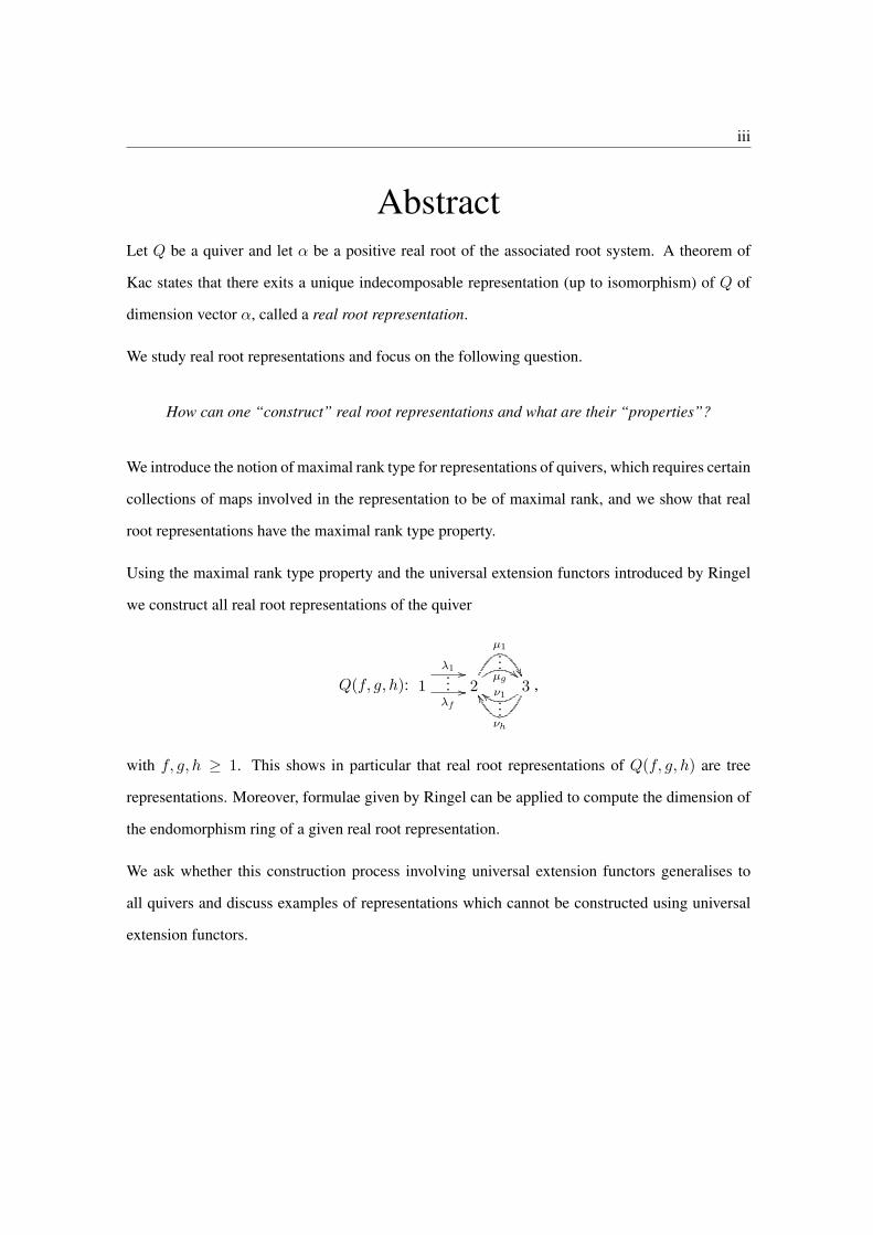
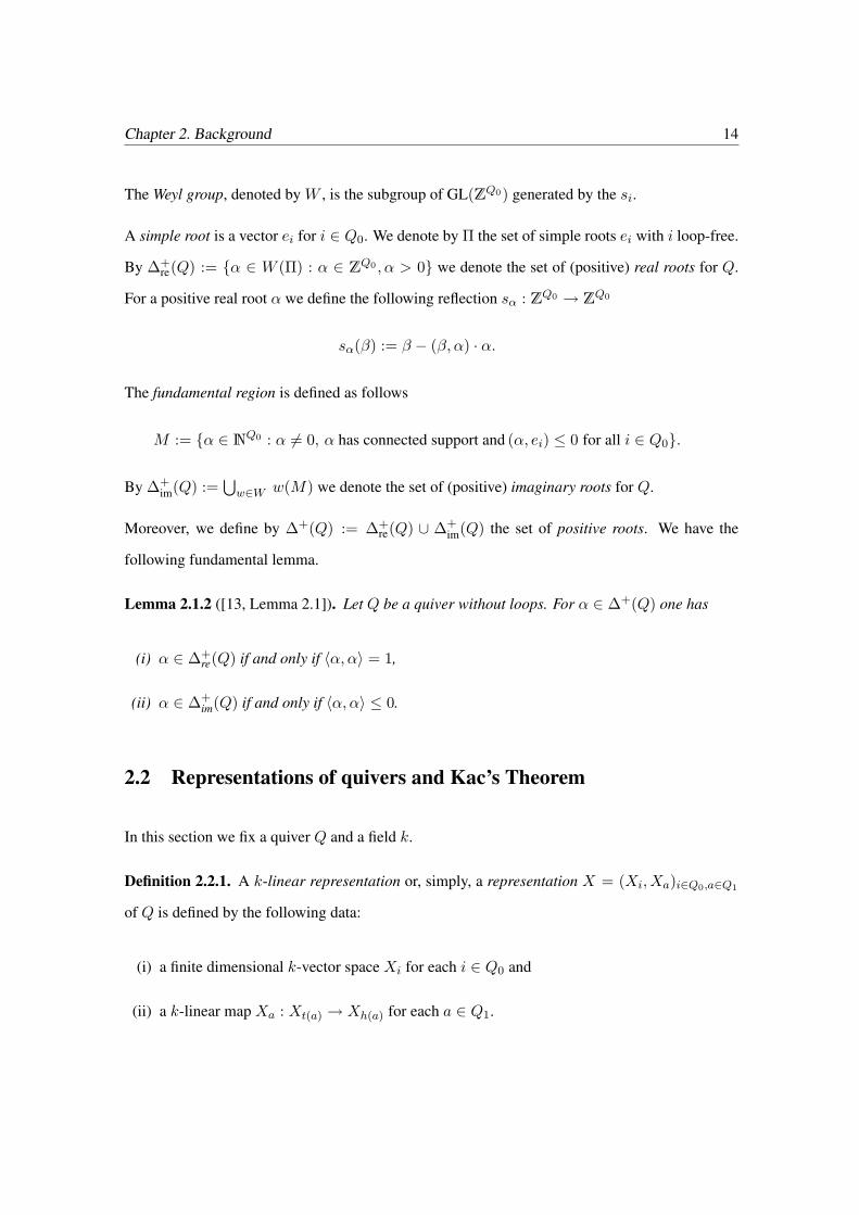
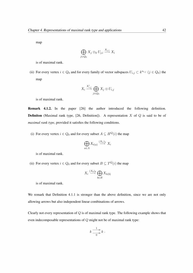
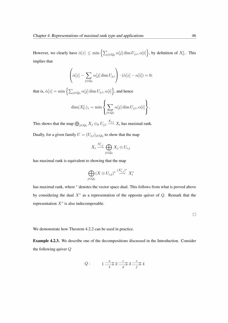
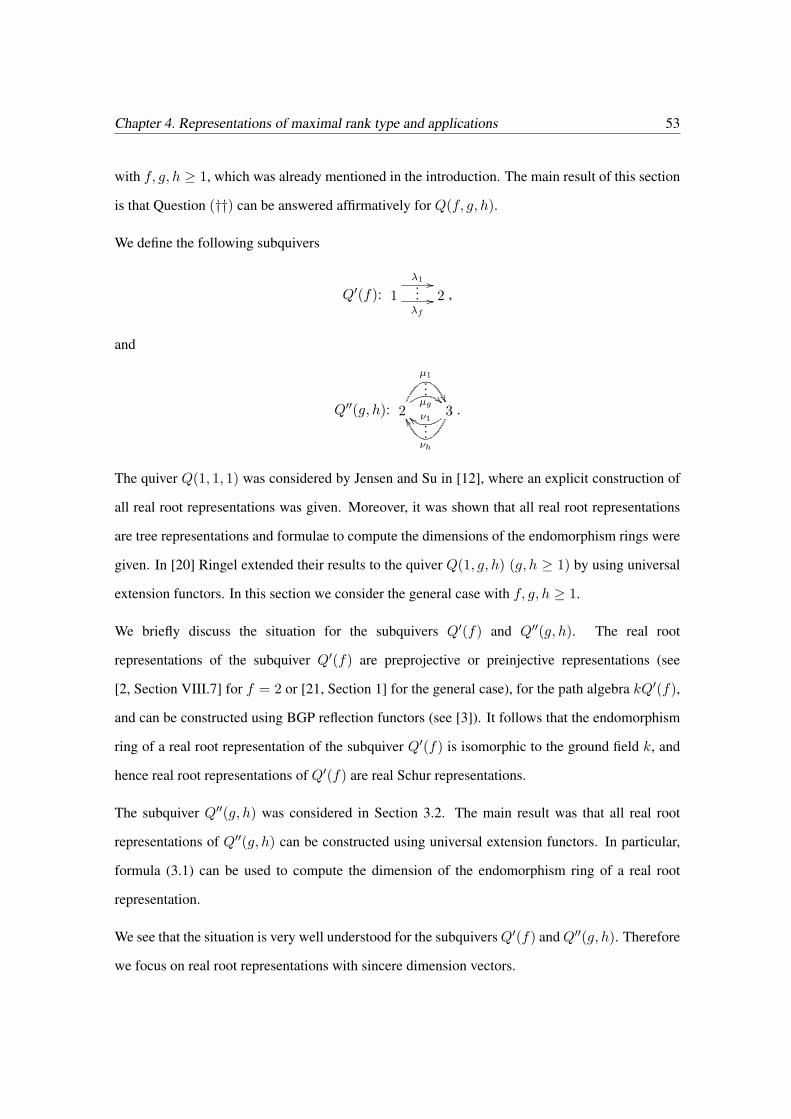
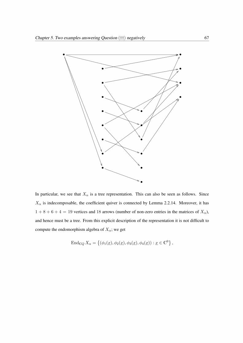
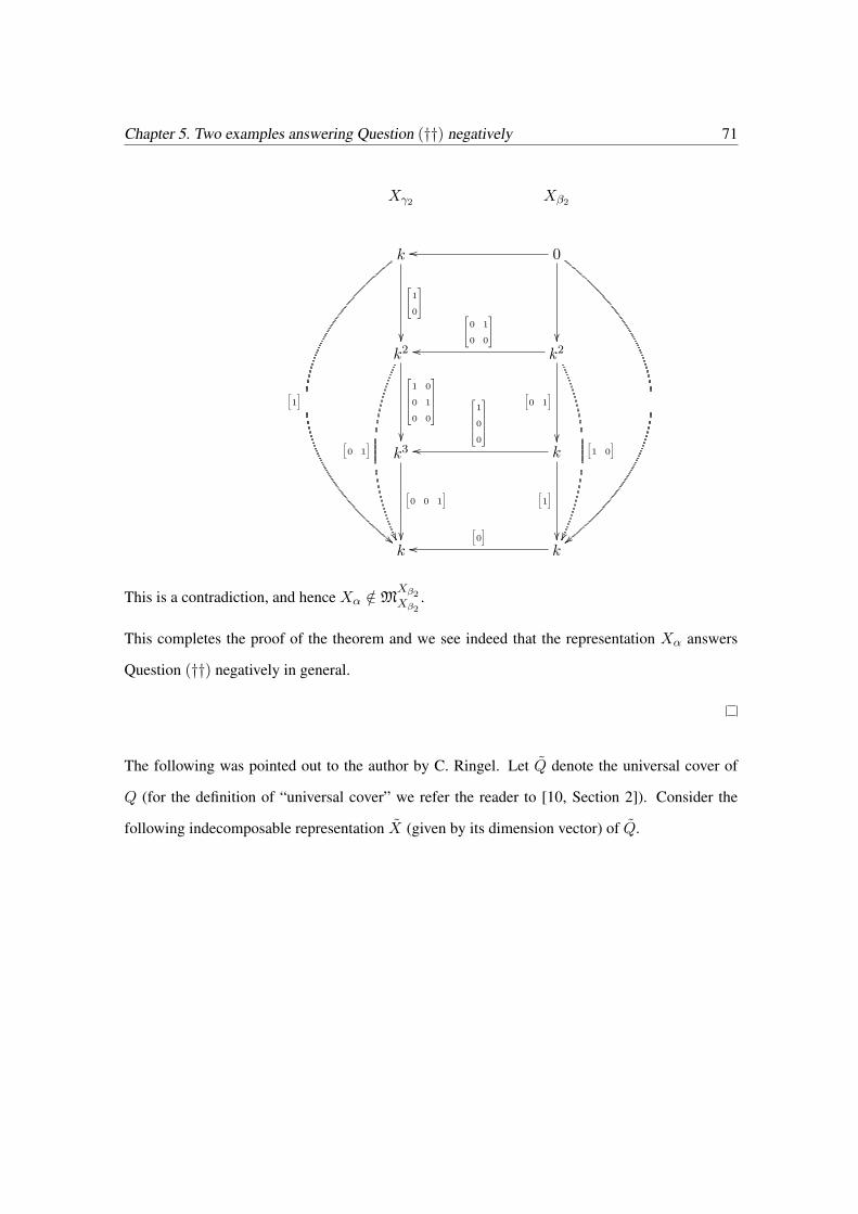
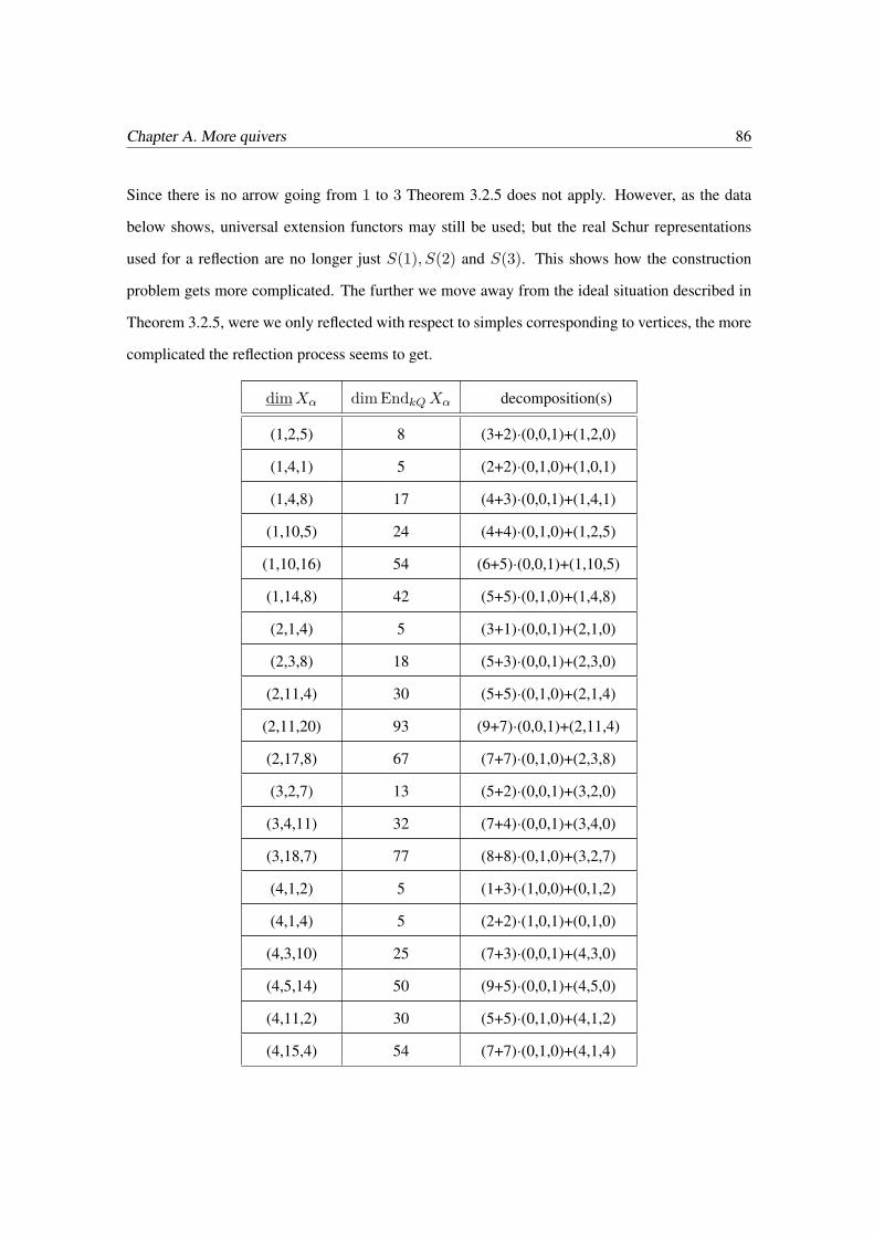
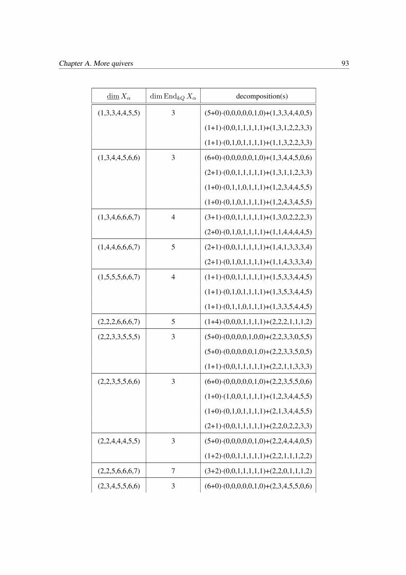
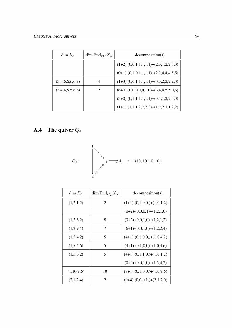
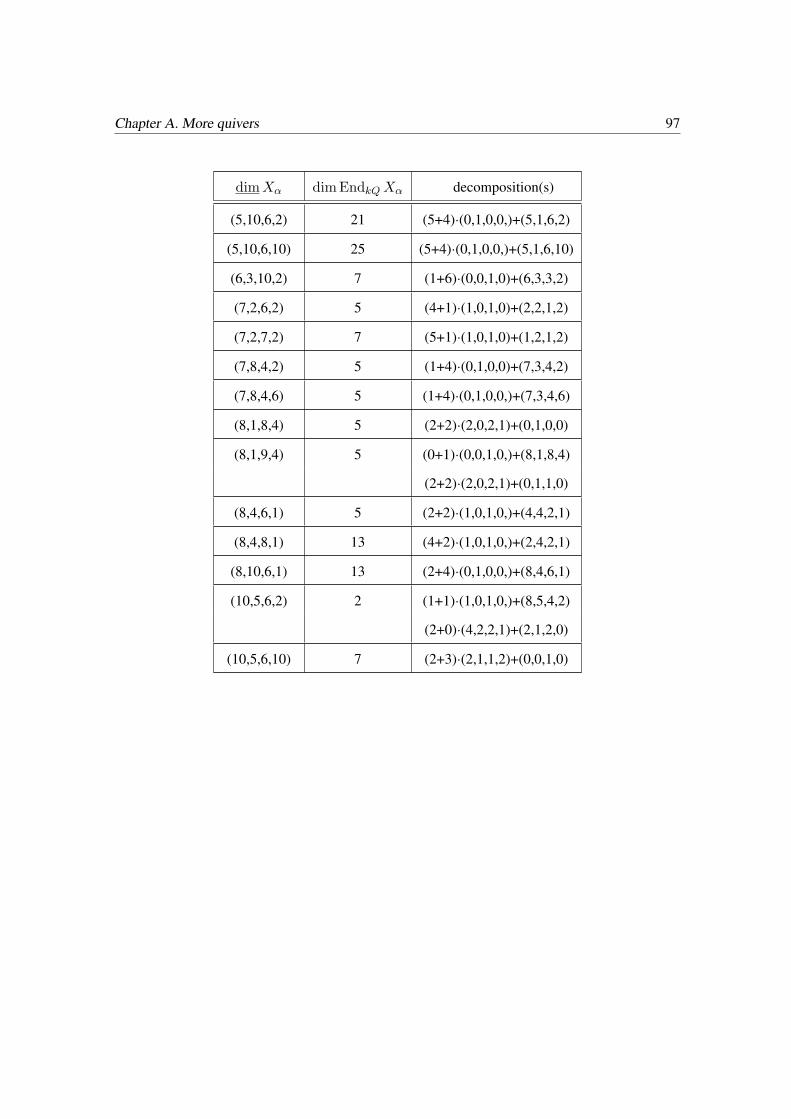
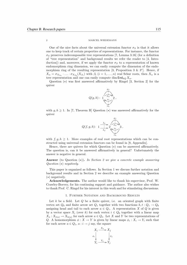
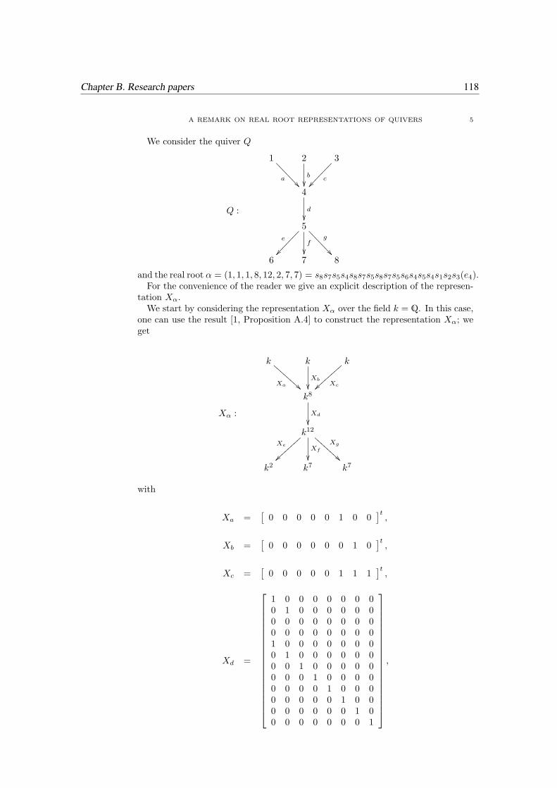
Cambridge Stud. Adv. Math., vol. 36, Cambridge Univ. Press, 1995.
[3] I.N. Bernstein, I.M. Gelfand, and V.A. Ponomarev, Coxeter functors and Gabriel’s theorem,
Uspehi Mat. Nauk 28 (1973), 19–33.
[4] K. Bongartz and P. Gabriel, Covering spaces in representation-theory, Invent. Math. 65
(1981).
[5] W.W. Crawley-Boevey, Lectures on representations of quivers, lecture notes,
http://www.maths.leeds.ac.uk/˜pmtwc/.
[6] W.W. Crawley-Boevey, More lectures on representations of quivers, lecture notes,
http://www.maths.leeds.ac.uk/˜pmtwc/.
[7] W.W. Crawley-Boevey, Geometry of the moment map for representations of quivers,
Compositio Math. 126 (2001), 257–293.
[8] W.W. Crawley-Boevey and M. Holland, Noncommutative deformations of Kleinian
singularities, Duke Math. J. 92 (1998), 605–635.
[9] V. Dlab and C.M. Ringel, Indecomposable representations of graphs and algebras, Mem.
Amer. Math. Soc. 173 (1976).
BIBLIOGRAPHY 123
[10] P. Gabriel, The universal cover of a representation-finite algebra, Representations of
Algebras, Lecture Notes in Mathematics 903, 68–105.
[11] P. Gabriel, Unzerlegbare Darstellungen I, Manuscripta Math. 6 (1972), 71–103.
[12] B.T. Jensen and X. Su, Indecomposable representations for real roots of a wild quiver, J.
Algebra 319 (2008), 2271–2294.
[13] V.G. Kac, Infinite root systems, representations of graphs and invariant theory, Invent. Math.
56 (1980), 57–92.
[14] V.G. Kac, Infinite root systems, representations of graphs and invariant theory, J. Algebra
78 (1982), 141–162.
[15] V.G. Kac, Root systems, representations of quivers and invariant theory, Invariant Theory
(Montecatini 1982), Lecture Notes in Math., vol. 996, Springer, 1983.
[16] S. Lang, Algebra, 3rd ed., Addison-Wesley, 1993.
[17] C.M. Ringel, Representations of K-species and bimodules, J. Algebra 41 (1976), 269–302.
[18] C.M. Ringel, Reflection functors for hereditary algebras, J. London Math. Soc. 21 (1980),
465–479.
[19] C.M. Ringel, Exceptional modules are tree modules, Linear Algebra Appl. 275/276 (1998),
471–493.
[20] C.M. Ringel, The real root modules for some quivers, Preprint (2006), http://www.math.uni–
bielefeld.de/ ringel/publ–new.html.
[21] A. Schofield, The internal structure of real Schur representations, Preprint (1990).
[22] A. Schofield, The field of definition of a real representation of Q, Proc. American Math. Soc.
116 (1992), 293–295.
[23] A. Schofield, General representations of quivers, Pro. London Math. Soc. 65 (1992), 46–64.
BIBLIOGRAPHY 124
[24] C. A. Weibel, An introduction to homological algebra, Cambridge Stud. Adv. Math., vol. 38,
Cambridge Univ. Press, 1994.
[25] M. Wiedemann, A remark on the constructibility of real root representations using universal
extension functors, Preprint (2007), arXiv:0802.2803 [math.RT].
[26] M. Wiedemann, Representations of maximal rank type and an application to representations
of a quiver with three vertices, Bull. London Math. Soc. 40 (2008), 479–492.