Marching Cubes Robert Hunt

CS 525

Introduction The Marching Cubes algorithm is a method for visualizing a conceptual surface called an isosurface. An isosurface is formed from a set of points in 3 space satisfying the equation v = f(x,y,z), where v is a specific value. v is called the iso-value and remains constant at any point on the isosurface. Therefore, an isosurface can be viewed as a surface within a volume where each point has the same parametric value defined by v, a user specified iso-value. We will start with the 2d equivalent of Marching Cubes called Marching Squares and then translate those concepts over to Marching Cubes. Similar to Marching Cubes, Marching Squares creates a curve, referred to as an isocurve, from a set of points in 2 space that satisfy the equation v = f(x,y), where v is a specific value.

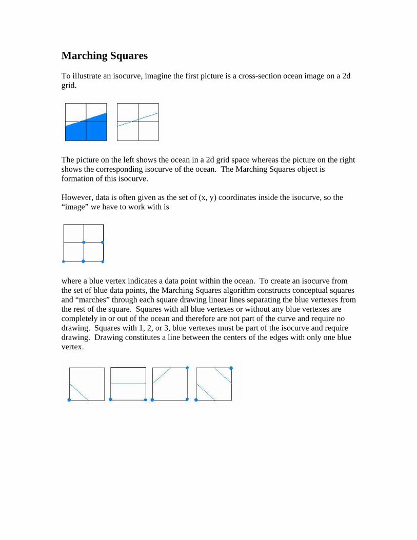
Marching Squares To illustrate an isocurve, imagine the first picture is a cross-section ocean image on a 2d grid.

The picture on the left shows the ocean in a 2d grid space whereas the picture on the right shows the corresponding isocurve of the ocean. The Marching Squares object is formation of this isocurve. However, data is often given as the set of (x, y) coordinates inside the isocurve, so the “image” we have to work with is

where a blue vertex indicates a data point within the ocean. To create an isocurve from the set of blue data points, the Marching Squares algorithm constructs conceptual squares and “marches” through each square drawing linear lines separating the blue vertexes from the rest of the square. Squares with all blue vertexes or without any blue vertexes are completely in or out of the ocean and therefore are not part of the curve and require no drawing. Squares with 1, 2, or 3, blue vertexes must be part of the isocurve and require drawing. Drawing constitutes a line between the centers of the edges with only one blue vertex.

Using this methodology, constructing an isocurve from our 2d image of the ocean looks like this:

Not a great fit, but we’ll discuss shrinking the grid size for improved accuracy later. Right now, let’s look at a larger example. Instead of an ocean, we will look at a circle. Our criteria for a curve this time will be vertexes within a circle, so the optimal result would be an isocurve matching the circle exactly. The first picture shows a black circle in a 2d grid with vertexes inside the circle indicated by the color green. The second picture shows red vertexes where lines will connect the edges to form portions of the isocurve. Finally, the last picture shows the isocurve formed by all the lines between red vertexes.

Now that you have an intuitive feel for how Marching Squares works, I’ll layout a more structured approach to use for implementation.

Structured Marching Squares Approach Step 1: Since each square has up to 4 vertexes in or out of the curve in question, 24 = 16 squares are possible.

For each vertex combination, 1 line, 2 lines, or no lines should be drawn between the edge centers of the square. Create a table (referred to as the edge table) that maps each vertex combination to edges intersecting the isocurve. index e1 e2 e3 e4edgeTable = 0000 0 0 0 0 0001 1 0 0 1 0010 1 1 0 0 0011 0 1 0 1 : : : : : 1111 0 0 0 0

Step 2: Read in two adjacent data lines to form “squares” and commence “marching” through the row of squares.

(x, y+1) (x+n, y+1)

(x, y) (x+n, y)

Step 3: At each square, assign a 1 to each vertex within the surface and a 0 to those outside. Assign these values in a square index.

index = v4 v3 v2 v1 Step 4: Using the edge table and square index, get the edges to draw lines between (i.e. edgeTable[index] = drawLines). Step 5: Draw line(s) between edges if applicable. Step 6: Go to next square.

Pseudo Code: Create an edge table Read a line of data while(moreDataLines) {

Read in next line of data while(moreSquares) {

Fill square index (Assign 1 or 0 to index elements for each vertex) edgesToDrawBetween = edgeTable[squareIndex]

Draw lines using edgesToDrawBetween currentSquare++;

} Discard data line }

Vertex Combination Simplifications Through symmetries, the 24 vertex combinations reduce to 5. The first symmetry is complement vertex combinations produce the same line for combinations with adjacent vertexes.

For nonadjacent vertexes, this symmetry does not hold.

The second symmetry is rotational symmetry.

These symmetrical relationships are not too important in Marching Squares since only 16 total square possibilities exist, but they become very important in Marching Cubes. The final 5 unique squares are below.

Non-Boolean Data Sets Up to this point, we’ve concerned ourselves only with vertexes being inside or outside of a criterion. If an edge had a one vertex inside and the other outside the criteria, the isocurve crossed the middle of the edge. However, vertexes can hold specific numeric values beyond the Boolean value of in or out. Those values could conceptually represent anything, a color, substrate density, type of body tissue, etc. As one would suspect, however, when we add values to the edge vertexes, the vertex for the isocurve intersection should cross closer to the vertex with the value closest to the threshold criteria. Let’s look at an example. Imagine a threshold criterion of less than 32° Fahrenheit and data values at each vertex indicating the degrees Fahrenheit at that point in the 2d space.

Using our previous method on this square, we would get the following.

Clearly, the isocurve line should go closer to the vertex with a value of 30° F than the vertex with 50° F, but the drawn line puts equal distance from the isocurve intersection and each vertex.

Linearly interpolating between the two vertexes solves this problem and gives a result similar to the following. Notice how the isocurve is pulled closer to the bottom vertex.

The formula for linear interpolation is: vi = va + (t – da) [(vb – va) / (db – da)], where

vi is the isocurve intersection vertex, t is the threshold value, va is the vertex below t, vb is the vertex above t, da is the data at va, and db is the data at vb.

Looking at the formula, the term [(vb – va) / (db – da)] generates a ratio of edge length per unit data. This ratio maps data values to edge length values. So (t – da) gives the difference in data units between the intersection vertex and the vertex inside the isocurve. Multiplying that difference by the ratio gives us the distance vi is from va, and since we started at va, we add va to that distance, which gives us the point vi. In our example, let’s assume v1 is at (0, 0), and v4 is at (0, 10). We know the vix will be 0, so we only need concern ourselves with viy.

viy = 0 + (32 – 30) [(10 – 0) / (50 – 30)] = 1 Therefore, the intersection of the isocurve on the edge between (0, 0) and (0, 10) should be (0, 1), which is much closer to v1 than v4. Incidentally, swapping a and b variables will produce the same vertex.

viy = 10 + (32 – 50) [(0 – 10) / (30 – 50)] = 1 In other words, va could just as easily represented a vertex outside and vb a vertex inside the isocurve.

Marching Cubes The time for 3d has finally come, and with the Marching Squares principles translating over, the shift should be relatively smooth one. Logically, we move from squares to cubes.

index = v4 v3 v2 v1 From isocurves, we move to isosurfaces. Thus, we will no longer be connecting 2 edges with lines, but instead be connecting 3 edges to form triangles.

Recall in Marching Squares, each square could have up to 4 vertexes in or out of the isocurve in question, which led to 24 possible squares. A cube, however, has 8 vertexes, which leads to 28, or 256, drawing possibilities. Luckily, by using the same symmetries discussed for Marching Squares (which probably seemed like overkill at the time), we can considerably reduce that 256. Vertex combinations and their complements produce the same triangle(s) facets, so 256 permutations can be reduced to 128. Through rotational symmetry, inspection can further condense the triangle facet combinations from 128 to 15 patterns.

index = v7 v6 v5 v4 v3 v2 v1 v0

In the 15 cube combinations, the number of triangular surfaces drawn range from 0 to 4. Therefore, our edge table will now have 12 columns per entry, enough room for 4 triangles requiring 3 vertexes each. Recall, however, the edge table returns edges containing the triangles vertexes, not the vertexes themselves. A triangle vertex is calculated by linear interpolation of the two vertexes of the intersecting edge. Pseudo Code: Create an edge table Read in 3 2d slices of data while(moreDataSlices) {

Read in next slice of data while(moreCubes) {

Fill cube index (Assign 1 or 0 to index elements for each vertex) edgesToDrawBetween = edgeTable[cubeIndex]

Interpolate triangle vertexes from edge vertexes Determine triangle vertex normals

Draw triangle(s) currentCube++;

} Discard data slice }

On top of the obvious modifications made to the pseudo code to transform it from a 2d Marching Squares to a 3d Marching Cubes, you’ll notice two interesting and unexpected additions. Instead of reading in 2 2d slices of data, which would be analogous to reading in 2 1-d lines of data in Marching Squares, we read in 4 slices. The other addition is calculation of normals at the triangle vertexes. The additions are related in that to calculate the normals at the triangle vertexes you need to incorporate the normals of all triangles using that vertex, not just the triangles in the current cube. With the inclusion of vertex normals in rendering, we can smooth shade the output with Gouraud shading.

Grid Size A key factor to image quality and speed of calculation is grid size. A decrease in grid will increase the time of surface construction but amplify the surface detail. Look at the following renderings of “bobby molecules” generated at different grid sizes.

Notice the first picture with a grid size of 10. The neck of the “bobby molecule” fits completely inside the cube volume and therefore not drawn. Incidentally, for those wondering if a higher degree of interpolation for triangle vertexes would further improve image quality, experimentation has shown little enhancement. Applications Although employed in many arenas, isosurface creation is heavily utilized in medical visualization. Isosurfaces recreate the digitized images taken by computed tomography (CT), magnetic resonance (MR), and single-photon emission computed tomography.