Marcin Waniek Tomasz Michalak Michael Wooldridge address the above question from an individual’s...

Hiding Individuals and Communities in a Social Network

Marcin WaniekUniversity of Warsaw

[email protected]

Tomasz MichalakUniversity of Oxford

& University of Warsaw

[email protected]

Talal RahwanMasdar Institute

of Science and Technology

[email protected]

Michael WooldridgeUniversity of Oxford

[email protected]

Abstract

The Internet and social media have fueled enormous interest in social network analysis. New tools continue tobe developed and used to analyse our personal connections, with particular emphasis on detecting communities oridentifying key individuals in a social network. This raises privacy concerns that are likely to exacerbate in the future.With this in mind, we ask the question: Can individuals or groups actively manage their connections to evade socialnetwork analysis tools? By addressing this question, the general public may better protect their privacy, oppressedactivist groups may better conceal their existence, and security agencies may better understand how terrorists escapedetection. We first study how an individual can evade “network centrality” analysis without compromising his or herinfluence within the network. We prove that an optimal solution to this problem is hard to compute. Despite thishardness, we demonstrate that even a simple heuristic, whereby attention is restricted to the individual’s immediateneighbourhood, can be surprisingly effective in practice. For instance, it could disguise Mohamed Atta’s leading positionwithin the WTC terrorist network, and that is by rewiring a strikingly-small number of connections. Next, we studyhow a community can increase the likelihood of being overlooked by community-detection algorithms. We propose ameasure of concealment, expressing how well a community is hidden, and use it to demonstrate the effectiveness ofa simple heuristic, whereby members of the community either “unfriend” certain other members, or “befriend” somenon-members, in a coordinated effort to camouflage their community.

1 Introduction

The on-going process of datafication continues to turnmany aspects of our lives into computerised data [23].This data is being collected and analysed for various di-verse applications by public and private institutions alike.One particular type of data that has received significantattention over the past decade concerns our social con-nections. To this end, a number of tools have been advo-cated for social network analysis, with particular empha-sis on the detection of communities or the identificationof key individuals within a network. For all their benefits,the widespread use of such tools raises legitimate privacyconcerns. For instance, Mislove et al. [24] demonstratedhow, by analysing Facebook’s social network structure,

as well as the attributes of some users, it is possible toinfer otherwise-private information about other Facebookusers.

To tackle such privacy issues, various countermeasureshave been proposed, ranging from strict legal controls [1],through algorithmic solutions [15], to market-like mech-anisms that allow participants to monetize their personalinformation [20]. However, to date only few such counter-measures have been implemented, leaving the privacy is-sue largely unresolved, e.g., as is evident from the very re-cent release of Facebook’s “Global Government RequestsReport” [2], which revealed a global increase in govern-ment requests to secretly access user data. Furthermore, itis unlikely that effective legal mechanisms will be intro-duced in countries with authoritarian regimes, where so-

1

arX

iv:1

608.

0037

5v1

[cs

.SI]

1 A

ug 2

016

cial networking sites and other internet content is policed,and anti-governmental blogs and activities are censored[17, 18].

Against this background, we ask the question: can in-dividuals or communities proactively manage their so-cial connections so that their privacy is less exposed tothe workings of network analysis tools? To put it differ-ently, can we disguise our standing in the network to es-cape detection? This matters because, on one hand, it as-sists the general public in protecting their privacy againstintrusion from government and corporate interests; onthe other hand, it assists counterterrorism units and law-enforcement agencies in understanding how criminalsand terrorists could escape detection, especially giventheir increasing reliance of social-media survival strate-gies [27, 14]. To date, however, this fundamental ques-tion has received little attention in the literature, as mostresearch efforts have focused on developing ever more so-phisticated network analysis tools, rather than consideringhow to evade them.

To address the above question from an individual’sviewpoint, we focus on three main centrality measures,namely degree, closeness, and betweenness, and studyhow one can avoid being highlighted by those measureswithout compromising his or her influence. Since, from agraph-theoretic perspective, this is fundamentally an opti-mization problem, we analyse its computational complex-ity to illuminate the theoretical limits of such capabilityas disguising oneself. Although we show that an optimalsolution is often hard to compute, we demonstrate the ef-fectiveness of a surprisingly simple heuristic, whereby therewiring of social connections is restricted to the individ-ual’s immediate network neighbourhood. Specifically, itinvolves two actions that are already available on popularsocial-media platforms: (i) “unfriending” certain neigh-bours; (ii) introducing certain neighbours to each other.

From a group’s viewpoint, we study how a commu-nity can conceal itself to increase the likelihood of beingoverlooked by community-detection algorithms. To thisend, we propose a measure of concealment, designed toquantify the degree to which a group of individuals is hid-den. Using this measure, we demonstrate the effective-ness of yet another simple heuristic, whereby members ofthe community either “unfriend” certain other members,or “befriend” some non-members to blend into the sur-rounding web of social connections.

2 The ModelThis section presents the basic concepts and objectives;all formal definitions can be found in the Supporting In-

formation.

Centrality Measures: A measure of centrality reflectsthe importance of any given node in the network. Ar-guably, the standard centrality measures are: degree,closeness and betweenness [11]. In particular, for anygiven node v, the degree centrality focuses on the numberof neighbours that v has (the more neighbours the better).In contrast, the closeness centrality quantifies the impor-tance of v based on its average distance to other nodes(the closer the better). Finally, the betweenness centralityfocuses on the number of shortest paths on which v lies(the more paths the better).

Models of Influence: The best established mathemat-ical models of influence are the Independent Cascademodel [12] and the Linear Threshold model [16]. Ba-sically, both models start with some “active” subset ofnodes, called the seed set.1 Then, as time passes (in dis-crete rounds), new nodes become activated due to the in-fluence from other previously-activated nodes. The twomodels differ in the way influence propagates throughthe network. Specifically, in the Independent Cascademodel, an active node activates each of its neighbourswith some pre-defined probability. In contrast, with theLinear Threshold model, each node has some random pre-defined threshold, and gets activated when the number ofits active neighbors exceeds that threshold. Under eithermodel, the influence of a node, v, on another, w, is mea-sured as the probability that w gets activated when theseed set is {v}.First Objective: Given a network and a source node, v†,our objective is to conceal the importance of v† by de-creasing its centrality (according to each of the aforemen-tioned measures of centrality) without compromising itsinfluence over the network (according to the aforemen-tioned models of influence). We do so by rewiring thelinks of the network, without exceeding a certain bud-get—the maximum number of links allowed to be mod-ified (i.e., added or removed). To simplify our analysis,we divide the process of disguising v† into two consecu-tive phases. In the first phase, part of the budget is spenton minimizing the three centrality measures, during whichthe influence of v† is likely to decrease—we call this thecentrality minimization problem. The second phase in-volves spending the remaining budget to recover as muchas possible of the influence of v† while avoiding the addi-tion of any links that were removed during the centrality

1An active node can be thought of as an infected person who influ-ences, but not necessarily infects, his or her neighbours. Analogously,an inactive node can be a healthy person who is influenced by any in-fected neighbours he or she may have; stronger influence corresponds tostronger chances of infection.

2

minimization phase. Here, we consider two variants ofthis latter problem: (i) the individual influence recoveryproblem, where the goal is to recover the influence of v†

over every single node, and (ii) the global influence re-covery problem, where the goal is to recover the sum ofinfluences of v† over all nodes.

Second Objective: Given a community, i.e., subset ofnodes, C†, our goal is the conceal the identity of C† byhiding its existence within the network. Recall that a com-munity structure is a partition of the set of nodes into dis-joint and exhaustive subsets, or “communities”. As such,C† is exposed if a community-detection algorithm is ableto return a community structure, CS , such that C† ∈ CS .We hide C† by rewiring the links of the network, againaccording to some budget, i.e., maximum number of per-mitted modifications.

3 Disguising Individuals

3.1 Hardness ResultsOur main theoretical results are summarized in Table 1(for more details, see theorems 1 through 4 in the Support-ing Information). As shown in the table, all the problemsunder consideration turn out to be NP-complete, with theexception of minimizing degree centrality. To put it dif-ferently, finding an optimal way to disguise one’s impor-tance in a social network is extremely difficult (from acomputational point of view), not to mention the fact thatit requires knowing the entire network structure, and mayalso require adding or removing links that are far from thesource node.

Disguising centrality (Degree) PDisguising centrality (Closeness) NPCDisguising centrality (Betweenness) NPCIndividual influence recovery (LT) NPCIndividual influence recovery (IC) NPCGlobal influence recovery (LT) NPCGlobal influence recovery (IC) NPC

Table 1: Summary of our computational-hardness results.

3.2 A Scalable HeuristicTypically, one has very limited knowledge of the socialties beyond his or her immediate friends, or maybe friendsof friends. However, even if one was able to somehow ac-quire information about the entire network structure, ourtheoretical results from the previous subsection suggest

that it is extremely unlikely for such an individual to havethe necessary computational power to optimally disguisehimself or herself. Against this background, we inves-tigate the possibility of disguising one’s centrality ade-quately (albeit not optimally) while restricting one’s at-tention to only his or her immediate neighbourhood, andwithout requiring massive computational power nor ex-pertise in sophisticated optimization techniques. With thisin mind, we propose a heuristic whose instructions aresimple enough for an average user of social-networkingservices to understand and use, regardless of their techni-cal background. Our heuristic, called ROAM—RemoveOne, Add Many—is detailed in the box below, and an il-lustration of how it works is presented in Figure 1.

The ROAM heuristic given a budget b:• Step 1: Remove the link between the source

node, v†, and its neighbour of choice, v0;

• Step 2: Connect v0 to b − 1 nodes of choice,who are neighbours of v† but not of v0 (if thereare fewer than b − 1 such neighbours, connectv0 to all of them).

Let us now comment on this heuristic, starting withStep 1. As far as the centrality of v† is concerned, thisstep can only be beneficial. More specifically, cutting offv† from one of its neighbours is the only way to reducethe degree of v†. Likewise, Step 1 can only decrease thecloseness of v† (this happens when all shortest paths be-tween v† and some other node run through the removedlink), and can only decrease the betweenness of v† (thishappens when some of the shortest paths going throughv† contain the removed link). However, as far as the in-fluence of v† is concerned, Step 1 may be detrimental, asit deprives v† from its direct influence over v0.

Moving on to Step 2, this step is primarily designed tocompensate for any influence that v† may have lost dur-ing the previous step. Specifically, it creates new, indi-rect connections between v† and v0 to compensate for thedirect one that was removed earlier. As far as the cen-trality of v† is concerned, while Step 2 does not affectthe degree of v†, it increases the degrees of some of itsneighbours, which in turn contributes towards concealingthe relative importance of v† within the network. Further-more, the addition of a link, (v0, vi)—where vi is someneighbour of v†—cannot increase the closeness centralityof v† beyond its original state, i.e., its state before runningthe ROAM heuristic altogether. This is because any pathcontaining (v0, vi) and (vi, v

†) is certainly longer than anoriginal path in which (v0, vi) and (vi, v

†) were replacedwith (v0, v

†). Likewise, the addition of this link cannot

3

9

8

7

10

30

32363326

34

35

24

11

29

23

1222

1815

2827

12

14

13

19

17

3

4

20

31

5

9

8

7

10

30

32363326

34

35

24

11

29

23

1222

1815

2827

12

14

13

19

17

3

4

20

31

5

9

8

7

10

30

32363326

34

35

24

11

29

23

1222

1815

2827

12

14

13

19

17

3

4

20

31

5

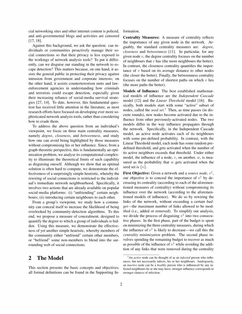
6Original networkMohamed Atta1st in Degree centrality ranking1st in Closeness centrality ranking1st in Betweenness centrality rankingIC influence = 2.55LT influence = 6.44

6After two executions of our heuristicMohamed Atta5th in Degree centrality ranking4th in Closeness centrality ranking11th in Betweenness centrality rankingIC influence = 2.21LT influence = 6.90

6After one execution of our heuristicMohamed Atta3rd in Degree centrality ranking2nd in Closeness centrality ranking5th in Betweenness centrality rankingIC influence = 2.39LT influence = 6.72

6 66

25 2525

16 1616

21 2121

Figure 1: Executing the ROAM heuristic twice on the 9/11 terrorist network to hide Mohamed Atta—one of theringleaders of the attack [19]. The red link is the one to be to removed by the algorithm, and the dashed links are theones to be added.

increase the betweenness centrality of v† beyond its orig-inal state, because replacing a direct connection betweenv† and v0 with an indirect one cannot increase the per-centage of shortest paths going through v†.

Finally, let us comment on the how to choose v0, andhow to choose the neighbours of v† to connect to v0.Based on the simulation study reported in the Support-ing Information, we choose v0 to be the neighbour ofv† with the most connections, and we connect v0 to theb − 1 neighbours of v† with the least connections. Withsuch choices, it is relatively straightforward to execute theROAM heuristic on existing social-networking services.On Facebook, for example, one can typically view thenumber of friends that each of his friends has (even ifsome of them make this information private, one can stillchoose among those that do not). Once the nodes are cho-sen, Step 1 simply requires v† to “unfriend” v0, whereasStep 2 requires v† to “suggest” the friendship of v0 to theother chosen nodes. Note that, on Facebook, v† can onlyintroduce two individuals to each other if they were bothv†’s friends. As such, Step 2 must be executed beforeStep 1, that is, v† must end the friendship with v0 afterintroducing v0 to the other nodes.

4 Disguising Communities

4.1 A Measure of Concealment

We propose a measure of how well a community, C†, ishidden in a community structure, CS . Note that C† isnot necessarily a member of CS . To put it differently,when describing C† as a “community”, we mean to usethis term in its broader sense, where C† is essentially just

a subset of nodes. As such, when measuring how well C†

is hidden in CS , it may well be the case that the membersof C† are spread out across multiple communities in CS .

To this end, we start by proposing two measures, de-noted by µ′ and µ′′, which capture different aspects ofconcealment. In particular, µ′ is defined for every com-munity C† ⊆ V and every community structure CS asfollows:

µ′(C†,CS ) =|{Ci ∈ CS : Ci ∩ C† 6= ∅}|−1

max(|CS |−1, 1)maxCi∈CS (|Ci ∩ C†|).

Basically, this measure focuses on how well the membersof C† are spread out across the communities in CS . Inmore detail, we have µ′(C†,CS ) ∈ [0, 1], and the greaterµ′(C†,CS ), the greater the concealment of C† in CS .Note that the numerator grows linearly with the numberof communities that C† is distributed over. Subtracting1 from both the numerator and the |CS | term of the de-nominator is meant to handle the worst case, where allmembers of C† appear in a single (possibly larger) com-munity in CS ; in this case, we have: µ′(C†,CS ) = 0.In contrast, the term maxC∈CS (|C ∩ C†|) is meant topromote community structures in which the members ofC† are more evenly distributed across the communitiesin CS . As such, the maximum concealment is achievedwhen the members of C† are uniformly distributed, witheach member appearing in a separate community; in thiscase: µ′(C†,CS ) = 1.

Moving on to the second measure, µ′′, it is defined as:

µ′′(C†,CS ) =∑

Ci∈CS

|Ci \ C†|max(n− |C†|, 1)

.

Intuitively, µ′′ focuses on how well C† is “hidden in

4

(a) 𝜇(𝐶†,𝐶𝑆) = 0 (b) 𝜇(𝐶†,𝐶𝑆) =3

8(c) 𝜇(𝐶†,𝐶𝑆) =1

𝐶† 𝐶† 𝐶†

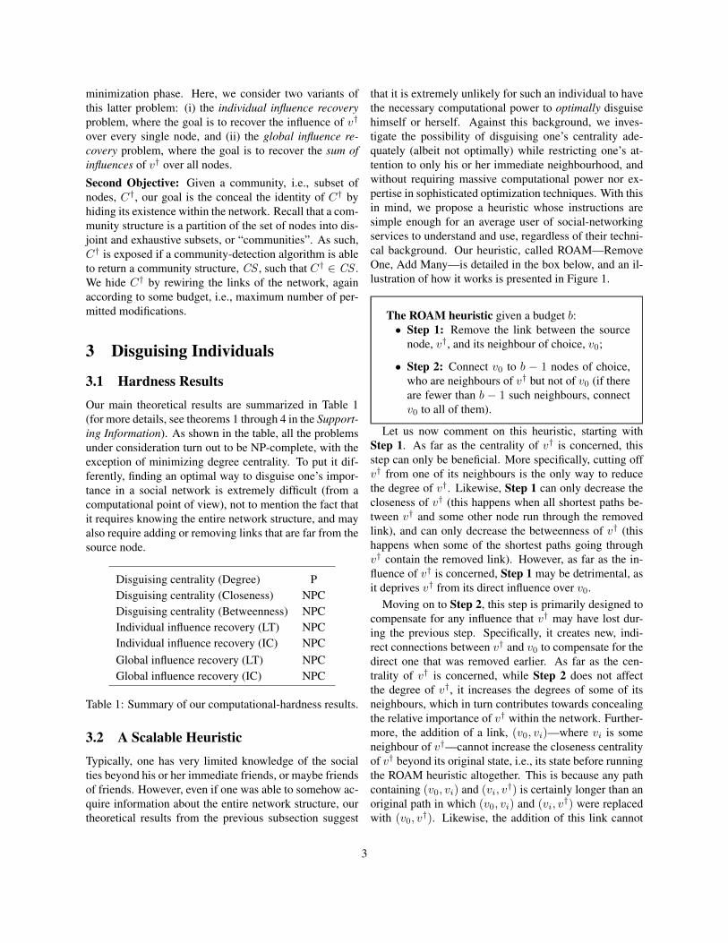
Figure 2: How the concealment of C† differs from onecommunity structure to another according to µwhere α =0.5.

the crowd”; it grows linearly with the number of non-members of C† that appear with members of C† in thesame community in CS . Note that µ′′(C†,CS ) ∈ [0, 1],and the greater the value, the greater the concealment ofC† in CS .

Having defined µ′ and µ′′, we now use the two asbuilding blocks to construct a single measure whereby thetrade-off between µ′ and µ′′ is controlled by a parameter,α ∈ [0, 1]. More formally, our proposed measure of con-cealment of a communityC† in a community structure CSis:

µ(C†,CS ) = αµ′(C†,CS ) + (1− α)µ′′(C†,CS ).

Figure 2 presents a sample network with three differ-ent community structures, and highlights the communitythat we wish to conceal, namely C†. For every such com-munity structure, we measure the concealment of C† us-ing our measure µ with α = 0.5. In particular, Fig-ure 2(a) presents one extreme where µ(C†,CS ) = 0, re-flecting the fact that C† is completely exposed as a com-munity. Figure 2(b) presents the other extreme whereµ(C†,CS ) = 1, reflecting the fact that C† is completelyhidden, since every member appears in a separate com-munity along some non-member ofC†. Finally, a case be-tween the two extremes is presented in Figure 2(c), whereµ(C†,CS ) = 3

8 .

4.2 A Scalable Heuristic

We set to develop a simple heuristic that can be appliedby any group of people regardless of their technical back-ground or their knowledge of the network topology. Af-ter all, it is of little use to have an exact algorithm thatcan only be understood or applied by optimization expertsarmed with enormous processing power. Likewise, exactalgorithms that require knowing the entire network topol-ogy may prove useless, since such knowledge is rarelyavailable.

Our heuristic, called DICE—Disconnect Internally,Connect Externally—is detailed in the box below.

The DICE heuristic given a budget b:• Step 1: Disconnect d ≤ b links from withinC†;

• Step 2: Connect b−d nodes from within C† tob− d nodes from outside of C†.

This heuristic is inspired by modularity [26]—a widelyused index for measuring the quality of any given com-munity structure. Specifically, it promotes structuresthat have dense connections within communities andsparse connections between them. As such, community-detection algorithms are typically designed to search fora structure that maximizes modularity. With this in mind,Step 1 of our heuristic decreases the density of the con-nections within C†, whereas Step 2 increases the connec-tions between C† and other communities. In doing so, acommunity-detection algorithm is more likely to overlookC†, i.e., it would fail to recognizeC† as a community, andinstead assign its members to multiple communities.

Finally, let us comment on how DICE can be appliedin practice. On Facebook, for example, Step 1 requiressome members to “unfriend” other members, which israther straightforward. As for Step 2, members mustsend a friendship request to non-members; these couldbe classmates, coworkers, neighbours living next door, oreven random people (it is possible to try multiple randomfriendship requests, hoping that some of them would besuccessful).

5 Experiments

5.1 Data setsWe experiment with two types of real-life networks:(a). Covert organizations: we consider three terrorist net-

work, responsible for the WTC 9/11 attacks [19];the 2002 Bali attack [13]; and the 2004 Madrid trainbombings [13];

(b). Social networks: we study anonymized fragments ofthree social networks, namely Facebook, Twitter andGoogle+. These fragments are taken from SNAP—the Stanford Network Analysis Platform [21].

We also study randomly-generated networks, namely:(a). Scale-free networks using the Barabasi-Albert model

[4]. We write ScaleFree(x, y) where x is the numberof nodes; y is the number of links added with eachnode;

5

Degree Ranking Closeness Ranking Betweenness Ranking IC Influence LT InfluenceM

adri

dbo

mbi

ng

0

5

10

15

20

0 2 4 6 8

5

10

0 2 4 6 8

0

10

20

30

40

0 2 4 6 8

0.6

0.9

1.2

1.5

0 2 4 6 8

10

15

20

0 2 4 6 8

ScaleFree(100,3)

1

2

3

4

5

0.0 2.5 5.0 7.5 10.0

2.5

5.0

7.5

10.0

12.5

0.0 2.5 5.0 7.5 10.0

2.5

5.0

7.5

0.0 2.5 5.0 7.5 10.0

0.7

0.8

0.9

1.0

0.0 2.5 5.0 7.5 10.0

0.9

1.0

1.1

1.2

1.3

0.0 2.5 5.0 7.5 10.0

Face

book

(med

ium

)

8

12

16

0 5 10 15 20

10

20

30

0 5 10 15 20

10

15

20

25

0 5 10 15 20

137

138

139

140

0 5 10 15 20

30

33

36

39

0 5 10 15 20

ROAM(2) ROAM(3) ROAM(4)

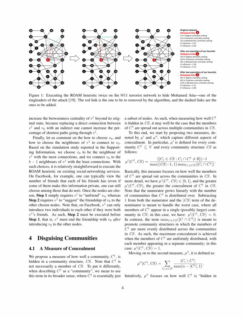
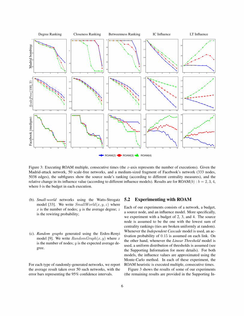
Figure 3: Executing ROAM multiple, consecutive times (the x-axis represents the number of executions). Given theMadrid-attack network, 50 scale-free networks, and a medium-sized fragment of Facebook’s network (333 nodes,5038 edges), the subfigures show the source node’s ranking (according to different centrality measures), and therelative change in its influence value (according to different influence models). Results are for ROAM(b) : b = 2, 3, 4,where b is the budget in each execution.

(b). Small-world networks using the Watts-Strogatzmodel [33]. We write SmallWorld(x, y, z) wherex is the number of nodes; y is the average degree; zis the rewiring probability;

(c). Random graphs generated using the Erdos-Renyimodel [9]. We write RandomGraph(x, y) where xis the number of nodes; y is the expected average de-gree.

For each type of randomly-generated networks, we reportthe average result taken over 50 such networks, with theerror bars representing the 95% confidence intervals.

5.2 Experimenting with ROAMEach of our experiments consists of a network, a budget,a source node, and an influence model. More specifically,we experiment with a budget of 2, 3, and 4. The sourcenode is assumed to be the one with the lowest sum ofcentrality rankings (ties are broken uniformly at random).Whenever the Independent Cascade model is used, an ac-tivation probability of 0.15 is assumed on each link. Onthe other hand, whenever the Linear Threshold model isused, a uniform distribution of thresholds is assumed (seethe Supporting Information for more details). For bothmodels, the influence values are approximated using theMonte-Carlo method. In each of these experiment, theROAM heuristic is executed multiple, consecutive times.

Figure 3 shows the results of some of our experiments(the remaining results are provided in the Supporting In-

6

((b = 4, d = 0) (b = 4, d = 4)M

adri

dbo

mbi

ng

●

●

●●

●● ●

●

●

●

●

0.0

0.1

0.2

0.3

0.4

0.00 0.25 0.50 0.75 1.00

● ●

●

●

●●●

●

●●●0.0

0.2

0.4

0.00 0.25 0.50 0.75 1.00

ScaleFree(100,3)

●

● ●

●●●

●

●●

●

●

0.0

0.1

0.2

0.3

0.4

0.00 0.25 0.50 0.75 1.00

●

●

●●

●

●

●

●●

● ●

0.0

0.2

0.4

0.00 0.25 0.50 0.75 1.00

Face

book

(med

ium

)

0.0

0.1

0.2

0.3

0.00 0.25 0.50 0.75 1.00

0.0

0.1

0.2

0.3

0.00 0.25 0.50 0.75 1.00

●edgeBetweenness

fastGreedy

infomap

leadingEigen

louvain

spinglass

walktrap

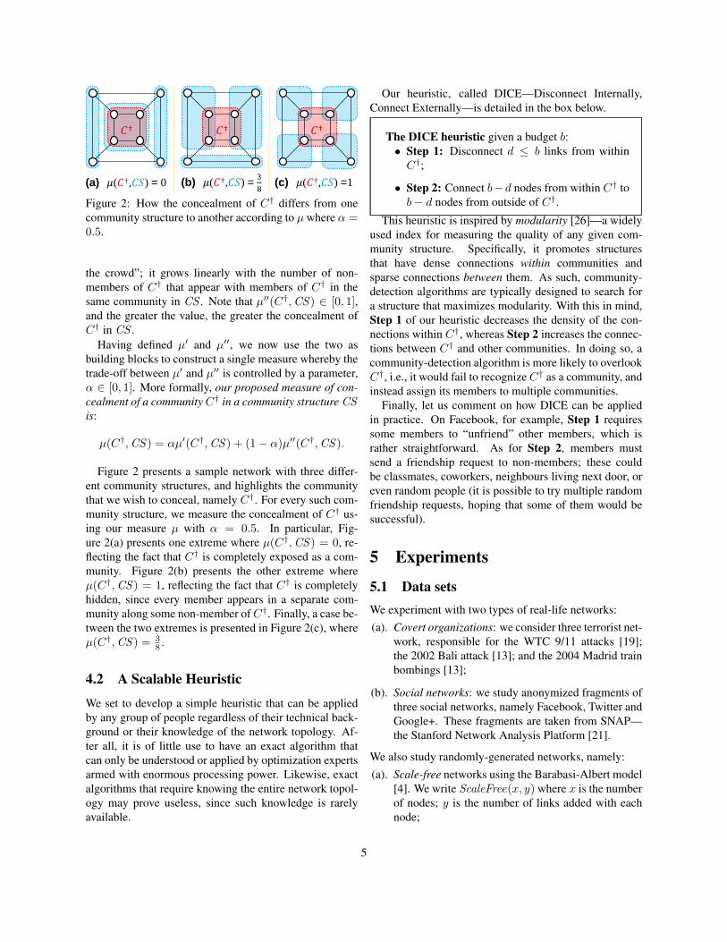
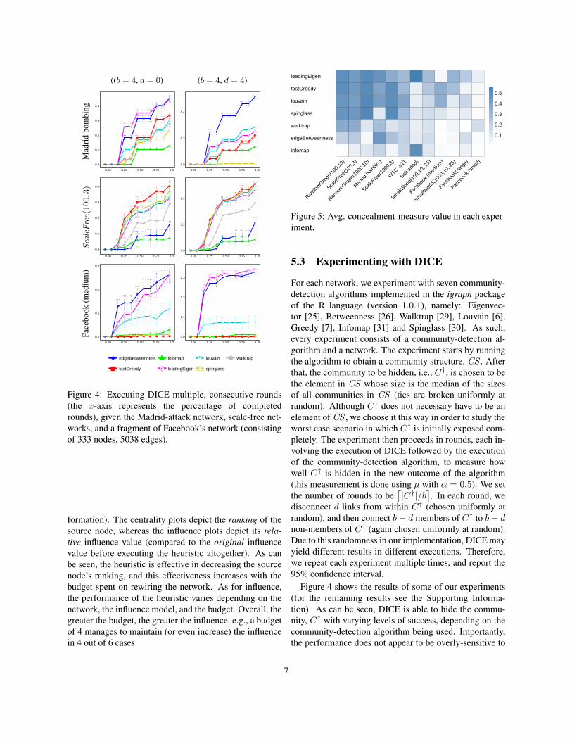
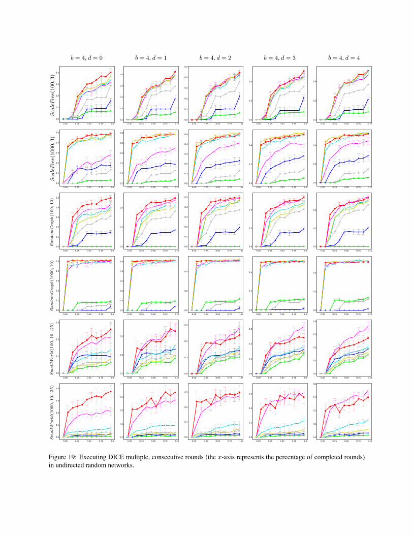
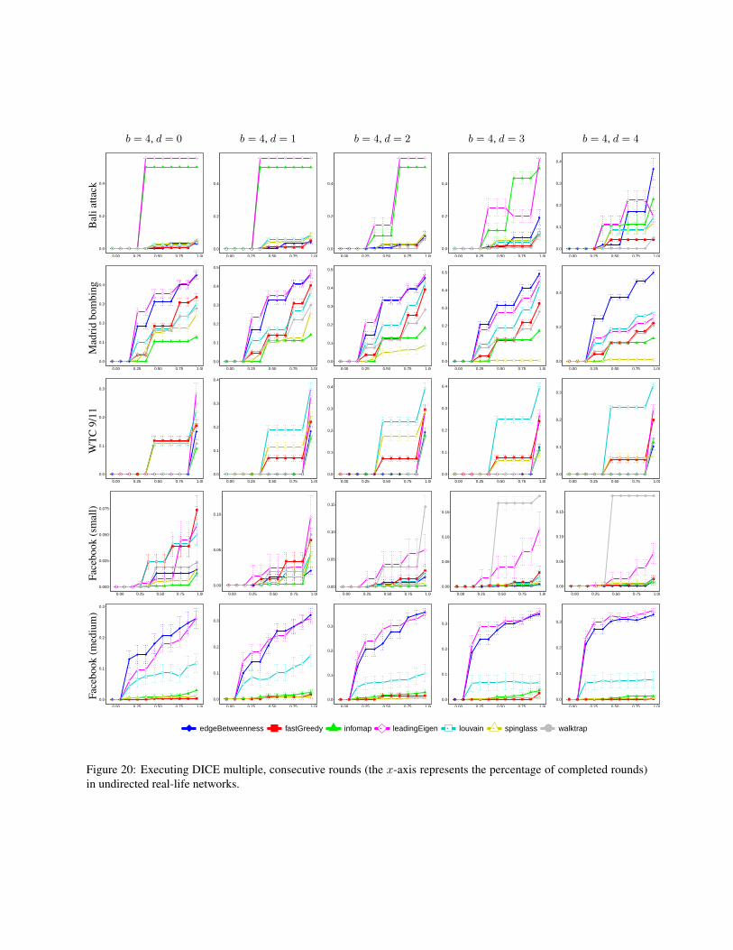
Figure 4: Executing DICE multiple, consecutive rounds(the x-axis represents the percentage of completedrounds), given the Madrid-attack network, scale-free net-works, and a fragment of Facebook’s network (consistingof 333 nodes, 5038 edges).

formation). The centrality plots depict the ranking of thesource node, whereas the influence plots depict its rela-tive influence value (compared to the original influencevalue before executing the heuristic altogether). As canbe seen, the heuristic is effective in decreasing the sourcenode’s ranking, and this effectiveness increases with thebudget spent on rewiring the network. As for influence,the performance of the heuristic varies depending on thenetwork, the influence model, and the budget. Overall, thegreater the budget, the greater the influence, e.g., a budgetof 4 manages to maintain (or even increase) the influencein 4 out of 6 cases.

infomap

edgeBetweenness

walktrap

spinglass

louvain

fastGreedy

leadingEigen

Rando

mGra

ph(1

00,1

0)

ScaleF

ree(

100,

3)

Rando

mGra

ph(1

000,

10)

Mad

rid b

ombin

g

ScaleF

ree(

1000

,3)

WTC 9

/11

Bali a

ttack

Small

Wor

ld(10

0,10

,.25)

Face

book

(med

ium)

Small

Wor

ld(10

00,1

0,.2

5)

Face

book

( lar

ge)

Face

book

(sm

all)

0.1

0.2

0.3

0.4

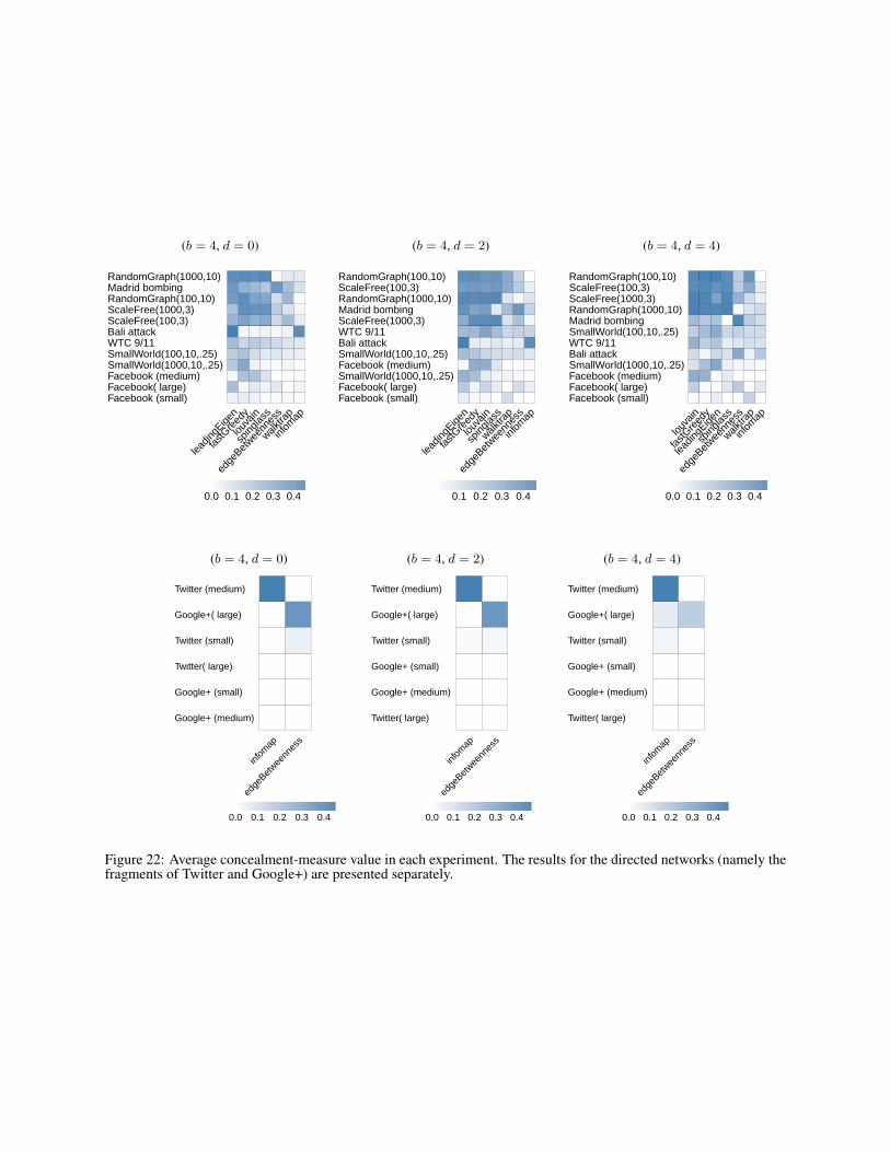
0.5

Figure 5: Avg. concealment-measure value in each exper-iment.

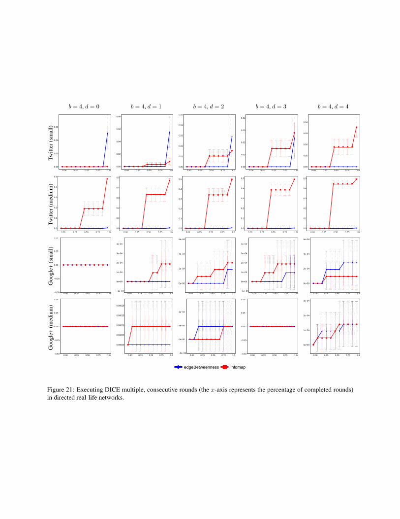
5.3 Experimenting with DICE

For each network, we experiment with seven community-detection algorithms implemented in the igraph packageof the R language (version 1.0.1), namely: Eigenvec-tor [25], Betweenness [26], Walktrap [29], Louvain [6],Greedy [7], Infomap [31] and Spinglass [30]. As such,every experiment consists of a community-detection al-gorithm and a network. The experiment starts by runningthe algorithm to obtain a community structure, CS . Afterthat, the community to be hidden, i.e., C†, is chosen to bethe element in CS whose size is the median of the sizesof all communities in CS (ties are broken uniformly atrandom). Although C† does not necessary have to be anelement of CS , we choose it this way in order to study theworst case scenario in which C† is initially exposed com-pletely. The experiment then proceeds in rounds, each in-volving the execution of DICE followed by the executionof the community-detection algorithm, to measure howwell C† is hidden in the new outcome of the algorithm(this measurement is done using µ with α = 0.5). We setthe number of rounds to be

⌈|C†|/b

⌉. In each round, we

disconnect d links from within C† (chosen uniformly atrandom), and then connect b− d members of C† to b− dnon-members of C† (again chosen uniformly at random).Due to this randomness in our implementation, DICE mayyield different results in different executions. Therefore,we repeat each experiment multiple times, and report the95% confidence interval.

Figure 4 shows the results of some of our experiments(for the remaining results see the Supporting Informa-tion). As can be seen, DICE is able to hide the commu-nity, C† with varying levels of success, depending on thecommunity-detection algorithm being used. Importantly,the performance does not appear to be overly-sensitive to

7

the parameter d. This is important because it provides themembers of C† with the ability to control this parameteras needed (i.e., control the trade-off between the numberof internal edges being removed, and the number of exter-nal edges being added). For example, the members of C†

might be interested in hiding their community as much aspossible, while removing as few internal links as possi-ble (after all, the added external links are fake, serving nopurpose other than disguising the community, whereas theremoved internal links are real; they existed in the com-munity for a reason). In such a case, since the additionof an external link is not entirely under the control of C†

(as it requires the consent of a non-member), the numberof newly-added external links may be insufficient for pro-viding a satisfactory level of concealment, in which casethe members can compensate for this by sacrificing moreinternal links, i.e., by increasing the parameter d.

Figure 5 illustrates the average value of our conceal-ment measure, µ, in each experiment where b = 4 andd = 2. In particular, each row represents a community-detection algorithm, each row represents a network, andthe intensity of the colour in each cell represents the aver-age value of µ, taken over 50 simulations, either by gen-erating a new random network in each simulation, or byre-running the simulation over and over on the same real-life network (recall that our implementation of DICE isnon-deterministic, and may yield different results on thesame network). As can be seen, the Infomap [31] algo-rithm seems to be the most difficult to fool.

6 DiscussionOur goal was to understand the practical limits of disguis-ing individuals and communities, to increase the likeli-hood of them being overlooked by social network anal-ysis tools. Our main result is that, despite the hardnessof finding an optimal solution, disguise is surprisinglyeasy in practice using simple heuristics that are readily-implementable even by lay people. Viewed from a dif-ferent perspective, our work can be seen as an extensionof the sensitivity analyses of centrality measures [8] andcommunity detection algorithms [28]; while such analy-ses typically consider the effects of small network alter-ations, we consider changes that are much wider in scope,and strategic in nature.

On one hand, our findings contribute towards chartingthe limits of protecting privacy in social networks. Onthe other hand, they expose implications for using genericsocial network analysis tools in security applications; thefact that such tools can be easily misled underlines theneed for developing specialized tools that account for the

nature of links and nodes in the network and not just thetopology per se.

Despite these findings, our understanding of how toevade social network analysis tools is still limited, withmany research questions yet to be answered. For in-stance, we still do not know how a relationship can behidden from the eyes of link-prediction algorithms [22],or how an individual can evade detection by Eigenvectorcentrality—the backbone of Google’s search engine.

References[1] European data protection supervisor, meeting the challenges of big

data, opinion 7/2015.

[2] https://govtrequests.facebook.com/.

[3] J. M. Anthonisse. The rush in a graph. Amsterdam: University ofAmsterdam Mathematical Centre, 1971.

[4] A.-L. Barabasi and R. Albert. Emergence of scaling in randomnetworks. science, 286(5439):509–512, 1999.

[5] M. A. Beauchamp. An improved index of centrality. BehavioralScience, 10(2):161–163, 1965.

[6] V. D. Blondel, J.-L. Guillaume, R. Lambiotte, and E. Lefebvre.Fast unfolding of communities in large networks. Journal of Statis-tical Mechanics: Theory and Experiment, 2008(10):P10008, 2008.

[7] A. Clauset, M. E. Newman, and C. Moore. Finding communitystructure in very large networks. Physical review E, 70(6):066111,2004.

[8] C. D. Correa, T. Crnovrsanin, and K.-L. Ma. Visual reasoningabout social networks using centrality sensitivity. Visualizationand Computer Graphics, IEEE Transactions on, 18(1):106–120,2012.

[9] P. Erdos and A. Renyi. On random graphs i. Publ. Math. Debrecen,6:290–297, 1959.

[10] L. C. Freeman. A set of measures of centrality based on between-ness. Sociometry, pages 35–41, 1977.

[11] L. C. Freeman. Centrality in social networks conceptual clarifica-tion. Social networks, 1(3):215–239, 1979.

[12] J. Goldenberg, B. Libai, and E. Muller. Using complex systemsanalysis to advance marketing theory development: Modeling het-erogeneity effects on new product growth through stochastic cel-lular automata. Academy of Marketing Science Review, 9(3):1–18,2001.

[13] B. Hayes. Connecting the dots can the tools of graph theory andsocial-network studies unravel the next big plot? American Scien-tist, 94(5):400–404, 2006.

[14] N. F. Johnson, M. Zheng, Y. Vorobyeva, A. Gabriel, H. Qi, N. Ve-lasquez, P. Manrique, D. Johnson, E. Restrepo, C. Song, andS. Wuchty. New online ecology of adversarial aggregates: Isisand beyond. Science, 352(6292):1459–1463, 2016.

[15] M. Kearns, A. Roth, Z. S. Wu, and G. Yaroslavtsev. Private algo-rithms for the protected in social network search. Proceedings ofthe National Academy of Sciences, page 201510612, 2016.

[16] D. Kempe, J. Kleinberg, and E. Tardos. Maximizing the spreadof influence through a social network. In Proceedings of the ninthACM SIGKDD international conference on Knowledge discoveryand data mining, pages 137–146. ACM, 2003.

8

[17] G. King, J. Pan, and M. E. Roberts. How censorship in chinaallows government criticism but silences collective expression.American Political Science Review, 107(02):326–343, 2013.

[18] G. King, J. Pan, and M. E. Roberts. Reverse-engineering censor-ship in china: Randomized experimentation and participant obser-vation. Science, 345(6199):1251722, 2014.

[19] V. Krebs. Mapping networks of terrorist cells. Connections,24:43–52, 2002.

[20] J. I. Lane, V. Stodden, S. Bender, and H. Nissenbaum, editors. Pri-vacy, big data, and the public good: frameworks for engagement.2014.

[21] J. Leskovec and J. J. Mcauley. Learning to discover social circlesin ego networks. In Advances in neural information processingsystems, pages 539–547, 2012.

[22] L. Lu and T. Zhou. Link prediction in complex networks: A survey.Physica A, 390(6):11501170, 2011.

[23] V. Mayer-Schnberger. Big Data: A Revolution That Will Trans-form How We Live, Work and Think. Viktor Mayer-Schnberger andKenneth Cukier. John Murray Publishers, UK, 2013.

[24] A. Mislove, B. Viswanath, K. P. Gummadi, and P. Druschel. Youare who you know: Inferring user profiles in online social net-works. In Proceedings of the Third ACM International Conferenceon Web Search and Data Mining, WSDM ’10, pages 251–260,New York, NY, USA, 2010. ACM.

[25] M. E. Newman. Finding community structure in networks usingthe eigenvectors of matrices. Physical review E, 74(3):036104,2006.

[26] M. E. Newman and M. Girvan. Finding and evaluating communitystructure in networks. Physical review E, 69(2):026113, 2004.

[27] A. Nordrum. Pro-ISIS Online Groups Use Social Media SurvivalStrategies to Evade Authorities, 2016.

[28] G. K. Orman and V. Labatut. A comparison of community detec-tion algorithms on artificial networks. In Discovery science, pages242–256. Springer, 2009.

[29] P. Pons and M. Latapy. Computing communities in large networksusing random walks. In Computer and Information Sciences-ISCIS2005, pages 284–293. Springer, 2005.

[30] J. Reichardt and S. Bornholdt. Statistical mechanics of communitydetection. Physical Review E, 74(1):016110, 2006.

[31] M. Rosvall, D. Axelsson, and C. T. Bergstrom. The map equa-tion. The European Physical Journal Special Topics, 178(1):13–23, 2010.

[32] M. E. Shaw. Group structure and the behavior of individuals insmall groups. The Journal of Psychology, 38(1):139–149, 1954.

[33] D. J. Watts and S. H. Strogatz. Collective dynamics of small-worldnetworks. nature, 393(6684):440–442, 1998.

[34] J. Xie, S. Kelley, and B. K. Szymanski. Overlapping communitydetection in networks: The state-of-the-art and comparative study.ACM Computing Surveys (csur), 45(4):43, 2013.

9

A Organization of the AppendixIn this document, we formally define the relevant centrality measures and influence models, before defining our op-timization problems (Section B). After that, we present the proofs of our theoretical results (Section C), followed bya discussion of various experimental results (Section D). Finally, we study the problem of constructing a networkfrom scratch, designed for the sole purpose of concealing the identity of the leader while ensuring that it is a highlyinfluential node in the network (Section E).

B DefinitionsBasic Notation: LetG = (V,E) ∈ G denote a network, where V = {v1, . . . , vn} is the set of n nodes andE ⊆ V ×Vis the set of edges. A path is a sequence of distinct nodes, 〈vl, . . . , vk〉, such that every two consecutive nodes areconnected by an edge. The length of a path is considered to be the number of edges in that path. For any pair ofnodes, vi, vj in G, the set of all shortest paths between them is denoted by spG(vi, vj), and the distance betweenthem is denoted by dG(vi, vj), where distance is defined as the length of a shortest path between the two. In caseof an undirected network G we do not discern between edges (vi, vj) and (vj , vi); otherwise the network is said tobe directed. Furthermore, G is said to be connected (strongly connected for directed networks) if there exists a pathbetween every pair of nodes in G.

We denote by NpredG (vi) the set of predecessors of vi in G, that is, Npred

G (vi) = {vj ∈ V : (vj , vi) ∈ E}. Onthe other hand, we denote by N succ

G (vi) the set of successors of vi in G, i.e., N succG (vi) = {vj ∈ V : (vi, vj) ∈ E}.

Finally, we denote by NG(vi) the set of neighbours of vi in G, i.e., NG(vi) = NpredG (vi)∪N succ

G (vi). For the case ofundirected graph, we will assume that NG(vi) = Npred

G (vi) = N succG (vi).

To make the notation more readable, we will often denote two arbitrary nodes by v and w, instead of vi and vj .Moreover, we will often omit the network itself from the notation whenever it is clear from the context, e.g., by writingd(v, w) instead of dG(v, w); this applies not only to the notation presented thus far, but to all notation.

We consider a community structure, CS = {C1, . . . , Ck}, to be a partition of the set of nodes into disjointand exhaustive subsets, or communities.2 Formally, it satisfies the following three conditions: ∀Ci∈CSCi ⊆ V ,⋃Ci∈CS Ci = V , and ∀Ci,Cj∈CSCi ∩ Cj = ∅.

Centrality Measures: Formally, a centrality measure [11] is a function c : G× V → R. The degree centrality [32] isdenoted by cdegr, the closeness centrality [5] is denoted by cclos, and the betweeness centrality [3, 10] is denoted bycbetw. Specifically, given a node vi ∈ V and an undirected network, we have:

cdegr(G, vi) =|NG(vi)|n− 1

cclos(G, vi) =n− 1∑

vj∈V dG(vi, vj)

cbetw(G, vi) =2

(n− 1)(n− 2)

∑vj ,vk∈V \{vi}

|{p ∈ spG(vj , vk) : vi ∈ p}||spG(vj , vk)|

On the other hand, given a directed network, we have:

cdegr(G, vi) =|NG(vi)|2(n− 1)

cclos(G, vi) =1

n− 1

∑vj∈V

1

dG(vi, vj)

2Some works have considered overlapping community structures [34]. However, as common in the literature, we restrict our attention to disjointcommunities.

10

cbetw(G, vi) =1

(n− 1)(n− 2)

∑vj ,vk∈V \{vi}

|{p ∈ spG(vj , vk) : vi ∈ p}||spG(vj , vk)|

+|{p ∈ spG(vk, vj) : vi ∈ p}|

|spG(vk, vj)|

Models of Influence: The propagation of influence through the network is often modeled as follows: when a certainnode is sufficiently influenced by its neighbour(s), it becomes “active”, in which case it starts to influence any “inac-tive” neighbour(s) it may have, and so on. Of course, to initiate this propagation process, a set of nodes needs to beactivated right from the start; this set is called the seed set. Assuming that time moves in discrete rounds, we denote byI(t) ⊆ V the set of nodes that are active at round t, implying that I(1) is the seed set. The way influence propagatesfrom the seed set to the remaining nodes depends on the influence model under consideration. Here, the two mainmodels of influence are:

• Independent Cascade [12]: In this model, every pair of nodes is assigned an activation probability, p : V × V →[0, 1]. Then, in every round, t > 1, every node v ∈ V that became active in round t − 1 activates every inactivesuccessor, w ∈ N succ(v) \ I(t − 1), with probability p(v, w). The process ends when there are no new activenodes, i.e., when I(t) = I(t− 1).

• Linear Threshold [16]: In this model, every node v ∈ V is assigned a threshold value tv which is sampled(according to some probability distribution) from the set {0, . . . , |Npred(v)|}. Then, in every round, t > 1, everyinactive node v becomes active, i.e., becomes a member of I(t), if: |I(t− 1)∩Npred(v)|≥ tv . The process endswhen I(t) = I(t− 1).

In either model, the influence of a node, v, on another, w, is denoted by inf G(v, w) and defined as the probability thatw gets activated given the seed set {v} (we make the common assumption that inf G(v, v) = 0 for all v ∈ V ). Theinfluence of v over the entire network G is then: inf G(v) =

∑w∈V inf G(v, w).

First Objective (Disguising a Node): Roughly speaking, given a source node, v†, and a limited budget, b,specifying the maximum number of edges that are allowed to be added or removed, our goal is to first rewire thenetwork so as to minimize the centrality of v†, and then to further rewire the network so as to “recover” the influenceof v† (in an attempt to compensate for any influence that v† might have lost during the centrality-minimization phase).We consider two variants of the influence-recovery problem; the first focuses on the influence of v† over every singlenode, whereas the second focuses on the influence of v† over the network as a whole. In both cases, only the additionof edges is considered, since the removal of edges can only decrease the influence of v†. Next, we formally define theaforementioned problems.

Definition 1 (Disguising Centrality) This problem is defined by a tuple, (G, v†, b, c, R, A), where G = (V,E) ∈ Gis a network, v† ∈ V is the source node (whose centrality is to be minimized), b ∈ N is a budget specifying themaximum number of edges that can be added or removed, c : G × V → R is a centrality measure, R ⊆ E is a setof edges whose removal is forbidden, A ⊆ (V × V ) \ E is a set of edges whose addition is forbidden. The goal isthen to identify two sets of edges, R∗ ⊆ (E \ R) and A∗ ⊆ (V × V ) \ (E ∪ A), such that: |A∗|+|R∗|≤ b andG∗ = (V, (E ∪A∗) \R∗) is connected (strongly connected if G is directed) and G∗ is in:

argminG′∈{(V,(E∪A)\R):R⊆(E\R),A⊆(V×V )\(E∪A)}

c(G′, v†).

Definition 2 (Individual Influence recovery) This problem is defined by a tuple, (G, v†, inf , A, f), where G =(V,E) ∈ G is a network, v† ∈ V is the source node (whose influence is to be recovered), inf : V × V → R isan influence measure, A ⊆ (V × V ) \ E is a set of edges whose addition is forbidden, and f : V → R specifies theinfluences to be recovered (i.e., for every vi ∈ V we want the influence of v† over vi to be at least f(vi)). The goal isthen to identify a set of edges, A∗, that is in:

argminA⊆(V×V )\(E∪A):∀vi∈V inf (V,E∪A)(v

†,vi)≥f(vi)|A|.

11

Definition 3 (Global Influence recovery) This problem is defined by a tuple, (G, v†, inf , A, φ), whereG = (V,E) ∈G is a network, v† ∈ V is the source node (whose influence is to be recovered), inf : V × V → R is an influencemeasure, A ⊆ (V × V ) \ E is a set of edges whose addition is forbidden, and φ ∈ R is the total influence to berecovered. The goal is then to identify a set of edges, A∗, that is in:

argminA⊆(V×V )\(E∪A):inf (V,E∪A)(v

†)≥φ|A|.

Second Objectives (Disguising a Community): Roughly speaking, given a community to be hidden, C†, and alimited budget, b, specifying the maximum number of edges that are allowed to be added or removed, our goal isto rewire the network so as to hide C†. To this end, we propose a measure of concealment, µ, defined for everycommunity C† ⊆ V and every community structure CS , as follows:3

µ(C†,CS ) = αµ′(C†,CS ) + (1− α)µ′′(C†,CS ),

where α ∈ [0, 1] and:

µ′(C†,CS ) =|{Ci ∈ CS : Ci ∩ C† 6= ∅}|−1

max(|CS |−1, 1)maxCi∈CS (|Ci ∩ C†|)

µ′′(C†,CS ) =∑

Ci∈CS

|Ci \ C†|max(n− |C†|, 1)

.

Note that µ(C†,CS ) ∈ [0, 1] for all C† and CS , with greater values indicating greater levels of concealment of C† inCS . Having presented our concealment measure, we are now ready to formally introduce our problem.

Definition 4 (Disguising a Community) This problem is defined by a tuple, (G,C†, alg , b), where G = (V,E) is anetwork, C† ⊆ V is the community to be hidden, alg is a community-detection algorithm, and b ∈ N is a budgetspecifying the maximum number of edges that can be added or removed. The goal is then to find a set of edges to beadded,A∗ ⊆ (V ×V )\E, and another to be removed,R∗ ⊆ E, such that |A∗|+|R∗|≤ b andG∗ = (V, (E∪A∗)\R∗)is in:

argmaxG′∈{(V,(E∪A)\R) : A⊆(V×V )\E, R⊆E, |A|+|R|≤b}

µ(C†, alg(G′)),

where alg(G) is the community structure returned by the algorithm alg given the network G.

Note that the above optimization problem requires C† to know the exact community-detection algorithm that theadversary is using. Since such knowledge is hardly available, we avoid this requirement, and instead aim to develop ageneral-purpose heuristic, designed for no particular community-detection algorithm.

C Proofs

From the computational point of view, disguising the degree centrality of v† is easy, since the only way to decrease thiscentrality is to remove edges connecting v† to its neighbour(s). Next, we study the problems of disguising closenesscentrality and betweenness centrality, followed by the problem of influence recovery under the Independent-Cascademodel and under the Linear-Threshold model.

Theorem 1 Disguising closeness centrality is NP-complete.

3Note that C† is not necessarily a member of CS . To put it differently, when describing C† as a “community” we use this term in its broadersense, where C† is essentially just a subset of nodes. As such, when measuring how well C† is hidden in CS , it may well be the case that themembers of C† are spread out across multiple communities in CS .

12

Proof. The decision version of the optimization problem is the following: given a network G = (V,E), a source nodev†, two sets R ⊆ E, A ⊆ (V × V ) \ E, a budget b ∈ N and a value x ∈ R, does there exist two sets R∗ ⊆ (E \ R)and A∗ ⊆ (V × V ) \ (E ∪ A) such that |A∗|+|R∗|≤ b, and the network (V, (E ∪ A∗) \ R∗) is connected (stronglyconnected if G is directed) and cclos((V, (E ∪A∗) \R∗), v†) ≤ x?

This problem is in NP, as given a solution, i.e., two sets A∗ and R∗, we can verify whether cclos((V, (E ∪ A∗) \R∗), v†) ≤ x in polynomial time; this only requires computing the closeness centrality of node v† in network (V, (E∪A∗) \R∗).

We will now show that the decision version is NP-hard. To this end, let us denote by q ∈ R the smallest possiblecloseness centrality of v† in any (strongly) connected network whose set of nodes is V . One can see that q = 2/n inthe case of undirected networks, and q = (

∑n−1i=1

1i )/(n− 1) in the case of directed network; this happens if and only

if:

• the network is a path of which v† is an end (when dealing with undirected networks); or

• the network is a directed cycle (when dealing with directed networks).

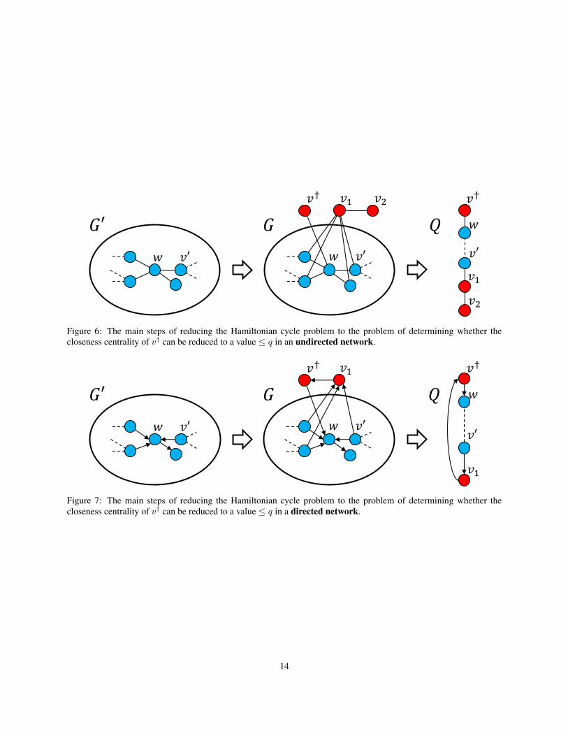
Let us denote such a network by Q; the closeness centrality of v† in Q is then q. With this in mind, the proof involvesa reduction from the Hamiltonian cycle problem (i.e., the problem of determining whether there exists a cycle thatvisits each node exactly once) to the decision problem of determining whether it is possible to reduce the closenesscentrality of v† to a value smaller than, or equal to, q.

To this end, given some arbitrary network, G′ = (V ′, E′), be it directed or undirected, let us modify G′ so as toobtain a new network, G = (V,E), as illustrated in figures 6 and 7. Formally, we do so by choosing some arbitrarynode, w ∈ V ′, and then setting:

V = V ′ ∪ {v†, v1, v2}, E = E′ ∪ {(v†, w), (v1, v2)} ∪ {(v, v1) : v ∈ V ′, v ∈ NG′(w)},

in the case of undirected networks, or setting:

V = V ′ ∪ {v†, v1}, E = E′ ∪ {(v†, w), (v1, v†)} ∪ {(v, v1) : v ∈ V ′, v ∈ NpredG′ (w)},

in the case of directed networks.We will now show that the Hamiltonian cycle problem in G′ is equivalent to the following decision problem: Given

network G and budget b = |E′|−|V ′|+|NpredG′ (w)|, where A = R = ∅, determine whether it is possible to reduce the

closeness centrality of v† to a value≤ q, by removing at most b edges from G. Throughout the remainder of the proof,the edges and nodes in G that were in G′ will be referred to as “original”.

Firstly, we will show that if G′ has a Hamiltonian cycle then it is possible to obtain Q by removing|E′|−|V ′|+|Npred

G′ (w)| edges from G. To this end, fix a Hamiltonian cycle of G′, then:

• remove from G all original edges that are not in the Hamiltonian cycle; there are exactly |E′|−|V ′| such edges;

• in the Hamiltonian cycle, there are exactly two edges of which w is an end; remove any of those edges in theundirected network, or the one pointing to w in the directed network; let us denote the removed edge as (v′, w);

• remove all edges from all predecessors of w to v1, with the exception of (v′, v1); there are exactly |NpredG′ (w)|−1

such edges.

In so doing, we have obtained the network Q by removing a total of |E′|−|V ′|+|NpredG′ (w)| edges from G (see figures

6 and 7).Secondly, we show that if it is possible to obtain Q by removing |E′|−|V ′|+|Npred

G′ (w)| edges from G, then thereexists a Hamiltonian cycle in G′. We will first deal with the undirected case, before moving on to the directed case.

In the undirected case, observe that nodes v† and v2 each have a degree of 1 in G, since their only neighbours are wand v1, respectively. Now since Q is connected, and since we obtained Q by only removing (rather than adding) edgesfrom G, the nodes v† and v2 must each have a degree of 1 in Q. Consequently, they must be the two ends of Q. This,in turn, implies that v1 must have exactly two neighbours in Q; we know that one of them is v2, let us call the other v′.This, as well as the fact that v† is only connected to w, implies that the segment of Q between w and v′ contains all

13

𝑤

𝑣† 𝑣1 𝑣2

𝑣′ 𝑤 𝑣′

𝑣†

𝑣1

𝑣2

𝑤

𝑣′

𝐺′ 𝐺 𝑄

Figure 6: The main steps of reducing the Hamiltonian cycle problem to the problem of determining whether thecloseness centrality of v† can be reduced to a value ≤ q in an undirected network.

𝐺′

𝑣1

𝑣′

𝑣†

𝑤

𝑤

𝑣† 𝑣1

𝑣′ 𝑤 𝑣′

𝑄𝐺

Figure 7: The main steps of reducing the Hamiltonian cycle problem to the problem of determining whether thecloseness centrality of v† can be reduced to a value ≤ q in a directed network.

14

original nodes from G′ and only original edges from G′ (recall that we did not add any edges between original nodes).Finally, by adding to that segment the original edge between v′ and w, we obtain a Hamiltonian cycle in G′.

As for the directed case, we observe that node v† has only one successor in Q, namely w, and only one predecessorinQ, namely v1. We also know that v1 has only one predecessor inQ; let us call that predecessor v′. These facts implythat the segment of Q between w and v′ contains all original nodes from G′ and only original edges from G′ (again,recall that we did not add any edges between original nodes). By adding to that segment the original edge between v′

and w, we obtain a Hamiltonian cycle in G′.We have shown that a Hamiltonian cycle in G′ exists if and only if it is possible to reduce the closeness centrality

of v† to q by removing exactly |E′|−|V ′|+|NpredG′ (w)| edges from G, which concludes the proof. 2

Theorem 2 Disguising betweenness centrality is NP-complete.

Proof. The decision version of the optimization problem is the following: given a network G = (V,E), a source nodev†, two sets R ⊆ E, A ⊆ (V × V ) \ E, a budget b ∈ N and a value x ∈ R, does there exist two sets R∗ ⊆ (E \ R)and A∗ ⊆ (V × V ) \ (E ∪ A) such that |A∗|+|R∗|≤ b, and the network (V, (E ∪ A∗) \ R∗) is connected (stronglyconnected if G is directed) and cbetw((V, (E ∪A∗) \R∗), v†) ≤ x?

This problem is in NP, as given a solution, i.e., two sets A∗ and R∗, we can verify whether cbetw((V, (E ∪ A∗) \R∗), v†) ≤ x in polynomial time; this only requires computing the betweenness centrality of node v† in network(V, (E ∪A∗) \R∗).

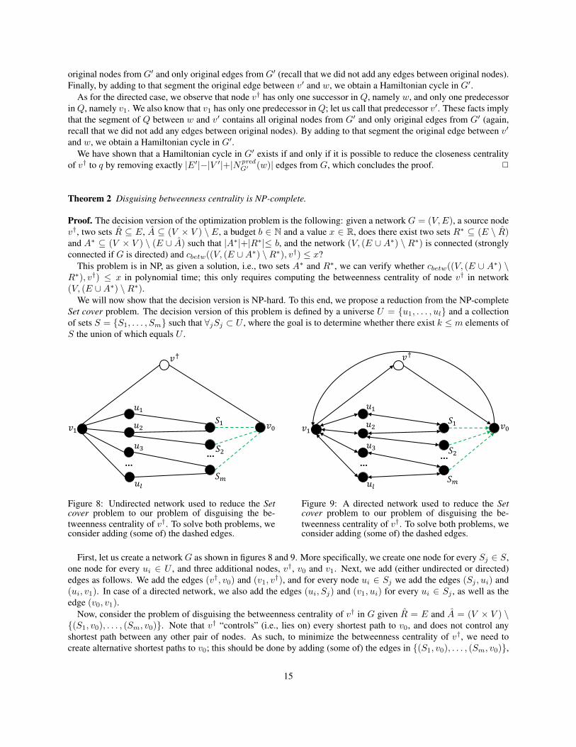
We will now show that the decision version is NP-hard. To this end, we propose a reduction from the NP-completeSet cover problem. The decision version of this problem is defined by a universe U = {u1, . . . , ul} and a collectionof sets S = {S1, . . . , Sm} such that ∀jSj ⊂ U , where the goal is to determine whether there exist k ≤ m elements ofS the union of which equals U .

𝑣1

𝑢1

𝑢2

𝑢3...

𝑆1

𝑆2

𝑆𝑚

𝑣0

𝑢𝑙

...

𝑣†

Figure 8: Undirected network used to reduce the Setcover problem to our problem of disguising the be-tweenness centrality of v†. To solve both problems, weconsider adding (some of) the dashed edges.

......

𝑣1

𝑢1

𝑢2

𝑢3

𝑆1

𝑆2

𝑆𝑚

𝑣0

𝑢𝑙

𝑣†

Figure 9: A directed network used to reduce the Setcover problem to our problem of disguising the be-tweenness centrality of v†. To solve both problems, weconsider adding (some of) the dashed edges.

First, let us create a network G as shown in figures 8 and 9. More specifically, we create one node for every Sj ∈ S,one node for every ui ∈ U , and three additional nodes, v†, v0 and v1. Next, we add (either undirected or directed)edges as follows. We add the edges (v†, v0) and (v1, v

†), and for every node ui ∈ Sj we add the edges (Sj , ui) and(ui, v1). In case of a directed network, we also add the edges (ui, Sj) and (v1, ui) for every ui ∈ Sj , as well as theedge (v0, v1).

Now, consider the problem of disguising the betweenness centrality of v† in G given R = E and A = (V × V ) \{(S1, v0), . . . , (Sm, v0)}. Note that v† “controls” (i.e., lies on) every shortest path to v0, and does not control anyshortest path between any other pair of nodes. As such, to minimize the betweenness centrality of v†, we need tocreate alternative shortest paths to v0; this should be done by adding (some of) the edges in {(S1, v0), . . . , (Sm, v0)},

15

since no other edge can be added, and no edge can be removed (following the definitions of R and A). To be moreprecise, we can add at most b edges {(S1, v0), . . . , (Sm, v0)}, since we cannot exceed the budget. After this process,the betweenness centrality of v† may drop to as little as q = 2

(n−1)(n−2) in the undirected case, or as little as q =1

(n−1)(n−2) in the directed case; this happens when v† no longer controls any of the shortest paths to v0 except for theone from v1 to v0. Note that adding an edge (Sj , v0) creates a new shortest path from every nodes ui ∈ Sj to v0. Thisimplies that the betweenness centrality of v† can be reduced to q if and only if there exists at most b elements of S theunion of which equals U .

We have just reduced the decision version of the Set Cover problem given k to the following decision problem:Given network G and budget b = k, where R = E and A = (V × V ) \ {(S1, v0), . . . , (Sm, v0)}, determine whetherit is possible to reduce the closeness centrality of v† to some value ≤ q, by removing at most b edges from G. 2

Theorem 3 Both the global and the individual influence recovery problems are NP-hard under the Independent Cas-cade model.

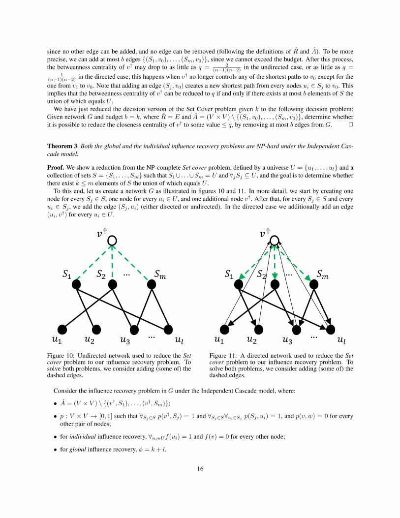
Proof. We show a reduction from the NP-complete Set cover problem, defined by a universe U = {u1, . . . , ul} and acollection of sets S = {S1, . . . , Sm} such that S1∪ . . .∪Sm = U and ∀jSj ⊆ U , and the goal is to determine whetherthere exist k ≤ m elements of S the union of which equals U .

To this end, let us create a network G as illustrated in figures 10 and 11. In more detail, we start by creating onenode for every Sj ∈ S, one node for every ui ∈ U , and one additional node v†. After that, for every Sj ∈ S and everyui ∈ Sj , we add the edge (Sj , ui) (either directed or undirected). In the directed case we additionally add an edge(ui, v

†) for every ui ∈ U .

𝑣†

𝑆1 …

…

𝑆2 𝑆𝑚

𝑢1 𝑢𝑙𝑢2 𝑢3

Figure 10: Undirected network used to reduce the Setcover problem to our influence recovery problem. Tosolve both problems, we consider adding (some of) thedashed edges.

𝑣†

𝑆1 …

…

𝑆2 𝑆𝑚


Figure 11: A directed network used to reduce the Setcover problem to our influence recovery problem. Tosolve both problems, we consider adding (some of) thedashed edges.

Consider the influence recovery problem in G under the Independent Cascade model, where:

• A = (V × V ) \ {(v†, S1), . . . , (v†, Sm)};

• p : V × V → [0, 1] such that ∀Sj∈S p(v†, Sj) = 1 and ∀Sj∈S∀ui∈Sj

p(Sj , ui) = 1, and p(v, w) = 0 for everyother pair of nodes;

• for individual influence recovery, ∀ui∈Uf(ui) = 1 and f(v) = 0 for every other node;

• for global influence recovery, φ = k + l.

16

The goal is then to identify the smallest subset of edges to be added to the network, A ⊆ {(v†, S1), . . . , (v†, Sm)},

such that either inf (V,E∪A)(v†) ≥ φ in the global variant of the problem, or ∀vi∈V inf (V,E∪A)(v

†, vi) ≥ f(vi) in theindividual variant of the problem.

Recall that the influence of v† is measured by setting the seed set as {v†} and calculating the probability that othernodes get activated. Also recall that under the Independent Cascade model an active node, v, activates any of itspredecessors, w, with probability p(v, w). Importantly, with the p function defined as above, adding an edge (v†, Sj)for some Si ∈ S makes the influence of v† on every ui ∈ Sj equal to 1. Furthermore, the above definitions of φand f imply that our goal (in both the individual and the global variants of the problem) is achieved if and only if theinfluence of v† on every node ui ∈ U equals 1. Consequently, our goal is achieved if and only if we add to G a set ofedges, A ⊆ {(v†, S1), . . . , (v

†, Sm)}, such that: ⋃(v†,Sj)∈A

Sj = U.

Since we are interested in finding the smallest such subset, a solution to the above instance of the influence recoveryproblem gives us a solution to the Set Cover problem. 2

Theorem 4 Both the global and the individual influence recovery problems are NP-hard under the Linear Thresholdmodel.

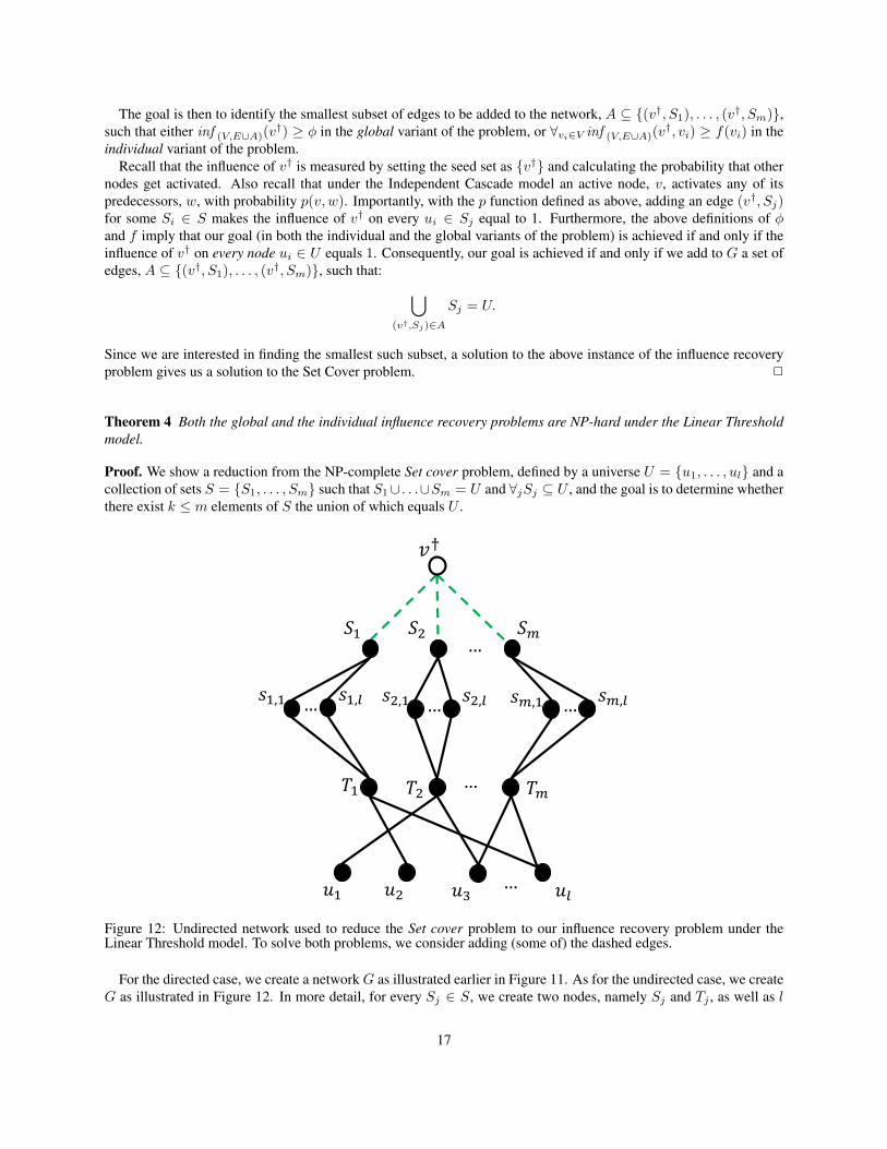
Proof. We show a reduction from the NP-complete Set cover problem, defined by a universe U = {u1, . . . , ul} and acollection of sets S = {S1, . . . , Sm} such that S1∪ . . .∪Sm = U and ∀jSj ⊆ U , and the goal is to determine whetherthere exist k ≤ m elements of S the union of which equals U .

𝑇1 …

…

𝑇2 𝑇𝑚


𝑆1…

𝑆2 𝑆𝑚

…𝑠1,1 𝑠1,𝑙 …

𝑠2,1 𝑠2,𝑙 …𝑠𝑚,1 𝑠𝑚,𝑙

𝑣†

Figure 12: Undirected network used to reduce the Set cover problem to our influence recovery problem under theLinear Threshold model. To solve both problems, we consider adding (some of) the dashed edges.

For the directed case, we create a network G as illustrated earlier in Figure 11. As for the undirected case, we createG as illustrated in Figure 12. In more detail, for every Sj ∈ S, we create two nodes, namely Sj and Tj , as well as l

17

additional nodes, namely sj,1, . . . , sj,l. We also create one node for every ui ∈ U , and finally add the source node, v†.As for the edges, for every Sj ∈ S and every ui ∈ Sj , we add the edge (Tj , ui). Furthermore, for every node sj,i, weadd the edges (Sj , sj,i) and (sj,i, Tj).

Now consider the influence recovery problem in G under the Linear Threshold model, where:

• A = (V × V ) \ {(v†, S1), . . . , (v†, Sm)};

• tv = l for every node v ∈ {T1, . . . , Tm} and tv = 1 for every other node;

• for individual influence recovery, ∀ui∈Uf(ui) = 1 and f(v) = 0 for every other node;

• for global influence recovery, φ = k + l for the directed case, and φ = k(l + 2) + l for the undirected case.

The goal is then to identify the smallest subset of edges to be added to the network, A ⊆ {(v†, S1), . . . , (v†, Sm)},

such that either inf (V,E∪A)(v†) ≥ φ in the global variant of the problem, or ∀vi∈V inf (V,E∪A)(v

†, vi) ≥ f(vi) in theindividual variant of the problem.

Recall that the influence of v† is measured by setting the seed set as {v†} and calculating the probability that othernodes get activated. Also recall that under the Linear Threshold model a node, v, gets activated if the number of itsactive predecessors exceeds tv . Note that, with tv defined as above, adding an edge (v†, Sj) in the undirected caseleads to the activation of nodes si,j and Ti, which in turn leads to the activation of every ui ∈ Sj (see Figure 12).Likewise, in the directed case, adding (v†, Sj) leads to the activation of every ui ∈ Sj (see Figure 11). To put itdifferently, when adding (v†, Sj), the influence of v† on every ui ∈ Sj equals 1. Importantly, the above definitions ofφ and f imply that our goal (in both the individual and the global variants of the problem) is achieved if and only ifthe influence of v† on every node ui ∈ U equals 1. Those observations imply that our goal is achieved if and only ifwe add to G a set of edges, A ⊆ {(v†, S1), . . . , (v

†, Sm)}, such that:⋃(v†,Sj)∈A

Sj = U.

Since we are interested in finding the smallest such subset, a solution to the above instance of the influence recoveryproblem gives us a solution to the Set Cover problem. 2

D Empirical Evaluation

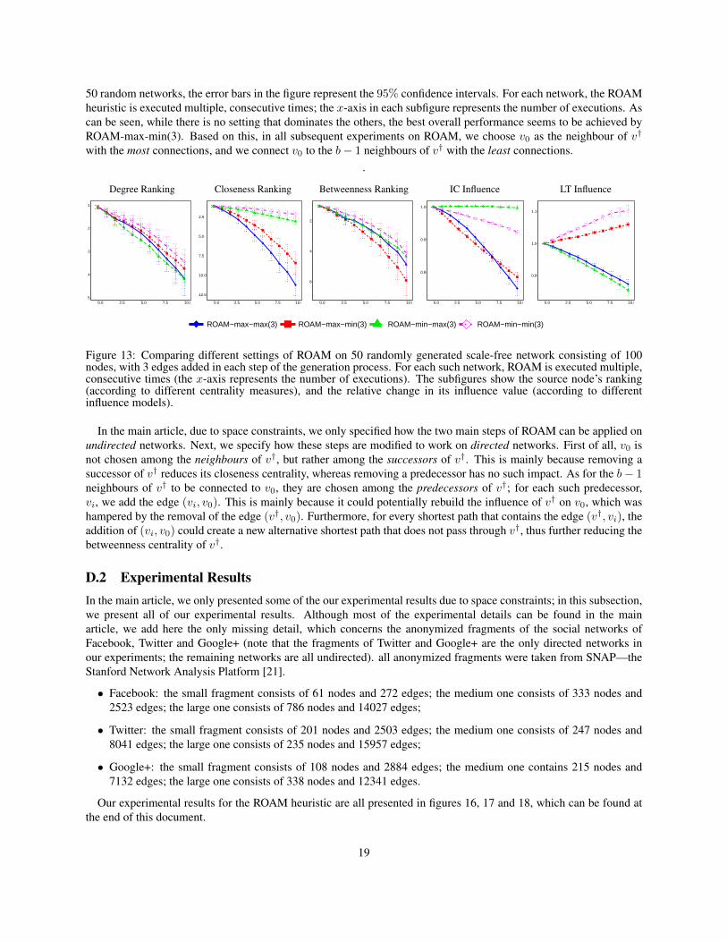
D.1 Configuring the ROAM HeuristicAs mentioned in the main article, the ROAM heuristic involves choosing v0 (the neighbour of v† whom the heuristicwill disconnect from v†), and choosing the b−1 neighbours of v† whom the heuristic will connect to v0. We conducteda number of experiments to determine whether it is more beneficial to choose v0 as the neighbour of v† with the leastconnections or the most connections. Likewise, we wanted to determine whether it is more beneficial to choose theb − 1 neighbours of v† (who will be connected to v0) as the ones with the least connections or the most connections.In particular, Figure 13 compares the different settings given 50 radomly generated scale-free networks consisting of100 nodes each, where 3 edges are added with each step of the generation process (for more details, see [4]); wechose scale-free networks as they resemble real-life networks in many way, e.g., in terms of degree distribution. Asfor the source node, it is chosen to be the one with the lowest sum of centrality rankings (ties are broken uniformly atrandom). As for the Independent Cascade model, we set the activation probability to be p(v, w) = 0.15 for every pairof nodes, v, w ∈ V . As for the Linear Threshold model, for every node, v ∈ V , the threshold value, tv , is sampleduniformly at random from the set {0, . . . , |Npred(v)|}. For both models, the influence values are approximated usingthe Monte-Carlo method. In the figure, we write ROAM-x-y(b), where x can either be “max” or “min” (indicatingthat v0 is the neighbour with the most connections or the least connections, respectively) and y can either be “max” or“min” (indicating that the b−1 neighbours are chosen to be the ones with the most connections or the least connections,respectively), whereas b represents the budget (which is set to 3 in this experiment). Since the results are averaged over

18

50 random networks, the error bars in the figure represent the 95% confidence intervals. For each network, the ROAMheuristic is executed multiple, consecutive times; the x-axis in each subfigure represents the number of executions. Ascan be seen, while there is no setting that dominates the others, the best overall performance seems to be achieved byROAM-max-min(3). Based on this, in all subsequent experiments on ROAM, we choose v0 as the neighbour of v†

with the most connections, and we connect v0 to the b− 1 neighbours of v† with the least connections..

Degree Ranking Closeness Ranking Betweenness Ranking IC Influence LT Influence1

2

3

4

50.0 2.5 5.0 7.5 10.0

2.5

5.0

7.5

10.0

12.5

0.0 2.5 5.0 7.5 10.0

2

4

6

0.0 2.5 5.0 7.5 10.0

0.8

0.9

1.0

0.0 2.5 5.0 7.5 10.0

0.9

1.0

1.1

0.0 2.5 5.0 7.5 10.0

ROAM−max−max(3) ROAM−max−min(3) ROAM−min−max(3) ROAM−min−min(3)

Figure 13: Comparing different settings of ROAM on 50 randomly generated scale-free network consisting of 100nodes, with 3 edges added in each step of the generation process. For each such network, ROAM is executed multiple,consecutive times (the x-axis represents the number of executions). The subfigures show the source node’s ranking(according to different centrality measures), and the relative change in its influence value (according to differentinfluence models).

In the main article, due to space constraints, we only specified how the two main steps of ROAM can be applied onundirected networks. Next, we specify how these steps are modified to work on directed networks. First of all, v0 isnot chosen among the neighbours of v†, but rather among the successors of v†. This is mainly because removing asuccessor of v† reduces its closeness centrality, whereas removing a predecessor has no such impact. As for the b− 1neighbours of v† to be connected to v0, they are chosen among the predecessors of v†; for each such predecessor,vi, we add the edge (vi, v0). This is mainly because it could potentially rebuild the influence of v† on v0, which washampered by the removal of the edge (v†, v0). Furthermore, for every shortest path that contains the edge (v†, vi), theaddition of (vi, v0) could create a new alternative shortest path that does not pass through v†, thus further reducing thebetweenness centrality of v†.

D.2 Experimental ResultsIn the main article, we only presented some of the our experimental results due to space constraints; in this subsection,we present all of our experimental results. Although most of the experimental details can be found in the mainarticle, we add here the only missing detail, which concerns the anonymized fragments of the social networks ofFacebook, Twitter and Google+ (note that the fragments of Twitter and Google+ are the only directed networks inour experiments; the remaining networks are all undirected). all anonymized fragments were taken from SNAP—theStanford Network Analysis Platform [21].

• Facebook: the small fragment consists of 61 nodes and 272 edges; the medium one consists of 333 nodes and2523 edges; the large one consists of 786 nodes and 14027 edges;

• Twitter: the small fragment consists of 201 nodes and 2503 edges; the medium one consists of 247 nodes and8041 edges; the large one consists of 235 nodes and 15957 edges;

• Google+: the small fragment consists of 108 nodes and 2884 edges; the medium one contains 215 nodes and7132 edges; the large one consists of 338 nodes and 12341 edges.

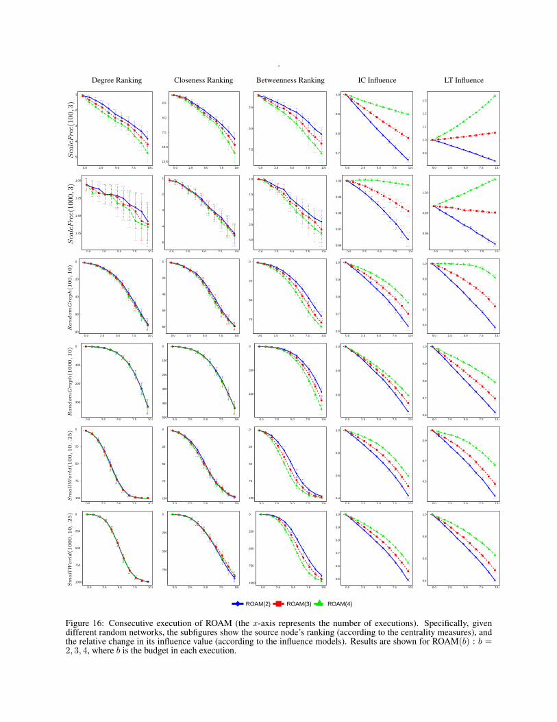
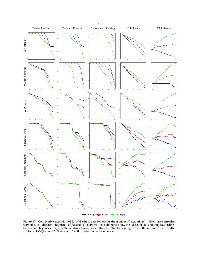
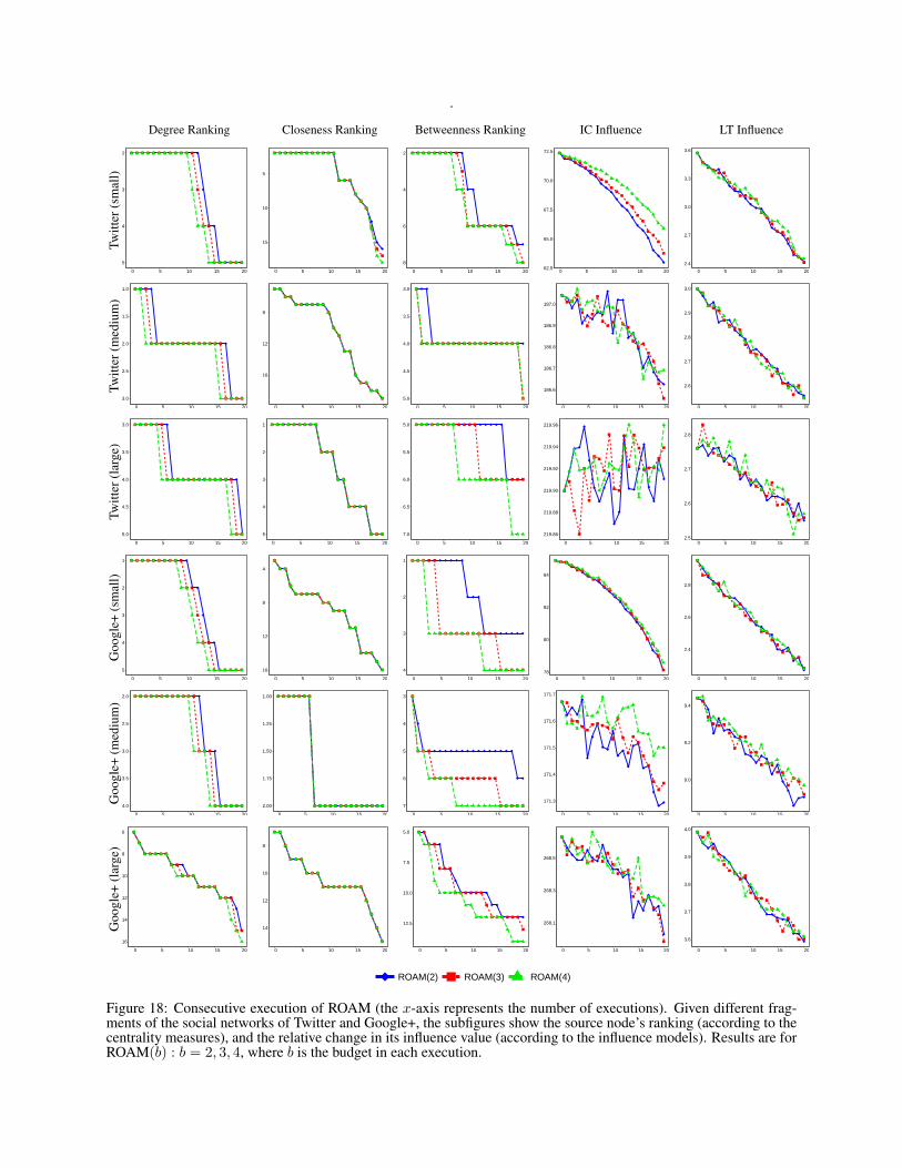
Our experimental results for the ROAM heuristic are all presented in figures 16, 17 and 18, which can be found atthe end of this document.

19

E Constructing a Network from Scratch

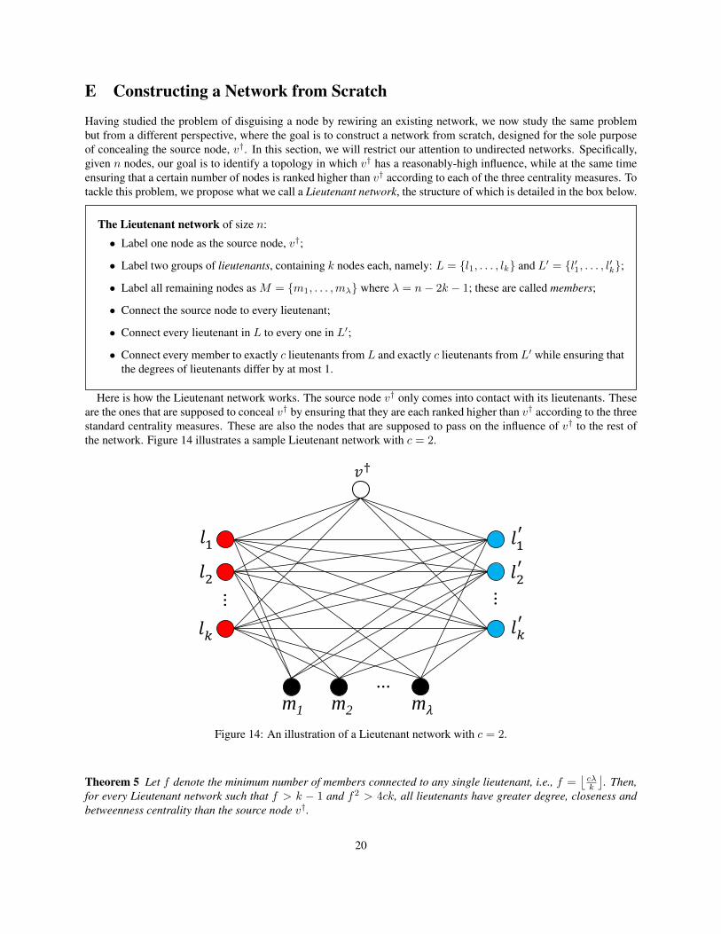
Having studied the problem of disguising a node by rewiring an existing network, we now study the same problembut from a different perspective, where the goal is to construct a network from scratch, designed for the sole purposeof concealing the source node, v†. In this section, we will restrict our attention to undirected networks. Specifically,given n nodes, our goal is to identify a topology in which v† has a reasonably-high influence, while at the same timeensuring that a certain number of nodes is ranked higher than v† according to each of the three centrality measures. Totackle this problem, we propose what we call a Lieutenant network, the structure of which is detailed in the box below.

The Lieutenant network of size n:

• Label one node as the source node, v†;

• Label two groups of lieutenants, containing k nodes each, namely: L = {l1, . . . , lk} and L′ = {l′1, . . . , l′k};

• Label all remaining nodes as M = {m1, . . . ,mλ} where λ = n− 2k − 1; these are called members;

• Connect the source node to every lieutenant;

• Connect every lieutenant in L to every one in L′;

• Connect every member to exactly c lieutenants from L and exactly c lieutenants from L′ while ensuring thatthe degrees of lieutenants differ by at most 1.

Here is how the Lieutenant network works. The source node v† only comes into contact with its lieutenants. Theseare the ones that are supposed to conceal v† by ensuring that they are each ranked higher than v† according to the threestandard centrality measures. These are also the nodes that are supposed to pass on the influence of v† to the rest ofthe network. Figure 14 illustrates a sample Lieutenant network with c = 2.

...

...

m1 m2 m𝜆

...

𝑙1′

𝑙2′

𝑙𝑘′

𝑙1

𝑙2

𝑙𝑘

𝑣†

Figure 14: An illustration of a Lieutenant network with c = 2.

Theorem 5 Let f denote the minimum number of members connected to any single lieutenant, i.e., f =⌊cλk

⌋. Then,

for every Lieutenant network such that f > k − 1 and f2 > 4ck, all lieutenants have greater degree, closeness andbetweenness centrality than the source node v†.

20

Proof. Starting with degree centrality, the degree of the source node, v†, is cdegr(G, v†) = 2kn−1 , since it is only

connected to lieutenants. On the other hand, the degree of a lieutenant, li, is cdegr(G, li) ≥ 1+k+fn−1 , since it is

connected to the source node, to all lieutenants from the other group, and to at least f members. As such, we have:

cdegr(G, li)− cdegr(G, v†) ≥f − k + 1

n− 1

Therefore, cdegr(G, li) > cdegr(G, v†) for all li ∈ L ∪ L′ when f > k − 1.

Moving on to closeness centrality, for any given node, v, this centrality depends inversely on the sum of the lengthsof shortest paths from v to every other nodes, i.e.,

∑u∈V dG(v, u). For both the source node and every lieutenant, the

distance to every other node is either 1 or 2. More precisely, for every v ∈ {v†}∪L∪L′, we have:∑u∈V dG(v, u) =

1|N(v)|+2(n − |N(v)|) = 2n − |N(v)|. Consequently, whenever all lieutenants have greater degree centrality thanv†, they must also have greater closeness centrality than v†. This in turn implies that cclos(G, li) > cclos(G, v

†) forall li ∈ L ∪ L′ when f > k − 1.

Finally, regarding betweenness centrality, let δ(v) denote:∑u,w∈V \{v}:u6=w

|{p∈spG(u,w):v∈p}||spG(u,w)| . Then the between-

ness centrality of a node v ∈ V can be written as: cbetw(G, v) = 2(n−1)(n−2)δ(v). Furthermore, for any two lieu-

tenants, u,w ∈ L ∪ L′ : u 6= w, let γu,w denote the number of members that are neighbours to both of them, i.e.,γu,w = |M ∩NG(u) ∩NG(w)|. Note that, for every pair of lieutenants belonging to the same group, the source nodebelongs to exactly one of the shortest path between those two lieutenants. Based on this, we have:

δ(v†) =∑

u,w∈L:u6=w

1

k + 1 + γu,w+

∑u,w∈L′:u 6=w

1

k + 1 + γu,w

By observing that for any a, b > 0 we have 1a+b <

1a , we conclude that:

δ(v†) <∑

u,w∈L:u6=w

1

k + 1+

∑u,w∈L′:u 6=w

1

k + 1

Now since the number of pairs of different lieutenants from each group is k(k−1)2 < k(k+1)

2 , then:

δ(v†) < k

Having analyzed δ(v†), let us now analyze δ(li) for some lieutenant li ∈ L (the same analysis can be done for alieutenant lj ∈ L′). In particular, since li belongs to shortest paths (i) between every pair of lieutenants from theother group, (ii) between the source node and every member connected to li, and (iii) between every pair of membersconnected to li, we have:

δ(li) =∑

u,w∈L′:u 6=w

1

k + 1 + γu,w+

∑v∈M∩N(li)

1

2c+

∑u,w∈M∩N(li):u 6=w

1

|spG(u,w)|

By omitting the first term of the right-hand side of the equation and observing that |M ∩ N(li)|≥ f and |{{u,w} ⊆M ∩N(li)}|≥ f(f−1)

2 and |spG(u,w)|≤ 2c for every u,w ∈M ∩N(li) : u 6= w, we end up with the following:

δ(li) >f

2c+f(f − 1)

4c>f2

4c

Finally, by comparing δ(v†) with δ(li), we find that:

δ(li)− δ(v†) >f2

4c− k

Therefore, if f2 > 4ck every lieutenant has higher betweenness centrality than the source node. 2

21

As stated in the theorem, a Lieutenant network can indeed conceal its source node as far as centrality is concerned.On the other hand, as far as influence is concerned, we evaluate the network empirically to see how the differentparameters affect the influence of the source node. To this end, given a Lieutenant network of 400 nodes, we variedthe parameters of the network, namely k (the size of each lieutenant group) and c (the number of lieutenants fromeach group, connected to any given member). For every pair, (k, c), we measured the difference in centrality betweenthe source node, v†, and any given lieutenant (the greater the difference, the more v† is disguised), and measured theinfluence of v† to see how this influence is affected by the disguising process.

The results are depicted in Figure 15, where the x-axis represents k and the y-axis represents c.4 Roughly speaking,the results can be categorized into four categories:

• small k and small c: This yields relatively high levels of disguise in terms of betweenness, but not in termsof degree and closeness. On the other hand, it yields rather low levels of Independent-Cascade influence andLinear-Threshold influence;

• small k and large c: This yields relatively high levels of disguise in terms of degree and closeness, but not interms of betweenness. On the other hand, it yields relatively high levels of Independent-Cascade influence, butnot Linear-Threshold influence;

• large k and small c: This yields relatively low levels of disguise in terms of degree, closeness and betweenness.On the other hand, it yields relatively high levels of Linear-Threshold influence, but not Independent-Cascadeinfluence;

• large k and large c: This yields relatively low levels of disguise in terms of degree, closeness and betweenness.On the other hand, it yields relatively high levels of Independent-Cascade influence, but not Linear-Thresholdinfluence.

For future work, it would be interesting to identify other network structures that manage to disguise the source nodeaccording to all three centrality measures, while at the same time maintaining high levels of influence according toboth models of influence.

Degree Closeness Betweenness IC Influence LT Influence

1

2

3

4

5

6

7

8

9

10

10 13 16 19 22 25 28 31 34 37 40

−0.75 −0.50 −0.25 0.00

1

2

3

4

5

6

7

8

9

10

10 13 16 19 22 25 28 31 34 37 40

−0.4 −0.3 −0.2 −0.1 0.0

1

2

3

4

5

6

7

8

9

10

10 13 16 19 22 25 28 31 34 37 40

−0.09 −0.07 −0.05 −0.03

1

2

3

4

5

6

7

8

9

10

10 13 16 19 22 25 28 31 34 37 40

100 200 300

1

2

3

4

5

6

7

8

9

10

10 13 16 19 22 25 28 31 34 37 40

10 20 30 40 50

Figure 15: Given a Lieutenant netowrk of 400 nodes, with different values of parameter k (the x-axis) and parameterc (the y-axis), the figure depicts the difference in centrality between the v† and a lieutenant, as well as the influencevalue of v†.

4we set max(c) ≤ min(k) to ensure that we have a value in every cell of the grid; otherwise some cells would correspond to networks inwhich the are no sufficient lieutenants to connect to.

22

.

Degree Ranking Closeness Ranking Betweenness Ranking IC Influence LT InfluenceScaleFree(100,3

)

1

2

3

4

5

0.0 2.5 5.0 7.5 10.0

2.5

5.0

7.5

10.0

12.5

0.0 2.5 5.0 7.5 10.0

2.5

5.0

7.5

0.0 2.5 5.0 7.5 10.0

0.7

0.8

0.9

1.0

0.0 2.5 5.0 7.5 10.0

0.9

1.0

1.1

1.2

1.3

0.0 2.5 5.0 7.5 10.0

ScaleFree(1000,3

)

1.00

1.25

1.50

1.75

0.0 2.5 5.0 7.5 10.0

1

2

3

4

5

0.0 2.5 5.0 7.5 10.0

1.0

1.5

2.0

2.5

3.0

0.0 2.5 5.0 7.5 10.0

0.96

0.97

0.98

0.99

1.00

0.0 2.5 5.0 7.5 10.0

0.96

0.99

1.02

0.0 2.5 5.0 7.5 10.0

RandomGra

ph(1

00,10)

0

20

40

60

800.0 2.5 5.0 7.5 10.0

0

20

40

60

80

0.0 2.5 5.0 7.5 10.0

0

25

50

75

0.0 2.5 5.0 7.5 10.0

0.6

0.7

0.8

0.9

1.0

0.0 2.5 5.0 7.5 10.0

0.6

0.7

0.8

0.9

1.0

0.0 2.5 5.0 7.5 10.0

RandomGra

ph(1

000,10) 0

100

200

300

0.0 2.5 5.0 7.5 10.0

0

100

200

300

400

5000.0 2.5 5.0 7.5 10.0

0

200

400

0.0 2.5 5.0 7.5 10.0

0.8

0.9

1.0

0.0 2.5 5.0 7.5 10.0

0.6

0.7

0.8

0.9

1.0

0.0 2.5 5.0 7.5 10.0

SmallW

orld

(100,10,.25)

0

25

50

75

100

0.0 2.5 5.0 7.5 10.0

0

25

50

75

100

0.0 2.5 5.0 7.5 10.0

0

25

50

75

100

0.0 2.5 5.0 7.5 10.0

0.4

0.6

0.8

1.0

0.0 2.5 5.0 7.5 10.0

0.5

0.7

0.9

0.0 2.5 5.0 7.5 10.0

SmallW

orld

(1000,10,.25) 0

250

500

750

1000

0.0 2.5 5.0 7.5 10.0

0

250

500

750

0.0 2.5 5.0 7.5 10.0

0

250

500

750

1000

0.0 2.5 5.0 7.5 10.0

0.5

0.6

0.7

0.8

0.9

1.0

0.0 2.5 5.0 7.5 10.0

0.4

0.6

0.8

1.0

0.0 2.5 5.0 7.5 10.0


Figure 16: Consecutive execution of ROAM (the x-axis represents the number of executions). Specifically, givendifferent random networks, the subfigures show the source node’s ranking (according to the centrality measures), andthe relative change in its influence value (according to the influence models). Results are shown for ROAM(b) : b =2, 3, 4, where b is the budget in each execution.

.

Degree Ranking Closeness Ranking Betweenness Ranking IC Influence LT InfluenceB

alia

ttack

4

8

12

16

0 2 4 6 8

4

8

12

16

0 2 4 6 8

2

4

6

0 2 4 6 8

1.5

2.0

2.5

0 2 4 6 8

6

7

8

9

0 2 4 6 8

Mad

rid

bom

bing

0

5

10

15

20

0 2 4 6 8

5

10

0 2 4 6 8

0

10

20

30

40

0 2 4 6 8

0.6

0.9

1.2

1.5

0 2 4 6 8

10

15

20

0 2 4 6 8

WT

C9/

11 5

10

0 1 2 3 4

4

8

12

0 1 2 3 4

0

5

10

15

20

0 1 2 3 4

0.8

1.0

1.2

0 1 2 3 4

6

7

8

9

0 1 2 3 4

Face

book

(sm

all)

0

10

20

30

0 5 10 15 20

10

20

30

0 5 10 15 20

10

20

30

0 5 10 15 204

6

8

10

0 5 10 15 20

10.0

12.5

15.0

17.5

0 5 10 15 20

Face

book

(med

ium

)

8

12

16

0 5 10 15 20

10

20

30

0 5 10 15 20

10

15

20

25

0 5 10 15 20

137

138

139

140

0 5 10 15 20

30

33

36

39

0 5 10 15 20

Face

book

(lar

ge) 20

30

40

50

60

0 5 10 15 20

0

20

40

60

0 5 10 15 20

0

25

50

75

1000 5 10 15 20

599

600

601

0 5 10 15 20

40.0

42.5

45.0

0 5 10 15 20


Figure 17: Consecutive execution of ROAM (the x-axis represents the number of executions). Given three terroristnetworks, and different fragments of Facebook’s network, the subfigures show the source node’s ranking (accordingto the centrality measures), and the relative change in its influence value (according to the influence models). Resultsare for ROAM(b) : b = 2, 3, 4, where b is the budget in each execution.

.

Degree Ranking Closeness Ranking Betweenness Ranking IC Influence LT InfluenceTw

itter

(sm

all)

2

3

4

5

0 5 10 15 20

5

10

15

0 5 10 15 20

2

4

6

8

0 5 10 15 2062.5

65.0

67.5

70.0

72.5

0 5 10 15 20

2.4

2.7

3.0

3.3

3.6

0 5 10 15 20

Twitt

er(m

ediu

m)

1.0

1.5

2.0

2.5

3.0

0 5 10 15 20

8

12

16

0 5 10 15 20

3.0

3.5

4.0

4.5

5.0

0 5 10 15 20

186.6

186.7

186.8

186.9

187.0

0 5 10 15 20

2.6

2.7

2.8

2.9

3.0

0 5 10 15 20

Twitt

er(l

arge

)

3.0

3.5

4.0

4.5

5.0

0 5 10 15 20

1

2

3

4

5

0 5 10 15 20

5.0

5.5

6.0

6.5

7.0

0 5 10 15 20

219.86

219.88

219.90

219.92

219.94

219.96

0 5 10 15 202.5

2.6

2.7

2.8

0 5 10 15 20

Goo

gle+

(sm

all)

1

2

3

4

5

0 5 10 15 20

4

8

12

16

0 5 10 15 20

1

2

3

4

0 5 10 15 2078

80

82

84

0 5 10 15 20

2.4

2.6

2.8

0 5 10 15 20

Goo

gle+

(med

ium

)

2.0

2.5

3.0

3.5

4.0

0 5 10 15 20

1.00

1.25

1.50

1.75

2.00

0 5 10 15 20

3

4

5

6

7

0 5 10 15 20

171.3

171.4

171.5

171.6

171.7

0 5 10 15 20

9.0

9.2

9.4

0 5 10 15 20

Goo

gle+

(lar

ge)

6

8

10

12

14

16

0 5 10 15 20

8

10

12

14

0 5 10 15 20

5.0

7.5

10.0

12.5

0 5 10 15 20

268.1

268.3

268.5

0 5 10 15 20

3.6

3.7

3.8

3.9

4.0

0 5 10 15 20


Figure 18: Consecutive execution of ROAM (the x-axis represents the number of executions). Given different frag-ments of the social networks of Twitter and Google+, the subfigures show the source node’s ranking (according to thecentrality measures), and the relative change in its influence value (according to the influence models). Results are forROAM(b) : b = 2, 3, 4, where b is the budget in each execution.

b = 4, d = 0 b = 4, d = 1 b = 4, d = 2 b = 4, d = 3 b = 4, d = 4ScaleFree(100,3

)

●

● ●

●●●

●

●●

●

●

0.0

0.1

0.2

0.3

0.4

0.00 0.25 0.50 0.75 1.00

●

●

●

●

●

●● ●

●

●

●

0.0

0.1

0.2

0.3

0.4

0.00 0.25 0.50 0.75 1.00

●●

● ●

●

●

●●

●

●

●

0.0

0.1

0.2

0.3

0.4

0.5

0.00 0.25 0.50 0.75 1.00

●

●●

●●

●

●●●

●

●

0.0

0.2

0.4

0.00 0.25 0.50 0.75 1.00

●

●

●●

●

●

●

●●

● ●

0.0

0.2

0.4

0.00 0.25 0.50 0.75 1.00

ScaleFree(1000,3

)

●

●

●●

●

●●●

●●

●

0.0

0.1

0.2

0.3

0.4

0.5

0.00 0.25 0.50 0.75 1.00

●●

●

●

●● ●

●●

●

●

0.0

0.1

0.2

0.3

0.4

0.5

0.00 0.25 0.50 0.75 1.00

● ●

●

●●

●

● ●

● ●

●0.0

0.1

0.2

0.3

0.4

0.5

0.00 0.25 0.50 0.75 1.00

●●

●

●

●

●●

●

● ●

●

0.0

0.2

0.4

0.00 0.25 0.50 0.75 1.00

●

●● ●

●

●

●● ●

●

●

0.0

0.2

0.4

0.00 0.25 0.50 0.75 1.00

RandomGra

ph(1

00,10)

●

●

●

●

●

●

●

●

●

● ●0.0

0.1

0.2

0.3

0.4

0.5

0.00 0.25 0.50 0.75 1.00

●

●

●●

●

●

●

●●

●

●

0.0

0.2

0.4

0.00 0.25 0.50 0.75 1.00

●

●

●●●

●

●

●●

●●

0.0

0.1

0.2

0.3

0.4

0.5

0.00 0.25 0.50 0.75 1.00

●

●

●

●

● ●

●

●

●

●

●

0.0

0.2

0.4

0.00 0.25 0.50 0.75 1.00

●

●

●●

●

● ●

●

●

●

●

0.0

0.2

0.4

0.00 0.25 0.50 0.75 1.00

RandomGra

ph(1

000,10)

●●●

●●●● ●

●

●

●

0.0

0.1

0.2

0.3

0.4

0.5

0.00 0.25 0.50 0.75 1.00

● ●

●

●

●

●●

●● ●

●

0.0

0.1

0.2

0.3

0.4

0.5

0.00 0.25 0.50 0.75 1.00

●●

●

● ●●

● ● ● ●

●

0.0

0.2

0.4

0.00 0.25 0.50 0.75 1.00

●

●

●

●● ●

● ●

●

●

●0.0

0.2

0.4

0.00 0.25 0.50 0.75 1.00

●● ●

●

●

●● ● ●

●

●0.0

0.2

0.4

0.00 0.25 0.50 0.75 1.00

SmallW

orld

(100,10,.25)

●

● ●●

●

●

● ●

● ●●

0.0

0.1

0.2

0.3

0.00 0.25 0.50 0.75 1.00

●●

●●

●●

●

●

●●●

0.0

0.1

0.2

0.00 0.25 0.50 0.75 1.00

●

●

●

●

●●

●●

●●

●

0.0

0.1

0.2

0.3

0.00 0.25 0.50 0.75 1.00

●

●●

●

●

●

●●

●●

●

0.0

0.1

0.2

0.3

0.00 0.25 0.50 0.75 1.00

●

●

●●

● ●

●

●

● ● ●

0.0

0.1

0.2

0.3

0.4

0.00 0.25 0.50 0.75 1.00

SmallW

orld

(1000,10,.25)

●●

●

● ●●

●● ● ●

●

0.0

0.1

0.2

0.3

0.4

0.00 0.25 0.50 0.75 1.00

●● ●● ●●●

●

● ●

●

0.0

0.1

0.2

0.3

0.4

0.00 0.25 0.50 0.75 1.00

● ●●

● ● ● ●

● ●

● ●

0.0

0.1

0.2

0.3

0.00 0.25 0.50 0.75 1.00

●●●●

●●

●●

● ●●

0.0

0.1

0.2

0.3

0.00 0.25 0.50 0.75 1.00

●● ● ●

●●●●

●●●

0.0

0.1

0.2

0.3

0.4

0.00 0.25 0.50 0.75 1.00

Figure 19: Executing DICE multiple, consecutive rounds (the x-axis represents the percentage of completed rounds)in undirected random networks.

b = 4, d = 0 b = 4, d = 1 b = 4, d = 2 b = 4, d = 3 b = 4, d = 4

Bal

iatta

ck

●●● ● ● ●

● ●

●

●●0.0

0.2

0.4

0.00 0.25 0.50 0.75 1.00

●● ●●●●● ●●

●

●0.0

0.2

0.4

0.00 0.25 0.50 0.75 1.00

●●● ● ●●● ●● ●

●

0.0

0.2

0.4

0.00 0.25 0.50 0.75 1.00

●

●

● ● ●● ● ● ● ●●0.0

0.2

0.4

0.00 0.25 0.50 0.75 1.00

● ● ●

●

● ●● ● ●● ●0.0

0.1

0.2

0.3

0.4

0.00 0.25 0.50 0.75 1.00

Mad

rid

bom

bing

●

●

●●

●● ●

●

●

●

●

0.0

0.1

0.2

0.3

0.4

0.00 0.25 0.50 0.75 1.00

●

●

●

● ● ●

● ● ●

●●

0.0

0.1

0.2

0.3

0.4

0.5

0.00 0.25 0.50 0.75 1.00

●

●

●

●

●● ●

● ●

●

●

0.0

0.1

0.2

0.3

0.4

0.5

0.00 0.25 0.50 0.75 1.00

● ●

●● ●

●

●

●●

●

●

0.0

0.1

0.2

0.3

0.4

0.5

0.00 0.25 0.50 0.75 1.00

● ●

●

●

●●●

●

●●●0.0

0.2

0.4

0.00 0.25 0.50 0.75 1.00

WT

C9/

11

●

● ●● ● ●● ●● ●●0.0

0.1

0.2

0.3

0.00 0.25 0.50 0.75 1.00

●● ●

●

● ●● ● ●● ●0.0

0.1

0.2

0.3

0.4

0.00 0.25 0.50 0.75 1.00

●●●

●

●●●●●●●0.0

0.1

0.2

0.3

0.4

0.00 0.25 0.50 0.75 1.00

●

● ●●● ●●● ●● ●0.0

0.1

0.2

0.3

0.4

0.00 0.25 0.50 0.75 1.00

●●● ● ●● ● ●●

●

●0.0

0.1

0.2

0.3

0.00 0.25 0.50 0.75 1.00

Face

book

(sm

all)

● ●

●

●

●●

● ●●

●

●0.000

0.025

0.050

0.075

0.00 0.25 0.50 0.75 1.00

●

●

●

●●●

●●

●

● ●

0.00

0.05

0.10

0.00 0.25 0.50 0.75 1.00

●

●

●●

● ●●

● ●

●

●

0.00

0.05

0.10

0.15

0.00 0.25 0.50 0.75 1.00

● ● ● ●

● ● ●

●

●

● ●

0.00

0.05

0.10

0.15

0.00 0.25 0.50 0.75 1.00

●

●● ●

●● ●●

●● ●

0.00

0.05

0.10

0.15

0.00 0.25 0.50 0.75 1.00

Face

book

(med

ium

)

0.0

0.1

0.2

0.3

0.00 0.25 0.50 0.75 1.00

0.0

0.1

0.2

0.3

0.00 0.25 0.50 0.75 1.00

0.0

0.1

0.2

0.3

0.00 0.25 0.50 0.75 1.00

0.0

0.1

0.2

0.3

0.00 0.25 0.50 0.75 1.00

0.0

0.1

0.2

0.3

0.00 0.25 0.50 0.75 1.00

●edgeBetweenness fastGreedy infomap leadingEigen louvain spinglass walktrap

Figure 20: Executing DICE multiple, consecutive rounds (the x-axis represents the percentage of completed rounds)in undirected real-life networks.

b = 4, d = 0 b = 4, d = 1 b = 4, d = 2 b = 4, d = 3 b = 4, d = 4

Twitt

er(s

mal

l)

0.00

0.02

0.04

0.06

0.00 0.25 0.50 0.75 1.00

0.00

0.02

0.04

0.06

0.08

0.00 0.25 0.50 0.75 1.00

0.00

0.01

0.02

0.03

0.04

0.05

0.00 0.25 0.50 0.75 1.00

0.00

0.01

0.02

0.03

0.04

0.00 0.25 0.50 0.75 1.00

0.00

0.01

0.02

0.03

0.04

0.00 0.25 0.50 0.75 1.00

Twitt

er(m

ediu

m)

0.0

0.1

0.2

0.3

0.4

0.5

0.00 0.25 0.50 0.75 1.00

0.0

0.1

0.2

0.3

0.4

0.5

0.00 0.25 0.50 0.75 1.00

0.0

0.1

0.2

0.3

0.4

0.5

0.00 0.25 0.50 0.75 1.00

0.0

0.1

0.2

0.3

0.4

0.5

0.00 0.25 0.50 0.75 1.00

0.0

0.1

0.2

0.3

0.4

0.5

0.00 0.25 0.50 0.75 1.00

Goo

gle+

(sm

all)

−0.50

−0.25

0.00

0.25

0.50

0.00 0.25 0.50 0.75 1.00−1e−04

0e+00

1e−04

2e−04

3e−04

4e−04

0.00 0.25 0.50 0.75 1.00

0e+00

2e−04

4e−04

6e−04

0.00 0.25 0.50 0.75 1.00−1e−04

0e+00

1e−04

2e−04

3e−04

4e−04

0.00 0.25 0.50 0.75 1.00

0e+00

2e−04

4e−04

6e−04

0.00 0.25 0.50 0.75 1.00

Goo

gle+

(med

ium

)

−0.50

−0.25

0.00

0.25

0.50

0.00 0.25 0.50 0.75 1.00

0.00000

0.00005

0.00010

0.00015

0.00020

0.00 0.25 0.50 0.75 1.00−5e−05

0e+00

5e−05

1e−04

0.00 0.25 0.50 0.75 1.00−0.50

−0.25

0.00

0.25

0.50

0.00 0.25 0.50 0.75 1.00

0e+00

1e−04

2e−04

3e−04

0.00 0.25 0.50 0.75 1.00

edgeBetweenness infomap

Figure 21: Executing DICE multiple, consecutive rounds (the x-axis represents the percentage of completed rounds)in directed real-life networks.

(b = 4, d = 0) (b = 4, d = 2) (b = 4, d = 4)

Facebook (small)Facebook( large)Facebook (medium)SmallWorld(1000,10,.25)SmallWorld(100,10,.25)WTC 9/11Bali attackScaleFree(100,3)ScaleFree(1000,3)RandomGraph(100,10)Madrid bombingRandomGraph(1000,10)

leadin

gEige

n

fastG

reed

y

louva

in

sping

lass

edge

Betwee

nnes

s

walktra

p

infom

ap

0.0 0.1 0.2 0.3 0.4

Facebook (small)Facebook( large)SmallWorld(1000,10,.25)Facebook (medium)SmallWorld(100,10,.25)Bali attackWTC 9/11ScaleFree(1000,3)Madrid bombingRandomGraph(1000,10)ScaleFree(100,3)RandomGraph(100,10)

leadin

gEige

n

fastG

reed

y

louva

in

sping

lass

walktra

p

edge

Betwee

nnes

s

infom

ap

0.1 0.2 0.3 0.4

Facebook (small)Facebook( large)Facebook (medium)SmallWorld(1000,10,.25)Bali attackWTC 9/11SmallWorld(100,10,.25)Madrid bombingRandomGraph(1000,10)ScaleFree(1000,3)ScaleFree(100,3)RandomGraph(100,10)

louva

in

fastG

reed

y

leadin

gEige

n

sping

lass

edge

Betwee

nnes

s

walktra

p

infom

ap

0.0 0.1 0.2 0.3 0.4

(b = 4, d = 0) (b = 4, d = 2) (b = 4, d = 4)

Google+ (medium)

Google+ (small)

Twitter( large)

Twitter (small)

Google+( large)

Twitter (medium)

infom

ap

edge

Betwee

nnes

s

0.0 0.1 0.2 0.3 0.4

Twitter( large)

Google+ (medium)

Google+ (small)

Twitter (small)

Google+( large)

Twitter (medium)

infom

ap

edge

Betwee

nnes

s

0.0 0.1 0.2 0.3 0.4

Twitter( large)

Google+ (medium)

Google+ (small)

Twitter (small)

Google+( large)

Twitter (medium)

infom

ap

edge

Betwee

nnes

s

0.0 0.1 0.2 0.3 0.4

Figure 22: Average concealment-measure value in each experiment. The results for the directed networks (namely thefragments of Twitter and Google+) are presented separately.

Date post:	06-May-2018
Category:	Documents
Upload:	hoangthien
View:	216 times
Download:	1 times

Marcin Waniek Tomasz Michalak Michael Wooldridge address the above question from an individual’s...

Documents