11
Compartmental differential equations models of botnets and epidemic malware Marco Ajelli, Renato Lo Cigno, Alberto Montresor June 2010 Technical Report # DISI-10-011
| Date post: | 22-Jun-2018 |
| Category: |
Documents |
| Upload: | truongtuyen |
| View: | 220 times |
| Download: | 0 times |

Compartmental differential equations models of botnets and
epidemic malware
Marco Ajelli, Renato Lo Cigno, Alberto Montresor
June 2010
Technical Report # DISI-10-011

Compartmental differential equations models of
botnets and epidemic malware
Marco Ajelli
Fondazione Bruno Kessler, Trento, Italy
and DISI, University of Trento, Italy
Email: [email protected]
Renato Lo Cigno, Alberto Montresor
DISI, University of Trento, Italy
Email: {Renato.locigno,alberto.montresor}@disi.unitn.it
Abstract—Botnets, i.e., large systems of controlled agents,have become the most sophisticated and dangerous way ofspreading malware. Their damaging actions can range frommassive dispatching of e-mail spam messages, to denial of serviceattacks, to collection of private and sensitive information. Unlikestandard computer viruses or worms, botnets spread silentlywithout actively operating their damaging activity, and then areactivated in a coordinated way to maximize the “benefit” ofthe malware. In this paper we propose two models based oncompartmental differential equations derived from “standard”models in biological disease spreading. These models offer insightinto the general behavior of botnets, allowing both the optimaltuning of botnets’ characteristics, and possible countermeasuresto prevent them. We analyze, in closed form, some simpleinstances of the models whose parameters have non-ambiguousinterpretation. We conclude the paper by discussing possiblemodel extensions, which can be used to fine-tune the analysis ofspecific epidemic malware in the case that some parameters canbe obtained from actual measurements of the botnet behavior.
I. INTRODUCTION
A botnet is jargon terminology for a collection of infected
end-hosts, called bots, that are under the control of a human
operator known as botmaster. While originally the term was
coined for legitimate purposes, such as the automated man-
agement of IRC channels through distributed scripting, botnets
are now inherently linked to malicious activities. They have
recently been identified as one of the most important threats
to the security of the Internet [6], [18].
Lifecycle of a botnet can be briefly described as fol-
lows [23]. First, the botnet creator sends out a virus, or worm,
that infects unprotected (or under-protected) machines over
the Internet. Several infection strategies exist, mostly borrowed
from other classes of malware (e.g., e-mail viruses). The worm
payload is the bot itself, a malicious application that logs into
a centralized command-and-control server (C&C). Bots may
remain hidden for a long period, waiting for commands from
the C&C. When one of such commands is received, the bot
autonomously perform the malicious actions for which it has
been instructed. Eventually, the bot code may be discovered
and removed, e.g. by an anti-virus software, bringing back the
end-host to a clean state. While installed the bot code can
switch freely between the hidden and the active state.
Example of attacks performed by botnets include sending
of spam and phishing messages [5], click fraud against major
search engines [8], blackmail based on denial-of-service [14],
and identity theft.
To improve their ability to survive, recent botnets have tried
to avoid the centralized point of failure represented by the
C&C in favor of modern peer-to-peer architectures [12]. The
anti-virus community has responded with more sophisticated
mechanisms to detect and disrupt botnets, in an eternal arms
race between good and evil.
We believe that an appropriate modeling of the botnet threat
is a necessary condition to play this “cops and robber” game.
We are interested in modeling two interconnected phases of
the lifecycle of botnet: the creation phase, which include both
the growth and the maintenance of the botnet network, and
the activity phase, when botnets are actually used by their
botmasters for their malicious purposes. We analyze these
phenomena from a theoretical, high-level point of view, and
we simplify the model by considering only the most common
malicious activity: sending spam messages. From now on, the
term ‘spam’ is used as a synonym of maliciousness; in reality,
any malicious actions can fit in this model, from illicitly using
the CPU, to re–distribute illegal material, to scan the local bulk
memory in search of private/sensitive/important information.
Mathematical models have been already proposed to better
understand both the propagation of Internet worms and dis-
semination protocols [2]–[4], [7], [26], [29] and the evaluation
of intervention options in response to the propagation itself
[20], [30]. The aim of this work is to propose the first
mathematical representation of both the botnet growth and the
activity phase, in order to understand what are the conditions
supporting and what are the ones limiting these processes.
In this paper we show that, by changing the proportion
of active bots in the botnet, botmasters are able to build a
botnet also if the worm is not very transmissible, maximize
the amount of damage performed, and generate multiple waves
of malicious activity without the need of creating a new botnet.
From a mathematical point of view, we adopt the classical
differential equation approach used to model biological dis-
eases [1], [9], [27], which allows both closed form theoretical
results and numerical solutions. In fact, biological diseases
and botnets present surprising similarities: both spread using
an infection mechanism based on contact (or communication);
once infected, both may stay inactive for a long period, still
remaining infectious to other members of the population; and
eventually, both can be cured returning to a non-susceptible,
non-infectious, inactive state.
The paper is structured as follows. Section II introduces

the two botnet models discussed in the following. Section III
analyzes the theoretical properties of the two models, and
Section IV provides some insights on the dynamical behavior,
both analytically and experimentally. Section V discusses
related work, while Section VI introduces extensions to these
models that take into account different and more sophisticated
behaviors. Section VII concludes the work.
II. THE MODELS
We take inspiration from years of modeling human dis-
eases and natural epidemic phenomena to build a class of
models that we deem help understanding modern worms
and botnets in particular. We consider two different cases:
the first one assumes that nodes or agents1, after infection
will be recovered, and recovered nodes cannot be infected
anymore, i.e., they are immune forever as if vaccinated. This
scenario corresponds e.g. to a botnet that exploits a single
vulnerability, and this vulnerability is fixed once and for
all. The second one assumes instead that agents can be re-
infected. This latter case is suitable for worms and malware
for which recovery is not definitive. Examples of this behavior
include botnets that mutate during their lifecycle, exploiting
different vulnerabilities at different times (with some attention
in defining the infection rate of different mutations); but it
can be even happen in machines that are re-installed and
become vulnerable again, maybe only for a finite period of
time [24], [25]. Our study is based on compartmental ordinary
differential equations models. Moreover, we assume a finite
population, which can be arbitrarily large, since our models
are scale–invariant with respect to the number of nodes.
A. Botnets Subject to Immunization
We consider four classes of agents.
Class S: susceptible nodes with a positive risk of infection;
Class I: infectious nodes able to infect the susceptibles;
Class V : spamming nodes able to infect the susceptibles and
actively executing their specific malware;
Class R: removed nodes that have been cured (de–infected)
and are immune to the worm.
We call these botnets I-Botnets since the nodes are immunized
against the worm after recovery.
The epidemic flow among these classes is graphically
represented in Figure 1 with the notation we use after the
normalization with respect to the parameter µ and N (see
Table I for the parameters synopsis). It can be described as
follows.
A susceptible can become an infectious node of the botnet
I at the rate b I+VN
, where b is the transmission rate of the
worm (b > 0) and N is the total population (N > 0).
1 We use the terms “node” and “agent” interchangeably, indicating anythingthat may be subject to the infection and become part of the botnet. For instancean agent can be a PC or a single virtual machine. We instead reserve theterms ‘bot’ and ‘bot code’ to the actual infectious malware when we discussexamples.
TABLE IModel variables and parameters
Notation Description
N total population (nodes in the system)µ switching rate between hidden and active
s, S proportion/number of at–risk–of–infection nodesi, I proportion/number of (hidden) infectious nodesv, V proportion/number of infectious and spamming nodesR number of definitely recovered nodesβ, b normalized, absolute worm transmission rateγ, g normalized, absolute (definitive) recovery ratep apportioning coefficient of infected hidden nodesρ rate of temporary recovery
Infectious nodes can start or stop spamming. Since worms
building botnets are normally entirely quiescent, and conse-
quently very hard to detect, if they do not spam, we assume
that only spamming nodes can be detected and removed.
An infectious node can become a spamming node V with
rate µ/(1 − p), where µ > 0 is the speed of the interchange
between classes V and I; a spamming node stops spamming
and go back to the infectious status I with rate µ/p or can be
removed at rate g > 0; p (0¡p¡1) is an apportioning parameter
describing the aggressiveness of the botnet (smaller p means
more aggressive botnets that tend to spam continuously as
p → 0), p is also the fraction of infected nodes in class I .
s
v
i
r
β
γ
1/p1/(1−p)
Fig. 1. Normalized epidemic flow among agents classes for non re-infectingbotnets
The model described above can be formalized with the
following system of differential equations:
S(τ) = −b I(τ)+V (τ)N
S(τ)
I(τ) = b I(τ)+V (τ)N
S(τ) − µ1−p
I(τ) + µpV (τ)
V (τ) = µ1−p
I(τ) −(
µp+ g)
V (τ)
R(τ) = gV (τ)
(1)
a) Normalization: Since we consider a closed population
the relation N = S(τ)+I(τ)+V (τ)+R(τ) ∀τ holds. Thus we
can consider only three differential equations. Moreover, we
can rewrite Equation (1) in an adimensional form, by defining
t := µτ , s := S/N , i := I/N , v := V/N , β := b/µ and
γ := g/µ. Therefore, we have:
s(t) = −β [i(t) + v(t)] s(t)
i(t) = β [i(t) + v(t)] s(t)− 11−p
i(t) + 1pv(t)
v(t) = 11−p
i(t)−(
1p+ γ)
v(t)
(2)
2

as graphically described in Figure 1. For a complete definition
of Equation (2) we have to assign the initial conditions. Here
we assume the following initial conditions:
• s(0) = s0, where 0 < s0 ≤ 1; note that s0 = 0 means
that the population cannot be infected by the worms and
epidemics cannot occur, while s0 = 1 means that the
population is completely susceptible to the worm;
• v(0) = 0, meaning that there are no active spamming
node at the beginning;
• i(0) = ǫ0, where ǫ0 is typically of the order of 10−N ,
and it is anyway included in the range ]0, 1[; note that
i(0) = 0 and v(0) = 0 means that are no infectious agents
in the population; therefore epidemics cannot occur.
b) Remark: Let us note that, if p → 1 or p → 0,
Equation (2) tends to a classical “SI” model, as the one
analyzed in [20], [29]. Moreover we used µ as normalization
factor because the actual rate of transition between i and
v states does not influence the system, since it is only the
proportion time spent in v that makes the botnet ‘apparent’ and
generate spamming. Finally, notice that using an apportioning
coefficient (p) controlling the transition rates between i and vensures that the sum of agent in I and V states remains equal
to the total number of infected nodes, which is coherent with
the fact that switching between spam and no–spam states is
controlled by the botnet itself.
B. Botnets with Re-Infection
In some cases the vaccination of nodes is not feasible, either
because there is no known anti–worm footprint or simply
because infected nodes must be re–installed from scratch
from a CD-ROM and then upgraded to be vaccinated: the
on-line time between installation and vaccination leave them
susceptible [24], [25]. These are R-Botnets since a node can
be Re-infected after recovery.
Indeed, if re-infection is introduced, many interesting addi-
tional parameters can be considered based on the re-infection
model, even without changing the classes of agents. The
simplest model is when agents in class v can either be removed
with rate γ or return susceptible with rate ρ as shown in
Figure 2 only considering the solid transition rates.
A straightforward extension is considering also the possi-
bility of a preventive cure, which would introduce a direct
transition from class s to class r as indicated by the dashed
arrow in Figure 2. Additionally, if one wants to consider worms
which can mutate to make complete recovery more difficult,
one can introduce different infectious rates parameterized on
the class as indicated by the parameter βc in the dashed box in
Figure 2. However, to maintain discussion simple, we will only
consider the fundamental case (without considering dashed
lines ‘extensions’).
Using the same normalization approach we used in Sec-
tion II-A, the model in Figure 2, considering only the solid-
line transitions and and not mutations is formalized by the
s
v
i
rγ
ρ
1/p1/(1−p)
ββc
Fig. 2. Normalized epidemic flow among agents classes for re-infectingbotnets
following set of normalized differential equations:
s(t) = −β [i(t) + v(t)] s(t) + ρv(t)
i(t) = β [i(t) + v(t)] s(t)− 11−p
i(t) + 1pv(t)
v(t) = 11−p
i(t)−(
1p+ ρ+ γ
)
v(t)
(3)
notice that the special case ρ = 0 is the model we discussed
in Section II-A.
C. Plausible Ranges for Transmission and Recovery Rates
Before proceeding with the analysis of the models, we
would like to restrict the meaningful range of the β and γparameters. Let us start with the recovery rate. We normalized
the system with respect to µ, which describes the transition
rate of botnets agents between the spamming and the non-
spamming states. With the assumption that agents in state icannot be detected, we must have γ < 1. In the following we
will always use γ = 0.25, but any other values < 1 can be
used and the fundamental properties of the system will not
change.
Figure 3 reports the maximum fraction of nodes which are
simultaneously infected during the epidemic (plot (A)), and
the fraction of nodes r∞ that have contracted the worm and
recovered at the end of the epidemic itself (plot (B)) as a
function of the ratio β/γ. A quick inspection of the behavior
shows that for β/γ > 10, the fraction of infected nodes tends
to 1 and, for small p, also the fraction of nodes infected at
the same time tends to one. This is a behavior that, to the
best of our knowledge, has not yet been observed in botnets.
Indeed, this also seems to be an unlikely case in modern
Internet, where the diversity of hardware, operating systems
and versions thereof make it difficult to imagine a single
worm that can infect the entire population, even if no known
countermeasures are yet available when it appears. Thus in the
following we will restrict the analysis to values β/γ < 16.
In the following sections we discuss the key theoretical
properties of our models, that will be used to show how a
botnet can be efficiently built and exploited, and, at the same
time, how countermeasures can be taken against botnets, even
in face of very aggressive behaviors.
3

(A)
β γ
max(v
(t)+
i(t)
)
0 5 10 15
00.2
50.5
0.7
51
0.2
0.5
0.8
(B)
β γ
r∞
0 5 10 15
00.2
50.5
0.7
51
0.2
0.5
0.8
Fig. 3. I–Botnets. Plot (A): Maximum value of i(t) + v(t) as a function ofthe fraction β/γ for a fixed value of γ = 0.25. The value of p is reportedin the figure. The initial condition is s(0) = 0.99999, i(0) = 0.00001,v(0) = r(0) = 0. Plot (B): Proportion of recovered agents r(t) at theend of the epidemic as a function of the fraction β/γ for a fixed value ofγ = 0.25. In both a and b the value of p are reported in the figure and theinitial condition is s(0) = 0.99999, i(0) = 0.00001, v(0) = r(0) = 0.
III. THEORETICAL PROPERTIES
In order to understand the dynamics of Equations (2)–(3)
the key parameters are the basic and the effective reproductive
numbers.
In mathematical models for the epidemiology of infectious
diseases (included computer worms, as the cases of system
defined by Equations (2)–(3)), the basic reproductive number
R0 is defined as the threshold parameter which determines if
the introduction of an infected agent can lead to an epidemic
(R0 > 1) or not (R0 < 1). Therefore, if R0 < 1, the
introduction of infectious individuals in the population can not
lead to a major epidemic but only to small clusters of cases;
whereas, if R0 > 1, an epidemic can start with a positive
probability.
The basic reproductive number R0 can essentially be in-
terpreted as the number of new infections generated by an
infectious agent during its entire infectivity period, assuming a
completely susceptible population [1]. Similarly, the effective
reproductive number Re(t) can be defined as the number of
new infections generated by an infectious agent at time t, and
hence defines the sustainability of the infection after time t.Considering botnets, if R0 < 1, then we can assume that
the spam generated is very limited and the game is not worth
the effort, thus a worm whose parameters leads to R0 < 1
can be considered non dangerous. Similarly, when Re(t) < 1,
even if R0 > 1, the epidemic is in decreasing phase, i.e.,
(i(t) + v(t)) < 0, or in other words, the nodes in the botnet
are decreasing, and the worm is being eliminated from the
system.
To compute the reproductive numbers we adopt the next–
generation matrix technique introduced by Diekmann and
Heesterbeek in [9]. In particular, we exploit the same method
described in [19], which is a specific adaptation for models
with multiple infectivity classes with mutual interchanges.
A. Threshold Condition for I-Botnets
Note that Equation (2) admits a continuum of equilib-
ria (called disease–free equilibrium) given by (s⋆, 0, 0) (see
Appendix A). Therefore, let us consider the Jacobian J of
Equation (2) restricted to the infectious classes i and v,
computed at the disease–free equilibrium. It can be written
as
J = T +Σ−D ,
where
T = s⋆(
β β0 0
)
is a matrix whose elements are all real non–negative numbers,
and they correspond to the transmission rates;
Σ =
(
− 11−p
1p
11−p
− 1p
)
is a real matrix with positive off–diagonal elements corre-
sponding to transition between the infectivity classes;
D =
(
0 00 γ
)
is a real non-negative diagonal matrix whose strictly positive
element represents the recovery rate.
Since Σ−D is invertible we can compute
−(Σ−D)−1 =1− p
γ
( 1p+ γ 1
p1
1−p1
1−p
)
and, noticing that all its elements are real and positive, it is
possible to estimate R0 as the dominant eigenvalue of the
next–generation matrix K defined as
K = −T (Σ−D)−1
= s⋆1− p
γ
(
β(
1p+ γ + 1
1−p
)
β(
1p+ 1
1−p
)
0 0
)
.
Since det(K) = 0, it follows that the dominant eigenvalue of
K (namely R0) is
R0 =β
γ
1 + γp(1− p)
ps⋆ (4)
R0 represents the main parameter of the system, in fact if
R0 > 1 epidemic will occur. Otherwise if R0 < 1 epidemic
can not occur.
4
Using similar arguments we obtain a formula for the effec-
tive reproductive number:
Re(t) =β
γ
1 + γp(1− p)
ps(t) . (5)
B. Threshold Condition for R-Botnets
Using the same approach, not repeated here for the sake
of brevity, we compute the basic and effective reproductive
number of Equation (3) for R-Botnets:
R0 =β
γ + ρ
1 + (γ + ρ)p(1− p)
ps⋆ (6)
and
Re(t) =β
γ + ρ
1 + (γ + ρ)p(1− p)
ps(t) . (7)
IV. SYSTEM DYNAMICS
I–Botnets (Equation (2)) show the classical threshold be-
havior, with the threshold parameter given in Equation (4).
If R0 > 1, the shape of the epidemic is the classical one:
susceptibles (s) and removed (r) tend to some real positive
value, while the two infectious classes (i, v) tend to zero (see
Appendix A).
On the other hand, the transition phase strongly depends
on p. In particular, by increasing the value of p, class iis favored and the epidemic peak increases in height and
width (see Fig. 4 (A)). The dynamics of v is instead more
complicated. As shown in Figure 4(B), intermediate values
of p favor the proliferation of v. This means that being
excessively aggressive or not sufficiently aggressive are both
bad strategies.
R–Botnets show the same qualitative behavior of I–Botnets,
but quantitative results are different. Not surprisingly, by fixing
the vale of γ + ρ in Equation (3) at the same value of γ in
Equation (2), the dynamics of both i and v in R–Botnets are
higher than the corresponding for I–Botnets (see Fig. 4).
A. Building the Botnet
I–Botnets can always be built, even if the worms are not
much transmissible (i.e. if β is small). As stated before, an
epidemic occurs (i.e., a botnet can be built) only if R0 > 1.
From Equation (4) we can deduce the conditions under which
R0 > 1 holds:
C1: βγs⋆ > 1;
or
C2: βγs⋆ < 1 and
p <1
2
1−1
βs⋆+
√
(
1−1
βs⋆
)2
+4
γ
. (8)
Therefore, by varying p in (0, 1), Equation 8 can always
be verified and thus the threshold condition can always be
satisfied. In conclusion, independently for the countermeasures
(represented by γ), the botnet can always be built simply by
acting on the aggressivity p of the botnet itself.
In the same way, we can derive the conditions for having
R0 > 1 for R-botnets:
C1: βγ+ρ
s⋆ > 1;
or
C2:β
γ+ρs⋆ < 1 and
p <1
2
1−1
βs⋆+
√
(
1−1
βs⋆
)2
+4
γ + ρ
.
Differently from I–Botnets, for each value of p it is possible
to find a value of ρ which is able to interrupt the creation of
a botnet. Therefore, creation of R–Botnets can be interrupted
by a sufficiently large rate of temporary countermeasures ρ,
a results apparently contraddictory. Fig. 5 shows quantitative
estimation on the value of ρ needed to bring the state of the
system in an under-threshold condition.
B. Maximizing the Damage of Botnets
For both I–Botnets and R–Botnets, the total number of spam
sent by the botnet can be defined as
v∞ := k
∫
∞
0
v(t)dt
for any k > 0 representing the number of spam sent by a bot
in the unit of time. Obviously, v∞ increases as v increases
(because 0 ≤ v(t) < 1 ∀t); therefore, the aim of the botmaster
is to maximize v∞.
The value of v∞ can be controlled by varying p, as sug-
gested by Figure 4(B),(D). Given the difficulty in analytically
obtaining the dependence between v∞ and p, a numerical
evaluation on ddpv∞has been performed.
Given γ, I–Botnets have the potential to reach a maximum
amount of damage vmax. Figure 6 shows how, in order to
reach vmax a value of p can always be found, for each
(reasonable) transmission rate β. Surprisingly, β does not
influence the potential damage a botnet can do, which is
instead controlled only by the countermeasures rate γ, which
turns out to be the only parameter that controls the overall
time (integral value on the botnet existence) that agents spend
in states infective of susceptible. On the ohter hand, not
surprisingly, the higher is the transmission potential of the
worm (β), the larger is the set of p such that the damage is
maximum. In particular, Figure 6 shows that optimal values
of p are around 0.1, corresponding to not very aggressive
botnets; i.e. hidden botnets are much more dangerous than very
aggressive ones. Acting in an extremely covert way (p ≈ 0)
is however not efficient as well.
For R–Botnets, the behavior is slightly more complex than
for I–Botnets. The chance of reaching the maximum damage
vmax depends on the temporary recovery rate (ρ) (as shown
in Figure 7). This proves that the temporary countermeasures
have positive effects on limiting the damage of the botnets.
Obviously, the higher the transmission rate, the less effective
are the countermeasures. Interestingly from Figure 7 we can
5

(A) (B)
t
i
0 100 200 300
0.0
0.2
0.4
0.6
0.8
t
v
0 100 200 300
0.0
00
.05
0.1
00
.15
(C) (D)
t
i
0 100 200 300
0.0
0.2
0.4
0.6
0.8
t
v
0 100 200 300
0.0
00
.09
0.1
8
Fig. 4. I–Botnets: Temporal evolution of class i (A) and v (B). Parameter choices: β = 0.5, γ = 0.25; p = 0.1 (black line), p = 0.2 (dashed black line),p = 0.3 (pointed black line), p = 0.4 (grey line), p = 0.5 (dashed grey line), p = 0.6 (pointed grey line). The initial condition for the entire figure iss(0) = 0.999, i(0) = 0.001, v(0) = r(0) = 0. R–Botnets: Temporal evolution of class i (C) and v (D). Parameter choices and initial condition are thesame of figure (A) and (B) but for γ = 0.125 and ρ = 0.125.
ρ
p
0 2 4 6 8 10
0.0
0.5
1.0
2
1
0.5
0.2
Fig. 5. R–Botnets. Black lines represent the parameters subsets where R0 =1. In the areas below each line R0 > 1. Parameter choices are: s⋆ = 1,γ = 0.25; the value of β is reported in the figure.
deduce that very aggressive botnets are not much efficient, as
observed for the case of I–Botnets.
The maximum value of v∞ that can be produced by the
models depends on γ as suggested by Figure 8. This happens
because γ is related to the time that the agents can potentially
spend in the infectivity classes (v and i) as we already noted.
Moreover, Figure 8 shows how vmax depends on γ and not
on the sum γ+ρ. This proves that temporary countermeasures
have measurable effects on the reduction of the optimal set
of p and can reduce the actual damage done by the botnet as
discussed in Figure 7, but only permanent countermeasures (γ)
p
v∞
0 0.2 0.4 0.6 0.8 1
0
vmax
0.125 0.25 0.5 1 2 4
Fig. 6. I–Botnets. Value of v∞ as a function of p. Parameter choices are:γ = 0.25; the value of β is reported in the figure.
are able to considerably reduce the maximum potential damage
of the botnet. Once more, we note that the transmittability βof the worm does not influence at all the maximum potential
damage of the botnet, but only the range of parameters that
can achieve this maximum.
C. Multiple Waves of Spam Messages
Since the parameter p can be remotely changed by the
botmaster controlling the botnet, we want to investigate the
temporal evolution of I–Botnets under the hypothesis of a non–
constant value of p. In this context, an interesting behavior is
6

(A) (B)
p
v∞
0 0.2 0.4 0.6 0.8 1
0
vmax
0.125 0.25 0.5 1 2 4
p
v∞
0 0.2 0.4 0.6 0.8 1
0
vmax
0.125 0.25 0.5 1 2 4
(C) (D)
p
v∞
0 0.2 0.4 0.6 0.8 1
0
vmax
0.125
0.25 0.5 1 2 4
p
v∞
0 0.2 0.4 0.6 0.8 1
0
vmax
0.125
0.25 0.5 1 2 4
Fig. 7. R–Botnets. Value of v∞ as a function of p. Parameter choices are: γ = 0.25, ρ = 0.125 in (A), ρ = 0.25 in (B), ρ = 0.5 in (C), ρ = 1 in (D);the value of β is reported in the figure.
(A) (B)
p
v∞
0 0.2 0.4 0.6 0.8 1
0
vmax1
vmax2
vmax3
p
v∞
0 0.2 0.4 0.6 0.8 1
0
vmax1
vmax2
vmax3
(C) (D)
p
v∞
0 0.2 0.4 0.6 0.8 1
0
vmax1
vmax2
vmax3
p
v∞
0 0.2 0.4 0.6 0.8 1
0
vmax1
vmax2
vmax3
Fig. 8. R–Botnets. Value of v∞ as a function of p obtained by keeping fixed the quantity γ + ρ. Parameters choices are: γ = 0.2, ρ = 0.05 for black dots;γ = 0.125, ρ = 0.125 for dark grey dots; γ = 0.05, ρ = 0.2 for light grey dots; β = 2 in (A), β = 1 in (B), β = 0.5 in (C), β = 0.25 in (D).
7
the possibility of having multiple waves of spam messages.
As stated in Sec. III, the number of new infections over
time depends on the value of Re(t): in particular if Re(t) > 1the number of new infections increases, while if Re(t) < 1 it
decreases. Equation (5) shows the dependence of Re(t) on p.
Using the same argument of Section IV-A, it follows that, for
every value of s(t), it is possible to choose p in such a way
to have Re(t) > 1. Therefore, at any time the botmaster could
increase p for generating a new wave of messages, without the
need of increasing the transmission rate. In general, increasing
the transmission rate β is very hard, because it depends on the
structure of the population where the worm is spreading and
on the infecting capability of the worm. Therefore, to generate
a new wave of spam in botnets, it is an attractive option to
vary the aggressivity parameter (e.g., by using remote controls)
instead of varying the transmissibility parameter.
Here we show an example of a possible alternative definition
of p which implies a multiple waves pattern of i and v.
We assume that p can be defined by the following piecewise
function:
p :=
{
p1 if v(t) ≤ vp2 otherwise
. (9)
Evaluating the number of nodes in a botnet is very simple,
if the botnet is controlled by a C&C centralized server. But
even modern peer-to-peer botnet can easily estimate the size
of an overlay network [13].
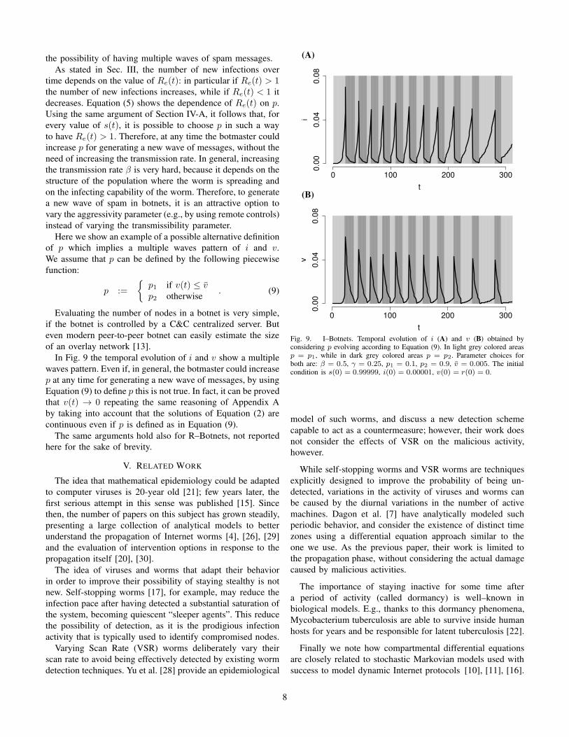
In Fig. 9 the temporal evolution of i and v show a multiple
waves pattern. Even if, in general, the botmaster could increase
p at any time for generating a new wave of messages, by using
Equation (9) to define p this is not true. In fact, it can be proved
that v(t) → 0 repeating the same reasoning of Appendix A
by taking into account that the solutions of Equation (2) are
continuous even if p is defined as in Equation (9).
The same arguments hold also for R–Botnets, not reported
here for the sake of brevity.
V. RELATED WORK
The idea that mathematical epidemiology could be adapted
to computer viruses is 20-year old [21]; few years later, the
first serious attempt in this sense was published [15]. Since
then, the number of papers on this subject has grown steadily,
presenting a large collection of analytical models to better
understand the propagation of Internet worms [4], [26], [29]
and the evaluation of intervention options in response to the
propagation itself [20], [30].
The idea of viruses and worms that adapt their behavior
in order to improve their possibility of staying stealthy is not
new. Self-stopping worms [17], for example, may reduce the
infection pace after having detected a substantial saturation of
the system, becoming quiescent “sleeper agents”. This reduce
the possibility of detection, as it is the prodigious infection
activity that is typically used to identify compromised nodes.
Varying Scan Rate (VSR) worms deliberately vary their
scan rate to avoid being effectively detected by existing worm
detection techniques. Yu et al. [28] provide an epidemiological
(A)
t
i
0 100 200 300
0.0
00
.04
0.0
8
(B)
t
v
0 100 200 3000
.00
0.0
40
.08
Fig. 9. I–Botnets. Temporal evolution of i (A) and v (B) obtained byconsidering p evolving according to Equation (9). In light grey colored areasp = p1, while in dark grey colored areas p = p2. Parameter choices forboth are: β = 0.5, γ = 0.25, p1 = 0.1, p2 = 0.9, v = 0.005. The initialcondition is s(0) = 0.99999, i(0) = 0.00001, v(0) = r(0) = 0.
model of such worms, and discuss a new detection scheme
capable to act as a countermeasure; however, their work does
not consider the effects of VSR on the malicious activity,
however.
While self-stopping worms and VSR worms are techniques
explicitly designed to improve the probability of being un-
detected, variations in the activity of viruses and worms can
be caused by the diurnal variations in the number of active
machines. Dagon et al. [7] have analytically modeled such
periodic behavior, and consider the existence of distinct time
zones using a differential equation approach similar to the
one we use. As the previous paper, their work is limited to
the propagation phase, without considering the actual damage
caused by malicious activities.
The importance of staying inactive for some time after
a period of activity (called dormancy) is well–known in
biological models. E.g., thanks to this dormancy phenomena,
Mycobacterium tuberculosis are able to survive inside human
hosts for years and be responsible for latent tuberculosis [22].
Finally we note how compartmental differential equations
are closely related to stochastic Markovian models used with
success to model dynamic Internet protocols [10], [11], [16].
8

VI. EXTENDING THE MODEL
So far we have only considered the simplest possible models
that capture the property of modern botnet agents of swapping
between active and dormient states without the need of a
centralized control and with apparently random behavior of
single agents.
The technique of compartimental differential equations can
be used of model many other aspects and facets of the botnets
and malware behaviors. We briefly comment on some possible
extensions here.
/(1−q)σ
/(1−q)σ
/qσ
/qσ
s
v
i
rγ
ρ
1/(1−p)
sd id
β
/(1−q)
/q
σ
σ
1/p
vd
Fig. 10. A model for nodes that switch on and off with rate σ
For instance a model like the one represented in Fig. 10 can
represent a system where nodes are not always on line (only
susceptibles and infected dormient are meaningful with this
respect), but they switch on and off with a rate σ and are
on-line with proportion q. Nodes that are switched off while
actually spamming will go into the infective but not spamming
status when switched on again, thus potentially giving an
illusion of problem solution. We set the on-off ratio and rate
equal for all states, but this can be easily modifyied, for
instance to represent users behavior that aggressively switch
node off if they recognize some malicious behavior.
VII. CONCLUSIONS
This work introduced the use of compartmental differential
equations to model the spreading of botnets-creating worms,
as well as, for the first time to the best of our knowledge,
to model the amount of damage (e.g., the number of spam
messages) the botnet can cause during its lifetime.
Results underline how a botnet can be easily built using
worms that are not very transmissible, and how a botnet can
have a great impact in terms of spamming. Moreover, it proves
how a botnet built by a single worm can cause multiple waves
of spamming just by changing the probability with which
single agents swap between active and dormient states.
Thus, this study highlights the necessity to identify all the
infected agents in order to limit the proliferation of the botnets.
In fact, it is not sufficient to recognize only the spamming
agents and removing only them, independently of how well it
is done (namely the value of the recovery rate).
The models we analyzed are on purpose the simplest ones,
that are prone to non-ambiguous interpretation even in the
absence of quantitative data to tune the parameters. Many other
models can be derived form these ones, and one has been
shortly introduced at the end of the paper as example.
Indeed, many other hypotheses should be checked and
other containment/mitigation strategies, more sophisticated
than temporary or definitive recovery, can be introduced. For
instance these models only capture the pool of susceptible
computers, while it might be interesting to model the entire
population, including nodes that are protected by antivirus
software before being infected. All these control options could
be quite easily tested by adapting this mathematical model in
order to take them into account.
Further work includes considering non-homogeneous sys-
tems, for instance considering differences in terms of band-
width among agents. Being this work a purely theoretical
study, it will be interesting to extend this paper by testing
its results on real data set.
REFERENCES
[1] R. M. Anderson and R. M. May. Infectious diseases of humans:
dynamics and control. Oxford, UK: Oxford University Press, 1992.[2] D. Carra, R. Lo Cigno, and E. W. Biersack. Graph Based Analysis of
Mesh Overlay Streaming Systems. IEEE Journal on Selected Areas inCommunications, 25(9):1667–1677, Dec. 2007.
[3] D. Carra, R. Lo Cigno, and E. W. Biersack. Stochastic Graph Processesfor Performance Evaluation of Content Delivery Applications in OverlayNetworks. IEEE Trans. on Parallel and Distributed Systems, 19(2):247–261, feb. 2008.
[4] Z. Chen, L. Gao, and K. Kwiat. Modeling the spread of active worms. InProceedings of the 22nd Annual Joint Conference of the IEEE Computerand Communications Societies (INFOCOM’03), volume 3, pages 1890–1900, 2003.
[5] K. Chiang and L. Lloyd. A Case Study of the Rustock Rootkit andSpam Bot. In Proceedings of First USENIX Workshop on Hot Topics in
Understanding Botnets (HotBots’07), 2007.[6] E. Cooke, F. Jahanian, and D. McPherson. The Zombie Roundup:
Understanding, Detecting, and Disrupting Botnets. In Proceedings ofthe USENIX SRUTI Workshop, 2005.
[7] D. Dagon, C. Zou, and W. Lee. Modeling botnet propagation usingtime zones. In Proceedings of the 13th Annual Network and Distributed
System Security Symposium (NDSS’06), Feb. 2006.[8] N. Daswani and M. Stoppelman. The anatomy of Clickbot.A. In
Proceedings of 1st USENIX Workshop on Hot Topics in Understanding
Botnets (HotBots’07), 2007.[9] O. Diekmann and J. A. P. Heesterbeek. Mathematical epidemiology of
infectious diseases: model building, analysis and interpretation. JohnWiley & Son, 2000.
[10] M. Garetto, R. Lo Cigno, M. Meo, and M. Ajmone Marsan.Closed queueing network models of interacting long-lived TCP flows.IEEE/ACM Trans. on Networking, 12(2):300–311, April 2004.
[11] M. Garetto, R. Lo Cigno, M. Meo, and M. Ajmone Marsan. Modelingshort-lived TCP connections with open multiclass queuing networks.Computer Networks, 44(2):153 – 176, 2004.
[12] J. B. Grizzard, V. Sharma, C. Nunnery, B. B. Kang, and D. Dagon.Peer-to-peer botnets: overview and case study. In Proceedings of
First USENIX Workshop on Hot Topics in Understanding Botnets
(HotBots’07), 2007.[13] M. Jelasity, A. Montresor, and O. Babaoglu. Gossip-based aggregation
in large dynamic networks. ACM Trans. Comput. Syst., 23(1):219–252,Aug. 2005.
[14] S. Kandula, D. Katabi, M. Jacob, and A. W. Berger. Botz-4-Sale: Surviv-ing organized DDoS attacks that mimic flash crowds. In Proceedings of
the 2nd Symposium on Networked Systems Design and Implementation
(NSDI’05), May 2005.[15] J. O. Kephart and S. R. White. Directed-graph epidemiological models
of computer viruses. In Proceedings of the IEEE Symposium on Securityand Privacy, pages 343–359, Los Alamitos, CA, USA, 1991. IEEEComputer Society.
9

[16] R. Lo Cigno and M. Gerla. Modeling window based congestion controlprotocols with many flows. Performance Evaluation, 3637:289 – 306,1999.
[17] J. Ma, G. M. Voelker, and S. Savage. Self-stopping worms. InProceedings of the 2005 ACM Workshop on Rapid Malcode (WORM’05),pages 12–21, New York, NY, USA, 2005. ACM.
[18] B. McCarty. Botnets: Big and Bigger. IEEE Security and Privacy,1:87–90, 2003.
[19] S. Merler, P. Poletti, M. Ajelli, B. Caprile, and P. Manfredi. Coinfectioncan trigger multiple pandemic waves. Journal of Theoretical Biology,254(2):499–507, 2008.
[20] D. Moore, C. Shannon, G. M. Voelker, and S. Savage. InternetQuarantine: Requirements for Containing Self-Propagating Code. InProceedings of the 22nd Annual Joint Conference of the IEEE Computer
and Communications Societies (INFOCOM’03), pages 1901– 1910,2003.
[21] W. H. Murray. The application of epidemiology to computer viruses.Comput. Secur., 7(2):139–145, 1988.
[22] N. M. Parrisha, J. D. Dickb, and W. R. Bishaic. Mechanisms of latencyin Mycobacterium tuberculosis. Trends in Microbiology, 6:107–12,1998.
[23] M. Rajab, J. Zarfoss, F. Monrose, and A. Terzis. A multifaceted approachto understanding the botnet phenomenon. In Proceedings of the 6th ACM
SIGCOMM Conference on Internet Measurement, pages 41–52. ACMNew York, NY, USA, 2006.
[24] SANS Istitute Internet Storm Center. Windows XP: Surviving the firstday, 2003. White paper.
[25] SANS Istitute Internet Storm Center. Windows Vista: First steps, 2007.White paper.
[26] S. Shakkottai and R. Srikant. Peer to Peer Networks for DefenseAgainst Internet Worms. In Proceedings of the 2006 Workshop onInterdisciplinary Systems Approach in Performance Evaluation and
Design of Computer & Communications Sytems, 2006.
[27] H. R. Thieme. Mathematics in population biology. Princeton: PrincetonUniversity Press, 2003.
[28] W. Yu, X. Wang, D. Xuan, and D. Lee. Effective detection of activeworms with varying scan rate. In Proceedings of IEEE International
Conference on Security and Privacy in Communication Networks (Se-cureComm), Baltimore, MD, August, 2006.
[29] C. C. Zou, W. Gong, and D. Towsley. Code Red Worm PropagationModeling and Analysis. In Proceedings of the 9th ACM Conference on
Computer and communications security, pages 138 – 147, 2002.
[30] C. C. Zou, W. Gong, and D. Towsley. Worm propagation modeling andanalysis under dynamic quarantine defense. In Proceedings of the 2003
ACM workshop on Rapid malcode, pages 51–60, 2003.
APPENDIX
In this appendix we prove the basic properties of Equa-
tion (2).
A. Proof of the Stability of Disease Free Equilibrium
Equation (2) admits a continuum of equilibria given by
(s⋆, 0, 0), for all 0 < s⋆ ≤ 12. This continuum of equilibria,
commonly called disease free equilibrium (DFE), is unstable
if R0s⋆ > 1; therefore in this case an epidemic occurs. Other-
wise, if R0s⋆ < 1, the DFE is stable, but not asymptotically
stable, and major epidemics can not occur.
Now, let us prove that the DFE is unstable if R0s⋆ > 1.
First of all, we compute the Jacobian matrix computed at the
DFE:
Jdfe =
0 −βs⋆ −βs⋆
0 βs⋆ − 11−p
βs⋆ + 1p
0 11−p
− 1p− γ
.
2If s⋆ = 0, trivially, no epidemic can occur.
The eigenvalues are the roots of the characteristic polynomial
−λ
[
λ2 − λ
(
βs⋆ −1
1− p−
1
p− γ
)
−
(
βs⋆(
1
p+
1
1− p+ γ
)
−γ
1− p
)]
.
If R0s⋆ > 1 it follows that βs⋆
(
1p+ 1
1−p+ γ)
− γ1−p
> 0
and it proves that the equilibrium is unstable.
B. Proof of the asymptotic behaviour
In this section we will show that the solution of Equation (2)
asymptotically tends to (s∞, 0, 0, r∞), where 0 < s∞ < 1 and
0 < r∞ < 1.
For simplicity we add the equation related to the removed
class to Equation (2). Therefore we have:
s(t) = −β [i(t) + v(t)] s(t)
i(t) = β [i(t) + v(t)] s(t)− 11−p
i(t) + 1pv(t)
v(t) = 11−p
i(t)−(
1p+ γ)
v(t)
r(t) = γv(t)
(10)
From the first equation of (10) we have that s(t) < 0 for all
t ≥ 0, therefore s is always (strictly) decreasing. Moreover,
s is bounded (0 < s ≤ 1). Thus, limt→∞ s(t) = s∞ and
0 < s∞ < 1. From the fourth equation of (10) we have
r(t) = γ
∫ t
0
v(σ)dσ + r(0)
Moreover, for all t, r(t) = γ∫ t
0v(σ)dσ + r(0) < 1 because
s(t) + i(t) + v(t) + r(t) = 1. Thus,∫
∞
0
v(σ)dσ <1
γ−
r(0)
γ< ∞
Integrating the third equation of (10) we obtain
v(t) =1
1− p
∫ t
0
i(σ)dσ − (1
p+ γ)
∫ t
0
v(σ)dσ < 1 ∀t
Therefore,∫
∞
0
i(σ)dσ < (1− p) + (1− p)
(
1
p+ γ
)∫ t
0
v(σ)dσ
< ∞
Since 1 = s+ i+ v + r, it follows that
limt→∞
i(t) + limt→∞
v(t) = 1− s∞ − γ
∫
∞
0
v(σ)dσ
< ∞
In conclusion, limt→∞ i(t) = 0 and limt→∞ v(t) = 0.
10


![PDF - arXiv · 2 ALBERTO ENCISO, RENATO LUCA, AND DANIEL PERALTA-SALAS` ... datum of norm ku0kL2 = Mand of zero mean, which, for each odd integer k∈ [1,n],](https://static.documents.pub/doc/80x56/5b83634f7f8b9a315b8d1aa8/pdf-arxiv-2-alberto-enciso-renato-luca-and-daniel-peralta-salas-datum.jpg)


