Marginal Likelihood Estimation from the Metropolis Output: Tips and Tricks for Efficient Implementation in Generalised Linear Latent Variable Models Silia Vitoratou, Athens University of Economics and Business Department of Statistics 76, Patision str, P.C. 10434, Greece email: [email protected]Ioannis Ntzoufras * Athens University of Economics and Business Department of Statistics 76, Patision str, P.C. 10434, Greece email: [email protected], phone: +30 210 8203968 Irini Moustaki London School of Economics Department of Statistics Houghton Street,London, WC2A 2AE, United Kingdom email: [email protected], phone: +44 (0)20 7107 5172 November 11, 2013 ∗ Corresponding author
Transcript
Marginal Likelihood Estimation from the
Metropolis Output: Tips and Tricks for
Efficient Implementation in Generalised
Linear Latent Variable Models
Silia Vitoratou,Athens University of Economics and Business
The marginal likelihood, can be notoriously difficult to compute, and particularly so in highdimensional problems. Chib and Jeliazkov employed the local reversibility of the Metropolis-Hastings algorithm to construct an estimator in models where full conditional densities arenot available analytically. The estimator is free of distributional assumptions and is directlylinked to the simulation algorithm. However, it generally requires a sequence of reducedMarkov chain Monte Carlo (MCMC) runs which makes the method computationally de-manding especially in cases when the parameter space is large. In this article, we study theimplementation of this estimator on latent variable models which embed independence of theresponses to the observables given the latent variables (conditional or local independence).This property is employed in the construction of a multi-block Metropolis-within-Gibbs algo-rithm that allows to compute the estimator in a single run, regardless of the dimensionality ofthe parameter space. The counterpart one-block algorithm is also considered here, by point-ing out the difference between the two approaches. The paper closes with the illustration ofthe estimator in simulated and real life data sets.
KEYWORDS: Generalised linear latent variable models, Laplace-Metropolis estimator, MCMC,Bayes Factor
1
1 Introduction
Latent variable models are a broad family of models that can be used to capture abstract con-cepts by means of multiple indicators. Social scientists know them best in the form of factoranalysis and structural equation models, in which continuous latent variables are capturedby continuous or categorical observed variables also known as items or indicators. Socialsurveys and many other applications often yield observed variables that are categorical in-stead of continuous. That gave rise to the generalised linear latent variable model (GLLVM)framework [1] that can handle both continuous, discrete and categorical variables. Latentvariable models are widely used in Social Sciences. Specifically, in educational testing wherescores can be discrete but also binary indicating a correct/incorrect response (see [2], for realdata examples). In applied psychometrics, where constructs such as stress, attitude, behav-ior are measured through ordinal or discrete indicators [3]. In demography, where fertilitypreferences and family planing behavior are usually measured with nixed categorical andsurvival indicators [4]. In archaeology, where classification of subjects is based on chemicalanalysis that produce continuous and binary indicators [5].
Various estimation methods have been proposed for estimating the parameters of latentvariable models (see [6]). They are mainly divided into maximum likelihood estimation(likelihood of observed variables obtained by integrating out the latent variables) and MCMCestimation methods [7]. Model selection criteria such AIC and BIC are often used for selectingamong models with different number of factors or between constrained and unconstrainedmodels.
Within the Bayesian framework, model comparisons via the Bayes factor, posterior modelprobabilities and odds [8] require the computation of the marginal likelihood (integratedlikelihood)
f(Y|m) =
∫f(Y|θ,m)π(θ|m)dθ, (1)
where Y denotes a vector of observed variables, m stands for the hypothesized model, andπ(θ|m) is the density of the model specific parameter vector θ (m will be dropped hereafterfor simplicity). The marginal likelihood often involves high dimensional integrals making theanalytic computation infeasible, except in some special cases. Several approximating methodshave been proposed in the literature for estimating the marginal likelihood, including Chib’sestimator [9], the Bridge sampling estimator [10], the Laplace-Metropolis estimator [11], Chiband Jeliazkov estimator [12], and, lately, the power posterior estimator [13].
One of the most popular marginal likelihood estimators is the one proposed by [12] thatextends the Chib’s [9] original estimator, by allowing intractable full conditional densities.It is based on the estimation of the posterior ordinate evaluated at a high density point θ∗,using output from sequential Metropolis-Hastings algorithms, one for each element of θ. Thesequential Markov chain Monte Carlo (MCMC) runs, appear to be computationally demand-ing when the parameter space is large. However, the method is favored by the fact that theposterior ordinate is directly obtained by the M-H kernel, used to produce the posterior out-put, while no additional assumptions are imposed during the marginal likelihood estimation.For instance, the estimators of the importance [14], or bridge family [10], even though veryefficient, require to sample from a carefully constructed and well tuned envelope function.Quick approximation techniques, such as the Metropolised Laplace [11] or Gaussian copula
2
[15] estimators, can be also used but they impose distributional restrictions for the posterior,such as normality or symmetry. On the contrary, the Chib and Jeliazkov’s [12] approach isbased on the M-H kernel per ce, without any additional restrictions or assumptions.
In this article, the Chib and Jeliazkov [CJ, 12] estimator is studied in latent variables modelsthat have a large number of parameters and together with the latent variables, estimationand goodness-of-fit testing can involve heavy integrations. A wide range of models with latentvariables, such as the GLLVM, embed independence of the responses to the observed variablesgiven the latent variables (conditional or local independence). The local independence isemployed in the construction of a multi-block Metropolis-within-Gibbs (M-G) algorithm thatallows to compute the CJ estimator in a single MCMC run, regardless of the dimensionality ofthe parameter space. This is achieved simultaneously by marginalizing out the latent vectordirectly from the M-G kernel and estimating the posterior ordinate via the CJ method.The alternative one-block algorithm is also considered here, by pointing out the differencebetween the two approaches. In the absence of reduced MCMC runs, the CJ estimator isconsiderably simplified, minimizing the computational burden. Regarding the models wherelocal independence is not assumed, it is described how the latent variables can be marginalizedout, when none of the conditional posterior ordinates is fully available and therefore Rao-Blackwellization is not applicable ([12], [16], [17]).
The rest of the article is organized as follows. Section 2 gives the general model frameworkfor fitting models with latent variables. In Section 3, we describe the CJ [12] estimator.In Section 4, we describe how the method can be simplified using the local independenceassumption of the likelihood and we compare it with other single-run versions of the method.The section closes with a discussion on how the estimator can be implemented when noneof the conditional posterior ordinates is analytically available. Section 5 describes the imple-mentation in generalised latent variable models including illustrations on simulated and realdata sets. Concluding remarks are provided in the closing section of this article.
2 Framework and model formulation
Let us first define the general model structure and the corresponding notation. Here, westudy models which can be defined with a likelihood of the following structure
f(Y |Θ = (θ0,θ1, . . . ,θp),L
)= f
(Y |θ = (θ1, . . . ,θp),Z = (θ0,L)
), (2)
where
– Y = (Y 1, . . . ,Y p) is a n × p data array of n observations and p observed variables(items),
– Yj is the n × 1 vector with the data values for item j,
– L is the k × n matrix of the latent variables,
– Θ is the whole parameters (k + 1) × p vector,
– θ0 is the set of parameters which is common across different items,
3
– θj for j = 1, . . . , p are the item specific parameters (linked to Yj only).
The above setting includes a variety of models, such as random effect models and the gen-eralised linear latent variable models [1, 18]. In the remaining we focus on the latter modelformulation. More specifically, the GLLVM [1] consist of three components: (i) the multi-variate random component Y of the observed variables, (ii) the linear predictor denoted byηj and (iii) the link function υ(·), which connects the previous two components. Hence, aGLLVM can be summarized as:
Yj|Z ∼ ExpF, ηj = αj +k∑
ℓ=1
βjℓZℓ, and υj
(µj(Z)
)= ηj (3)
for j = 1, . . . p ; where ExpF is a member of the exponential family and µj(Z) = E(Yj|Z).Finally, a multivariate distribution π(Z) needs to be specified for the latent variables, whichis usually assumed to be a multivariate standard normal distribution. It is assumed thatthe responses to the observed variables are independent given the latent vector Z (withinsubjects independence), and the item specific parameters θ (between subjects independence)resulting in,
f(Y |θ,Z) =n∏
i=1
p∏
j=1
f(Yij|θj,Zi) , (4)
where Y is the observed data matrix with elements Yij denoting the response of subjecti to item j, Zi are the subject specific values of the latent variables Z, θ = (α,β), α =(α1, . . . , αp), β = (β1, . . . ,βp), βj = (βj1, . . . , βjk) and θj = (αj,βj).
Note that in the model formulation in (2), the pair of parameters and the latent variables(Θ,L) correspond to the pair (θ,Z) with θ being the item specific parameters and Z beingthe set of parameters and/or latent variables which are common and shared across differentitems. In GLLVMs, parameters shared across different items do not exist unless equalityconstraints are imposed. Hence Z solely refers to latent variables L.
Finally, model identification, which is crucial for the parameter estimation, can be obtainedif the loading matrix is constrained to be a full rank lower triangular matrix (see also [19],[20] and [21]). Here we follow this approach by setting βjℓ = 0 for all j < ℓ and βjj > 0.
3 The Chib and Jeliazkov marginal likelihood estima-
tor
Both Chib’s [9] and Chib and Jeliazkov [12] estimators, are based on the candidate’s identity[22]:
From (5), the marginal likelihood depends on the posterior density of the model parametersπ(θ|Y). Since (5) holds for every point θ of the parameter space, the posterior density can
4
be estimated using a specific point θ∗. Following [9], let us suppose that the parameter spaceis divided into p blocks of parameters. Then the posterior ordinate can be decomposed to
π(θ∗|Y) = π(θ∗1,θ∗2, · · · ,θ∗
p|Y) = π(θ∗1|Y)π(θ∗
2|Y,θ∗1) · · ·π(θ∗
p|Y,θ∗1,θ
∗2, · · · ,θ∗
p−1). (6)
The marginal likelihood is calculated in a straightforward manner when (6) is analyticallyavailable. In the case when the full conditionals are known, [9] presented an algorithmthat uses the output from the Gibbs sampler to estimate them by Rao-Blackwellization. Inaddition, [12] extended the method to deal with cases where the full conditional posteriordistributions are not available and, therefore, a Metropolis–Hastings (M-H) algorithm is usedto generate posterior samples. The authors implement for that purpose the kernel of the M-Halgorithm, which denotes the transition probability of sampling θ∗
j given that θj has beenalready generated
K(θj,θ∗j |Y,θ\j) = a(θj,θ
∗j |Y,θ\j)q(θj,θ
∗j |Y,θ\j), j = 1, · · · , p, (7)
where θ\j is the parameter vector θ without θj, a(θj,θ∗j |Y,θ\j) is the M-H acceptance
probability and q(θj,θ∗j |Y,θ\j) is the proposal density. Employing the local reversibility
condition, each of the posterior ordinate appearing in (6) can be written as
π(θ∗j |Y,θ∗
1, · · · ,θ∗j−1) =
E1
{a(θj,θ
∗j |Y, ψ∗
j−1, ψj+1
)q(θj,θ
∗j |Y, ψ∗
j−1, ψj+1
)}
E2
{a(θ∗
j ,θj|Y, ψ∗j−1, ψ
j+1)} , (8)
where ψj−1 = (θ1, · · · ,θj−1) and ψj+1 = (θj+1, · · · ,θp) for j = 1, . . . , p with ψ0 and ψp+1
referring to the empty sets. The expectations in the numerator and the denominator arewith respect to π
(θj, ψ
j+1|Y, ψ∗j−1
)and π
(ψj+1|Y, ψ∗
j
)q(θj,θ
∗j |ψ
∗j−1, ψ
j+1)
accordingly.
A Monte Carlo estimator for each ordinate can be obtained by replacing the expectationsin (8) with their corresponding sample means from simulated samples. The final posterior
estimator (CJ) is given by multiplying the estimators for each block. Since the expectationsin (8) are conditional on specific parameter points ψ∗
j−1 = (θ∗1, · · · ,θ∗
j−1), the correspondingMonte Carlo estimates cannot be obtained by the initial (full) MCMC run. Hence, for aparameter space that consists of p blocks, p− 1 reduced runs are needed to compute the CJestimator. For models with latent variables, whose number of parameters when includingthe latent variables exceeds several hundreds, estimating the posterior ordinate requires amarginalization step. This is discussed in detail in Section 4.
In the case of the GLLVM, the posterior ordinate required to calculate the marginal likelihoodincludes all parameters, that is π(θ∗,Z∗|Y ). Usually, the number of blocks employed for θ∗
is reasonable creating no problem in the computation of CJ. On the contrary, the latentvector Z is highly dimensional and direct application of the CJ method requires a largenumber of reduced MCMC runs. Chib and Jeliazkov [12] address the issue of multiplelatent variable blocks and suggest to overcome the problem by marginalizing out the latentvector. Specifically, the first p − 1 ordinates are estimated via (8), while the last one iscalculated via a Rao-Blackwellization step as the average of π(θ∗
p|Y, ψ∗p−1,Z) with respect to
π(Z|Y, ψ∗p−1). This straightforward solution occurs when at least one conditional density is
analytically available. The procedure is discussed in detail in Chib and Jeliazkov [12], alongwith examples, as well as within the longitudinal data setting considered in [23].
5
In the next section we describe how the Metropolis kernel can be used to marginalize out thelatent vector, when the Rao-Blackwellization step is not applicable. Different scenarios areconsidered for models under the setting given in equation (2).
4 Efficient estimation of the posterior ordinate in la-
tent variable models
Within the framework given in equation (2), a multi-block CJ estimator using a single-runof the Metropolis algorithm is described, based on local independence properties of modelswith latent vectors. The one-block approach that also leads to single-run CJ estimators isdiscussed along with practical solutions when the local independence assumptions are notmet.
4.1 Models with local independence
As mentioned in Section 2, the GLLVM framework embraces the within subjects indepen-dence that is typical also in various models with latent vector and/or random effects. Thisproperty is met in the literature as the local (conditional) independence assumption.
Definition 4.1 The local independence refers to the independence of the data (Y) con-ditional on the latent vector (within subjects independence). That is, under the assumptionof local independence, it holds that
f(Y |θ,Z) =
p∏
j=1
f(Yj|θj,Z) , (9)
The local independence implies also that the association among the observed variables for theith individual is induced solely by the individual’s latent position Zi, i ∈ {1, 2, ..., n}.
The key observation here is that the local independence can be extended to the posteriordistribution of the parameters provided that prior local independence exists, that is introducedin Definition 4.2 which follows.
Definition 4.2 For any model with likelihood given by equation (2), a set of parameters θ
is defined as a-priori locally independent if they are a-priori independent conditionallyon Z. Therefore, the prior will satisfy the following equation
f(θ|Z) =
p∏
j=1
f(θj|Z) . (10)
Similarly we can introduce the posterior local independence using Definition 4.3.
6
Definition 4.3 For any model with likelihood (2), a set of parameters θ is defined as a-
posteriori locally independent if they are a-posteriori independent conditionally on Z.Therefore the posterior distribution will satisfy the following equation
f(θ|Y,Z) =
p∏
j=1
f(θj|Yj,Z) . (11)
For any model where the assumptions of local and prior local independence hold, it is trivialto show that the posterior local independence holds as well. These properties naturally affectthe acceptance probability of the sampling algorithm and consequently the implementationof the CJ estimator in either multi-block or one-block designs.
4.1.1 CJ estimator from a single run using multi-block MCMC
In this section we introduce a simplification of the original CJ estimator that occurs in modelswith local (conditional) independence, denoted hereafter as the independence CJ estimator
(CJ I). The estimator occurs under the Metropolis-within-Gibbs algorithm described by thefollowing steps:
1. Sample Z from f(Z|Y,θ) using any sampling scheme.
2. for j = 1, . . . , p
(a) When θj is the current parameter value, propose θ′j from a proposal with density
due to local and prior local independence defined in (9) and (10). Therefore the acceptancerate given in (12) depends only on the current and new (proposed) values of component θj andthe latent vector Z. This assumption is common when implementing Metropolis-within-Gibbsalgorithms, with the simpler case described by a simple random walk algorithm. Moreover,since the components of θ are independent for given values of Z it is reasonable to adoptproposals that take into account only the current status of θj.
The simplification of the acceptance probability achieved due to the local independencedirectly affects the Metropolis kernel given in (7). Following similar arguments as in [12], wecan exploit the the local reversibility condition at any point θ∗
j :
K(θj,θ∗j |Y,Z,θ\j) π(θj|Y,Z,θ\j) = K(θ∗
j ,θj|Y,Z,θ\j) π(θ∗j |Y,Z,θ\j),
taking under consideration the posterior local independence given in equation (11)
K(θj,θ∗j |Y,Z) π(θj|Y,Z) = K(θ∗
j ,θj|Y,Z) π(θ∗j |Y,Z).
7
By integrating both sides of the equation over θj, we obtain
∫K(θj,θ
∗j |Y,Z) π(θj|Y,Z)dθj =
∫K(θ∗
j ,θj|Y,Z) π(θ∗j |Y,Z)dθj,
resulting in
CJ Ij = π(θ∗
j |Y,Z) =
∫K(θj,θ
∗j |Y,Z) π(θj|Y,Z)dθj∫
K(θ∗j ,θj|Y,Z)dθj
, (13)
if we solve with respect to π(θ∗j |Y,Z).
The expression for the posterior π(θ|Y) is then given by multiplying CJ Ij over all p blocks
and integrate out the latent variables directly from the kernel. Therefore, we have that
π(θ∗|Y) =
∫ p∏
j=1
π(θ∗j |Yj,Z)π(Z|Y)dZ
=
∫ p∏
j=1
[∫K(θj,θ
∗j |Y,Z) π(θj|Y,Z)dθj∫
K(θ∗j ,θj|Y,Z)dθj
]π(Z|Y) dZ
=
∫
p∏j=1
K(θj,θ∗j |Y,Z)
p∏j=1
∫K(θ∗
j ,θj|Y,Z)dθj
π(θ,Z|Y) d(θ,Z)
= Eθ,Z|Y
p∏j=1
a(θj,θ
∗j |Y,Z
)q(θj,θ
∗j |Y,Z
)
p∏j=1
Eqj
[a
(θ∗
j ,θj|Y,Z) ]
, (14)
where Eθ,Z|Y is the posterior mean and Eqjare the expectations with respect each of the
proposal densities q(θ∗j ,θj|Y,Z). Thus equation (14) can be estimated from:
CJ I =1
R
R∑
r=1
p∏j=1
a(θ
(r)j ,θ∗
j |Y,Z(r))q(θ
(r)j ,θ∗
j |Y,Z(r))
p∏j=1
[1M
M∑m=1
a(θ∗
j ,θ(m)j |Y,Z(r)
)]
. (15)
The sample{θ
(r)1 ,θ
(r)2 , · · · ,θ(r)
p ,Z(r)}R
r=1comes from the joint posterior of (θ,Z) which is
available from a full MCMC run. For each sampled set of latent and parameter values(θ(r),Z(r)
), r = 1, ..., R, additional points {θ
(m)j }M
m=1 are generated from each proposal densityq(θ∗
j ,θj|Y,Z,θ). These values are used to compute the expectation in the denominator of(14). From (15), it is straightforward to see that a single MCMC run from the posterior of
the model under study is required to compute the independence estimator CJ I.
To sum up, CJ I is based on the local independence assumption. The prior local independence(10), on its turn, is a reasonable assumption for such models. The above properties lead to the
8
posterior local independence which actually ensures the one run procedure. Most importantly,the CJ I is based solely on the generation of a posterior sample using a multi-block Metropolis-within-Gibbs algorithm and is applicable when none of the posterior ordinates are analyticallyavailable, since the marginalization is directly implemented in the corresponding kernel.
4.1.2 An alternative one-block CJ estimator
An alternative way to obtain a single-run CJ estimator is to consider all parameters θ asone block jointly proposed by q(θ,θ′|Y,Z). For models with structure described by (2),under local and prior local independence assumptions, the acceptance probability under theone-block design is given by
a(θ,θ′|Y,Z) = min
1,
p∏j=1
[f(Yj|θ
′j,Z)π(θ′
j|Z)
]q(θ′,θ|Y,Z)
p∏j=1
[f(Yj|θj,Z)π(θj|Z)
]q(θ,θ′|Y,Z)
. (16)
Even though the properties of the local and prior local independence were also used here,the expression in (16) cannot be simplified further, since it requires the entire parametervector θ, unlike the acceptance probabilities in (12). This is the major difference betweenthe two sampling schemes and is directly reflected to the corresponding posterior ordinateexpressions, under the CJ method. As opposed to (14), the expression of the posteriorordinate under the one-block design is given by
π(θ∗|Y) = Eθ,Z|Y
a (θ,θ∗|Y,Z) q(θ∗,θ|Y,Z)
Eq
[a (θ∗,θ|Y,Z)
]
, (17)
with draws coming from the posterior π(θ,Z|Y) for the nominator and from the proposaldensity q(θ∗,θ|Y,Z) for the denominator. The difference between the expressions in (17)and (14) becomes more evident if we assume q(θ′,θ|Y,Z) =
∏p
j=1 q(θ′j,θj|Y,Z) that is
reasonable due to the local and prior local independence. By defining the quantity Aj as
Aj =f(Yj|θ
∗j ,Z)π(θ∗
j |Z) q(θ∗j ,θj|Y,Z)
f(Yj|θj,Z)π(θj|Z) q(θj,θ∗j |Y,Z)
,
the acceptance probabilities involved in the posterior ordinate expressions (17) and (14) are
given by min{
1,p∏
j=1
Aj
}in the case of the one-block design, and by
p∏j=1
min {1, Aj} under
a multi-block design, respectively.
Using one-block MCMC for θ may be beneficial in terms of mixing only when parametersare a-posteriori depended [24, see Section 1.4.2] which is not the case for the models herewhere local and prior local independence is assumed. Therefore, the single-run multi-blockestimator (15) is expected to be more efficient and accurate than the alternative one-block,for the same number of iterations.
9
4.2 Models without local independence
When local independence cannot be assumed, one of the posterior ordinates in (6) can beexploited in order to marginalize out the latent vector Z. Chib and Jeliazkov [12] suggest toadd a Rao-Blackwellization step at the end of the procedure for this purpose, provided thatπ(θ∗
p|Y,Z, ψ∗p−1) is analytically available. Here, we further describe that if there is not such
a conditional ordinate analytically available, then we estimate it by integrating out Z from(8) and them implement the same strategy as in the CJ method. That is achieved directlyfrom the local reversibility condition of the corresponding sub-kernel:
π(θ∗p|Y,Z, ψ∗
p−1) =
∫K(θp ,θ∗
p|Y,Z, ψ∗p−1)π(θp|Y,Z, ψ∗
p−1) dθp∫K(θ∗
p ,θp|Y,Z, ψ∗p−1) dθp
.
The latent vector is then integrated out directly from the kernel
π(θ∗p|Y, ψ∗
p−1) =
∫ [∫K(θp ,θ∗
p|Y,Z, ψ∗p−1)π(θp|Y,Z, ψ∗
p−1) dθp∫K(θ∗
p ,θp|Y,Z, ψ∗p−1) dθp
]π(Z|Y, ψ∗
j−1) dZ
=
∫K(θp ,θ∗
p|Y,Z, ψ∗p−1)∫
K(θ∗p ,θp|Y,Z, ψ∗
p−1) dθp
π(θp ,Z|Y, ψ∗p−1) d(θp ,Z) . (18)
The corresponding estimator of (18) is identical with (15), for p = 1 and conditioning upon{Y,Z, ψ∗
p−1}. Naturally, the first p − 1 ordinates in (6) are estimated via (8), while thelast ordinate is used to marginalize out the latent variables. The M-H output required forthe marginalization is already available from the reduced run implemented to assess thedenominator of the previous ordinate. Finally, a single-run estimator can be obtained, in astraightforward manner, by sampling all parameters in θ one block as described in Section4.1.2.
5 Applications on GLLVM
In this section we illustrate the estimators discussed in Section 4 in simulated and realdatasets. Emphasis is given in the estimation of the marginal likelihood and in the computa-tion of the Bayes factor as means of comparing models with different number of factors. Allour examples are for binary observed variables but the methodology, as already discussed,can be applied in all GLLVMs.
5.1 Latent trait model and Bayes factor estimation
The latent variable model for binary observed variables is also known in the Psychometricliterature as a latent trait model (LTM). The LTM is a a special case of the GLLVM discussedin [1]. The link used here is the logit giving:
logit[E
(Yj|Z
)]= log
P (Yj = 1 | Z)
1 − P (Yj = 1 | Z)= αj +
k∑
ℓ=1
βjℓZℓ, j = 1, . . . , p. (19)
10
The prior used here is based on the ideas presented by [25] and further explored in the contextof generalised linear models by Fouskakis et al. [26, equation 6]. For GLLVMs with binaryvariables, this prior corresponds to a N(0, 4) for all non-constrained loadings and for all αj.For all the βjj parameters we assume a standardized normal distribution as a prior for eachlog βjj inducing prior a standard deviation for βjj approximately equal to 2, in analogy withthe rest non-zero parameters βjl. To summarize, the prior is given by:
π(βjℓ) =
0 with probability 1 if j < ℓ
LN(0, 1) if j = ℓ
N(0, 4) if j > ℓ
where Y ∼ LN(µ, σ2) is the log-normal distribution with the mean and the variance of log Y
being equal to µ and σ2, respectively. Finally, latent variables are assumed to be a-prioridistributed as independent standard normal distributions i.e. Zℓ ∼ N(0, 1) for all subjects.These complete the model specification, under the Bayesian paradigm and we may proceedto the marginal likelihood and the Bayes factor (BF) estimation.
The BF is computed for pairs of competing models (m1, m2) as the ratio of their marginal
likelihoods given by (1): BF12 = f(Y|m1)f(Y|m2)
, or, alternatively, as the ratio of their posterior
model probabilities assuming that they are a-priori equivalent [8]. Kass and Raftery [8] statethreshold values for the BF. Specifically, values larger than one provide evidence in favor ofm1, while values higher than two are considered decisive.
The estimate of the log marginal likelihood based on the CJ I is given by
log L = log f(Y|θ∗) + log π(θ∗) − log CJ I . (20)
Note that for a random sample of size n, the observed likelihood f(Y |θ), is obtained bymarginalizing out the latent variables:
f(Y |θ) =n∏
i=1
f(Yi|θ) =n∏
i=1
∫f(Yi|θ,Zi) π(Zi) dZi . (21)
The integrals with respect to the subject specific latent variables Zi in (21) can be ap-proximated with fixed Gauss-Hermite quadrature points (used to calculate each f(Yi|θ) inequation 21). Other more accurate approximations can be also used, such as the adaptivequadrature points ([27], [28]) or Laplace approximations [29].
The Monte Carlo error (MCE) of the log L was estimated using the method of batch means([30], [31]). The simulated sample was divided into 30 batches and the marginal log-likelihoodwas estimated via (21) at each batch. The mean over all batches, denoted by logL, isreferred to as the batch mean estimator, while the the standard deviation of the log-marginallikelihood estimator over the different batches is considered as its MCE estimate. The sameprocedure was repeated using three alternative measures of central location of the posteriordistribution (the componentwise posterior mean, median and mode) as θ∗.
Moreover, the Laplace-Metropolis estimator (LM) proposed by [11] was used as benchmarkmethod. The Laplace-Metropolis method was implemented on the posterior π(θ|Y), there-fore, the vector of the latent variables Z was marginalized out. The normal approximation
11
used in the Laplace method was applied to the original parameters for all αj and βjℓ, withj < ℓ, and on the log βjj for j = 1, . . . , k for the diagonal loadings. For the latter, we haveused the logarithms instead of the original parameters in order to avoid asymmetries causedby their positivity constraint and, by this way, to achieve a well behaved approximation ofthe marginal likelihood.
5.2 Tuning M and R
We initially use a dataset generated from a one-factor model with 4 binary items and 400individuals (p = 4, N = 400 and k = 1 respectively, that is 408 unknown parameters). Weuse this rather restricted example in order to examine the convergence of the estimator asa function of the number of M and R values generated from the proposal and the posteriordensities, respectively. Specifically, 300,000 posterior observations were generated after dis-carding additional 10,000 iterations as a burn in period from a Metropolis-Hastings, withina Gibbs, algorithm. A thinning interval of 10 iterations was additionally considered in orderto diminish autocorrelations, leaving a total of 30,000 values available for posterior analysis.All simulations were conducted using R version 2.12 on a quad core i5 Central ProcessorUnit (CPU), at 3.2GHz and with 4GB of RAM.
Before dividing the simulated sample into batches, we have graphically examined the con-vergence of the estimator by changing
a) M , that is, the number of points generated from the proposal density q(θ,θ∗|Y,Z)used for the estimation of the denominator in (15),
b) R, that is, the number of points generated from the posterior π(θ,Z|Y ) that are required
for the computation of L within each batch.
We initially focused on (a), with M ranging from 100 to 2000, and kept R fixed at 1000
iterations. Figure 1(a) illustrates that all versions of log L were stabilized up to a decimalpoint, even for M ≥ 40. Time increased linearly, with M varying from 0.5 to 4.7 mins, whichis approximately one minute increment per 25 generated values.
Regarding (b), the ergodic estimator was computed with R taking values from 100 to 2000 andM = 50, which seem more than sufficient according to Figure 1(a). The ergodic estimators
of all versions of log L for each selected R are depicted in Figure 1(b). The estimates wereclose and stable for R ≥ 500. The CPU time was also increased linearly from 0.5 to 9 minsat the cost of half a minute per 100 additional iterations.
Based on Figure 1, we proceeded with thirty batches of size R = 1000 and M = 50 to ensureconvergence of the estimates. Figure 2 presents the marginal likelihood estimates based onCJ and LM using the posterior mean, median and mode as points of central location. Whenusing the posterior mean, LM was found to be equal to -977.76, while logL was equal to-977.73, with the estimated MCE being equal to 0.026. The estimators are quite robust,regardless of the choice of the posterior point of central location. Specifically, the LM was-977.65 at the median and -977.71 at the mode. Similarly, the log L was -977.77 at the medianand -977.75 at the mode, with equivalent MCEs (0.020 and 0.022 respectively).
12
In the next section we proceed with more realistic illustrations, using both simulated andreal data sets. In all the examples which follow, the same tuning procedure was followed butit is not reported for brevity.
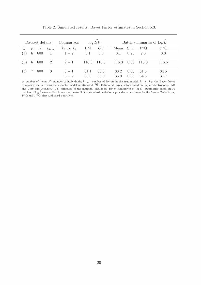
5.3 Computation of Bayes Factor: simulated examples
Here we demonstrate the performance of the CJ estimator using the output from a single runof a multi-block Metropolis-within-Gibbs algorithm, in three simulated datasets of larger size,allowing, in addition, for the models to be fitted with multiple factors of higher dimension.We consider the datasets with the following settings:
a) N = 600 observations with p = 6 items generated from a k = 1 factor model
b) N = 600 observations with p = 6 items generated from a k = 2 factor model
c) N = 800 observations with p = 7 items generated from a k = 3 factor model
All model parameters were selected randomly from a uniform distribution, U(−2, 2). Thenumber of unknown parameters for the posterior ordinate in (15) is equal to k(p + N) + p,corresponding to 606, 1218 and 2428 parameters, respectively, for each of the three situationsdescribed above. Models that either overestimate or underestimate k were also considered,this time evaluating the Bayes factor in favour of the true generating model. Using the sameprocedure as in Section 5.2, we have concluded that it is sufficient to select 30 batches of 1000,2000 and 3000 iterations for the one, two and three-factor models, respectively. All estimatorswere evaluated at the componentwise posterior median (that is, θ∗=posterior median).
The LM estimate of the marginal likelihood is reported as a gold standard using an MCMCoutput of 30,000 iterations, while the log L refers to the estimate of the first batch (of 1,000iterations). The batch mean estimator and the corresponding error were calculated as de-scribed in Section 5. The results in Table 1 suggest that estimates based on the independenceCJ method, proposed in Section 4.1.1, are similar to the ones of the benchmark method (LM),
even from the first batch. Moreover, the Monte Carlo error of the log L is fairly small but nat-urally gets higher as the number of unknown parameters in the posterior ordinate increase fora fixed number of iterations. Nevertheless, this Monte Carlo error can be efficiently reducedby increasing the number of MCMC iterations.
In addition, the one-block (OB) M-H approach described in Section 4.1.2 was implementedfor the second data set (b). The batch mean and the corresponding error were computed over30 batches, as in the case of the multi-block design. In the case where one factor was assumed,the batch mean was logLOB = −2200.68, with MCE(log LOB) = 1.98. In the case where two
factors were assumed, the batch mean was logLOB = −2066.23, with MCE(log LOB) = 3.11.In both cases the estimated log-marginal is far away from the corresponding ones reportedin Table 1 using the LM and the independence CJ estimator. Moreover, under the one-blockdesign, the estimated MCE was 60 and 47 times as high as the corresponding values under themore efficient multi-block design, presented in Table 1. It is therefore verified that betweenthe two single-run approaches, the independence CJ estimator is more efficient and accuratethan the one-block CJ estimator.
13
With regards to the BF, the estimates (in log scale) reported in Table 2 are based on themarginal likelihood estimates presented in Table 1. In all three simulated datasets, theestimated Bayes factors BF indicated the true model. Moreover, when the independence CJwas used, the true model was suggested by the BF estimator at every batch. Bayes factors forthe second and the third dataset clearly indicate the true model, with values ranging from e33
to e116. Only in the first dataset is the Bayes factor much lower and equal to e3 ≈ 20. In thelatter case, or in more extreme cases where two competing models have Bayes factors closeto one, the Monte Carlo error should be small enough in order to be able to identify whichmodel is a-posteriori supported. Here we estimated an error equal to 0.25, with 95% of theestimates ranging between e2.5 = 12.2 and e3.3 = 27.1. Hence, the independence CJ methodinfers safely in favor of the true generating mechanism, providing BF estimates similar to theones obtained from the gold standard of the LM, in all cases.
5.4 Illustration on real data
We proceed with two real-data examples also analyzed in Bartholomew et al. [2, chapter8]. In all examples the marginal likelihood was estimated via CJ I and LM methods at themedian point, over samples of 10 thousand iterations (after discarding 1000 iterations as aburn in period and keeping 1 every 10 iterations to reduce autocorrelations).
The first data set is originally provided by [32] and is part of the Law School Admission Test(LSAT) completed by N = 1005 individuals. The test consists of five items and was designedto measure one latent factor which is also supported by the computed Bayes factor (≈ 0.22and 0.24 for LM and CJ I based estimators, respectively; posterior weight of one-factor model0.802 and 0.817 respectively) reported in the first row of Table 3. In particular, the BF ofthe one-factor versus the two-factor model was less than 0.5 and therefore according to [8]the evidence against the unidimensional model “do not worth more than a bare mention”.
The second data set is part of the 1990 Workplace Industrial Relations Survey (WIRS,[33]). The Bayes factor of the two versus the one-factor model clearly supports the latter(log BF21 ≈ 69); see second line of Table 3. As further analysis, Bartholomew et al. [2]suggested to omit the most poorly fitted item (here item 1) of the scale in order to improvethe fit of the one-factor model. The analysis was replicated for the remaining 5 items tosuggest again the two-factor model as the preferred model (BF21 = 40, that corresponds to“decisive evidence” against the one-factor model, [8]). To summarize, simulations and real-data analysis suggest that the independence CJ estimator succeeds to detect the true model,provides similar estimates to the benchmark method (LM) and has an acceptable MCMCerror.
6 Closing remarks
The paper focused on the CJ [12] marginal likelihood estimator for latent variable models. Inthe popular case where the likelihood expression embodies local independence, conditional onthe latent vector, it was illustrated that the CJ estimator can be computed in a single run ofa Metropolis-within-Gibbs algorithm. This approach drastically reduces the computational
14
effort required for the marginal likelihood estimate. Under conditional independence, thedimensionality of the model is no longer an aspect of the CJ [12] estimator. Hence, thisstrategy can be implemented to reduce the computational time even in models with nolatent variables. That is in models where the likelihood can be augmented using auxiliaryvariables ([17],[34]) to introduce likelihood local independence.
Two more additional points are discussed: (a) the differences of the proposed simplified CJestimator from the (trivial) single-run CJ estimator obtained from one-block Metropolis-Hastings samplers and (b) how we can use the Metropolis kernel to integrate out the latentvariables when no posterior ordinate is analytically available.
The points outlined in this article simplify the implementation of the CJ method on specificcases making a method, which is accurate and already established in bibliography, easier touse and more efficient in practice.
Acknowledgements
This research was funded by the Research Centre of the Athens University of Economics andBusiness.
15
References
[1] I. Moustaki and M. Knott. Generalized latent trait models. Psychometrika, 65:391–411,2000.
[2] D. J. Bartholomew, F. Steele, I. Moustaki, and J. Galbraith. Analysis of MultivariateSocial Science Data. Chapman & Hall/CRC, 2nd edition, 2008.
[3] S. Vitoratou, I. Ntzoufras, N. Smyrnis, and C. N. Stefanis. Factorial composition of theaggression questionnaire: a multi-sample study in greek adults. Psychiatry Research,168(410):32–39, 2009.
[4] I. Moustaki and F. Steele. Latent variable models for mixed categorical and survivalresponses with an application to fertility preferences and family planning in bangladesh.Statistical modelling, 5(4):327–342, December 2005.
[5] I. Moustaki and I. Papageorgiou. Latent class models for mixed variables with appli-cations in archaeometry. Computational Statistics and Data Analysis, 48(3):659–675,2005.
[6] D.J. Bartholomew, M. Knott, and I. Moustaki. Latent variable models and factor anal-ysis: a unified approach. Wiley Series on Probability and Statistics. John Wiley andSons, Ltd, London, 3rd edition, 2011.
[7] R. Patz and B. A. Junker. A straightforward approach to Markov chain Monte Carlomethods for item response models. Journal of Educational and Behavioral Statistics, 24:146–178, 1999.
[8] R.E. Kass and A.E Raftery. Bayes factors. Journal of the American Statistical Associ-ation, 90:773–795, 1995.
[9] S. Chib. Marginal likelihood from the Gibbs output. Journal of the American StatisticalAssociation, 90:1313–1321, 1995.
[10] X.L. Meng and W.H. Wong. Simulating ratios of normalizing constants via a simpleidentity: A theoretical exploration. Statistica Sinica, 6:831–860, 1996.
[11] S.M. Lewis and A.E. Raftery. Estimating Bayes factors via posterior simulation withthe Laplace Metropolis estimator. Journal of the American Statistical Association, 92:648–655, 1997.
[12] S. Chib and I. Jeliazkov. Marginal likelihood from the Metropolis-Hastings output.Journal of the American Statistical Association, 96:270–281, 2001.
[13] N. Friel and A.N. Pettit. Marginal likelihood estimation via power posteriors. Journalof Royal Statistical Society, 770:589–607, 2008.
[14] M.A. Newton and A.E. Raftery. Approximate Bayesian inference with the weightedlikelihood bootstrap. Journal of the Royal Statistical Society, 56:3–48, 1994.
16
[15] D.J. Nott, R. Kohn, and M. Fielding. Approximating the marginal likelihood usingcopula. arXiv:0810.5474v1, 2008. Available at http://arxiv.org/abs/0810.5474v1 .
[16] A. E. Gelfand and A. F. M. Smith. Sampling-based approaches to calculating marginaldensities. Journal of the American Statistical Association, 85(410):398–409, 1990.
[17] M. A. Tanner and W. H. Wong. The calculation of posterior distributions by dataaugmentation. Journal of the American Statistical Association, 82:528–540, 1987.
[18] A. Skrondal and S. Rabe-Hesketh. Generalized Latent Variable Modeling: Multilevel,Longitudinal and Structural Equation Models. Chapman & Hall/CRC, Boca Raton, FL,2004.
[19] J. Geweke and G. Zhou. Measuring the pricing error of the arbitrage pricing theory.Review of Financial Studies, 9:557–87, 1996.
[20] O. Aguilar and M. West. Bayesian dynamic factor models and portfolio allocation.Journal of Business and Economic Statistics, 18:338–357, 2000.
[21] H. F. Lopes and M. West. Bayesian model assessment in factor analysis. StatisticaSinica, 14:4167, 2004.
[22] J. Besag. A candidate’s formula: A curious result in Bayesian prediction. Biometrika,76:183, 1989.
[23] S. Chib and I. Jeliazkov. Inference in semiparametric dynamic models for binary longi-tudinal data. Journal of the American Statistical Association, 101:685–700, 2006.
[24] W.R. Gilks, S. Richardson, and D.J. Spiegelhalter. Introducing markov chan montecarlo. In S. Richardson W.R.Gilks and D.J. Spiegelhalter, editors, Markov Chain MonteCarlo in Practice, pages 165–187. London: Chapman and Hall, 1996.
[25] I. Ntzoufras, P. Dellaportas, and J. Forster. Bayesian variable and link determination forgeneralised linear models. Journal of Statistical Planning and Inference, 111:165–180,2000.
[26] D. Fouskakis, I. Ntzoufras, and D. Draper. Bayesian variable selection using cost-adjusted BIC, with application to cost-effective measurement of quality of health care.Annals of Applied Statistics, 3:663–690, 2009.
[27] S. Rabe-Hesketh, A. Skrondal, and A. Pickles. Maximum likelihood estimation of lim-ited and discrete dependent variable models with nested random effects. Journal ofEconometrics, 128:301–323, 2005.
[28] S. Schilling and R.D Bock. High-dimensional maximum marginal likelihood item factoranalysis by adaptive quadrature. Psychometrika, 70:533–555, 2005.
[29] P. Huber, E. Ronchetti, and M. P. Victoria-Feser. Estimation of generalized linear latentvariable models. Journal of the Royal Statistical Society, Series B, 66:893–908, 2004.
17
[30] B. W. Schmeiser. Batch size effects in the analysis of simulation output. OperationsResearch, 30:556–568, 1982.
[31] P. Bratley, B. L. Fox, and L. E. Schrage. A Guide to Simulation. New York: Springer-Verlag, 1987.
[32] R. D. Bock and M. Lieberman. Fitting a response model for n dichotomously scoreditems. Psychometrika, 35:179–197, 1970.
[33] C. Airey, N. Tremlett, and R. Hamilton. The workplace industrial relations survey 1990.Technical Report (Main and Panel Surveys), Social and Community Planning Research,1992.
[34] D. A. van Dyk and X. L. Meng. The art of data augmentation. Journal of Computationaland Graphical Statistics, 10:1–50, 2001.
18
Tables
Table 1: Simulated results: marginal likelihood estimates in Section 5.3.
Dataset p N ktrue kmodel log LM log L logL MCE(log L)
p: number of items; N : number of individuals; ktrue and kmodel: number of factors in the true andevaluated model, respectively; LM and L: Laplace-Metropolis and Chib and Jeliazkov estimates of themarginal likelihood; logL: Batch mean estimator of the log-marginal likelihood; MCE(log L): Monte Carlo
error of the log L obtained as the standard deviation of 30 batches of equal size as the estimate reported in7th column of the table.
19
Table 2: Simulated results: Bayes Factor estimates in Section 5.3.
Dataset details Comparison log BF Batch summaries of log L
# p N ktrue k1 vs. k2 LM CJ Mean S.D. 1stQ 3rdQ(a) 6 600 1 1 − 2 3.1 3.0 3.1 0.25 2.5 3.3
p: number of items; N : number of individuals; ktrue: number of factors in the true model; k1 vs. k2: the Bayes factor
comparing the k1 versus the k2-factor model is estimated; BF : Estimated Bayes factors based on Laplace-Metropolis (LM)
and Chib and Jeliazkov (CJ) estimates of the marginal likelihood; Batch summaries of log L: Summaries based on 30
batches of log L (mean=Batch mean estimate, S.D.= standard deviation - provides an estimate for the Monte Carlo Error,1stQ and 3rdQ: first and third quartiles).
20
Table 3: Marginal Likelihood and Bayes Factor for the real data: LSAT and WIRS
log LM log L
Dataset 1-factor 2-factor log BF(LM)
21 1-factor 2-factor log BF(CJ)
21
1. LSAT -2494.8 -2496.2 -1.4 -2495.1 -2496.6 -1.52. WIRS-6 items -3456.1 -3387.1 69.0 3456.2 -3387.3 68.93. WIRS-5 items -2786.6 -2782.8 3.8 -2786.8 -2783.1 3.7LM and L: Laplace-Metropolis and Chib and Jeliazkov estimates of the marginal likelihood; 1-factor and 2-factor
columns: estimates of the log-marginal likelihood for the 1-factor and 2-factor models, respectively; BF(LM)
21 and
BF(CJ)
21 : Estimated Bayes factors of 2-factor versus 1-factor model based on LM and L, respectively.
21
Figure labels
Figure 1
Main caption
Ergodic log L using three posterior measures of central location (mean, median and mode)for different M (number of values generated from the proposal) and for different R (numberof MCMC iterations); p=4 items, N = 400 individuals and k=1 latent factor.
Sub captions
Figure 1(a): Sensitivity of log L (based on CJ I) on different M with R = 1000.
Figure 1(b): Sensitivity of log L (based on CJ I) on different R with M = 50.
Figure 2
Main caption
Log-likelihood estimated via CJ I (dotted line) over 30 batches of size R=1000 compared withthe corresponding Laplace-Metropolis estimate (solid line) using MCMC output of 30,000iterations and the posterior median, mean or mode as measures of central location; p=4items, N = 400 individuals and k = 1 factor.