MARINE SURVEY SYSTEM FOR DETECTION OF … ASME Early Career Technical Journal 2009 ASME Early Career...

24.1

ASME Early Career Technical Journal 2009 ASME Early Career Technical Conference, ASME ECTC

October 2-3, 2009, Tuscaloosa, Alabama, USA

MARINE SURVEY SYSTEM FOR DETECTION OF UNEXPLODED ORDNANCE

M. Christopher Gibson, Jim R. McDonald

SAIC, Advanced Sensors and Analysis Division Cary, NC, USA

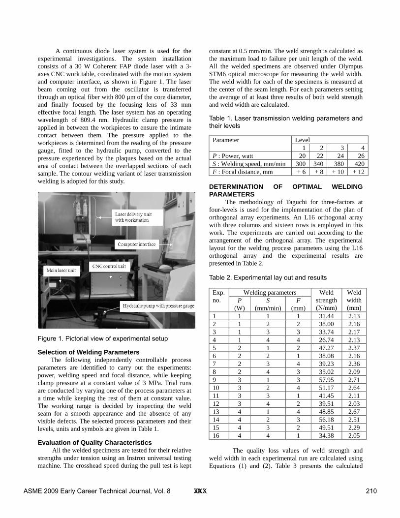
ABSTRACT With support from the Strategic Environmental Research and Development Program (SERDP) and Environment Security Technology and Certification Program (ESTCP), SAIC has developed and demonstrated a marine unexploded ordnance (UXO) survey system designed for use in shallow water (<9.1-m). The air foil shaped sensor platform has two actuator-controlled elevators to control depth, altitude and attitude. The sensor platform incorporates eight cesium vapor magnetometers (0.6-m horizontal spacing) and a time-domain EMI system with a single large transmitter coil and an array of four receiver coils. The sensor platform is towed by a 9.1-m pontoon boat (with a 22-m cable), which houses the data acquisition system and auxiliary electronics required for controlling and monitoring the sensor platform. The sensor platform has two operating modes: altitude mode for maintaining a constant altitude above the bottom; and depth mode for maintaining a constant depth below the water surface. The attitude and depth of the sensor platform is controlled by an autopilot, which feeds output commands to the starboard and port actuators. The autopilot uses attitude information (pitch, roll, and yaw) from a tactical grade inertial measurement unit (IMU) on the sensor platform, velocity data from a real-time-kinematic (RTK) GPS system, heading from the sensor platform magnetic compass, altitude above the bottom from the platform sonar altimeter and water depth from the platform pressure sensor.

The data acquisition system uses a separate GPS unit for synchronization of the system PC clock to GPS UTC time. The system’s first demonstration was at the former Duck Naval Target Range. Approximately 121.4 hectares were surveyed in water depths of 1-4 meters using the magnetometer and EMI sensor arrays. An overall target location accuracy of +/- 30 cm was achieved. A total of 100 targets from the 500 target dig list were reacquired and recovered by UXO- qualified divers. Approximately 50% of the recovered targets were UXO items associated with the former range. Additional surveys have been completed in Ostrich Bay (Puget Sound), Lake Erie(Ohio), bays around Vieques and Culebra islands,( Puerto Rico) and in the Potomac River (off Blossom Point, MD).

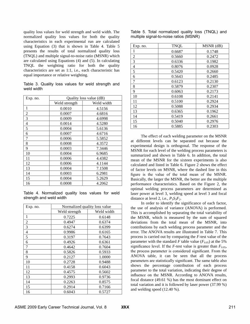
1. INTRODUCTION As a result of current and past military training and weapons-testing activities, Unexploded Ordnance (UXO) is known to be present at many BRAC and FUDS properties and on many active ranges. Many of these sites associated with military practice and test ranges, contain significant land areas with a marine component. Although it is known that between 4 and 8 million hectares of dry land UXO contamination is associated with Closed, Transferred, and Transferring (CTT) ranges, the fraction of this area that is underwater and inaccessible to standard UXO search technologies is poorly defined; however, it likely exceeds a million acres within the continental US. In 2003, with funding from the Strategic Environmental Research and Development Program (SERDP) and the Environment Security Technology Certification Program (ESTCP), SAIC designed and developed the marine-towed array (MTA) UXO sensor system [1,2,3]. This system provides a truly unique capability for underwater UXO search systems. The survey products include digitally geo-referenced magnetic anomaly maps of metallic objects buried in the bottom sediments and estimates of the positions, sizes, and burial depths of the individual metallic anomalies.

2. SENSOR PLATFORM DESIGN

The primary component in the design of the MTA was the sensor platform. The requirements for the operation and performance of the MTA are driven by the sensor requirements for UXO detection. This includes both sensor performance and geometry, sensor positioning and survey speed. Both the magnetometers and the EMI sensors must be isolated from metallic interferences and from electrical and electronic interferences associated with the operation of the sensor platform and the tow vessel. Because of this, construction of the sensor platform must be magnetically clean. Two types of UXO sensors were incorporated in this sensor platform; eight Cesium Vapor magnetometers and a Time Domain Electromagnetic Induction (EMI) system consisting of one (1-m X 4-m) transmitter coil (Tx) and four (0.5-m X 1-m) receiver

ASME 2009 Early Career Technical Journal, Vol. 8 XXX 177

24.2

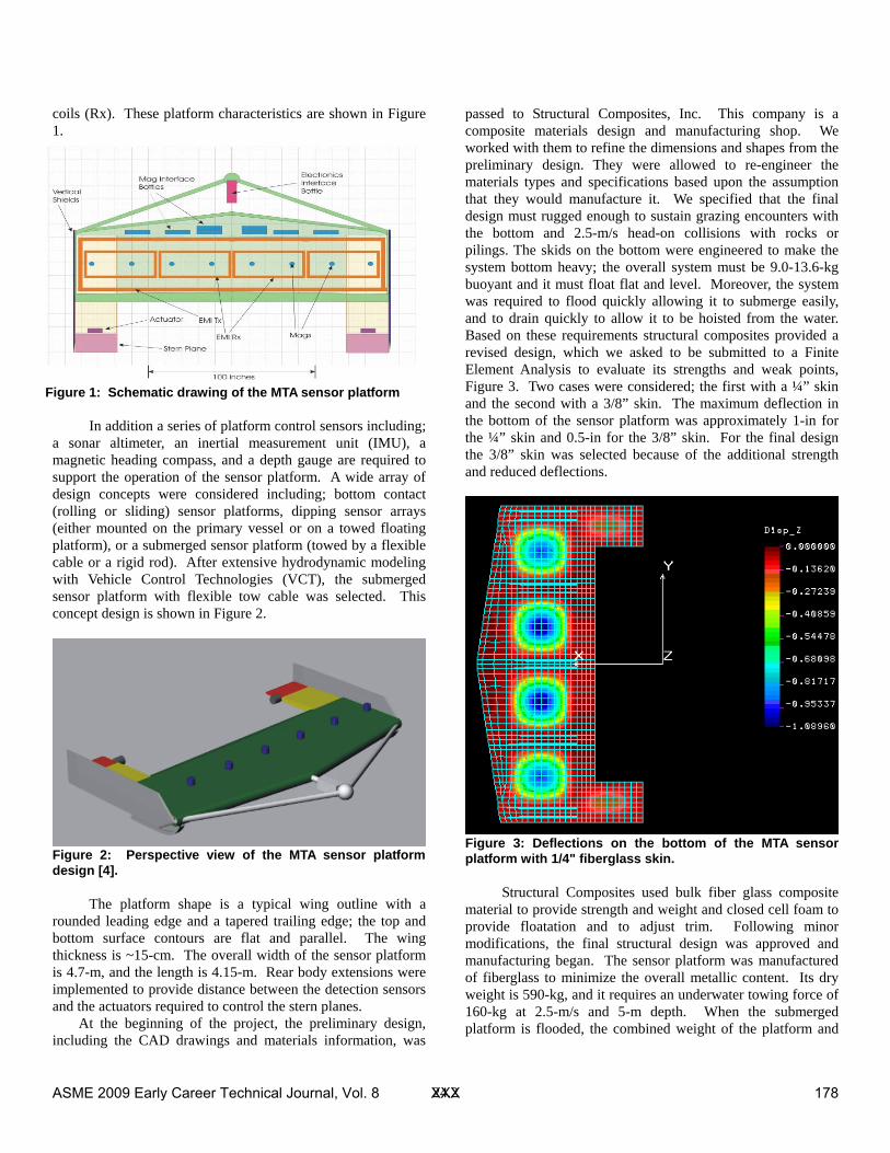
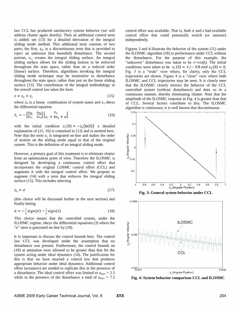
coils (Rx). These platform characteristics are shown in Figure 1.

In addition a series of platform control sensors including;

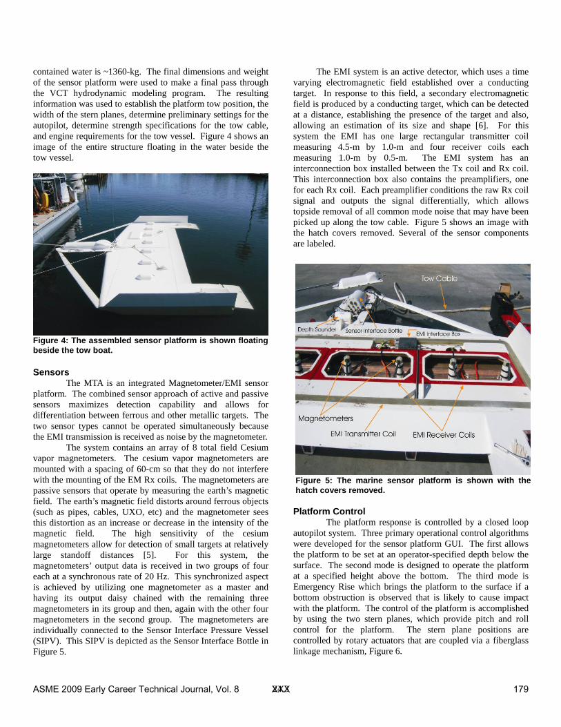
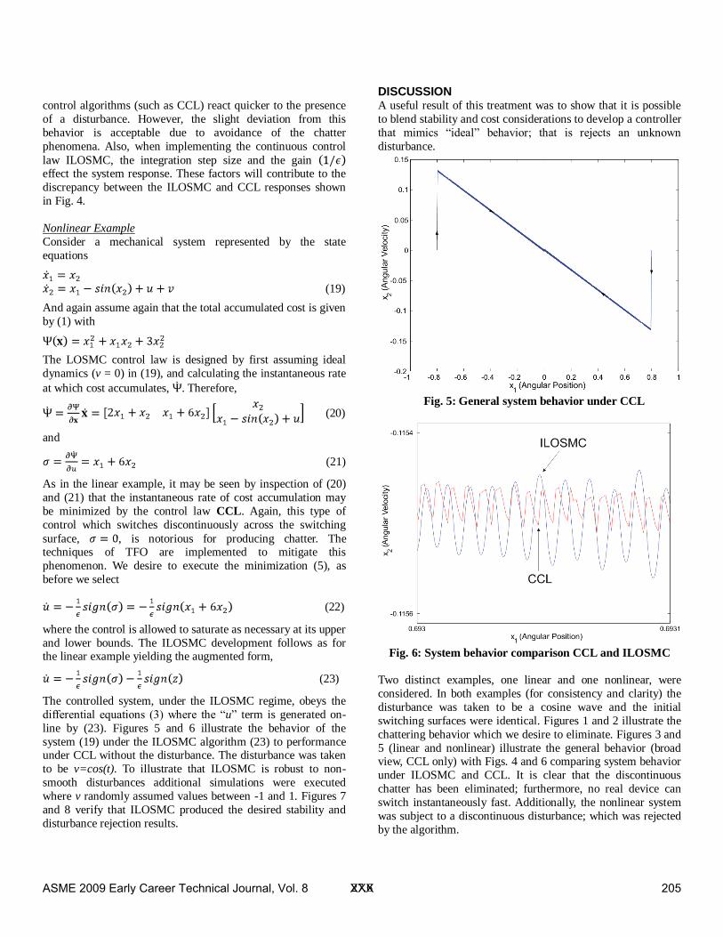
a sonar altimeter, an inertial measurement unit (IMU), a magnetic heading compass, and a depth gauge are required to support the operation of the sensor platform. A wide array of design concepts were considered including; bottom contact (rolling or sliding) sensor platforms, dipping sensor arrays (either mounted on the primary vessel or on a towed floating platform), or a submerged sensor platform (towed by a flexible cable or a rigid rod). After extensive hydrodynamic modeling with Vehicle Control Technologies (VCT), the submerged sensor platform with flexible tow cable was selected. This concept design is shown in Figure 2.

The platform shape is a typical wing outline with a

rounded leading edge and a tapered trailing edge; the top and bottom surface contours are flat and parallel. The wing thickness is ~15-cm. The overall width of the sensor platform is 4.7-m, and the length is 4.15-m. Rear body extensions were implemented to provide distance between the detection sensors and the actuators required to control the stern planes. At the beginning of the project, the preliminary design, including the CAD drawings and materials information, was

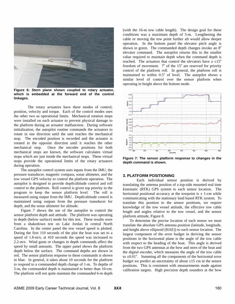
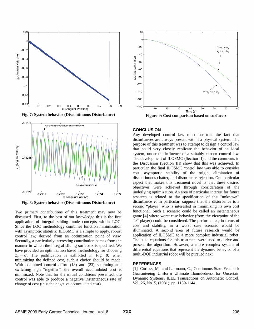
passed to Structural Composites, Inc. This company is a composite materials design and manufacturing shop. We worked with them to refine the dimensions and shapes from the preliminary design. They were allowed to re-engineer the materials types and specifications based upon the assumption that they would manufacture it. We specified that the final design must rugged enough to sustain grazing encounters with the bottom and 2.5-m/s head-on collisions with rocks or pilings. The skids on the bottom were engineered to make the system bottom heavy; the overall system must be 9.0-13.6-kg buoyant and it must float flat and level. Moreover, the system was required to flood quickly allowing it to submerge easily, and to drain quickly to allow it to be hoisted from the water. Based on these requirements structural composites provided a revised design, which we asked to be submitted to a Finite Element Analysis to evaluate its strengths and weak points, Figure 3. Two cases were considered; the first with a ¼” skin and the second with a 3/8” skin. The maximum deflection in the bottom of the sensor platform was approximately 1-in for the ¼” skin and 0.5-in for the 3/8” skin. For the final design the 3/8” skin was selected because of the additional strength and reduced deflections.

Structural Composites used bulk fiber glass composite

material to provide strength and weight and closed cell foam to provide floatation and to adjust trim. Following minor modifications, the final structural design was approved and manufacturing began. The sensor platform was manufactured of fiberglass to minimize the overall metallic content. Its dry weight is 590-kg, and it requires an underwater towing force of 160-kg at 2.5-m/s and 5-m depth. When the submerged platform is flooded, the combined weight of the platform and

Figure 1: Schematic drawing of the MTA sensor platform

Figure 2: Perspective view of the MTA sensor platform design [4].

Figure 3: Deflections on the bottom of the MTA sensor platform with 1/4" fiberglass skin.


24.3

contained water is ~1360-kg. The final dimensions and weight of the sensor platform were used to make a final pass through the VCT hydrodynamic modeling program. The resulting information was used to establish the platform tow position, the width of the stern planes, determine preliminary settings for the autopilot, determine strength specifications for the tow cable, and engine requirements for the tow vessel. Figure 4 shows an image of the entire structure floating in the water beside the tow vessel.

Sensors

The MTA is an integrated Magnetometer/EMI sensor platform. The combined sensor approach of active and passive sensors maximizes detection capability and allows for differentiation between ferrous and other metallic targets. The two sensor types cannot be operated simultaneously because the EMI transmission is received as noise by the magnetometer.

The system contains an array of 8 total field Cesium vapor magnetometers. The cesium vapor magnetometers are mounted with a spacing of 60-cm so that they do not interfere with the mounting of the EM Rx coils. The magnetometers are passive sensors that operate by measuring the earth’s magnetic field. The earth’s magnetic field distorts around ferrous objects (such as pipes, cables, UXO, etc) and the magnetometer sees this distortion as an increase or decrease in the intensity of the magnetic field. The high sensitivity of the cesium magnetometers allow for detection of small targets at relatively large standoff distances [5]. For this system, the magnetometers’ output data is received in two groups of four each at a synchronous rate of 20 Hz. This synchronized aspect is achieved by utilizing one magnetometer as a master and having its output daisy chained with the remaining three magnetometers in its group and then, again with the other four magnetometers in the second group. The magnetometers are individually connected to the Sensor Interface Pressure Vessel (SIPV). This SIPV is depicted as the Sensor Interface Bottle in Figure 5.

The EMI system is an active detector, which uses a time varying electromagnetic field established over a conducting target. In response to this field, a secondary electromagnetic field is produced by a conducting target, which can be detected at a distance, establishing the presence of the target and also, allowing an estimation of its size and shape [6]. For this system the EMI has one large rectangular transmitter coil measuring 4.5-m by 1.0-m and four receiver coils each measuring 1.0-m by 0.5-m. The EMI system has an interconnection box installed between the Tx coil and Rx coil. This interconnection box also contains the preamplifiers, one for each Rx coil. Each preamplifier conditions the raw Rx coil signal and outputs the signal differentially, which allows topside removal of all common mode noise that may have been picked up along the tow cable. Figure 5 shows an image with the hatch covers removed. Several of the sensor components are labeled.

Platform Control

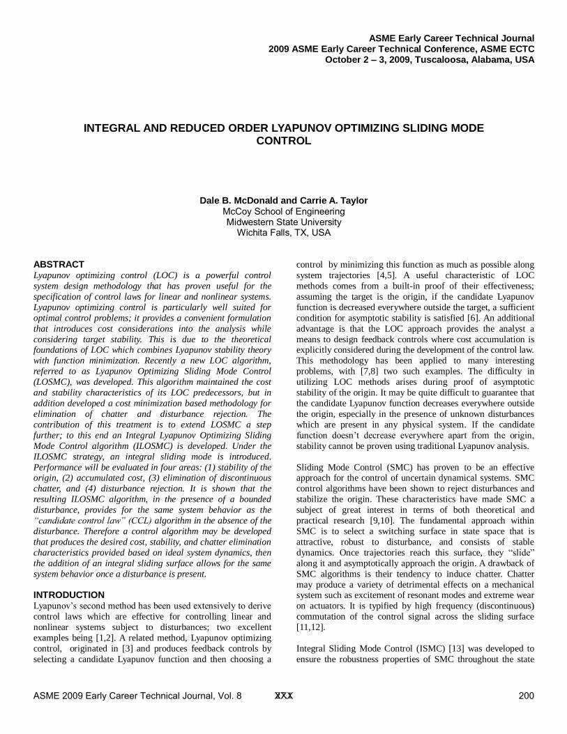
The platform response is controlled by a closed loop autopilot system. Three primary operational control algorithms were developed for the sensor platform GUI. The first allows the platform to be set at an operator-specified depth below the surface. The second mode is designed to operate the platform at a specified height above the bottom. The third mode is Emergency Rise which brings the platform to the surface if a bottom obstruction is observed that is likely to cause impact with the platform. The control of the platform is accomplished by using the two stern planes, which provide pitch and roll control for the platform. The stern plane positions are controlled by rotary actuators that are coupled via a fiberglass linkage mechanism, Figure 6.

Figure 4: The assembled sensor platform is shown floating beside the tow boat.

Figure 5: The marine sensor platform is shown with the hatch covers removed.


24.4

The rotary actuators have three modes of control;

position, velocity and torque. Each of the control modes uses the other two as operational limits. Mechanical rotation stops were installed on each actuator to prevent physical damage to the platform during an actuator malfunction. During software initialization, the autopilot routine commands the actuators to rotate in one direction until the unit reaches the mechanical stop. The encoded position is recorded and the actuator is rotated in the opposite direction until it reaches the other mechanical stop. Once the encoder positions for both mechanical stops are known, the software calculates virtual stops which are just inside the mechanical stops. These virtual stops provide the operational limits of the rotary actuators during operation. The autopilot control system uses inputs from the IMU, the pressure transducer, magnetic compass, sonar altimeter, and the tow vessel GPS velocity to control the platform operation. The autopilot is designed to provide depth/altitude control and roll control to the platform. Roll control is given top priority in the program to keep the sensor platform level. The roll is measured using output from the IMU. Depth/altitude control is maintained using outputs from the pressure transducer for depth, and the sonar altimeter for altitude.

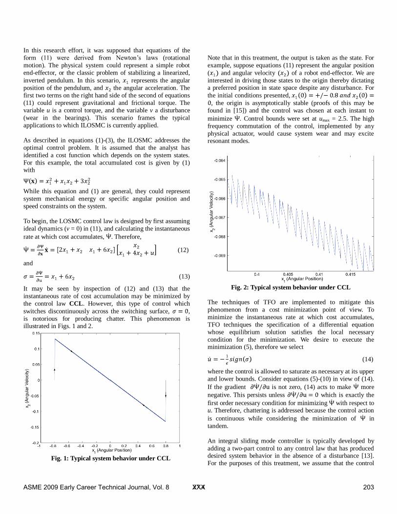
Figure 7 shows the use of the autopilot to control the sensor platform depth and attitude. The platform was operating in depth (below surface) mode for this test. These results were from a shakedown test on Lake Jordan in central North Carolina. In the center panel the tow vessel speed is plotted. During the first 110 seconds of the plot the boat was set to a speed of 1.8-m/s; at 410 seconds the speed was increased to 2.2-m/s. Wind gusts or changes in depth commands affect the speed by small amounts. The upper panel shows the platform depth below the surface. The command depths are shown in red. The sensor platform response to these commands is shown in blue. In general, it takes about 10 seconds for the platform to respond to a commanded depth change of 1-m. To depths of 5-m, the commanded depth is maintained to better than 10-cm. The platform will not quite maintain the commanded 6-m depth

(with the 16-m tow cable length). The design goal for these conditions was a maximum depth of 5-m. Lengthening the cable or moving the tow point further aft would allow deeper operation. In the bottom panel the elevator pitch angle is shown in green. The commanded depth changes invoke an 8o elevator command. The autopilot returns this to the smaller value required to maintain depth when the command depth is reached. The actuators that control the elevators have a ±15o freedom of movement. 7o of the 15o are reserved for priority control of the platform roll. In general, the platform roll is maintained to within 0.5o of level. The autopilot shows a similar level of control over the sensor platform when operating in height above the bottom mode.

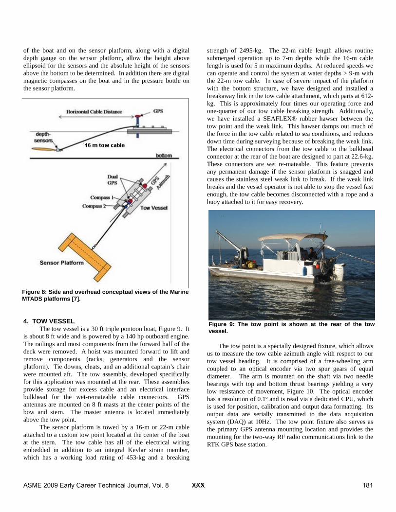
3. PLATFORM POSITIONING Each individual sensor position is derived by translating the antenna position of a top-side mounted real time kinematic (RTK) GPS system to each sensor location. The horizontal positional accuracy at the towpoint is ± 1-cm while communicating with the stationary land based RTK system. To translate this position to the sensor positions, we require knowledge of the tow vessel attitude, the effective tow cable length and angles relative to the tow vessel, and the sensor platform attitude, Figure 8.

To determine the precise location of each sensor we must translate the absolute GPS antenna position (latitude, longitude, and height above ellipsoid [HAE]) to each sensor location. The largest component of the error budget in deriving the sensor positions in the horizontal plane is the angle of the tow cable with respect to the heading of the boat. This angle is derived from the two GPS antennas at the bow and stern of the boat and the digital encoder, which measures the angle of the tow cable to ±0.01o. Summing all the components of the horizontal error budget we predict an uncertainty of about ±15 cm in the sensor positions. This is consistent with measurements made against calibration targets. High precision depth sounders at the bow

Figure 6: Stern plane shown coupled to rotary actuator, which is embedded at the forward end of the control linkages.

Figure 7: The sensor platform response to changes in the depth command is shown.


24.5

of the boat and on the sensor platform, along with a digital depth gauge on the sensor platform, allow the height above ellipsoid for the sensors and the absolute height of the sensors above the bottom to be determined. In addition there are digital magnetic compasses on the boat and in the pressure bottle on the sensor platform.

4. TOW VESSEL

The tow vessel is a 30 ft triple pontoon boat, Figure 9. It is about 8 ft wide and is powered by a 140 hp outboard engine. The railings and most components from the forward half of the deck were removed. A hoist was mounted forward to lift and remove components (racks, generators and the sensor platform). Tie downs, cleats, and an additional captain’s chair were mounted aft. The tow assembly, developed specifically for this application was mounted at the rear. These assemblies provide storage for excess cable and an electrical interface bulkhead for the wet-remateable cable connectors. GPS antennas are mounted on 8 ft masts at the center points of the bow and stern. The master antenna is located immediately above the tow point.

The sensor platform is towed by a 16-m or 22-m cable attached to a custom tow point located at the center of the boat at the stern. The tow cable has all of the electrical wiring embedded in addition to an integral Kevlar strain member, which has a working load rating of 453-kg and a breaking

strength of 2495-kg. The 22-m cable length allows routine submerged operation up to 7-m depths while the 16-m cable length is used for 5 m maximum depths. At reduced speeds we can operate and control the system at water depths > 9-m with the 22-m tow cable. In case of severe impact of the platform with the bottom structure, we have designed and installed a breakaway link in the tow cable attachment, which parts at 612-kg. This is approximately four times our operating force and one-quarter of our tow cable breaking strength. Additionally, we have installed a SEAFLEX® rubber hawser between the tow point and the weak link. This hawser damps out much of the force in the tow cable related to sea conditions, and reduces down time during surveying because of breaking the weak link. The electrical connectors from the tow cable to the bulkhead connector at the rear of the boat are designed to part at 22.6-kg. These connectors are wet re-mateable. This feature prevents any permanent damage if the sensor platform is snagged and causes the stainless steel weak link to break. If the weak link breaks and the vessel operator is not able to stop the vessel fast enough, the tow cable becomes disconnected with a rope and a buoy attached to it for easy recovery.

The tow point is a specially designed fixture, which allows

us to measure the tow cable azimuth angle with respect to our tow vessel heading. It is comprised of a free-wheeling arm coupled to an optical encoder via two spur gears of equal diameter. The arm is mounted on the shaft via two needle bearings with top and bottom thrust bearings yielding a very low resistance of movement, Figure 10. The optical encoder has a resolution of 0.1º and is read via a dedicated CPU, which is used for position, calibration and output data formatting. Its output data are serially transmitted to the data acquisition system (DAQ) at 10Hz. The tow point fixture also serves as the primary GPS antenna mounting location and provides the mounting for the two-way RF radio communications link to the RTK GPS base station.

Figure 8: Side and overhead conceptual views of the Marine MTADS platforms [7].

Figure 9: The tow point is shown at the rear of the tow vessel.


24.6

5. SURVEY OPERATION AND DATA PRODUCTS

The survey is conducted with the information provided by the pilot guidance display unit mounted at the driver’s console, Figure 11.

The survey grid or transects are programmed into the

accompanying computer. The high brightness display can be scaled to guide the driver to the survey area and the beginning transect. The view scrolls as the vessel moves and allows the driver to maintain the course during the survey. The screen also displays the distance off track, the transect number, the GPS fix quality and other information. The water depth, measured by a high precision depth sounder at the bow, is also

displayed to the driver. Under normal survey conditions, an abrupt depth change is displayed to the driver 5-8 seconds before the sensor platform arrives at the same position. All data streams from sensors on the sensor platform and from sensors on the tow vessel are monitored and recorded on one of the three computers in the data acquisition racks, The data are time stamped using GPS Universal Coordinated Time (UTC).

All survey data are typically preprocessed overnight to assure completeness and for quality control purposes. During preprocessing, data are checked for registration, filtered and/or smoothed and vessel turn-arounds are typically edited from the data. The output of this process is a mapped data file suitable for target analysis. If time requirements mandate, one person on site can typically handle the data preprocessing and reduction to an updated mapped data file for next-day analysis. Figure 12 shows a typical block of data from a mapped data image from the survey at Ostrich Bay in Bremerton, WA.

Final work products from the survey include magnetic anomaly maps, target reports containing locations and calculated parameters of size, inclination, azimuth and depth of the analyzed anomalies.

We have carried out extended demonstration surveys on

the Currituck Sound [8] (smooth sand and mud bottom), the protected waters of Ostrich Bay [9] (boulders, broken off pilings, steep walled dredge cuts, 3.6-m tides and water up to 12-m deep), Lake Erie [10] (sand bottom with bedrock outcroppings, cables and pipelines, 1.2-m waves and requirements to operate 19-km off shore), Vieques [11] and Culebra [12], Puerto Rico (open ocean environment, fringing coral reefs, shipwrecks in the survey area, and water up to 12-m deep), and the Potomac River at Blossom Point, Maryland

Figure 10: Tow point showing angular encoder and the break away weak link.

Figure 11: Pilot guidance display showing survey grid .

Figure 12: Magnetic anomaly image (mapped data file) from a ~5 ha area near the center of Ostrich Bay.


24.7

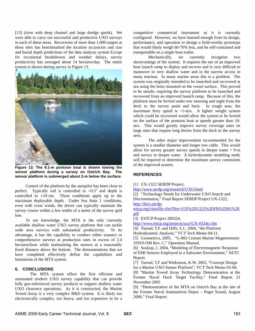
[13] (river with deep channel and large dredge spoils). We were able to carry out successful and productive UXO surveys in each of these areas. Recoveries of more than 1,000 targets at these sites has benchmarked the location accuracies and size and burial depth predictions of the data analysis system Except for occasional breakdowns and weather delays, survey productivity has averaged about 14 hectares/day. The entire system is shown during survey in Figure 13.

Control of the platform by the autopilot has been close to

perfect. Typically roll is controlled to <0.5o and depth is controlled to ±10-cm. These conditions apply up to the maximum deployable depth. Under Sea State 1 conditions, even with cross winds, the driver can typically maintain the survey course within a few tenths of a meter of the survey grid line.

To our knowledge, the MTA is the only currently available shallow water UXO survey platform that can tackle wide area surveys with substantial productivity. To its advantage, it has the capability to conduct either transect or comprehensive surveys at production rates in excess of 2.4 hectares/hour while maintaining the sensors at a reasonably fixed distance above the bottom. The demonstrations that we have completed effectively define the capabilities and limitations of the MTA system. 6. CONCLUSIONS

The MTA system offers the first efficient and automated modern UXO survey capability that can provide fully geo-referenced survey products to support shallow water UXO clearance operations. As it is constructed, the Marine Towed Array is a very complex R&D system. It is likely too electronically complex, too heavy, and too expensive to be a

competitive commercial instrument as it is currently configured. However, we have learned enough from its design, performance, and operation to design a field-worthy prototype that would likely weigh 60-70% less, and be self-contained and transportable on a single boat trailer.

Mechanically, we currently recognize two shortcomings of the system. It requires the use of an improved boat launch ramp to deploy and recover and is very difficult to maneuver in very shallow water and in the narrow access in many marinas. In many marine areas this is a problem. The system was originally intended to be launched and recovered at sea using the hoist mounted on the vessel surface. This proved to be unsafe, requiring the survey platform to be launched and recovered from an improved launch ramp. Because of this, the platform must be ferried under tow morning and night from the dock to the survey point and back. In rough seas, the maximum ferry speed is ~1-m/s. A lighter weight system which could be recovered would allow the system to be ferried on the surface of the pontoon boat at speeds greater than 10-m/s. This would greatly improve survey coverage rates on large sites that require long ferries from the dock to the survey area.

The other major improvement recommended for the system is a smaller diameter and longer tow cable. This would allow for survey greater survey speeds in deeper water > 9-m and survey in deeper water. A hydrodynamic modeling study will be required to determine the maximum survey constraints of the improved system.

REFERENCES

[1] UX-1322 SERDP Project, http://www.serdp.org/research/UXO.html [2] “Technology Needs for Underwater UXO Search and Discrimination,” Final Report SERDP Project UX-1322, http://docs.serdp-estcp.org/viewfile.cfm?Doc=UX%2D1322%2DFR%2D01%2Epdf [3] ESTCP Project 200324, http://www.estcp.org/projects/uxo/UX-0324o.cfm [4] Turead, T.F. and Hills, S.J., 2004, “4m Platform Hydrodynamic Analysis,” VCT Tech Memo 04-11. [5] Geometrics, 2005, “G-882 Cesium Marine Magnetometer 25919-OM Rev. C,” Operation Manual. [6] Soukop, J, 2004, “Modeling of Electromagnetic Response of EMI Sensors Employed in a Saltwater Environment,” AETC Report. [7] Turead, T.F and Watkinson, K.W, 2002, “Concept Design for a Marine UXO Sensor Platform”, VCT Tech Memo 02-06. [8] “Marine Towed Array Technology Demonstration at the Former Naval Duck Target Facility,” Final Report 21 November 2005 [9] “Demonstration of the MTA on Ostrich Bay at the site of the Former Naval Ammunition Depot – Puget Sound, August 2006,” Final Report.

Figure 13: The 9.1-m pontoon boat is shown towing the sensor platform during a survey on Ostrich Bay. The sensor platform is submerged about 2-m below the surface.


24.8

[10] “The MTA UXO Survey and Target Recovery on Lake Erie at the Former Erie Army Depot, ESTCP Project MM2003-24” Final Report, 25 January 2007. [11] “Demonstration of the Marine Towed Array on Bahia Salinas del Sur Vieques, Puerto Rico, June 1-30, 2007”, Final Report, Draft 3 November 2008. [12] “Marine Towed Array (MTA) UXO Geophysical Survey of the Island of Culebra, PR, July 2007,” Final Report, Draft 30 August 2007. [13] “Marine Towed Array Technology Demonstration Blossom Point Research Facility”, Final Report , Draft 15 July 2009.


25.1



IMPROVING THE USABILITY OF LIQUID MOTOR FUELS: THE ACTIVE VAPOR UTILIZATION SYSTEM

Marcus Ashford, Mebougna Drabo, Tad Driver, John Crawford and Michael J. Alff Department of Mechanical Engineering

The University of Alabama Tuscaloosa, Alabama, USA

ABSTRACT The Active Vapor Recovery System (AVUS) was

developed to simultaneously reduce both evaporative and tailpipe emissions from motor vehicles. The AVUS produces liquid fuel from tank vapor generated in normal vehicle operation, for exclusive use during the starting and warm-up periods. The system can process hydrocarbons vapors during refueling, hot soaks, diurnal temperature swings and during normal drives (running losses), considerably reducing evaporative hydrocarbon emissions. The starting fuel produced by AVUS is highly volatile, with a vaporization rate nearly twice that of isopentane, one of the most volatile constituents of pump gasoline. By comparison, the initial boiling point temperature of its parent gasoline corresponds to the temperature at which up to 70% of AVUS condensate will vaporize. The use of AVUS condensate during staring and the subsequent warm-up period will facilitate enhanced combustion and greatly reduced tailpipe emissions during cold starts. The AVUS system can significantly reduce the two most dominant forms of vehicular hydrocarbon emissions simultaneously. No emissions test were conducted for this work, but it is expected that AVUS condensate should facilitate tailpipe hydrocarbon emissions reductions of at least 80%.

INTRODUCTION. Hydrocarbon (HC) emissions are a persistent threat to

the environment. Commonly emitted HC species include precursors to smog formation and agents that are acutely toxic to human, animal and plant life. Moreover, the U.S. Environmental Protection Agency (EPA) reported that automobile sources contributed 44% of the national emissions inventory of volatile organic compounds (VOC) in 2002 [1]. Most VOC emissions released from modern vehicles are generated through incomplete combustion of fuel (tailpipe emissions) and by lost containment of vapors released from fuel on board (evaporative emissions). A few facts bear recognition: (a) The cold-start period, which includes the first 60-90 seconds of engine operation after starting, is responsible

for 60-95% of all tailpipe hydrocarbon emissions during emissions certification testing [2, 3]. (b) Evaporative HC emissions have been conservatively estimated at 3-4x higher than tailpipe emissions during routine driving [4]. (c) Starting fuel generated by the On Board Distillation System – an on-board fuel preprocessor that collected the volatile fractions of gasoline for exclusive use during starting – was demonstrated to reduce overall tailpipe hydrocarbon emissions by more than 80% [2]. One of the conclusions from that study and separate research by Stanglmaier et al [5] was that an ideal starting fuel would be rich in HC species no heavier than C6. (d) As one would expect, the vapor space in a vehicle fuel tank predominantly consists of the lightest fractions of gasoline. Speciation of the vapor above liquid gasoline at 21 °C revealed that the vapor was dominated by three highly volatile species: isobutane (2-methylpropane), n-butane and isopentane (2-methylbutane) collectively accounted for 78% of the vapor composition [6]. (e) Older vehicles have disproportionately higher evaporative and tailpipe hydrocarbon emissions [7-9].

It follows naturally from the preceding statements that significant reductions of hydrocarbon emissions are possible if both evaporative and cold-start tailpipe emissions can be eliminated. It is also apparent that fuel tank vapor makes an excellent starting fuel. Moreover, hydrocarbon emissions from cold starts and fuel evaporation could be reduced or eliminated simultaneously if fuel tank vapors were recovered for use as a starting fuel.

The idea of starting a vehicle with fuel tank vapors is not new; this approach has been attempted many times previously, though with mixed success. Many attempts have been made to develop passive cold starting systems that could induct hydrocarbon vapors from the carbon canister. For the most part these devises tended to suffer from the same fundamental imperfections: (1) there was no way to know conclusively how much vapor could be drawn from the canister; (2) the vapors inducted from the


25.2

carbon canister were mixed with air, and the resultant mixture was of unknown strength; and (3) distributing the vapors evenly among cylinders is very challenging. Predictable and robust fueling is vital for cold-starting, more so than any other operating regime. Thus, most carbon canister vapor induction systems were unsuitable. A promising exception is the Vapor Cold Start System (VCSS) presented by Servati et al [10], which is notable in that it used an active sensor to determine the hydrocarbon concentration in the vapor canister.

A Novel Solution The focus of this research is a new concept for an active

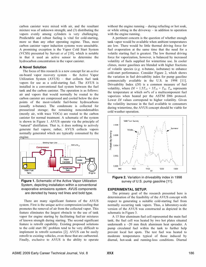
on-board vapor recovery system – the Active Vapor Utilization System (AVUS) – that collects fuel tank vapors for use as a cold-starting fuel. The AVUS is installed in a conventional fuel system between the fuel tank and the carbon canister. The operation is as follows: air and vapors that would normally be routed to the carbon canister are compressed and cooled below the dew points of the most-volatile fuel-borne hydrocarbons (usually n-butane). The condensate is collected for pressurized storage; the remaining noncondensables (mostly air, with trace VOCs) are routed to the carbon canister for normal treatment. A schematic of the system is shown in Figure 1. AVUS operate via the principle of “natural” distillation. That is, it does nothing to actively generate fuel vapors; rather, AVUS collects vapors normally generated which are typically consumed by the engine.

Figure 1. Schematic of the Active Vapor Utilization System, depicting installation within a conventional evaporative emissions system. AVUS components

are denoted by heavy red lines and bold type.

There are many significant features of the AVUS system. First is the unique active compression/cooling that promotes the removal of air from the collected vapor. This feature eliminates the largest obstacle to the use of tank vapor for engine starting by facilitating fuel/air mixtures of known strength during starting. The second significant feature is retrofit capability. Existing proposed solutions to the cold start HC problem tend to be very difficult to implement in retrofit scenarios [2]. AVUS can be easily retrofit to existing vehicles, even those that are carbureted. Finally, exclusive to AVUS is the ability to operate

without the engine running – during refueling or hot soak, or while sitting in the driveway – in addition to operation with the engine running.

A pertinent concern is the question of whether enough tank vapor would be available when ambient temperatures are low. There would be little thermal driving force for fuel evaporation at the same time that the need for a volatile starting fuel is greatest. The low thermal driving force for vaporization, however, is balanced by increased volatility of fuels supplied for wintertime use. In cooler climes, motor gasolines are blended with higher fractions of volatile species (e.g. n-butane, isobutane) to enhance cold-start performance. Consider Figure 2, which shows the variation in fuel driveability index for pump gasoline commercially available in the U.S. in 1998 [11]. Driveability Index (DI) is a common measure of fuel volatility, where DI = 1.5T10 + 3T50 + T90. Tnn represents the temperature at which nn% of a multicomponent fuel vaporizes when heated per the ASTM D86 protocol. Lower DI values correspond to higher volatility. Given the volatility increase in the fuel available to consumers during wintertime, the AVUS concept should be viable for cold weather operation.

Figure 2. Variation in driveability index in 1998

survey of U.S. pump gasoline [11].

EXPERIMENTAL SETUP. The primary goal of the research presented here is

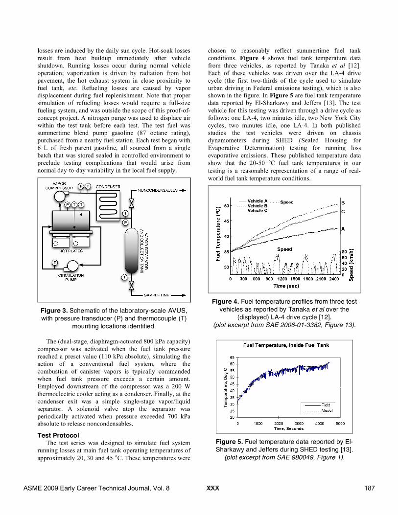
determination of the feasibility of the AVUS concept with respect to generating a suitable cold-starting fuel from normally occurring tank vapors. Thus, a laboratory-scale version of the AVUS was constructed as depicted in the schematic in Figure 3.

A 15 liter aluminum fuel cell represented the main fuel tank; the fuel cell was heated by two hot plates situated underneath a ~20 mm thick aluminum heat spreader. A pump circulated fuel within the tank to further help prevent local hot spots. The test fuel was heated to moderate temperatures typical of those induced by diurnal, hot-soak and running-loss conditions. Diurnal


25.3

losses are induced by the daily sun cycle. Hot-soak losses result from heat buildup immediately after vehicle shutdown. Running losses occur during normal vehicle operation; vaporization is driven by radiation from hot pavement, the hot exhaust system in close proximity to fuel tank, etc. Refueling losses are caused by vapor displacement during fuel replenishment. Note that proper simulation of refueling losses would require a full-size fueling system, and was outside the scope of this proof-of-concept project. A nitrogen purge was used to displace air within the test tank before each test. The test fuel was summertime blend pump gasoline (87 octane rating), purchased from a nearby fuel station. Each test began with 6 L of fresh parent gasoline, all sourced from a single batch that was stored sealed in controlled environment to preclude testing complications that would arise from normal day-to-day variability in the local fuel supply.

Figure 3. Schematic of the laboratory-scale AVUS, with pressure transducer (P) and thermocouple (T)

mounting locations identified.

The (dual-stage, diaphragm-actuated 800 kPa capacity) compressor was activated when the fuel tank pressure reached a preset value (110 kPa absolute), simulating the action of a conventional fuel system, where the combustion of canister vapors is typically commanded when fuel tank pressure exceeds a certain amount. Employed downstream of the compressor was a 200 W thermoelectric cooler acting as a condenser. Finally, at the condenser exit was a simple single-stage vapor/liquid separator. A solenoid valve atop the separator was periodically activated when pressure exceeded 700 kPa absolute to release noncondensables.

Test Protocol The test series was designed to simulate fuel system

running losses at main fuel tank operating temperatures of approximately 20, 30 and 45 °C. These temperatures were

chosen to reasonably reflect summertime fuel tank conditions. Figure 4 shows fuel tank temperature data from three vehicles, as reported by Tanaka et al [12]. Each of these vehicles was driven over the LA-4 drive cycle (the first two-thirds of the cycle used to simulate urban driving in Federal emissions testing), which is also shown in the figure. In Figure 5 are fuel tank temperature data reported by El-Sharkawy and Jeffers [13]. The test vehicle for this testing was driven through a drive cycle as follows: one LA-4, two minutes idle, two New York City cycles, two minutes idle, one LA-4. In both published studies the test vehicles were driven on chassis dynamometers during SHED (Sealed Housing for Evaporative Determination) testing for running loss evaporative emissions. These published temperature data show that the 20-50 °C fuel tank temperatures in our testing is a reasonable representation of a range of real-world fuel tank temperature conditions.

Figure 4. Fuel temperature profiles from three test vehicles as reported by Tanaka et al over the

(displayed) LA-4 drive cycle [12]. (plot excerpt from SAE 2006-01-3382, Figure 13).

Figure 5. Fuel temperature data reported by El-Sharkawy and Jeffers during SHED testing [13].

(plot excerpt from SAE 980049, Figure 1).


25.4

The fuel tank temperature was held constant for the tests, each lasting until at least 500 mL of condensate was generated, or until an hour elapsed. Samples were taken of the parent fuel, the condensate generated and the residual fuel remaining in the main fuel tank. Prior to sample collection, the condensate was chilled to a temperature below 4 °C to minimize vapor loss (AVUS condensate typically boils at room temperature). The parent and residual fuels were sampled at ambient temperature and pressure. Distillation profile testing was performed per ASTM D86 using a Koehler Instruments K45000 Front View Distillation Apparatus. The condensate was Group 0; parent and residual fuels were Group 1. Throughout the duration of AVUS operation and D86 testing, the laboratory ambient temperature was 21 – 22 °C.

Additionally, a simple yet effective volatility test was devised to complement the distillation profile testing. This test – dubbed sTGA – is a simplified version of conventional thermogravimetric analysis. Fuel samples were placed in 4 mL glass cylindrical vials. The sample vials were filled to just below the neck of the bottle, exposing the largest area of liquid possible to air. Because the cross-sectional area of the flask is constant below the neck, the surface area of liquid exposed was constant for the duration of the test. Each the samples was opened and placed on a Sartorius A211P microbalance with the sliding glass doors left open for 40 minutes in a 20 ºC quiescent atmosphere. The room temperature and sample mass were recorded at two-minute intervals.

RESULTS AND DISCUSSION.

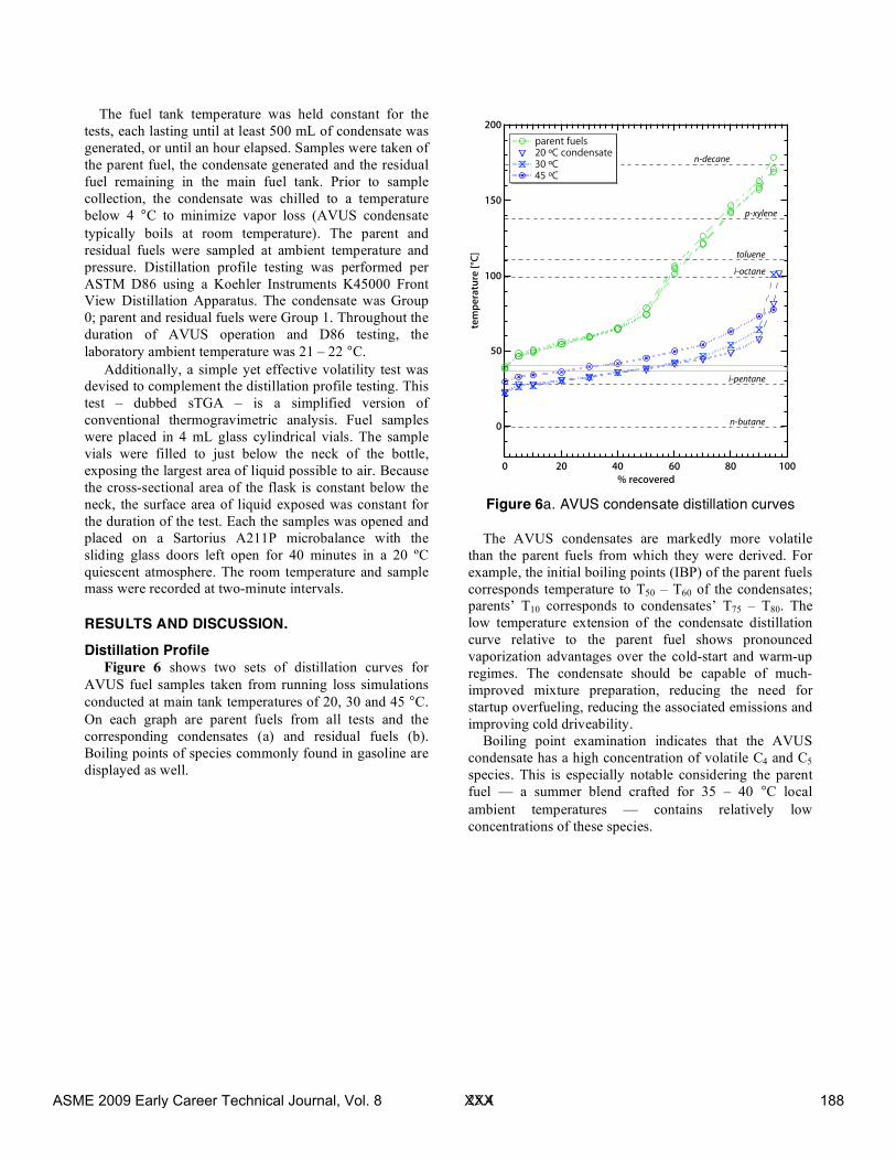
Distillation Profile Figure 6 shows two sets of distillation curves for

AVUS fuel samples taken from running loss simulations conducted at main tank temperatures of 20, 30 and 45 °C. On each graph are parent fuels from all tests and the corresponding condensates (a) and residual fuels (b). Boiling points of species commonly found in gasoline are displayed as well.

200

150

100

50

0

tem

pe

ratu

re [

°C]

100806040200

% recovered

toluene

i-octane

i-pentane

n-butane

p-xylene

n-decane

parent fuels 20 ºC condensate 30 ºC 45 ºC

Figure 6a. AVUS condensate distillation curves

The AVUS condensates are markedly more volatile

than the parent fuels from which they were derived. For example, the initial boiling points (IBP) of the parent fuels corresponds temperature to T50 – T60 of the condensates; parents’ T10 corresponds to condensates’ T75 – T80. The low temperature extension of the condensate distillation curve relative to the parent fuel shows pronounced vaporization advantages over the cold-start and warm-up regimes. The condensate should be capable of much-improved mixture preparation, reducing the need for startup overfueling, reducing the associated emissions and improving cold driveability.

Boiling point examination indicates that the AVUS condensate has a high concentration of volatile C4 and C5 species. This is especially notable considering the parent fuel — a summer blend crafted for 35 – 40 °C local ambient temperatures — contains relatively low concentrations of these species.


25.5

200

150

100

50

0

tem

pe

ratu

re [

°C]

100806040200

% recovered

toluene

i-octane

i-pentane

n-butane

p-xylene

n-decane

parent fuels 20 ºC residual 30 ºC 45 ºC

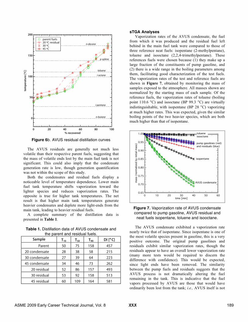
Figure 6b. AVUS residual distillation curves

The AVUS residuals are generally not much less

volatile than their respective parent fuels, suggesting that the mass of volatile ends lost by the main fuel tank is not significant. This could also imply that the condensate generation rate is low, though generation quantification was not within the scope of this study.

Both the condensates and residual fuels display a noticeable level of temperature dependence. Lower main fuel tank temperature shifts vaporization toward the lighter species and reduces vaporization rates. The opposite is true for higher tank temperatures. The net result is that higher main tank temperatures generate heavier condensates and deplete more light-ends from the main tank, leading to heavier residual fuels.

A complete summary of the distillation data is presented in Table 1.

Table 1. Distillation data of AVUS condensate and

the parent and residual fuels. Sample T10 T50 T90 DI [°C]

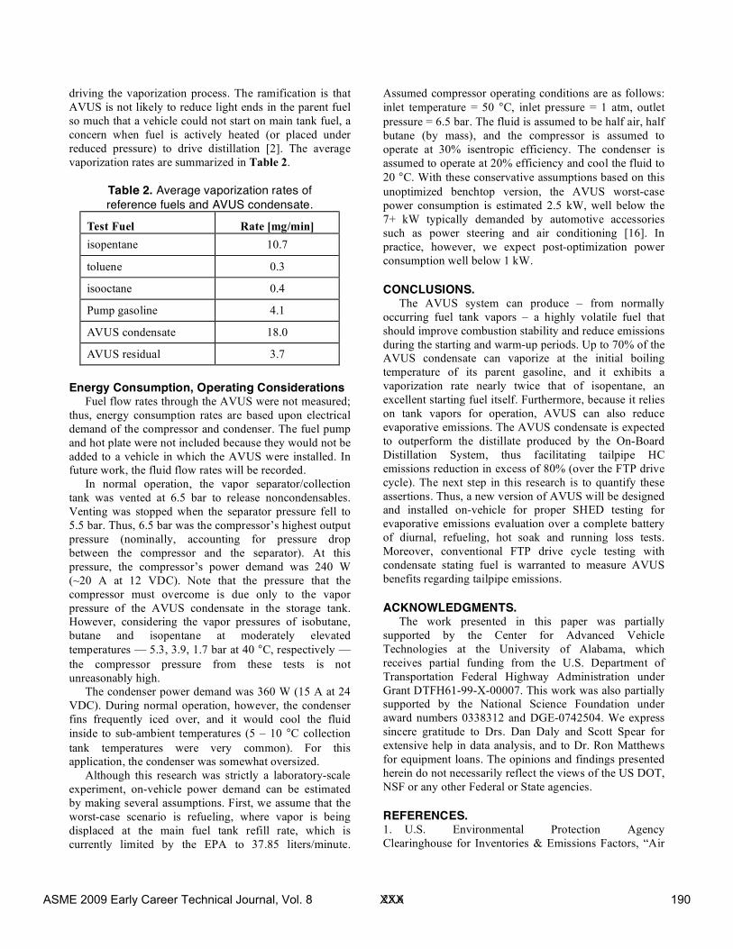
Parent 50 75 158 457 20 condensate 28 38 58 215 30 condensate 27 39 64 223 45 condensate 34 46 73 262

20 residual 52 86 157 493 30 residual 53 92 158 513 45 residual 60 109 164 581

sTGA Analyses Vaporization rates of the AVUS condensate, the fuel

from which it was produced and the residual fuel left behind in the main fuel tank were compared to those of three reference neat fuels: isopentane (2-methylpentane), toluene and isooctane (2,2,4-trimethylpentane). These references fuels were chosen because (1) they make up a large fraction of the constituents of pump gasoline, and (2) there is a wide range in the boiling parameters among them, facilitating good characterization of the test fuels. The vaporization rates of the test and reference fuels are shown in Figure 7, obtained by monitoring the mass of samples exposed to the atmosphere. All masses shown are normalized by the starting mass of each sample. Of the reference fuels, the vaporization rates of toluene (boiling point 110.6 °C) and isooctane (BP 99.3 °C) are virtually indistinguishable, with isopentane (BP 28 °C) vaporizing at much higher rates. This was expected, given the similar boiling points of the two heavier species, which are both much higher than that of isopentane.

1.00

0.95

0.90

0.85

0.80

0.75

0.70

0.65

mass

(norm

aliz

ed b

y init

ial m

ass

)

6050403020100time [min]

tolueneisooctane

pump gasolines (red)and residuals (blue)

isopentane

AVUS condensate

Figure 7. Vaporization rate of AVUS condensate compared to pump gasoline, AVUS residual and

neat fuels isopentane, toluene and isooctane. The AVUS condensate exhibited a vaporization rate

nearly twice that of isopentane. Since isopentane is one of the most volatile species present in gasoline, this is a very positive outcome. The original pump gasolines and residuals exhibit similar vaporization rates, though the residuals appear to have an overall lower vaporization rate (many more tests would be required to discern the difference with confidence). This would be expected, since light ends have been removed. The similarity between the pump fuels and residuals suggests that the AVUS process is not dramatically altering the fuel remaining in the tank. This is indicative that the fuel vapors processed by AVUS are those that would have ordinarily been lost from the tank; i.e., AVUS itself is not


25.6

driving the vaporization process. The ramification is that AVUS is not likely to reduce light ends in the parent fuel so much that a vehicle could not start on main tank fuel, a concern when fuel is actively heated (or placed under reduced pressure) to drive distillation [2]. The average vaporization rates are summarized in Table 2.

Table 2. Average vaporization rates of reference fuels and AVUS condensate.

Test Fuel Rate [mg/min] isopentane 10.7

toluene 0.3

isooctane 0.4

Pump gasoline 4.1

AVUS condensate 18.0

AVUS residual 3.7

Energy Consumption, Operating Considerations Fuel flow rates through the AVUS were not measured;

thus, energy consumption rates are based upon electrical demand of the compressor and condenser. The fuel pump and hot plate were not included because they would not be added to a vehicle in which the AVUS were installed. In future work, the fluid flow rates will be recorded.

In normal operation, the vapor separator/collection tank was vented at 6.5 bar to release noncondensables. Venting was stopped when the separator pressure fell to 5.5 bar. Thus, 6.5 bar was the compressor’s highest output pressure (nominally, accounting for pressure drop between the compressor and the separator). At this pressure, the compressor’s power demand was 240 W (~20 A at 12 VDC). Note that the pressure that the compressor must overcome is due only to the vapor pressure of the AVUS condensate in the storage tank. However, considering the vapor pressures of isobutane, butane and isopentane at moderately elevated temperatures — 5.3, 3.9, 1.7 bar at 40 °C, respectively — the compressor pressure from these tests is not unreasonably high.

The condenser power demand was 360 W (15 A at 24 VDC). During normal operation, however, the condenser fins frequently iced over, and it would cool the fluid inside to sub-ambient temperatures (5 – 10 °C collection tank temperatures were very common). For this application, the condenser was somewhat oversized.

Although this research was strictly a laboratory-scale experiment, on-vehicle power demand can be estimated by making several assumptions. First, we assume that the worst-case scenario is refueling, where vapor is being displaced at the main fuel tank refill rate, which is currently limited by the EPA to 37.85 liters/minute.

Assumed compressor operating conditions are as follows: inlet temperature = 50 °C, inlet pressure = 1 atm, outlet pressure = 6.5 bar. The fluid is assumed to be half air, half butane (by mass), and the compressor is assumed to operate at 30% isentropic efficiency. The condenser is assumed to operate at 20% efficiency and cool the fluid to 20 °C. With these conservative assumptions based on this unoptimized benchtop version, the AVUS worst-case power consumption is estimated 2.5 kW, well below the 7+ kW typically demanded by automotive accessories such as power steering and air conditioning [16]. In practice, however, we expect post-optimization power consumption well below 1 kW.

CONCLUSIONS. The AVUS system can produce – from normally

occurring fuel tank vapors – a highly volatile fuel that should improve combustion stability and reduce emissions during the starting and warm-up periods. Up to 70% of the AVUS condensate can vaporize at the initial boiling temperature of its parent gasoline, and it exhibits a vaporization rate nearly twice that of isopentane, an excellent starting fuel itself. Furthermore, because it relies on tank vapors for operation, AVUS can also reduce evaporative emissions. The AVUS condensate is expected to outperform the distillate produced by the On-Board Distillation System, thus facilitating tailpipe HC emissions reduction in excess of 80% (over the FTP drive cycle). The next step in this research is to quantify these assertions. Thus, a new version of AVUS will be designed and installed on-vehicle for proper SHED testing for evaporative emissions evaluation over a complete battery of diurnal, refueling, hot soak and running loss tests. Moreover, conventional FTP drive cycle testing with condensate stating fuel is warranted to measure AVUS benefits regarding tailpipe emissions.

ACKNOWLEDGMENTS. The work presented in this paper was partially

supported by the Center for Advanced Vehicle Technologies at the University of Alabama, which receives partial funding from the U.S. Department of Transportation Federal Highway Administration under Grant DTFH61-99-X-00007. This work was also partially supported by the National Science Foundation under award numbers 0338312 and DGE-0742504. We express sincere gratitude to Drs. Dan Daly and Scott Spear for extensive help in data analysis, and to Dr. Ron Matthews for equipment loans. The opinions and findings presented herein do not necessarily reflect the views of the US DOT, NSF or any other Federal or State agencies.

REFERENCES. 1. U.S. Environmental Protection Agency Clearinghouse for Inventories & Emissions Factors, “Air


25.7

Pollutant Emission Trends: 1970 - 2002 Average Annual Emissions, All Criteria Pollutants,” January 2005. 2. Ashford, M. D. and Matthews, R.D. “On-Board Generation Further Development of a Highly Volatile Starting Fuel to Reduce Automobile Cold-Start Emissions,” Environmental Science and Technology, 40:5770-5777, 2006. 3. Kidokoro, T., K. Hoshi, K. Hiraku, K. Satoya, T. Watanabe, T. Fujiwara and H. Suzuki “Development of PZEV Exhaust Emission Control System,” SAE 2003-01-0817. 4. Lyons, J., Lee, J., Heirigs, P., McClement, D. and Steve Welstand, S., “Evaporative Emissions from Late-Model In-Use Vehicles,” SAE 2000-01-2958. 5. Stanglmaier, R., Roberts, C., Ezekoye, O. and Matthews, R., “Condensation of Fuel on Combustion Chamber Surfaces as a Mechanism for Increased HC Emissions During Cold Start,” SAE 972884. 6. Siegl, W., Guenther, M. and Henney, T., “Identifying Sources of Evaporative Emissions – Using Hydrocarbon Profiles to Identify Emission Sources,” SAE 2000-01-1139. 7. California Air Resources Board, www.arb.ca.gov. 8. South Coast Air Quality Management District, www.aqmd.gov.

9. Davis, D. L., When Smoke Ran Like Water: Tales of Environmental Deception and the Battle Against Pollution, Basic Books, New York, 2002. 10. Servati, H., Marshall, S., Murphy, J., Sanei, M. F., Zhou W. and Lewis, W., “Carbon Canister-Based Vapor Management System to Reduce Cold-Start Hydrocarbon Emissions,” SAE 2005-01-3866. 11. Lambert, D. K., Harrington, C. R., Kerr R., Lee, H., Lin, Y., Wang, D. Y., and Wang, S. “Fuel Driveability Index Sensor,” SAE 2003-01-3238. 12. Tanaka, H., Kaneko, T., Matsumoto, T., Kato, T. and Takeda, H., “Effects of Ethanol and ETBE Blending in Gasoline on Evaporative Emissions,” SAE 2006-01-3382. 13. El-Sharkawy, A. E., Jeffers, J., “Transient Fuel System Thermal and Emissions Analysis,” SAE 980049. 14. Huber M. L. (National Institute of Standards and Technology) “NIST Thermophysical Properties of Hydrocarbon Mixtures Database (SUPERTRAPP), Version 3.2,” 2007. 15. Chevron Products Company, “Motor Gasolines Technical Review,” 2009. 16. Kluger, M and Harris, J “Fuel Economy Benefits of Electric and Hydraulic Off Engine Accessories,” SAE 2007-01-0268.


26.1



IMPROVING THE USABILITY OF LIQUID MOTOR FUELS: PREDICTING FUEL VOLATILITY VIA ARTIFICIAL INTELLIGENCE

PART I – NUMERICAL SIMULATION

Tad Driver and Marcus Ashford The University of Alabama Tuscaloosa, Alabama, USA

ABSTRACT A relatively simple phase equilibrium algorithm has

been demonstrated to have the capability to predict a liquid fuel composition for a surrogate (synthetic) fuel, given the corresponding hydrocarbon vapor concentration. Ideal gas and liquid behavior was assumed to reduce computational overhead. The result was that the model was most accurate (< 1% error compared to NIST SUPERTRAPP) when predicting compositions of closely related HC species. Interchangeability among surrogate species predicted by the model was experimentally verified with respect to vaporization, proving that boiling point range is the property of most importance when selecting surrogate fuel species. Experimental studies are currently underway to verify the model’s accuracy in real and simulated engine fuel/air preparations systems. Future work will include incorporation of real-fluid behavior into the model to improve prediction accuracy for dissimilar hydrocarbons and in operating conditions near the single-phase regions for given mixtures.

INTRODUCTION Automobiles are responsible for a significant portion

of hydrocarbons (HC) released to the environment. In 2002, the US Environmental Protection Agency estimated that mobile sources were responsible for 44% of the national inventory of volatile organic compounds [1]. The majority of hydrocarbon combustion emissions from on-road vehicles occur during transient operation, particularly cold-starts (engine at ambient temperature), during which temperature and pressure within the engine are rapidly changing. Measured over the industry standard FTP protocol, 60 – 95% of all tailpipe HC emissions occur during the first 60 – 90 seconds after start [2-4]. One of the root causes is gasoline’s relatively low volatility and associated poor fuel vaporization. At moderate temperatures, only 10 – 30% of the injected fuel vaporizes and joins the combustible mix [3], necessitating generous over-fueling to achieve robust starting. Moreover, the volatility of commercially available pump gasoline varies considerably both geographically and seasonally. Figure

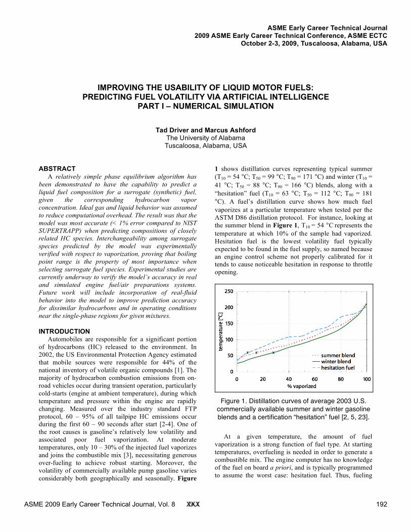
1 shows distillation curves representing typical summer (T10 = 54 °C; T50 = 99 °C; T90 = 171 °C) and winter (T10 = 41 °C; T50 = 88 °C; T90 = 166 °C) blends, along with a “hesitation” fuel (T10 = 63 °C; T50 = 112 °C; T90 = 181 °C). A fuel’s distillation curve shows how much fuel vaporizes at a particular temperature when tested per the ASTM D86 distillation protocol. For instance, looking at the summer blend in Figure 1, T10 = 54 °C represents the temperature at which 10% of the sample had vaporized. Hesitation fuel is the lowest volatility fuel typically expected to be found in the fuel supply, so named because an engine control scheme not properly calibrated for it tends to cause noticeable hesitation in response to throttle opening.

Figure 1. Distillation curves of average 2003 U.S.

commercially available summer and winter gasoline blends and a certification “hesitation” fuel [2, 5, 23].

At a given temperature, the amount of fuel

vaporization is a strong function of fuel type. At starting temperatures, overfueling is needed in order to generate a combustible mix. The engine computer has no knowledge of the fuel on board a priori, and is typically programmed to assume the worst case: hesitation fuel. Thus, fueling


26.2

during a cold start can be 10 – 20 times the stoichiometric amount [2-4].

The problem of fueling inaccuracy is not limited to the cold start transient. Even in an engine at operating temperature, some of the injected fuel will join intake port and/or in-cylinder fuel films. The mass and mass rate of change of these fuel films is a function of temperature, pressure and fuel composition. During throttle-opening transients (increasing intake pressure), the film mass grows, creating a lean excursion unless additional fuel is injected as compensation. Conversely, during throttle-closing transients, the decreasing fuel film mass will cause rich excursions. These air-fuel excursions increase emissions and fuel consumption while decreasing driveability. Modern engine controllers have transient fuel compensation capability, but it is clear that a control scheme that employs knowledge of the fuel distillation profile would be beneficial in reducing transient fueling complications in all transient operating conditions.

This research is part of a larger program with the goal of improving emissions, fuel consumption and driveability by increasing the capability of an engine controller to understand liquid/vapor fuel dynamics. Specifically, the research discussed here aims to develop engine control schemes that employ a more complete “understanding” of fuel volatility. An engine computer armed with compositional information and the means to perform volatility calculations should be capable of significantly improved fueling accuracy. However, motor fuels are specified by distillation profile rather than composition, and they typically contain hundreds of constituents. Modern engine controllers do not possess sufficient computing power to calculate volatility from that many components, certainly not in real time. A simplified approach is necessary.

Problem Statement Several techniques for estimating fuel volatility at

engine operating conditions have been developed. Most of these models employ surrogate fuels with a limited (<20) number of components to represent gasoline [3, 5, 6]. These models tend to be empirical in nature, requiring unique calibrations for each engine to which the model is applied.

The paramount goal of this work is to develop an algorithm that can calculate fuel volatility via the principles of phase equilibrium. More specifically, if the HC vapor concentration (in a volume of air) is known, the algorithm is tasked with accurately predicting the composition of the pre-equilibrium liquid fuel from which the vapor would have emanated. In practice, the most desirable method for determining HC vapor concentration will be via interpretation of post-combustion oxygen sensor readings. Alternatively, an inexpensive in-tank HC sensor could be employed. Immediate plans are to use fast-FID sensing to collect experimental data for

algorithm validation. The problem statement is illustrated schematically in Figure 2. A chief requirement of this algorithm is low computing overhead; real-time operation (~ engine cycle frequencies) is highly desired.

Figure 2. Depiction of the problem statement

This is the first in a series of manuscripts detailing the research and development of the control algorithm and its accompanying engine controller. This paper describes initial proof of concept testing of the routine and selection of the potential surrogate fuel ingredients. The basic algorithm is comprised of two modules, a cubic equation of state for predicting phase equilibrium and artificial intelligence to determine fuel composition. The 1978 version of the Peng-Robinson Equation of State (EOS) (hereafter referred to as PR78) is employed for phase equilibrium calculations [7, 8]; particle swarm optimization is the foundation of the AI engine.

Particle Swarm Optimization Particle Swarm Optimization (PSO) is a stochastic

artificial intelligence problem solving technique. PSO is a type of swarm intelligence, which generally describes problem-solving techniques displayed by social animals. Essentially, group members (particles) react to the actions of their fellow members as the population collectively solves a problem. Particularly, PSO is inspired by animal social behaviors such as bird flocks, fish schools or swarms of flies. Kennedy et al describe PSO succinctly as “evaluate, compare, imitate” [9].

Many aspects of PSO are similar to more popular AI techniques, such as genetic algorithms (GA). Populations of particles are seeded; each particle within the population is repeatedly evaluated for fitness; and successive generations yield improved results. However, in PSO,


26.3

each particle is “self-aware” and possesses awareness of the other members of its population. Each particle knows its current coordinates and value; its personal best coordinates and value (pbest); and the overall best coordinates and value for the global population (gbest). Each particle constantly adjusts its heading in a direction toward pbest and gbest.

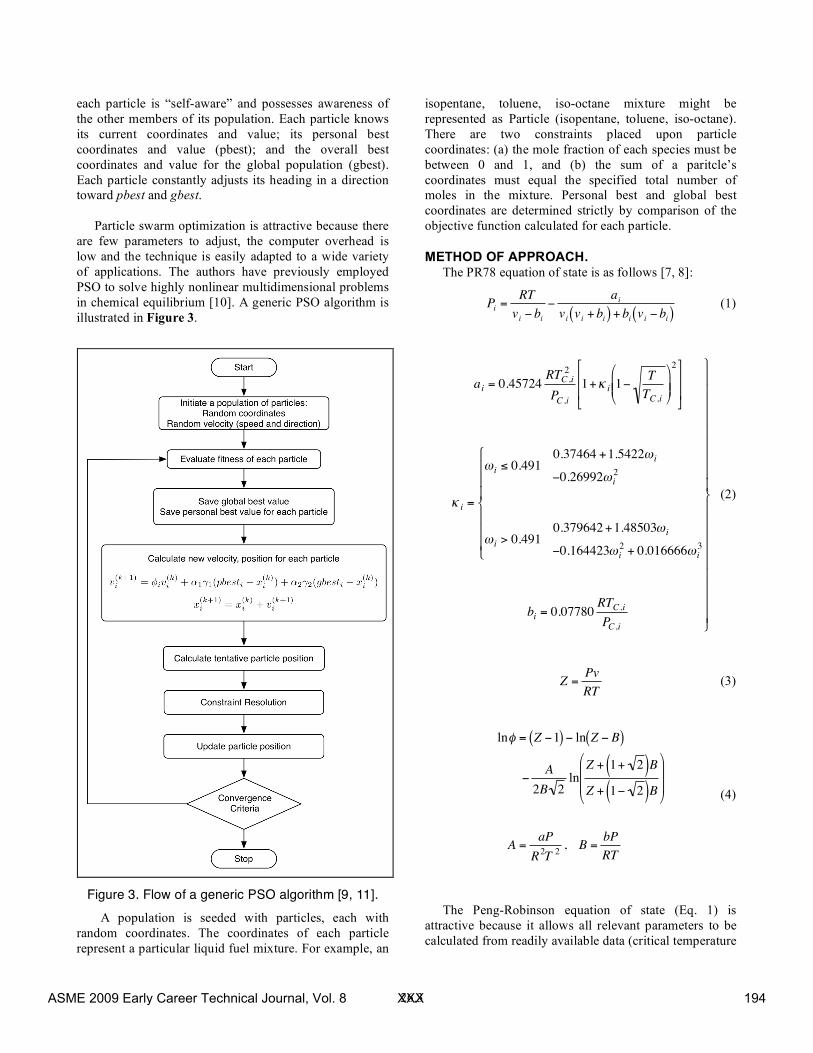
Particle swarm optimization is attractive because there are few parameters to adjust, the computer overhead is low and the technique is easily adapted to a wide variety of applications. The authors have previously employed PSO to solve highly nonlinear multidimensional problems in chemical equilibrium [10]. A generic PSO algorithm is illustrated in Figure 3.

Figure 3. Flow of a generic PSO algorithm [9, 11].

A population is seeded with particles, each with random coordinates. The coordinates of each particle represent a particular liquid fuel mixture. For example, an

isopentane, toluene, iso-octane mixture might be represented as Particle (isopentane, toluene, iso-octane). There are two constraints placed upon particle coordinates: (a) the mole fraction of each species must be between 0 and 1, and (b) the sum of a paritcle’s coordinates must equal the specified total number of moles in the mixture. Personal best and global best coordinates are determined strictly by comparison of the objective function calculated for each particle.

METHOD OF APPROACH. The PR78 equation of state is as follows [7, 8]:

!

Pi=

RT

vi" b

i

"ai

vivi+ b

i( ) + bivi" b

i( ) (1)

!

ai

= 0.45724RT

C ,i2

PC ,i

1+"i1#

T

TC ,i

$

% & &

'

( ) )

2*

+

, ,

-

.

/ /

"i

=

0i1 0.491

0.37464 +1.54220i

#0.269920i

2

0i> 0.491

0.379642+1.485030i

#0.1644230i

2+ 0.0166660

i

3

2

3

4 4 4

5

4 4 4

bi

= 0.07780RT

C ,i

PC ,i

6

7

4 4 4 4 4 4 4 4 4

8

4 4 4 4 4 4 4 4 4

(2)

!

Z =Pv

RT (3)

!

ln" = Z #1( ) # ln Z # B( )

#A

2B 2ln

Z + 1+ 2( )BZ + 1# 2( )B

$

%

& &

'

(

) )

A =aP

R2T2, B =

bP

RT

(4)

The Peng-Robinson equation of state (Eq. 1) is attractive because it allows all relevant parameters to be calculated from readily available data (critical temperature


26.4

Tc, critical pressure Pc and acentric factor ω). Equation 2 represents the Peng-Robinson attraction parameter (a), the covolume of the mixture (b), and the constant characteristic of each substance (κi ), which are all used to determine the state of the composition. The goal is to calculate the fugacity ratio (Eq. 4) of the mixture. Fugacity is a measure of the tendency of a substance to migrate to one state over another. The fugacity ratios ϕ for liquid and vapor phases are calculated from compressibility factor Z (Eq. 3) at the given temperature and pressure to determine the equilibrium ratio

!

keq ="vapor

" liquid=y

x, (5)

which defines the ratio of the mole fractions of each component in each phase of the mixture. In the equations above, the terms A and B only serve to simplify the compressibility factor equation.

In this first version of the algorithm, ideal gas and ideal liquid behavior are assumed. This greatly reduces computational overhead at the risk of decreased accuracy. However, ideal-behavior-assumption accuracy improves with similarity of the species involved, and is generally acceptable with light hydrocarbons [12, 13]. The constituents of motor gasoline are hydrocarbons in a relatively narrow carbon number range (C4 – C12); despite this, should the surrogate mixture include paraffins, olefins, aromatics, air, etc., accuracy can rapidly deteriorate. If necessary, later iteration of the algorithm will consider real-fluid phase equilibrium calculation techniques such as those presented by Jaubert et al [14-18].

Air is assumed to consist only of diatomic nitrogen, due to N2 comprising ~80% of air by volume. The HC concentration of the vapor is a pure HC concentration, meaning that it is just the sum of all the HC molecules, in the vapor, from the different fuelsj, and not the type of concentration one gets from a HC analyzer that represents HCs in terms of a particular HC (e.g. ppm-C1). The objective function to be minimized was

!

HCt arg et "HCactual

. (6)

HCtarget represents the desired HC concentration input into the algorithm, where as HCactual is the concentration calculated by the algorithm for each fuel composition. The overall convergence criterion was that the absolute value of the difference between these two was within 0.01% of the target concentration.

In order to test the accuracy of the algorithm, its predicted fuel mixtures were input into the NIST SUPERTRAPP [20] vapor-liquid equilibrium program to compare calculated HC concentrations. Tests were conducted with binary, ternary and quinary fuel blends.

The target HC concentrations were varied throughout the 2-phase liquid-vapor region of each fuel blend simulated. Also, each fuel blend was tested at 3 different temperatures (273, 288 and 300 K) to simulate typical cold start operating conditions. Note, the pressure was held constant at 100,000 Pa throughout all the tests. This was done because the initial pressure for engine starts is typically atmospheric pressure. Each test was conducted five times to check for repeatability. The SUPERTRAPP computations are considered the reference standard here, as its accuracy has been demonstrated in the literature [3, 19].

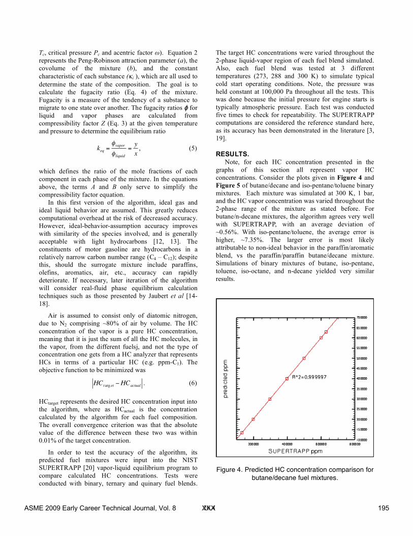
RESULTS. Note, for each HC concentration presented in the

graphs of this section all represent vapor HC concentrations. Consider the plots given in Figure 4 and Figure 5 of butane/decane and iso-pentane/toluene binary mixtures. Each mixture was simulated at 300 K, 1 bar, and the HC vapor concentration was varied throughout the 2-phase range of the mixture as stated before. For butane/n-decane mixtures, the algorithm agrees very well with SUPERTRAPP, with an average deviation of ~0.56%. With iso-pentane/toluene, the average error is higher, ~7.35%. The larger error is most likely attributable to non-ideal behavior in the paraffin/aromatic blend, vs the paraffin/paraffin butane/decane mixture. Simulations of binary mixtures of butane, iso-pentane, toluene, iso-octane, and n-decane yielded very similar results.

Figure 4. Predicted HC concentration comparison for

butane/decane fuel mixtures.


26.5

Figure 5. Predicted HC concentration comparison for

isopentane/toluene fuel mixtures.

As stated before, each of the mixtures were also tested at 288 K and 273 K. For each mixture, the accuracy of the model decreased with decreasing temperature. For instance, the average deviation for the butane/n-decane mixture is presented in Table 1. It is clear that the accuracy of the algorithm decreases with temperature. All the other mixtures tested exhibited the same exact behavior. This accuracy loss can be directly attributed to the ideal gas/liquid assumptions of the model, which are less valid at lower temperatures, especially at temperatures below the boiling points of all constituents of the mixture, near the mixture single-phase regions.

Table 1. Average deviation of butane/n-decane mixture

273 K 288 K 300 K Average Deviation 1.75 % 1.13 % 0.56 %

The next phase of simulation involved quinary fuel

mixture, in expectation that any viable gasoline surrogate would require at least five components to accurately model the gasoline distillation profile. The proposed mixture ingredients were butane, isopentane (methylbutane), toluene, iso-octane (2,2,4-trimethylpentane) and decane, chosen because they collectively account for the majority the content of commercially available pump gasoline. Moreover, these components span most of the boiling point range of

gasoline. The simulations were conducted for 300 K, 1 bar. Figure 6 shows that there are many possible “recipes” of the given species that can yield a HC concentration of 300,000 ppm. The number of combinations is quite possibly infinite. Verification of the Figure 6 blends is shown in Figure 7, which shows the predicted HC concentration of the algorithm versus that calculated by SUPERTRAPP. Looking at Figure 7, the 5 simulations run at 300,000 ppm all lie very close to the linear trend of the simulations, thus proving all the mixtures predicted by the code are legitimate.

At first glance of Figure 6 the predicted mixtures seem to be somewhat random, which would seem to suggest that the code need be constrained to certain mole number ranges for each species in order to avoid randomness. Closer inspection, however, reveals it seems that species with similar boiling points can be interchanged. In this particular case, the code seems to be swapping the butane and iso-pentane between the different simulations.

Figure 6. Quinary mixtures of butane, iso-pentane,

toluene, iso-octane, and n-decane. HC concentration is 300,000 ppm


26.6

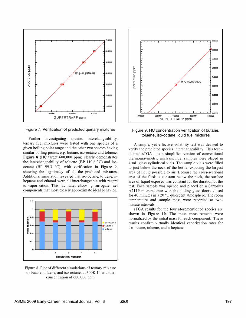
Figure 7. Verification of predicted quinary mixtures

Further investigating species interchangeability,

ternary fuel mixtures were tested with one species of a given boiling point range and the other two species having similar boiling points, e.g, butane, iso-octane and toluene. Figure 8 (HC target 600,000 ppm) clearly demonstrates the interchangeability of toluene (BP 110.6 °C) and iso-octane (BP 99.3 °C), with verification in Figure 9, showing the legitimacy of all the predicted mixtures. Additional simulation revealed that iso-octane, toluene, n-heptane and ethanol were all interchangeable with regard to vaporization. This facilitates choosing surrogate fuel components that most closely approximate ideal behavior.

Figure 8. Plot of different simulations of ternary mixture of butane, toluene, and iso-octane, at 300K,1 bar and a

concentration of 600,000 ppm

Figure 9. HC concentration verification of butane,

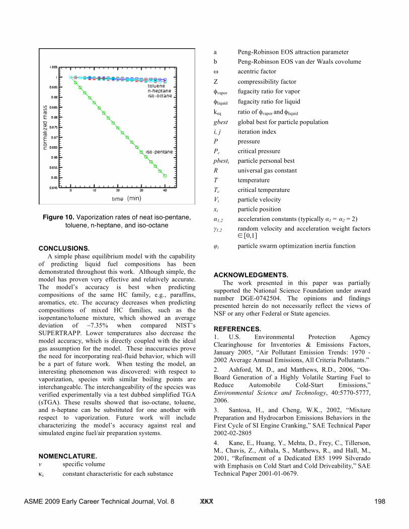
toluene, iso-octane liquid fuel mixtures A simple, yet effective volatility test was devised to

verify the predicted species interchangeability. This test – dubbed sTGA – is a simplified version of conventional thermogravimetric analysis. Fuel samples were placed in 4 mL glass cylindrical vials. The sample vials were filled to just below the neck of the bottle, exposing the largest area of liquid possible to air. Because the cross-sectional area of the flask is constant below the neck, the surface area of liquid exposed was constant for the duration of the test. Each sample was opened and placed on a Sartorius A211P microbalance with the sliding glass doors closed for 40 minutes in a 20 ºC quiescent atmosphere. The room temperature and sample mass were recorded at two-minute intervals.

sTGA results for the four aforementioned species are shown in Figure 10. The mass measurements were normalized by the initial mass for each component. These results confirm virtually identical vaporization rates for iso-octane, toluene, and n-heptane.


26.7

Figure 10. Vaporization rates of neat iso-pentane,

toluene, n-heptane, and iso-octane

CONCLUSIONS. A simple phase equilibrium model with the capability

of predicting liquid fuel compositions has been demonstrated throughout this work. Although simple, the model has proven very effective and relatively accurate. The model’s accuracy is best when predicting compositions of the same HC family, e.g., paraffins, aromatics, etc. The accuracy decreases when predicting compositions of mixed HC families, such as the isopentane/toluene mixture, which showed an average deviation of ~7.35% when compared NIST’s SUPERTRAPP. Lower temperatures also decrease the model accuracy, which is directly coupled with the ideal gas assumption for the model. These inaccuracies prove the need for incorporating real-fluid behavior, which will be a part of future work. When testing the model, an interesting phenomenon was discovered: with respect to vaporization, species with similar boiling points are interchangeable. The interchangeability of the species was verified experimentally via a test dubbed simplified TGA (sTGA). These results showed that iso-octane, toluene, and n-heptane can be substituted for one another with respect to vaporization. Future work will include characterizing the model’s accuracy against real and simulated engine fuel/air preparation systems.

NOMENCLATURE. v specific volume κi constant characteristic for each substance

a Peng-Robinson EOS attraction parameter b Peng-Robinson EOS van der Waals covolume ω acentric factor Z compressibility factor φvapor fugacity ratio for vapor φliquid fugacity ratio for liquid keq ratio of φvapor and φliquid gbest global best for particle population i, j iteration index P pressure Pc critical pressure pbesti particle personal best R universal gas constant T temperature Tc critical temperature Vi particle velocity xi particle position α1,2 acceleration constants (typically α1 = α2 = 2) γ1,2 random velocity and acceleration weight factors

∈ [0,1] φi particle swarm optimization inertia function

ACKNOWLEDGMENTS. The work presented in this paper was partially

supported the National Science Foundation under award number DGE-0742504. The opinions and findings presented herein do not necessarily reflect the views of NSF or any other Federal or State agencies.

REFERENCES. 1. U.S. Environmental Protection Agency Clearinghouse for Inventories & Emissions Factors, January 2005, “Air Pollutant Emission Trends: 1970 - 2002 Average Annual Emissions, All Criteria Pollutants.” 2. Ashford, M. D., and Matthews, R.D., 2006, “On-Board Generation of a Highly Volatile Starting Fuel to Reduce Automobile Cold-Start Emissions,” Environmental Science and Technology, 40:5770-5777, 2006. 3. Santosa, H., and Cheng, W.K., 2002, “Mixture Preparation and Hydrocarbon Emissions Behaviors in the First Cycle of SI Engine Cranking,” SAE Technical Paper 2002-02-2805 4. Kane, E., Huang, Y., Mehta, D., Frey, C., Tillerson, M., Chavis, Z., Aithala, S., Matthews, R., and Hall, M., 2001, “Refinement of a Dedicated E85 1999 Silverado with Emphasis on Cold Start and Cold Driveability,” SAE Technical Paper 2001-01-0679.


26.8

5. Luan, Y., Henein, N.A., amd Tagomori, M.K., 2006, “Port-Fuel-Injection Gasoline Engine Cold Start Fuel Calibration,” SAE Technical Paper 2006-01-1052. 6. Chen, K.C., DeWitte, K., and Cheng, W.K., 1994, “ A Species-Based Multi-Component Volatility Model for Gasoline,” SAE Technical Paper 941877. 7. Peng, D., and Robinson, D. B., 1976, “A New Two-Constant Equation of State,” Industrial & Engineering Chemistry Fundamentals 15, pp. 59-64. 8. Robinson, D.B., and Peng, D.Y., 1978, “The Characterization of the Heptanes and Heavier Fractions for the GPA Peng–Robinson Programs,” Gas Processors Association, Research Report RR-28. 9. Kennedy, J.F., Eberhart, R.C., and Shi, Y., 2001, Swarm Intelligence. Morgan Kaufmann Publishers, San Francisco. 10. Ashford, M.D., 2009, “Particle Swarm Optimization Applied to Chemical Equilibrium,” submitted to Engineering Applications of Artificial Intelligence. 11. Bonabeau, E., Dorigo, M., and Theraulaz, G., 1999, Swarm Intelligence: From Natural to Artificial Systems. Oxford University Press, New York 12. Kyle, B., 1999, Chemical and Process Thermodynamics, Prentice Hall PTR, Upper Saddle River, NJ. 13. Orbey, H., and Sandler, S. I., Modeling Vapor-Liquid Equilibria: Cubic Equations of State and Their Mixing Rules, Cambridge University Press, 1998. 14. Jaubert, J-N., and Mutelet, F., 2004, “VLE predictions with the Peng–Robinson equation of state and temperature dependent kij calculated through a group contribution method,” Fluid Phase Equilibria 224 (2004) 285–304. 15. Jaubert, J., Vitu, S., Mutelet, F., and Corriou, J., 2005, “Extension of the PPR78 model (predictive 1978, Peng-Robinson EOS with temperature dependent kij calculated through a group contribution method) to systems containing aromatic compounds,” Fluid Phase Equilibria 237, pp.193--211. 16. Privat, R., Jaubert, J., and Mutelet, F., 2008 “Addition of the Nitrogen Group to the PPR78 Model (Predictive 1978, Peng Robinson EOS with Temperature-Dependent kij Calculated through a Group Contribution

Method),” Industrial & Engineering Chemistry Research 47, 2033-2048. 17. Vitu, S., Jaubert, J., and Mutelet, F., 2006, “Extension of the PPR78 model (Predictive 1978, Peng-Robinson EOS with temperature dependent kij calculated through a group contribution method) to systems containing naphtenic compounds,” Fluid Phase Equilibria 243, pp. 9-28. 18. Mutelet, F., Vitu, S., Privat, R., and Jaubert, J., 2005, “Solubility of CO2 in branched alkanes in order to extend the PPR78 model (predictive 1978, Peng-Robinson EOS with temperature-dependent kij calculated through a group contribution method) to such systems,” Fluid Phase Equilibria 238, pp. 157-168. 19. Cowert, J.S., and Hamilton, L.J., 2006, “An Experimental and Modeling-Based Investigation into Post Fuel Injection Vapor Generation,” SAE Technical Paper 2006-01-0492. 20. Huber, M. L., 2007, “NIST Thermophysical Properties of Hydrocarbon Mixtures Database (SUPERTRAPP), Version 3.2.” 21. Shekriladze, I.G., 2008, “Boiling Heat Transfer: Mechanisms, Models, Correlations and the Lines of Further Research,” The Open Mechanical Engineering Journal, 2: pp. 104-127. 22. Chevron Products Company, 2009, “Motor Gasolines Technical Review.” 23. Lambert, D. K., Harrington, C. R., Kerr R., Lee, H., Lin, Y., Wang, D. Y., and Wang, S., 2003, “Fuel Driveability Index Sensor,” SAE Technical Paper 2003-01-3238. 24. Kishi, N., Hashimoto, H., Fujimori, K., Ishii, K., and Komatsuda, T., 1998, “Development of the Ultra Low Heat Capacity and Highly Insulating (ULOC) Exhaust Manifold for ULEV,” SAE Technical Paper 980937. 25. Abdoul, W., Rauzy, E., and Péneloux, A., 1991, “Group-contribution equation of state for correlating and predicting thermodynamic properties of weakly polar and non-associating mixtures : Binary and multicomponent systems,” Fluid Phase Equilibria 68, pp. 47 - 102.


27.1


October 2 – 3, 2009, Tuscaloosa, Alabama, USA

INTEGRAL AND REDUCED ORDER LYAPUNOV OPTIMIZING SLIDING MODE CONTROL

Dale B. McDonald and Carrie A. Taylor

McCoy School of Engineering Midwestern State University

Wichita Falls, TX, USA

ABSTRACT Lyapunov optimizing control (LOC) is a powerful control

system design methodology that has proven useful for the

specification of control laws for linear and nonlinear systems.

Lyapunov optimizing control is particularly well suited for

optimal control problems; it provides a convenient formulation

that introduces cost considerations into the analysis while

considering target stability. This is due to the theoretical foundations of LOC which combines Lyapunov stability theory

with function minimization. Recently a new LOC algorithm,

referred to as Lyapunov Optimizing Sliding Mode Control

(LOSMC), was developed. This algorithm maintained the cost

and stability characteristics of its LOC predecessors, but in

addition developed a cost minimization based methodology for

elimination of chatter and disturbance rejection. The

contribution of this treatment is to extend LOSMC a step

further; to this end an Integral Lyapunov Optimizing Sliding

Mode Control algorithm (ILOSMC) is developed. Under the

ILOSMC strategy, an integral sliding mode is introduced.

Performance will be evaluated in four areas: (1) stability of the origin, (2) accumulated cost, (3) elimination of discontinuous

chatter, and (4) disturbance rejection. It is shown that the

resulting ILOSMC algorithm, in the presence of a bounded

disturbance, provides for the same system behavior as the

“candidate control law” (CCL) algorithm in the absence of the

disturbance. Therefore a control algorithm may be developed

that produces the desired cost, stability, and chatter elimination

characteristics provided based on ideal system dynamics, then

the addition of an integral sliding surface allows for the same

system behavior once a disturbance is present.

INTRODUCTION Lyapunov’s second method has been used extensively to derive

control laws which are effective for controlling linear and

nonlinear systems subject to disturbances; two excellent

examples being [1,2]. A related method, Lyapunov optimizing

control, originated in [3] and produces feedback controls by

selecting a candidate Lyapunov function and then choosing a

control by minimizing this function as much as possible along

system trajectories [4,5]. A useful characteristic of LOC

methods comes from a built-in proof of their effectiveness;

assuming the target is the origin, if the candidate Lyapunov

function is decreased everywhere outside the target, a sufficient

condition for asymptotic stability is satisfied [6]. An additional

advantage is that the LOC approach provides the analyst a

means to design feedback controls where cost accumulation is explicitly considered during the development of the control law.

This methodology has been applied to many interesting

problems, with [7,8] two such examples. The difficulty in

utilizing LOC methods arises during proof of asymptotic

stability of the origin. It may be quite difficult to guarantee that

the candidate Lyapunov function decreases everywhere outside

the origin, especially in the presence of unknown disturbances

which are present in any physical system. If the candidate

function doesn’t decrease everywhere apart from the origin,

stability cannot be proven using traditional Lyapunov analysis.

Sliding Mode Control (SMC) has proven to be an effective approach for the control of uncertain dynamical systems. SMC

control algorithms have been shown to reject disturbances and

stabilize the origin. These characteristics have made SMC a

subject of great interest in terms of both theoretical and

practical research [9,10]. The fundamental approach within

SMC is to select a switching surface in state space that is

attractive, robust to disturbance, and consists of stable

dynamics. Once trajectories reach this surface, they “slide”

along it and asymptotically approach the origin. A drawback of

SMC algorithms is their tendency to induce chatter. Chatter

may produce a variety of detrimental effects on a mechanical system such as excitement of resonant modes and extreme wear

on actuators. It is typified by high frequency (discontinuous)

commutation of the control signal across the sliding surface

[11,12].

Integral Sliding Mode Control (ISMC) [13] was developed to

ensure the robustness properties of SMC throughout the state


27.2

space, rather than on a lower dimensional manifold. This

approach (and related methods) has been applied to many

interesting problems [14]. This is achieved in part due to the

fact that the order of the system motion is equal to the

dimension of the state space. Using this method, a satisfactory

control law is developed under the assumption that the system is ideal (i.e. no disturbance), then a discontinuous term based

on ISMC is added to this to reject the disturbance.

LOSMC [15,16] was developed to address two issues in

addition to the cost minimization and stability requirements of

an optimal control problem; disturbance rejection and chatter

elimination. It was the manner in which these issues were

addressed that set it apart from traditional SMC schemes.

Specification of a continuous control law (elimination of

discontinuous chatter) and placement of the sliding surface

(disturbance rejection) were also influenced by cost

minimization rather than only stability of reduced order dynamics.

The fundamental contribution of this treatment may be

summarized as follows. It is supposed that the CCL has

produced desired system behavior, but produces chatter, and

does not consider the presence of a disturbance. The idea is to

extend the LOSMC methodology; it is shown that introduction

of an integral sliding surface to the existing LOSMC algorithm

will allow for the same system behavior despite introduction of

an “unknown” disturbance. Therefore, a new algorithm

ILOSMC, with a cost minimization based rationale, is developed to provide robustness to the disturbance in addition

to the stability, cost, and chatter elimination properties of

LOSMC and CCL.

This treatment is organized as follows. Section I provides

background information on both the problem of interest and

existing control methodologies which lead to the development

of ILOSMC. Section II details the development of the ILOSMC

algorithm. Section III presents a discussion; finally a

conclusion is presented to summarize the results.

BACKGROUND INFORMATION The problem of interest contains both a cost functional that the

analyst wishes to minimize and the dynamics which describe

the evolution of the state. The cost functional is assumed

dependent upon the state and takes the form

(1)

where,

(2)

and the matrix 22 xΨ/ is constant, symmetric, and positive

definite. We consider systems described by linear and nonlinear

state equations

(3)

where and for the linear case the vector f(x) = Ax. The

control variable u is an element of the constraint set

(4)

where and the unknown disturbance v

satisfies . The problem (1)-(4) is an optimal control

problem; however in the presence of the disturbance v

application of necessary conditions (such as Pontryagin’s minimum principle or dynamic programming) is typically not

possible. A different approach is needed.

Quickest Descent Control

In this treatment a particular variant of LOC, known as

Quickest Descent Control (QDC), forms the basis for the

LOSMC algorithm [15] and the forthcoming ILOSMC

algorithm. Controls found by the application of QDC are

derived by first selecting a descent function that exhibits

the following properties [4]:

1)

2)

3)

The control u for the problem (1)-(4) is chosen to decrease

as quickly as possible along trajectories x(t); therefore, u

is chosen by

In this treatment, we choose the cost accumulation rate

from (1) as the descent function; that is we let .

Therefore, the control u is chosen as

(5)

where . If and properties (1)-(3) are satisfied, then we are assured by Lyapunov’s second method

that the origin is asymptotically stable.

Given the cost functional (1) and with the presence of the

disturbance v, LOSMC approaches the cost and stability issues

by minimizing the rate at which cost accumulates (minimizing

) and then attempting to prove that the origin is at least locally asymptotically stable. By minimizing this rate of cost

accumulation, it is presumed that the final accumulated cost (1)

will then be acceptable. Toward this end, several important

quantities may be defined [15], including

(6)

and

(7)

where is known as the switching surface. Application of

first order necessary conditions for the minimization (5) yields

the following candidate LOC control law (CCL)


27.3

u(x) =

umax if σ(x) < 0

us if σ(x) = 0

umin if σ(x) > 0

The control us is known as singular control [4]. In optimal

control theory, additional necessary conditions are used for its

derivation; the final singular control dictates that trajectories

travel along the switching surface . Trajectories generated

by control laws of the form CCL are well known to chatter

about this switching surface, due to the bang-bang (max-min)

control effort.

Sliding Mode Control

Note that the control law CCL is very similar to traditional sliding mode control [9]. The ability of SMC algorithms to

reject disturbances and stabilize the origin has made SMC a

subject of great interest [9, 10]. The idea behind SMC is to

select a switching surface in state space that is attractive and

consists of stable dynamics. Once trajectories reach this

surface, they “slide” along it until the origin is reached, despite

the unknown disturbance. A drawback of SMC algorithms is

their tendency to induce discontinuous chatter which results in

high frequency commutation of the control signal across the

switching surface [11, 12]. This produces a variety of undesired

affects on mechanical systems, including excitement of resonant modes and premature wear on actuators. The

originality of the control LOSMC was that the control law is

derived from the optimal control necessary conditions applied

to the candidate Lyapunov function, not by explicitly requiring

the state to lie on the switching surface. Typically, such sliding

mode controls are found by repeated time differentiation of the

switching surface.

Lyapunov Optimizing Sliding Mode Control

Incorporating the techniques of Trajectory Following

Optimization (TFO) into the QDC formulation produces an

algorithm that relieves the chatter phenomenon. Chatter is caused by the discontinuous switching of the control u in CCL.

To deal with this, TFO [4] is invoked; this methodology solves

optimization problems numerically by defining special sets of

differential equations whose equilibrium solutions satisfy first-

order necessary conditions [15,16] for the optimization at hand.

Using TFO to minimize cost will produce a control effort that is

robust to disturbance and alleviates the discontinuous chatter.

To this end it was proposed in [15] that the control law be

integrated on-line with the dynamic system via

(8)

where ϵ is a small, positive scalar and the control was allowed

to saturate at its upper or lower bounds if (8) would cause a

violation of these bounds. The parameter ϵ may be chosen

sufficiently small so that the resulting control u, generated by

(8) approximates CCL in a continuous manner. Note that the equilibrium solution to (8)

(9)

satisfies a local necessary condition for the minimization of

with respect to u. The usefulness of (9) is that we have

eliminated the discontinuous chatter caused by CCL by

considering minimization of cost. In [16] the control (9) was modified slightly, taking the form

(10)

where

sign(σ) =

-1 if σ(x) < 0

0 if σ(x) = 0

1 if σ(x) > 0

The advantage of (10) is that the evolution of the control does

not become vanishingly small as the state approaches the

switching surface , as in (9). The continuous control

generated by (10) is the final form of LOSMC.

INTEGRAL LYAPUNOV OPTIMIZING SLIDING MODE CONTROL Integral sliding mode control [9, 10] was developed to ensure

robustness of the control algorithm throughout the state space,

rather than on a reduced order manifold (sliding surface). This

was achieved in large part due to the requirement that the order

of the equation of motion under integral sliding mode control is

equal to that of the original system. In typical SMC algorithms,

the order of motion is reduced by the number of control inputs

to the system. Implementation of an integral sliding mode

control law is a two-step process. First, it is assumed that the system of interest is ideal; i.e. no disturbance is present in (3).

Any desired control law that produces satisfactory system

motion is developed. Then, an additional control term is

introduced that is discontinuous to provide the desired

robustness characteristics.

ILOSMC Algorithm Derivation

Derivation of the ILOSMC algorithm will be illustrated by

example and will occur in two phases. For each example, one

linear and one nonlinear, a CCL controller will be developed

under the assumption of ideal system dynamics. Then, an

integral sliding surface will be incorporated into the LOSMC control law. System behavior under the resulting ILOSMC

algorithm (subject to a nonlinear disturbance) will be compared

to system behavior under CCL algorithm (with the assumption

of ideal dynamics) via simulation. During the derivation of the

ILOSMC algorithm it is important to consider the nature of the

physical system to which it is applied. Future directions and

applications will be detailed in the conclusion.

Linear Example

Consider a mechanical system represented by the state

equations

(11)


27.4

In this research effort, it was supposed that equations of the

form (11) were derived from Newton’s laws (rotational

motion). The physical system could represent a simple robot

end-effector, or the classic problem of stabilizing a linearized,

inverted pendulum. In this scenario, represents the angular

position of the pendulum, and the angular acceleration. The

first two terms on the right hand side of the second of equations

(11) could represent gravitational and frictional torque. The

variable u is a control torque, and the variable v a disturbance

(wear in the bearings). This scenario frames the typical

applications to which ILOSMC is currently applied.

As described in equations (1)-(3), the ILOSMC addresses the

optimal control problem. It is assumed that the analyst has

identified a cost function which depends on the system states.

For this example, the total accumulated cost is given by (1) with

While this equation and (1) are general, they could represent

system mechanical energy or specific angular position and

speed constraints on the system.

To begin, the LOSMC control law is designed by first assuming

ideal dynamics (v = 0) in (11), and calculating the instantaneous

rate at which cost accumulates, . Therefore,

(12)

and

(13)

It may be seen by inspection of (12) and (13) that the

instantaneous rate of cost accumulation may be minimized by

the control law CCL. However, this type of control which

switches discontinuously across the switching surface, ,

is notorious for producing chatter. This phenomenon is illustrated in Figs. 1 and 2.

Fig. 1: Typical system behavior under CCL

Note that in this treatment, the output is taken as the state. For

example, suppose equations (11) represent the angular position

( and angular velocity of a robot end-effector. We are

interested in driving those states to the origin thereby dictating a preferred position in state space despite any disturbance. For

the initial conditions presented,

, the origin is asymptotically stable (proofs of this may be

found in [15]) and the control was chosen at each instant to

minimize . Control bounds were set at umax = 2.5. The high

frequency commutation of the control, implemented by any

physical actuator, would cause system wear and may excite resonant modes.

Fig. 2: Typical system behavior under CCL

The techniques of TFO are implemented to mitigate this

phenomenon from a cost minimization point of view. To

minimize the instantaneous rate at which cost accumulates,

TFO techniques the specification of a differential equation

whose equilibrium solution satisfies the local necessary

condition for the minimization. We desire to execute the minimization (5), therefore we select

(14)

where the control is allowed to saturate as necessary at its upper

and lower bounds. Consider equations (5)-(10) in view of (14).

If the gradient is not zero, (14) acts to make more

negative. This persists unless which is exactly the

first order necessary condition for minimizing with respect to u. Therefore, chattering is addressed because the control action

is continuous while considering the minimization of in

tandem.

An integral sliding mode controller is typically developed by

adding a two-part control to any control law that has produced desired system behavior in the absence of a disturbance [13].

For the purposes of this treatment, we assume that the control


27.5

law CCL has produced satisfactory system behavior (we will

address chatter again shortly). Then an additional control term

is added; see [13] for a detailed derivation of the integral

sliding mode method. This additional term consists of two

parts; the first, z0, is a discontinuous term that is provided to

reject an unknown (but bounded) disturbance. The second portion, z1, creates the integral sliding surface. An integral

sliding surface allows for the sliding motion to be enforced

throughout the state space, rather than on a reduced order

(linear) surface. Therefore, algorithms invoking the integral

sliding mode technique may be insensitive to disturbance

throughout the state space, rather than just on the linear sliding

surface [13]. The contribution of the integral methodology to

the overall control law takes the form

(15)

where z0 is a linear combination of system states and x3 obeys

the differential equation

(16)

with the initial condition a detailed

explanation of (15, 16) is contained in [13] and is omitted here.

Note that the term z1 is integrated on-line and makes the order

of motion on the sliding mode equal to that of the original

system. This is the definition of an integral sliding mode.

However, a primary goal of this treatment is to eliminate chatter

from an optimization point of view. Therefore the ILOSMC is

designed by developing a continuous control effort that

incorporates the original LOSMC control effort (CCL) and

augments it with the integral control effort. We propose to

augment (14) with a term that enforces the integral sliding surface (15). This includes selecting

(17)

(this choice will be discussed further in the next section) and

finally letting

(18)

This choice means that the controlled system, under the

ILOSMC regime, obeys the differential equations (3) where the

“u” term is generated on-line by (18).

It is important to discuss the control bounds here. The control

law CCL was developed under the assumption that no

disturbance was present. Furthermore, the control bounds on

(18) at saturation were allowed to be greater than that for the

system acting under ideal dynamics (14). The justification for this is that we have enacted a control law that produces

appropriate behavior under ideal dynamics. Additional control

effort (actuators) are needed to replicate this in the presence of

a disturbance. The ideal control effort was limited to umax = 2.5

while in the presence of the disturbance a total of umax = 7.5

control effort was available. That is, both and z had available

control effort that could potentially switch (or saturate)

independently.

Figures 3 and 4 illustrate the behavior of the system (11) under the ILOSMC algorithm (18) to performance under CCL without

the disturbance. For the purpose of this example, the

“unknown” disturbance was taken to be v=cos(t). The initial

conditions were taken to be ;

Fig. 3 is a “wide” view where, for clarity, only the CCL

trajectories are shown. Figure 4 is a “close” view where both

ILOSMC and CCL trajectories may be seen. It is clearly seen

that the ILOSMC closely mimics the behavior of the CCL

controlled system (without disturbance) and does so in a

continuous manner, thereby eliminating chatter. Note that the

amplitude of the ILOSMC response in Fig. 4 is greater than that of CCL. Several factors contribute to this. The ILOSMC

algorithm is continuous; it is well known that discontinuous

Fig. 3: General system behavior under CCL

Fig. 4: System behavior comparison CCL and ILOSMC


27.6

control algorithms (such as CCL) react quicker to the presence

of a disturbance. However, the slight deviation from this

behavior is acceptable due to avoidance of the chatter

phenomena. Also, when implementing the continuous control

law ILOSMC, the integration step size and the gain effect the system response. These factors will contribute to the

discrepancy between the ILOSMC and CCL responses shown

in Fig. 4.

Nonlinear Example

Consider a mechanical system represented by the state

equations

(19)

And again assume again that the total accumulated cost is given

by (1) with

The LOSMC control law is designed by first assuming ideal

dynamics (v = 0) in (19), and calculating the instantaneous rate

at which cost accumulates, . Therefore,

(20)

and

(21)

As in the linear example, it may be seen by inspection of (20)

and (21) that the instantaneous rate of cost accumulation may

be minimized by the control law CCL. Again, this type of

control which switches discontinuously across the switching

surface, , is notorious for producing chatter. The techniques of TFO are implemented to mitigate this

phenomenon. We desire to execute the minimization (5), as

before we select

(22)

where the control is allowed to saturate as necessary at its upper

and lower bounds. The ILOSMC development follows as for the linear example yielding the augmented form,

(23)

The controlled system, under the ILOSMC regime, obeys the

differential equations (3) where the “u” term is generated on-

line by (23). Figures 5 and 6 illustrate the behavior of the

system (19) under the ILOSMC algorithm (23) to performance under CCL without the disturbance. The disturbance was taken

to be v=cos(t). To illustrate that ILOSMC is robust to non-

smooth disturbances additional simulations were executed

where v randomly assumed values between -1 and 1. Figures 7

and 8 verify that ILOSMC produced the desired stability and

disturbance rejection results.

DISCUSSION A useful result of this treatment was to show that it is possible

to blend stability and cost considerations to develop a controller

that mimics “ideal” behavior; that is rejects an unknown

disturbance.

Fig. 5: General system behavior under CCL

Fig. 6: System behavior comparison CCL and ILOSMC

Two distinct examples, one linear and one nonlinear, were

considered. In both examples (for consistency and clarity) the

disturbance was taken to be a cosine wave and the initial

switching surfaces were identical. Figures 1 and 2 illustrate the

chattering behavior which we desire to eliminate. Figures 3 and

5 (linear and nonlinear) illustrate the general behavior (broad view, CCL only) with Figs. 4 and 6 comparing system behavior

under ILOSMC and CCL. It is clear that the discontinuous

chatter has been eliminated; furthermore, no real device can

switch instantaneously fast. Additionally, the nonlinear system

was subject to a discontinuous disturbance; which was rejected

by the algorithm.


27.7

Fig. 7: System behavior (Discontinuous Disturbance)

Fig. 8: System behavior (Discontinuous Disturbance)

Two primary contributions of this treatment may now be

discussed. First, to the best of our knowledge this is the first

application of integral sliding mode concepts within LOC.

Since the LOC methodology combines function minimization

with asymptotic stability, ILOSMC is a simple to apply, robust

control law, derived from an optimization point of view.

Secondly, a particularly interesting contribution comes from the

manner in which the integral sliding surface z is specified. We

have provided an optimization based methodology for choosing

. The justification is exhibited in Fig. 9; when minimizing the defined cost, such a choice should be made.

With combined control effort (18) and (23) saturating and

switching sign “together”, the overall accumulated cost is

minimized. Note that for the initial conditions presented, the

control was able to produce a negative instantaneous rate of

change of cost (thus the negative accumulated cost).

Figure 9: Cost comparison based on surface z

CONCLUSION Any developed control law must confront the fact that

disturbances are always present within a physical system. The purpose of this treatment was to attempt to design a control law

that could very closely replicate the behavior of an ideal

system, under the influence of a suitably chosen control law.

The development of ILOSMC (Section II) and the comments in

the Discussion (Section III) show that this was achieved. In

particular, the final ILOSMC control law was able to consider

cost, asymptotic stability of the origin, elimination of

discontinuous chatter, and disturbance rejection. One particular

aspect that makes this treatment novel is that these desired

objectives were achieved through consideration of the

underlying optimization. An area of particular interest for future

research is related to the specification of the “unknown” disturbance v. In particular, suppose that the disturbance is a

second “player” who is interested in minimizing its own cost

functional. Such a scenario could be called an instantaneous

game [4] where worst case behavior (from the viewpoint of the

“u” player) could be considered. The performance, in terms of

cost and stability, in a worst case scenario would be

illuminated. A second area of future research would be

application of ILOSMC to a more complex industrial robot.

The state equations for this treatment were used to derive and

present the algorithm. However, a more complex system of

differential equations that represent the dynamic behavior of a multi-DOF industrial robot will be pursued next.

REFERENCES [1] Corless, M., and Leitmann, G., Continuous State Feedback

Guaranteeing Uniform Ultimate Boundedness for Uncertain

Dynamic Systems, IEEE Transactions on Automatic Control,

Vol. 26, No. 5, (1981), pp. 1139-1144.


27.8

[2] Gutman, S., Uncertain Dynamical Systems – A Lyapunov

Min-Max Approach, IEEE Transactions on Automatic Control,

Vol. 24, No. 3, (1979), pp. 437-443.

[3] Grantham, W. J., Some Necessary Conditions for Steepest

descent Controllability, Proceedings of the 1st American

Controls Conference, Alexandria, VA, (1982). [4] Vincent, T. L., and Grantham, W. J., Nonlinear and Optimal

Control Systems, Wiley, N.Y., (1997).

[5] Vincent, T. L., and Morgan, R. W., Guidance Against

Maneuvering Targets Using Lyapunov Optimizing Feedback

Control, in Proc. 21st Annual American Controls Conference,

Anchorage, AK, (2002), pp. 215–220.

[6] Vincent, T. L. and Grantham, W.J., Trajectory Following

Methods in Control System Design, J. of Global Optimization,

Vol. 23, (2002), pp. 267-282. .

[7] McDonald, D. B., Feedback Control Algorithms Through

Lyapunov Optimizing Control and Trajectory Following

Optimization, Ph.D. Dissertation, Mechanical and Materials Engineering, Washington State University, Pullman, WA,

(2006).

[8] McDonald D.B., and Grantham, W.J., Singular Perturbation

Trajectory Following Algorithms for Min-Max Differential

Games, in Advances in Dynamic Game Theory, Jørgensen, S.

J., Quincampoix, M., and Vincent, T. L., eds., Birkhaüser,

Boston, (2007), pp. 659 – 678.

[9] Utkin, V., I., Variable Structure Systems with Sliding

Modes, IEEE Transactions on Automatic Control, Vol. 22, No.

2, (1977), pp. 212-222.

[10] Xiong, Y., Liu, J., Shin, K., and Zhao, W., On the Modeling and Optimization of Discontinuous Network

Congestion Control Systems, Proceedings of the 23rd Annual

Joint Conference of the IEEE Computer and Communications

Societies, Hong Kong, (2004).

[11] Taha, E., Happawana, G., and Hurmuzlu, Y., Quantitative

Feedback Theory (QFT) for Chattering Reduction and

Improved Tracking in Sliding Mode Control (SMC), Journal of

Dynamic Systems, Measurement, and Control, Vol. 125, No. 4,

(2003), pp. 665-669.

[12] Zlateva, P., Variable Structure Control Design for a Class

of Nonlinear Uncertain Processes, Proceedings of the 1996

IEEE International Workshop on Variable Structure Systems, Tokyo, Japan, (1996), pp. 61-66.

[13] Utkin, V. and Shi, J., “Integral Sliding Mode in Systems

Operating Under Uncertainty Conditions”, Proceedings of the

35th Conference on Decision and Control, Kobe, Japan,

December, 1996.

[14] Ahmad, M., and Osman, J., “Robust Sliding Mode Control

for Robot Manipulator Tracking Problem Using a Proportinal-

Integral Switching Surface”, Proceedings of the Student

Conference on Research and Development, Putrajaya,

Malaysia, 2003.

[15] McDonald, D. B. “Lyapunov Optimizing Sliding Mode Control for Linear Systems with Bounded Disturbance”,

Applied Mathematical Sciences, Vol. 2, 2008, no. 19, 901 –

918.

[16] McDonald, D. B., “A Trajectory Following Control

Algorithm for Chatter Elimination with Reduced Stiffness”,

2008 NAIT-IJME International Conference, Nashville, TN,

Nov. 18-22, 2008.

GLOSSARY

(LOC) Lyapunov Optimizing Control

A control methodology based upon asymptotic stability of the

origin and function minimization. Applicable to optimal control

problems.

(LOSMC) Lyapunov Optimizing Sliding Mode Control A control methodology where application of LOC produces a

reduced order sliding surface.

(ILOSMC) Integral Lyapunov Optimizing Sliding Mode

Control

An extension of LOSMC where an integral sliding regime is

invoked.

(CCL) Candidate Control Law

A typical control law produced by the quickest descent variant

of the LOC methodology.

(SMC) Sliding Mode Control

A powerful, robust, control methodology which may also

produce discontinuous chatter.

(QDC) Quickest Descent Control

A special case of the LOC control methodology.

(TFO) Trajectory Following Optimization

A continuous time optimization methodology; used in this

treatment to alleviate discontinuous chatter.


28.1



THE USE OF TAGUCHI QUALITY LOSS FUNCTION TO OPTIMIZE MULTIPLE QUALITY CHARACTERISTICS IN LASER TRANSMISSION WELDING PROCESS OF

THERMOPLASTICS

Bappa Acherjee Department of Production Engineering,

Jadavpur University, Kolkata, West Bengal, India

Souren Mitra Department of Production Engineering,


Arunanshu S. Kuar Department of Production Engineering,


Dipten Misra School of Laser Science & Engineering,


ABSTRACT

This paper presents and demonstrates the

effectiveness of optimizing multiple quality characteristics

in laser transmission welding process using Taguchi

quality loss function. The multiple signal-to-noise ratios

obtained from the Taguchi quality loss function analysis

are used to solve the laser transmission welding process

with the multiple quality characteristics. Optimal welding

parameters can be determined by the multiple signal-to-

noise ratios as the quality index. The two quality

characteristics, weld strength and weld width, that are of

different nature (weld strength is of the higher-the-better

type, while weld width is of the lower-the-better type), are

selected for simultaneous optimization. The results show

considerable improvement in both the quality

characteristics with this optimization technique.

INTRODUCTION Laser transmission welding of thermoplastics is a

modern and innovative technology with well-known

general advantages of laser materials processing, as a non-

contact, non-contaminant process, flexible, easy to control

and automate. In this laser welding process a laser beam is

passed through one transparent material and directly

heating only the second material, precisely at the mating

surface. With this technique, melt is only created where it

is needed, in the joining area of the both partners,

reducing the energy input to a minimum [1,2]. The shape

and strength of weld seam are strongly dependent of the

polymer optical properties and process parameters. The

most important process parameters of the laser

transmission welding are laser power, welding speed, size

of laser beam on the work-piece and clamping pressure.

These parameters control the temperature field inside the

weld seam during welding [3]. Particular care is required

to prevent degradation, oxidation and burning

phenomenon. In order to get the desired weld quality the

combination of the process parameters should be selected

carefully. Therefore, it is important to determine the

process parameters at which the response reaches its

optimum. The Taguchi method [4,5] is a systematic

application of design and analysis of experiments for the

purpose of designing and improving product quality. In

recent years, the Taguchi method has become a powerful

tool for improving productivity during research and

development so that high quality products can be

produced quickly and at low cost. However, the original

Taguchi method is designed to optimize a single quality

characteristic. Furthermore, optimization of multiple

quality characteristics is much more complicated than

optimization of a single quality characteristic [6,7].

Improving one particular quality characteristic would

possibly lead to serious degradation of the other critical

quality characteristics. When the results have a conflict

between multiple quality characteristics, it is necessary to

rely on the subjective experiences of engineers to attain a

compromise [8]. As a result, uncertainty will be increased

during the decision-making process. Antony [9] has

demonstrated an alternative approach for tackling such

optimization problem using Taguchi quality loss function

analysis by taking an example of electronic assembly

problem. He has found considerable improvement in

multiple quality characteristics, in comparison to single

quality characteristics. Further, Aslan [10] has applied

Taguchi quality loss function for optimization of grade


28.2

and recovery for chromite concentration with multi-

gravity separator. The results show considerable

improvement in both the quality characteristics with

multi-objective optimization, compared to the initial value

of grade and recovery.

In this paper, the use of the Taguchi quality loss

function to optimize the laser transmission welding

process with consideration of multiple weld qualities such

as weld strength and weld width is presented. In the

following, the overview of multi response optimization

technique based on Taguchi quality loss function is given

first. Then, the selection of laser transmission welding

process parameters and the evaluation of weld qualities

are discussed. After that, optimal process parameters with

consideration of multiple quality characteristics are

obtained and verified. Finally, the paper concludes with a

summary of this study.

TAGUCHI QUALITY LOSS FUNCTION FOR OPTIMIZATION OF PROCESS PARAMETERS The Taguchi method of robust parameter design is

an offline statistical quality control technique in which the

level of controllable factors or input process parameters

are so chosen to nullify the variation in responses due to

uncontrollable or noise factors such as humidity, vibration

and environmental temperature. In this method, the

experiments are performed as per specially designed

experimental matrix known as orthogonal array [8,11].

The experimental values of the quality characteristics are

used to compute the quality loss values for each quality

characteristic in all experimental runs. Quality loss is the

loss associated with a product owing to the deviation in

the functional performance of the product from its target.

Depending upon the nature of the quality characteristics,

the quality loss function can be of several types (lower-

the-better, higher-the-better, and nominal- the-best). In the

present case the higher weld strength and lower weld

width is desired. Therefore, the higher-the-better weld

strength and lower-the-better weld width is selected.

The quality loss function, li, of the higher-the-better

quality characteristic can be expressed as:

n

i i

iyn

l1

2

11

(1)

where yi is the observed data (or quality characteristic) at

the ith trial of the same parameter level, and n is the

number of trials.

The loss function of the lower-the-better quality

characteristic can be expressed as:

n

i

ii yn

l1

21

(2)

For simultaneous optimization of more than one

quality characteristic it is required to compute the

normalized quality loss, because the unit of each quality

characteristics is not the same. The normalized quality

loss can be computed using [10]:

*

*

i

ij

ijl

ll

(3)

where lij* is normalized quality loss for the ith quality

characteristic at the jth trial condition, and li* is the

maximum quality loss for the ith quality characteristic

among all the trial conditions. It is important to note that

lij* varies from a minimum of zero to a maximum of one.

For computing the total normalized quality loss

(TNQL), Lj, corresponding to each trial condition, one

must assign a weighting factor for each quality

characteristic considered in the optimization process. If wi

represents the weighting factor for the ith quality

characteristic, k is the number of quality characteristics

and lij* is normalized quality loss associated with the ith

quality characteristic at the jth trial condition, then Lj can

be computed using [9]:

*

1

ij

k

i

ij lwL

(4)

After the total normalized quality loss corresponding

to each trial condition is calculated, the next step is to

compute the multiple signal-to-noise ratio (MSNR) at

each design point. The MSNR corresponding to the jth

trial condition, ηj, is calculated as:

)(log10 10 jj L

(5)

The aim is always to maximize the MSNR. The

average value of all MSNR, when a process parameter is

at the same distinct level, is used to describe the effect of

a process parameter or factor on the quality characteristics

at that level [10]. A parameter level corresponding to the

maximum average MSNR is called the optimum level for

that parameter. Finally, a verification experiment is

conducted at the suggested optimum parameter levels to

confirm the predicted response.

EXPERIMENTAL WORK

Materials and the laser welding system In this work, natural and opaque (added 0.25 % wt.

carbon black as color pigment) acrylic plaques are used as

the work materials for laser transmission welding, which

are of dimensions of 70 mm length, 35 mm width and 4

mm thickness, cut from injection moulded acrylic sheets

of size 2000 mm x 1500 mm x 4 mm. Lap joint

configuration is only considered in this experiment. A

welding fixture is used for repeating work, to maintain the

lapping area constant, 20 mm x 35 mm, for every run and

to prevent misalignment between the parts to be welded in

lap joint geometry.


28.3

A continuous diode laser system is used for the

experimental investigations. The system installation

consists of a 30 W Coherent FAP diode laser with a 3-

axes CNC work table, coordinated with the motion system

and computer interface, as shown in Figure 1. The laser

beam coming out from the oscillator is transferred

through an optical fiber with 800 µm of the core diameter,

and finally focused by the focusing lens of 33 mm

effective focal length. The laser system has an operating

wavelength of 809.4 nm. Hydraulic clamp pressure is

applied in between the workpieces to ensure the intimate

contact between them. The pressure applied to the

workpieces is determined from the reading of the pressure

gauge, fitted to the hydraulic pump, converted to the

pressure experienced by the plaques based on the actual

area of contact between the overlapped sections of each

sample. The contour welding variant of laser transmission

welding is adopted for this study.

Figure 1. Pictorial view of experimental setup Selection of Welding Parameters The following independently controllable process

parameters are identified to carry out the experiments:

power, welding speed and focal distance, while keeping

clamp pressure at a constant value of 3 MPa. Trial runs

are conducted by varying one of the process parameters at

a time while keeping the rest of them at constant value.

The working range is decided by inspecting the weld

seam for a smooth appearance and the absence of any

visible defects. The selected process parameters and their

levels, units and symbols are given in Table 1.

Evaluation of Quality Characteristics All the welded specimens are tested for their relative

strengths under tension using an Instron universal testing

machine. The crosshead speed during the pull test is kept

constant at 0.5 mm/min. The weld strength is calculated as

the maximum load to failure per unit length of the weld.

All the welded specimens are observed under Olympus

STM6 optical microscope for measuring the weld width.

The weld width for each of the specimens is measured at

the center of the seam length. For each parameters setting

the average of at least three results of both weld strength

and weld width are calculated.

Table 1. Laser transmission welding parameters and their levels

Parameter Level

1 2 3 4

P : Power, watt 20 22 24 26

S : Welding speed, mm/min 300 340 380 420

F : Focal distance, mm + 6 + 8 + 10 + 12

DETERMINATION OF OPTIMAL WELDING PARAMETERS The methodology of Taguchi for three-factors at

four-levels is used for the implementation of the plan of

orthogonal array experiments. An L16 orthogonal array

with three columns and sixteen rows is employed in this

work. The experiments are carried out according to the

arrangement of the orthogonal array. The experimental

layout for the welding process parameters using the L16

orthogonal array and the experimental results are

presented in Table 2. Table 2. Experimental lay out and results

Exp.

no.

Welding parameters Weld

strength

(N/mm)

Weld

width

(mm) P

(W)

S

(mm/min)

F

(mm)

1 1 1 1 31.44 2.13

2 1 2 2 38.00 2.16

3 1 3 3 33.74 2.17

4 1 4 4 26.74 2.13

5 2 1 2 47.27 2.37

6 2 2 1 38.08 2.16

7 2 3 4 39.23 2.36

8 2 4 3 35.02 2.09

9 3 1 3 57.95 2.71

10 3 2 4 51.17 2.64

11 3 3 1 41.45 2.11

12 3 4 2 39.51 2.03

13 4 1 4 48.85 2.67

14 4 2 3 56.18 2.51

15 4 3 2 49.51 2.29

16 4 4 1 34.38 2.05

The quality loss values of weld strength and

weld width in each experimental run are calculated using

Equations (1) and (2). Table 3 presents the calculated


28.4

quality loss values for weld strength and weld width. The

normalized quality loss values for both the quality

characteristics in each experimental run are calculated

using Equation (3) that is shown in Table 4. Table 5

presents the results of total normalized quality loss

(TNQL) and multiple signal-to-noise ratio (MSNR) which

are calculated using Equations (4) and (5). In calculating

TNQL the weighting ratio for both the quality

characteristics are set as 1:1, i.e., each characteristic has

equal importance or relative weighting.

Table 3. Quality loss values for weld strength and weld width

Exp. no. Quality loss value (dB)

Weld strength Weld width

1 0.0010 4.5156

2 0.0007 4.6816

3 0.0009 4.6998

4 0.0014 4.5280

5 0.0004 5.6136

6 0.0007 4.6716

7 0.0006 5.5852

8 0.0008 4.3572

9 0.0003 7.3446

10 0.0004 6.9685

11 0.0006 4.4382

12 0.0006 4.1144

13 0.0004 7.1508

14 0.0003 6.2981

15 0.0004 5.2629

16 0.0008 4.2062

Table 4. Normalized quality loss values for weld strength and weld width

Exp. no. Normalized quality loss value

Weld strength Weld width

1 0.7225 0.6148

2 0.4947 0.6374

3 0.6274 0.6399

4 0.9986 0.6165

5 0.3197 0.7643

6 0.4926 0.6361

7 0.4642 0.7604

8 0.5826 0.5933

9 0.2127 1.0000

10 0.2728 0.9488

11 0.4158 0.6043

12 0.4575 0.5602

13 0.2993 0.9736

14 0.2263 0.8575

15 0.2914 0.7166

16 0.6043 0.5727

Table 5. Total normalized quality loss (TNQL) and multiple signal-to-noise ratios (MSNR)

Exp. no. TNQL MSNR (dB)

1 0.6687 0.1748

2 0.5660 0.2472

3 0.6336 0.1982

4 0.8076 0.0928

5 0.5420 0.2660

6 0.5643 0.2485

7 0.6123 0.2130

8 0.5879 0.2307

9 0.6063 0.2173

10 0.6108 0.2141

11 0.5100 0.2924

12 0.5088 0.2934

13 0.6365 0.1962

14 0.5419 0.2661

15 0.5040 0.2976

16 0.5885 0.2303

The effect of each welding parameter on the MSNR

at different levels can be separated out because the

experimental design is orthogonal. The response of the

MSNR for each level of the welding process parameters is

summarized and shown in Table 6. In addition, the total

mean of the MSNR for the sixteen experiments is also

calculated and listed in Table 6. Figure 2 shows the effect

of factor levels on MSNR, where the dashed line in this

figure is the value of the total mean of the MSNR.

Basically, the larger the MSNR, the better are the multiple

performance characteristics. Based on the Figure 2, the

optimal welding process parameters are determined as

laser power at level 3, welding speed at level 3 and focal

distance at level 2, i.e., P3S3F2.

In order to identify the significance of each factor,

the use of analysis of variance (ANOVA) is performed.

This is accomplished by separating the total variability of

the MSNR, which is measured by the sum of squared

deviations from the total mean of the MSNR, into

contributions by each welding process parameter and the

error. The ANOVA results are illustrated in Table 7. This

process is carried out by comparing the F-test value of the

parameter with the standard F table value (F0.05) at the 5%

significance level. If the F-test value is greater than F0.05,

the process parameter is considered significant. From the

ANOVA table, it can be seen that all the process

parameters are statistically significant. The same table also

shows the percentage contribution of each process

parameter to the total variation, indicating their degree of

influence on the MSNR. According to ANOVA results,

focal distance (49.61 %) has the most dominant effect on

total variation and it is followed by laser power (37.99 %)

and welding speed (12.40 %).


28.5

Table 6. Response table for multiple signal-to-noise ratios

MSNR Welding parameters

P S F

Level 1 0.1783 0.2136 0.2366

Level 2 0.2396 0.2440 0.2760

Level 3 0.2543 0.2503 0.2280

Level 4 0.2476 0.2119 0.1791

Delta 0.0244 0.0204 0.0461

Rank 2 3 1

Total mean value of the MSNR = 0.2285

Figure 2. Effect of factor levels on multiple S/N ratios (MSNR)

Table 7. Results of the ANOVA

Source dof SS MS F Contribution

(%)

P 3 0.0147 0.0049 15.57 37.99

S 3 0.0048 0.0016 5.13 12.40

F 3 0.0191 0.0064 20.23 49.61

Error 6 0.0019 0.0003

Total 15 0.0404 dof = Degrees of freedom, SS = Sum of squares, MS = Mean

square, F = Fisher’s ratio

CONFIRMATION EXPERIMENT Once the optimal level of the welding parameters is

selected, the final step is to predict and verify the

improvement of the quality characteristics using the

optimal level of the welding parameters. The estimated

MSNR, ηopt, using the optimal level of the welding

parameters is calculated as:

)(1

m

k

i

imopt

(5)

where, ηm is the total mean MSNR of all the experimental

values, ni is the mean MSNR at the optimal level, and k is

the number of welding parameters that significantly

influence the quality characteristics.

The experiment is performed by conducting a test

with optimal setting of the welding parameters and levels

previously calculated. The predicted value of MSNR and

that from confirmation test are shown in Table 8. The

improvement in MSNR at the optimum level is found to

be 0.1042 dB. The weld strength and weld width value at

the optimum level are 46.68 N/mm and 2.16 mm,

respectively, against the initial parameter setting of 39.23

N/mm and 2.36 mm. It is shown clearly that the weld

strength and the weld width are greatly improved through

this study.

Table 8.Result of confirmation experiment

Initial

condition

Optimal condition

Prediction Experiment

Level P2S3F4 P3S3F2 P3S3F2

Weld strength

(N/mm) 39.23

46.68

Weld width

(mm) 2.36

2.16

MSNR 0.2130 0.3208 0.3172

Improvement of the MSNR = 0.1042 dB

CONCLUSIONS Optimization of multiple quality characteristics of

laser transmission welded acrylic parts using Taguchi

quality loss function is studied in this paper. The

application of this optimization technique converts the

multiple performance characteristics to a single

performance characteristic called multiple signal-to-noise

ratio and, therefore, simplifies the optimization procedure.

Following conclusions can be drawn on the basis of the

results obtained:

(1) The optimal level of the laser transmission welding

parameters for maximum weld strength and minimum

weld width are: laser power at 24 W, welding speed

at 380 mm/min and focal distance at +8 mm.

(2) At the optimal level of parameters setting, the

attainable maximum weld strength is 46.68 N/mm

with a minimum weld width of 2.16 mm, against the

initial values of 39.23 N/mm and 2.36 mm,

respectively.

(2) Laser power, welding speed and focal distance

significantly affect the laser transmission welding

quality in the operating range of process parameters.

(4) The multiple S/N ratio for the optimal setting is

improved by 0.1042 dB, which shows that there is

considerable improvement in multiple performance

characteristics with this optimization technique in the

laser transmission welding operation.


28.6

REFERENCES [1] Hansch, D., Haff, D., Putz, H., Treusch, H.G., Gillner,

A., and Poprawe, R., 1998, “Welding of Plastics with

Diode Laser,” Proc. 17th International Congress on

Applications of Lasers & Electro-Optics, Orlando, FL,

USA,

[2] Baylis, B., 2002, “Welding Thermoplastic Elastomers

to Polypropylene with a Diode Laser,” Proc. 21st

International Congress on Applications of Lasers &

Electro-Optics. Scottsdale, Arizona, USA,

[3] Abed, S., Laurens, P., Carrétéro, C., Deschamps, J.R.,

and Duval, C., 2001, “Diode Laser Welding of Polymers:

Microstructures of the Welded Zones for Polypropylene,”

Proc. 20th International Congress on Applications of

Lasers & Electro-Optics, Jacksonville, Florida, USA,

[4] Taguchi, G.., 1990, “Introduction to Quality

Engineering,” Asian Productivity Organization, Tokyo,

[5] Peace, G.S., 1993, “Taguchi Methods: A Hand-on

Approach,” Addison- Wesley, Reading, MA,

[6] Elsayed, E.A., and Chen, A., 1993, “Optimal Levels of

Process Parameters for Products with Multiple

Characteristics,” Int. J. Prod. Res., 31 (5), pp. 1117–1132.

[7] Tarng, Y.S., and Yang, W.H., 1998, “Optimization of

the Weld Bead Geometry in Gas Tungsten Arc Welding by

the Taguchi Method,” Int. J. Adv. Manuf. Technol., 14 (8),

pp. 549–554.

[8] Phadke, M.S., 1989, “Quality Engineering using

Robust Design,” Prentice-Hall, Englewood CL,

[9] Antony, J., 2001, “Simultaneous Optimization of

Multiple Quality Characteristics in Manufacturing

Processes Using Taguchi’s Quality Loss Function,” Int. J.

Adv. Manuf. Technol., 17, pp.134–138

[10] Aslan, N., 2008, “Multi-Objective Optimization of

Some Process Parameters of A Multi-Gravity Separator

for Chromite Concentration” Sep. Purif. Technol., 64, pp.

237–241

[11] Ross, P.J., 1998, “Taguchi Technique for Quality

Engineering,” McGraw Hill, Newyork,


29.1



Effects of process parameters on weld bead geometry and metal transfer in synergic MIG welding of 304L Stainless Steel

Raghawendra P S Sisodia, Reeta Wattal Delhi Technological University

(Formerly Delhi College of Engineering) Delhi, Delhi, India

M.S.Niranjan Delhi,Delhi,India

ABSTRACT

The objective of this paper is to analyze voltage transients associated with Synergic MIG welding of 304L SS for various plate thicknesses (3 mm, 6 mm, 8 mm & 12 mm) with 100% Argon as the shielding gas and the relation between these transients and observation is used to analyze the mode of metal transfer and weld bead geometry. The most popular method to identify the mode of metal transfer and the moment in which the transfer occurs is based on an oscillographical analysis of voltage (voltage versus time) by using DSO with Synergic MIG machine. With the use of oscilloscope, it is possible to observe the format of the voltage traces produced by welding processes. For instance, during short-circuiting transfer, when the droplet is starting its development, voltage oscillates around a mean value but tends to zero when the drop touches the pool (short-circuit). The weld bead geometry plays an important role in determining the mechanical properties of a weld joint. Its geometric parameters such as bead width, reinforcement height, and depth of penetration depends on the process parameters, such as wire feed rate, welding current, welding speed, plate thickness, etc. Therefore, it is important to set up proper welding parameters to produce a good weld bead. Keywords: Synergic MIG; Metal transfer; Bead geometry and shape relationships; Digital signals Oscilloscope; Voltage transients. INTRODUCTION

A review of the available literature reveals many studies relating to the fundamental physical and chemical properties of 304L stainless steel (SS) [1-4]. Due to its excellent mechanical and anticorrosion properties, and the ease with which it may be formed and welded, 304L SS is widely used throughout the chemical and automotive industries, nuclear power plants,

aircrafts, conveyers, bridges, health care facilities etc. The joining of these parts is often achieved by welding, and consequently, the favourable welding characteristics of 304L SS play an important role in its selection as the material of choice. It is recognized that 304L SS can be successfully welded using a variety of techniques, including Gas Metal Arc Welding (GMAW), Shielded Metal Arc Welding (SMAW), Gas Tungsten Arc Welding (GTAW), Submerged Arc Welding (SAW), Flux Cored Arc Welding (FCAW) and Plasma Arc Welding (PAW) [5-6]. With the increase of automation in arc welding, the selection of welding procedure must be more specific to ensure that adequate bead quality is obtained [7-8]. Several researchers have attempted to investigate the effects of various process variables on the weld bead geometry and metal transfer. Also the mechanical strength of welds is influenced by the compositions of the metal and to greater extent by the weld bead geometry and shape relationships and in turn the weld bead geometry is influenced by the direct and indirect welding parameters. The study of weld bead geometry and shape relationships is important as these dimensions and ratios decide to a great extent, the load bearing capacity of weldments. This includes the study of penetration (p), bead width (w), height of reinforcement/crown height (h), ratio of bead width to penetration (w/p) also known as weld penetration shape factor (WPSF), ratio of bead width to reinforcement height (w/h) also known as weld reinforcement form factor (WRFF), and % dilution (%D) which is percentage ratio of area of base metal melted to total area of the weld bead at a given cross-section of the weld deposit [9] . All these terms are depicted in Figure 1.


29. 2

Figure 1. Weld bead geometry and shape

relationships

Metal transfer describes the process of the molten metal movement from the electrode tip to the work piece in metal inert gas welding. A better understanding of the metal transfer process is important for improvements in the quality and productivity of welding [10]. The mode of metal transfer significantly influences the chemical composition and the properties of weld metal, metallurgy of weld metal, weld pool stability, fumes levels, arc stability, spatter losses and weld bead geometry/strength of weldment. The modes of metal transfer is affected mainly by the type of the arc, welding current, electrode polarity, arc voltage, nozzle to plate distance, gas composition and flow rate [11]. Depending upon the welding conditions, there are different ways in which this transfer of metal takes place. One of the most up-to date and comprehensive reviews of metal transfer modes during arc welding was written by Lancaster [12]. According to the International Institute of Welding (IIW) nomenclature referenced in his book [13], metal transfer can be classified into three main groups: free-flight transfer, bridging transfer and slag protected transfer. Free-flight mode of metal transfer can still be sub classified as drop, repelled, projected, streaming or rotating. In free-flight transfer, the electrode does not contact the molten metal pool. Metal droplet detaches from the tip of the electrode and move across the arc column. When the electrode contacts the weld pool, bridging transfer occurs. For welding process that uses large amount of fluxes, metal transfer may involve layers of slag, known as slag-protected transfer. The mode of metal transfer, which are operative at any instances during welding, are also dependent upon several forces

that act upon the molten droplet growing at the tip of the electrode [14-15]. Many attempts have been made by various researchers with an objective of identifying and explaining the mechanism that governs the phenomenon of metal transfer [16-17]. The physics of metal transfer is not yet well understand, due to the facts that the arcs are too small, the temperatures are too high, and the metal transfer is at too high rate. Thus many mechanisms affecting metal transfer have been suggested [18]. Besides the metal transfer mode identification, it is important, in many cases, to know the relationship between the metal under transfer and the signals of welding current, arc voltage, arc sound, etc. The knowledge of this interaction becomes important when the goal is the optimization and control of processes, such as pulsed and short circuiting GMAW. The most popular method to identify the type of metal transfer and the moment in which the transfer occurs is based on an oscillographical analysis of voltage (voltage versus time) [19]. EXPERIMENTAL SET-UP

All the weldments in this study were carried out using microprocessor based Synergic MIG welding machine “EWM force Arc 521” with the semi-mechanized welding station used during the experimentation. The power source control takes place on the one-knob principle (Synergic). The electrical power and the wire feed speed are adjusted steplessly with one knob along a programmed characteristic. The arc length can also be corrected. The system comprising inverter and control gives the arc the capacity to react very fast to various influences in order to keep the power parameters constant independently of the cable lengths in the welding power circuit [20]. This welding machine is connected with digital signal oscilloscope in parallel and DSO is connected with printer in order get the printout of the transient simultaneously during welding process. Welding gun was placed perpendicularly to stainless steel 304L plates. In the welding experiments, a 308L filler wire with a 1.2 mm diameter was used. All experiments were carried out with contact tip to work distance (CTWD) of 20 mm, using pure argon as shielding gas at a three different flow rate i.e. 10 lit/min (5.886×10-3 ft3/sec), 13 lit/min (7.6518×10-3 ft3/sec) & 15 lit/min (8.829×10-3 ft3/sec). A direct current power source was used to perform the bead on plate welds by means of Synergic MIG process. ‘Bead on plate’ technique was employed for depositing the weld beads on stainless steel plate of thickness 3, 6, 8 & 12 mm using semi mechanised welding station. The experimental set up is shown in Figure 2. The weld bead samples are cut from each weld bead at 15 mm intervals, with the first sample

WPSF (w/p)

Weld penetration shape factor

w Weld bead width

WRFF (w/h)

Weld reinforcement form factor

p Weld bead penetration

h Weld bead height

dilution % 100A

AD%

t

p

Ap Area of penetration

Ar Area of reinforcement

Angle of convexity

Angle of entry

At Ap + Ar

Total weld bead area


29. 3

being located at 15 mm behind the trailing edge of the crater end to eliminate the end effects.

The transverse faces of the specimens were further prepared for study of weld bead geometry. Specimens were polished with various grades of emery papers, starting with 150, 180, 320, 400, 800, 1200 and SIA Sianor B 1600. After this the specimens were polished on rotating disc with a paste of alumina abrasive powder. Water was used as coolant. Finally the specimens were etched with mixture of three parts of HCl and one part of HNO3. All the test specimens were washed off with water to reveal the geometry of the weld bead. Several critical parameters, such as bead penetration, bead width & bead heights were measured by projecting it on the profilometer.

Figure 2.Experimental set up for synergic MIG welding

RESULTS

Table 1. V transient, weld bead profile, cross section view and optimum values for spray transfer

on 3 mm plate thickness.

V

P.T.

I G V S Weld bead

3 159 15 22.2 32.4

P B.W. R.H

1.49 7.09 3.36

Table 2.V transient, weld bead profile, cross section view and optimum values for spray transfer on 6

mm plate thickness.

V

P.T. I G V S Weld bead

6 235 15 27.6 32.4

P B.W. R.H.

2.94 11.26 3.27

Table 3.V transient, weld bead profile, cross section

view and optimum values for spray transfer on 8 mm plate thickness.

V


8 263 15 31 32.4

P B.W. R.H.

3.39 13.05 3.6

Table 4. V transient, weld bead profile, cross

section view and optimum values for spray transfer on 12 mm plate thickness.

Table 5.Bead dimensions for different G, S and I on

3 mm plate thickness

P .T. W C A V W S GFR P B.W. R.H. (mm) (Amp) (volts) (cm/min) (l/min) (mm) (mm) (mm) 3 159 22.2 47.4 10 1.54 6.33 2.57 3 13 2.05 7.39 2.85 15 0.91 7.44 3.48 32.4 15 1.49 7.09 3.36 41.4 1.75 5.21 3.12 47.4 1.11 4.95 3.03

V


12 319 15 33.9 32.4

P B.W. R.H.

3.49 15.54 3.59


29. 4

130 0.40 6.19 1.91 1 139 0.84 6.64 2.22 144 1.99 7.25 3.00



P .T. W C A V W S GFR P B.W. R.H. (mm) (Amp) (volts)(cm/min) (l/min) (mm) (mm) (mm) 6 235 27.6 32.4 10 1.02 8.12 3.07 13 13 2.4 10.32 3.54 15 15 1.88 11.67 3.79 235 32.4 15 2.00 10.59 3.99 41.4 2.86 7.42 3.09 47.4 2.70 7.22 2.99 200 32.4 15 1.92 10.25 3.09 224 2.86 10.59 3.16 235 2.94 11.26 3.27



P .T. W C A V W S GFR P B.W. R.H. (mm) (Amp)(volts)(cm/min) (l/min)(mm) (mm) (mm) 8 241 31 32.4 10 2.14 11.07 2.43 13 13 4.37 12.08 2.56 15 2.60 13.09 2.65 263 32.4 15 2.14 13.05 3.32 41.4 3.39 12.97 3.15 47.4 1.89 11.91 2.80 241 32.4 15 1.94 11.28 3.14 250 3.02 12.51 3.15 263 3.39 13.05 3.60



P .T. W C A V W S GFR P B.W. R.H. (mm) (Amp) (volts) (cm/min) (l/min) (mm) (mm) (mm) 12 319 33.9 32.4 10 2.87 14.71 3.01 13 13 4.25 15.54 4.06 15 4.08 16.49 4.09 319 32.4 15 3.49 15.54 3.59 41.4 4.25 14.83 3.48 47.4 2.84 13.28 3.01 275 32.4 15 3.09 12.63 2.94 291 3.12 13.11 4.33 300 3.45 14.28 5.04

ANALYSIS OF RESULTS Effect of process parameters on metal transfer

With the use of oscilloscope, it is possible to observe the format of the current and voltage traces produced by welding processes. These signal waves may mimic some metal transfer modes. For instance, during short circuiting transfer, when the droplet is starting its development, voltage oscillates around a mean value but tends to zero when the drop touches the pool (short-circuit). A voltage peak happens just after the drop detachment, due to the arc reignition phenomenon. Thus, it is possible to detect droplet detachment electrically by using a storage oscilloscope or transient recorder. The detachment generates a small blip on the arc voltage trace, probably due to the increased electrical résistance of the droplet neck just before separation. However, the spray transfer for 3 mm plate was observed at current 159 A, gas flow rate 15 lit/min (8.829×10-3 ft3/sec), voltage 22.2 volts and welding speed of 32.4 cm/min (0.0177 ft/sec) using 100% argon shielding gas as shown in Table 1. For 6 mm plate thickness the spray transfer was observed at current 235 A, gas flow rate 15 lit/min (8.829×10-3 ft3/sec), voltage 27.6 volt and welding speed of 32.4 cm/min (0.0177 ft/sec) as shown in Table 2. For 8 mm plate thickness the spray transfer was observed at current 263 A, gas flow rate 15 lit/min (8.829×10-3 ft3/sec), voltage 31 volts and welding speed of 32.4 cm/min (0.0177 ft/sec) using 100% argon shielding gas as shown in Table 3. Similarly for 12 mm plate thickness the spray transfer was observed at welding current of 319 A, gas flow rate 15 lit/min (8.829×10-3 ft3/sec), arc voltage 33.9 volts and welding speed of 32.4 cm/min (0.0177 ft/sec) as shown in Table 4. These results show that it is the optimum value for spray transfer in Synergic MIG welding. Good quality welds could be achieved only with axial spray type of transfer. High welding current and high voltage produced the mixed mode but predominantly axial spray and occasional short circuiting transfer in between. The weld bead ripples were fairly uniform and the general appearances of the bead were very good. Effects of process parameters on penetration For 3 mm plate thickness, the welding speed and gas flow rate was fixed as 47.4 cm/min (0.0259 ft/sec) and 15 lit/min (8.829×10-3 ft3/sec) respectively and the change in depth of penetration was drawn with increasing welding current for 22.2 V values as shown in Fig. 3. The biggest penetration value was obtained as 1.99 mm in 144 A and 22.2 V condition, while the smallest one as 0.40 mm in 130 A and 22.2 V. In all three conditions, the depth of penetration increases with increasing welding current. The same trends were shown


29. 5

for 6 mm, 8 mm & 12 mm plate thickness as shown in Fig. 6, Fig. 9 & Fig. 10 respectively. The graphs of welding speed vs. penetration were drawn using Table 5, Table 6, Table 7 and Table 8. in 22.2 V, 27.6 V, 31 V & 33.9 V constant arc voltages for 159 A, 235 A, 263 A & 319 A values for 3 mm, 6 mm, 8 mm and 12 mm plate thickness respectively as shown in Fig. 4. The depth of penetration increases with increasing welding speed up to 41.4 cm/min (0.0226 ft/sec) point which was the optimum value to obtain maximum penetration, because it begins to decreasing after this point again linearly. The graph of gas flow rate vs. penetration was drawn using Table 5, Table 6, Table 7 and Table 8. with 22.2 V, 27.6 V, 31 V and 33.9 V constant arc voltage for 159 A, 235 A, 263 A and 319 A and gas flow rate of 10 lit/min (5.886×10-3 ft3/sec), 13 lit/min (7.6518×10-3

ft3/sec) and 15 lit/min (8.829×10-3 ft3/sec) values for 3 mm, 6 mm, 8 mm and 12 mm plate thickness respectively as shown in Fig. 5. The depth of penetration increases with increasing gas flow rate up to 13 lit/min (7.6518×10-3 ft3/sec) point which was the optimum value to obtain maximum penetration, because it begins to decreasing after this point again linearly.

Figure 3. Penetration, Reinforcement height & Bead width vs. welding current for 3 mm Plate thickness

Figure 4. Penetration vs. welding speed for 3, 6, 8 & 12 mm plate thickness

Figure 5. Penetration vs. gas flow rate for 3, 6, 8 & 12 mm plate thickness

Effects of process parameters on weld bead width Weld bead width increased from 6.33 mm to 7.44 mm, 8.12 mm to 11.67 mm, 11.07 mm to 13.09 mm and 14.71 mm to 16.49 mm, for 3 mm, 6 mm, 8 mm and 12 mm plate thickness respectively when gas flow rate was increased from 10 lit/min (5.886×10-3 ft3/sec) to 15 lit/min (8.829×10-3 ft3/sec) as shown in Fig. 8. Weld bead width increased from 6.19 mm to 7.25 mm, 10.25 mm to 11.26 mm, 11.28 mm to 13.05 mm and 12.63 mm to 14.28 mm for 3 mm, 6 mm, 8 mm and 12 mm plate thickness respectively when current was increased from low level to high level as shown in Fig. 3, Fig. 6, Fig. 9 & Fig. 10. Weld bead width decreased from 7.09 mm to 4.95 mm, 10.59 mm to 7.22 mm, 13.05 mm to 11.91 mm and 15.54 mm to 13.28 mm for 3 mm, 6 mm, 8 mm and

Welding current, (Amp)13 132 134 13 13 140 142 14

0

2

4

6

8

P

R.H

B.W.3 mm3 mm3 mm

P, R

.H. &

B.W

. (m

m) P

enet

ratio

n, (

mm

)

1 10.5 1 11.5 1 12.5 13 13.5 14 14.5 10.5

1

1.5

2

2.5

3

3.5

4

4.53 mm6 mm8 mm

12 mm

Welding speed, (cm/min)3 3 3 3 4 4 4 4 4

1

1.

2

2.

3

3.

4

4.3 mm6 mm8 mm12 mm

Gas flow rate, (lit/min)

Pen

etra

tion

,


29. 6

12 mm plate thickness respectively when welding speed was increased from 32.4 cm/min (0.0177 ft/sec) to 47.4 cm/min (0.0259 ft/sec) as shown in Fig. 7.

Figure 6. Penetration, Reinforcement height & Bead width vs. welding current for 6 mm plate thickness

Figure 7.Bead width vs. welding speed for 3, 6, 8 & 12 mm plate thickness

Figure 8.Bead width vs. gas flow rate for 3, 6, 8 & 12 mm plate thickness

Effects of process parameters on reinforcement height Reinforcement height increases from 2.57 mm to 3.48 mm, 3.07 mm to 3.79 mm, 2.43 mm to 2.65 mm and 3.01 mm to 4.09 mm for 3 mm, 6 mm, 8 mm and 12 mm plate thickness respectively when gas flow rate was increased from 10 lit/min (5.886×10-3 ft3/sec) to 15 lit/min (8.829×10-3 ft3/sec) as shown in Fig. 12. The reinforcement height increased from 1.91 mm to 3.00 mm, 3.09 mm to 3.27 mm, 3.14 mm to 3.60 mm and 2.94 mm to 5.04 mm for 3 mm, 6 mm, 8 mm and 12 mm plate thickness respectively when current was increased from low level to high level as shown in Fig. 3, Fig. 6, and Fig. 9 & Fig. 10. This was due to the larger amount of metal deposited per unit length. The increased proportion of weld metal deposited with the increase in welding wire feed rate got distributed in the bead width and the height of reinforcement. The reinforcement height decreased from 3.36 mm to 3.03 mm, 3.99 mm to 2.99 mm, 3.32 mm to 2.80 mm and 3.59 mm to 3.01 mm for 3 mm, 6 mm, 8 mm and 12 mm plate thickness respectively when welding speed was increased from 10 lit/min (5.886×10-3 ft3/sec) to 15 lit/min (8.829×10-3 ft3/sec) as shown in Fig. 11. This could be due to the fact that weld pool size is affected by cooling rate, which can decrease by increasing the current or by decreasing the travel speed. Details are shown in Table 5, Table 6, Table 7 and Table 8.

Welding current, (Amp) 200 205 210 215 220 225 230 2350

2

4

6

8

10

12

PR.H.

B.W.

6 mm6 mm6 mm

P,

R.H

. & B

.W. (

mm

)

32 34 36 38 40 42 44 46 484

6

8

10

12

14

16

3 mm 6 mm 8 mm 12 mm

Bea

d w

idth

, (m

m)

1 10. 1 11. 1 12. 1 13.5 14 14. 156

8

1

1

1

1

13 mm6 mm8 mm12 mm

Welding speed,

Gas flow rate, (lit/min)

Bea

d w

idth

,


29. 7

Figure 9.Penetration, Reinforcement height & Bead width vs. welding current for 8 mm plate thickness

Figure 10.Penetration, Reinforcement height & Bead width vs. welding current for 12 mm plate

thickness

Figure 11.Reinforcement height vs. welding speed for 3, 6, 8 & 12 mm plate thickness

Figure 12.Reinforcement height vs. gas flow rate for 3, 6, 8 & 12 mm plate thickness

CONCLUSIONS Following conclusion was drawn from this analysis:

1. The spray transfer for 3 mm plate were observed at current 159 A, gas flow rate 15 lit/min (8.829×10-3

ft3/sec), voltage 22.2 volts and welding speed of 32.4 cm/min (0.0177 ft/sec). For 6 mm plate thickness the spray transfer were observed at current 235 A, gas flow rate 15 lit/min (8.829×10-3 ft3/sec), voltage 27.6 volt and welding speed of 32.4 cm/min (0.0177 ft/sec). For 8 mm plate thickness the spray transfer were observed at current 263 A, gas flow rate 15 lit/min (8.829×10-3 ft3/sec), voltage 31 volts and welding speed of 32.4 cm/min (0.0177 ft/sec). For 12 mm plate thickness the spray transfer were observed at welding current of 319 A, gas flow rate 15 lit/min (8.829×10-3 ft3/sec), arc voltage 33.9 volts and welding speed of 32.4 cm/min (0.0177 ft/sec).

2. The depth of penetration increased with increasing welding current for all plate thickness. The depth of penetration increases with increasing welding speed up to 41.4 cm/min (0.0226 ft/sec) point which was the optimum value to obtain maximum penetration, because it begins to decrease after this point again linearly. The depth of penetration increases with increasing gas flow rate up to 13 lit/min (7.6518×10-3 ft3/sec) point which was the optimum value to obtain maximum penetration, because it begins to decrease after this point again linearly.

Welding current, (Amp) 275 277.5 280 282.5 285 287.5 290 292.5 295 297.5 300

2

4

6

8

10

12

14

16

P

R.H.

B.W.

12 mm 12 mm 12 mm

P,

R.H

. & B

.W. (

mm

)

Welding current, (Amp)240 242.5 245 247.5 250 252.5 255 257.5 260 262.5 2650

2

4

6

8

10

12

14

PR.H.

B.W.

8 mm8 mm8 mm

P, R

.H. &

B.W

. (m

m)

Welding speed, (cm/min)

Rei

nfor

cem

ent

heig

ht,

32 34 36 38 40 42 44 46 482.6

2.8

3

3.2

3.4

3.6

3.8

4

3 mm6 mm8 mm12 mm

Rei

nfor

cem

ent

heig

ht,

10 10.5 11 11.5 12 12.5 13 13.5 14 14.5 12.25

2.

2.75

3

3.25

3.

3.75

4

4.253 mm6 mm8 mm12 mm

Gas flow rate, (li / i )


29. 8

3. Weld bead width increases when gas flow rate

increases from 10 lit/min (5.886×10-3 ft3/sec) to 15 lit/min (8.829×10-3 ft3/sec). Bead width increases when current is increasing from low level to high level. But, weld bead width decreases when welding speed increases from 32.4 cm/min (0.0177 ft/sec) to 47.4 cm/min (0.0259 ft/sec).

4. Reinforcement height increases when gas flow rate increases from 10 lit/min (5.886×10-3 ft3/sec) to 15 lit/min (8.829×10-3 ft3/sec). Reinforcement height also increases when current was increased from low level to high level. Reinforcement height decreased when welding speed is increases from 10 lit/min (5.886×10-3 ft3/sec) to 15 lit/min (8.829×10-3 ft3/sec).

REFERENCES [1]Brickner K.G. and Defilippi J.D., 1977, “Handbook of Stainless Steels”, McGraw-Hill, New York, NY, pp. 25-31. [2]Lula R.A., Parr J.G., and Hanson A., 1986, Stainless Steel, ASM, Metals Park, OH, pp. 60-70. [3]Kumar B. Ravi, Mahato B., and Singh Raghuvir., 2007, “Influence of Cold-Worked Structure on Electrochemical Properties of Austenitic Stainless Steels”., The Minerals, Metals & Materials Society and ASM International, Volume 38A, Page no. 2085-2094. [4]Lee Woei-Shyan, Tzeng Fan-Tzung, Lin Chi-Feng., 2005, “Mechanical properties of 304L stainless steel SMAW joints under dynamic impact loading”. Journal of Material Science 40, Page No.4839 - 4847. [5]Kamiya O. and Kumagai K., 1990, J. Mater. Sci. 25, 2017. [6]Steffens H. D. and Kayser H., 1972, Weld. J. 51 408. [7]Wattal Reeta and Pandey Sunil, 2007, “ Prediction of weld bead geometry in GMAW of aluminium alloy 7005”, Global Conference on Production and Industrial Engineering, National Institute of Technology, Jalandhar, March 22-24, Paper No.327. [8]Rao P. Srinivasan & Gupta O. P. & Murty S. S. N. & Rao A. B. Koteswara, 2009, “Effect of process parameters and mathematical model for the prediction of bead geometry in pulsed GMA welding”. Int J Adv Manufacturing Technology, Springer. [9]Pandey Sunil and Wattal Reeta, 2005, “Weld bead geometry and shape relationships in GMAW of aluminium alloy 7005”, 14th ISME International Conference on Mechanical Engineering in the

Knowledge age, Delhi College of Engineering, Delhi, India, 12-14 December, p448-453. [10]Wang G., Huang P. G., and Zhang Y. M. “Numerical Analysis of Metal Transfer in GMAW”. [11] Wattal Reeta and Pandey Sunil, 2007, “Metal transfer in GMAW of aluminium alloy 7005,” All India Conference on Recent Developments in Manufacturing & Quality Management, Punjab Engineering College, Chandigarh, 5-6 October, Page No.106-111. [12]Lancaster J .F, 1986, “The physics of welding.” International Institute of Welding, Oxford, Pergamon press. [13]Anon., 1976, “Classification of metal transfer”. International Institute of Welding, DOC XII: 636-76. [14]Ludwig H., 1957, “Metal transfer characteristics in gas-shielding arc welding” Welding Journal.36 (1): 23s-26s. [15]Waszink J.H. and Gratt L.H.I., 1983, “Experimental investigation of the forces acting on a drop of weld metal”. Welding Journal.62 (4):108s-116s. [16]Amson J. C. And Salter, G. R., 1966, “An analysis of the gas shielded consumable metal arc welding system.” Proceedings, Physics of the Welding Arc Conference, London, 133-147. [17]Cooksey C. J. and Milner D.R., 1962, “Metal transfer in gas-shielded arc welding.” Ibid, 123-132. [18]O’Brien R. L., 1991. “Welding Handbook”. American Welding Society. [19]Paulo S.S. Bálsamo, Louriel O. Vilarinhoy, Márcio Vilelaz & Américo Scottix, 2000, “Development of an experimental technique for studying metal transfer in welding: synchronized shadowgraphy”. Int. J. for the Joining of Materials 12(1). [20]DiplIng.Dzelnitzki.D, Mündersbach, EWM Hightec Welding. “Welding, a MAG high performance process with a future”. 2000.


Date post:	22-May-2018
Category:	Documents
Upload:	trinhque
View:	219 times
Download:	2 times

MARINE SURVEY SYSTEM FOR DETECTION OF … ASME Early Career Technical Journal 2009 ASME Early Career...

Documents