Market Convergence and Equilibrium in a KenyanInformal Settlement∗

Johannes Haushofer†, Noémie Zurlinden‡

September 16, 2013

Abstract

The economies of developing countries are often characterized by market failures,but the causes of these inefficiencies remain incompletely understood. Here we use anexperimental approach to study market interactions in a developing country from firstprinciples. In particular, we ask whether basic predictions of neoclassical price theoryhold in a simple market with participants from an informal settlement in Nairobi,Kenya. In developed countries, neoclassical price theory has been shown to accuratelypredict convergence and equilibrium in such markets. We use a classic double auctiondesign, in which sellers set a price and buyers make a purchasing decision. All sellershave the same reservation price, and all buyers have the same, higher reservation price,creating a surplus. Since sellers have unlimited supply and buyers freely choose fromwhich seller to buy, the predicted equilibrium transaction price is the sellers’ marginalcost. We find that both offer and transaction prices converge rapidly to the theoreticallypredicted equilibrium. We find evidence for learning-by-doing, in that sellers learn tooptimally set prices in the first few rounds of the game. In addition, we find evidencefor learning-by-observing: when buyers switch into the role of sellers, they set pricesoptimally from the very first round. Optimal behavior, and thus profits, are stronglycorrelated with cognitive skills, especially mathematical ability. Together, these resultssuggest that neoclassical price theory accurately predicts basic market interactions indeveloping countries.

JEL Codes: go hereKeywords: double auction, experimental market

∗We thank Marie Collins, Giovanna de Giusti, Conor Hughes, Bena Mwongeli, Joseph Njoroge, and AmosOdero for excellent research assistance. This research was supported by Cogito Foundation Grant R-116/10and NIH Grant R01AG039297 to Johannes Haushofer.†Program in Economics, History & Politics, Harvard University; and Abdul Latif Jameel Poverty Action

Lab, MIT, E53-379, 30 Wadsworth St., Cambridge, MA 02142. joha@mit.edu‡University of Bern, Swtizerland. noemie.zurlinden@students.unibe.ch

1

1 Introduction

Developing countries are frequently characterized by market failures; examples are capitalmarket failures or a lack of insurance markets (Stiglitz, 1989). The market dynamics thatgive rise to these inefficiencies remain incompletely understood. The present study asks towhat extent failures at the level of the most basic market mechanisms, such as price-settingand convergence to equilibrium in competitive markets, could be a contributing factor.

A rich tradition of research, originating in Smith (1962), has shown that economic marketscan fruitfully be modeled in experimental settings. In Smith’s classic double auction design,buyers and sellers interact as follows: sellers have an imaginary product that they produce ata marginal cost c. Buyers value the product at u. If u ≥ c, this relationship creates a surplusand thus an incentive to trade; sellers will sell the product at a price p, where c ≤ p ≤ u,and the resulting surplus is p − c ≥ 0 for sellers and u − p ≥ 0 for buyers. Depending onthe particular supply and demand schedule imposed on buyers and sellers, neoclassical pricetheory makes exact predictions about the equilibrium for transaction prices in such settings.Smith, and many after him (cf. Section 2), showed that the behavior of Western subjects inexperimental markets of this type closely matched these predictions. This result extends toother market structures, such as offer auctions and posted-offer markets. Thus, experimentalmarkets have proven themselves to be useful tools in testing the predictions of neoclassicaltheory.

However, these results were obtained with experimental subjects in Western labs, oftenundergraduate students, who have been described with the acronym “WEIRD” (Western,Educated, Industrialized, Rich, and Democratic). It remains unknown whether market in-teractions in developing countries follow the predictions of neoclassical theory equally well.That this is not a foregone conclusion is illustrated by a host of recent studies showing sub-stantial heterogeneity of economic behavior across cultures and continents (Henrich et al.,2001, 2005, 2010). Thus, the possibility remains that basic market mechnisms may functiondifferently in developing countries, and any such differences may contribute to creating theinefficiences that often characterize markets in developing countries. Indeed, initial evidencesuggests that convergence to equilibrium in experimental markets in Sierra Leone may notbe complete (Bulte et al., 2012).

This study examines the predictions of neoclassical price theory in an experimental mar-ket with participants from an informal settlement in Nairobi, Kenya. We assigned partici-pants to either a buyer or a seller role. Sellers could sell an imaginary product which theyproduced at a marginal cost of KES 10; buyers could buy this product with a reservationprice of KES 20. For a transaction price p with 10 < p < 20, the surplus to sellers was p−10,

2

and that to buyers was 20− p. Each interaction began with each seller making a price offerthat was visible to all buyers (as well as all other sellers). Buyers then chose whether andfrom which seller to buy, following which the surplus implied by the transaction accrued toeach party, and the next round began. Since sellers had unlimited supply and buyers chosefreely from which seller to buy, neoclassical price theory predicts an equilibrium offer andtransaction price of KES 11. To see this, note that when a seller offers a price p > 11, anyother seller can undercut her and steal her entire surplus in the next round.

We find that the behavior of our Kenyan participants matched this prediction very closely.Buyers make optimal decisions from the beginning of the experiment, in that they buy formthe seller offering the lowest price. Sellers begin by setting prices too high on average,but converge rapidly to the theoretically predicted equilibrium price of KES 11. A rolechange after 15 rounds, where buyers take the role of sellers and vice-versa, shows that thislearning effect occurred not only for the sellers, but also for the buyers: when buyers turninto sellers, they set prices optimally from the very first round. We thus find evidence forlearning-by-doing in the sellers, and for learning-by-observing in the buyers. Finally, we alsofind that cognitive skills, especially mathematical ability, are a strong predictor of optimalbehavior, and thus profits. Together, these results suggest that basic market interactionsamong residents of an information settlement in Kenya are well-described by neoclassicalprice theory, and suggest that the root causes of market failures in developing countries maynot lie in basic market mechanisms such as price-setting and convergence to equilibrium.

2 Literature review

2.1 Laboratory market experiments to test predictions of neoclas-

sical competitive market theory

Neoclassical competitive market theory tells us that the quantity supplied by sellers is posi-tively related to the price of the good, the quantity demanded by buyers is negatively relatedto the price. The predicted price level is called the competitive equilibrium price and oc-curs where the quantity supplied equals the quantity demanded. That quantity is called thecompetitive equilibrium quantity.

Smith (e.g. Smith 1962) and many researchers after him showed that the predictedoutcomes of neoclassical price theory hold in experimental laboratory settings and that wecan get to understand market mechanisms by conducting experiements in laboratories.

Laboratory experiments are important because of two reasons: First, laboratory experi-ments can serve as empirical pretests of economic theory before using data obtained in the

3

field. Second, the insights received from laboratory experiments can be relevant when inter-preting field data.(Smith 1976) Laboratory settings are a good way to test theories becausewe can control for external factors.

Many market experiments study how market structure affects market performance. Im-portant elements of market structure are the trading institution and market supply anddemand functions. The trading institution defines the rules of the trading process. Marketsupply and demand functions result from valuation and cost functions which are induced onthe participants of an experiment.(Cason and Williams 1990)

2.1.1 Double auction experiments

Chamberlin (1948) conducted the first experiments to test neoclassical competitive markettheory in the laboratory. The experiment was designed as a decentralized bargaining market.His aim was to investigate cases which also occur in real life where contract prices differfrom theoretic equilibrium but cannnot be changed to get closer to equilibrium. The mainfindings show that the volume was typically higher and prices typically lower than predictedby competitive equilibrium models and there did not seem to occur convergence towardequilibrium.

Smith (1962) ran double oral auction experiments. Many centralized markets for finan-cial assets are organized as double auctions. (Cason and Williams 1990) His experimentsdiffered from Chamberlin’s in some important points: bids and offers were centrally outcried(not decentralized negogiated) and there were several trade rounds (not just one round) sothat the individuals had the possibility to learn. The main findings showed that quantityand price levels were very near competitive levels and market experience reinforced the equi-librating process. (Smith 1962) The double-auction mechanism has been repeated in manyexperiments with variations since Smith and the tendency to reach equilibrium has beenconfirmed again and again. That shwos that neither complete information nor large num-bers of participants are necessary conditions for prices and quantities to reach competitiveequilibrium. (Davis and Holt 1993)

2.1.2 Offer and bid auction experiments

Smith (1962) reports one experiment in which sellers made offers competitively and buyerscould only passively accept or reject them. This is called an offer auction. Most retailmarkets are organized in this way. The offers were made orally and sequentially, whatmeans that offers could be only altered after a new one has been made. (1964) Becausesellers want to sell at the highest price possible, offered prices are expected to be high and

4

remain above the predicted equilibrium. The results show that this was only the case inthe first trading period. Because of the competition between sellers, and because the firstbuyers became aware that they accepted too high prices, prices decreased and actually stayedbelow equilibrium for the rest of the experiment. Additionally, the coefficient of convergence(defined as standard deviation of exchange prices / predicted equilibrium price) increased.Because this experiment shows the lowest tendency to converge toward equilibrium from aseries of experiments Smith (1962) reports, he concludes that market organization has a biginfluence on the equilibrating process. (Especially, markets in which only sellers make offerstend to benefit the buyers and to harm sellers. There are two forms of asymmetry which maywork to the advantage of the buyers: First, the competitive pressure is on the offers madeby sellers. Second, sellers reveal more information about prices at which they are willing totransact than buyers do.) (Smith 1962)

(Smith (1964) reports further experiments in which either sellers or buyers made offersor bids respectively (offer and bid auction) and in which both sellers and buyers couldmake offers and bids (double oral market). He found that transaction prices and expectedtransaction prices are lowest in offer auctions and highest in bid auctions. The organisationvariables had an important effect on the equilibrium states towards which the markets wereconverging and on the speed of the convergence: Prices were significantly lower in offerauctions and significantly higher in bid auctions than in double-auction markets. Speed ofconvergence to equilibrium was lower in offer and bid auctions than in double oral markets.

Walker and Williams (1988) reexamined Smiths (1964) results. The experiments differedin some features from Smith’s: The experiment was not conducted orally but with comput-ers. Not all subjects could actually take part in a transaction. The computerized auctionsutilized a trading rule that required bids to become progressively higher and offers to becomeprogressively lower. They find little support for the robustness of Smiths results. They findlarge differences in behaviour that was not related to the organization of the experiment (ifthe experiment was organized as a double or bid or offer makret).

2.1.3 Posted-offer and posted-bid auction experiments

Williams (1973) extended Smith’s (1964) experiments to cases in which more than one goodcan be traded and to posted-offer auctions and posted-bid auctions. In a posted-offer auctionsellers make offers simultaneously and cannot change them afterwards. This is similar to realmarkets where some time passes between price changes. (Williams 1973) Most retail marketsare organized as posted-offer markets and assumed to be consistent with the predictions ofcompetitive price theory. (Cason and Williams 1990) One after the other, each buyer candecide which price he wants to accept and which quantity he wants to buy. The order at

5

which the buyers enter the market is randomly selected.(Cason and Williams 1990) (Davisand Holt 1993) Williams results are exactly opposite to Smith’s findings about offer markets:If sellers could make offers, transaction prices and expected prices were signifcantly abovetheoretical equilibrium prices. If buyers could make bids, they were significatntly below.Williams markets converged towards equilibrium less rapidly. This shows the importance ofinstitutions: the form of making offers or bids can influence market outcomes. If there couldonly be made one offer (or bid), there was much less pressure on the prices to decrease (orto increase). (Williams 1973)

Ketcham, Smith and Williams (1984) investigate computerized posted-offer market ex-periments. In previous experiments, posted-offer markets showed a slower convergence andlesser efficiency than double auctions.(Plott and Smith 1978; Williams 1973) Ketcham, Smithand Williams (1984) considered if sellers had complete information about all offered pricesand if indiviuals were experienced. “Experienced” means that the individual had participatedin at least one experiment with the same trading rules . They found that in posted-offer mar-kets, prices tend to be higher and efficieny lower than in double-auction markets. Experiencetends to increase both efficeny and the speed of convergence to the equilibrium price.

Smith (1965) observes a strong tendency to converge to theoretical equilibrium even inmarkets with an extreme asymmety in buyer and seller rent. That is quite surprising becauseone might expect that extreme earnings inequality delay or even prevent market convergenceto the competitive equilibrium.(Smith and Williams 2000) Davis and Williams (1986) extendthe study of Smith and Williams (1982) , which showed that rent surplus had an effect on thepath of price convergence toward equilibrium. They investigate if asymmetry in consumerand producer surplus affects convergence to competitive equilibrium in posted-offer mar-kets. Second, they investigate if convergence differs between posted offer and double-auctionmarkets while controlling for the effects of surplus asymmetries. (Davis and Williams 1986)Their results make clear that institutional differences should be kept in mind and carefullyconsidered when interpreting results of market experiments. There seems to be an institu-tional bias which dominates the effect of unequal rents: The convergence path of posted-offermarkets approached the equilibrium from above the convergence path of double-auction mar-kets. Asymmetries in seller and buyer surplus had no effect. So they contradict the resultsof Smith (1965) and Smtih and Williams (1982) Like in previous studies, results showed thatefficency in posted-auction markets was below efficiency in double-auction market. Theysupport the conclusion of Kecham, Smith and Williams (1984).

Davis and Holt (1993) compare the results of Smith and Williams (1982) to the ones ofDavis and WIlliams (1986). They show that price convergence from above is characteristic ofposted-offer markets. Prices tend to be higher in posted-offer markets than in double-auction

6

markets. In a posted-offer auction, buyers are passive and tend to buy all goods, as longas a profit results out of that. Therefore, sellers will offer high prices and initial prices areabove equilibrium. Prices go down only because of competition among sellers. Posted-offermarkets extract less surplus than double-auction markets. Experiments where sellers cannotchange their offers during the experiment tend to have lower efficiency levels, because toohigh offers cannot be corrected. After some periods, posted-offer markets extract a big partof possible profit from trade and efficiency rates increase, though they are somewhat lowerthan in double auctions. Markets do converge to theoretical equilibrium, though somewhatslower than in double-auction experiments and not as completely. (Davis and Holt 1993)

2.2 Comparability of people in the developing and in the developed

world

Explanations of poverty and development depend on the assumptions that are made aboutindividual preferences. There is evidence that people living in developing countries do notbehave in accordance with the existing theories. Cardenas and Carpenter (2008) state theimportance of testing the assumptions made about decision-making. Because poverty influ-ences the way the poor make decisions, their behavior may not be comparable to the one ofpeople living in the developed world. (Cardenas and Carpenter 2004)

Henrich et al. emphasize the heterogeneity of behaviour between different cultures. (Hen-rich et al. 2006; Henrich et al. 2010; Henrich et al. 2010a; Henrich et al. 2010b; Henrich et al.2012). Referring to experimental findings from several disciplines they state that “WEIRD”(Western, Educated, Industrialized, Rich, and Democratic) people, who are the participantsin most experiments, are particularly different from other populations. They are among theleast representative people and their behavior is therefore among the least adequate to makegeneralizations about. (Henrich et al. 2010b) For example, there are findings that showthat WEIRD subjects rely on analytical reasoning strategies much more than people fromnon-western countries. However, many theories, including neo-classical price theory rely onthe central assumption of analytical reasoning. There are findings from evolutionary biology,neuroscience and related fields that the heterogeneity of people from different populationsstems from the adaptation to diverse cultural contexts. (Henrich et al. 2010a) Henrich et al.(2010) show that market integration influences behavior. Market context determines mar-ket mechanisms and thus accounts for differences of market mechanisms between countries.Actually, there is the possibility that basic market mechanisms do not function properly inthe developing world and might therefore account for market failures in such countries.

7

2.3 An experiment to test neoclassical market theory in the devel-

oping world

There is some evidence from a field experiment by Bulte et al. (2012) that basic market mech-anisms indeed do not function properly in developing countries. List (2002, 2004) showedthat not only laboratory experiments but also field experiments can test neoclassical pricetheory reliably. He examined decentralized bargianing markets in the spirit of Chamberlinby moving the investigation to naturally occuring marketplaces, namely the sport card andthe collector pin markets. This field experimental design allowed him to gather data in anatural environment but he was still able to keep the necessary control to compare treat-ments. His findings show that neoclassical price theory predicted outcomes quite well inthat there was a strong tendency of transaction prices to converge toward equilibrium andcompetitive equilibrium was reached in many market rounds. Centralization and publicityof bids and offers were not necessary for markets to reach equilibrium. Market compositionand market experience did influence market outcomes. (List 2002; List 2004)

Bulte et al. (2012) moved the investigation of neoclassical market theory to the developingcountries by running field experiments in a market in rural Sierra Leone. They investigatea setting that differs in some important points from earlier experiemnts to test neoclasicaltheory: Sierra Leone is characterized by self-subsistence and low levels of integration intomarkets. They want to fundamentally test neoclassical theory, which has been criticizedas not being univserally applicable because it builds on Western ethical and behavioralfoundations. (Bulte et al. 2012; Cardenas and Carpenter 2004; Cardenas and Carpenter2008; Henrich et al. 2006; Henrich et al. 2010; Henrich et al. 2010a; Henrich et al. 2010b;Henrich et al. 2012). The design of the experiment was such that neoclassical price theorywas given the best chance to succeed. They used oral double auction markets with multiplerounds. Transaction prices were made public to all participants. (Bulte et al. 2012)Earlierexperimental findings (List 2002; List 2004; Smith 1962) did not automatically extend toSierra Leone: The outcomes did not converge towards equilibrium, there was no effect ofmarket experience and efficiency levels were lower than in previous studies. They found aneffect of local hierarchies and social role on behavior. If status considerations were eliminatedby placing participants in a context where trade is more or less anonymous, overall efficiencyincreases approximately to efficiency in earlier studies. Overall, their results show thatmarket inefficiences can arise regardless of the market institution. Thus, not only marektinstitution, but also the social context and culutral factors have an influence on marketoutcomes. (Bulte et al. 2012)Although Bulte et al. claim that there was no convergencetoward market equilibrium in their market, this conclusion should be considered with some

8

care. There might be at least two alternative explanations for this. First, it is not clear thatsubjects did fully understand their task. Second, there is the possibility that learning maybe really slow and that the amount of periods conducted in their experiments, namely 10,may not be enough to observe convergence.

3 Research Question

The previous literature review shows that there has been a lot of research on the predic-tions of neoclassical price theory conducted in laboratory experiments in Western countries.However, the extent to which these results hold in the developing world remains under-researched. The selection of participants in an experiment should account for the fact thateconomic agents in a certain market may think and behave differently from economic stu-dents, who normally are the participants in experiments. (Cardenas and Carpenter 2004;Cardenas and Carpenter 2008; Davis and Holt 1993; Henrich et al. 2006; Henrich et al.2010; Henrich et al. 2010a; Henrich et al. 2010b; Henrich et al. 2012)Thus, if we wantneoclassical price theory to help us solve problems in developing countries, we first have totest if its predictions do actually hold in this environment. There are concerns that thetheory might be biased toward Western values and expectations about behavior which donot necessarily hold in other parts of the world. (Bulte et al. 2012; Cardenas and Carpenter2004; Cardenas and Carpenter 2008; Henrich et al. 2006; Henrich et al. 2010; Henrich et al.2010a; Henrich et al. 2010b; Henrich et al. 2012)There indeed might be evidence from a fieldexperiment that people in developing countries do not automatically behave in accordancewith neoclassical theory and that there is no learning effect (Bulte et al. 2012). However,these conclusions should be considered with care, because it might be that subjects did notunderstand their task or that convergence was very slow. Before using data obtained inthe field, laboratory experiments can serve as empirical pretests of economic theory. Theinsights received from laboratory experiments can be relevant when interpreting field data.(Smith 1976) Thus, it is important that the predictions of neo-classical price theory areinvestigated in a laboratory experiment with people living in poverty, where trade can bekept anonymous, before making any conclusions about the predictions of neoclassical pricetheory holding in the developing world or not.

The aim of this paper is to investigate the predictions of neoclassical price theory in theNairobi informal settlement of Kibera in Kenya. We want to examine if and how pricesconverge toward the equilibrium price. For this purpose, we move the investigation backto the laboratory and examine an experiment similar to posted-offer market experiments 1.

1Literature about posted-offer market experiments: (Davis and Holt 1993; Davis and Williams 1986;

9

This enables us to test the predictions of neoclassical price theory in a simple setting wherewe can control for cultural and social factors by keeping trade anonymous. Neoclassical pricetheory is given the best chance to succeed. Additionally, we can have a closer look at marketexperience. We investigate convergence to the market equilibrium and we try to answer thequestions if there is a learning effect as the experiment proceeds and if there is an effect afterthe participants switch roles. Finally, we try to answer the question if cognitive ability hasan effect on the prices offered and on the actual transaction prices.

4 Experiment

4.1 Setting

The 220 participants were inhabitants of the informal settlement of Kibera in Nairobi, Kenia.The subject pool consists of 5000 potential participants in the Nairobi informal settlements.Most of them live in Kibera. Compared to Nairobi and Kenyan population, women areslightly overrepresented. The age composition is almost exactly the same as Nairobi’s: Theage ranges from 17 to 93 years, with a mean age of 31.33. A majority of Nairobi informalsettlement inhabitants belong to the Luo tribe, so members of this tribe are overrepresentedin the subject pool comparing to the Kenyan population. People registered in Busara’ssubject pool are a bit more likely to have some level of education and to have had secondaryeducation in comparison with Nairobi and Kenyan population. They are relatively less likelyto have university education. Compared to Kenyan population, single men with no childrenare slightly over-represented. (Haushofer et al. 2012)

The data contains information about answers to nonverbal, mathematical and cognitivereflection task questions, offer and transaction prices, the amount of goods actually bought,the profits made and the reaction time that passes until an offer is made and accepted.

To take part in the experiment, participants did not have to have reading or writingskills, access to a computer or a bank account. They only had to have access to a cell phoneand the MPesa mobile money system which more than 90% of Nairobi informal settlementinhabitants have. (Haushofer et al. 2012) So, our experiment included the poorest part ofKenyan population. The participants were recruited through text messages or phone calls.Experiments were conducted with the help of touchscreen computers and participants werecarefully instructed to make sure that people understood the task even if they were not usedto computers or could not read or write.

Ketcham et al. 1984; Plott and Smith 1978; Smith and Williams 2000; Williams 1973)

10

4.2 Experimental Design

The experiment analysed here was a laboratory auction experiment conducted in November2012 at Busara Center for Behavioral Economics in the informal settlements of Kibera andViwandani (?) in Nairobi, Kenia. The experiment was constructed to make the task as easyas possible for the participants to understand and to give neoclassical theory the best chanceto succeed.

The experiment consisted of 13 sessions. People were divided into two groups, one playedas buyers, the other as sellers. After 15 rounds, the participants switched their roles: Peoplepreviously playing as sellers now played as buyers and vice versa for 15 periods. The marketstructure investigated in this experiment is similar to posted-offer market experiments con-ducted in earlier studies. Our experiment differed to similar market experiments in that thebuyers chose among the offers simultaneously, not sequentially. 2The market in the experi-ment consisted of sellers wanting to sell an imaginary homogenous good to the buyers. Thesellers had a cost of 10 KES providing this good. The value of the product to the buyerswas 20 KES. Costs and product valuations remained the same for the whole experiment andwere strictly private. Each seller had to make an offer at which price he was ready to sell hisproduct. All buyers and sellers could see all the offers on their screens. The buyers couldchoose among the offers or neglect to accept any of them. Each buyer could only buy onegood from one seller but more than one buyer could buy from one seller. So, one seller couldsell more than one good. In this, our setting differs from similar experiments conducted inearlier studies. The profit of the sellers was the transaction price minus the cost of Ksh 10.The profit of the buyers was the value of Ksh 20 minus the transaction price. To protectpeople from making losses, they could not offer prices below 11 nor accept offers above 19.Thus, if a buyer accepted an offer, she or he and the involved seller were sure to make aprofit of at least one. The transacted amount, the transaction prices and the profits werenot public information. Each individual just received information about how much profitshe or he made.

Before the actual experiment started, participants had to solve some test tasks, includingmathematical questions, cognitive reflelection test (CRT) questions and nonverbal questionswhere people had to choose from an array of elements to complete geometrical images. Beforethe first 15 and the last 15 periods, sellers and buyers were asked some role-specific questionsand there was a test run to make sure people understood their task. The profit of the test rundid not count toward the payoff the participants got at the end of the experiment. Peoplewere paid Ksh 200 for participation and transport, Ksh 50 if they arrived on time, Ksh 5

2Literature about posted-offer market experiments: (Davis and Holt 1993; Davis and Williams 1986;Ketcham et al. 1984; Plott and Smith 1978; Smith and Williams 2000; Williams 1973)

11

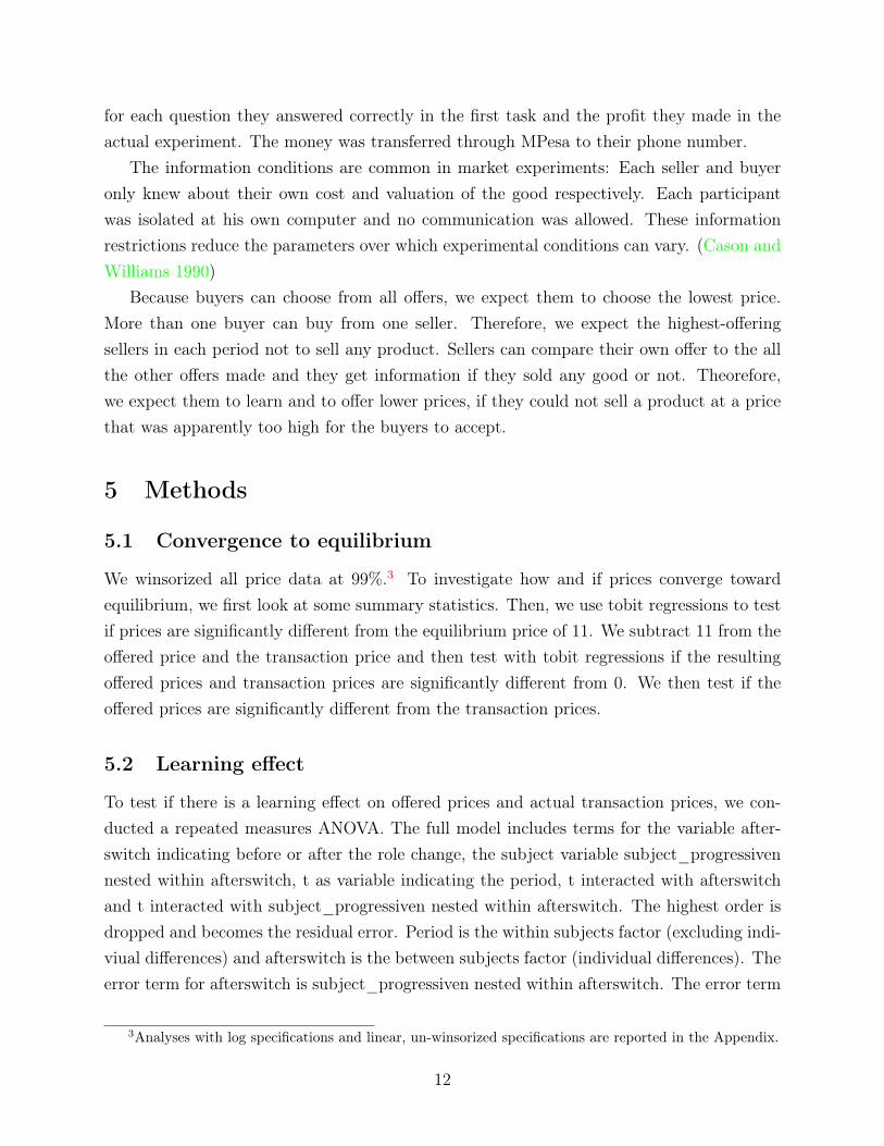
for each question they answered correctly in the first task and the profit they made in theactual experiment. The money was transferred through MPesa to their phone number.

The information conditions are common in market experiments: Each seller and buyeronly knew about their own cost and valuation of the good respectively. Each participantwas isolated at his own computer and no communication was allowed. These informationrestrictions reduce the parameters over which experimental conditions can vary. (Cason andWilliams 1990)

Because buyers can choose from all offers, we expect them to choose the lowest price.More than one buyer can buy from one seller. Therefore, we expect the highest-offeringsellers in each period not to sell any product. Sellers can compare their own offer to the allthe other offers made and they get information if they sold any good or not. Theorefore,we expect them to learn and to offer lower prices, if they could not sell a product at a pricethat was apparently too high for the buyers to accept.

5 Methods

5.1 Convergence to equilibrium

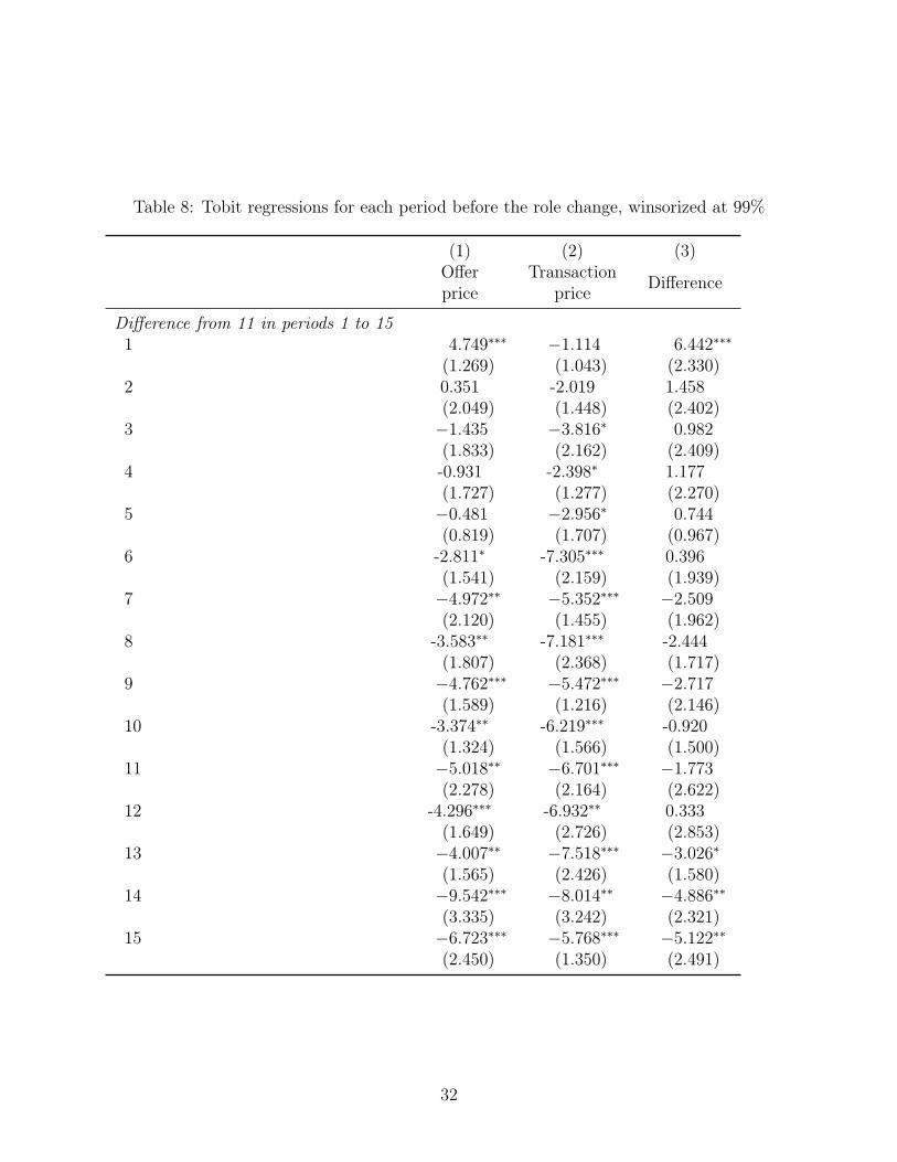
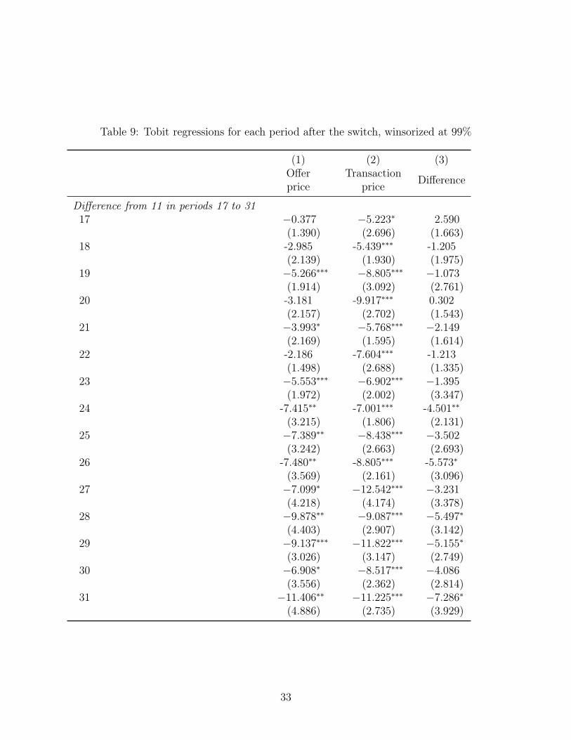
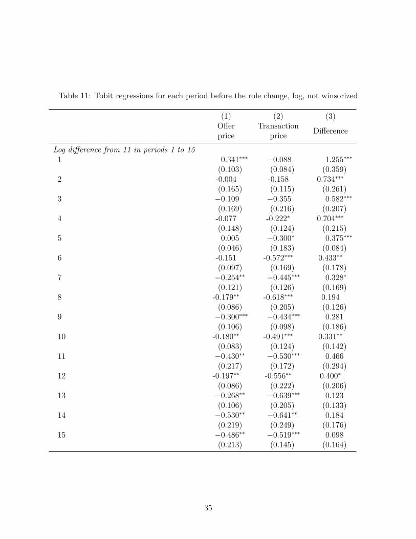
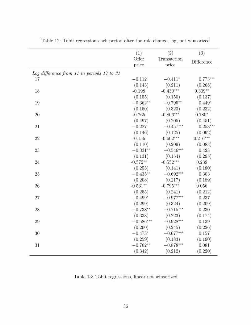
We winsorized all price data at 99%.3 To investigate how and if prices converge towardequilibrium, we first look at some summary statistics. Then, we use tobit regressions to testif prices are significantly different from the equilibrium price of 11. We subtract 11 from theoffered price and the transaction price and then test with tobit regressions if the resultingoffered prices and transaction prices are significantly different from 0. We then test if theoffered prices are significantly different from the transaction prices.

5.2 Learning effect

To test if there is a learning effect on offered prices and actual transaction prices, we con-ducted a repeated measures ANOVA. The full model includes terms for the variable after-switch indicating before or after the role change, the subject variable subject_progressivennested within afterswitch, t as variable indicating the period, t interacted with afterswitchand t interacted with subject_progressiven nested within afterswitch. The highest order isdropped and becomes the residual error. Period is the within subjects factor (excluding indi-viual differences) and afterswitch is the between subjects factor (individual differences). Theerror term for afterswitch is subject_progressiven nested within afterswitch. The error term

3Analyses with log specifications and linear, un-winsorized specifications are reported in the Appendix.

12

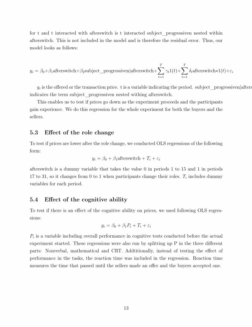
for t and t interacted with afterswitch is t interacted subject_progressiven nested withinafterswitch. This is not included in the model and is therefore the residual error. Thus, ourmodel looks as follows:

yi = β0+β1afterswitch+β2subject_progressiven|afterswitch+T∑t=1

γt1(t)+T∑t=1

δtafterswitch∗1(t)+εi

yi is the offered or the transaction price. t is a variable indicating the period. subject_progressiven|afterswitchindicates the term subject_progressiven nested withing afterswitch.

This enables us to test if prices go down as the experiment proceeds and the participantsgain experience. We do this regression for the whole experiment for both the buyers and thesellers.

5.3 Effect of the role change

To test if prices are lower after the role change, we conducted OLS regressions of the followingform:

yi = β0 + β1afterswitch+ Ti + εi

afterswitch is a dummy variable that takes the value 0 in periods 1 to 15 and 1 in periods17 to 31, so it changes from 0 to 1 when participants change their roles. Ti includes dummyvariables for each period.

5.4 Effect of the cognitive ability

To test if there is an effect of the cognitive ability on prices, we used following OLS regres-sions:

yi = β0 + β1Pi + Ti + εi

Pi is a variable including overall performance in cognitive tests conducted before the actualexperiment started. These regressions were also run by splitting up P in the three differentparts: Nonverbal, mathematical and CRT. Addtitionally, instead of testing the effect ofperformance in the tasks, the reaction time was included in the regression. Reaction timemeasures the time that passed until the sellers made an offer and the buyers accepted one.

13

6 Results

6.1 Convergence towards equilibrium

6.1.1 Summary statistics

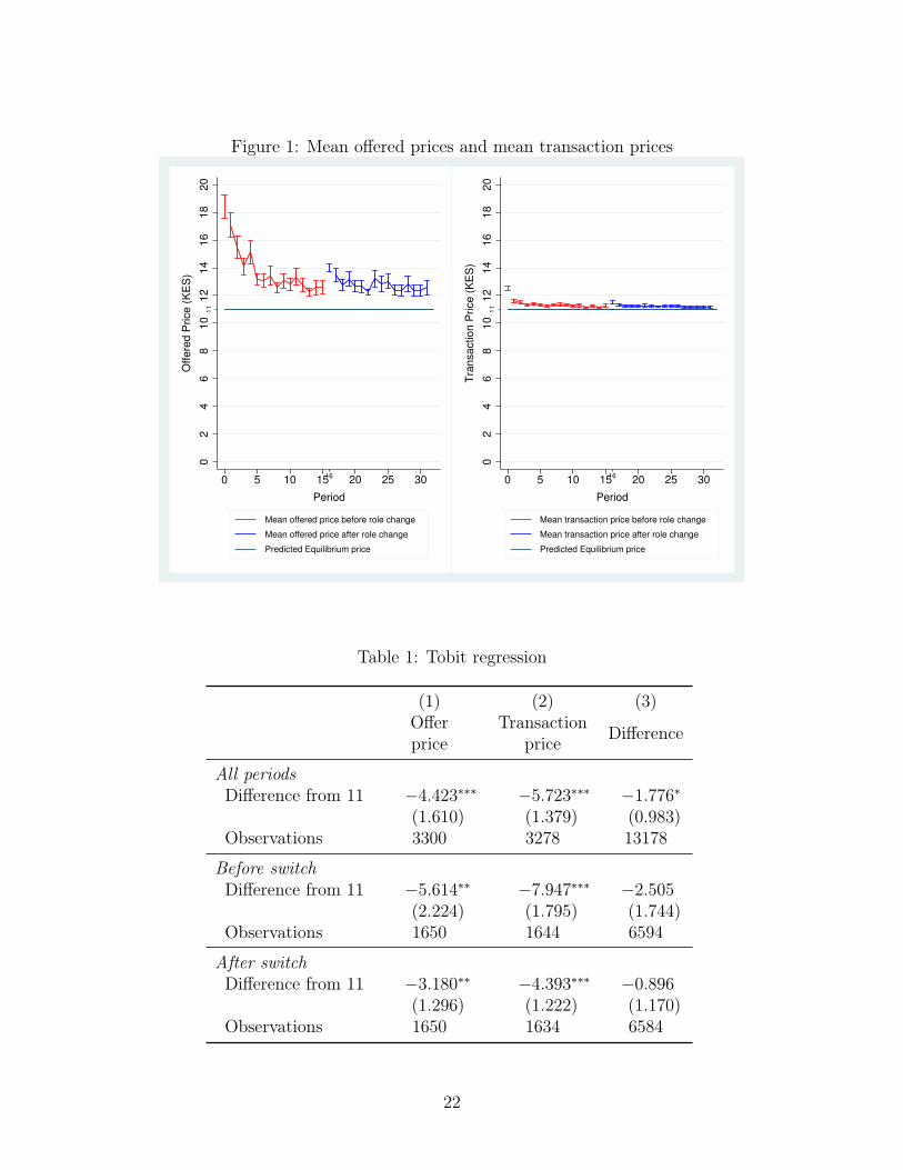
Figure 1 and 2 show the mean offered prices and the mean transaction prices, together withtheir standard errors, for each period. The mean offered prices start quite far above thetransaction prices and the predicted equilibrium price. They converge to a range between 12and 13 within 5 periods and stay there for the rest of the experiment. After the role change,the mean offered prices start much lower than in the first round, namely at around 13 andstayed again between 12 and 13 for the following periods. The standard errors are largestin the first four periods. The mean transaction prices are much lower than the mean offeredprice: They start below 12 and remain there until the end of the experiment. Buyers makefew and small mistakes: standard errors are much smaller than the ones of the offered prices.

So, we can conclude that mean offered prices start quite high above equilibrium but fallrelatively fast towards equilibrium, though they do not reach it. The small standard errorsshow that sellers make fewer and smaller mistakes as the experimnet proceeded. Becauseprices fall in the first periods and because they stayed low in later ones, there might be alearning effct. Additionally, the role change seems to have an effect on the price-setting be-havior of the sellers: Prices start from a lower level than in the first round of the experiment.The effect of experience is investigated below. Buyers make few and small mistakes: Pricesare near equilibrium and standard errors are much smaller than the ones of the offered prices.

6.1.2 Percentage of sellers and buyers at a certain price

Figures 4 and 5 show the percentage of sellers who offered a certain price and of buyers whoaccepted a certain price. The numbers of sellers who offered a price of 11 rises from 20%continuously to about 70%. After the switch, 45% of the sellers offer a price of 11, goingup to about 75%. The number of sellers who offer a price of 12 goes down from about 25%to 10% before the role change and from 20% to 5% afterwards. In the first period about60% of sellers offer a price of 13 or higher, going down to below 20%. After the switch,about 35% make an offer of 13 or higher, going down to 20%. Thus many sellers behave inaccordance with theory and offer a price of 11. Again, there seems to be a learning effect asthe experiment proceeds and an effect of the role change.

Buyers behave even more in accordance with theory. The amount of buyers who acceptea price of 11 rises from 65% to 90% before, and from 85% to 90%, sometimes 95% after theswitch. Initially, 20% of buyers accept a price of 12, going down to about 5%. After the

14

role change, not even 10% of buyers accept a price of 12, going down to less than 5%. Theamount of buyers who accept a price of 13 or higher starts from above 10% going down toabout 8% before the switch and is between 5% and 10% after the switch.

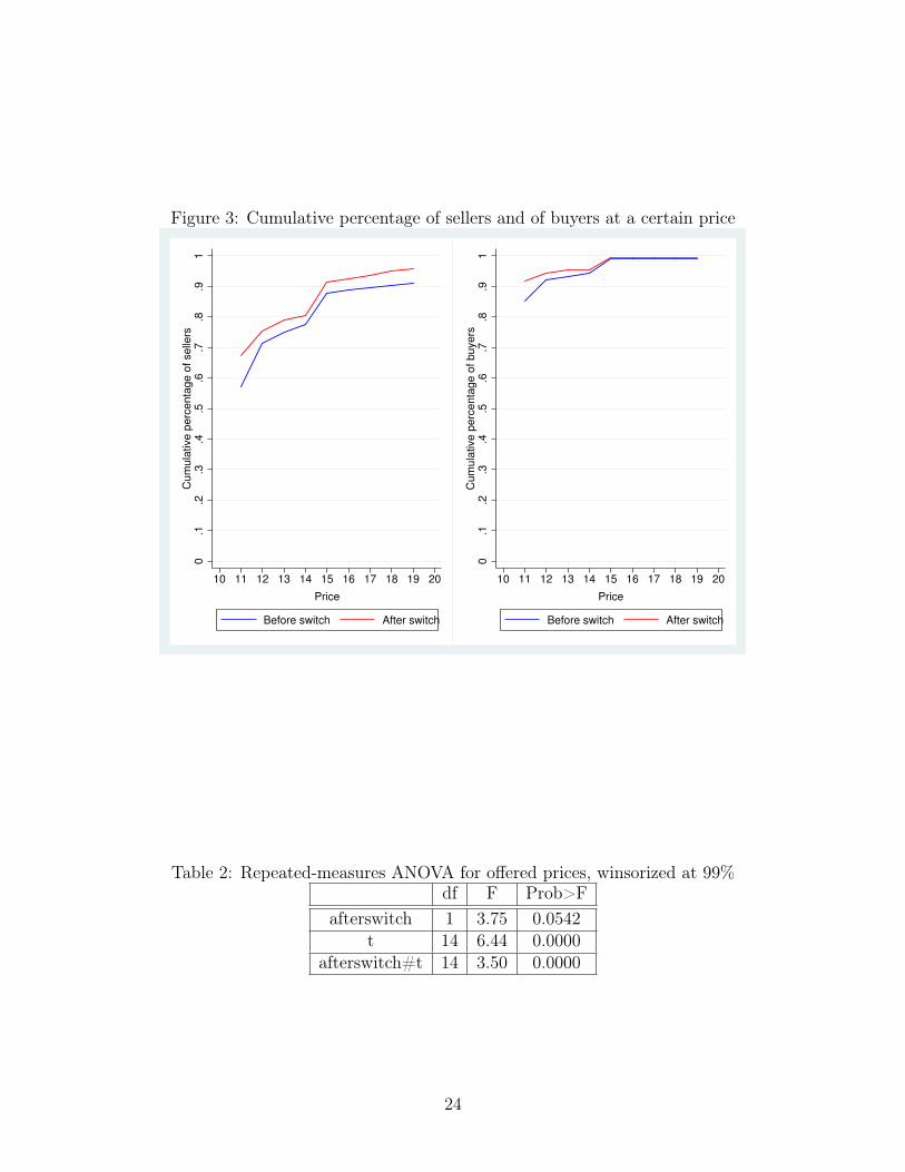
Figures 6 and 7 show the cumulative percentage of sellers and buyers at a certain priceboth before and after the role change. Cumulative percentages of sellers after the rolechange are consistently above the ones before the role change: Sellers seem to behave morein accordance with neoclassical price theory after the role change. The percentage of sellerswho offer a price of 20 KHS or higher falls from about 1% to about 0.5%. Also buyers seemto behave more correctly after the role change: Cumulative percentages are above the onesbefore the role change.

Together, these figures raise the question if there was a learning effect: People seem tobehave more in accordance with neoclassical price theory as the experiment proceeds andafter the role chance. Results of an ANOVA and of OLS regressions are reported below.

6.1.3 Tobit regressions

Table 1 shows tobit regressions to test if prices are significantly different from the predictedequilibrium price of 11 and if offered prices differed from transaction prices. The coefficientsare negative at the 1% to 5 % level. That means that people behave optimally: They wantto offer and to accept low prices. That prices are above 11 and do not completely reach 11lies in the fact that people can only make mistakes into one direction because they cannotoffer prices below 11.

6.2 Learning effect

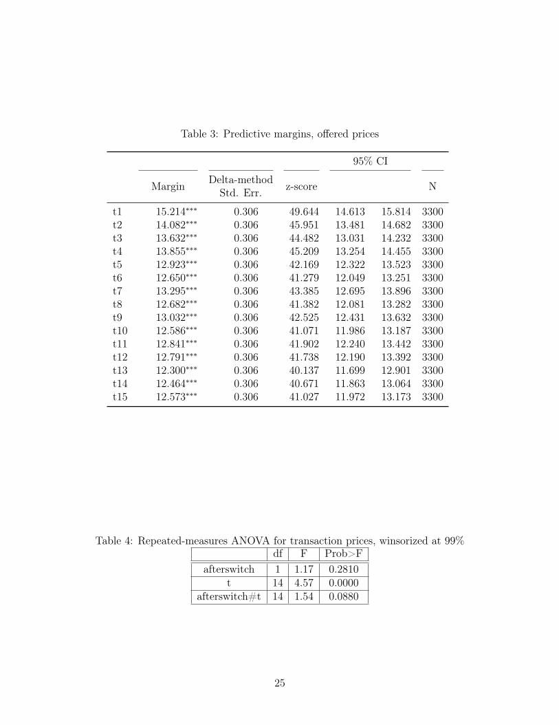
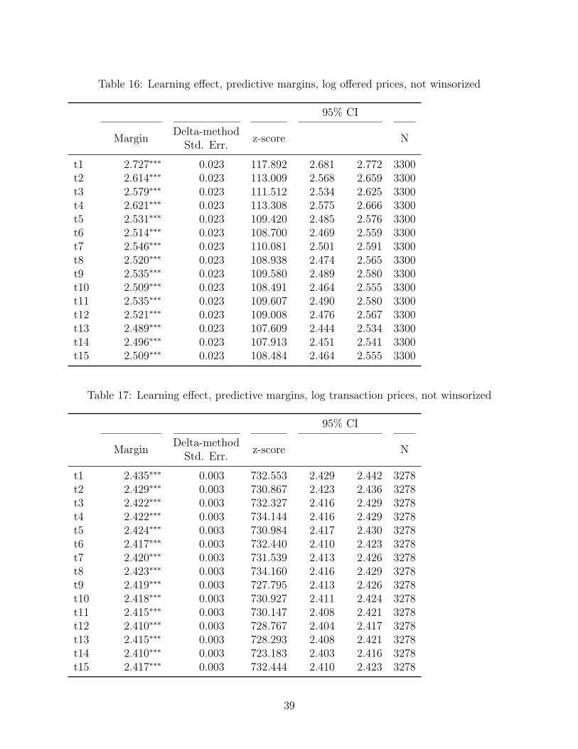
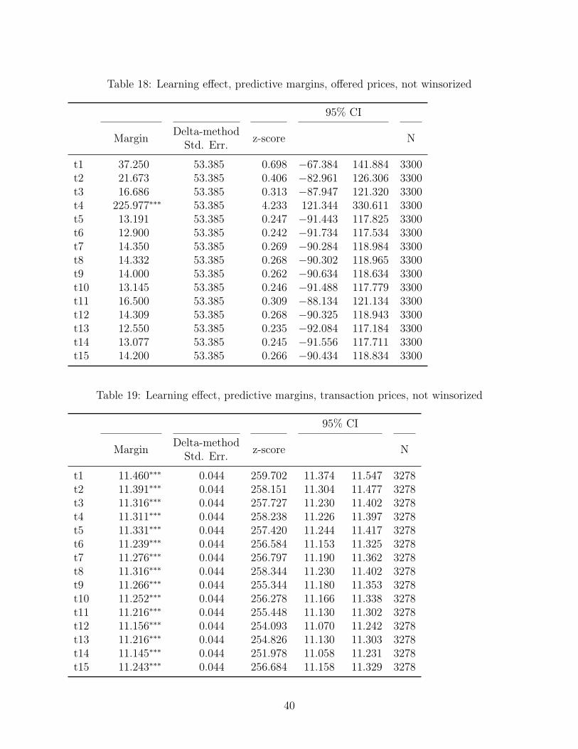
The results of the ANOVA which are presented in Table 2 show that there is a significanteffect of t on offered prices: The p-values of all three adjustments are equal or lower than0.01. Thus, prices change significantly over time. The R2 however is very small. Table 3shows the predictive margins: The mean offered prices fall continuously from 15.214 KESto 13.632 KES within three periods. The prices reach the lowest level of 12.300 KES in the13th period. After that, they rise again to 12.573 KES. The confidence intervalls for all butthe second period are lower than the confidence intervall for the first period. Though, someof the confidence intervalls overlap.

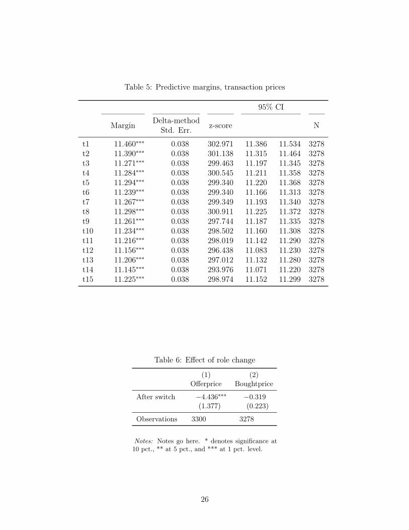
There is a significant effect of t on transaction prices as well which is showed in Table 4:the p-values of all three adjustments are below 0.01. The R2 is even smaller than for offeredprices, it is only 0.00777. The mean transaction prices decrease from 11.534 KES to 11.271KES within three periods. The lowest price of 11.145 KES is reached in the 14th period.

15

Some confidence intervalls overlap considerably. Again, the confidence intervalls for all butthe second period are lower than the confidence intervall for the first period.

So, there seems to be a learning effect on offered prices: There is a significant time effect,offered prices go down from 15.214 KES to 12.300 KES and all prices are significantly lowerthan the first one (with the exception of the price in the second period). But prices donot drop continuously. There is a significant learning effect on transaction prices as well,though again prices do not drop continuously and the effect is smaller than on offered prices:Transaction prices go down from 11.534 KES to 11.145 KES.

6.3 Effect of role change

Table 3 shows the results of the OLS regression to test if there is an effect of the role changeon the offered and the transaction prices. There is a significant effect of the role change onoffered prices at the 1% level: Everything else being held constant, the role change lowersthe offered prices by 4.436 KHS. There is no effect on the transaction prices.

Because offered prices are lower after the role change, we can conlcude that market expe-rience indeed plays an important role: Sellers behave more in accordance with neoclassicalmarket theory if they gained market experience as buyers before. Buyers do not changebehavior after the role change.

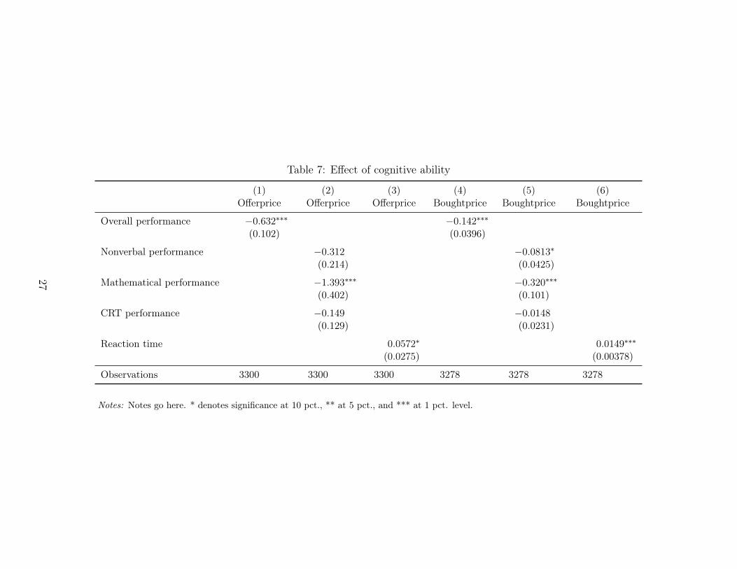
6.4 Effect of cognitive ability

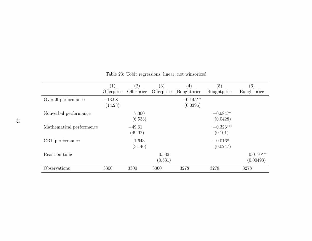
Table 4 shows the effects of cognitive ability on offered and transaction prices. Cognitiveability is measured as performance in test questions that were asked before the experimentand in reaction time of buyers and sellers to make an offer or accept one. Everything elsebeing held constant, there is a significant negative effect of overall performance in the pre-experiment questions on both offered and transaction prices on the 1% level. By lookingat the performance in the individual tasks, we only find a significant negative effect ofmathematical performace on offered prices. There is a significant effect of nonverbal andmathematical performance on transaction prices.

Thus, if people are more intelligent, they behave more in accordance with neoclassicalprice theory: They offer and accept lower prices. There is a significant positive effect ofreaction time on offered and transaction prices: If more time passed until an offer wasmade or accepted, prices were higher. That supports our finding that people who are moreintelligent behave more correctly.

16

7 Conclusion

The aim of this paper was to investigate the predictions of neoclassical price theory in theNairobi informal settlement of Kibera in Kenya. For this purpose, the investigation wasmoved back to the laboratory and an experiment similar to posted-offer market experiments4was conducted.

Smith (e.g. Smith 1962) and many researchers after him show that we can understandmarket mechanisms by conducting experiements in laboratories. Predicted outcomes of neo-classical price theory hold in experimental laboratory settings, also in posted-offer marketssettings. The experiment presented in this paper was conducted in Kenya and examines amarket structure similar to a posted-offer market. From earlier findings, we might expectthe predictions of neoclassical price theory to hold in our experimental setting. However,there are doubts if people from different countries and cultural backgrounds are comparableto WEIRD (Western, Educated, Industrialized, Rich, and Democratic) people, who are themost common participants in lab experiments. In particular, there is evidence from one fieldexperiment in Sierra Leona that equilibrium is not reached. So, it might be the case thatneoclassical price theory does not hold for the experiment conducted in Kenya.

We investigated convergence to market equilibrium and the presence of a learning effectas the experiment proceeds, both for buyers and sellers. In addition, we tested if cognitiveability has an effect on the prices offered and on the actual transaction prices.

Our salient finding shows that participants of the experiment behave near-optimally:sellers offer, and buyers buy at, prices near the theoretically predicted equilibrium. Thatprices are above 11 and do not completely reach 11 lies in the fact that people can onlymake mistakes into one direction because they cannot offer prices below 11. There is asignificant effect of the periods on offered and transaction prices. Though, mean prices donot drop continuously. The effect on transaction prices is smaller than on offered prices.Market experience does play an important role on sellers: Offered prices are lower afterthe role change. So, sellers behave correctly but they learn as the experiment proceedsand offer significantly lower prices after having gained market experience as buyers. Buyersseem to behave even more in accordance with market theory: They only accept prices nearequilibrium from the beginning. The strength of the learning effect is small and transactionprices are not significantly lower after the role change. If people are more intelligent, theybehave more in accordance with neoclassical price theory: They offer and accept lower prices.

So, like in earlier findings from posted-offer market experiments, prices converge towards

4Literature about posted-offer market experiments: (Davis and Holt 1993; Davis and Williams 1986;Ketcham et al. 1984; Plott and Smith 1978; Smith and Williams 2000; Williams 1973)

17

equilibrium and market experience has a significant negative effect on prices. Earlier findingshowever showed that convergence in posted-offer market experiments is not complete. In theexperiment reported in this paper, this inefficiency can be explained through the fact thatpeople can only make mistakes into one direction. People actually behave optimally: Theyboth want to offer and to accept low prices.

Our findings contradict Bulte et al. (2012): the experiment reported in this paper showsthat a market consisting of informal settlement inhabitants does work: Participants behaveoptimally and prices converge toward equilibrium. There is evidence that basic marketmechanisms do work in developing countries. Thus, the failure of basic market mechanismsis unlikely to be the cause for market failures in developing countries. If this result is robustin other settings remains to be investigated.

Markets have been investigated in laboratory experiments in the western world a lot oftimes and helped to understand basic market mechanisms. This paper delivers evidencethat we can investigate market mechanisms in developing countries in the laboratory aswell, which provides the opportunity to investigate different market structures and gettingto understand markets in developing countries.

18

8 References

References

Bulte, E., A. Kontoleon, J. List, T. Turley, and M. Voors (2012). When economics meetshierarchy: A field experiment on the workings of the invisible hand. Working paper.

Cardenas, J. C. and J. Carpenter (2004, October). Experimental development economics:A review of the literature and ideas for future research. Technical report.

Cardenas, J. C. and J. Carpenter (2008). Behavioural development economics: Lessonsfrom field labs in the developing world. The Journal of Development Studies 44 (3),311–338.

Cason, T. N. and A. W. Williams (1990, December). Competitive equilibrium conver-gence in a posted-offer market with extreme earnings inequities. Journal of EconomicBehavior & Organization 14 (3), 331–352.

Chamberlin, E. H. (1948, April). An experimental imperfect market. Journal of PoliticalEconomy 56 (2), 95–108. ArticleType: research-article / Full publication date: Apr.,1948 / Copyright c© 1948 The University of Chicago Press.

Davis, D. D. and C. A. Holt (1993). Experimental Economics. Princeton, New Jersey:Princeton University Press.

Davis, D. D. and A. W. Williams (1986, September). The effects of rent asymmetries inposted offer markets. Journal of Economic Behavior & Organization 7 (3), 303–316.

Haushofer, J., M. Collins, D. Giusti, Giovanna, J. M. Njoroge, A. Odero, and C. Onyango(2012, October). The busara center: A laboratory environment for developing coun-tries. SSRN Scholarly Paper ID 2155217, Social Science Research Network, Rochester,NY.

Henrich, J., R. Boyd, R. McElreath, M. Gurven, P. J. Richerson, J. Ensminger, M. Alvard,A. Barr, C. Barrett, A. Bolyanatz, C. F. Camerer, J.-C. Cardenas, E. Fehr, H. M.Gintis, F. Gil-White, E. L. Gwako, N. Henrich, K. Hill, C. Lesorogol, J. Q. Patton,F. W. Marlowe, D. P. Tracer, and J. Ziker (2012, October). Culture does account forvariation in game behavior. Proceedings of the National Academy of Sciences 109 (2),E32–E33. PMID: 22219355.

Henrich, J., J. Ensminger, R. McElreath, A. Barr, C. Barrett, A. Bolyanatz, J. C. Car-denas, M. Gurven, E. Gwako, N. Henrich, C. Lesorogol, F. Marlowe, D. Tracer, and

19

J. Ziker (2010, March). Markets, religion, community size, and the evolution of fairnessand punishment. Science 327 (5972), 1480–1484. PMID: 20299588.

Henrich, J., S. J. Heine, and A. Norenzayan (2010a, July). Most people are not WEIRD.Nature 466 (7302), 29–29.

Henrich, J., S. J. Heine, and A. Norenzayan (2010b, June). The weirdest people in theworld? The Behavioral and brain sciences 33 (2-3), 61–83; discussion 83–135. PMID:20550733.

Henrich, J., R. McElreath, A. Barr, J. Ensminger, C. Barrett, A. Bolyanatz, J. C. Car-denas, M. Gurven, E. Gwako, N. Henrich, C. Lesorogol, F. Marlowe, D. Tracer, andJ. Ziker (2006, June). Costly punishment across human societies. Science 312 (5781),1767–1770. PMID: 16794075.

Ketcham, J., V. L. Smith, and A. W. Williams (1984, October). A comparison of posted-offer and double-auction pricing institutions. The Review of Economic Studies 51 (4),595–614.

List, J. A. (2002, November). Testing neoclassical competitive market theory in thefield. Proceedings of the National Academy of Sciences 99 (24), 15827–15830. PMID:12432103.

List, J. A. (2004). Testing neoclassical competitive theory in multilateral decentralizedmarkets. Journal of Political Economy 112 (5), 1131–1156.

Plott, C. R. and V. L. Smith (1978, February). An experimental examination of twoexchange institutions. The Review of Economic Studies 45 (1), 133–153.

Smith, V. L. (1962, January). An experimental study of competitive market behavior.Journal of Political Economy 70 (2), 111–137.

Smith, V. L. (1964, May). Effect of market organization on competitive equilibrium. TheQuarterly Journal of Economics 78 (2), 181–201.

Smith, V. L. (1965, January). Experimental auction markets and the walrasian hypothesis.Journal of Political Economy 73 (4), 387–393.

Smith, V. L. (1976, May). Experimental economics: Induced value theory. The AmericanEconomic Review 66 (2), 274–279. ArticleType: research-article / Issue Title: Papersand Proceedings of the Eighty-eighth Annual Meeting of the American Economic As-sociation / Full publication date: May, 1976 / Copyright c© 1976 American EconomicAssociation.

20

Smith, V. L. and A. W. Williams (1982, March). The effects of rent asymmetries inexperimental auction markets. Journal of Economic Behavior & Organization 3 (1),99–116.

Smith, V. L. and A. W. Williams (2000). The boundaries of competitive price theory:Convergence, expectations, and transaction costs. In V. L. Smith (Ed.), Bargainingand Market Behavior : Essays in Experimental Economics, pp. 286–319. Cambridge,UK; New York: Cambridge University Press.

Walker, J. M. and A. W. Williams (1988). Market behavior in bid, offer, and doubleauctions: A reexmination. Journal of Economic Behavior & Organization 9 (3), 301–314.

Williams, F. E. (1973, January). The effect of market organization on competitive equi-librium: the multi-unit case. The Review of Economic Studies 40 (1), 97–113. Article-Type: research-article / Full publication date: Jan., 1973 / Copyright c© 1973 TheReview of Economic Studies, Ltd.

21

Figure 1: Mean offered prices and mean transaction prices

11

02

46

810

12

14

16

18

20

Offere

d P

rice (

KE

S)

160 5 10 15 20 25 30

Period

Mean offered price before role change

Mean offered price after role change

Predicted Equilibrium price

11

02

46

810

12

14

16

18

20

Tra

nsaction P

rice (

KE

S)

160 5 10 15 20 25 30

Period

Mean transaction price before role change

Mean transaction price after role change

Predicted Equilibrium price

Table 1: Tobit regression

(1) (2) (3)Offerprice

Transactionprice Difference

All periodsDifference from 11 −4.423∗∗∗ −5.723∗∗∗ −1.776∗

(1.610) (1.379) (0.983)Observations 3300 3278 13178

Before switchDifference from 11 −5.614∗∗ −7.947∗∗∗ −2.505

(2.224) (1.795) (1.744)Observations 1650 1644 6594

After switchDifference from 11 −3.180∗∗ −4.393∗∗∗ −0.896

(1.296) (1.222) (1.170)Observations 1650 1634 6584

22

Figure 2: Percentage of sellers and of buyers at a certain price

23

Figure 3: Cumulative percentage of sellers and of buyers at a certain price0

.1.2

.3.4

.5.6

.7.8

.91

Cum

ula

tive p

erc

enta

ge o

f selle

rs

10 11 12 13 14 15 16 17 18 19 20

Price

Before switch After switch

0.1

.2.3

.4.5

.6.7

.8.9

1C

um

ula

tive p

erc

enta

ge o

f buyers

10 11 12 13 14 15 16 17 18 19 20

Price

Before switch After switch

Table 2: Repeated-measures ANOVA for offered prices, winsorized at 99%df F Prob>F

afterswitch 1 3.75 0.0542t 14 6.44 0.0000

afterswitch#t 14 3.50 0.0000

24

Table 3: Predictive margins, offered prices

95% CI

Margin Delta-methodStd. Err. z-score N

t1 15.214∗∗∗ 0.306 49.644 14.613 15.814 3300t2 14.082∗∗∗ 0.306 45.951 13.481 14.682 3300t3 13.632∗∗∗ 0.306 44.482 13.031 14.232 3300t4 13.855∗∗∗ 0.306 45.209 13.254 14.455 3300t5 12.923∗∗∗ 0.306 42.169 12.322 13.523 3300t6 12.650∗∗∗ 0.306 41.279 12.049 13.251 3300t7 13.295∗∗∗ 0.306 43.385 12.695 13.896 3300t8 12.682∗∗∗ 0.306 41.382 12.081 13.282 3300t9 13.032∗∗∗ 0.306 42.525 12.431 13.632 3300t10 12.586∗∗∗ 0.306 41.071 11.986 13.187 3300t11 12.841∗∗∗ 0.306 41.902 12.240 13.442 3300t12 12.791∗∗∗ 0.306 41.738 12.190 13.392 3300t13 12.300∗∗∗ 0.306 40.137 11.699 12.901 3300t14 12.464∗∗∗ 0.306 40.671 11.863 13.064 3300t15 12.573∗∗∗ 0.306 41.027 11.972 13.173 3300

Table 4: Repeated-measures ANOVA for transaction prices, winsorized at 99%df F Prob>F

afterswitch 1 1.17 0.2810t 14 4.57 0.0000

afterswitch#t 14 1.54 0.0880

25

Table 5: Predictive margins, transaction prices

95% CI

Margin Delta-methodStd. Err. z-score N

t1 11.460∗∗∗ 0.038 302.971 11.386 11.534 3278t2 11.390∗∗∗ 0.038 301.138 11.315 11.464 3278t3 11.271∗∗∗ 0.038 299.463 11.197 11.345 3278t4 11.284∗∗∗ 0.038 300.545 11.211 11.358 3278t5 11.294∗∗∗ 0.038 299.340 11.220 11.368 3278t6 11.239∗∗∗ 0.038 299.340 11.166 11.313 3278t7 11.267∗∗∗ 0.038 299.349 11.193 11.340 3278t8 11.298∗∗∗ 0.038 300.911 11.225 11.372 3278t9 11.261∗∗∗ 0.038 297.744 11.187 11.335 3278t10 11.234∗∗∗ 0.038 298.502 11.160 11.308 3278t11 11.216∗∗∗ 0.038 298.019 11.142 11.290 3278t12 11.156∗∗∗ 0.038 296.438 11.083 11.230 3278t13 11.206∗∗∗ 0.038 297.012 11.132 11.280 3278t14 11.145∗∗∗ 0.038 293.976 11.071 11.220 3278t15 11.225∗∗∗ 0.038 298.974 11.152 11.299 3278

Table 6: Effect of role change

(1) (2)Offerprice Boughtprice

After switch −4.436∗∗∗ −0.319(1.377) (0.223)

Observations 3300 3278

Notes: Notes go here. * denotes significance at10 pct., ** at 5 pct., and *** at 1 pct. level.

26

Table 7: Effect of cognitive ability

(1) (2) (3) (4) (5) (6)Offerprice Offerprice Offerprice Boughtprice Boughtprice Boughtprice

Overall performance −0.632∗∗∗ −0.142∗∗∗(0.102) (0.0396)

Nonverbal performance −0.312 −0.0813∗(0.214) (0.0425)

Mathematical performance −1.393∗∗∗ −0.320∗∗∗(0.402) (0.101)

CRT performance −0.149 −0.0148(0.129) (0.0231)

Reaction time 0.0572∗ 0.0149∗∗∗

(0.0275) (0.00378)

Observations 3300 3300 3300 3278 3278 3278

Notes: Notes go here. * denotes significance at 10 pct., ** at 5 pct., and *** at 1 pct. level.

27

Figure 4: Log mean offered and transaction prices, not winsorized

0.5

11.5

22.5

33.5

lnofferp

rice (

KE

S)

0 10 20 30

Period

Mean lnofferprice before role change

Mean lnofferprice after role change

Log predicted equilibrium price

0.5

11.5

22.5

33.5

lnboughtp

rice (

KE

S)

0 10 20 30

Period

Mean lnboughtprice before role change

Mean lnboughtprice after role change

Log predicted equilibrium price

9 Appendix

28

Figure 5: Mean offered and transaction prices, linear, not winsorized

11

0200

400

600

800

1000

Offere

d P

rice (

KE

S)

160 10 20 30

Period

Mean offered price before role change

Mean offered price after role change

Predicted Equilibrium price

11

0200

400

600

800

1000

Tra

nsaction P

rice (

KE

S)

160 10 20 30

Period

Mean transaction price before role change

Mean transaction price after role change

Predicted Equilibrium price

29

Figure 6: Percentage of sellers and of buyers at a certain price, linear, not winsorized

30

Figure 7: Cumulative percentage of sellers and of buyers at a certain price, linear, notwinsorized

0.1

.2.3

.4.5

.6.7

.8.9

1C

um

ula

tive p

erc

enta

ge o

f selle

rs

10 11 12 13 14 15 16 17 18 19 20

Price

Before switch After switch

0.1

.2.3

.4.5

.6.7

.8.9

1C

um

ula

tive p

erc

enta

ge o

f buyers

10 11 12 13 14 15 16 17 18 19 20

Price

Before switch After switch

31

Table 8: Tobit regressions for each period before the role change, winsorized at 99%

(1) (2) (3)Offerprice

Transactionprice Difference

Difference from 11 in periods 1 to 151 4.749∗∗∗ −1.114 6.442∗∗∗

(1.269) (1.043) (2.330)2 0.351 -2.019 1.458

(2.049) (1.448) (2.402)3 −1.435 −3.816∗ 0.982

(1.833) (2.162) (2.409)4 -0.931 -2.398∗ 1.177

(1.727) (1.277) (2.270)5 −0.481 −2.956∗ 0.744

(0.819) (1.707) (0.967)6 -2.811∗ -7.305∗∗∗ 0.396

(1.541) (2.159) (1.939)7 −4.972∗∗ −5.352∗∗∗ −2.509

(2.120) (1.455) (1.962)8 -3.583∗∗ -7.181∗∗∗ -2.444

(1.807) (2.368) (1.717)9 −4.762∗∗∗ −5.472∗∗∗ −2.717

(1.589) (1.216) (2.146)10 -3.374∗∗ -6.219∗∗∗ -0.920

(1.324) (1.566) (1.500)11 −5.018∗∗ −6.701∗∗∗ −1.773

(2.278) (2.164) (2.622)12 -4.296∗∗∗ -6.932∗∗ 0.333

(1.649) (2.726) (2.853)13 −4.007∗∗ −7.518∗∗∗ −3.026∗

(1.565) (2.426) (1.580)14 −9.542∗∗∗ −8.014∗∗ −4.886∗∗

(3.335) (3.242) (2.321)15 −6.723∗∗∗ −5.768∗∗∗ −5.122∗∗

(2.450) (1.350) (2.491)

32

Table 9: Tobit regressions for each period after the switch, winsorized at 99%

(1) (2) (3)Offerprice

Transactionprice Difference

Difference from 11 in periods 17 to 3117 −0.377 −5.223∗ 2.590

(1.390) (2.696) (1.663)18 -2.985 -5.439∗∗∗ -1.205

(2.139) (1.930) (1.975)19 −5.266∗∗∗ −8.805∗∗∗ −1.073

(1.914) (3.092) (2.761)20 -3.181 -9.917∗∗∗ 0.302

(2.157) (2.702) (1.543)21 −3.993∗ −5.768∗∗∗ −2.149

(2.169) (1.595) (1.614)22 -2.186 -7.604∗∗∗ -1.213

(1.498) (2.688) (1.335)23 −5.553∗∗∗ −6.902∗∗∗ −1.395

(1.972) (2.002) (3.347)24 -7.415∗∗ -7.001∗∗∗ -4.501∗∗

(3.215) (1.806) (2.131)25 −7.389∗∗ −8.438∗∗∗ −3.502

(3.242) (2.663) (2.693)26 -7.480∗∗ -8.805∗∗∗ -5.573∗

(3.569) (2.161) (3.096)27 −7.099∗ −12.542∗∗∗ −3.231

(4.218) (4.174) (3.378)28 −9.878∗∗ −9.087∗∗∗ −5.497∗

(4.403) (2.907) (3.142)29 −9.137∗∗∗ −11.822∗∗∗ −5.155∗

(3.026) (3.147) (2.749)30 −6.908∗ −8.517∗∗∗ −4.086

(3.556) (2.362) (2.814)31 −11.406∗∗ −11.225∗∗∗ −7.286∗

(4.886) (2.735) (3.929)

33

Table 10: Tobit regressions, log, not winsorized

(1) (2) (3)Offerprice

Transactionprice Difference

All periodsLog difference from 11 −0.340∗∗ −0.475∗∗∗ 0.375∗∗∗

(0.138) (0.120) (0.079)Observations 3300 3278 6579

Before switchLog difference from 11 −0.473∗∗ −0.643∗∗∗ 0.310∗∗

(0.215) (0.146) (0.137)Observations 1650 1644 3294

After switchLog difference from 11 −0.227∗∗ −0.371∗∗∗ 0.443∗∗∗

(0.108) (0.112) (0.116)Observations 1650 1634 3285

34

Table 11: Tobit regressions for each period before the role change, log, not winsorized

(1) (2) (3)Offerprice

Transactionprice Difference

Log difference from 11 in periods 1 to 151 0.341∗∗∗ −0.088 1.255∗∗∗

(0.103) (0.084) (0.359)2 -0.004 -0.158 0.734∗∗∗

(0.165) (0.115) (0.261)3 −0.109 −0.355 0.582∗∗∗

(0.169) (0.216) (0.207)4 -0.077 -0.222∗ 0.704∗∗∗

(0.148) (0.124) (0.215)5 0.005 −0.300∗ 0.375∗∗∗

(0.046) (0.183) (0.084)6 -0.151 -0.572∗∗∗ 0.433∗∗

(0.097) (0.169) (0.178)7 −0.254∗∗ −0.445∗∗∗ 0.328∗

(0.121) (0.126) (0.169)8 -0.179∗∗ -0.618∗∗∗ 0.194

(0.086) (0.205) (0.126)9 −0.300∗∗∗ −0.434∗∗∗ 0.281

(0.106) (0.098) (0.186)10 -0.180∗∗ -0.491∗∗∗ 0.331∗∗

(0.083) (0.124) (0.142)11 −0.430∗∗ −0.530∗∗∗ 0.466

(0.217) (0.172) (0.294)12 -0.197∗∗ -0.556∗∗ 0.400∗

(0.086) (0.222) (0.206)13 −0.268∗∗ −0.639∗∗∗ 0.123

(0.106) (0.205) (0.133)14 −0.530∗∗ −0.641∗∗ 0.184

(0.219) (0.249) (0.176)15 −0.486∗∗ −0.519∗∗∗ 0.098

(0.213) (0.145) (0.164)

35

Table 12: Tobit regressionseach period after the role change, log, not winsorized

(1) (2) (3)Offerprice

Transactionprice Difference

Log difference from 11 in periods 17 to 3117 −0.112 −0.411∗ 0.773∗∗∗

(0.143) (0.211) (0.268)18 -0.198 -0.430∗∗∗ 0.309∗∗

(0.155) (0.150) (0.137)19 −0.362∗∗ −0.795∗∗ 0.449∗

(0.150) (0.323) (0.232)20 -0.765 -0.806∗∗∗ 0.780∗

(0.497) (0.205) (0.451)21 −0.227 −0.457∗∗∗ 0.253∗∗∗

(0.146) (0.125) (0.092)22 -0.156 -0.602∗∗∗ 0.216∗∗∗

(0.110) (0.209) (0.083)23 −0.331∗∗ −0.546∗∗∗ 0.428

(0.131) (0.154) (0.295)24 -0.572∗∗ -0.552∗∗∗ 0.239

(0.255) (0.141) (0.180)25 −0.435∗∗ −0.692∗∗∗ 0.303

(0.208) (0.217) (0.189)26 -0.531∗∗ -0.795∗∗∗ 0.056

(0.255) (0.241) (0.212)27 −0.499∗ −0.977∗∗∗ 0.237

(0.299) (0.324) (0.209)28 −0.738∗∗ −0.715∗∗∗ 0.230

(0.338) (0.223) (0.174)29 −0.586∗∗∗ −0.928∗∗∗ 0.139

(0.200) (0.245) (0.226)30 −0.473∗ −0.677∗∗∗ 0.157

(0.259) (0.183) (0.190)31 −0.762∗∗ −0.878∗∗∗ 0.081

(0.342) (0.212) (0.220)

Table 13: Tobit regressions, linear not winsorized

36

Table 14: Tobit regressions before the role change, linear, not winsorized

(1) (2) (3)Offerprice

Transactionprice Difference

Difference from 11 in periods 1 to 151 6.849 −1.114 27.440

(12.136) (1.043) (31.909)2 -56.681 -2.019 -37.730

(38.061) (1.448) (30.649)3 −26.750 −4.704 −9.971

(19.463) (2.910) (14.020)4 -44.018 -2.950∗ -22.720

(28.334) (1.677) (20.258)5 −0.671 −4.122 0.498

(0.915) (2.546) (1.007)6 -6.380∗ -7.305∗∗∗ -0.428

(3.471) (2.159) (2.909)7 −9.773∗∗ −5.730∗∗∗ −4.987∗

(4.214) (1.630) (2.997)8 -4.017∗ -8.158∗∗∗ -2.825

(2.082) (2.753) (1.852)9 −12.625∗∗∗ −5.472∗∗∗ −7.004

(4.153) (1.216) (4.321)10 -6.703∗∗ -6.219∗∗∗ -2.236

(3.151) (1.566) (2.381)11 −63.689∗ −6.701∗∗∗ −29.247

(34.574) (2.164) (21.904)12 -5.203∗∗∗ -6.932∗∗ 0.212

(1.921) (2.726) (3.227)13 −4.007∗∗ −8.214∗∗∗ −3.141∗

(1.565) (2.671) (1.627)14 −16.976∗ −8.014∗∗ −8.679

(8.901) (3.242) (5.586)15 −32.558∗ −6.870∗∗∗ −22.878∗

(17.218) (2.090) (12.981)

37

Table 15: Tobit regressions after the role change, linear, not winsorized

(1) (2) (3)Offerprice

Transactionprice Difference

Difference from 11 in periods 17 to 3117 −97.708∗∗ −5.223∗ 8.237

(48.498) (2.696) (46.629)18 -9.791 -5.439∗∗∗ -4.560

(6.204) (1.930) (4.434)19 −26.248∗∗ −10.641∗∗ −9.054

(12.323) (4.557) (9.308)20 -4580.201∗ -10.406∗∗∗ -1025.794

(2644.529) (2.623) (1060.291)21 −8.695 −5.768∗∗∗ −4.627

(5.697) (1.595) (3.524)22 -2.186 -7.604∗∗∗ -1.213

(1.498) (2.688) (1.335)23 −14.383∗∗∗ −6.902∗∗∗ −4.570

(4.518) (2.002) (6.557)24 -36.912∗∗ -7.001∗∗∗ -21.036∗∗

(17.555) (1.806) (9.932)25 −16.512∗∗ −8.857∗∗∗ −7.980

(8.284) (2.796) (4.996)26 -20.639∗ -10.641∗∗∗ -14.129∗

(11.809) (3.474) (8.376)27 −19.609 −12.542∗∗∗ −8.766

(12.781) (4.174) (8.028)28 −44.417∗ −9.087∗∗∗ −23.854∗

(22.979) (2.907) (13.649)29 −18.845∗∗ −11.822∗∗∗ −10.182∗∗

(7.727) (3.147) (4.428)30 −19.033 −8.517∗∗∗ −10.746

(11.592) (2.362) (7.334)31 −30.683∗∗ −11.225∗∗∗ −18.288∗

(14.683) (2.735) (10.677)

38

Table 16: Learning effect, predictive margins, log offered prices, not winsorized

95% CI

Margin Delta-methodStd. Err. z-score N

t1 2.727∗∗∗ 0.023 117.892 2.681 2.772 3300t2 2.614∗∗∗ 0.023 113.009 2.568 2.659 3300t3 2.579∗∗∗ 0.023 111.512 2.534 2.625 3300t4 2.621∗∗∗ 0.023 113.308 2.575 2.666 3300t5 2.531∗∗∗ 0.023 109.420 2.485 2.576 3300t6 2.514∗∗∗ 0.023 108.700 2.469 2.559 3300t7 2.546∗∗∗ 0.023 110.081 2.501 2.591 3300t8 2.520∗∗∗ 0.023 108.938 2.474 2.565 3300t9 2.535∗∗∗ 0.023 109.580 2.489 2.580 3300t10 2.509∗∗∗ 0.023 108.491 2.464 2.555 3300t11 2.535∗∗∗ 0.023 109.607 2.490 2.580 3300t12 2.521∗∗∗ 0.023 109.008 2.476 2.567 3300t13 2.489∗∗∗ 0.023 107.609 2.444 2.534 3300t14 2.496∗∗∗ 0.023 107.913 2.451 2.541 3300t15 2.509∗∗∗ 0.023 108.484 2.464 2.555 3300

Table 17: Learning effect, predictive margins, log transaction prices, not winsorized

95% CI

Margin Delta-methodStd. Err. z-score N

t1 2.435∗∗∗ 0.003 732.553 2.429 2.442 3278t2 2.429∗∗∗ 0.003 730.867 2.423 2.436 3278t3 2.422∗∗∗ 0.003 732.327 2.416 2.429 3278t4 2.422∗∗∗ 0.003 734.144 2.416 2.429 3278t5 2.424∗∗∗ 0.003 730.984 2.417 2.430 3278t6 2.417∗∗∗ 0.003 732.440 2.410 2.423 3278t7 2.420∗∗∗ 0.003 731.539 2.413 2.426 3278t8 2.423∗∗∗ 0.003 734.160 2.416 2.429 3278t9 2.419∗∗∗ 0.003 727.795 2.413 2.426 3278t10 2.418∗∗∗ 0.003 730.927 2.411 2.424 3278t11 2.415∗∗∗ 0.003 730.147 2.408 2.421 3278t12 2.410∗∗∗ 0.003 728.767 2.404 2.417 3278t13 2.415∗∗∗ 0.003 728.293 2.408 2.421 3278t14 2.410∗∗∗ 0.003 723.183 2.403 2.416 3278t15 2.417∗∗∗ 0.003 732.444 2.410 2.423 3278

39

Table 18: Learning effect, predictive margins, offered prices, not winsorized

95% CI

Margin Delta-methodStd. Err. z-score N

t1 37.250 53.385 0.698 −67.384 141.884 3300t2 21.673 53.385 0.406 −82.961 126.306 3300t3 16.686 53.385 0.313 −87.947 121.320 3300t4 225.977∗∗∗ 53.385 4.233 121.344 330.611 3300t5 13.191 53.385 0.247 −91.443 117.825 3300t6 12.900 53.385 0.242 −91.734 117.534 3300t7 14.350 53.385 0.269 −90.284 118.984 3300t8 14.332 53.385 0.268 −90.302 118.965 3300t9 14.000 53.385 0.262 −90.634 118.634 3300t10 13.145 53.385 0.246 −91.488 117.779 3300t11 16.500 53.385 0.309 −88.134 121.134 3300t12 14.309 53.385 0.268 −90.325 118.943 3300t13 12.550 53.385 0.235 −92.084 117.184 3300t14 13.077 53.385 0.245 −91.556 117.711 3300t15 14.200 53.385 0.266 −90.434 118.834 3300

Table 19: Learning effect, predictive margins, transaction prices, not winsorized

95% CI

Margin Delta-methodStd. Err. z-score N

t1 11.460∗∗∗ 0.044 259.702 11.374 11.547 3278t2 11.391∗∗∗ 0.044 258.151 11.304 11.477 3278t3 11.316∗∗∗ 0.044 257.727 11.230 11.402 3278t4 11.311∗∗∗ 0.044 258.238 11.226 11.397 3278t5 11.331∗∗∗ 0.044 257.420 11.244 11.417 3278t6 11.239∗∗∗ 0.044 256.584 11.153 11.325 3278t7 11.276∗∗∗ 0.044 256.797 11.190 11.362 3278t8 11.316∗∗∗ 0.044 258.344 11.230 11.402 3278t9 11.266∗∗∗ 0.044 255.344 11.180 11.353 3278t10 11.252∗∗∗ 0.044 256.278 11.166 11.338 3278t11 11.216∗∗∗ 0.044 255.448 11.130 11.302 3278t12 11.156∗∗∗ 0.044 254.093 11.070 11.242 3278t13 11.216∗∗∗ 0.044 254.826 11.130 11.303 3278t14 11.145∗∗∗ 0.044 251.978 11.058 11.231 3278t15 11.243∗∗∗ 0.044 256.684 11.158 11.329 3278

40

Table 20: Effect of role change, log, not winsorized

(1) (2)Log Offerprice Log Boughtprice

After switch −0.347∗∗ −0.0267(0.116) (0.0178)

Observations 3300 3278

Table 21: Effect of role change, linear, not winsorized

(1) (2)Offerprice Boughtprice

After switch −27.90∗ −0.319(15.59) (0.223)

Observations 3300 3278

41

Table 22: Effect of cognitive ability, log, not winsorized

(1) (2) (3) (4) (5) (6)Log Offerprice Log Offerprice Log Offerprice Log Boughtprice Log Boughtprice Log Boughtprice

Overall performance −0.0422∗∗∗ −0.0114∗∗∗(0.00933) (0.00310)

Nonverbal performance −0.0122 −0.00663∗(0.0158) (0.00339)

Mathematical performance −0.100∗∗ −0.0254∗∗∗(0.0375) (0.00782)

CRT performance −0.0114 −0.00137(0.0101) (0.00189)

Reaction time 0.00398∗ 0.00132∗∗∗(0.00194) (0.000365)

Observations 3300 3300 3300 3278 3278 3278

42

Table 23: Tobit regressions, linear, not winsorized

(1) (2) (3) (4) (5) (6)Offerprice Offerprice Offerprice Boughtprice Boughtprice Boughtprice

Overall performance −13.98 −0.145∗∗∗(14.23) (0.0396)

Nonverbal performance 7.300 −0.0847∗(6.533) (0.0428)

Mathematical performance −49.61 −0.323∗∗∗(49.92) (0.101)

CRT performance 1.643 −0.0168(3.146) (0.0247)

Reaction time 0.532 0.0170∗∗∗(0.531) (0.00493)

Observations 3300 3300 3300 3278 3278 3278

43