Market Crashes and Modeling Volatile Markets Prof. Svetlozar (Zari) T.Rachev Chief-Scientist, FinAnalytica Chair of Econometrics, Statistics and Mathematical Finance School of Economics and Business Engineering University of Karlsruhe Department of Statistics and Applied Probability University of California, Santa Barbara
Transcript
Market Crashes and Modeling Volatile Markets
Prof. Svetlozar (Zari) T.RachevChief-Scientist, FinAnalytica
Chair of Econometrics, Statistics and Mathematical FinanceSchool of Economics and Business EngineeringUniversity of Karlsruhe
Department of Statistics and Applied ProbabilityUniversity of California, Santa Barbara
Post Modern Portfolio Theory
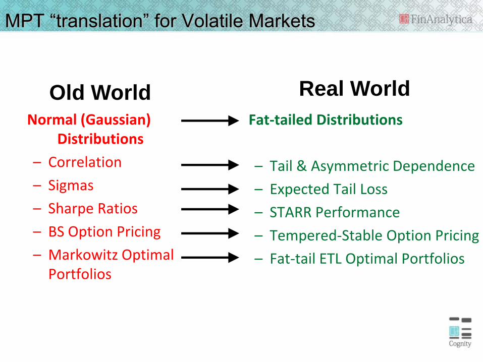
MPT “translation” for Volatile Markets
Normal (Gaussian) Distributions
– Correlation
– Sigmas
– Sharpe Ratios
– BS Option Pricing
– Markowitz Optimal Portfolios
Fat‐tailed Distributions
– Tail & Asymmetric Dependence
– Expected Tail Loss
– STARR Performance
– Tempered‐Stable Option Pricing
– Fat‐tail ETL Optimal Portfolios
Old World Real World
Models Map
Agenda
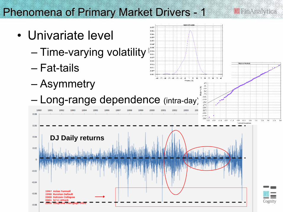
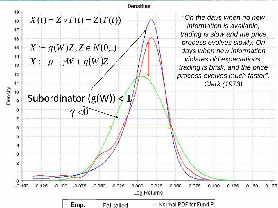
• The Fat-tailed Framework– Univariate model (single asset)
• Subordinated models• Stable model
– Dependence– Risk and Performance measures
• Applications– Option pricing - Some extension of the main fat-tailed
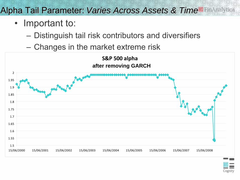
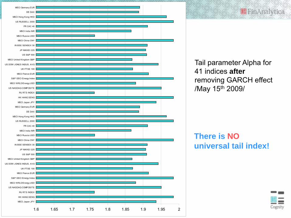
Tail parameter Alpha for 41 indices afterremoving GARCH effect/May 15th 2009/
1.6 1.65 1.7 1.75 1.8 1.85 1.9 1.95 2
MSCI Japan JPY
HK HANG SENG
RU RTS INDEX
US NASDAQ COMPOSITE
MSCI WRLD/Energy USD
S&P GSCI Energy Index
MSCI France EUR
UK FTSE 100
US DOW JONES INDUS. AVG
MSCI United Kingdom GBP
US S&P 500
JP NIKKEI 225
IN BSE SENSEX 30
MSCI China CNY
MSCI Russia USD
MSCI India INR
FR CAC 40
US RUSSELL 2000
MSCI Hong Kong HKD
DE DAX
MSCI Germany EUR
There is NOuniversal tail index!
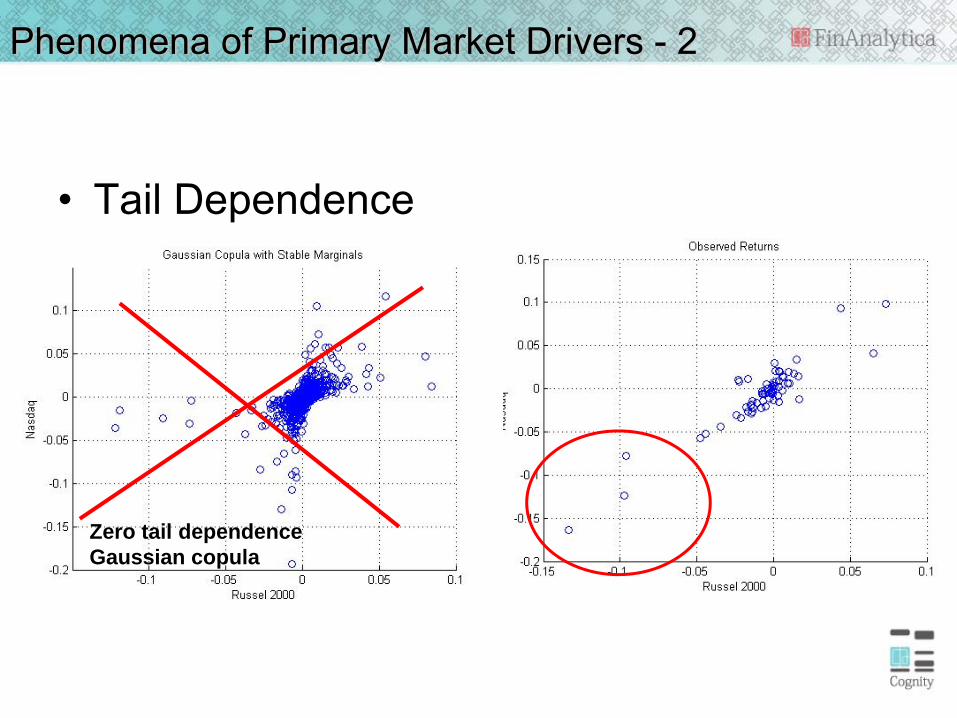
Phenomena of Primary Market Drivers - 2
• Tail Dependence
Zero tail dependenceGaussian copula
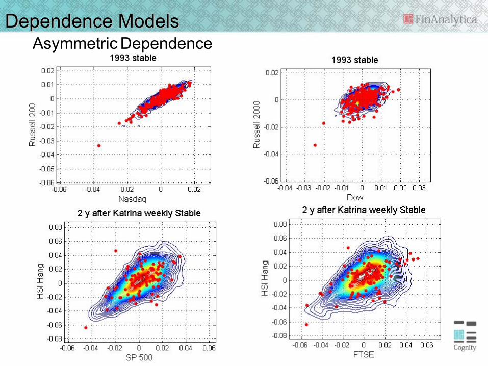
Dependence ModelsAsymmetric Dependence
Dependence ModelsModeling of Extreme Dependency in market crashes is critical for taking
correct investment decisionsBi-variate Normal
Fat-tailed indicesGaussian Copula
Fat-tailed indicesFat-tailed copula
Observed returns in Q3 1987
))(),...,((),...,( 111 nnn xFxFCxxF =
F is the multivariate cdf, C is the copula function and Fi are the one-dimensional cdf.
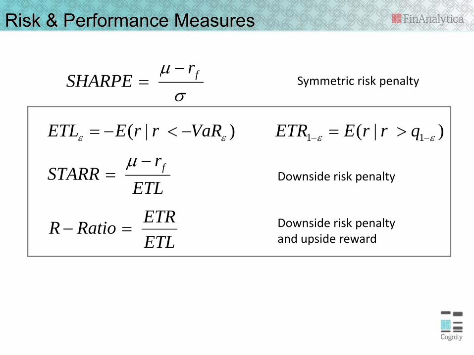
Risk & Performance Measures
Downside risk penaltyand upside reward
Symmetric risk penaltyσ
μ frSHARPE
−=
ETLr
STARR
qrrEETRVaRrrEETL
f−=
>=−<−= −−
μεεεε )|()|( 11
ETLETRRatioR =−
Downside risk penalty
Why not Normal ETL?
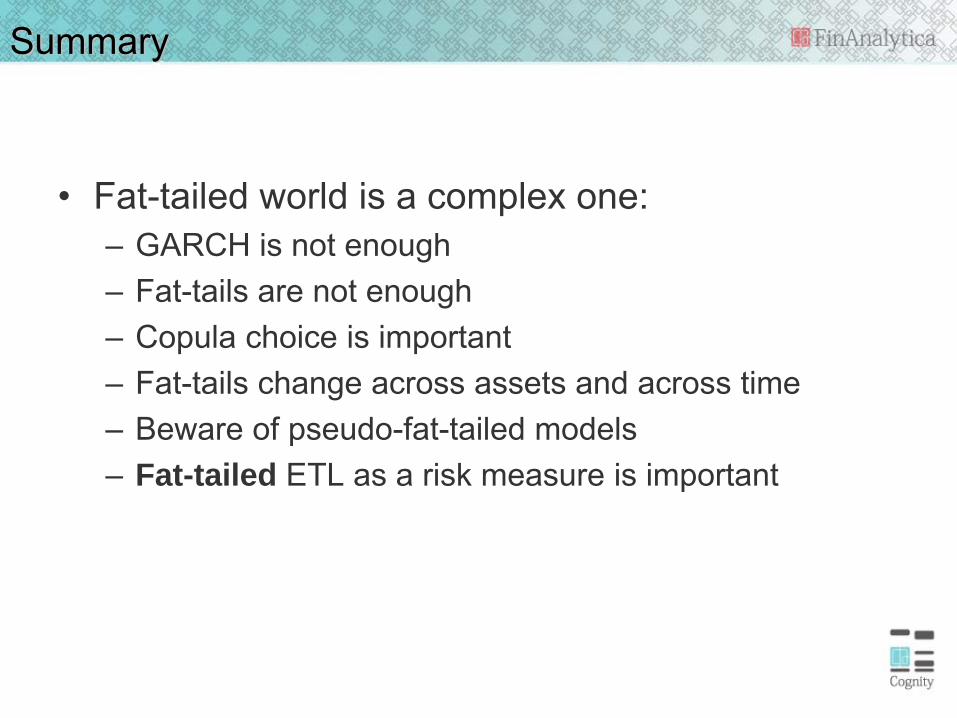
Summary
• Fat-tailed world is a complex one:– GARCH is not enough– Fat-tails are not enough– Copula choice is important– Fat-tails change across assets and across time– Beware of pseudo-fat-tailed models– Fat-tailed ETL as a risk measure is important
Application 1 – Option pricing Stable and Tempered Stable Distributions
Tempered Stable Models Introduction
• The stable model does not allow for unique equivalent martingale measure
• Take a stable model and make the very end of the tails lighter (still much heavier than the Gaussian)
• All moments exist• No-arbitrage option pricing exists
Tempered Stable
Tempered Stable
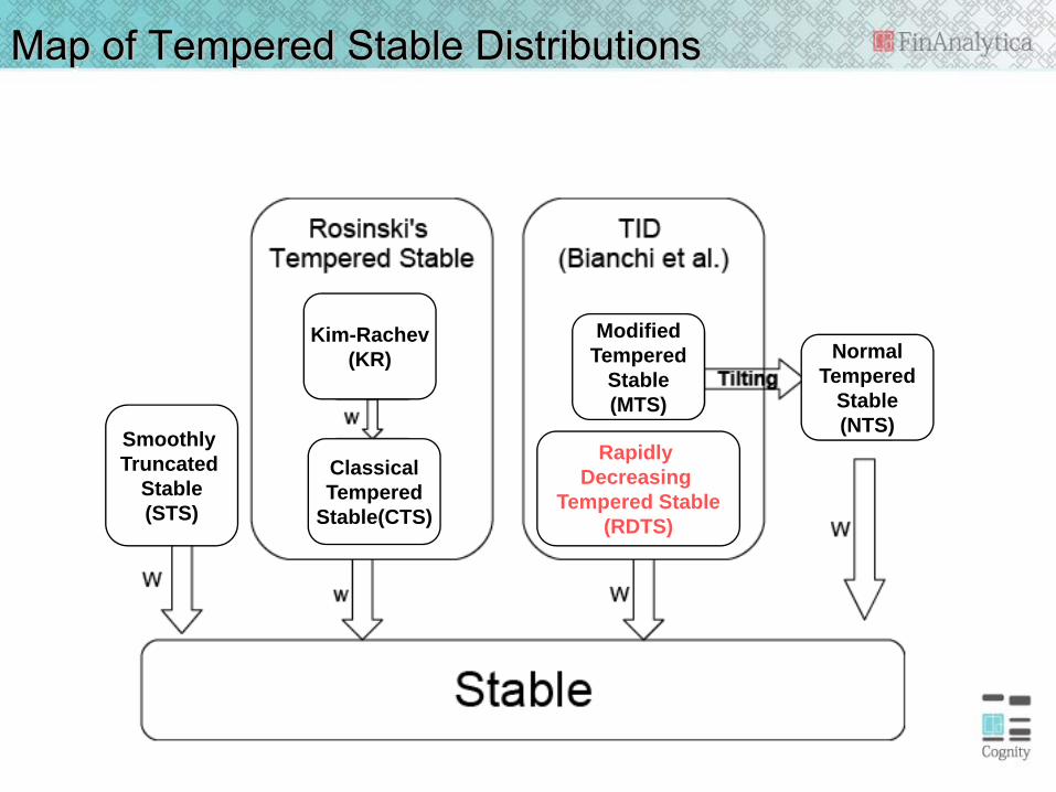
Map of Tempered Stable Distributions
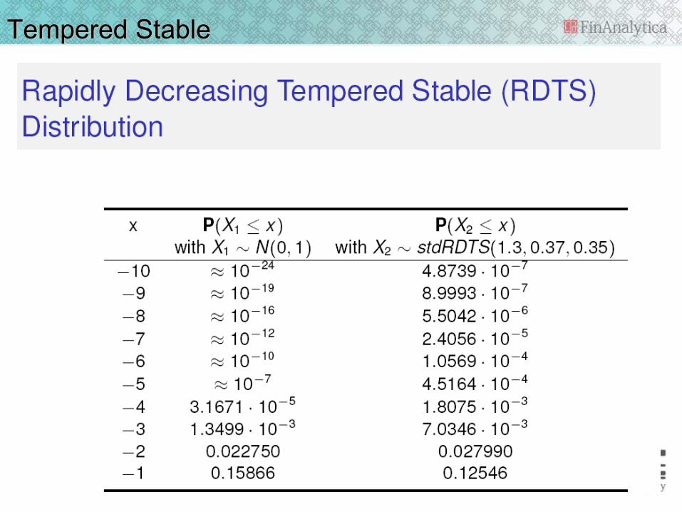
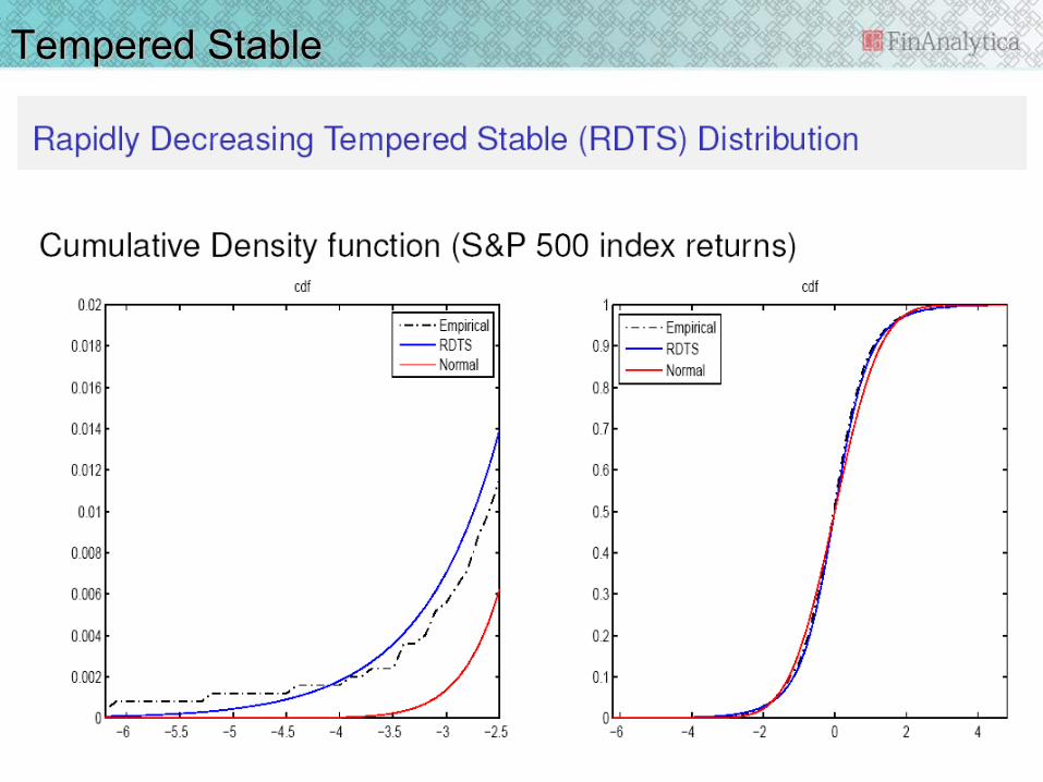
Rapidly Decreasing
Tempered Stable(RDTS)
Smoothly Truncated
Stable(STS)
Kim-Rachev(KR)
ClassicalTempered
Stable(CTS)
NormalTempered
Stable(NTS)
ModifiedTempered
Stable(MTS)
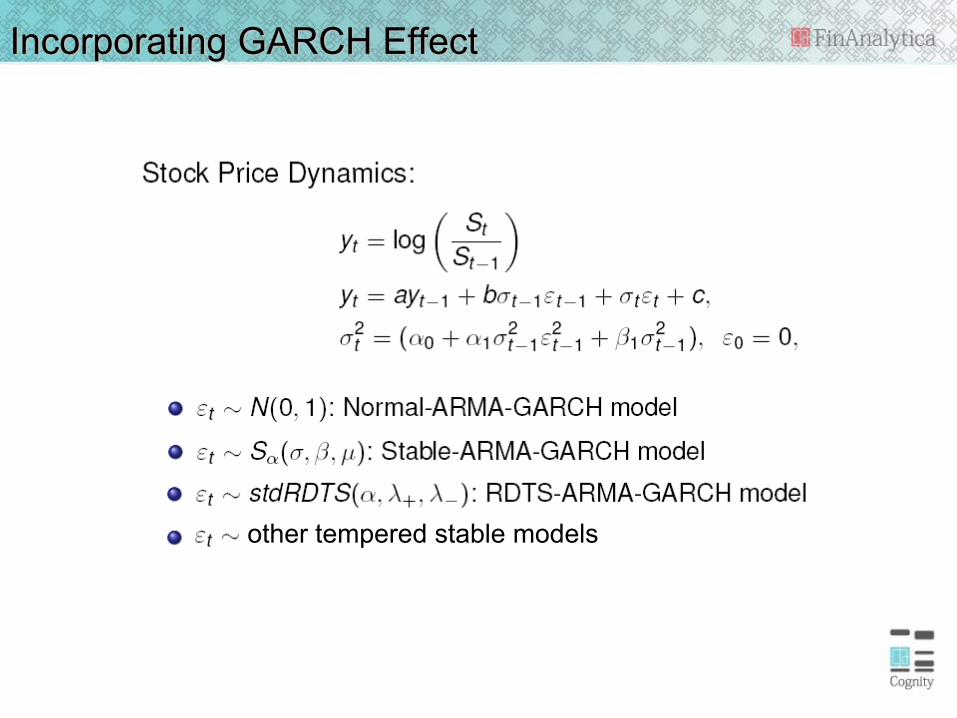
Incorporating GARCH Effect
other tempered stable models
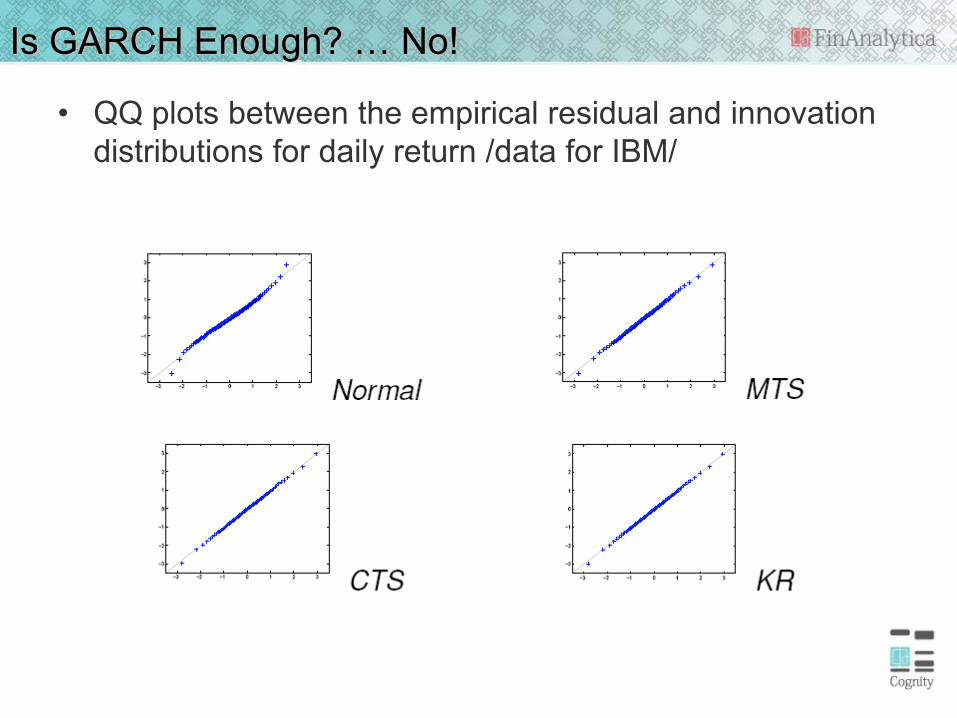
Is GARCH Enough? … No!
• QQ plots between the empirical residual and innovation distributions for daily return /data for IBM/
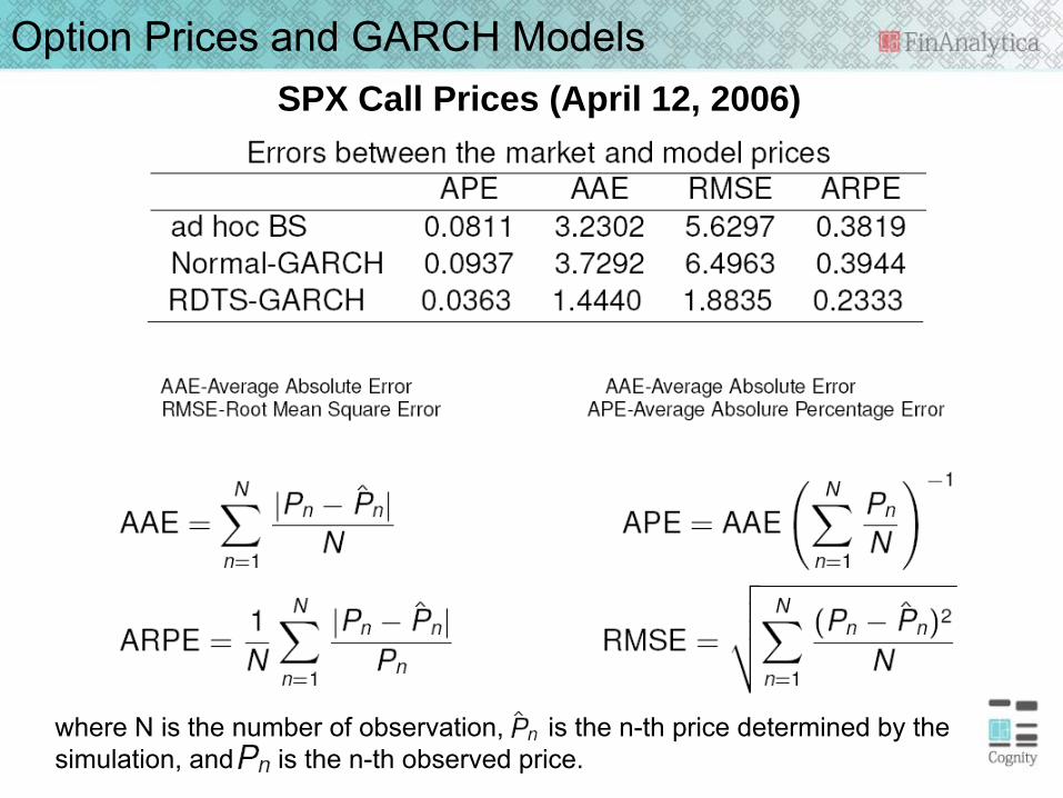
Option Prices and GARCH Models
where N is the number of observation, is the n-th price determined by thesimulation, and is the n-th observed price.
SPX Call Prices (April 12, 2006)
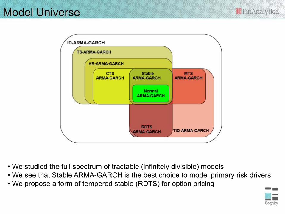
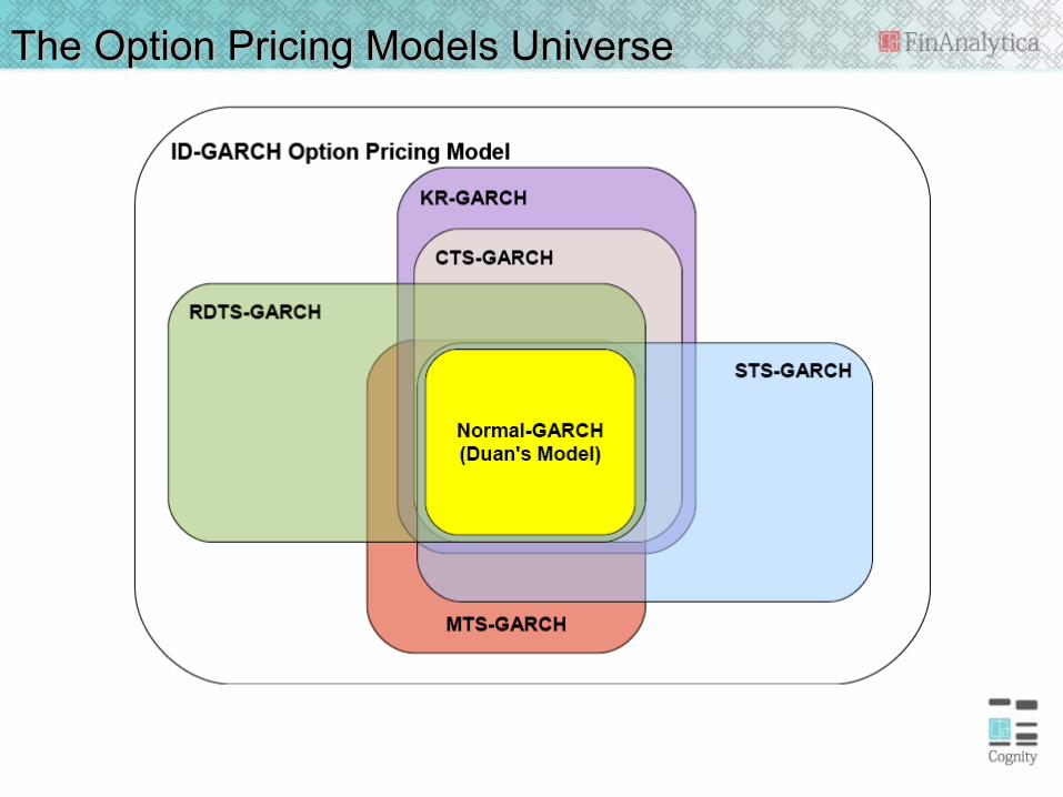
Model Universe
• We studied the full spectrum of tractable (infinitely divisible) models• We see that Stable ARMA-GARCH is the best choice to model primary risk drivers• We propose a form of tempered stable (RDTS) for option pricing
The Option Pricing Models Universe
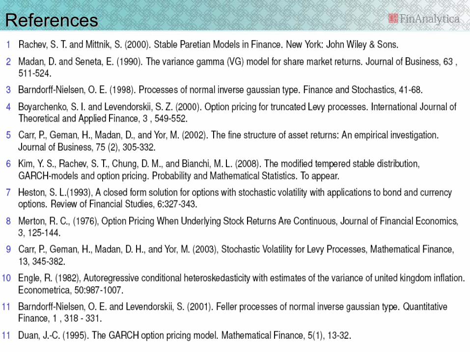
References
Application 2 - Modeling Market Crashes
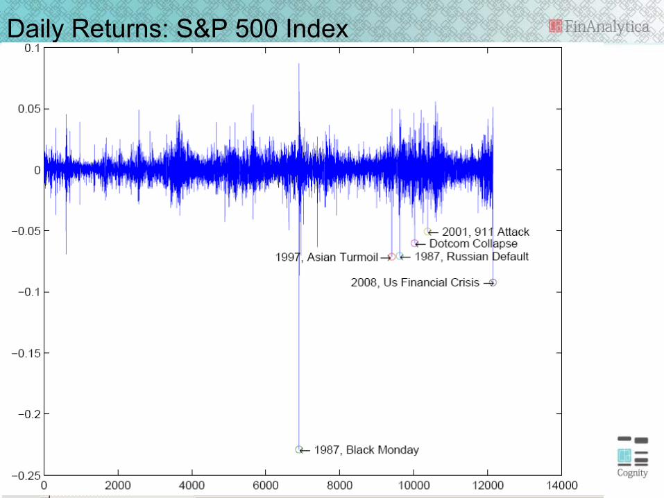
Daily Returns: S&P 500 Index
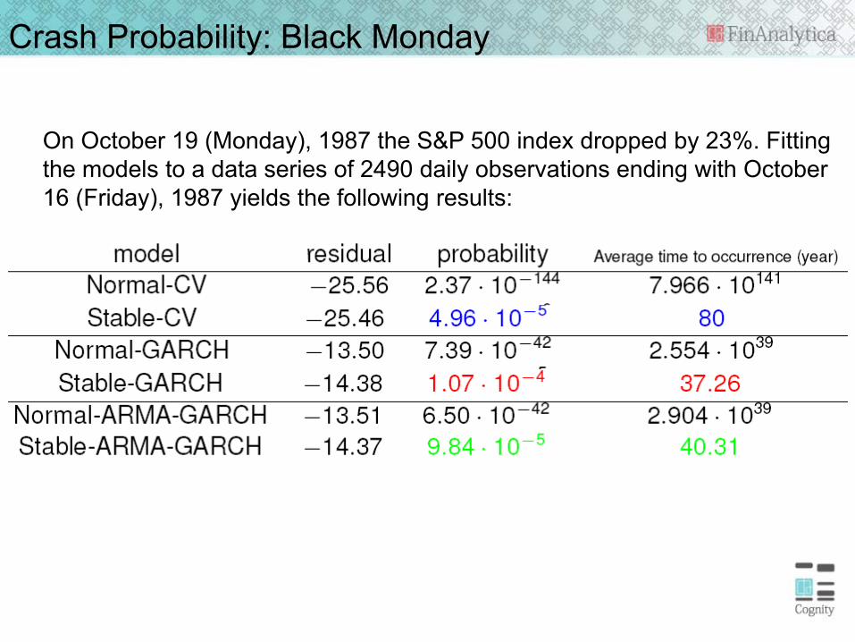
Crash Probability: Black Monday
On October 19 (Monday), 1987 the S&P 500 index dropped by 23%. Fitting the models to a data series of 2490 daily observations ending with October 16 (Friday), 1987 yields the following results:
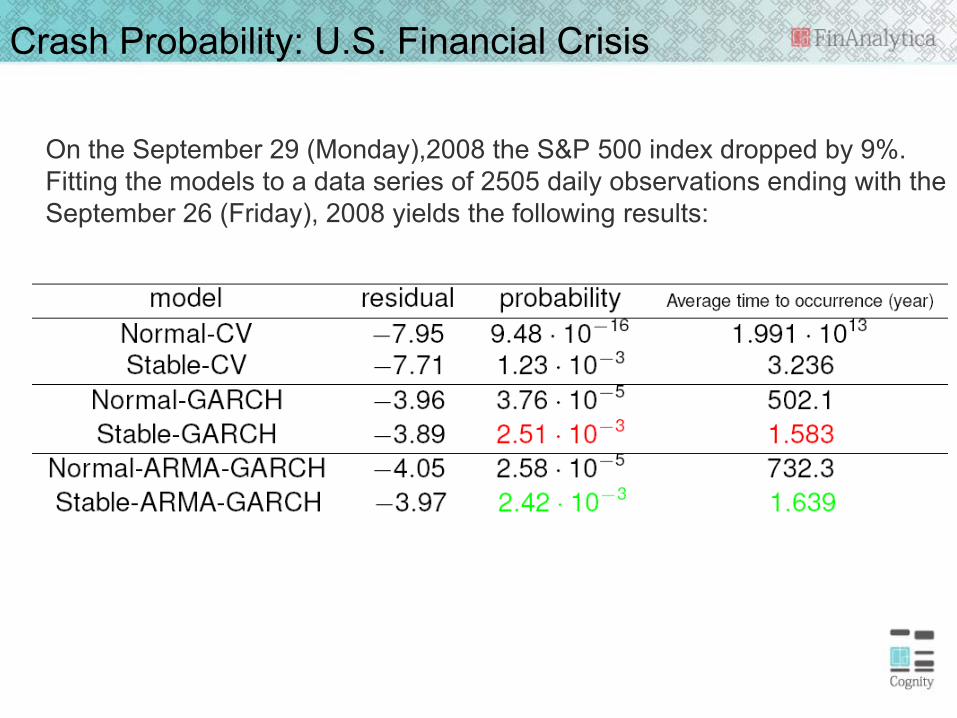
Crash Probability: U.S. Financial Crisis
On the September 29 (Monday),2008 the S&P 500 index dropped by 9%. Fitting the models to a data series of 2505 daily observations ending with the September 26 (Friday), 2008 yields the following results:
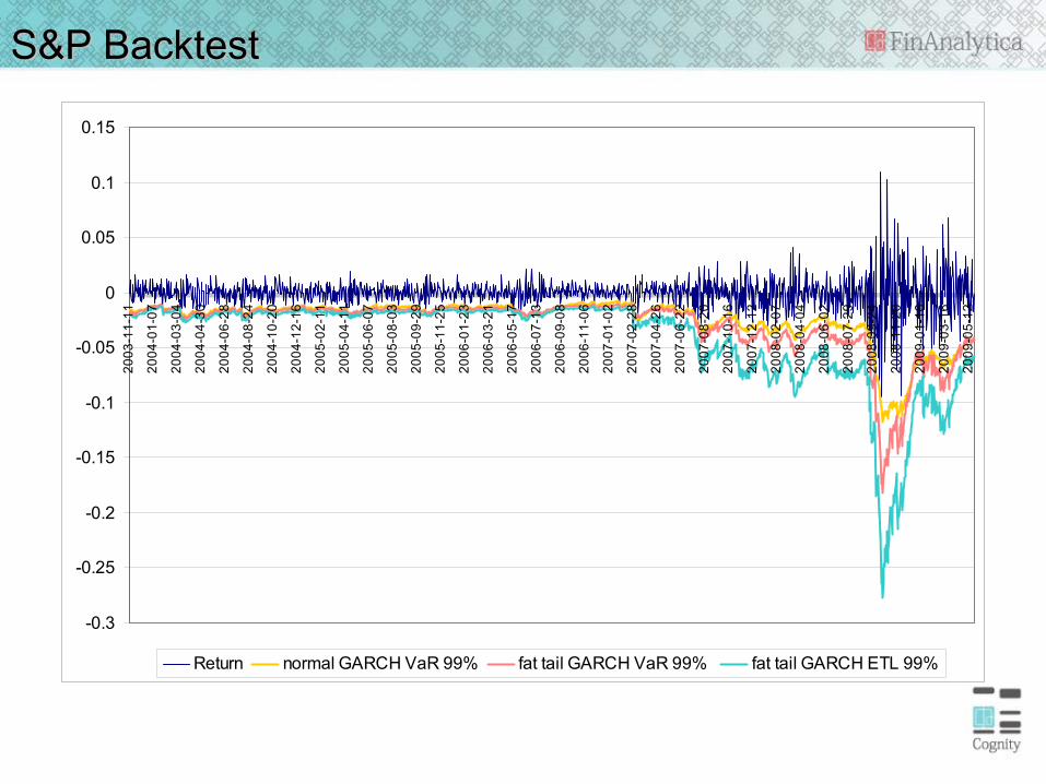
S&P Backtest
-0.3
-0.25
-0.2
-0.15
-0.1
-0.05
0
0.05
0.1
0.1520
03-1
1-11
2004
-01-
07
2004
-03-
04
2004
-04-
30
2004
-06-
28
2004
-08-
24
2004
-10-
20
2004
-12-
16
2005
-02-
11
2005
-04-
11
2005
-06-
07
2005
-08-
03
2005
-09-
29
2005
-11-
25
2006
-01-
23
2006
-03-
21
2006
-05-
17
2006
-07-
13
2006
-09-
08
2006
-11-
06
2007
-01-
02
2007
-02-
28
2007
-04-
26
2007
-06-
22
2007
-08-
20
2007
-10-
16
2007
-12-
12
2008
-02-
07
2008
-04-
04
2008
-06-
02
2008
-07-
29
2008
-09-
24
2008
-11-
20
2009
-01-
16
2009
-03-
16
2009
-05-
12
Return normal GARCH VaR 99% fat tail GARCH VaR 99% fat tail GARCH ETL 99%
References
Application 3 – Risk Monitoring
Backtest Example
• Long-short stock portfolio• 99% VaR backtest was run from 8/1/2007 to 5/15/2008
(206 days)• 250 rolling window used to fit the models• Models:
– Historical method– Normal method
• Constant Volatility• EWMA for Cov matrix
– Asymmetric Stable with Copula• Constant Volatility• Volatility Clustering
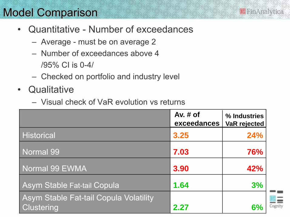
Model Comparison• Quantitative - Number of exceedances
– Average - must be on average 2– Number of exceedances above 4
/95% CI is 0-4/– Checked on portfolio and industry level
• Qualitative– Visual check of VaR evolution vs returns
Fat-tailed VaR with constant volatility provides long-term equilibrium VaR
Fat-tailed VaR with volatility clustering provides dynamic short-term view of the tail risk (VaR)
Both are important!
Returns
Normal 99
Normal 99 EWMA
Asym Stable Fat-tail Copula
Asym Stable Fat-tail Copula Vol Clustering
Risk Backtest
Application 4 – Portfolio Management and Optimization
Portfolio Risk Budgeting
• Marginal Contribution to RiskStandard Approach: St Dev
( ) cov( , )i i Pi
P P
r rMCTRσ σ
= =Ωw
Pi i P
i P
w MCTR σσ
σ∂ ′
⋅ = = =′∂∑ w Ωwww
( )( )ppii
i rVaRrrEw
ETLMCETL −≤−=∂
∂= |
The expression for marginal contribution to ETL is
and the resulting risk decomposition:
( )( ) ( )pi
ppiii
ii rETLrVaRrrEwMCETLw =−≤−=⋅ ∑∑ |
ETL:
Portfolio Optimization
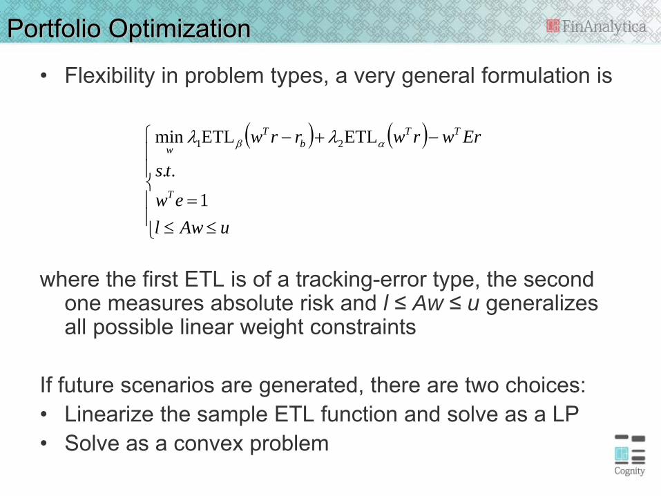
• Flexibility in problem types, a very general formulation is
where the first ETL is of a tracking-error type, the second one measures absolute risk and l ≤ Aw ≤ u generalizes all possible linear weight constraints
If future scenarios are generated, there are two choices: • Linearize the sample ETL function and solve as a LP• Solve as a convex problem
( ) ( )
⎪⎪
⎩
⎪⎪
⎨
⎧
≤≤=
−+−
uAwlew
ts
Erwrwrrw
T
TTb
T
w
1..
ETLETL min 21 αβ λλ
Portfolio Optimization References
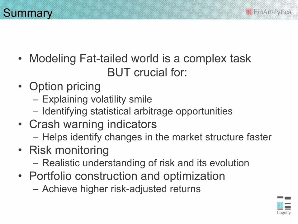
Summary
• Modeling Fat-tailed world is a complex taskBUT crucial for: