Key words. Emissions markets, Cap-and-trade schemes, Equilibrium models, Environmental Finance. MARKET DESIGN FOR EMISSION TRADING SCHEMES REN ´ E CARMONA * , MAX FEHR † , JURI HINZ ‡ , AND ARNAUD PORCHET § Abstract. The main thrust of the paper is the design and the numerical analysis of new cap- and-trade schemes for the control and the reduction of atmospheric pollution. The tools developed are intended to help policy makers and regulators understand the pros and the cons of the emissions markets. We propose a model for an economy where risk neutral firms produce goods to satisfy an inelastic demand and are endowed with permits by the regulator in order to offset their pollution at compliance time and avoid having to pay a penalty. Firms that can easily reduce emissions do so, while those for which it is harder buy permits from those firms anticipating that they will not need them, creating a financial market for pollution credits. Our model captures most of the features of the European Union Emissions Trading Scheme. We show existence of an equilibrium and uniqueness of emissions credit prices. We also characterize the equilibrium prices of goods and the optimal production and trading strategies of the firms. We choose the electricity market in Texas to illustrate numerically the qualitative properties observed during the implementation of the first phase of the European Union cap-and-trade CO 2 emissions scheme, comparing the results of cap- and-trade schemes to the Business As Usual benchmark. In particular, we confirm the presence of windfall profits criticized by the opponents of these markets. We also demonstrate the shortcomings of tax and subsidy alternatives. Finally we introduce a relative allocation scheme which despite of its ease of implementation, leads to smaller windfall profits than the standard scheme. 1. Introduction. Emission trading schemes, also known as cap and trade sys- tems, have been designed to reduce pollution by introducing appropriate market mech- anisms. The two most prominent examples of existing cap and trade systems are the EU-ETS (European Union Emission Trading Scheme) and the US Sulfur Dioxide Trading System. In such systems, a central authority sets a limit (cap) on the total amount of pollutant that can be emitted within a pre-determined period. To en- sure that this target is complied with, a certain number of credits are allocated to appropriate installations, and a penalty is applied as a charge per unit of pollutant emitted outside the limits of a given period. Firms may reduce their own pollution or purchase emission credits from a third party, in order to avoid accruing potential penalties. The transfer of allowances by trading is considered to be the core principle leading to the minimization of the costs caused by regulation: companies that can easily reduce emissions will do so, while those for which it is harder buy credits. In a cap-and-trade system, the initial allocation (i.e. the total number of al- lowances issued by the regulator) should be chosen in order for the scheme to reach a given emissions level. This total initial allocation is indeed the crucial parameter that the regulator uses as a knob to control the emission level. But while the value of the total initial allocation is driven by the emissions target, the specific distribution of these allowances among the various producers and market participants can be chosen * Department of Operations Research and Financial Engineering, Princeton University, Prince- ton, NJ 08544. Also with the Bendheim Center for Finance and the Applied and Computational Mathematics Program. ([email protected]). † Institute for Operations Research, ETH Zurich, CH-8092 Zurich, Switzerland ([email protected]). ‡ National University of Singapore, Department of Mathematics, 2 Science Drive, 117543 Singa- pore ([email protected]), Partially supported by WBS R-703-000-020-720 / C703000 of the Risk Management Institute at the National University of Singapore § Timbre J320, 15 Boulevard Gabriel Pri, 92245 MALAKOFF Cedex, FRANCE, ([email protected]). 1
RENE CARMONA ∗, MAX FEHR † , JURI HINZ ‡ , AND ARNAUD PORCHET §
Abstract. The main thrust of the paper is the design and the numerical analysis of new cap-and-trade schemes for the control and the reduction of atmospheric pollution. The tools developedare intended to help policy makers and regulators understand the pros and the cons of the emissionsmarkets. We propose a model for an economy where risk neutral firms produce goods to satisfy aninelastic demand and are endowed with permits by the regulator in order to offset their pollutionat compliance time and avoid having to pay a penalty. Firms that can easily reduce emissionsdo so, while those for which it is harder buy permits from those firms anticipating that they willnot need them, creating a financial market for pollution credits. Our model captures most of thefeatures of the European Union Emissions Trading Scheme. We show existence of an equilibrium anduniqueness of emissions credit prices. We also characterize the equilibrium prices of goods and theoptimal production and trading strategies of the firms. We choose the electricity market in Texasto illustrate numerically the qualitative properties observed during the implementation of the firstphase of the European Union cap-and-trade CO2 emissions scheme, comparing the results of cap-and-trade schemes to the Business As Usual benchmark. In particular, we confirm the presence ofwindfall profits criticized by the opponents of these markets. We also demonstrate the shortcomingsof tax and subsidy alternatives. Finally we introduce a relative allocation scheme which despite ofits ease of implementation, leads to smaller windfall profits than the standard scheme.
1. Introduction. Emission trading schemes, also known as cap and trade sys-tems, have been designed to reduce pollution by introducing appropriate market mech-anisms. The two most prominent examples of existing cap and trade systems are theEU-ETS (European Union Emission Trading Scheme) and the US Sulfur DioxideTrading System. In such systems, a central authority sets a limit (cap) on the totalamount of pollutant that can be emitted within a pre-determined period. To en-sure that this target is complied with, a certain number of credits are allocated toappropriate installations, and a penalty is applied as a charge per unit of pollutantemitted outside the limits of a given period. Firms may reduce their own pollutionor purchase emission credits from a third party, in order to avoid accruing potentialpenalties. The transfer of allowances by trading is considered to be the core principleleading to the minimization of the costs caused by regulation: companies that caneasily reduce emissions will do so, while those for which it is harder buy credits.
In a cap-and-trade system, the initial allocation (i.e. the total number of al-lowances issued by the regulator) should be chosen in order for the scheme to reach agiven emissions level. This total initial allocation is indeed the crucial parameter thatthe regulator uses as a knob to control the emission level. But while the value of thetotal initial allocation is driven by the emissions target, the specific distribution ofthese allowances among the various producers and market participants can be chosen
∗Department of Operations Research and Financial Engineering, Princeton University, Prince-ton, NJ 08544. Also with the Bendheim Center for Finance and the Applied and ComputationalMathematics Program. ([email protected]).
†Institute for Operations Research, ETH Zurich, CH-8092 Zurich, Switzerland([email protected]).
‡National University of Singapore, Department of Mathematics, 2 Science Drive, 117543 Singa-pore ([email protected]), Partially supported by WBS R-703-000-020-720 / C703000 of the RiskManagement Institute at the National University of Singapore
in order to create incentives to design and build cleaner and more efficient productionunits.
Naturally, emissions reduction increases the costs of goods whose productioncauses those emissions. Part or all of these costs are passed on to the end con-sumer and substantial windfall profits are likely to occur. Based on an empiricalanalysis of power generation profitability in the context of EU-ETS, strong empir-ical evidence of the existence of such profits is given in [14]. The authors of thisstudy come to the conclusion that power companies realize substantial profits sinceallowances are received for free while they are always priced into electrical power at arate that depends upon the emission rate of the marginal production unit: producersseem to take advantage of the trading scheme to make extra profit. This phenomenoncan even happen in a competitive setting. What follows is a simple illustration in adeterministic framework.
Let us consider a set of firms that must satisfy a demand of D = 1 MWh ofelectricity at each time t = 0, 1, · · · , T − 1, and let us assume that there are onlytwo possible technologies to produce electricity: gas technology which has unit cost2 $ and emits 1 ton of CO2 per MWh, and coal technology which has unit cost 1 $and emits 2 tons of CO2 per MWh. In this simple model, the total capacity of gasis 1 MWh and coal’s capacity is also 1 MWh. We also suppose that producers facea penalty π > 1 $ per ton of CO2 not offset by credits, and that a total of T − 1credits are distributed to the firms, allowing them to offset altogether T − 1 tons ofCO2. In this situation, we arrive at two conclusions. First, as demand needs to bemet, total emissions will be higher or equal than T tons, even if all firms use the cleantechnology (gas). Second, firms are always better off reducing emissions than payingthe penalty. As a consequence, the optimal generation strategy is to only use thegas technology and emit T tons of CO2. At least one firm has to pay the penalty,and the price of emission credits is necessarily equal to π at each time. Indeed themissing credit has a value π for both the buyer and the seller. The price of electricityis then 2 + π because a marginal decrease in demand will induce a marginal gain ingeneration cost and a marginal decrease of the penalty paid. The total profit for theproducers is π(T −1), the penalty paid by the producers to the regulator is π, and thetotal cost for the customers is (2 + π)T . Consider now the Business As Usual (BAU)situation: the demand is met by using coal technology, the price of electricity is 1, thetotal profit for producers is 0 and the total cost for the customers is T . In this simpleexample the producers cost induced by the trading scheme is T + π: producers mustbuy more expensive fuel, so a profit T is made by the fuel supplier and they have topay the penalty π. The increase in fuel price, or switching cost, is a marginal costthat must factor into the electricity price. The penalty is a fixed cost paid at the end,but we see that in this trading scheme, this fixed cost is rolled over the entire periodand paid by the customers at each time, inducing a windfall profit for the producers.This windfall profit is exactly equal to the market value of the T − 1 credits: thesecredits are given for free by the regulator but their market value is actually fundedby the customer.
Another feature of emissions trading schemes is the risk of non compliance facedby the producers and the regulator. The EU-ETS was introduced as a way of comply-ing with the targets set by the Kyoto Protocol. Phase 1 of the Kyoto Protocol sets afixed cap for annual emissions of CO2 by year 2012 to all industrialized countries thatratified the protocol (Annex I countries). This reduction should guarantee on averagea level of emissions of 95 % of what it was in year 1990. All countries are free to
Market Designs for Emissions Trading Schemes 3
adopt the emission reduction policy of their choice, but in case of non-compliance in2012, they face a penalty (payment of 1.3 emission allowances for each ton not offsetin Phase 1). The EU-ETS was designed to ensure compliance for the whole EU zone.However, in an uncertain environment, there exists the possibility that the schemewill fail its goal and that the producers will exceed the fixed cap set at the beginningof the compliance period. In this case, it is the regulator’s responsibility to com-ply with the target by buying allowances from other countries or generate additionalallowances by investing in clean projects under the Clean Development Mechanism(CDM for short) or the Joint Implementation (JI for short) mechanism, or otherwise,to pay the penalty. The design of emission trading schemes must also address thisquestion.
In the present work, we give a precise mathematical foundation to the analysis ofemission trading schemes and quantitatively investigate the impact of emission regu-lation on consumers costs and company’s profits. Based on an equilibrium model forperfect competition, we show that the action of an emission trading scheme combinestwo contrasting aspects. On the one hand, the system reduces pollution at the low-est cost for the society, as expected. On the other hand, it forces a notable transferof wealth from consumers to producers, which in general exceeds the social costs ofpollution reduction.
In a perfect economy where all customers are shareholders, windfall profits areredistributed, at least partially, by dividends. However, this situation is not thegeneral case and the impact of regulation on prices should be addressed. Thereare several other ways to return part of the windfall profits to the consumers. Themost prominent ones are taxation and charging for the initial allowance distribution.Beyond the political risks associated with new taxes, we will show that one of the maindisadvantages of this first method is its poor control of emissions under stochasticabatement costs. Concerning auctioning, it is important to notice that, in the firstphase of the EU-ETS, individual countries did not have to give away the totality oftheir credit allowances for free. They could choose to auction up to 10% of theirtotal allowances. Strangely enough, except for Denmark, none of them exercised thisoption. On the other hand using auctioning as a way to abolish windfall profits,one looses one of the main features of cap-and-trade schemes, namely the mechanismwhich allows to control the incentives to invest in and develop cleaner productiontechnologies. Indeed, a significant reduction of windfall profits through auctioning,if at all possible, requires that a huge amount or even the total initial allocationis auctioned. Further it involves a significant risk for companies since the capitalinvested to procure allowances at the auction may be higher than the income laterrecovered from allowances prices.
In this work, we argue that cap-and-trade schemes can work, even in the formimplemented in the first phase of EU-ETS, at least as long as allowance distribution isproperly calibrated. Moreover, we prove that it is possible to design modified emissiontrading schemes that overcome these problems. We show how to establish tradingschemes that reduce windfall profits while exhibiting the same emission reductionperformance as the generic cap and trade system used in the first implementationphase of the EU-ETS. These schemes also have the nice feature that a significantamount of the allowances can be allocated as initial allocation to encourage cleanertechnologies.
Despite frequent articles in the popular press and numerous speculative debatesin specialized magazines and talk-shows, the scientific literature on cap-and-trade
4 R. CARMONA, M. FEHR, J. HINZ AND A. PORCHET
systems is rather limited. We briefly mention a few related works chosen because oftheir relevance to our agenda. The authors of [3] and [9] proposed a market model forthe public good environment introduced by tradable emission credits. Using a staticmodel for a perfect market with pollution certificates, [9] shows that there exists aminimum cost equilibrium for companies facing a given environmental target. Theconceptual basis for dynamic permit trading is, among others, addressed in [2], [15],[11], [7], [12] and [13]. Meanwhile, the recent work [13] suggests also a continuous-timemodel for carbon price formation. Beyond these themes, there exists a vast literatureon several related topics, including equilibrium [1], empirical evidence from alreadyexisting markets [6], [14], and uncertainty and risk [5], [8], [16]. The model we presentbelow follows the baseline suggested in [4].
We close this introduction with a quick summary of the contents of the paper.Section 2 gives the details of the mathematical model used to capture the dynamic
features of a cap-and-trade system. We introduce the necessary notation to describethe production of goods and the profit mechanisms in a competitive economy. Ex-ogenous demand for goods is modeled by means of adapted stochastic processes. Weassume that demand is inelastic and has to be met exactly. This assumption couldbe viewed as unusually restrictive, but we argue that it is quite realistic in the caseof electricity. We also introduce the emissions allowance allocations and the rules oftrading in these allowances.
Section 3 defines the notion of competitive equilibrium for risk neutral firms in-volved in our cap-and-trade scheme. Preliminary work shows that most of the theoret-ical results of this paper still hold for risk averse firms if preferences are modeled withexponential utility. However, in order to avoid muddying the water with unnecessarytechnical issues which could distract the reader from the important issues of pollutionabatement, we restrict ourselves to the less technical case of risk neutral firms. Forthe sake of completeness, we solve the equilibrium problem in the Business As Usual(BAU from now on) case corresponding to the absence of market for emissions per-mits. In this case, as expected, the prices of goods are given by the standard meritorder pricing typical of deregulated markets. The section closes with the proof of acouple of enlightening necessary conditions for the existence of an equilibrium in ourmodel. These mathematical results show that at compliance time, the equilibriumprice of an emission certificate can only be equal to 0 or to the penalty level chosenby the regulator. The second important necessary condition shows that in equilib-rium, the prices of the goods are still given by a merit order pricing provided thatthe production costs are adjusted for the cost of emissions. This result is importantas it shows exactly how the price of pollution gets incorporated in the prices of goodsin the presence of a cap-and-trade scheme. The following Section 4 is devoted to therigorous proof of the existence of an equilibrium. The proof uses classical functionalanalysis results on optimization in infinite dimensional spaces. It follows the linesof a standard argument based on the analysis of what an informed central planner(representative agent) would do in order to minimize the social cost of meeting thedemand for goods.
Section 5 is devoted to the analysis of the standard cap-and-trade scheme featuredin the implementation of the first phase of the EU-ETS. By comparison with BAUscenarios, we show that properly chosen levels of penalty and pollution certificateallocations lead to desired emissions targets. However, our numerical experimentson a case study of the electricity market in Texas show the existence of excessivewindfall profits. As explained earlier in our literature review, these profits have been
Market Designs for Emissions Trading Schemes 5
observed in the first phase of EU-ETS, giving credibility to the critics of cap-and-trade systems. Section 6 can be viewed as the main thrust of the paper beyond thetheoretical results proven up to that point. We propose a general framework includ-ing taxes and subsidies along the standard cap-and-trade schemes. We demonstratethe shortcomings of the tax systems which suffer from poor control of the windfallprofits and unexpected expensive reduction policies when it comes to emissions re-duction targets under stochastic abatement costs. We concentrate our analysis onseveral new alternative cap-and-trade schemes and we show numerically that a rela-tive allocation scheme can resolve most of the issues with the other schemes. Such arelative allocation scheme is easy to describe and implement as pollution allowancesare distributed proportionally to production. Even though the number of permits israndom in a relative scheme, and hence cannot be known in advance, its statisticaldistribution is well understood as it is merely a scaled version of the distribution ofthe demands for goods. Consequently, setting up caps to meet pollution targets is notmuch different from the standard cap-and-trade schemes. Moreover, the coefficient ofproportionality providing the number of permits is an extra parameter which shouldmake the calibration more efficient. Indeed, one shows that properly calibrated, therelative schemes reach the same pollution targets as the standard schemes while atthe same time, they keep social costs and windfall profits in control.
Section 7 gathers more mathematical properties of the generalized cap-and-tradeschemes introduced in the previous section. Our results demonstrate the versatilityand the flexibility of such a generalized framework. It shows that regulators can con-trol cap-and-trade schemes in order to reach pre-assigned pollution targets with zerowindfall profits and reasonably small social costs, or even to force equilibrium elec-tricity prices to be equal to target prices. However, because of the level of complexityof their implementations, it is unlikely that the schemes identified there will be usedby policy makers or regulators. The paper concludes with Section 8 which reviewsthe main results of the paper recasting them in the perspective of the public policychallenging issues uncovered by the results of the paper.
2. Standard Cap-and-Trade Scheme. In this section we present the elementsof our mathematical analysis. We consider an economy where a set of firms produceand supply goods to end-consumers over a period [0, T ]. The production of these goodsis a source of pollutant emissions. In order to reduce this externality, a regulatordistributes emissions allowances to the firms at time 0, allows them to trade theallowances on an organized market between times 0 and T , and at the end of thiscompliance period, taxes the firms proportionally to their net cumulative emissions.
In what follows (Ω,F , Ft, t ∈ 0, 1, . . . , T, P) is a filtered probability space.We denote by E[.] the expectation operator under probability P and by Et[.] theexpectation operator conditional to Ft. The σ-field Ft represents the informationavailable at time t. We will also make use of the notation Pt(.) := Et[1.] for theconditional probability with respect to Ft.
2.1. Production of Goods. A finite set I of firms produce and sell a set Kof different goods at times 0, 1, . . . , T − 1. Each firm i ∈ I has access to a set J i,k
of different technologies to produce good k ∈ K, that are sources of emissions (e.g.greenhouse gases ). Each technology j ∈ J i,k is characterized by:
• a marginal cost Ci,j,kt of producing one unit of good k at time t;
• an emission factor ei,j,k measuring the volume of pollutants emitted per unitof good k produced by firm i with technology j;
• a production capacity κi,j,k.
6 R. CARMONA, M. FEHR, J. HINZ AND A. PORCHET
For the sake of notation we introduce the index sets
Mi = (j, k) : k ∈ K, j ∈ J i,k, i ∈ I ,
M = (i, j, k) : i ∈ I, k ∈ K, j ∈ J i,k .
In this paper, our main example of produced good is electricity. We make the assump-tion that the production costs are non-negative, adapted and integrable processes.
At each time 0 ≤ t ≤ T − 1, firm i ∈ I decides to produce throughout the period[t, t + 1) the amount ξi,j,k
t of good k ∈ K, using the technology j ∈ J i,k. Since thechoice of the production level ξi,j,k
t is based only on present and past observations, theprocesses ξi,j,k are supposed adapted and, since production cannot exceed capacity,we require that the inequalities
0 ≤ ξi,j,kt ≤ κi,j,k, i ∈ I, k ∈ K, j ∈ J i,k, t = 0, 1, · · · , T − 1, (2.1)
hold almost surely. Our market is driven by an exogenous and inelastic demand forgoods. Since electricity production is a significant proportion of the emissions coveredby the existing schemes, this inelasticity assumption is reasonable. We denote by Dk
t
the demand at time t for good k ∈ K. This demand process is supposed to be adaptedto the filtration Ftt. For each good k ∈ K, we assume that the demand is alwayssmaller than the total production capacity for this good, namely that:
0 ≤ Dkt ≤
∑i∈I
∑j∈Ji,k
κi,j,k almost surely, k ∈ K. (2.2)
This assumption is a natural extension of the assumption of inelasticity of the de-mand as it will conveniently discard issues such as blackouts which would only be adistraction given the purposes of the paper.
2.2. Emission Trading. We denote by π ∈ [0,∞) the penalty per unit of pol-lutant. For example, in the original design of the European Union Emissions TradingScheme (EU-ETS) π was set to 40€ per metric ton of Carbon Dioxyde equivalent(tCO2e). For each firm, the net cumulative emission is the amount of emissions whichhave not been offset by allowances at the end of the compliance period. It is com-puted at time T as the difference between the total amount of pollutants emitted overthe entire period [0, T ] minus the number of allowances held by the firm at time Tand redeemed for the purpose of emissions abatement. The net cumulative emissionis this difference whenever positive, and 0 otherwise.
For the sake of simplicity we assume that the entire period [0, T ] corresponds toone simple compliance period. In particular, at maturity T , all the firms have tocover their emissions by allowances or pay a penalty. Moreover, certificates becomeworthless if not used as we do not allow banking from one phase to the next. So in thiseconomy, operators of installations that emit pollutants will have two fundamentalchoices in order to avoid unwanted penalties: reduce emissions by producing withcleaner technologies or buy allowances.
At time 0, each firm i ∈ I is given an initial endowment of Λi0 allowances. So if
it were to hold on to this initial allowance endowment until the end, it would be ableto offset up to Λi
0 units of emissions, and start paying only if its actual cumulativeemissions exceed that cap level. This is the cap part of a cap-and-trade scheme.Depending upon their views on the demands for the various products and their riskappetites, firms may choose production schedules leading to cumulative emissions in
Market Designs for Emissions Trading Schemes 7
excess of their caps. In order to offset expected penalties, they may engage in buyingallowances from firms which expect to meet demand with less emissions than theirown cap. This is the trade part of a cap-and-trade schemes.
Remark 1. A first generalization of the above allowance distribution schemeis to reward the firms with allocations Λi
t at each time t = 0, 1, · · · , T − 1. Eventhough modeling EU-ETS would only require one initial (deterministic) allocation Λi
0
for each firm, we shall assume that the distribution of pollution permits is given byadapted stochastic processes Λi
tt=0,1,··· ,T−1. Indeed, all the theoretical results provenin the paper hold for these more general permit allocation processes since existence,uniqueness and characterization of the equilibrium price processes depend only uponthe total number of emission permits issued during the compliance period, not on theway the permits are distributed over time and among the various economic agents.
However as we will demonstrate, the statistical properties of social costs and wind-fall profits depend strongly on the way permits are allocated. The challenge faced bypolicy makers is to optimally design these allocation schemes to minimize social costswhile satisfying emissions reduction targets, controlling producers windfall profits andsetting incentives for the development of cleaner production technologies. We shallconcentrate on these issues in Sections 6 and 7.
Allowances are physical in nature, since they are certificates which can be re-deemed at time T to offset measured emissions. But, because of trading, thesecertificates change hands at each time t = 0, 1, · · · , T , and they become financialinstruments. However in general the allocation of allowances does not take place at asingle timepoint 0. For example, in EU ETS, allowances are allocated in March eachyear, while the 5 year compliance period starts in January. Therefore a significantamount of allowances are traded via forward contracts. Because compliance takesplace at time T , and only at that time, we will restrict ourselves to the situationwhere trading of emission allowances is done via forward contracts settled at time T .
Remark 2. Because compliance takes place at time T , a simple no-arbitrage ar-gument implies that the forward and spot allowance prices differ only by a discountingfactor, such that trading allowances or forwards gives the same expected discountedpayoff at time T . Therefore under the equilibrium definition that will be introducedin Section 3, considering only forward trading yields no loss of generality. Moreoverallowing trading in forward contracts in our model provides a more flexible setting: itis more general than considering only spot trading, since it allows for trading pollutionpermits even before these allowances are issued and allocated. This turns out to be animportant feature when dealing with general allocation schemes.
We denote by At the price at time t of a forward contract guaranteeing delivery ofone allowance certificate at maturity T . The terminology price at time t is misleadingas there is no exchange of funds at time t. At is better seen as a strike than a pricein the sense that it is the price (in time T currency) at which the buyer at time t ofthe forward contract agrees to purchase the allowance certificate at time T .
Each firm can take positions on the forward market, and we denote by θit the
number of forward contracts held by firm i at the beginning of the time interval[t, t+1). As usual, θi
t > 0 when the firm is long and θit < 0 when it is short. We define
a trading strategy of firm i as an adapted process θitt=0,··· ,T . If we denote by f i
t
the quantity of forward contracts bought or sold at time t and throughout the period[t, t + 1), f i being an adapted process, the position at time t verifies: θi
t+1 = θit + f i
t .The net cash position resulting from this trading strategy, leading to a net position
8 R. CARMONA, M. FEHR, J. HINZ AND A. PORCHET
of θiT contracts at time T , is:
RAT (θ) := −
T∑t=0
f itAt =
T−1∑t=0
θit(At+1 −At)− θi
T AT . (2.3)
We here make the assumption that allowances can be traded until time T , whereasproduction of goods is decided at time t for the whole period [t, t + 1), so that thelast production decision occurs at time T − 1. This assumption is reasonable sinceproduction of good is a less flexible process than trading.
2.3. Profits. As we argued earlier, it is natural to work with T -forward al-lowance contracts because compliance takes place at time T . By consistency, it isconvenient to express all cash flows, position values, firm wealth, and good values intime T -currency. As a side fringe benefit, this will avoid discounting in the computa-tions to come. So we use for numeraire the price Bt(T ) at time t of a Treasury (i.e.non defaultable) zero coupon bond maturing at T . We denote by Sk
t t=0,1,··· ,T theadapted spot price process of good k ∈ K, and according to the convention statedabove, we shall find it convenient to work at each time t with the T -forward price
Skt = Sk
t /Bt(T )
and we skip the dependence in T from the notation of the T -forward price as T is theonly maturity we are considering.
Hence, a cash flow Xt at time t is equivalently valued as a cash flow Xt/Bt(T ) atmaturity T . So if firm i follows the production policy ξi = (ξi,j,k
t )k∈K j∈Ji,kT−1t=0 its
instantaneous revenues at time t from goods production is given by∑(j,k)∈Mi
(Skt − Ci,j,k
t )ξi,j,kt
and its time T -forward value is given by:∑(j,k)∈Mi
(Skt − Ci,j,k
t )ξi,j,kt
provided we set Ci,j,kt = Ci,j,k
t /Bt(T ). The total net gains from producing and sellinggoods are thus:
T−1∑t=0
∑(j,k)∈Mi
(Skt − Ci,j,k
t )ξi,j,kt . (2.4)
In order to hedge their production decisions, firms trade on the emissions marketby adjusting their forward positions in allowances. In addition, at maturity T , eachfirm i redeems allowances to cover its emissions and/or pay a penalty. Let
Πi(ξi) :=T−1∑t=0
∑(j,k)∈Mi
ei,j,kξi,j,kt (2.5)
be the actual cumulative emissions of firm i when it uses production strategy ξi.We also suppose that there exists another source of emissions on which firm i has
Market Designs for Emissions Trading Schemes 9
no control, denoted ∆i, and supposed to be an FT -measurable random variable. Ifwe think of electricity as one of the produced goods for example, the presence of thisuncontrolled source of emissions can easily be explained. Usually electricity producersare required to hold a reserve margin in order to respond to short time demand changesand to protect against sudden outages or unexpectedly rapid ramps in demand. Whenscheduling their plants it is not yet known how much of this reserve margin willbe used. Therefore in most markets there is an uncertainty on the exact emissionlevel when a production decision is made. Alternatively, we can see ∆i as a sinkof emissions, accounting for example for the credits gained from Clean DevelopmentMechanisms or Joint Implementation mechanisms. In this case it can take negativevalues. In a first reading ∆i can be thought of as being 0 for the sake of simplicity. Weshall see later in the paper that its presence helps characterizing the equilibrium ofthe economy and that it is a useful tool for modeling several variations of the model.Introducing the net amount Γi of allowances that producer i ∈ I can use to offset thescheduled emissions by
Γi = ∆i −T−1∑t=0
Λit (2.6)
the total penalty paid by firm i at time T is:
π(Γi + Πi(ξi)− θiT )+ . (2.7)
Combining (2.4) and (2.7) together with (2.3), we obtain the expression for theterminal wealth (profits and losses at time T ) of firm i:
LA,S,i(θi, ξi) :=T−1∑t=0
∑(j,k)∈Mi
(Skt − Ci,j,k
t )ξi,j,kt
+T−1∑t=0
θit(At+1 −At)− θi
T AT
− π(Γi + Πi(ξi)− θiT )+ . (2.8)
To emphasize the mathematical technicalities of the model, we underline the factthat demands and production costs change with time in a stochastic manner. Thestatistical properties of these processes are given exogenously, and are known at time0 by all firms. Moreover, we always assume that these processes satisfy the constraints(2.1) and (2.2) almost surely. Agents adjust their production and trading strategiesin a non-anticipative manner to their observations of the fluctuations in demand andproduction costs. In turn, the production and trading strategies ξi and θi becomerespectively adapted stochastic processes on the stochastic base of the demand andproduction costs.
3. Market Equilibrium. In this section, we follow the common apprehensionthat a realistic market state is described by prices which correspond to a so-calledmarket equilibrium, a situation, where the demand for each product is covered, allfinancial positions are in the zero net supply, and each firm is satisfied by its ownstrategy. We define such an equilibrium and provide necessary conditions for itsexistence.
10 R. CARMONA, M. FEHR, J. HINZ AND A. PORCHET
3.1. Definition of Equilibrium. For any 1 ≤ p ≤ ∞ and for any normedvector space F , we introduce the following space of adapted processes:
Lpt (F ) :=
(Xs)t
s=0; F -valued, ‖Xs‖ ∈ Lp(Fs), s = 0, . . . , t
. (3.1)
We also introduce the spaces of admissible production strategies:
U i :=
(ξit)
T−1t=0 ∈ L∞T−1(RMi); 0 ≤ ξi,j,k
t ≤ κi,j,k, t = 0, . . . , T − 1
,
U :=
ξ ∈∏i∈I
U i;∑i∈I
∑j∈Ji,k
ξi,j,kt ≥ Dk
t , k ∈ K, t = 0, · · · , T − 1
and the spaces of admissible trading strategies:
Vi(A) :=(θi
t)T+1t=1 , adapted, ‖RA
T (θi)‖ ∈ L1(FT )
V(A) :=∏i∈I
Vi(A).
In order to avoid problems with existence of expected values in (2.8), we suppose thatallowance demand and production costs are integrable:
assumption 1.
Γi ∈ L1, Cit = (Ci,j,k
t )(j,k)∈MiT−1
t=0 ∈ L1T−1(RMi) i ∈ I, (3.2)
In what follows, we also use a technical assumption on the nature of the uncontrolledemissions. Even though this assumption is not needed for most of the equilibriumexistence results, it will help us characterize the prices in equilibrium by ruling outpathological situations. This technical assumption states that up until the end of thecompliance period, there is always uncertainty about the expected pollution level dueto unpredictable events as described in Section 2.3 in the sense that conditionallyon the information available at time T − 1, the sum of all the Γi’s has a continuousdistribution. More precisely, we shall assume that
assumption 2. the FT−1-conditional distribution of∑
i∈I ∆i possesses almostsurely no point mass, or equivalently, for all FT−1-measurable random variables Z
P
∑i∈I
∆i = Z
= 0 (3.3)
As we already pointed out, this technical assumption will help us refine the statementsof some of the results leading to the equilibriums.
Following the intuition that given price processes A = AtTt=0 and S = (Sk
t )k∈KT−1t=0
each firm aims at increasing its own wealth by maximizing
(θi, ξi) 7→ E[LA,S,i(θi, ξi)], (3.4)
over its admissible investment and production strategies, we are led to define equilib-rium in the following way:
Definition 1. The pair of price processes (A∗, S∗) ∈ L1T (R) × L1
T−1(R|K|) arean equilibrium of the market if for each i ∈ I there exists (θ∗i, ξ∗i) ∈ Vi(A∗)×U i such
Market Designs for Emissions Trading Schemes 11
that:(i) All financial positions are in zero net supply, i.e.∑
i∈I
θ∗it = 0, t = 0, . . . , T (3.5)
(ii) Supply meets demand for each good∑i∈I
∑j∈Ji,k
ξi,j,kt = Dk
t , k ∈ K, t = 0, . . . , T − 1 (3.6)
(iii) Each firm i ∈ I is satisfied by its own strategy in the sense that
E[LA∗,S∗,i(θ∗i, ξ∗i)] ≥ E[LA∗,S∗,i(θi, ξi)] for all (θi, ξi) ∈ Vi(A∗)× U i. (3.7)
3.2. Equilibrium in the Business As Usual Scenario . When the penaltyπ is equal to zero, an equilibrium should correspond to the Business As Usual sce-nario. As we explain below, it is characterized by the classical merit order productionstrategy. At time t and for each good k, all the production means of the economy areranked by increasing production costs Ci,j,k
t . Demand is met by producing from thecheapest production means and good k’s equilibrium spot price is the marginal costof production of the most expensive production means used to meet demand Dk
t .More precisely, if (A∗, S∗) is an equilibrium, the optimization problem of firm i is
sup(θi,ξi)∈Vi(A∗)×Ui
E
T−1∑t=0
∑(j,k)∈Mi
(Skt − Ci,j,k
t )ξi,j,kt +
T−1∑t=0
θit(At+1 −At)− θi
T AT
.
Trading and production strategies are thus decoupled from each other and we are leftwith a classical competitive equilibrium problem where each firm maximizes
supξi∈Ui
E
T−1∑t=0
∑(j,k)∈Mi
(Skt − Ci,j,k
t )ξi,j,kt
, (3.8)
and the equilibrium prices S∗ are set so that supply meets demand. The solutionof this equilibrium problem is given by the following linear program for each goodk ∈ K:
((ξ∗i,j,kt )j∈Ji,k)i∈I = argmax((ξi,j,kt )
j∈Ji,k )i∈I
∑i∈I
∑j∈Ji,k
−Ci,j,kt ξi,j,k
t (3.9)
s.t.∑i∈I
∑j∈Ji,k
ξi,j,kt = Dk
t
ξi,j,kt ≤ κi,j,k for i ∈ I, j ∈ J i,k
ξi,j,kt ≥ 0 for i ∈ I, j ∈ J i,k.
for all times t, and the associated equilibrium prices are
S∗kt = maxi∈I, j∈Ji,k
(Ci,j,kt )1ξ∗i,j,k
t >0, (3.10)
12 R. CARMONA, M. FEHR, J. HINZ AND A. PORCHET
This is exactly the merit order pricing mechanism of electricity that can be observedin most deregulated electricity markets without emission trading scheme. Conversely,it is easily seen that the above prices together with the above strategies define anequilibrium. In Section 4 we will see that even under an emission trading scheme thedispatching of production among producers is still a merit order-like dispatching withcosts adjusted to take into account the mark-to-market value of emissions.
3.3. Necessary Conditions for the Existence of an Equilibrium. Beforeturning to the full characterization of the equilibriums, we present some necessaryconditions that will provide interesting insight.
Proposition 3.1 (Necessary Conditions). Let (A∗, S∗) be an equilibrium and(θ∗, ξ∗) an associated optimal strategies, then following conditions hold:(i) Then the allowance price A∗ is a bounded martingale with values in [0, π] such that
A∗T = 0 ⊇ Γ + Π(ξ∗) < 0, A∗
T = π ⊇ Γ + Π(ξ∗) > 0 (3.11)
up to sets of probability zero.(ii) If moreover Assumption 2 holds, then it follows that A∗ is almost surely given by
A∗t = πE[1Γ+Π(ξ∗))≥0|Ft] (3.12)
for all t = 0, . . . , T .(iii) The spot prices S∗k and the optimal production strategy ξ∗i correspond to a meritorder-type equilibrium with adjusted costs Ci,j,k
t + ei,j,kA∗t .
Proof. First let us show that A∗ has to be a martingale. This is seen as follows:if not, there exists a time t and a set A ∈ Ft of non-zero probability such thatEt[A∗
t+11A] > 1AA∗t (resp. <). Then for each agent i ∈ I the trading strategy given
by θis = θ∗is for all s 6= t and θi
t = θ∗it + 1A (resp θit = θ∗it − 1A) outperforms the
strategy θ∗i, contradicting the third property of an equilibrium.To prove (3.11) notice that according to the definition of the equilibrium, θ∗iT (ω)coincides for almost all ω ∈ Ω with the maximizer of
z → −A∗T (ω)z − π(Γi(ω) + Πi(ξ∗i)(ω)− z)+. (3.13)
As a consequence, we obtain A∗T ∈ [0, π] almost surely, since if A∗
T (ω) 6∈ [0, π] thenthere exists no maximizer to (3.13). Further, observe that if A∗
T (ω) ∈ (0, π] then themaximizer is less than or equal to Γi(ω) + Πi(ξ∗i)(ω) and if A∗
T (ω) ∈ [0, π) then themaximizer is greater than or equal to Γi(ω) + Πi(ξ∗i)(ω). This holds for each i hencefollowing inclusions are satisfied almost surely
A∗T ∈ (0, π] ⊆ ∩i∈Iθ∗iT ≤ Γi + Πi(ξ∗) ⊆
∑i∈I
θ∗iT ≤ Γ + Π(ξ∗) (3.14)
A∗T ∈ [0, π) ⊆ ∩i∈Iθ∗iT ≥ Γi + Πi(ξ∗) ⊆
∑i∈I
θ∗iT ≥ Γ + Π(ξ∗). (3.15)
That is
A∗T ∈ (0, π] ∩ Γ + Π(ξ∗) < 0 ⊆
∑i∈I
θ∗iT < 0, (3.16)
A∗T ∈ [0, π) ∩ Γ + Π(ξ∗) > 0 ⊆
∑i∈I
θ∗iT > 0. (3.17)
Market Designs for Emissions Trading Schemes 13
Observe that due to the first equilibrium condition∑
i∈I θ∗iT = 0, the events on theright hand sides of (3.16) and (3.17) are sets of probability zero which shows that theinclusions (3.11) hold almost surely. Condition (ii) is a direct consequence of (i) andAssumption 2.
Finally, the optimization problem of agent i can be written as:
supθi∈Ui
E
T−1∑t=0
∑(j,k)∈Mi
(Skt − Ci,j,k
t − ei,j,kA∗T )ξi,j,k
t
= sup
θi∈Ui
E
T−1∑t=0
∑(j,k)∈Mi
(Skt − Ci,j,k
t − ei,j,kA∗t )ξ
i,j,kt
(3.18)
thanks to the martingale property of A∗. Comparing the above optimization problemwith (3.8), we observe that the equilibrium can be seen as a competitive productionequilibrium with adjusted costs Ci,j,k
t + ei,j,kA∗t .
This concludes the proof.
The above results provide a better understanding of what a potential equilibriumshould be. The allowance price must always be in [0, π], which is very intuitive sincebuying an extra allowance at time t will result in a gain of at most π at time T .As highlighted in the previous section, the equilibrium in the BAU scenario can berelated to a global cost minimization problem. We shall see in the next section thatthe equilibrium in the presence of a trading scheme enjoys the property of socialoptimality in the sense that any equilibrium corresponds to the solution of a certainglobal optimization problem, where the total pollution is reduced at minimal overallcosts. We call this optimization problem the representative firm problem. Beyond theeconomic interpretation of social-optimality, the importance of the global optimizationproblem is that its solution helps calculate the allowance prices in equilibrium. Wenow explore this connection in detail.
4. Equilibrium and Global Optimality. In this section, we show rigorouslythe existence of an equilibrium as defined in Definition 1. We do so by re-framingthe problem as an equivalent global optimization problem involving a hypotheticalinformed central planner (which we call a representative agent). We prove the equiv-alence of the two approaches, and as a by-product of the necessary condition provenin the previous section, we derive the uniqueness of the allowance price process.
4.1. The Representative Agent Problem . For each admissible productionstrategy ξ = ξii∈I ∈ U , the overall production costs are defined as
C(ξ) :=T−1∑t=0
∑(i,j,k)∈M
ξi,j,kt Ci,j,k
t .
and the overall cumulated emissions as
Π(ξ) :=T−1∑t=0
∑(i,j,k)∈M
ei,j,kξi,j,kt . (4.1)
14 R. CARMONA, M. FEHR, J. HINZ AND A. PORCHET
Using the notation
Γ :=∑i∈I
Γi
for the aggregate uncontrolled emissions and allowance endowments, the total costsfrom production and penalty payments can be defined as
G(ξ) := C(ξ) + π(Γ + Π(ξ))+, ξ ∈ U . (4.2)
We introduce the global optimization problem
infξ∈U
E[G(ξ)] (4.3)
which corresponds to the objective of an informed central planner trying to minimizeoverall expected costs. Recall that ξ is admissible if ξ ∈ U , i.e. if the demand is metand the production constraints are satisfied. The reason for the introduction of thisglobal optimization problem is contained in the second necessary condition for theexistence of equilibrium.
Proposition 4.1. If (A∗, S∗) is an equilibrium with associated strategies (θ∗, ξ∗),then ξ∗ is a solution of the global optimization problem (4.3) .
Proof. Obviously, it suffices to show that
E(G(ξ∗)) ≤ E(G(ξ)) for all ξ ∈ U . (4.4)
In order to do so we notice that:
∑i∈I
E[LA∗,S∗,i(θ∗i, ξ∗i)] = E[ T−1∑
t=0
∑i,j,k∈M
(S∗kt − Ci,j,kt )ξ∗i,j,kt
+T−1∑t=0
(∑i∈I
θ∗it
)(A∗
t+1 −A∗t )−
(∑i∈I
θ∗iT
)A∗
T
− π∑i∈I
(Γi + Πi(ξ∗i)− θ∗iT )+]
= E[ T−1∑
t=0
∑k∈K
S∗kt
(∑i∈I
∑j∈Ji,k
ξ∗i,j,kt
)− C(ξ∗)
− π∑i∈I
(Γi + Πi(ξ∗i)− θ∗iT )+]
where we used the fact that in equilibrium,∑
i∈I θ∗it = 0 holds for all t = 0, . . . , Tdue to condition (i) of Definition 1. Next we use the convexity inequality
∑i∈I
x+i ≥
(∑i∈I
xi
)+
Market Designs for Emissions Trading Schemes 15
and once more the fact that the financial positions are in zero net supply to concludethat
∑i∈I
E[LA∗,S∗,i(θ∗i, ξ∗i)] ≤T−1∑t=0
∑k∈K
E[S∗kt Dkt ]− E[C(ξ∗)]
− πE[(∑
i∈I
Γi +∑i∈I
Πi(ξ∗i))+]
=T−1∑t=0
∑k∈K
E[S∗kt Dkt ]− E[C(ξ∗)]− πE[(Γ + Π(ξ∗))+]
=T−1∑t=0
∑k∈K
E[S∗kt Dkt ]− E[G(ξ∗)].
Now, for each ξ ∈ U we define θ(ξ) as
θit(ξ) = 0 for all i = 1, . . . , N , t = 0, . . . , T − 1,
θiT (ξ) = Γi + Πi(ξi)− Γ + Π(ξ)
|I|.
Repeating the above argument for (θ(ξ), ξ) yields∑i∈I
E[LA∗,S∗,i(θi(ξ), ξi)] =∑t,k
E[S∗kt Dk
t ]− E[G(ξ)]. (4.5)
Applying the third property (each agent is satisfied with its own strategy) of the(A∗, S∗) equilibrium to the optimal investment and production strategies (θ∗i, ξ∗i)and (θi(ξ), ξi) yields
E[G(ξ∗)] ≤∑t,k
E[S∗kt Dkt ]−
∑i∈I
E[LA∗,S∗,i(θ∗i, ξ∗i)]
≤∑t,k
E[S∗kt Dkt ]−
∑i∈I
E[LA∗,S∗,i(θi(ξ), ξ)] = E[G(ξ)].
This holds for all ξ ∈ U completing the proof.The existence of an optimal ξ for the global optimization problem (4.3) follows
from standard functional analytic arguments.Proposition 4.2. Under Assumption 1, there exists a solution ξ ∈ U of the
global optimal control problem (4.3).Our proof relies on two simple properties which we state and prove as lemmas for thesake of clarity. First, we note that L1 :=
∏i∈I L1
T−1(RM ), equipped with the norm
‖X‖ =T−1∑t=0
∑(i,j,k)∈M
E[|Xi,j,kt |]
is a Banach space with dual L∞ :=∏
i∈I L∞T−1(RM ), the duality form being given by
〈X, ξ〉 :=T−1∑t=0
∑(i,j,k)∈M
E[Xi,j,kt ξi,j,k
t ], X ∈ L1, ξ ∈ L∞.
16 R. CARMONA, M. FEHR, J. HINZ AND A. PORCHET
Next, we consider the weak∗ topology σ(L∞,L1) on L∞ (see [10]), namely the weakesttopology for which all the linear forms
L∞ 3 ξ 7−→ 〈X, ξ〉 ∈ R, (4.6)
for X ∈ L1 are continuous.Lemma 4.3. The real valued function
is lower semi-continuous for the weak∗ topology.Proof. Obviously, the real valued function
L∞ 3 ξ 7−→ E[C(ξ)]
is continuous for the weak∗ topology since it is of the form ξ 7−→ 〈X, ξ〉 for someX ∈ L1 since X = C = Ci,j,k
t is a fixed element in L1 by assumption. So we onlyneed to prove that the real valued function
L∞ 3 ξ 7−→ E[(Γ + Π(ξ))+] (4.8)
is lower semi-continuous. Using the fact that for any integrable random variable Xone has
E[X+] = sup0≤Y≤1
E[XY ]
one sees that
E[(Γ + Π(ξ))+] = sup0≤Y≤1
(E[ΓY ] + E[Y Π(ξ)])
and hence that the function (4.8) is the supremum of a family of continuous functionsince for fixed Y , E[ΓY ] is a constant and ξ 7−→ E[Y Π(ξ)] is continuous for the weak∗
topology by the very definition of this topology. Since the supremum of any familyof continuous functions is lower semi-continuous, this concludes the proof that (4.7)is lower semi-continuous.
Lemma 4.4. For the convex subset U of L∞ it holds that:(i) U is norm-closed in L1
(ii) U is weakly∗ closed in L∞.Proof. (i)If (ξn)n∈N is a sequence in U converging in L1 to some random vari-
able ξ, then (ξi,j,kt,n )n∈N converges in mean for each (i, j, k) ∈ M and t = 0, . . . , T −
1, and extracting a subsequence if necessary, one concludes that (ξi,j,kt,n )n∈N and
(∑
i∈I
∑j∈Ji,k ξi,j,k
t,n )n∈N converge almost surely to ξi,j,kt and
∑i∈I
∑j∈Ji,k ξi,j,k
t re-spectively, showing that the constraints defining U are satisfied in the limit, implyingthat ξ ∈ U .
(ii) Since U is a convex and a norm-closed subset of L1 it follows from the Hahn-Banach Theorem that U is the intersection of halfspaces Hξ,c = X ∈ L1|〈X, ξ〉 ≤ cwith ξ ∈ L∞ and c ∈ R such that U ⊆ H. Since L∞ ⊆ L1 it holds for each of thesehalfspaces Hξ,c that ξ ∈ L1. Thus we conclude that Hξ,c∩L∞ = X ∈ L∞|〈X, ξ〉 ≤ cis closed in (L∞, σ(L∞,L1)). Since by definition it holds that U ⊆ L∞ it follows thatU is given by the intersection of the sets Hξ,c ∩ L∞. Since any intersection of closedsets is closed we conclude that U is weakly∗ closed in L∞.
Market Designs for Emissions Trading Schemes 17
Proof of Proposition 4.2 Since U is bounded and weakly∗ closed due to Lemma 4.4, itfollows from the Theorem of Banach-Alaoglu that U is weakly∗ compact. Lemma 4.3concludes the proof since any lower semi-continuous function attains its minimum ona compact set.
4.2. Relation with the Original Equilibrium Problem . As a consequenceof Assumption 2, for each production policy ξ ∈ U , no point masses occur in theFT−1-conditional distribution of Γ−Π(ξ). Hence, for all t = 0, . . . , T − 1 we have:
Pt(Γ + Π(ξ) ≥ 0) = Pt(Γ + Π(ξ) > 0). (4.9)
In the next theorem, we show that the value of the conditional probability in (4.9)characterizes the equilibrium allowance price at time t. To prepare for the proof ofthis result, we first prove a technical lemma.
Lemma 4.5. Let ξ be any solution of (4.6) whose existence is guaranteed byProposition 4.2, then it follows that:(i) For fixed t ∈ 0, . . . , T − 1 and any ξ ∈ U with ξs = ξs for all s = 0, . . . , t− 1
Et(G(ξ)) ≥ Et(G(ξ)) (4.10)
holds almost surely.(ii) If Assumption 2 is satisfied, then for each k ∈ K and i, i′ ∈ I, j ∈ J i,k, j′ ∈ J i′,k
it holds that
ξi,j,k
t ∈ [0, κi,j,k) ∩ ξi′,j′,k
t ∈ (0, κi′,j′,k]
⊆ Ci,j,kt + ei,j,kAt ≥ Ci′,j′,k
t + ei′,j′,kAt (4.11)
for all t = 0, . . . , T − 1 where At = πPt(Γ + Π(ξ) ≥ 0).Proof. (i) The assertion (4.10) is seen by the following argumentation: On the
contrary, one uses the Ft–measurable set
O := Et(G(ξ)) < Et(G(ξ) of positive measure P (O) > 0,
to outperform ξ by ξ′ as
ξ′s = 1Oξs + 1Ω\Oξs for all s = 0, . . . , T − 1. (4.12)
Note that since ξ and ξ′ coincide at times 0, . . . , t− 1, this definition indeed yields anadapted process ξ′ ∈ U . With (4.12), we have the decomposition
G(ξ′) = 1OG(ξ) + 1Ω\OG(ξ),
which gives a contradiction to the optimality of ξ:
E(G(ξ′)) = E(Et(1OG(ξ) + 1Ω\OG(ξ))
= E(1OEt(G(ξ)) + 1Ω\OEt(G(ξ)))
< E(1OEt(G(ξ)) + 1Ω\OEt(G(ξ))) = E(G(ξ)).
(ii) Introduce a deviation from the global optimal strategy ξ. At time t, consider ashift in production of ht units of the good k ∈ K, where the agents i ∈ I and i′ ∈ Iincrease/decrease their outputs from technologies j ∈ J i,k, j′ ∈ J i′,k respectively.
18 R. CARMONA, M. FEHR, J. HINZ AND A. PORCHET
This results in the new policy ξ + χ where χ ∈ Πi∈IU i the deviation vanishes at alltimes with the exception of t and
χi,j,kt = ht, χi′,j′,k
t = −ht,
Consider
D(ξ, λ) =Et(G(ξ + λχ))− Et(G(ξ))
λ, λ ∈ (0, 1].
Approaching 0 by λ in the countable set (0, 1]∩Q we obtain by dominated convergencelimits for ei,j,k ≤ ei′,j′,k′ and ei,j,k ≥ ei′,j′,k′ as
holds almost surely, which is equivalent to (4.11).We can now turn to the main result of this section.Theorem 4.6. Under the above assumptions, the following hold:
(i) If ξ ∈ U is a solution of the global optimization problem (4.3), then the processes(A,S) defined by
At = πPt(Γ + Π(ξ) ≥ 0), t = 0, . . . , T (4.14)
and
Sk
t = maxi∈I, j∈Ji,k
(Ci,j,kt + ei,j,kAt)1ξi,j,k
t >0, t = 0, . . . , T − 1 k ∈ K, (4.15)
is a market equilibrium (in the sense of Definition 1), for which the associated pro-duction strategy is ξ.(ii) The equilibrium allowance price process is almost surely unique.
Market Designs for Emissions Trading Schemes 19
(iii) For each good k ∈ K, the price Sk
is the smallest equilibrium price for good k inthe sense that for any other equilibrium price process S∗k, we have S
k ≤ S∗k almostsurely.
Proof. (i) We show that (A,S) so defined forms an equilibrium by an explicitconstruction of firm investment strategies θ
i ∈ Vi(A) such that (θi, ξ
i) satisfies (3.5),
(3.6) and (3.7). Define
θi
t = 0 for all i = 1, . . . , N , t = 1, . . . , T − 1,
θi
T = Γi + Πi(ξi)− Γ + Π(ξ)
|I|.
Since conditions (3.5) and (3.6) are obviously fulfilled, we focus on (3.7). We firstshow that E[LA,S,i(θ
i(ξi), ξi)] ≥ E[LA,S,i(θi, ξi)] for all (θi, ξi) ∈ Vi(A) × U i, where
θi(ξi) is constant equal to 0 until time T − 1 and
θi
T (ξi) := Γi + Πi(ξi)− Γ + Π(ξ)|I|
.
We have:
E[LA,S,i(θi, ξi)] = E
T−1∑t=0
∑(j,k)∈Mi
(Sk
t − Ci,j,kt )ξi,j,k
t − θiT AT
− π(Γi + Πi(ξi)− θiT )+
]since A defined by (4.14) is a bounded martingale. For all ξi ∈ U i, we show that wecan maximize the above quantity by computing the maximum pointwise in θi insidethe expectation. In view of (4.14), when ω ∈ Γ + Π(ξ) < 0 we have ω ∈ AT (ω) = 0and the maximum of
z 7→ −zAT (ω)− π(Γi(ω) + Πi(ξi)(ω)− z)+ (4.16)
is attained on each point z ∈ [Γi(ω) + Πi(ξi)(ω),∞) showing that θi(ξi)(ω) is a
maximizer. On the other hand, when ω ∈ Γ + Π(ξ) ≥ 0, we have AT (ω) = π, themaximum of (4.16) is attained on each point z ∈ (−∞,Γi(ω) + Πi(ξi)(ω)], and onceagain, θ
i(ξi) is a maximizer. Notice for later reference that in both cases, the value
of the maximum of (4.16) is E[−(Γi + Πi(ξi))AT ].To finish the proof, we prove that E[LA,S,i(θ
i, ξ
i)] ≥ E[LA,S,i(θ
i(ξi), ξi)] for all ξi ∈ U i.
According to the above computation, we have:
E[LA,S,i(θi(ξi), ξi)]
= E
T−1∑t=0
∑(j,k)∈Mi
(Sk
t − Ci,j,kt )ξi,j,k
t − (Γi + Πi(ξi))AT
= E
T−1∑t=0
∑(j,k)∈Mi
(Sk
t − Ci,j,kt − ei,j,kAT )ξi,j,k
t − ΓiAT
= E
T−1∑t=0
∑(j,k)∈Mi
(Sk
t − Ci,j,kt − ei,j,kAt)ξ
i,j,kt − ΓiAT
. (4.17)
20 R. CARMONA, M. FEHR, J. HINZ AND A. PORCHET
We now show that the following inclusions hold almost surely:
Sk
t − Ci,j,kt − ei,j,kAt > 0 ⊆ ξi,j,k
t = κi,j,k, (4.18)
Sk
t − Ci,j,kt − ei,j,kAt < 0 ⊆ ξi,j,k
t = 0. (4.19)
Inclusion (4.19) is a direct consequence of Definition (4.15) of the price process S.Using this same Definition (4.15) and Lemma 4.5 we see that:
Sk
t > Ci,j,kt + ei,j,kAt
⊆⋃
i′∈I,j′∈Ji′,k
Ci′,j′,kt + ei′,j′,kAt > Ci,j,k
t + ei,j,kAt ∩ ξi′,j′,k
> 0
⊆⋃
i′∈I,j′∈Ji′,k
(ξi,j,k
t = κi,j,k ∪ ξi′,j′,k
t = 0)∩ ξi′,j′,k
> 0
⊆ ξi,j,k
t = κi,j,k .
These inclusions allow us to show that E[LA,S,i(θi(ξi), ξi)] ≤ E[LA,S,i(θ
i, ξ
i)], thus
completing the proof of (i).(ii) Proposition 3.1 gives the form of an equilibrium price. Due to Part (i) of
Proposition 3.1 and Proposition 4.1 to prove almost sure uniqueness of the allowanceprice process, it is sufficient to prove that for any two solutions ξ, ξ of the globaloptimization problem (4.3) we have:
P((Γ + Π(ξ) > 0 ∩ Γ + Π(ξ) > 0
)⋃(Γ + Π(ξ) < 0 ∩ Γ + Π(ξ) < 0
))= 1
(4.20)We know that these production strategies are solution of the global problem (4.3),that we rewrite as a linear programming problem:
infξ∈U, Z∈L1(FT )
Z≥Γ+Π(ξ)−θ0, Z≥0
E[C(ξ) + πZ] . (4.21)
Each solution (ξ?, Z?) of (4.21) satisfies
Z? = (Γ + Π(ξ?))+ (4.22)
almost surely. Assume now that there are two optimal solutions (ξ, Z) and (ξ, Z) ofthe above linear programming problem. Due to the linearity of (4.21) it follows thatany convex linear combination
(λξ + (1− λ)ξ, λZ + (1− λ)Z) (4.23)
is also a solution to (4.21) for all λ ∈ [0, 1]. In view of (4.22), we conclude that foreach λ ∈ [0, 1]
λ(Γ + Π(ξ))+ + (1− λ)(Γ + Π(ξ))+
=(λ(Γ + Π(ξ)) + (1− λ)(Γ + Π(ξ))
)+
holds almost surely. Since the above assertion is obviously violated on
Γ + Π(ξ) < 0 < Γ + Π(ξ) ∪ Γ + Π(ξ) > 0 > Γ + Π(ξ)
Market Designs for Emissions Trading Schemes 21
this union must have a probability 0, which together with Assumption 2 yields (4.20).(iii) Assume on the contrary that there exists an equilibrium price process S∗ with
S∗kt (ω) < Skt (ω) for all ω ∈ B (4.24)
for some t ∈ 0, 1, . . . , T − 1, B ∈ Ft, P (B) > 0 and k ∈ K. Let ξ∗ be thecorresponding equilibrium strategies. Since equilibrium allowance price A is uniqueit follows from (4.19) that
S∗kt − Ci,j,kt − ei,j,kAt < 0 ⊆ ξ∗i,j,kt = 0
up to sets of probability zero. Consequently we obtain∑i∈I
∑j∈Ji,k
ξ∗i,j,kt =∑i∈I
∑j∈Ji,k
ξ∗i,j,kt 1S∗kt ≥Ci,j,k
t +ei,j,kAt (4.25)
≤∑i∈I
∑j∈Ji,k
κi,j,k1S∗kt ≥Ci,j,k
t +ei,j,kAt
almost surely. Moreover it follows from (4.19) and (4.18) that∑i∈I
∑j∈Ji,k
κi,j,k1St>Ci,j,kt +ei,j,kAt (4.26)
=∑i∈I
∑j∈Ji,k
ξi,j,kt −
∑i∈I
∑j∈Ji,k
ξi,j,kt 1Sk
t =Ci,j,kt +ei,j,kAt
<∑i∈I
∑j∈Ji,k
ξi,j,kt
holds almost surely. In the last equality we used∑i∈I
∑j∈Ji,k
ξi,j,kt 1Sk
t =Ci,j,kt +ei,j,kAt(ω) > 0 for all ω ∈ Ω
which follows from the definition of S. Further due to (4.24) it holds that∑i∈I
∑j∈Ji,k
κi,j,k1S∗kt ≥Ci,j,k
t +ei,j,kAt(ω) (4.27)
≤∑i∈I
∑j∈Ji,k
κi,j,k1Skt >Ci,j,k
t +ei,j,kAt(ω) for all ω ∈ B.
From (4.25), (4.26) and (4.27) we conclude that there exists a C ⊆ B with∑i∈I
∑j∈Ji,k
ξ∗i,j,kt (ω) <∑i∈I
∑j∈Ji,k
ξi,j,kt (ω) = Dt(ω)
for all ω ∈ C, which implies that S∗ is no equilibrium product price.Remark 3. On the basis of what is known for merit-order equilibria with discon-
tinuous cost functions, we do not expect uniqueness of the price process S∗k.Remark 4. In the introduction, we referred to social costs as the costs of regu-
lation, i.e. the pollution reduction costs. We now give a formal definition of what wemean by social costs. For each regulatory allocation ((Λi
t)T−1t=0 )i∈I , and for any choice
22 R. CARMONA, M. FEHR, J. HINZ AND A. PORCHET
of an equilibrium production schedule ξ∗ ∈ U , we define the social costs SC as therandom variable given by the difference between the production costs G(ξ∗) under thisproduction schedule and the production costs incurred in the same random scenarioshad we used the BAU equilibrium production schedule. In other words, the social costsare given by the random variable:
SC = C(ξ∗)− C(ξ∗BAU ). (4.28)
Notice also that as defined, the social costs do not depend upon the trading strategiesof the individual firms in the emissions market.
Remark 5. The results of this section were derived under the assumption thatthe emission coefficients ei,j,k were constant. However, by mere inspections of theproofs, the reader will easily convince herself that all the results remain true if theseemission coefficients are instead adapted stochastic processes in L1
T−1(R).
5. Prices and Windfall Profits in the Standard Scheme. The previoussections were dedicated to the introduction and the mathematical analysis of what wecalled the standard emission trading scheme. This cap-and-trade scheme was chosenbecause it is representative of the EU-ETS implementation.
In this section, we focus on an economy where one single good is produced. Wechoose the example of electricity because the power sector is worldwide one of themost important sources of green house gases. We study the impact of regulation onspot prices and producers’ profits. In order to provide insight on the effects of cap-and-trade legislations, we performed numerical simulations of equilibrium prices andoptimal production schedules by solving the global optimization problem (4.3) usingdata from the Texas electricity market. Specifics about the numerical implementationare given in the Appendix at the end of the paper. We shall report numerical findingsfrom this case study throughout the remainder of the paper.
5.1. A Model for Electricity and Carbon Trading in Texas . To performnumerical simulations, we chose to focus on the electricity sector in Texas. Texas hasan installed capacity of 81855 MW, mainly split into gas-fired (51489 MW), coal-fired(23321 MW), and nuclear (9019 MW) power plants. These figures are based on theinstalled capacity in 2007, including also additional nuclear and coal fired power plantsthat are planned to come online for the next 7 years. Including upcoming capacityslightly changes the production stack and leads to more interesting results than usingthe actual 2007 installed capacity. Nuclear technology has close to zero emissions, andit is always running in base-load. The source of emission reduction thus essentiallycomes from fuel switching between gas and coal.
So for all practical purposes, our model for Texas can be assume to involve onegood, electricity, produced from two different technologies, gas and coal. Stochasticcosts of production are equal to Ci,j,k
t = HjP jt , where j ∈ g, c, Hj is the heat rate
of technology j and P jt is the corresponding fuel price. Dt stands for the electricity
demand from which nuclear capacity has already been subtracted. We set the emissionrates to 0.42 ton/MWh for gas technology (CCGT-like) and 0.95 ton/MWh for coaltechnology respectively. These average emission rates have been chosen to give afaithful representation of Texas’ park of power plants.
The global optimization problem reads:
infξ∈U
E
T−1∑t=0
(Cgt ξg
t + Cct ξc
t ) + π
(T−1∑t=0
(egξgt + ecξc
t )− Γ0
)+
Market Designs for Emissions Trading Schemes 23
under the constraint: ξgt + ξc
t = Dt for every time t. In the particular case of twotechnologies, we can proceed to the change of variable (ξg
t , ξct ) 7−→ (Et, Ct), where
Et = ecξct + egξg
t and Ct = Cct ξc
t + Cgt ξg
t
are respectively the total emission and the cost of production for the period [t, t +1). Using the constraint that the demand has to be met, we obtain an equivalentformulation in terms of an emission abatement problem:
minE≤E≤E
E
T−1∑t=0
(Dt(ecFt + Cct )− FtEt) + π
(T−1∑t=0
Et − Γ0
)+ (5.1)
where:
Et = eg min(Dt, κg) + ec(Dt − κg)+
Et = ec min(Dt, κc) + eg(Dt − κc)+
are respectively the maximal and emissions possible at time t, and
Ft :=Cg
t − Cct
ec − eg(5.2)
is the fuel spread per ton of CO2 (or abatement cost). The fuel spread F representsthe marginal switching cost necessary to decrease emissions by 1 unit. We observethat the above formulation (5.1) only involves 2 exogenous stochastic processes: Dand F . Finally, we set the aggregated uncontrolled emissions
∑i∈I ∆i infinitesimally
small to stay in the realm of the assumptions of Theorem 4.6, and solve the global op-timization problem by stochastic dynamic programming on a 2-dimensional trinomialtree. Details are given in the appendix at the end of the paper.
5.2. Electricity Prices Under the Standard Scheme. In this subsection, wediscuss the impact of the regulation on electricity prices. We already emphasized thatuniqueness of equilibrium electricity prices was not granted. However, we identifiedthe minimal price among all the possible equilibrium prices in Equation (4.15). Inwhat follows, we focus on this price.
!!""!##
Figure 5.1. Histograms of the consumer costs, social costs, windfall profits and penalty pay-ments under a standard trading scheme scenario.
24 R. CARMONA, M. FEHR, J. HINZ AND A. PORCHET
Equation (4.15) shows two sources of change in the spot price compared to busi-ness as usual. First, the marginal technology may be different: this induces a varia-tion in marginal cost. This variation is likely to be positive but a negative variationis possible. Suppose for example that in a BAU scenario, coal is started first butthat demand is high enough so that gas is the marginal technology. Suppose that inthe presence of the trading scheme, allowance price is high enough to induce a fuelswitch, so that gas is started first. Assume also that demand is high so that coal isthe marginal technology. In this case, the variation in marginal cost can be negative.The second source of variation is the price of pollution ei,j,kA∗
t for the marginal tech-nology. The producers pass through the cost of expected penalties to end-consumers.This second contribution is always positive and is such that the spot price under thetrading scheme is always greater than the spot price in BAU.
A possible interpretation of formula (4.15) is that the allowance price enters theelectricity price as the price of an additional commodity that is used for power genera-tion besides fuels. Producing the last infinitesimal unit of electricity at time t inducesnot only costs due to extra fuel consumption, but also increases the emissions by ei,j,k
and hence also the expected penalty at time T by ei,j,kA∗t . Consequently these costs
have to be covered by the end-consumers, for the marginal production of product kto be profitable. Since this amount is passed on to the endconsumer in each timestepthe consumer cost
∑T−1t=0 (S∗t − SBAU
t )Dt are much bigger than the penalty that isactually paid. As we will see in the following the consumer costs exceed also by farthe social cost of the scheme.
Figure 5.1 quantifies both the penalty payments and the consumer cost and com-pares them to social costs and windfall profits (as defined in the next section) undera standard trading scheme for the Texas electricity sector. The penalty and initialallocation for this example are π = 100$ and θ0 = 1.826×10⁸ allowances respectively.This allocation corresponds to a reduction target of 10%, i.e. 1.827× 10⁸t Carbon, tobe reached with 95% probability.
The results depicted in Figure 5.1 illustrate the major critic articulated by someof the opponents of the cap-and-trade systems. We observe that end consumer costs,are approximately more than 10 times higher than social costs due to the tradingscheme. Hence the consumers’ burden exceeds by far the the overall reduction costs,which gives rise for significant extra profits for the producers.
5.3. Windfall Profits and Penalty Under the Standard Scheme. As ex-plained above, the pricing mechanism of the standard emissions trading scheme in-duces a significant wealth transfer from consumers to producers.
Another way of understanding the extra profits made by the producers is to con-sider the windfall profits defined as follows. In the general framework of a standardcap-and-trade system with multiple goods introduced earlier, if ξ∗ is an optimal pro-duction strategy associated with the equilibrium (A∗, S∗), we define the target priceSk
t of good k as:
Skt := max
i∈I,j∈Ji,kCi,j,k
t 1ξ∗i,j,kt >0. (5.3)
This price is the marginal cost under the optimal production schedule without takinginto account the cost of pollution. We then define the windfall profits of firm i as:
T−1∑t=0
∑(j,k)∈Mi
(S∗kt − Skt )ξ∗i,j,kt ,
Market Designs for Emissions Trading Schemes 25
and the overall windfall profits as
WP =T−1∑t=0
∑k∈K
(S∗kt − Skt )Dk
t . (5.4)
These windfall profits measure the profits for the production of goods in excess overwhat the profits would have been, had the same dispatching schedule been used, andthe target prices (e.g. the marginal fuel costs) be charged to the end consumerswithout the cost of pollution.
Remark 6. Another reasonable definition of the windfall profits of firm i wouldbe
T−1∑t=0
∑(j,k)∈Mi
(S∗kt − Skt )ξ∗i,j,kt − π
(Γi −Πi(ξ∗i)
)+(5.5)
meaning that the penalty payments due to the scheme are withdrawn from the extraprofits. Since producers decide upon their production strategy and therewith the risk topay the penalty, we take the point of view that they should pay the penalty and not theendconsumer. However as can be seen in Figure 5.1 the penalty payments vanish incomparison to the windfall profits as defined in (5.4). Hence in practical applications,both definitions should give similar results.
Figure 5.1 shows the distribution of windfall profits as computed in the exampleof the Texas electricity market chosen for illustration purposes. We observe that thewindfall profits are in average almost 10 times higher than actual abatement costs.Furthermore it also shows that the costs of expected future penalty passed to thecustomers are much higher (4637 times) than the penalty actually paid. This isconsistent with the deterministic example presented in the introduction.
5.4. Incentives for Cleaner Technologies. Using (4.17) we see that the ex-pected profits and losses of firm i ∈ I in an equilibrium (A∗, S∗) with associatedproduction schedules ξ∗ are given by
E[LA∗,S∗,i(θ∗i, ξ∗i)] = E
[(−∆i +
T−1∑t=0
Λit)A
∗T
]
+ E
T−1∑t=0
∑(j,k)∈Mi
(S∗kt − Ci,j,kt − ei,j,kA∗
t )ξ∗i,j,kt
.(5.6)
As will be shown in Proposition 7.1, both the equilibrium price processes (A∗, S∗) andthe production strategies ξ∗ are preserved under a change of the regulatory allocationfrom ((Λi
t)T−1t=0 )i∈I to ((Λi
0)T−1t=0 )i∈I as long as
∑i∈I
T−1∑t=0
Λit =
∑i∈I
T−1∑t=0
Λit
holds almost surely. However, such an adjustment of the allocation changes the ex-pected profits and losses of producer i ∈ I by the amount:
E[(Λi
0 − Λi0)A
∗T
]. (5.7)
26 R. CARMONA, M. FEHR, J. HINZ AND A. PORCHET
Obviously this gives a relative (relative to Λi0) expected money transfer of
E
[∑i∈I
(Λi0 − Λi
0)+A∗
T
](5.8)
from producers with Λi0 − Λi
0 < 0 to producers with Λi0 − Λi
0 > 0. If the initial allo-cation is given depending on the type of production plant it is possible to utilize thismechanism to increase or decrease the incomes of clean and dirty plants respectively,i.e. the initial allocation can be used to adjust the incentives to build cleaner plants.Depending on the specific market this will often be the main incentive to build cleanplants.
This mechanism is one of the main features of cap and trade schemes and will ingeneral fail if auctioning is used to abolish windfall profits. First notice that even a100% auction can not always reduce windfall profits to zero. This becomes obviousin a market with a lot of nuclear power plants where coal is marginal the whole time.In such a market the producers of nuclear power make huge windfall profits but sincetheir emissions are zero they do not need any allowances. Hence the auction can onlycover the windfall profits due to the coal fired plants. Therefore using auctioning tocut windfall profits a huge amount if not all allowances of the initial allocation shouldbe auctioned. However in such a case, the regulator looses the instrument to controlabove incentives. Therefore in the next section we propose alternative cap and tradeschemes that not only reduce windfall profits to zero in average, but also providea considerable amount of allowances that can be used to adjust incentives to buildcleaner plants.
6. Alternative Designs of Emission Trading Schemes. The main objec-tives of emission trading schemes are both to force the market to reach a certain reduc-tion target, and at the same time, to give incentives to develop and build cleaner pro-duction facilities. In view of the shortcomings of the standard cap-and-trade schemedemonstrated in the last section, we propose alternative designs which fulfil both ob-jectives at low social costs, low windfall profits and hence low costs transfered to theconsumer.
This is possible because the mathematical theory developed in the previous sec-tions allows us to study emissions reduction policies that are different from the stan-dard EU-ETS scheme.
In the first Subsection 6.1 below, we introduce a general (and fairly complex)cap-and-trade scheme including taxes and subsidies. We argue that the theoreticalresults derived earlier in the paper for standard schemes, still hold in this more gen-eral situation. The remaining of the section is devoted to the identification and thecalibration of two of the simplest particular cases of interest. A relative scheme isintroduced in Subsection 6.2 and a tax scheme is introduced in Subsection 6.3. Thefinal Subsection 6.4 provides comparative statics highlighting the differences betweenthese schemes on the case study of the Texas electricity market.
6.1. General Market Designs for Emission Trading Schemes. We de-scribe the new regulator policies by first generalizing the allocation procedure. Be-yond the static allocation Λi
t for firm i at time t, the regulator is now allowed todistribute credits dynamically and proportionally to production. To be more specific,at each time 0 ≤ t < T , firm i is provided with an allocation
Λit = Xi
t +∑
(j,k)∈M(i)
Y i,j,kt ξi,j,k
t , (6.1)
Market Designs for Emissions Trading Schemes 27
where Xi and Y i,j,k are adapted processes in L1T−1(R). For the sake of generality we
let Y i,j,kt depend upon j. However in this case the opportunity to relate the number
of allowances to real emissions is lost.In addition, the regulator can also tax or subsidize the various firms by means of
financial incentives or disincentives similar to the credit endowments described above.In this case, the firms’ profits are lowered at time t by an amount
TSi = V it +
∑(j,k)∈M(i)
Zi,j,kt ξi,j,k
t , (6.2)
where V i and Zi,j,k are as before, adapted processes in L1T−1(R). Remark that V i
and Zi,j,k stand for a tax when positive and a subsidy when negative. Examples ofpositive Zi,j,k include fuel and CO2 taxes. The combination of V i and Zi,j,k allowsfor the introduction of alternative regulation such as a system of reward/penalty withrespect to a given production (or equivalently emission) target ξi,j,k. By charging thequantity
T−1∑t=0
∑(j,k)∈Mi
Zi,j,kt (ξi,j,k
t − ξi,j,k
t)
corresponding to V it = −
∑(j,k)∈Mi
Zi,j,kt ξi,j,k
t, the regulator can provide incentives
for firm i to stay close to a given production or emission strategy.Under such a generalized cap-and-trade scheme, the terminal wealth (or profits
and losses) of firm i ∈ I reads:
LA,S,i(θi, ξi) := −T−1∑t=0
V it +
T−1∑t=0
∑(j,k)∈Mi
(Skt − Ci,j,k
t − Zi,j,kt )ξi,j,k
t
+T−1∑t=0
θit(At+1 −At)− θi
T AT
− π
∆i + Πi(ξi)−T−1∑t=0
Xit +
∑(j,k)∈M(i)
Y i,j,kt ξi,j,k
t
− θiT
+
. (6.3)
Despite the obviously greater generality of the present framework, the proofs of theresults of Theorem 4.6 are sufficient to cover the analysis of this broader class oftrading schemes:
Proposition 6.1. If we set
Γi := ∆i −T−1∑t=0
Xit , ei,j,k
t := ei,j,k − Y i,j,kt , and Ci,j,k
t := Ci,j,kt + Zi,j,k
t (6.4)
for a set of adjusted parameters, then the results of Theorem 4.6 hold true in the caseof the the generalized cap-and-trade scheme of this subsection provided we replace theparameters of Theorem 4.6 by the adjusted parameters so-defined.
Proof. The proof of this proposition follows a straightforward adaptation of thearguments used in the previous sections and Remark 5 about stochastic emissionfactors.
28 R. CARMONA, M. FEHR, J. HINZ AND A. PORCHET
The present formulation gives a general framework for the analysis of a broaderclass of cap-and-trade schemes. We mostly focus on two important particular cases:1) the case where Zi,j,k
t ≥ 0 varies with i and j which represents a fuel or emissiontax scheme, and 2) the case where Zi,j,k
t ≤ 0 only depends on k, which correspondsto a subsidy for the production of good k.
For an equilibrium (A∗, S∗) of the generalized scheme with associated strategies(θ∗, ξ∗) it is straightforward to extend the definition of windfall profits of firm i as:
GWP i =T−1∑t=0
∑(j,k)∈Mi
(S∗kt − Skt )ξ∗i,j,kt −
T−1∑t=0
(V i
t +∑
(j,k)∈Mi
Zi,j,kt ξ∗i,j,kt
),
the overall windfall profits being then defined as
GWP =T−1∑t=0
∑k∈K
(S∗kt − Skt )Dk
t −T−1∑t=0
(V i
t + Dkt
∑i∈I,j∈Ji,k
Zi,j,kt
). (6.5)
The above discussion suggests that windfall profits could be reduced with a relativeallocation rule constant over time. This motivates the following analysis.
6.2. Cap-and-Trade Schemes with Relative Allowance Allocation. Apositive relative allocation for some product Y i,j,k
t = yk < 0 for some k ∈ K all i ∈ Iand those j ∈ J i,k can be seen as a subsidy for good k that is given in the form ofallowances rather than in cash. When producing one unit of good k, the marginalpenalty increases only by (ei,j,k − yk)A∗
t rather than by ei,j,kA∗t as in a standard
scheme. Thus the net marginal overall production costs of the firms are lower whencompared to the standard scheme. This should result in a decrease of the price of goodk. In the present subsection, we study the simplest generalized cap-and-trade schemetaking advantage of this mechanism. It applies this mechanism only for productionmeans J i,k
marg ⊆ J i,k which can be marginal (e.g. in the case of the electricity markets,this excludes nuclear plants) and is obtained by setting:
Y i,j,kt = yk1j∈Ji,k
marg ∈ R for all t = 0, . . . , T − 1
Xi0 = xi ∈ R , Xi
t = 0 for all t = 1, . . . , T − 1
V it = 0, Zi,j,k
t = 0 for all t = 0, . . . , T − 1
for all (i, j, k) ∈ M .In what follows, not only do we discuss this relative cap-and-trade scheme, but
we also gain new insight into the standard cap-and-trade scheme by treating it as arelative cap-and-trade scheme with yk = 0 for all k ∈ K.
But for any comparison of different cap-and-trade schemes to be meaningful, weneed to calibrate their respective parameters to common characteristics. We proceedto the discussion of such a calibration.
6.2.1. Calibration of the Parameters. The relative scheme has three regula-tory parameters. Using the notation of this section, they are: 1) the penalty π, 2) therelative allocation coefficients (yk)k∈K , 3) the total initial allocations x =
∑i∈I xi
given to the firms i ∈ I. In this subsection we show, using again the example ofthe Texas electricity market, how one should choose these parameters in order toguarantee an emissions reduction target with given probability while keeping the ex-pected windfall profits near zero and controlling the social costs to keep them as low
Market Designs for Emissions Trading Schemes 29
0.00.1
0.20.3
0.40.5
0.6
ye
1.7⋅108 1.8⋅108 1.9⋅108 2.0⋅108 2.1⋅108
x+E(yeD)
-10
-5
0
5
10
15
20
25
$/MWh
0.00.1
0.20.3
0.40.5
0.6
ye
1.7⋅108 1.8⋅108 1.9⋅108 2.0⋅108 2.1⋅108
x+E(yeD)
-10
-5
0
5
10
15
20
25
$/MWh
0.00.1
0.20.3
0.40.5
0.6
ye
1.7⋅108 1.8⋅108 1.9⋅108 2.0⋅108 2.1⋅108
x+E(yeD)
1.7⋅108
1.8⋅108
1.8⋅108
1.8⋅108
1.9⋅108
2.0⋅108
2.0⋅108
t CO2
0.00.1
0.20.3
0.40.5
0.6
ye
1.7⋅108 1.8⋅108 1.9⋅108 2.0⋅108 2.1⋅108
x+E(yeD)
1.7⋅108
1.8⋅108
1.8⋅108
1.8⋅108
1.9⋅108
2.0⋅108
2.0⋅108
t CO2
Figure 6.1. Windfall profits (left) and 95% percentile of total emissions (right) as functions of
the relative allocation parameter and the expected allocation. Here D =∑T−1
t=0 Det denotes the total
electricity demand over one compliance period.
as possible. In the particular simulation used to illustrate the strategy, we choose anemissions reduction target of 1.827× 10⁸ to be reached with probability 95%.
To gain a first insight into the numerics, we fix the penalty π at 100$. The leftpane of Figure 6.1 gives the expected windfall profits while the right pane gives the95% percentile of the total emissions for different values of the relative allocation coef-ficient (ye) and the expected total allocation. It appears that the expected allocationcontrols the amount by which carbon emissions are reduced, while the relative alloca-tion coefficient ye controls the windfall profits. Designing a cap-and-trade scheme withzero windfall profits and pre-decided emissions target levels can be done by choosingthe parameters of our relative scheme at the intersection of the zero windfall profitlevel set with the 1.827× 10⁸ emission percentile level set. This procedure is depictedin Figure 6.2. We find ye = 0.54 and
∑i∈I xi = 5.4× 10⁷.
30 R. CARMONA, M. FEHR, J. HINZ AND A. PORCHET
Figure 6.2. The left pane shows the level sets of the two plots of Figure 6.1. The blue and thered lines indicate level sets of the windfall profits and the 95% quantile of emissions respectively.The right pane gives the plots of the overall production costs for electricity for one year as functionof the penalty level for both the absolute and relative schemes. The free regulatory parameters arechosen to guarantee the desired emissions percentile, and in the case of the relative scheme, suchthat the windfall profits are zero.
Since for the standard cap-and-trade scheme the parameter ye = 0 is fixed, wehave one less regulatory parameter. Thus controlling the emissions level by the initialallocation, we are not able to control the windfall profits. Hence the desired parametervalues are obtained at the intersection of the 1.827× 10⁸ emission percentile level setwith ye = 0. Giving the initial allocation
∑i∈I xi = 1.826× 10⁸.
Repeating the above procedure for different penalties levels gives regulatory set-tings with different production costs for the relative and the standard scheme in Figure6.2. Obviously for both schemes the social costs are reduced by increasing penalty.As shown in the right pane of Figure 6.2, this decrease in social costs is significantuntil the penalty reaches the level π = 100$. after that, the social costs stay nearlythe same, becoming independent of π for larger values of π. Hence, we conclude thatin this setting a penalty of 100$ is a reasonable choice for both the relative and thestandard scheme.
6.3. Emission Taxes. A static tax scheme is a regulation that penalizes theemission of each ton of carbon by a fixed amount, say z > 0. Formally, it can beviewed as a generalized scheme for which
Zi,j,kt = ei,j,kz , V i
t = 0Y k
t = 0 , Xit = 0
for all (i, j, k) ∈ M and t = 0, . . . , T − 1. Using the results of Proposition 6.1,we see that in such a tax scheme the prices of goods follow a merit order pricingrule with effective production costs given by Ci,j,k
t + ei,j,kz for all (i, j, k) ∈ M andt = 0, . . . , T − 1. The earnings under a tax scheme are based on the spread of theseeffective production costs. Since this spread does not depend solely on the originalfuel spread, it is in general not clear what windfall profits will be. It is not even clearif they are negative or positive. To gain some insight on this issue consider a tax of
Market Designs for Emissions Trading Schemes 31
z = 60$ (which is realistic for a 10% reduction target as will be seen below), andassume that at some point in time, the marginal production costs of coal and gas arethe same while all plants have to run to satisfy the demand. In this case the spreadin effective production cost is (ec − eg)z = 31.8$ and will be earned for each MWhthat is produced with gas. However, in the case of BAU, the earnings are zero. Hencethe windfall profits are 31.8$ per MWh of electricity produced with gas.
In tax schemes the only regulatory control parameter z should be adjusted in orderto guarantee a specified reduction target. Thus the windfall profits are automaticallygiven by the reduction target and can not be adjusted.
6.4. Comparison of the Various Abatement Schemes. We now comparethe characteristics of the standard and the relative cap-and-trade schemes with theregulatory parameters chosen in the previous subsection.
We first consider the windfall profits and the consumer costs. The results aregiven in Figure 6.3.
Figure 6.3. Histograms (computed from 500000 simulation scenarios) of the yearly distributionof windfall profits (left) and consumer costs (right) for the Standard Scheme, a Relative Scheme anda Tax Scheme.
As expected the relative scheme gives much lower consumer costs than the stan-dard scheme. This is related to the fact that the windfall profits have a narrowdistribution around zero in the case of the relative scheme, while the windfall profitsof the standard scheme are 10 times higher than the social costs. When comparedto the standard scheme, the only drawback of the relative scheme seems to be theslightly higher level of social costs which can be observed on the right pane of Figure6.4. However since this cost increase corresponds to approximately 0.4$ per MWhit is small in comparison to production costs and thus can be neglected in practice.Moreover those higher production costs are not just wasted money, they are paid forhigher emission reduction in many scenarios as can be seen on the left pane of Figure6.4. In particular the relative scheme takes advantage of cheap fuel switches when thestandard scheme cannot reduce emissions anymore. Moreover relative scheme is lesssensitive to weather, since in warm winters less allowances are allocated pushing theprice up. This in turn is responsible for higher emission abatements and consequently
32 R. CARMONA, M. FEHR, J. HINZ AND A. PORCHET
!
Figure 6.4. Yearly emissions from electricity production (left) for the Standard Scheme, theRelative Scheme, a Tax Scheme and BAU, and yearly abatement costs (right).
higher abatement costs.In this example approximately 30% of the allowances are given as initial allocation,
by allocating these to clean plants, further incentives can be set to build cleaner plants.This seems to be an important advantage of the relative scheme over other mechanismssuch as auctioning and tax.
Next, we study the effect of an emission tax on the Texas electricity market.Figure 6.4 shows that a pure tax scheme that fulfills the above reduction target of1.827×108tCO2 with 95% probability, is on average, more than twice (2.4×) as expen-sive as the standard cap and-trade-scheme. In other words, it has a poor emissionsreduction performance. These extra costs are paid for extra emission reductions.However in contrast with the results in the case of the relative scheme, the aver-age cost increase per reduced ton of carbon is considerable when we compare it tothe case of the standard scheme. The reason is that a tax is not flexible enough tocontrol emissions when abatement costs are stochastic. This results in an emissionuncertainty that exceeds even the BAU uncertainty with several orders of magnitude.Notice moreover that it carries a significant risk to reduce nearly no emissions. Insuch a scenario the tax corrections for upcoming years will be extremely expensive.Needless to say a tax scheme induces a huge money transfer from consumers to theregulator, which as can be seen in Figure 6.4 is even bigger than the costs transferredto the consumer in a standard cap and trade scheme.
7. More Financial Incentives. One of the main arguments in favor of therelative schemes studied in the previous section is the fact that they reduce windfallprofits. However, this reduction comes with slightly higher reduction costs than inthe case of the absolute scheme. While this cost increase is negligible in practice, it isof great theoretical interest to understand how and why one can design schemes thatgive exactly zero windfall profits at exactly the same reduction costs as the standardcap-and-trade scheme. In order to do so, we need to identify the generalized schemeswhich are in a one-to-one correspondence with the production policies of the standard
Market Designs for Emissions Trading Schemes 33
scheme. The latter are given by a subclass of generalized schemes for which Zi,j,kt
and Y i,j,kt depend only on k. The terminal wealth of firm i ∈ I under such a scheme
reads:
LA,S,i(θi, ξi) := −T−1∑t=0
V it +
T−1∑t=0
∑(j,k)∈Mi
(Skt − Ci,j,k
t − Zkt )ξi,j,k
t
+T−1∑t=0
θit(At+1 −At)− θi
T AT
− π
(∆i + Πi(ξi)−
T−1∑t=0
(Xi
t +∑
(j,k)∈M(i)
Y kt ξi,j,k
t
)− θi
T
)+
. (7.1)
The results of this section will demonstrate the versatility and the flexibility of thegeneralized framework introduced in this paper. However, because of the level ofcomplexity of their implementations, and despite the high degree of control theyprovide the regulator with, it is unlikely that the schemes identified here will be usedby policy makers or regulators.
7.1. Equilibria Equivalence. Our first result exhibits a one-to-one correspon-dence between the equilibria of standard schemes and generalized schemes leading toprofits and losses for firm i of the type (7.1).
Proposition 7.1. If (A∗, S∗) is an equilibrium with production strategies ξ∗ fora standard cap-and-trade scheme with adjusted uncontrolled emissions given by
Γi = ∆i −T−1∑s=0
(Xis + Ξi
s) for all i ∈ I, (7.2)
where Ξ is a stochastic process in L1T−1(R) such that
T−1∑t=0
∑i∈I
Ξit =
T−1∑t=0
∑k∈K
Y kt Dk
t , (7.3)
then the prices (A∗, S†) where
S†kt = S∗kt + Zkt − Y k
t A∗t for all k ∈ K, t = 0, . . . , T − 1 (7.4)
define an equilibrium of the generalized cap-and-trade scheme with the same productionstrategies ξ∗. The converse statement also holds.In particular if
T−1∑t=0
(∑i∈I
Xit +
∑k∈K
Y kt Dk
t
)=∑i∈I
Λi0
where Λi0 is the allocation in standard scheme, there is a one-to-one correspondence
between the generalized scheme and the standard scheme with initial allocation Λi0.
In particular, the lowest equilibrium product price is given by (7.4) where S∗ isgiven by Theorem 4.6 for the standard scheme with adjusted uncontrolled emissions(Γi)i∈I . To prove Proposition 7.1, we shall need the following lemma.
34 R. CARMONA, M. FEHR, J. HINZ AND A. PORCHET
Lemma 7.2. Let A be an integrable martingale, θ, θ′ ∈ Vi(A), ξi ∈ U i, and S, S′
be two integrable price processes, such that:
θ′it = θi
t for all t ≤ T − 1 (7.5)
θ′iT = θi
T −T−1∑t=0
(Ξi
t −∑
(j,k)∈M(i)
Y kt ξi,j,k
t
)(7.6)
S′kt = Sk
t + Zkt − Y k
t At for all k ∈ K, t = 0, . . . , T − 1
where Zk ≤ 0 is a subsidy, then we have:
E[LA,S,i(θi, ξi)] = E[HA,S′,i(θ′i, ξi)] + E
[T−1∑t=0
(V it − Ξi
tAt)
]. (7.7)
Proof. The martingale property of A yields:
E
θ′iT AT + π
∆i + Πi(ξi)−T−1∑t=0
(Xit +
∑(j,k)∈M(i)
Y kt ξi,j,k
t )− θ′iT
+= E
θiT AT +
T−1∑t=0
−Ξit +
∑(j,k)∈M(i)
ξi,j,kt Y k
t
E(AT |Ft)
+π
(∆i + Πi(ξi)−
T−1∑t=0
(Xit + Ξi
t)
)+
= E
θiT AT +
T−1∑t=0
∑(j,k)∈M(i)
ξi,j,kt Y k
t
At + π(Γi + Πi(ξi)− θi
T
)+− E(
T−1∑t=0
ΞitAt))
which proves the desired result.We can now turn to the proof of Proposition 7.1.Proof. Let (A∗, S∗) be equilibrium price processes of a standard scheme with
strategies (ξ∗, θ∗). Let θ′∗ be the adjusted optimal strategy as in Lemma 7.2. The
assertion follows by checking that conditions (i) to (iii) of Definition 1 are fulfilledby the pair of price processes (A∗, S†) and strategies (ξ∗, θ′∗). Since θ∗ satisfiesthe market clearing condition (3.5), so does θ′
∗. This proves (i) while condition (ii)follows directly from (7.3). Moreover, given (θ′, ξi) ∈ Vi(A∗)×U i, we define strategiesθi ∈ Vi(A∗) such that (7.5) and (7.6) hold. According to Proposition 3.1 A∗ is anintegrable martingale and the result of Lemma 7.2 yields
E[HA∗,S†,i(θ′i, ξi)] = E[LA∗,S∗,i(θi, ξi)]− E
[T−1∑t=0
(V it − Ξi
tA∗t )
]
≤ E[LA∗,S∗,i(θ∗i, ξ∗i)]− E
[T−1∑t=0
(V it − Ξi
tA∗t )
](7.8)
= E[HA∗,S†,i(θ′∗i, ξ∗i)]
Market Designs for Emissions Trading Schemes 35
where we used the optimality of the equilibrium strategies (ξ∗, θ∗) of the standardscheme in (7.8). This holds for all (θ′, ξi) ∈ Vi(A∗)× U i which proves condition (iii).The converse can be proved in exactly the same way.
Note that not only do allocation prices coincide, but also equilibrium productionstrategies: ξ† = ξ∗. Thus the switching costs of the generalized cap-and-trade schemesare the same as for the standard cap-and-trade schemes with adjusted uncontrolledemissions (Γi)i∈I .
7.2. Design of Financial Incentives. In this paragraph we discuss the designof financial incentives that adjust the financial positions of each firm i ∈ I by
−T−1∑t=0
(V it +
∑(j,k)∈Mi
ξi,j,kt Zk
t ) (7.9)
depending on his production strategy ξi. Obviously, the results of Proposition 7.1hold in this case. Allowance prices, production strategies, and penalty are identicalin equilibrium, to those of the standard scheme. Electricity price is increased by thequantity Zk
t at t = 0, . . . , T − 1. Hence, as depicted in Figure 7.1 the scheme inducesa money transfer
T−1∑t=0
(V it +
∑(j,k)∈M(i)
ξi,j,kt Zk
t )
from producers to the regulator. In the meantime, the quantity
T−1∑t=0
∑(j,k)∈M(i)
ξi,j,kt Zk
t
is entirely passed on to the end consumer, so that (Zkt )T−1
t=0 ≥ 0 results in a moneytransfer from consumers to the regulator.
Remark 7. This explains why it is not trivial to reduce windfall profits (and thisprecise discussion of incentives is needed). At first sight one could e.g. think thatwindfall profits could be reduced by keeping a book on any traded MWh , marginaltechnology and carbon price with the objective to charge the producers the windfallprofits and reimburse consumers later. The amount that would be charged from eachproducer i ∈ I would then depend on his strategy ξi and the markets product priceprocess S would be given by
T−1∑t=0
∑(j,k)∈Mi
(Skt − Sk
t )ξi,j,kt . (7.10)
Obviously under such a regulation the demand will never be satisfied, and hence thereexists no equilibrium. On the other side if we change the amount to be charged to
T−1∑t=0
∑(j,k)∈Mi
(Sk
t − Skt )ξi,j,k
t . (7.11)
it follows from above discussion that the entire amount will be passed on to the end-consumer. Thus the windfall profits will not be reduced.
36 R. CARMONA, M. FEHR, J. HINZ AND A. PORCHET
Figure 7.1. V > 0 gives a money transfer from producers to the regulator, while Z > 0 gives amoney transfer from consumer to the regulator. By choosing V and Z in an appropriate way it ispossible to avoid a money transfer to/from the regulator.
Proposition 7.1 may look esoteric at first. However, it happens to be very versatilea tool when it comes to designing new schemes with required properties. As corollariesto this proposition, two appropriate adjustments with zero windfall profits are givenin Sections 7.3 and 7.4.
7.3. Zero Windfall Profit Scheme with Tax and Subsidy. In this sectionwe consider the generalized allocation scheme given by
Xit = Λi
01t=0
Y kt = 0
for all i ∈ I, k ∈ K and t = 0, . . . , T − 1. We show here how the tax/subsidy systemcomprised into the generalized scheme can theoretically lead to zero windfall profitsat equilibrium. This result is a direct corollary of Proposition 7.1.
Corollary 7.3. Consider a generalized cap-and-trade scheme such that for alli ∈ I and k ∈ K
V it =
∑(j,k)∈M(i)
ξi,j,k
t (St − Skt ) for all t = 0, . . . , T − 1
Zkt = 0 for all k ∈ K, t = 0, . . . , T − 1. (7.12)
Then each equilibrium (A∗, S∗) of the standard cap and trade scheme is also an equi-librium of this generalized scheme. In particular the equilibrium with lowest productprices is given by (A,S) from Theorem 4.6. For this scheme the windfall profits forthe aggregated producing sector are zero.
Remark 8. The processes S, S and ξ that occur in (7.12) are given by Theo-rem 4.6 and hence independent of the actually realized equilibrium (A†, S†) and theirstrategies (θ†, ξ†). Hence their computation involves necessarily solving the global opti-mal control problem. However generalizing Proposition 7.1 easier ways could be foundto compute the amount to charge.
To adjust end-consumer costs to a reasonable level, the amount∑
i∈I
∑T−1t=0 V i
t
has to be redistributed from the regulator to the end consumers in an appropriateway. As can be seen in Figure 7.1 this can be omitted for the financial incentivesfulfilling
T−1∑t=0
∑i∈I
V it = −
T−1∑t=0
∑k∈K
Dkt Zk
t . (7.13)
Market Designs for Emissions Trading Schemes 37
Here there is no money transfer from producers to regulators. Such a setting isdiscussed in the following Corrolary.
Corollary 7.4. Consider a generalized cap-and-trade scheme such that for alli ∈ I and k ∈ K
V it =
∑(j,k)∈Mi
ξi,j,k
t (Sk
t − Skt ) for all t = 0, . . . , T − 1
Zkt = −(S
k
t − Skt ) for all t = 0, . . . , T − 1
where S denotes the equilibrium electricity price in the standard scheme, recall Theo-rem 4.6, and S denotes the pure merit order price as defined in (5.3). In this settingeach equilibrium (A∗, S∗) of the standard cap-and-trade scheme corresponds to anequilibrium of the generalized cap-and-trade scheme given by (A∗, S∗ − (S − S)). Inparticular the equilibrium with lowest product price is given by (A, S). In this equilib-rium, each producer realizes null windfall profits.
If a firm i follows strategy ξi its net money transfer to the regulator is given by∑(j,k)∈Mi
(ξi,j,k
t − ξi,j,kt )(S
k
t − Skt ). (7.14)
Notice that this is zero if a firm follows strategy ξ. If it decides to produce more or lessthan in equilibrium, it is rewarded or respectively penalized by (7.14). This increasesthe incentives to produce and hence results in lower product prices. As shown by(7.13), the only money transfer in this scheme is the transfer of penalty paymentsfrom penalized firms to rewarded firms.
7.4. Zero Windfall Profit Scheme with Dynamic Allocation. Here we setV ≡ Z ≡ 0, and show how dynamic stochastic allocation of allowances can also leadto null windfall profits for the producers.
Corollary 7.5. Consider a cap and trade scheme with dynamic allowance al-location where
Xit = −
∑(j,k)∈M(i)
ξi,j,k
t
Sk
t − Skt
At
+Λ0
T
Y kt =
Sk
t − Skt
At
at each time point t = 0, . . . , T − 1. Here, A and S denote the equilibrium allowanceand lowest electricity price respectively in the standard scheme from Theorem 4.6.Further let S be the pure merit order price defined in (5.3). In this setting it holdsthat (Xi
t)T−1t=0 ∈ L∞T−1 and (Y k
t )T−1t=0 ∈ L∞T−1 for all i ∈ I and k ∈ K. Each equilib-
rium (A∗, S∗) of the standard cap-and-trade scheme corresponds to an equilibrium ofthe generalized cap-and-trade scheme given by (A∗, S∗ − (S − S)). In particular theequilibrium with lowest prices for goods is given by (A∗, S). In this equilibrium, thewindfall profits of each firm are zero.
Proof. The equilibrium result is a direct consequence of Proposition 7.1. Henceit remains only to prove that (Xi
t)T−1t=0 ∈ L∞T−1 and (Y i
t )T−1t=0 ∈ L∞T−1 for all i ∈ I. Let
38 R. CARMONA, M. FEHR, J. HINZ AND A. PORCHET
us first prove that Skt−Sk
t
Atis bounded from above. Since
Sk
t = maxi∈I,j∈Ji,k
(Ci,j,kt + ei,j,kAt)1ξi,j,k
t >0
≤ maxi∈I,j∈Ji,k
Ci,j,kt 1ξi,j,k
t >0 + maxi∈I,j∈Ji,k
ei,j,kAt1ξi,j,kt >0
≤ Skt + At max
i∈I,j∈Ji,kei,j,k
it follows that
Sk
t − Skt
At
≤ maxi∈I,j∈Ji,k
ei,j,k for all k ∈ K, t = 0, . . . , T − 1 (7.15)
which gives the upper bound. To prove the lower bound, we notice that for all k ∈ K
and t = 0, . . . , T − 1 it holds that Sk
t − Skt ≥ 0 and At ≥ 0. Thus
Sk
t − Skt
At
≥ 0 for all k ∈ K, t = 0, . . . , T − 1 (7.16)
which concludes the proof.This scheme ensures zero windfall profits at exactly the same reduction costs
as for the standard cap and trade scheme, without any extra money transfer fromproducer to regulator, as e.g. would be the case for auctioning. A further advantagecompared to auctioning is that it allows to distribute the amount
∑i∈I Xi
t differentlyto control the incentives to build cleaner plants.
The drawback of this scheme is that it requires a random allocation (followinga prespecified rule) of allowances dynamically through time. Notice that the dailyallocation can be negative for some producers some of the days, this not a problemas can be seen in Green Certificate Schemes.
Notice further that it suffices to give a relative allocation only to those plants thatare usually marginal. Therefore in electricity markets the relative allocation does notneed to be given to nuclear plants.
The theoretical results of this section suppose market rules that may be uneasyto enforce in a real market. However they show how the different levers brought bythe generalized schemes can be used to keep the prices of goods at a low level.
8. Conclusions. In this paper we introduced a new mathematical framework forcompetitive equilibrium, in which emissions trading schemes can be analyzed. Thisframework is general enough to accommodate tax based abatement policies, existingcap-and-trade schemes such as those implemented in the first phase of the EuropeanUnion ETS, as well as new market designs.
The main thrust of the paper is to provide policy makers and regulators with thetools necessary to design and implement cap-and-trade schemes capable of reachingreasonable pollution targets at low social costs while controlling windfall profits andincentives for cleaner production technologies.
On one hand, we develop a rigorous mathematical theory for competitive economicmodels in which stochastic demand and production costs are given exogenously. Weprove existence and uniqueness, of an equilibrium in which price processes for goodsand pollution appear endogenously in equilibrium.
On the other hand, we provide analytic and computational tools to analyze andcompare the various emissions trading schemes. Regulators and policy makers need
Market Designs for Emissions Trading Schemes 39
to understand the structure and the role of these new markets vis-a-vis pollutioncontrol, and we view these tools as crucial in the design and the implementation ofsound environmental economic policy.
The computational tools that we developed provide, for each market design• Monte Carlo scenarios generators for equilibrium prices of goods and pollution
allowance certificates• Computation for each scenario of
– pollution levels– end-consumers costs– producers windfall profits– social costs
Finally, as illustration of the versatility of the tools developed for the purpose ofthe qualitative analysis of cap-and-trade schemes considered in the paper, we imple-mented them in a case study of the Texas electricity market.
As observed in the SOx and NOx California RECLAIM program and at the end ofthe first implementation phase of the EU ETS, cap-and-trade systems can fail as toogenerous an allocation of pollution permits will serve as a disincentive for emissionsreductions and will deflate pollution prices. Numerical experiments prove that cap-and-trade schemes can work in the sense that emissions targets properly chosencan be reached at low costs.
Moreover we use our computational tools to provide a thorough comparison of asample of alternative schemes: the standard scheme inspired by the first EU imple-mentation phase, an emission tax scheme, and a relative scheme in which allowancesdistributions are driven by instantaneous (as opposed to historical) production levels.Thereby show that the new allowance allocation scheme which we propose can reduceaverage windfall profits to zero while keeping reduction cost nearly at the same levelas the standards cap and trade scheme. Further this relative scheme allows to controlthe incentives to build new plants.
The following table summarizes the results of our comparative analysis of standardcap-and-trade schemes (whether or not they including auctioning of allowances) withtax schemes and the relative scheme which we identified in this paper.
Comparison of SchemesRed. Target Incentives Windfall Social Cost Cons. Cost
9. Appendix. This final section contains the technical details of the implemen-tations used to produce the numerical results presented in the paper.
9.1. Model Calibration. We chose to run the numerical experiments with datacoming from the Texan electricity market, because it forms an independent grid, withfew interconnection with other grids. We can thus address the question of the impactof introducing an emission reduction policy in this state without taking into accountemission leakage. In subsections 9.1.1 and 9.1.2 electricity demand and fuel switchprice process are specified using continuous-time pendants
(D(t))t∈[0,T ], (F (t))t∈[0,T ] (9.1)
40 R. CARMONA, M. FEHR, J. HINZ AND A. PORCHET
for both processes. Note that we write the time parameter in parenthesis instead usingsubscript, to indicate continuous-time processes. Moreover, the horizon for continuoustime is [0, T ], where we suppose that the time unit equals to one year. By sampling(9.1) at discrete times, we obtain discrete-time versions of the processes on a dailytime step resolution, which is used for numerical computations.
!!"
Figure 9.1. Depicted are the historical daily electricity demand for the Ercot supply area from18/9/04 to 17/9/05 and the corresponding deterministic part (P (t))t=[0,T ].
9.1.1. Electricity Demand Process. The continuous–time demand process ismodeled by
D(t) = min(PD(t) + XD(t))+ , κn + κc + κg t ∈ [0, T ]
where the deterministic part
PD(t) = aD + bDt +6∑
j=0
cj cos(2πϕjt + lj) t ∈ [0, T ] (9.2)
accounts for a linear demand increase superimposed by seasonal and weekly demandfluctuations. The stochastic part (X(t))t∈[0,T ] is modeled by an Ornstein-Uhlenbeckprocess whose evolution follows the stochastic differential equation
dXD(t) = γD(αD −XD(t))dt + σDdW (t) (9.3)
driven by Brownian motion (W (t))t∈[0,T ] with parameters γD, αD, σD ∈ R. Theparameter estimation is based on historical load data for the time period 12/23/03-12/23/06 available on ERCOT’s website, depicted in the Figure 9.1.1, the parametersof the process were identified in two steps. First the deterministic harmonics (9.2) inthe demand process are identified with parameters obtained from peaks in the Fouriertransform. Secondly after removing the deterministic part (PD(t))t∈[0,T ] (red line inthis figure) the residual component (XD(t))t∈[0,T ] is estimated by the standard linearregression described in Subsection 9.1.3. The resulting parameters are:
Stochastic Part (XD(t))t∈[0,T ]
γD αD σD
102 0 819340
Market Designs for Emissions Trading Schemes 41
Deterministic Part (PD(t))t∈[0,T ]
aD bD i = 0 i = 1 i = 2 i = 3 i = 4 i = 5 i = 6766381 38027 ci 157526 71355 19047 15056 30608 16601 6364
Notice from (ϕi)i=06 that long term periodicities where computed with a yearly pe-riodic Fourier transform while short term periodicities were computed with a weeklyperiodic fourier transform.
9.1.2. Fuel Switch Price Process. The continuous–time fuel switch price pro-cess is modeled by
F (t) = aF + XF (t) t ∈ [0, T ]
where the stochastic part (XF (t))t∈[0,T ] is again modeled by an Ornstein-Uhlenbeckprocess whose evolution follows the stochastic differential equation
dXF (t) = γF (αF −XF (t))dt + σF dW (t) (9.4)
driven by Brownian motion (W (t))t∈[0,T ] with parameters γF , αF , σF ∈ R.For estimation of the parameters of the fuel spread we used Katy gas spot prices
(ICE Katy Exxon Plant Tailgate East Texas) and Platts coal prices (PRB 8400B.35S Dly 1-Mo) from January 2004 to February 2007. Taking into account expectedlong time gas and coal price we fixed a = 60$ neglecting the recent fuel switch priceincrease. As for the electricity demand process the parameters of the stochastic com-ponent (XF (t))t∈[0,T ] were calibrated using the procedure described in Subsection9.1.3. The parameters of the Fuel Switch Price Process are:
Fuel Switch Price Process (F (t))t∈[0,T ]
aF γF αF σF
60 15.26 0 77.29
Figure 9.2. Scatter plot of (X(t∆), Y (t∆)) calculated by (9.5) based once historical fuel switchprices for the ercot region. The straight lines depicts the respective estimated linear regressions.
42 R. CARMONA, M. FEHR, J. HINZ AND A. PORCHET
9.1.3. Linear Regression. The parameters γi, αi, σi for i ∈ D,F of theOrnstein-Uhlenbeck processes (9.3) and (9.4) are estimated by a standard linear re-gression method applied as follows: From the formulas for conditional mean andvariance
where (εt)n−1t=1 are independent, standard Gaussian random variables and β0, β1, β2
are connected to α, γ, σ by
α = −β0
β1
γ = − 1∆
ln(1 + β1)
σ =
√2γβ2
1− e−2γ∆.
REFERENCES
[1] B. Bueler. Solving an equilibrium model for trade of co2 emission permits. European Journalof Operational Research, 102(2):393–403, 1997.
[2] M. Cronshaw and J. B. Kruse. Regulated firms in pollution permit markets with banking.Journal of Regulatory Economics, 9(2):179–89, 1996.
[3] J. H. Dales. Pollution, Property and Prices. University of Toronto Press, Toronto, 1968.[4] M. Fehr and J. Hinz. A quantitative approach to carbon price risk modeling. Preprint, 2006.[5] H. L. Feng and J. Zhao. Alternative intertemporal permit trading regimes with stochastic
abatement costs. Resource and Energy Economics, 28(1):24–40, 2006.[6] P. L. Joskow, R. B. Schmalensee, and E. Bailey. The market for sulfur dioxide emissions. The
American Economic Review, 88(4):669–685, 1998.[7] P. Leiby and J. Rubin. Intertemporal permit trading for the control of greenhouse gas emissions.
Environmental and Resource Economics, 19(3):229–256, 2001.[8] J. Lemming. Financial risks for green electricity investors and producers in a tradable green
certificate market. Energy Policy, 31(1):21–32, 2003.[9] W. D. Montgomery. Markets in licenses and efficient pollution control programs. Journal of
Economic Theory, 5(3):395–418, 1972.[10] A.P. Robertson and W.S. Robertson. Topological vector spaces. Cambridge Univ. Press, 1973.[11] J. Rubin. A model of intertemporal emission trading, banking and borrowing. Journal of
Environmental Economics and Management, 31(3):269–286, 1996.[12] S. M. Schennach. The economics of pollution permit banking in the context of title iv of the
1990 clean air act amendments. Journal of Environmental Economics and Management,40(3):189–21, 2000.
[13] J. Seifert, M. Uhrig-Homburg, and M. Wagner. Dynamic behavior of carbon spot prices .theoryand empirical evidence. Preprint, 2006.
[14] J. Sijm, K. Neuhoff, and Y. Chen. Co2 cost pass-through and windfall profits in the power.Climate Policy, 6:4972, 2006.
[15] T. Tietenberg. Environmental Natural and Resource Economics. Addison Wesley, Boston,2003.
[16] F. Wirl. Consequences of irreversibilities on optimal intertemporal co2 emission policies underuncertainty. Resource and Energy Economics, 28(2):105–123, 2006.


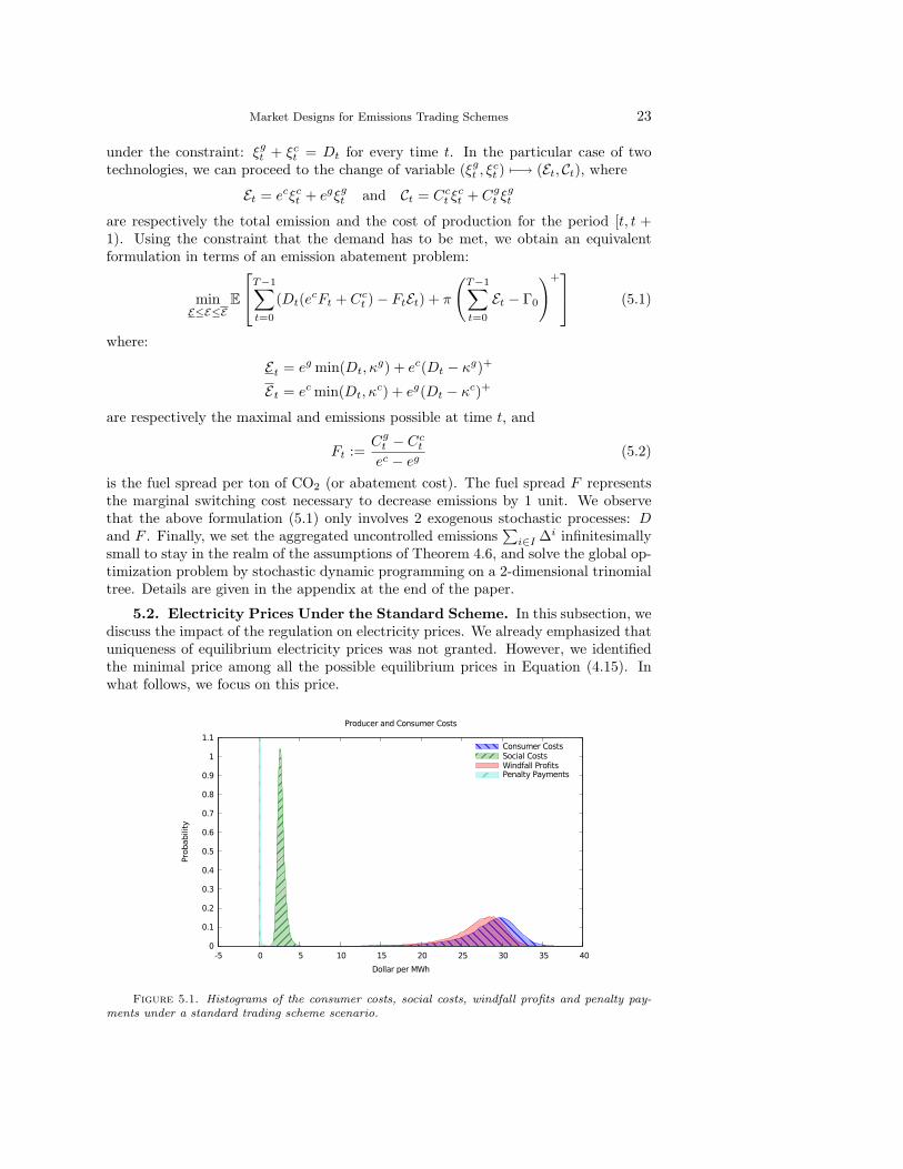


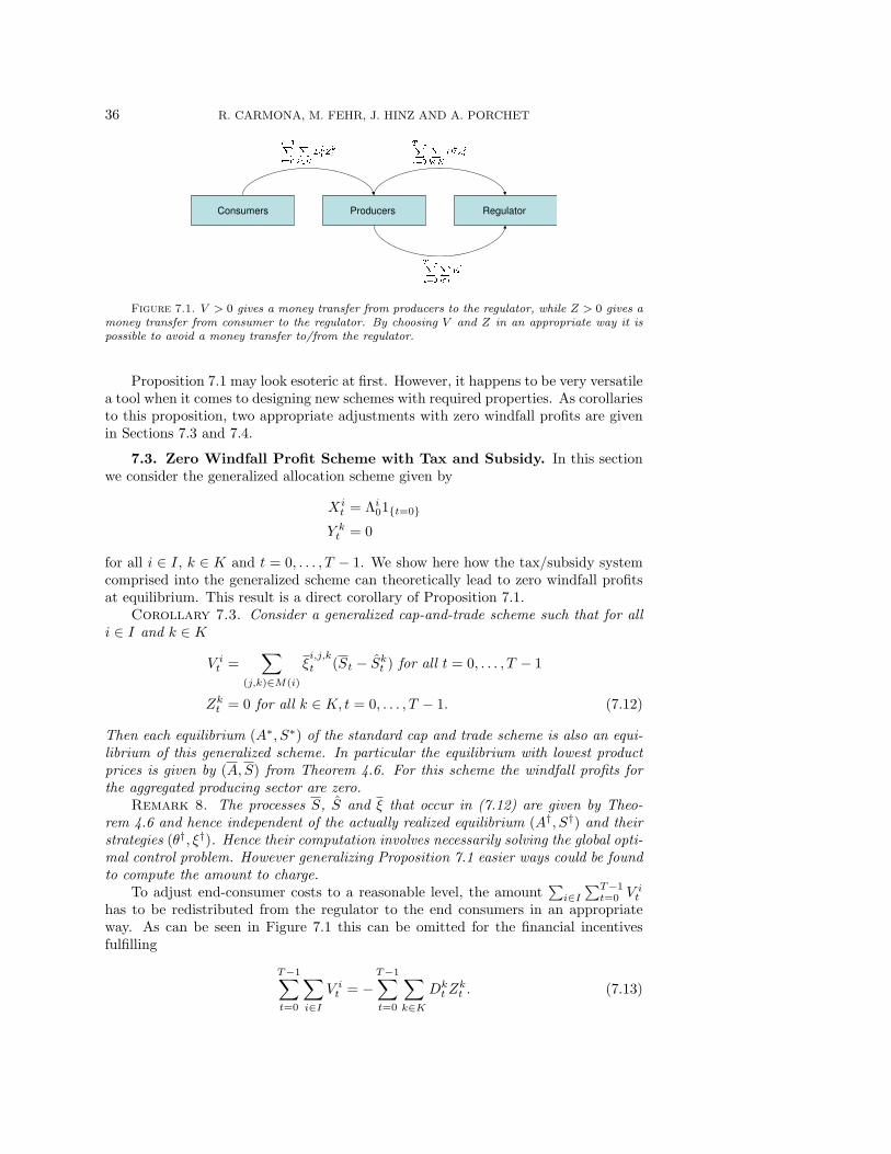


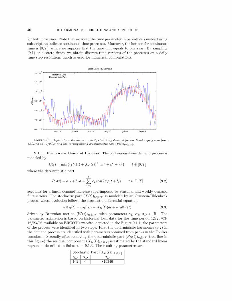
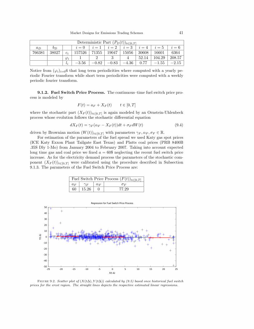


![Theory of single molecule emission spectroscopy...elaborate detection schemes have been developed to extend two-channel photon detection to mul-tiple channels [53] with an eye toward](https://static.documents.pub/doc/80x56/60c4c930edd75c37af736d64/theory-of-single-molecule-emission-spectroscopy-elaborate-detection-schemes.jpg)


