37
Market Fundamentals Frederick University 2012
| Date post: | 30-Dec-2015 |
| Category: |
Documents |
| Upload: | leslie-jenkins |
| View: | 213 times |
| Download: | 0 times |

Market Fundamentals
Frederick University
2012
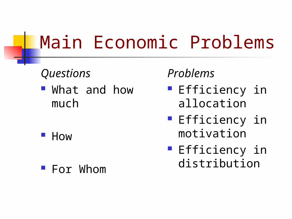
Main Economic Problems
Questions What and how
much
How
For Whom
Problems Efficiency in
allocation Efficiency in
motivation Efficiency in
distribution
Types of Economic Systems
Traditional economy Market Economy Command Economy

Market Functions
Allocation of scarce resources Motivation for efficiency Distribution of goods and services
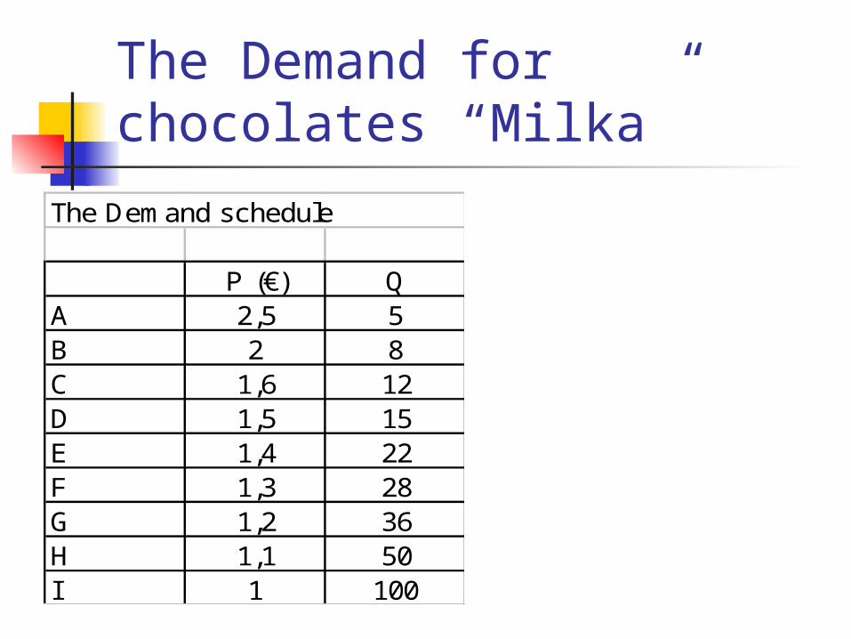
The Demand for chocolates “Milka”
The Demand schedule
P (€) QA 2,5 5B 2 8C 1,6 12D 1,5 15E 1,4 22F 1,3 28G 1,2 36H 1,1 50I 1 100
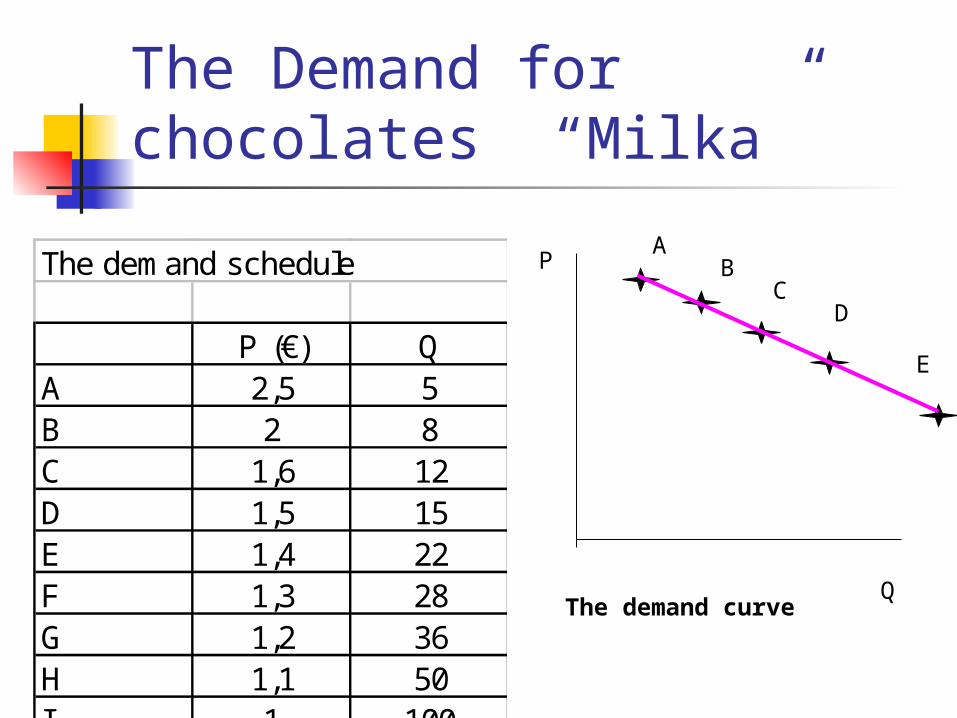
The Demand for chocolates “Milka”
The demand schedule
P (€) QA 2,5 5B 2 8C 1,6 12D 1,5 15E 1,4 22F 1,3 28G 1,2 36H 1,1 50I 1 100
P
Q
AB
CD
E
The demand curve
Demand
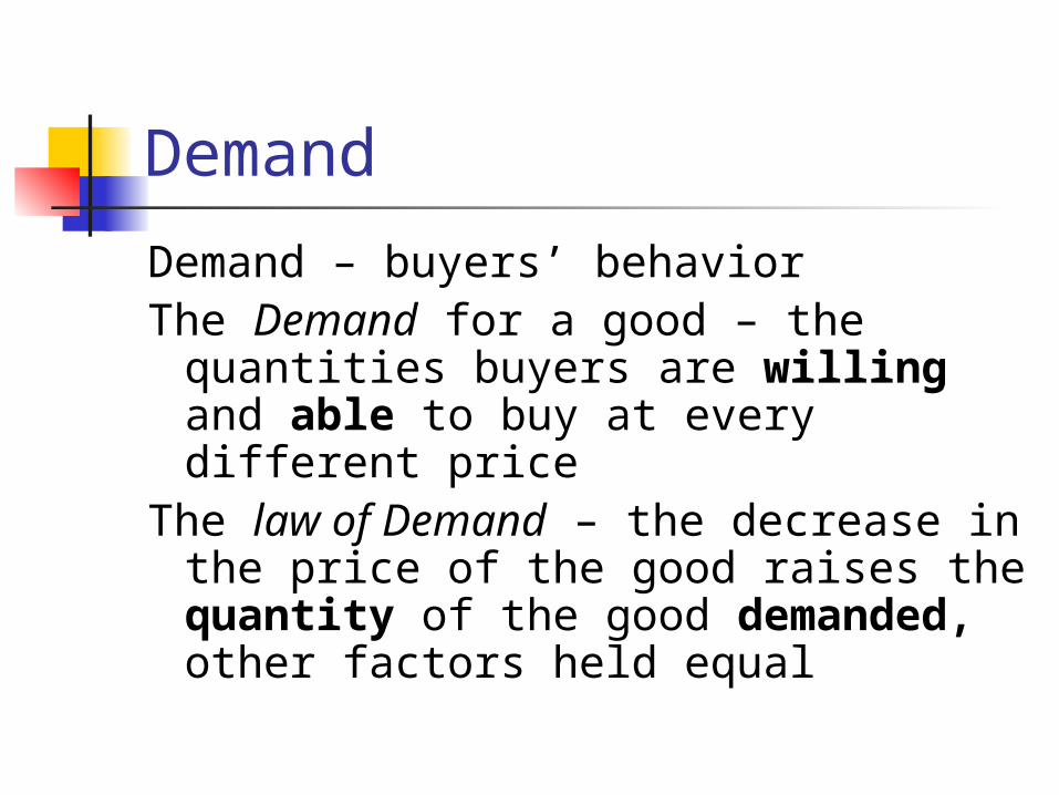
Demand – buyers’ behavior The Demand for a good – the
quantities buyers are willing and able to buy at every different price
The law of Demand – the decrease in the price of the good raises the quantity of the good demanded, other factors held equal

FACTORS DETERMINING DEMAND
Buyers’ income Prices of the other
goods Buyers’
expectations Buyers’ taste and preferences
Market size Institutions
P
Q
Demand rises = the demandcurve shifts rightwards
Demand falls = the demandcurve shifts leftwards
D
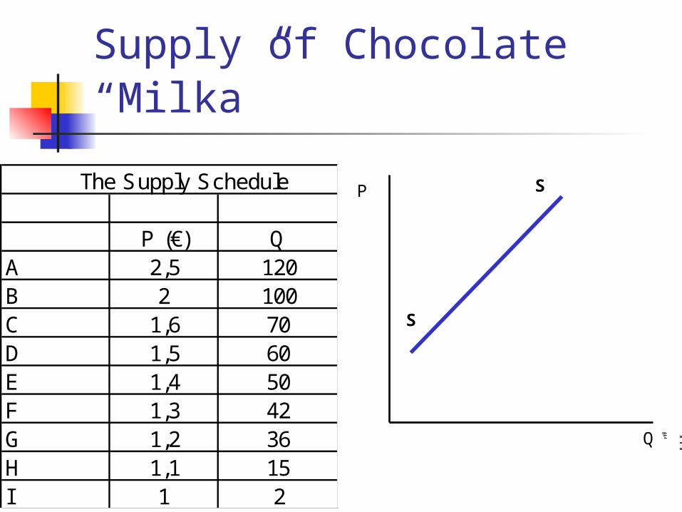
Supply of Chocolate “Milka”
050100
1st
Qt
r
East
West
North
The Supply Schedule
P (€) QA 2,5 120B 2 100C 1,6 70D 1,5 60E 1,4 50F 1,3 42G 1,2 36H 1,1 15I 1 2
P
Q
S
S
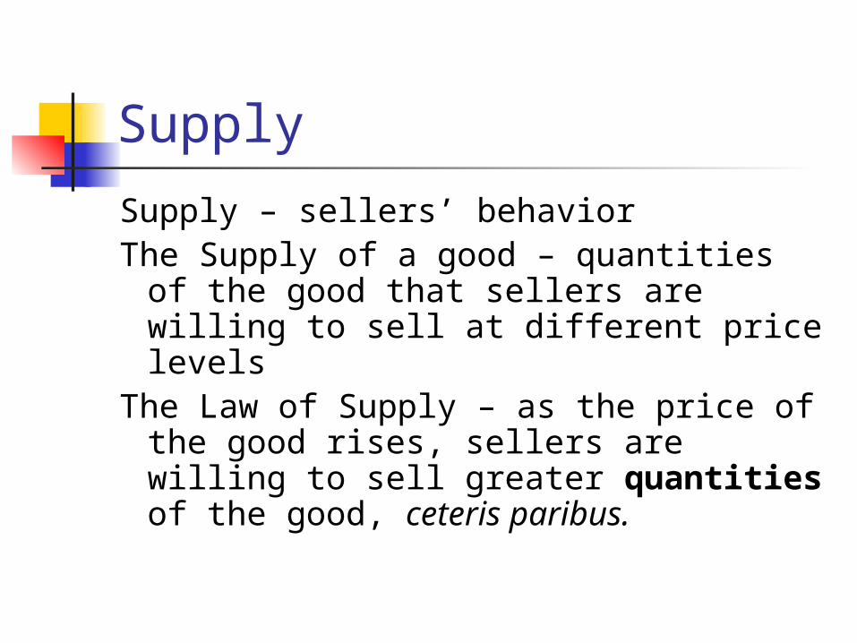
Supply
Supply – sellers’ behaviorThe Supply of a good – quantities of
the good that sellers are willing to sell at different price levels
The Law of Supply – as the price of the good rises, sellers are willing to sell greater quantities of the good, ceteris paribus.
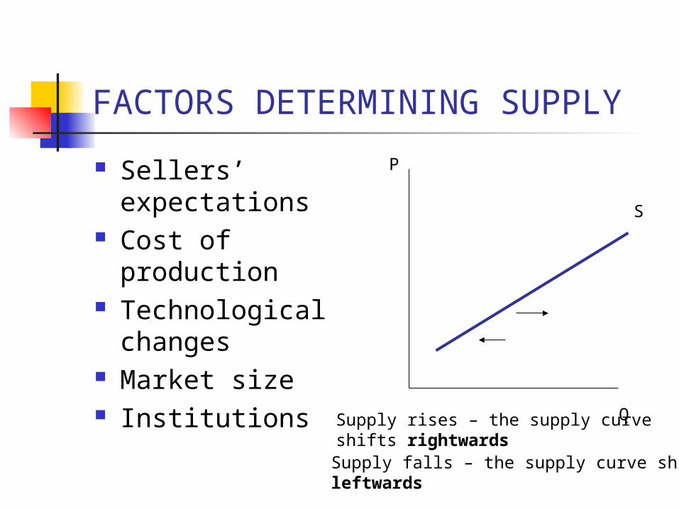
FACTORS DETERMINING SUPPLY
Sellers’ expectations
Cost of production Technological
changes Market size Institutions
P
Q
S
Supply rises – the supply curveshifts rightwardsSupply falls – the supply curve shiftsleftwards

Market Equilibrium
P
Q
D S
E
The market is in equilibrium when the quantity supplied equals the quantity demanded at the same price
Pe
Qe
The Supply Schedule
P (€) QA 2,5 120B 2 100C 1,6 70D 1,5 60E 1,4 50F 1,3 42G 1,2 36H 1,1 15I 1 2
The demand schedule
P (€) QA 2,5 5B 2 8C 1,6 12D 1,5 15E 1,4 22F 1,3 28G 1,2 36H 1,1 50I 1 100
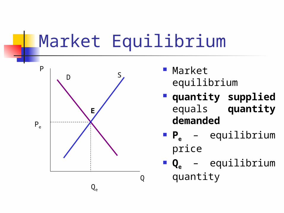
Market EquilibriumP Market equilibrium
quantity supplied equals quantity demanded
Pe – equilibrium price
Qe – equilibrium quantity
Q
D S
Pe
Qe
E
The Dynamics of Market EquilibriumP
Q
D
S
E
D’
Pe
Qe
Qd
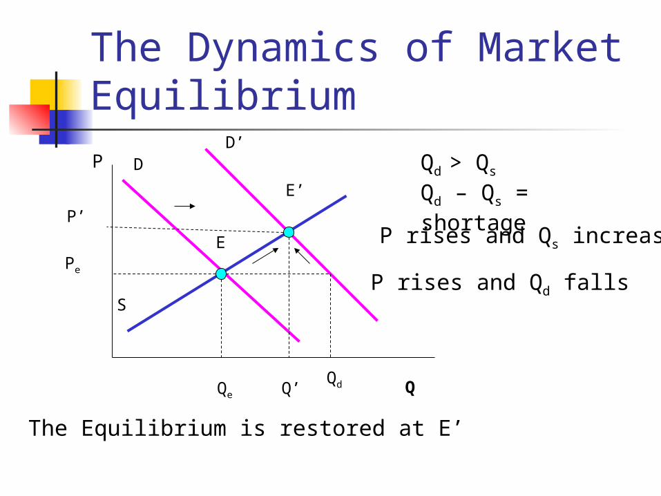
Qd > Qs
Qd – Qs = shortage
P rises and Qs increases
P rises and Qd falls
The Equilibrium is restored at E’
P’
Q’
E’
The Dynamics of Market EquilibriumP
Q
DS
EPe
Qe
S’
Qs
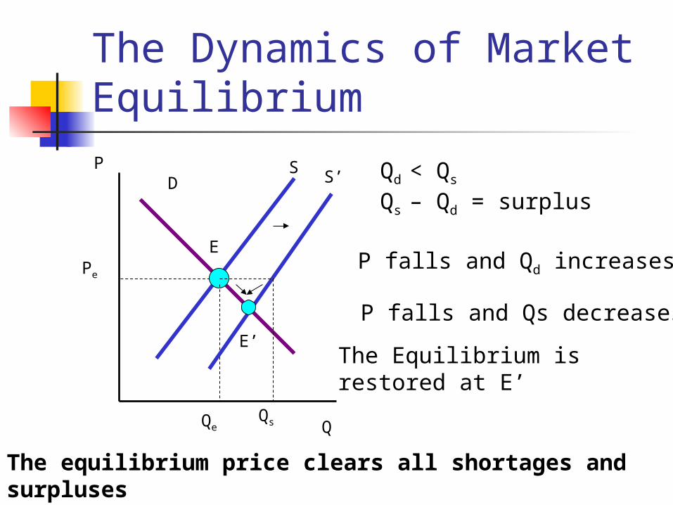
Qd < Qs
Qs – Qd = surplus
P falls and Qs decreases
P falls and Qd increases
E’The Equilibrium is restored at E’
The equilibrium price clears all shortages and surplusesPe = market clearing price
Price Ceiling
P
Q
D
S
Pe
Qe
Pc
Qs Qd
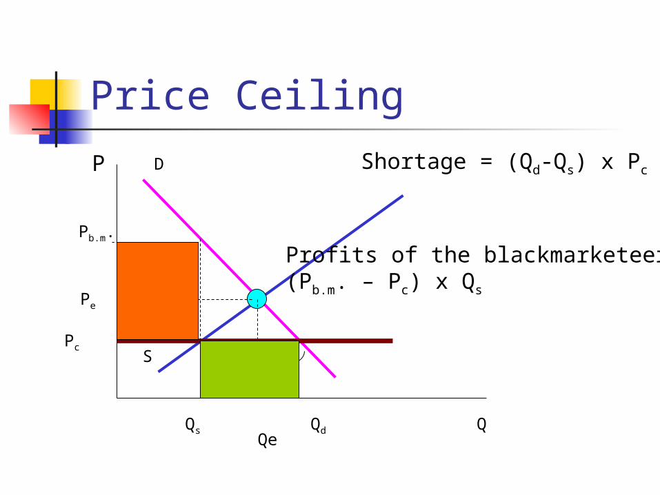
shortage
Pb.m.
Shortage = (Qd-Qs) x Pc
Profits of the blackmarketeers =(Pb.m. – Pc) x Qs

Arbitrage and speculationP
Q
Oz widget market
D
SPOz
QOz
P
Q
Zo widget market
D
S
PZo
QZo
Demand shifts to Zo marketSupply shifts to Oz market
Shifts in Supply and Demand until price differences are eliminated
exports
imports

Arbitrage and speculation
Arbitrage – the process by which individuals seek to make a profit by taking advantage of discrepancies among prices prevailing simultaneously in different markets
Speculation – a way to make a profit by taking a deliberately risky position
Quantifying Market Responses
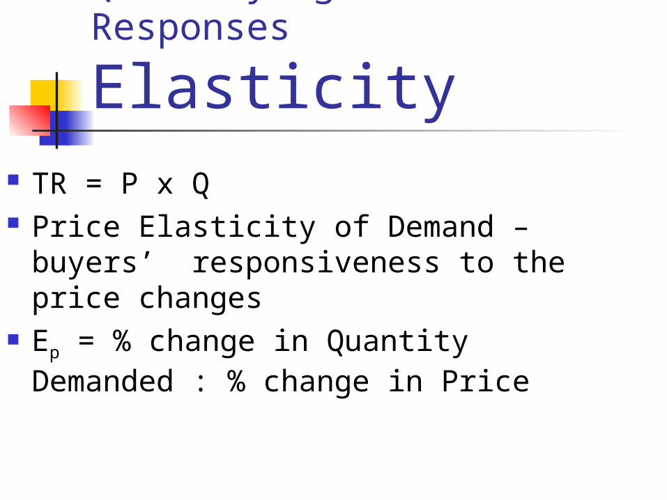
Elasticity TR = P x Q Price Elasticity of Demand – buyers’
responsiveness to the price changes Ep = % change in Quantity Demanded : %
change in Price
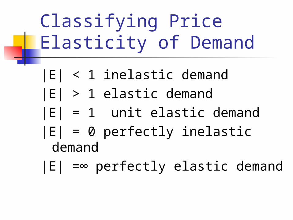
Classifying Price Elasticity of Demand
|Е| < 1 inelastic demand|E| > 1 elastic demand|E| = 1 unit elastic demand|E| = 0 perfectly inelastic demand|E| =∞ perfectly elastic demand
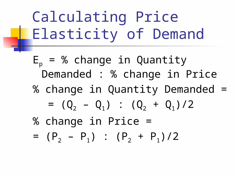
Calculating Price Elasticity of Demand
Ep = % change in Quantity Demanded : % change in Price
% change in Quantity Demanded = = (Q2 – Q1) : (Q2 + Q1)/2
% change in Price == (P2 – P1) : (P2 + P1)/2

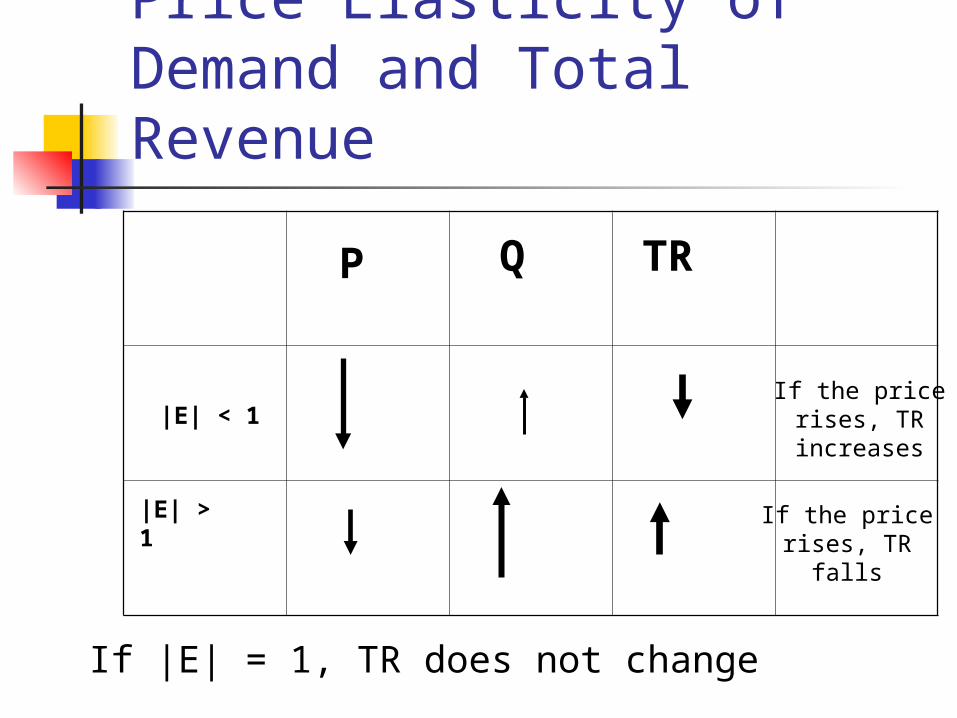
Price Elasticity of Demand and Total Revenue TR = P x Q The Law of Demand - If P rises, Q falls If the percentage change in price is
greater than the percentage change in quantity, the demand is inelastic
If the price falls, the change in quantity demanded does not compensate for the price reduction and TR falls
If the price rises, TR will increase
Price Elasticity of Demand and Total Revenue
P Q TR
|E| > 1
If the pricerises, TRincreases
If the pricerises, TR
falls
If |E| = 1, TR does not change
|E| < 1
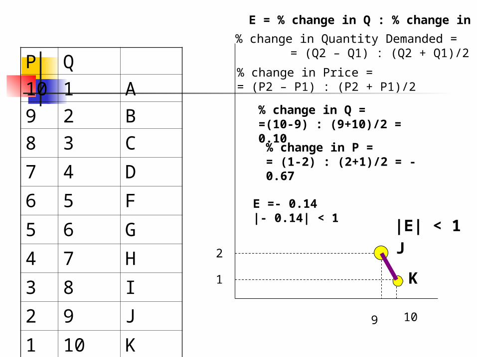
P Q
10 1 A
9 2 B
8 3 C
7 4 D
6 5 F
5 6 G
4 7 H
3 8 I
2 9 J
1 10 K
|E| < 1
2
9
1
10
E = % change in Q : % change in P
% change in Quantity Demanded = = (Q2 – Q1) : (Q2 + Q1)/2
% change in Price == (P2 – P1) : (P2 + P1)/2
% change in Q = =(10-9) : (9+10)/2 = 0.10% change in P = = (1-2) : (2+1)/2 = - 0.67
E =- 0.14|- 0.14| < 1
J
K

|E|>1
|E| < 1
|E|= 1
% change in Q = (6-5) : (6+5)/2 == 1.18
% change in P = (5-6) : (5+6)/2 = - 1.18
P Q
10 1 A
9 2 B
8 3 C
7 4 D
6 5 F
5 6 G
4 7 H
3 8 I
2 9 J
1 10 K
6
5
5
6
F
G
E = 1.18 : - 1.18 = -1|- 1| = 1
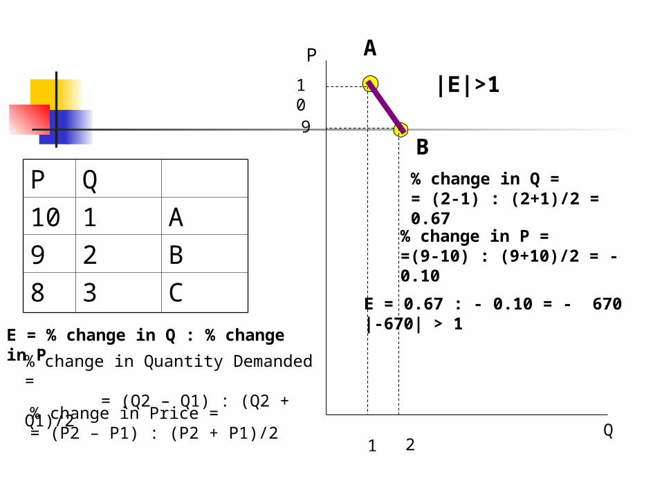
P Q
10 1 A
9 2 B
8 3 C
|E|>1
% change in Q = = (2-1) : (2+1)/2 = 0.67
% change in P = =(9-10) : (9+10)/2 = - 0.10
A
B
P
Q
10
1
9
2
E = % change in Q : % change in P
E = 0.67 : - 0.10 = - 670|-670| > 1
% change in Quantity Demanded = = (Q2 – Q1) : (Q2 + Q1)/2
% change in Price == (P2 – P1) : (P2 + P1)/2
FACTORS AFFECTING PRICE ELASTICITY OF DEMAND
Availability of substitutes/Definition of market
Time horizon Income Traditions

Price Elasticity of Supply
Price elasticity of supply – sellers’ responsiveness to the price changes
Ep = % change in Quantity Supplied : % change in Price

Price Elasticity of Supply
P
Q
E < 1
E > 1
E = 1
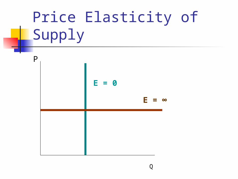
Price Elasticity of Supply
P
Q
E = 0
E = ∞

FACTORS AFFECTING PRICE ELASTICITY OF SUPPLY
Time horizon Availability of production factors Mobility of production factors Inventory levels Competitiveness of the market
structure Institutions
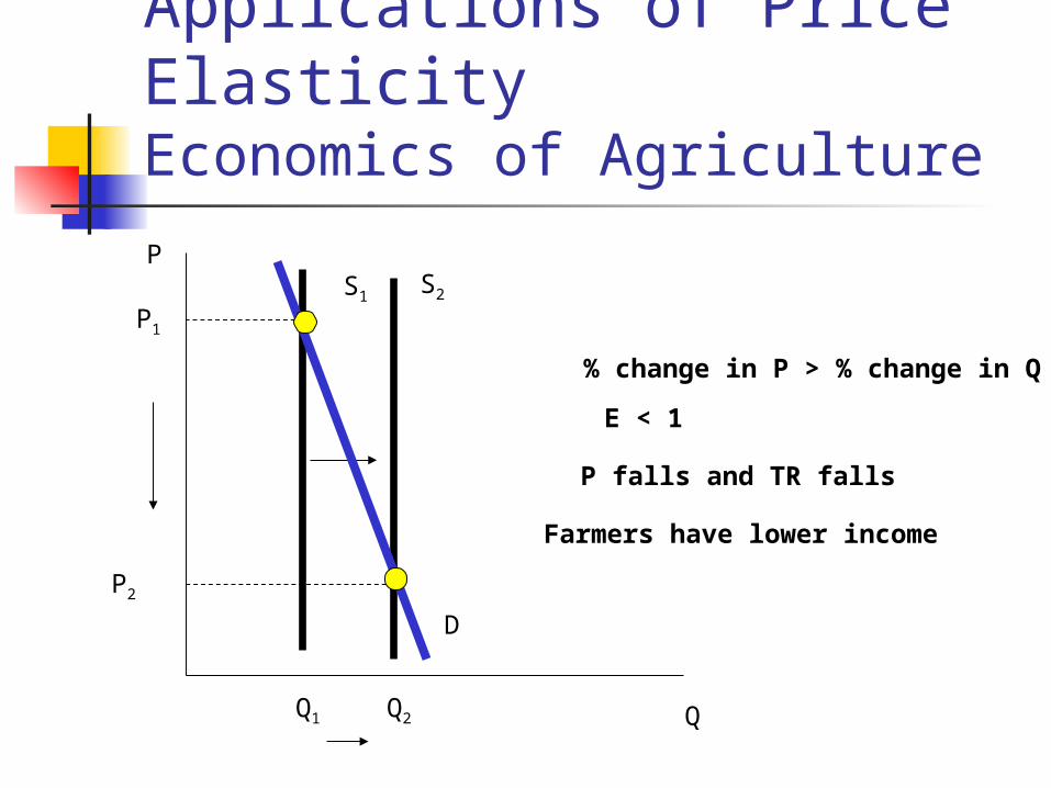
Applications of Price ElasticityEconomics of Agriculture
P
Q
S1 S2
D
Q1
P1
P2
Q2
% change in P > % change in Q
E < 1
P falls and TR falls
Farmers have lower income

Applications of Price ElasticityEconomics of Agriculture
P
Q
S
D
P1
P0
Q
Solution 1: government pays the difference P1 – P0 to the farmers
Government will lose (P1 – P0) x Q

Applications of Price ElasticityEconomics of Agriculture
P
Q
S
D
Q1
P1
P0
Q
Solution 2: government buys allQ from farmers at P1 and sells it.However, buyers will buy less at P1
Government cannot sell Q – Q1 and willlose (Q – Q1) x P1
Solution 2 is preferable because the loss is smaller.
The loss under solution 1 is (P1 – P0) x QThe loss under solution 2 is (Q – Q1) x P1
Since demand is inelastic, (P1 – P0) x Q > (Q – Q1) x P1
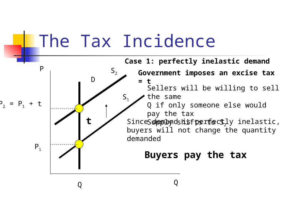
The Tax IncidenceP
Q
D
S1
Case 1: perfectly inelastic demand
Government imposes an excise tax = t
Sellers will be willing to sell the sameQ if only someone else would pay the taxSupply shifts to S2
Q
P1
Since demand is perfectly inelastic,buyers will not change the quantity demanded
t
S2
P2 = P1 + t
Buyers pay the tax
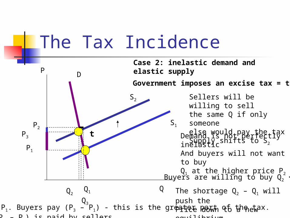
The Tax IncidenceP
Case 2: inelastic demand andelastic supply
Q
D
S1
Government imposes an excise tax = t
Sellers will be willing to sell the same Q if only someoneelse would pay the taxSupply shifts to S2
Demand is not perfectly inelastic And buyers will not want to buyQ1 at the higher price P2
Q1
P1
S2
P2
Buyers are willing to buy Q2 < Q1
Q2 The shortage Q2 – Q1 will push the Price down to a new equilibrium
P3 t
Q3Tax = P2 – P1. Buyers pay (P3 – P1) - this is the greater part of the tax. The rest (P2 – P3) is paid by sellers

The Tax Incidence
PCase 2: elastic demand andinelastic supply
Q
D
S1
Government imposes an excise tax = t
Sellers will be willing to sell the same Q if only someoneelse would pay the taxSupply shifts to S2
Demand is elastic And buyers will not want to buyQ1 at the higher price P2
Q1
P1
S2
P2
Buyers are willing to buy Q2 < Q1
Q2
The shortage Q2 – Q1 will push the Price down to a new equilibrium
P3
t
Q3
Tax = P2 – P1. Buyers pay (P3 – P1) - this is the smaller part of the tax. The rest (P2 – P3) is paid by sellers


