Market Liquidity Risk: Elusive no more

Market Liquidity Risk: Elusive No More Defining and quantifying market liquidity risk

Master’s thesis by: Kolja LoebnitzA

University of Twente Rabobank Group Utrecht, The Netherlands December 14, 2006

A [email protected]

mailto:[email protected]

Market L iquid i ty Risk: E lus ive no more Defining and quantifying market liquidity risk

Master’s Thesis by:

Kolja Loebnitz

Supervised by:

Klaroen KruidhofB

Rabobank Group

Berend RoordaC

University of Twente

Reinoud A. M. G. JoostenD

University of Twente

Utrecht, the Netherlands

December 14, 2006

B Klaroen Kruidhof, Group Risk Management – Balance Sheet Risk, Rabobank Group, [email protected] C Berend Roorda, PhD., Assistant Professor, FELab and Department of Finance and Accounting, University of Twente, [email protected] D Reinoud A. M. G. Joosten, PhD., Assistant Professor, FELab and Department of Finance and Accounting, University of Twente, [email protected]

Acknowledgments

This dissertation has benefited from the help of numerous people. In particular, I would like to

thank my supervisors Berend Roorda, Reinoud Joosten and Klaroen Kruidhof for their

comments and support. In addition, I am grateful to Kevin Filo, my sister Natascha, Paul

Finnie, Julia Garde and my family for their help.

"It is through science that we prove, but through intuition that we discover."

Henri Poincare, 1854 - 1912

Market Liquidity Risk: Elusive No More Defining and quantifying market liquidity risk

KOLJA LOEBNITZ

ABSTRACT

The concept of market liquidity risk has not been satisfactorily treated in

financial literature. Clear definitions as well as an understanding of the

phenomenon are lacking. This paper tries to change this by analyzing,

defining and measuring the phenomenon that is loosely termed market

liquidity risk. After representing a detailed intuitive framework, market

liquidity risk is defined as the perceived uncertainty regarding the

magnitude of the price concession(s) in excess of the expected value

required for an immediate transformation of an asset into cash or cash

into an asset under a specific trading strategy. Consequently we analyze

the usefulness of quantitative models to capture market liquidity risk for

the major asset markets. Finally, we suggest slightly adjusted versions

of the Almgren and Chriss (2000) and the Bangia et al. (1999) model.

Both models serve different purposes and may easily be implemented in

current risk measurement systems.

Market Liquidity Risk: Elusive No More 2

Management Summary Market liquidity risk has acquired a great deal of attention from researchers, regulators and financial institutions in recent times, as it is felt be to insufficiently covered by current risk management practices. With this work we attempt to contribute to a better understanding of market liquidity. Our research was commissioned to answer a range of questions relevant to a comprehensive review of the concepts of market liquidity and market liquidity risk, including:

What is a practical yet coherent definition of market liquidity and market liquidity risk? To what extent are current risk measures capturing market liquidity risk? To the extent that current risk measures are deemed insufficient, how should we quantify

market liquidity risk? We cannot claim to have answered all questions fully, but we do believe we have made important

contributions to the understanding of market liquidity. We have carried out the research in close consultations with the Group Risk Management department of Rabobank Group, however our research has been totally independent, and our arguments and conclusions are solely our own.

A proper definition of market liquidity and market liquidity risk is the central theme of our work. Most definitions found in literature fail in making the concept of market liquidity tangible. In our opinion a proper definition must allow for quantification in order to be valuable in practice. Most recommended definitions in literature do not fulfill that criterion and those few that do, lack other desirable features. For this reason we worked out our own definition based on a thorough analysis of frictions in financial markets, since most prior definitions, although inadequate in our opinion, suggest that frictions are at the heart of the topic of market liquidity.

We defined market liquidity as the discounted expected price concession required for an immediate transformation of an asset into cash or cash into an asset under a specific trading strategy. In other words, we defined market liquidity as the expected loss going from an asset to money or vice versa under a certain trading strategy. The value of the definition is twofold: (1) the definition can easily be formalized and (2) the definition reduces market liquidity to a single number in monetary units.

Accordingly we define market liquidity risk as the possibility that the price concession exceeds the expected value. That is to say, given a suitable model that specifies all the crucial variables such as a benchmark price, uncertain transaction costs and a trading strategy, we can employ well known risk measures such as Value at Risk or similar derivations to quantify market liquidity risk. However, for successfully applying the definition in practice we need suitable models. Given our definition it became evident that conventional market risk models do not capture the essence of market liquidity risk without significant modifications. Using our definition as reference point, we surveyed several quantitative methods that claimed to remedy some of the shortcomings of conventional models. As a result, we chose two models for different applications: (1) A model suggested by Almgren and Chriss (2000) that adequately quantifies the balancing act between price risk and uncertain transaction costs and (2) the Bangia et al. (1999) model that can be employed for portfolios of assets that do not require elaborated transaction costs formulations.

We conclude that with our definition one can finally formalize market liquidity and market liquidity risk and hence quantify both concepts. In practice the quantification of market liquidity risk might be hindered more by the lack of appropriate time-series than by model considerations. However, we highly recommend practitioners to address market liquidity risk and implement this new risk category into their current risk management systems. A failure to do so would leave most financial institutions exposed to significant undue risk. In addition, we recommend the integration of the concept of market liquidity risk into the broader framework of funding liquidity risk.


Contents in brief

PART 1: Trading Environment and Friction

1. Introduction 2. Friction 3. Trading Environment 4. Definition of Market Liquidity and Market Liquidity Risk 5. Financial Crises and Market Liquidity

PART 2: Modeling of Market Liquidity Risk

6. Quantification of Market Liquidity Risk

PART 3: Market Liquidity Analysis

7. Perspective of a Bank 8. Application in Practice

PART 4: Review and Closing Thoughts

9. Contribution 10. Outlook 11. Conclusions


Contents

Introduction........................................................................................................ 9 1.1 Topic ............................................................................................................................ 9 1.2 Relevance..................................................................................................................... 9 1.3 Objectives .................................................................................................................... 9 1.4 Structure...................................................................................................................... 9

Part 1 Trading Environment and Friction ............................................... 10

2. Friction ............................................................................................................................ 10 2.1 Lack of clarity ........................................................................................................... 10 2.2 Frictionless markets ................................................................................................. 10

3. Trading Environment .................................................................................................... 12 3.1 Trading ...................................................................................................................... 12 3.2 Types of markets....................................................................................................... 13 3.3 Trading process ........................................................................................................ 13 3.4 Types of orders ......................................................................................................... 14 3.5 Rules of precedence .................................................................................................. 14 3.6 Trading restrictions.................................................................................................. 15 3.7 Types of traders ........................................................................................................ 15 3.8 Transaction costs ...................................................................................................... 17 3.8.1 Bid-Ask spread....................................................................................................... 19 3.8.2 Price risk................................................................................................................. 24 3.8.3 Opportunity costs .................................................................................................. 28 3.8.4 Price impact costs .................................................................................................. 28 3.8.5 Magnitude of transaction costs............................................................................. 40 3.8.6 Minimizing transaction costs ................................................................................ 41 3.8.7 Requirements for the optimization problem....................................................... 42 3.9 Other asset markets.................................................................................................. 42 3.9.1 Fixed income market ............................................................................................. 42 3.9.2 Currency market ................................................................................................... 45 3.9.3 Option market........................................................................................................ 46 3.9.4 Futures market ...................................................................................................... 46 3.9.5 Bilateral negotiations............................................................................................. 47 3.9.6 Market overview .................................................................................................... 48 3.10 Friction revisited..................................................................................................... 49

4. Definition of Market Liquidity and Market Liquidity Risk ...................................... 50 4.1 Criteria ...................................................................................................................... 50 4.2 Survey and critique of available definitions........................................................... 50 4.2.1 Totality of characteristics ..................................................................................... 50 4.2.2 Diversity.................................................................................................................. 52 4.2.3 Expected conversion time ..................................................................................... 53 4.2.4 Expected price concession..................................................................................... 53 4.3 Definition of market liquidity.................................................................................. 55 4.4 Definition of market liquidity risk .......................................................................... 61


5. Financial Crises and Market Liquidity ........................................................................ 63 5.1 Definition and origins............................................................................................... 63 5.2 Diversity under attack .............................................................................................. 64 5.3 Conclusion ................................................................................................................. 67

Part 2 Modeling of Market Liquidity Risk................................................ 68

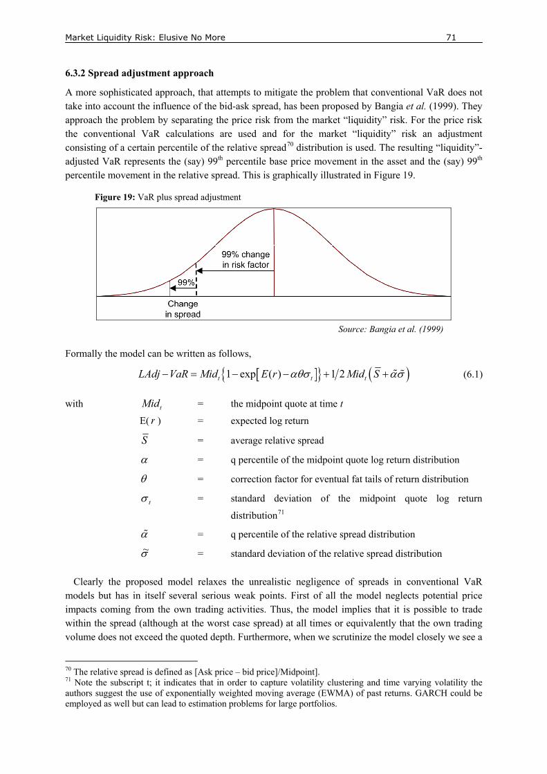
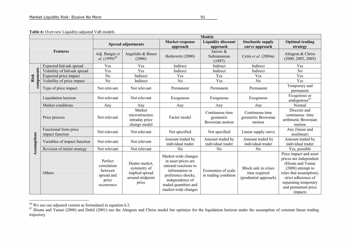
6. Quantification of Market Liquidity Risk .................................................................... 68 6.1 Objective.................................................................................................................... 68 6.2 Shortcomings of conventional VaR models............................................................ 68 6.3 Overview of existing approaches to quantify market liquidity risk .................... 70 6.3.1 Ad hoc approach.................................................................................................... 70 6.3.2 Spread adjustment approach ............................................................................... 71 6.3.3 Market price response approach ......................................................................... 73 6.3.4 Liquidity discount approach ................................................................................ 74 6.3.5 Stochastic supply curve approach........................................................................ 78 6.3.6 Optimal trading strategy approach ..................................................................... 80 6.4 Almgren and Chriss ................................................................................................. 81 6.4.1 Methodology........................................................................................................... 81 6.4.2 Price dynamics and impact functions .................................................................. 82 6.4.3 Total costs of trading............................................................................................. 83 6.4.4 Extensions............................................................................................................... 84 6.4.5 Specification of price impact functions................................................................ 84 6.4.6 Optimal trading trajectory for linear case .......................................................... 85 6.4.7 Liquidity-adjusted VaR ........................................................................................ 87 6.5 Synopsis ..................................................................................................................... 88 6.6 General applicability of the models ........................................................................ 90 6.7 Verdict ....................................................................................................................... 90

Part 3 Market Liquidity Analysis ............................................................... 93

7. Perspective of a Bank ..................................................................................................... 93 7.1 Funding liquidity versus market liquidity risk...................................................... 93 7.2 Market liquidity risk in banks................................................................................. 94

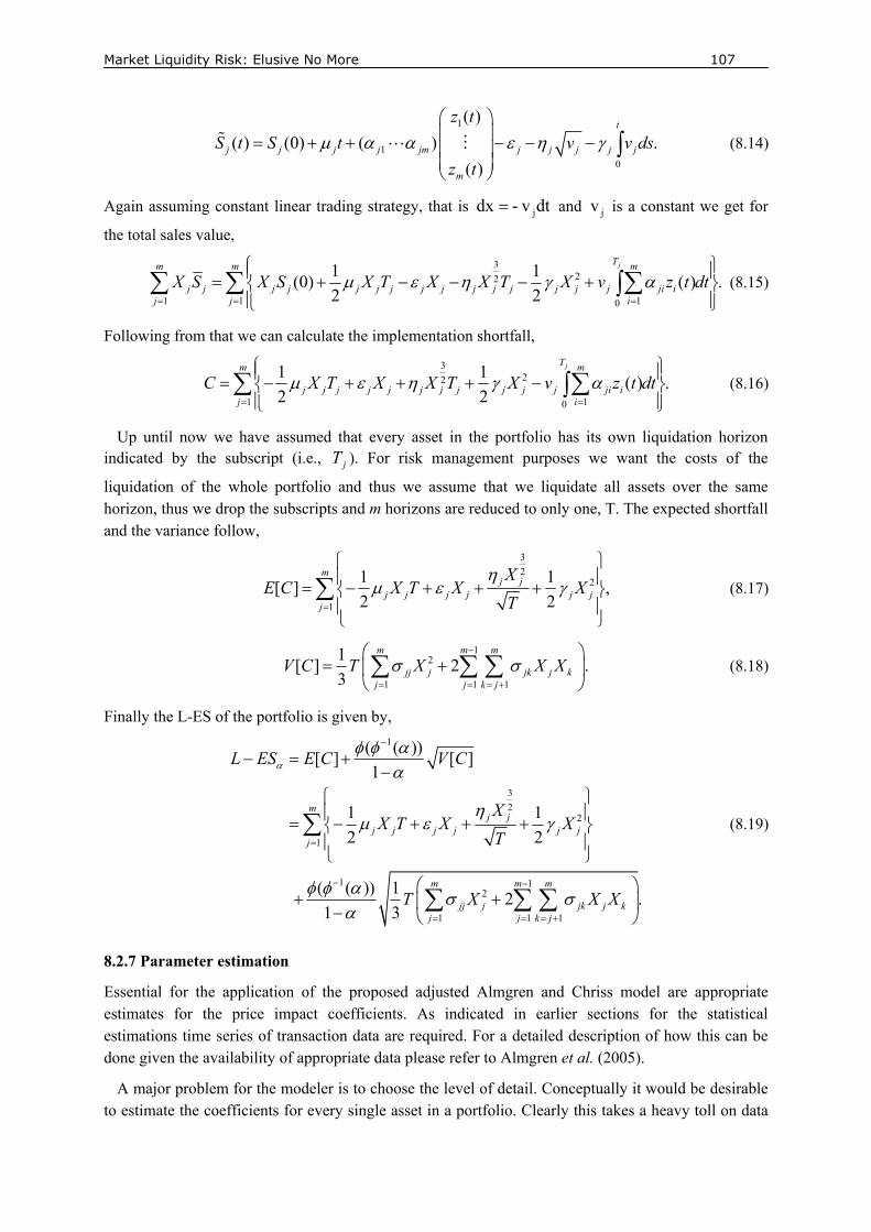
8. Application in Practice................................................................................................... 96 8.1 Objective .................................................................................................................... 96 8.2 Adjusted Almgren and Chriss model ..................................................................... 96 8.2.1 Continuous-time model ......................................................................................... 96 8.2.2 Price impact formulations .................................................................................... 98 8.2.3 Spectral risk measure............................................................................................ 99 8.2.4 Numerical examples ............................................................................................ 102 8.2.5 Sensitivity analysis............................................................................................... 103 8.2.6 Portfolio model..................................................................................................... 106 8.2.7 Parameter estimation .......................................................................................... 107 8.3 Adjustment VaR model for bond portfolios ........................................................ 108 8.4 Risk management and model risk......................................................................... 109 8.4.1 Problems in modern risk management.............................................................. 109 8.4.2 Model risk - Almgren and Chriss framework .................................................. 112 8.4.3 Model risk - Bangia et al. framework ................................................................ 114

Part 4 Review and Closing Thoughts .................................................... 115


9. Contribution ................................................................................................................. 115

10. Outlook – Research Suggestions ............................................................................... 115

11. Conclusions ................................................................................................................. 115

Appendix .......................................................................................................... 117 A1 – Coherent risk measure ........................................................................................ 117 A2 – Sensitivity analysis ............................................................................................... 118

References ........................................................................................................ 119


List of figures

Figure 1: Transaction costs.................................................................................................................... 19 Figure 2: Bid-Ask spread components .................................................................................................. 22 Figure 3: Quotation adjustments ........................................................................................................... 23 Figure 4: Delay in trading ..................................................................................................................... 25 Figure 5: Intra-day price risk................................................................................................................. 26 Figure 6: Price risk and price impacts ................................................................................................... 27 Figure 7: Effect of position size ............................................................................................................ 29 Figure 8: Post-trade price impact for a buy order.................................................................................. 30 Figure 9: Pre-trade price impact for a buy order ................................................................................... 30 Figure 10: Supply and demand curves .................................................................................................. 34 Figure 11: Price formation process ....................................................................................................... 35 Figure 12: Determinants of price impact............................................................................................... 37 Figure 13: Price impact functions ......................................................................................................... 38 Figure 14: Price impact costs for equities ............................................................................................. 40 Figure 15: Kyle's characteristics............................................................................................................ 51 Figure 16: Types of liquidity according to Neuman ............................................................................. 54 Figure 17: Vicious cycle of herding ...................................................................................................... 66 Figure 18: Illustration of different valuations methods ......................................................................... 70 Figure 19: VaR plus spread adjustment................................................................................................. 71 Figure 20: Illustration of price impact functions................................................................................... 83 Figure 21: Efficient frontier .................................................................................................................. 87 Figure 22: Trading strategy for various risk aversions.......................................................................... 87 Figure 23: Expected loss, 95% VaR and ES for an example loss distribution.................................... 101 Figure 24: VaR and L-VaR under different price impact specifications............................................. 103 Figure 25: ES and L-ES under different price impact specifications .................................................. 103


List of tables

Table 1: Main players and their trading motivations............................................................................. 12 Table 2: Tactics of dealers to manage inventories ................................................................................ 21 Table 3: Tactics of dealers to minimize damage after trading with informed traders ........................... 21 Table 4: Overview asset classes ............................................................................................................ 48 Table 5: Input parameters...................................................................................................................... 87 Table 6: Overview Liquidity-adjusted VaR models.............................................................................. 91 Table 7: Different price impact specifications ...................................................................................... 99 Table 8: Input parameters for numerical example............................................................................... 102 Table 9: Sensitivity analysis - holdings............................................................................................... 104 Table 10: Sensitivity analysis - time horizon ...................................................................................... 104 Table 11: Sensitivity analysis - temporary price impact coefficient ................................................... 105 Table 12: Sensitivity analysis - volatility of temporary price impact coefficient................................ 105 Table 13: Critical Almgren and Chriss model assumptions ................................................................ 114 Table 14: Sensitivity analysis - spread coefficient .............................................................................. 118 Table 15: Sensitivity analysis - permanent price impact coefficient................................................... 118 Table 16: Sensitivity analysis - correlation coefficient ....................................................................... 118


Introduction

1.1 Topic

This paper represents our effort to analyze, define and measure market liquidity risk. Although the term market liquidity risk is used quite readily in academic literature it lacks a clear definition, let alone understanding. This fact is recognized by many researchers as they mention the elusiveness of the phenomenon but nonetheless do nothing to change it. It is our hope that we change this unfortunate condition with our work.

1.2 Relevance

Risk management, as a standalone discipline, is a rather new invention and is most predominately found in the financial and insurance industry, for the main reason that risks are perceived to be more tangible and hence quantifiable. In addition, the sophistication of risk management is partially an answer to the ambitious agenda of regulators to foster bureaucratization of risk quantification in financial institutions and insurance companies. Regulators as well as corporations have established numerous categories that attempt to separate risks of different natures. Naturally for all parties involved it would be of outmost importance to know whether there is a risk type that has not been categorized and characterized. This is where this research comes in, as we try to clarify the essence of market liquidity risk, define it and suggest methods for its quantification.

1.3 Objectives

The objectives of this study can be summarized as follows:

1. Understand the essential aspects of market liquidity risk in the context of financial markets.

2. Derive a useful and coherent definition of this risk.

3. Establish a framework that allows the quantification of this risk.

We intentionally chose the starting point of our research to be of a fundamental nature as in our opinion this helps the reader to reproduce the line of reasoning that eventually lead to our conclusions. As a result, we hope this study provides a logical and precise treatment of the subject at hand that allows the reader to comprehend the problem step by step and not to leave the reader puzzled.

1.4 Structure

The dissertation is divided into four parts. The first part deals with the basic concepts and can be seen as the foundation for all our later enquiries. Particularly, we discuss the meaning of frictions in financial markets and explain its underlying processes. Most importantly, we analyze the key components of transaction costs in financial markets. The investigation on market frictions leads to the derivation of our definition of market liquidity and market liquidity risk. We conclude the first part by a concise discussion of the connection between financial crises and market liquidity. The second part deals with the quantification of market liquidity and market liquidity risk. We survey a range of quantitative models and choose in the end two appropriate models. In the third part we suggest slight modifications to these models to enhance the applicability in practice. Part four concludes.


Part 1 Trading Environment and Friction

In the first part we establish the foundation for all our later discussions by clearly differentiating essential concepts. We begin by choosing market frictions as an initial trail that could lead us to a meaningful definition of market liquidity and its inherent risk. As a guideline for this analysis we derive several open questions from the concept of frictionless markets. This leads us to a detailed description of the expansive trading environment of financial markets. We discuss types of markets, trading process, types of orders, rules of precedence, trading restrictions, types of traders and especially transaction costs. In the transaction cost section we analyze in detail bid-ask spreads, price impact costs and price risk. Next we suggest, relying on our prior results, a precise and practical definition of both, market liquidity and market liquidity risk. We conclude with a brief discussion of the link between financial crises and market liquidity. 2. Friction

2.1 Lack of clarity

Classical financial market theories are built upon the assumption of frictionless markets. However, this assumption does not apply for most markets (Çetin et al. (2004a)). Hence, market frictions, the absence of the price taking assumption and competitive markets, is the norm rather than the exception. Consequently, we could define friction in financial markets as the difficulty with which assets are traded (Stoll (2000)). Several authors came up with similar ways to define market liquidity. These definitions range from “…liquidity is the ease of trading a security” (Amihud et al. (2005)), “Liquidity risk…is defined as the risk of being unable to liquidate a position in a timely manner at a reasonable price” (Muranaga and Ohsawa (1998)) to “Market liquidity risk is the risk that a firm cannot easily offset or eliminate a position without significantly affecting the market price because of inadequate market depth or market disruption” (Bank of International Settlement (2006a)). At first sight these definitions seem to support the reader’s intuition but at a closer look the usefulness of those definitions disappear. The major flaw of all three definitions and basically the whole set of definitions for market liquidity1 is the vagueness of the terms used in the definition. Terms such as “ease”, “reasonable” and “timely” are empty without clarifications. The definitions fail the clarity of definition requirement2 and hence we have to reject these definitions.

Most previous definitions, although inadequate, suggest that frictions in financial markets are at the heart of the ambiguous concept of market liquidity and the market liquidity risk. Thus, it seems reasonable to start our research with an analysis of frictions in financial markets.

2.2 Frictionless markets

A good starting point for the analysis of friction in financial markets is the definition of what is considered to be a frictionless market. The characteristics of a frictionless market are that all traders

1 There are exceptions, which will be discussed in later sections. 2 The clarity requirement states that a definition should not allow double meanings and should not contain unknown and not understandable words/notions.


are price takers (any trader can buy or sell unlimited quantities of the relevant security without changing the security’s price) and that there are no transaction costs (including taxes) and no restrictions on trade (e.g., short sale constraints) (Çetin et al. (2004)). In other words, the law of one price should hold. The law is crucial in modern financial theory and says that instruments with identical future cash flows should have the exact same price as they are interchangeable and hence must have the same value. Let us dissect the meaning of this notion. First of all, the “all/any” implies that no matter what the characteristics of the trader or the desired trade are the price taken for the trade is the current market price and is not affected by any aspect of the transaction. Secondly, the notion implies that the sole expense borne by traders should be the market price for an asset. Finally, in a frictionless market there should be no regulations directly or indirectly limiting the trader’s inclinations to trade. As a guideline to analyze frictions and henceforth market liquidity we attempt to answer the following questions:

(1) Are there restrictions on trading?

(2) Are there transaction costs?

(3) Does any characteristic of the trader have an influence on price (to be) taken?

(4) Does any characteristic of the desired trade have an influence on the price (to be) taken?

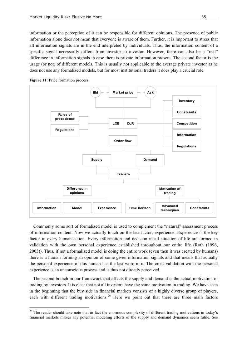
In order to find answers to the above questions we have to delve into what is called market microstructure literature. Market microstructure is the study of the process by which investors’ latent demands are ultimately translated into prices and volumes. Specific areas of interest include the price formation process, the influence of market structure and design on the efficiency of financial markets. We attempt to answer the questions in a systematic way by providing an overview of the key aspects of the trading environment, which entails information about the different market architectures as well as a discussion about transaction costs. Our discussion is principally applicable to all asset markets, although there is a slight bias towards equity markets mainly because more information are available. However, this bias is mitigated later on by analyzing the key differences between the major markets in terms of frictions.


3. Trading Environment

3.1 Trading

As was indicated, frictions in financial markets arise in the context of trading assets in a wider sense. Therefore, it seems appropriate to start our discussion with a global view on trading. It is common convention to distinguish between the buy side and the sell side of the trading industry. The buy side does not refer to actually standing on the buy side of every transaction but rather to buy exchange services. The exchange services are offered by the sell side. The most important service offered by the sell side is the ability to trade whenever the buy side intends to trade. In most cases, the buy side engages in trading3 to help solve numerous problems that originate outside of financial markets. Thus, trading in financial markets is used mainly as a tool. The buy side includes individuals, funds, companies and governments. Roughly one can categorize this diverse group of players in financial markets as investors, borrowers, hedgers, asset exchangers and gamblers.

Table 1: Main players and their trading motivations Trader type Examples Motivation Suited instruments Investors Individuals To move wealth from Stocks Corporate pension funds the present to the Bonds Insurance funds future for themselves Charitable and legal trusts or for their clients Endowments Mutual Funds Money managers Hedge Funds Borrowers Homeowners To move wealth from Mortgages Individuals the future to the Bonds Corporations present Notes Hedgers Farmers To reduce Future contracts Manufacturers uncertainties of future Forward contracts Miners developments Swaps Shippers Financial Institutions Asset exchangers International corporations Acquire assets that Currencies Manufacturers they value more than Commodities Travelers what they posses Gamblers Individuals Profit and

entertainment through Various volatile instruments

placing bets

Source: Harris (2003)

The group of investors engages in trading because they would like to transfer wealth from the present into the future either for themselves or more commonly for clients. Borrowers are keen on doing the opposite by transferring wealth from the future to the present. Hedgers would like to reduce their uncertainty about future developments through trading in various instruments. Asset exchangers intend to receive assets that they value higher than the assets they posses. Gamblers give bets to make profits and/or entertain themselves. Traders have a vast repertoire of trading instruments to choose from. Instruments include among other stocks, bonds, warrants, options, future contracts, forward contracts, foreign exchange contracts, swaps and commodities. Suitable trading instruments are chosen

3 Trading involves at least two parties and can be defined as the exchange of two instruments. Commonly trades involve the exchange of money against some other instrument but are not restricted to this.


by the traders depending on their objectives and motivations. For a summary of the classification of trader types and suitable trading instruments see Table 1 (Harris (2003)).

The sell side consists of dealers, brokers and broker-dealers. They provide exchange services to the buy side of the industry for money. Dealers stand ready to trade with their clients of the buy side to allow smooth trading activities. They earn profit when they can buy low and sell high. Brokers are agencies for their clients and trade on their behalf. They are paid to find other traders willing to act as counterparty for their client’s orders. Brokers earn commission fees for their services. In practice the functions of dealers and brokers are often combined. In those cases they are called broker-dealers (Harris (2003)).

3.2 Types of markets

The type of market refers to the way buyers and sellers are brought together so that assets can be transferred from one investor4 to another. Jain (2003) distinguishes between four types of markets: (1) dealer emphasis trading mechanisms (DLR), (2) pure electronic limit-order-book (LOB), (3) hybrid mechanisms (HYB) and (4) periodic call mechanism (CALL). In DLR markets dealers5 are obliged to stand ready to trade with investors at the bid and ask prices that they quote. Dealers trade on their own account and help that way to facilitate a steady market by providing immediacy even in the absence of natural buyers or sellers on the other side of the trade. In LOB markets there are no dealers. Instead all incoming orders are matched based on precedence rules (e.g., price and time priorities – see later sections). Those orders that cannot be matched are accumulated in a consolidated order book for subsequent matching. In HYB markets both DLR and LOB are used and hence the trading process is a combination of the two. In a CALL market orders are accumulated over a period of time and are then batch processed at a single price that would maximize volume. Pure CALL markets play a relatively insignificant role nowadays and hence we leave them out from our subsequent discussions (Jain (2003)). It has to be noted however that numerous exchanges such as the NYSE, are starting off a trading day with a call auction.

In the past most exchanges have relied on DLR markets but nowadays, primarily because of technological advances, over 80% of the exchanges in the world use some form of electronic trading mechanism with automatic execution (Jain (2003)). The most important exchanges in terms of volume use some sort of HYB (e.g., NYSE, NASDAQ, LSE and Deutsche Börse).

3.3 Trading process

According to Stoll (2001) it is useful to distinguish four main components evident in the trading process: (1) information, (2) order routing, (3) execution and (4) clearing and settlement. A major task of markets (i.e., exchanges) is to provide information about historical prices and quotes. Today most exchanges provide price information in real-time over consolidated trade systems and consolidated quote systems. The information allows traders to choose markets/exchanges with the best prices. Furthermore, they are input for all sorts of pricing and risk models employed by institutional investors.

Order routing is also a very important aspect of the trading process, as there are several ways an order can be processed. Let us say the investor has communicated the order to his broker. The broker

4 The terms investor and traders are used interchangeable throughout the text. Both refer to entities that engage in trading. 5 Throughout the text we use the term dealers, although there are various different names for essentially the same type of job, such as specialists, market makers, scalpers, day traders and locals. The terminology differs between exchanges and types of securities traded.


now has different choices depending on the type of order and his duty of “best execution”. Best execution in this case means that the broker has to evaluate the aggregated orders at some point in time and periodically asses, which competing markets, dealers, or electronic communications networks offer the most favorable terms of execution (Securities and Exchange Commission (2004)). Another option for brokers is to internalize the order. This means the order is filled out of the firm’s own inventory.

The execution is the most important step in the trading process and is subject to many studies in market microstructure. In principle we would expect that incoming market orders are matched with a resting quote. However, in a DLR market, dealers commonly refrain from executing a market order immediately in order to buy some time to assess potential presence of informed traders or “speedy” traders (Stoll (2001)). In LOB there are no dealers and the execution is based on precedence rules.

Clearing and settlement is the last phase and involves the comparison of transactions and the conclusion of the transaction, where the parties pay or get paid. The latter is called settlement and commonly it takes a couple of days (e.g., approximately three days in equity markets) until the bank accounts of both parties are actually credited/debited (Stoll (2001), NYSE Glossary).

3.4 Types of orders

Orders have three main aspects that define them: (1) order type, (2) execution conditions and (3) validity constraints. Generally one distinguishes between market orders and limit orders. A market order is a buy/sell order that is to be traded immediately at the best available price. A limit order is a buy/sell order that is to be executed at their specified limit or at a better price. In other words, if a trader files a limit order to buy, the limit order sets a maximum price that will be paid. In case of a limit order to sell the limit sets the minimum price that will be accepted.

The execution condition refers to whether an order should be executed in full or in part. The terms referring to the various order types differ between exchanges, but the ideas behind them are the same. For example, usually there are Immediate-or-cancel orders, which are order that are executed immediately and in full, or as fully as possible. The non-executed parts are not preserved as an order. There are also Fill-or-kill orders, which are orders that executed immediately and in full. Non-executed orders are deleted (Deutsche Börse (2003)). Other order types exist but shall not be discussed here.

The last aspect is the validity constraints, which determine how long the given order is valid. Three validity constraints shall be mentioned – good for day, good till date and good till cancelled (Deutsche Börse (2003)). Traders can beforehand specify how long the order should be valid in case the order is not executed immediately. This can be for a trading day, until a specified date or until it is cancelled (provided it does not reach a certain maximum age commonly specified by exchanges).

3.5 Rules of precedence

Rules of precedence determine the order by which orders are matched in all types of markets (DLR, LOB and HYB). Typically exchanges prescribe first priority to orders with the best price and secondary priority to the orders posted earlier at a given time. In some cases exchanges allow the secondary priority to be overwritten in the presence of large orders (Stoll (2001)). In other words, in some cases the larger order takes precedence over the smaller order although the smaller order was posted earlier at the same price. In DLR markets the dealers are obliged to follow the rules and in LOB markets a software algorithm is employed to enforce them.


Closely related to the precedence rules is the tick size of an exchange. The tick size is the minimum price variation allowed for orders (Stoll (2001)). The tick size can render the time priority rule useless if it is very small, since traders could try to increase the order by only one tick sin order to get precedence over earlier posted orders (Harris (1991)). This way they receive precedence.

3.6 Trading restrictions

Let us define trading restrictions as rules imposed by an authorized entity on traders and the trade that limit their expressions of will in terms of trading. The assumption of no trading restrictions in theory does not reflect the reality. In practice investors are faced by numerous rules and regulations that restrict their trading activities. We can distinguish between four categories of trading restrictions: (1) trading halts/circuit breakers, (2) collars, (3) margin requirements and (4) transaction taxes.

Circuit breakers or trading halts are rules enforced by exchanges to stop trading when the price of a certain benchmark index moved, or will most probably move, below (or less commonly above) a certain pre-specified level. The exchanges justify the implementation of circuit breakers by arguing that they provide investors with extra time to help them assess new information and make appropriate investment decisions during times of high market volatility (NYSE Glossary).

The second category of trading restrictions includes collars or also known as curbs. Again they come into effect when the price of a certain benchmark index moved below or above a certain pre-specified level. The collars entail limited access to computerized order submission systems and restrictions on filing of specific orders (e.g., index-arbitrage orders).

The next category of trade restrictions are margin requirements. Investors usually have the option to pay for the securities fully themselves or they may borrow part of the purchase price from their securities firm.6 When choosing to borrow part of the purchase price they have to open a margin account. The amount investors are required to deposit in a margin account before buying on margin or selling short is usually strictly regulated (e.g., in the Federal Reserve Board’s Regulation T for American markets). Some securities cannot be purchased on margin at all. In addition, most regulations stipulate minimum deposits at the beginning and certain maintenance requirements (NASD (2006)).

At last we have transaction taxes. Taxes on financial transactions are fees imposed by governments upon the sale, purchase, transfer or registration of a financial instrument (Wrobel (1996)). The tax characteristics vary considerably across countries. However, it is not important for our discussion to elaborate on these but only to recognize the existence of transaction taxes.

3.7 Types of traders

In literature there are various ways proposed to distinguish groups of investors. The most common way is to distinguish individual investors from institutional ones. Institutional investors are pension funds, banks, insurance companies, mutual funds, hedge funds, foundations and endowments. Those hold the majority of assets and usually trade in larger quantities (Stoll (2001)). For example, in 2002 institutional investors held approximately fifty percent of corporate equities, where American pension funds accounted for the largest chunk with more than twenty percent of total equity, followed by mutual funds and insurance companies (NYSE (2002)). In addition, Schwartz and Shapiro (1992)

6 Securities firms are equal to brokerage firms. Brokerage firms are simply the employers of brokers. Brokers act as agents on behalf of customers. Their job is to execute orders of their customers according to the best execution rule (this includes routing the orders)


underlined the importance of institutional investors by estimating that institutional investors accounted for approximately seventy percent of the total trading volume on the NYSE in 1989. There is no reason to believe that this is different in other asset markets. In many cases, it is assumed that institutional investors are better informed than individual investors because of their extensive research activities. This leads us to a second way of characterizing market participants.

Often authors distinguish between informed investors and liquidity traders. The liquidity traders trade because they want to account for their own consumption or to rebalance their portfolios to accommodate for desired changes in their risk profiles. In other words, liquidity traders buy assets if they posses excess resources or when they become less risk adverse. Similarly, they sell when they need resources or become more risk adverse (Stoll (2001)). The informed trader is said to possess private information about the value of an asset and tries to exploit on it through trading. Obviously, informed traders assume that the supposedly private information is eventually incorporated into the market price in such way as they believe it should. If we believe that this assumption is correct then a liquidity trader would lose against an informed trader when they trade with each other. The assumption of the presence of informed and liquidity traders and their trading with each other is the basis for numerous models employed in market microstructure literature (Stoll (2001)).

Harris (2003) proposes in the broadest sense the distinction between utilitarian and profit-motivated traders. Utilitarian traders trade to acquire some benefit other than trading profits whereas profit-motivated traders solely trade to achieve trade profits. Utilitarian traders are similar to the players of the buy side we discussed in the beginning only that we add fledglings, cross-subsidizers and tax avoiders. Fledglings trade in order to learn how to trade, cross-subsidizers trade to transfer wealth to other people in order to acquire specific services in return (i.e., “soft dollars”) and tax avoiders trade to minimize their taxes by exploiting tax loopholes.

Harris (2003) identifies three distinct classes of profit-motivated traders: (1) informed traders, (2) order anticipators and (3) bluffers. Informed traders acquire information about the fundamental value of a security and then attempt to take advantage on it if the market value differs from their own estimates. Commonly in literature informed traders are assumed to possess private information, information that is not available to the public. According to Harris (2003), the category of informed traders includes value traders, news traders, information-oriented technical traders and arbitrageurs. Value traders perform fundamental analyses of assets, which involve collecting as much information as possible that could tell them something about the fundamental value of a security. Then usually, applying some sort of economic model to organize and evaluate the information, they arrive at an estimate for the value. Having done so they arrive at overvalued and undervalued securities by comparing the value they derived and the market value. Accordingly, overvalued securities are then shorted and undervalued securities are bought. News traders try to benefit from forecasting the direction of market prices caused by arrival of new material information.7 Technical traders or chartists try to take advantage of recurring price patterns. Arbitrageurs try to exploit inconsistencies in pricing of securities relative to each other. If such inconsistency is identified the arbitrageurs buy the supposedly cheaper instrument and sell the supposedly more expensive ones in the hope that the inconsistency dissolves.

The second category involves order anticipators. Those are traders who hope to profit from trading before other traders trade. The key to their success is to anticipate the trade intentions of other traders

7 Economists distinguish between material and stale information. Material information are information that will significantly affect market prices. Stale information on the other hand are already incorporated in prices.


and the effect on the price. Order anticipators are also called stealth or parasite traders as they only profit when they prey on other traders. Within the category of order anticipators we have front runners, sentiment-oriented technical traders and squeezers. Front runners try to gather information regarding trades other traders are planning to execute and then try to trade before (in front) them in order to benefit from potential price movements induced by the trades. Sentiment-oriented technical traders attempt to predict trades of uninformed traders and then exploit potential price movements triggered by them. Squeezers attempt to corner the market. In other words, they try to monopolize one side of a market, so that everyone who is willing to trade must negotiate with them. If that strategy is successful the squeezers can demand almost any price. Squeezes are mostly illegal nowadays.

The last group of traders according to Harris (2003) consists of bluffers. Bluffers try to trick other traders into unwise trades they profit from. There are two types of bluffers, rumormongers and price manipulators. Rumormongers attempt to spread information that convinces other traders to trade in a certain way that would benefit the bluffers. The information can be either completely false or correct but misrepresented information. Price manipulators precisely arrange their own trades in such a way that other traders change their opinion of the value of the traded instrument. In most countries rumormongers and price manipulations are illegal although in most cases it is hard to prove malicious intent.

We mentioned that liquidity traders or similarly institutional investors are commonly managing their portfolios, which are subject to risk profile adjustments and consumption changes. We should further mention the importance of hedging positions using the underlying assets, diversification as well as the role played by hedge funds. The reason why we stress the role of hedging, diversification and hedge funds is that the motivation for trading can be quite different to the motivations used by other traders.

As will become clear in later sections registered dealers are a special type of traders that play a crucial role in financial markets. Dealers can be classified as the ultimate liquidity traders as they are obliged by the exchanges, where they are registered, to enable a fair and orderly market. That means that they have to stand ready to buy and sell at their own quoted prices with other traders on their own account.

3.8 Transaction costs

Transaction costs include all costs that can be attributed to a transaction. This seems straightforward but actually it is not. The problem starts in defining the boundaries of the concept of a transaction. In other words, which dimensions and to what extent do we include them into our definition. Let us take for example the time dimension. We could define the starting point of a transaction as the point in time where the trader forms his intention to execute a certain trade (sell or buy a specific amount of an asset) for some specific reason or we could use the point in time when he actually communicates the order. Similarly, what happens when the trader decides to sell a large position in numerous smaller parts? Should this be considered as one transaction or several?

Let us start by agreeing on the time dimension of a transaction. We define the moment a transaction comes into existence when the order is communicated by the trader to the responsible entity.8 The entity can be a broker or an electronic communication network. It is not important who the entity is only that the order is processed / documented. It is worth to note that the starting point of a transaction must be an a posteriori concept as it implies that a transaction has actually taken place after the

8 We restrict our discussions on organized exchanges for now. Over the counter (OTC) markets will be analyzed in later sections.


starting point. Of course not all orders that are placed result in transactions (e.g., the limit of a limit order is reached or validity constraints are hit).

Now that we have defined the starting point we need to consider the point in time when the transaction ends. Let us define the end of a transaction when a willing counterparty is found and the transaction price is fixed. Now we can analyze all the costs that a trader incurs in this specific time interval and that can be associated with the transaction. We define the costs associated with a transaction to be the costs that arise during the earlier defined time interval and that would not incur if not because of the transaction. Note that this definition includes potential opportunity costs. Our definition is in line with most authors but some do not explicitly include the time dimension as we do (see, for example, Bervas (2006)).

Having defined transaction costs we can now analyze what type of costs traders in practice encounter. For illustrative purposes we try to assign the types of costs to the time interval defined early. Commonly there is a distinction made between explicit and implicit transaction costs. Explicit transaction costs are usually associated directly with the communication of the desired order (e.g., fees, taxes) whereas implicit costs are usually seen as all costs that do not fulfill this criterion but can still be associated with the transaction. In our opinion it is more useful to distinguish between certain and uncertain transaction costs (see Figure 1 for an overview). As defined before the starting point of a transaction is the communication of the desired order9 by the trader to the responsible entity. When the order is filed via a broker commission fees are charged. Similarly, fees have to be paid after a transaction in organized markets to the exchange as well as to the government in the form of taxes. It is plausible to assume that these fees are static and hence are known by the trader before the order was placed. In others words, commissions, fees and taxes are certain transaction costs. After the processing the order is communicated to the market. The order is then either executed almost instantly or put in the “waiting line”, depending on the order size and the demands of the market.

We can identify four types of costs that are uncertain to the trader before the transaction: (1) bid-ask spread, (2) price risk, (3) opportunity costs and (4) price impact. The difference between the midpoint quote price and the bid or ask price, depending on the sign of the order, can be seen as a cost for the trader. The bid-ask spread and hence the difference is not static. Dealers have good reasons to adjust their quoted bid and ask prices throughout the day as will be discussed in the next section. Price risk arises as traders might experience adverse price movements between the processing of the order and the execution. As we have mentioned it is very well possible that it takes a certain amount of time to execute an order, which is not constant and hence uncertain. Price risk in the contents of transactions clearly increases the larger the time interval gets and becomes very important when a trader opts for splitting up a large order into smaller parts and distributes them over time.

9 The order always states the desired asset, the direction (buy or sale) and the amount, whereas the statement of the desired price depends on the type of order placed (e.g., market order, limit order etc.). In addition one must include the execution conditions and the validity constraints.


Figure 1: Transaction costs

TaxesFees OpportunitycostsPrice risk

Transactioncosts

Certain Uncertain

Commissions Bid-Ask spread Price impactcosts

Closely related to price risk are opportunity costs. Generally opportunity cost, also referred to as economic cost, is the value of the best alternative that was not chosen in order to pursue the current endeavor, i.e., what could have been accomplished with the resources expended in the undertaking. Thus, it represents opportunities forgone. In case of transaction costs the time delay in trading determines the magnitude of the opportunity costs. The opportunity costs are uncertain because of the random length of the time interval.

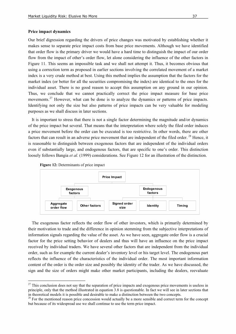
Price impact costs refer to adverse price movements caused by the desired trade itself. Commonly it is measured as the difference between a benchmark and the actual transaction price. The benchmark price is typically the midpoint quote just before the order is processed. One can imagine that it is difficult to distinguish between the factors causing adverse price movements. Thus, isolating the effective price impact costs is not easy. The underlying assumption for determining the price impact costs, by taking the differences between a benchmark and the actual transaction price, is that the filed order is solely causing the adverse movement of the transaction price. For the practitioner it does not matter so much what caused the adverse change in the transaction price but for our discussion it might be interesting to entangle the various factors.

3.8.1 Bid-Ask spread

As has been discussed before there are DLR markets and LOB markets (and HYB markets). Because of their different market structure the matching procedures are different as well. In the past there were no LOB markets as the technology was not sophisticated enough. This has changed dramatically as there is a great number of exchanges that adopted LOB mechanisms.10 As a result, we have to look at both forms of markets separately in terms of the quoting process and the bid-ask spread.

Dealer markets

Generally there is a difference between the price an investor gets when he wants to sell an asset and the price he has to pay when he wants to buy an asset. The price he has to pay to buy an asset is the ask price and the price he gets when he sells an asset is the bid price. The ask-price is always larger than the bid-price. The difference between the buy (ask) and the sell price (bid) can be explained by the presence of dealers. The difference between the bid price and the ask price is the margin for the dealers. Recall that dealers ensure that there is always a market in which investors can buy and sell assets. Basically these persons make the markets (a market can be defined by its main function,

10 Among other - Equities: NYSE’s OpenBook program, Nasdaq’s SuperMontage, Toronto Stock Exchange, Vancouver Stock Exchange, Euronext (Paris, Amsterdam, Brussels), London Stock Exchange, Copenhagen Stock Exchange, Deutsche Börse, and Electronic Communication Networks such as Island. Fixed income market: eSpeed, Euro MTS, BondLink and BondNet. Derivatives market: Eurex, Globex, and Matif (Obizhaeva and Wang (2005)).


namely to bring buyers and sellers together in whatever way). Clearly, dealers in financial markets do not differ in principle from dealers in non-financial areas, as sorts of dealers make profit by buying at low prices and selling at higher prices. Generally exchanges officially register traders as dealers. This way the dealers receive some privileges and in turn are required to enable trading (i.e., continuously providing quotes to the market).11

Dealers are usually required by the exchanges to quote a two-sided market that is to quote both a bid and ask prices. The quotes of dealers can either be firm or soft. Firm quotes require dealers to trade at their quoted prices if traders wish so, whereas soft quotes simply indicate potential interests and can be changed by dealers or completely taken back when traders actually desire to file orders. Registered dealers are usually required to post firm quotes. In some markets dealers quote prices only on request, which then expire after a pre-specified time. As there are commonly several dealers there are several different spreads available. The inside spread is the difference between the highest bid price and the lowest ask price available in the market, where both quotes do not necessarily belong to a single dealer. In addition to quoting bid and ask prices dealers also quote bid and ask sizes, which are the maximum quantities they are willing to trade at the quoted prices. The prices at which trades execute are often not the same as the previously quoted prices. The actual spreads realized by the dealer are called effective spreads. What is commonly known as the market price is the average of the best bid and the best ask price, that is the midpoint of the inside spread.12 From the description of the job of the dealer two things are obvious: first, dealers need extensive order flow to make profit, and second, dealers in financial markets face risks, as they do not know beforehand at what price and to whom they can sell a security after they make a purchase on their own accounts. The main way to attract order flow is by quoting aggressive prices. Another way is to build close relationships with clients, i.e., brokers and institutional investors, by providing them with market information and sometimes by entertaining them through diners and popular sport events. The quoting decision at any given time is complex for the dealers (Harris (2003)). The prices dealers quote are driven by two problems: (1) inventory control and (2) dealing with informed traders. By quoting firm prices and trading with investors, dealers accumulate inventories. Inventories increase when dealers buy at the bid price and decrease when they sell at the ask price. Because dealers are passive traders (i.e., they trade when other want to trade) inventory levels are determined mainly by fluctuations in the demands of traders. Since dealers usually have target inventory levels, they try to attract signed order flow in such a way that they reach those levels.13 They do that through posting attractive prices and bid-ask sizes. A summary of potential tactics that can be employed by dealers can be found in Table 2.

11 More specifically there are two main rules governing the trading of registered dealers at organized exchanges: (1) affirmative obligations (provision of continuous quotes) and (2) negative obligations (restriction of own trading). The major privilege that comes from being a registered dealer is the ability to access the entire system order flow before anyone else can (Harris (2003)). In OTC markets such regulations are usually nonexistent or very limited. 12 Sometimes the market price is also the transaction price of the last trade. We will refer to the market price as the midpoint quote of the inside spread as it is more commonly used. 13 Not all dealers have the same target inventory, but generally when short positions are as expensive to create and hold as long positions and dealers are not speculating, hedging or investing for themselves, then the target inventory is zero. If either of the two assumptions are not met target inventory levels are different (Harris (2003)).


Table 2: Tactics of dealers to manage inventories Condition Tactic Purpose

Raise bid price Increase bid size

Encourage clients to sell

Raise ask price Decrease ask size

Discourage clients from buying

Take another dealer’s offer (buy at another dealer’s ask price)

Immediately raise inventories Inventories are too low

Buy a correlated instrument Hedge the inventory risk Lower ask prices Increase ask size

Encourage clients to buy

Lower bid price Decrease bid size

Discourage clients from selling

Hit another dealer’s bid (sell at another dealer’s bid price)

Immediately lower inventories Inventories are too high

Sell a correlated instrument Hedge the inventory risk Source: Harris (2003)

The second factor influencing the price quoting decision of dealers is the risk of dealing with informed traders. As discussed before informed traders are assumed to have knowledge of future price movements of securities. In that case dealers tend to lose when trading with informed traders as they cannot buy low and sell high anymore, because of subsequent adverse price movements. However, dealers have certain tactics to minimize damages when they suspect that they have traded with informed traders. See Table 3 for a summary.

Table 3: Tactics of dealers to minimize damage after trading with informed traders Suspected Condition Tactic Purpose

Raise ask price Lower ask size

Discourage further sales to informed traders

Raise bid price Raise bid size

Encourage clients to buy quickly and thereby restore inventory position before prices rise

Take another dealer’s offer (buy at another dealer’s ask price)

Quickly restore target inventory; this strategy pays for immediacy, but the cost may be less than the loss that will result if prices rise while the dealer is short

Sold to an informed trader

Buy a correlated instrument Hedge the inventory risk and speculate on information

Lower bid prices Lower bid size

Discourage further purchases from informed traders

Lower bid price Raise bid size

Encourage clients to sell quickly and thereby restore inventory position before prices fall

Hit another dealer’s bid (sell at another dealer’s bid price)

Quickly restore target inventory; this strategy pays for immediacy, but the cost may be less than the loss that will result if prices drop while the dealer is long

Bought from an informed trader

Sell a correlated instrument Hedge the inventory risk and speculate on information


The tactics and elements discussed so far are intuitively convincing and are based on practical considerations. However, it might be interesting to see the results of empirical and theoretical studies. Generally the practical and theoretical analyses agree. There are two streams of explanations found in


literature of why there are bid-ask spreads. The spread reflects (1) a compensation for the immediacy service of dealers or (2) the redistribution of wealth from some traders to others (Stoll (2000)). According to the first view compensation for immediacy encompasses a payment for the real economic resources required by dealers to do their job (e.g., labor and capital required to execute orders, clear and settle orders etc.), demand pressure and potentially monopoly rents (increases of the spread relative to costs because of market power). Papers discussing this approach include Garman (1976), Stoll (1978), Amihud and Mendelson (1980), Cohen et al. (1981), Ho and Stoll (1981, 1983) and Laux (1995). The second view tries to explain the spread by an informational argument. Either by way of asymmetric information among market participants, or by arguing that the dealer effectively grants an option to investors for free, where the option entails that in case new information arrives before the dealer can adjust the quote he loses to a “speedy” investor. The asymmetric information view explains the spread as a compensation for losses incurred by trading with informed investors. Papers discussing the informational view include Bagehot (1971), Copeland and Galai (1983), Glosten and Milgrom (1985) and Kyle (1985).

In theory dealers determine the total bid-ask spread in the following way. As a start they form an estimation of the “true” value of the instrument conditional on all information they have including order flow data. Let us call this estimate 0V . In a next step the dealers estimates values assuming that

the next trader is a buyer ( BV0 ) or a seller ( AV0 ). The difference between the two values is the adverse

selection component of the spread. The estimated probabilities and the corresponding expected pricing errors for dealing with informed buyers and sellers next determine whether the two values are equally distant from their initial estimate 0V .

Figure 2: Bid-Ask spread components


If the probabilities and the errors are equal for both, then the distances are the same. Assuming that is the case dealers would simply add and subtract half of the adverse selection spread component to

0V . In a last step dealers add (subtract) half of the transaction cost component of the spread (economic

costs of engaging in the business) to (from) the previously established estimates (Harris (2003)). See Figure 2 for a graphical representation of the theoretical formation of the bid-ask spread.

Following Harris notations we can now continue this thought process and show what happens when actually, say, a buyer arrives and trades at the ask price previously determined by the dealer in the way described. In case that the dealer thinks that he does not learn anything new from the trade, then the

BV0

SV0

0Bid

0Ask

0V

Value

If the next trader is a buyer

If the next trader is a seller

The adverse selection component

The transaction cost component


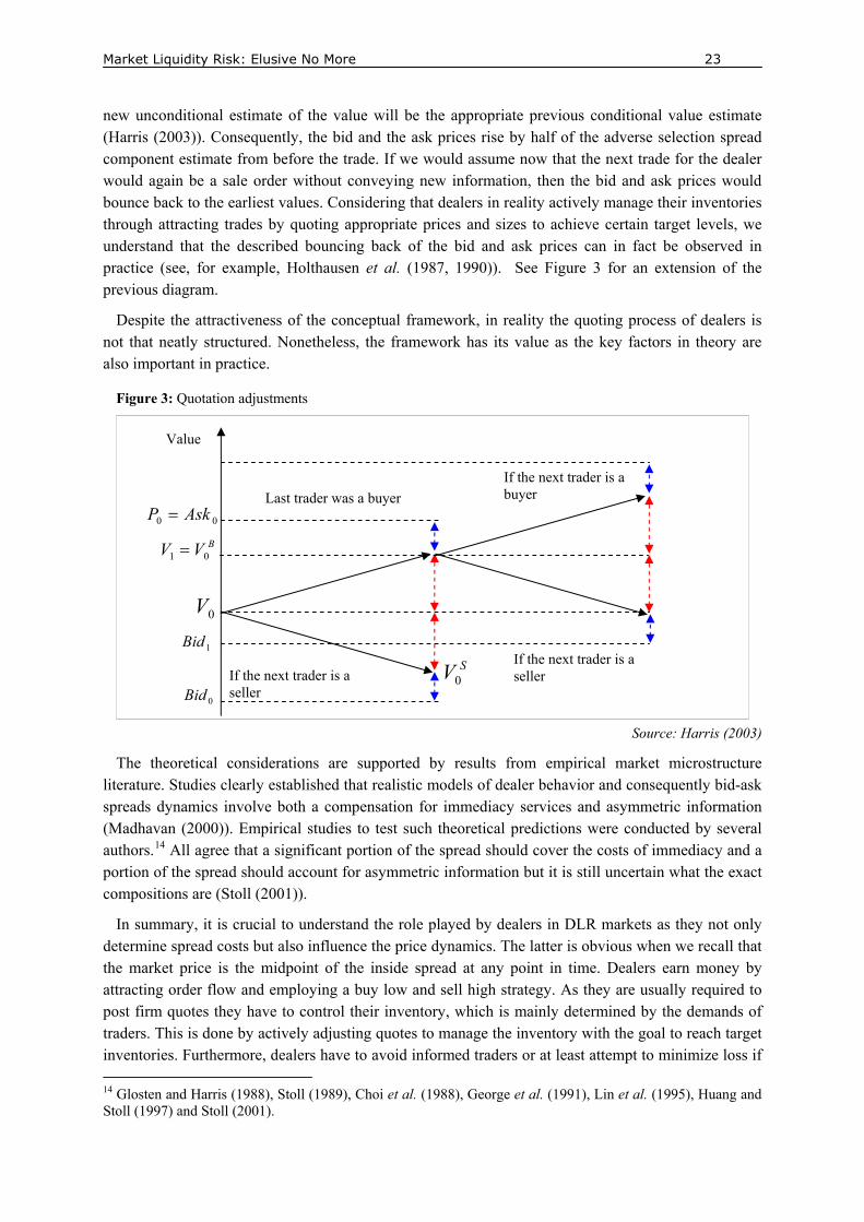
new unconditional estimate of the value will be the appropriate previous conditional value estimate (Harris (2003)). Consequently, the bid and the ask prices rise by half of the adverse selection spread component estimate from before the trade. If we would assume now that the next trade for the dealer would again be a sale order without conveying new information, then the bid and ask prices would bounce back to the earliest values. Considering that dealers in reality actively manage their inventories through attracting trades by quoting appropriate prices and sizes to achieve certain target levels, we understand that the described bouncing back of the bid and ask prices can in fact be observed in practice (see, for example, Holthausen et al. (1987, 1990)). See Figure 3 for an extension of the previous diagram.

Despite the attractiveness of the conceptual framework, in reality the quoting process of dealers is not that neatly structured. Nonetheless, the framework has its value as the key factors in theory are also important in practice.

Figure 3: Quotation adjustments


The theoretical considerations are supported by results from empirical market microstructure literature. Studies clearly established that realistic models of dealer behavior and consequently bid-ask spreads dynamics involve both a compensation for immediacy services and asymmetric information (Madhavan (2000)). Empirical studies to test such theoretical predictions were conducted by several authors.14 All agree that a significant portion of the spread should cover the costs of immediacy and a portion of the spread should account for asymmetric information but it is still uncertain what the exact compositions are (Stoll (2001)).

In summary, it is crucial to understand the role played by dealers in DLR markets as they not only determine spread costs but also influence the price dynamics. The latter is obvious when we recall that the market price is the midpoint of the inside spread at any point in time. Dealers earn money by attracting order flow and employing a buy low and sell high strategy. As they are usually required to post firm quotes they have to control their inventory, which is mainly determined by the demands of traders. This is done by actively adjusting quotes to manage the inventory with the goal to reach target inventories. Furthermore, dealers have to avoid informed traders or at least attempt to minimize loss if 14 Glosten and Harris (1988), Stoll (1989), Choi et al. (1988), George et al. (1991), Lin et al. (1995), Huang and Stoll (1997) and Stoll (2001).

00 AskP =

BVV 01 =

1Bid

If the next trader is a buyer

SV0 0Bid

0V

Value

Last trader was a buyer




they suspect having dealt with one. For our further discussion it is important to note that the demands of traders are the most crucial determinant of quoted prices but not the sole as dealers have to actively manage the risks associated with providing immediacy. For orders that do not exceed quoted sizes the quoted bid or ask price represents the “worst” price at any given moment. We say “worst” as it is possible for traders to realize transaction prices within the spread (i.e., better prices than the bid or ask price).

In our discussion of the behavior of dealers we should not forget that most exchanges oblige their registered dealers to adhere to certain rules that influence their activities. We have seen that dealers face two types of obligations, namely affirmative obligations (provision of continuous quotes) and negative obligations (restriction of own trading). Generally that means that in order to maintain a “fair and orderly market” registered dealers are obliged to deal for their own account when lack of price continuity, lack of depth or disparity between supply and demand exists or when it is reasonable to be anticipated (NYSE Rules). Violations of these rules usually result in fines. These types of rules clearly restrict the spread posting behavior of dealers. The important point to remember is that registered dealers are usually not completely free in their choice of spreads.

Limit-order-book

In pure LOB markets there are no dealers facilitating the functioning of the market. In other words, there is nobody in between the buyers and the sellers, no intermediaries. Orders are matched by a software algorithm that incorporates the rules of precedence of the specific exchange. Because there are no dealers, there is no inventory risk involved. Thus, most market microstructure studies involving spread components do not apply for LOB markets.

Nonetheless, there are naturally bid and ask prices in LOB markets as well. The ask prices in LOB markets are established by previously placed sell limit orders of investors and the bid prices are established by previously placed buy limit orders. Incoming orders are either matched immediately or placed in the limit-order-book and matched according to the precedence rules or expire because of their validity constraints. In LOB markets the midpoint quote (market price) can only change as a result of a trade, the appearance of new limit orders, or the cancellation of some limit orders (Bouchand et al. (2006)). Thus, the supply and demand of traders determines spreads and prices in LOB markets.

Although LOB markets are becoming increasingly important we emphasize dealer markets in subsequent sections as they are still more significant. However, all results generally apply to LOB markets as well, except of course the considerations regarding dealer behavior.

3.8.2 Price risk

As discussed earlier, trading introduces the possibility that the price moves in an unfavorable direction during the time interval between the processing of the order and the execution of the order. The decision for engaging in a trade is among other things a function of the last midpoint quote for an asset. That means that traders commonly would like (expect) to trade at the last quoted price or better but not worse. If, for whatever reason, between the time of the processing of the order and its execution the price moves against the trader’s position beyond what was expected, we can consider the adverse price movement beyond the expected transaction price (i.e., the difference between actual transaction price and the expected transaction price) as a loss/cost. A dealer faces essentially the very same problem. As soon as he has to take a position (inventory), he hopes that an investor will assume a counter position in a short period of time. During the time of him taking the position and the arrival


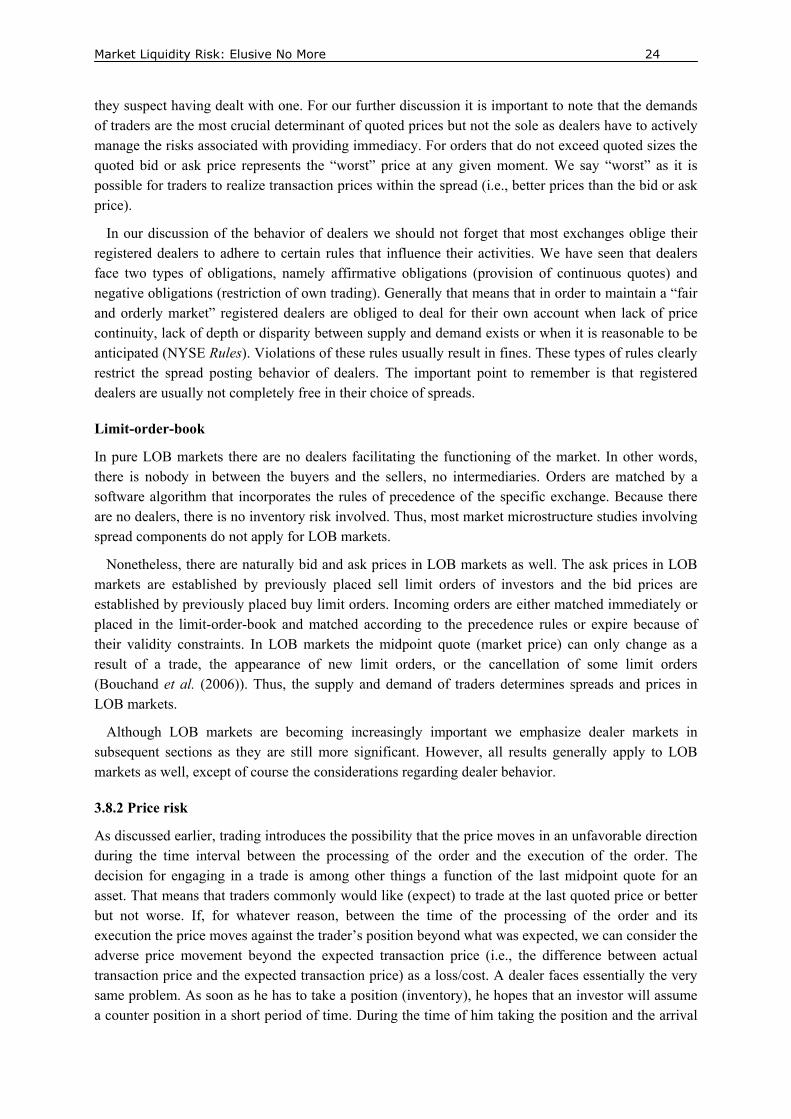
of another investor the dealer is also exposed to adverse price movements. See Figure 4 for a schematic illustration.

Figure 4: Delay in trading

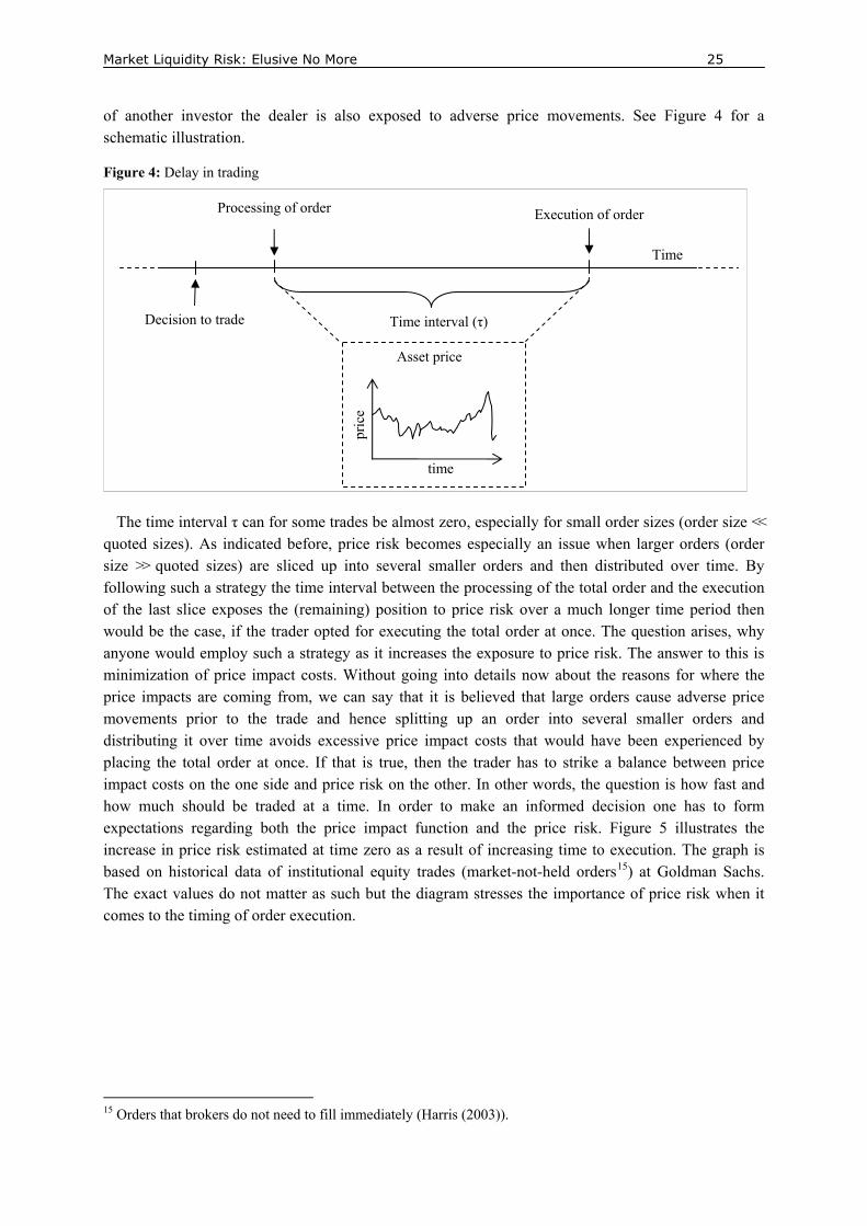
The time interval τ can for some trades be almost zero, especially for small order sizes (order size << quoted sizes). As indicated before, price risk becomes especially an issue when larger orders (order size >> quoted sizes) are sliced up into several smaller orders and then distributed over time. By following such a strategy the time interval between the processing of the total order and the execution of the last slice exposes the (remaining) position to price risk over a much longer time period then would be the case, if the trader opted for executing the total order at once. The question arises, why anyone would employ such a strategy as it increases the exposure to price risk. The answer to this is minimization of price impact costs. Without going into details now about the reasons for where the price impacts are coming from, we can say that it is believed that large orders cause adverse price movements prior to the trade and hence splitting up an order into several smaller orders and distributing it over time avoids excessive price impact costs that would have been experienced by placing the total order at once. If that is true, then the trader has to strike a balance between price impact costs on the one side and price risk on the other. In other words, the question is how fast and how much should be traded at a time. In order to make an informed decision one has to form expectations regarding both the price impact function and the price risk. Figure 5 illustrates the increase in price risk estimated at time zero as a result of increasing time to execution. The graph is based on historical data of institutional equity trades (market-not-held orders15) at Goldman Sachs. The exact values do not matter as such but the diagram stresses the importance of price risk when it comes to the timing of order execution.

15 Orders that brokers do not need to fill immediately (Harris (2003)).

Time interval (τ)

time

pric

e Asset price

Decision to trade

Processing of order Execution of order

Time


Figure 5: Intra-day price risk

-600

-400

-200

0

200

400

600

800

0 to 10s 30 to 1min 5 to 15min 30min to 1hour 2hour to 4hour

Time to execution

Bas

is p

oint

s

Mean-2STD+2STD

Source: Sofianos (2004)

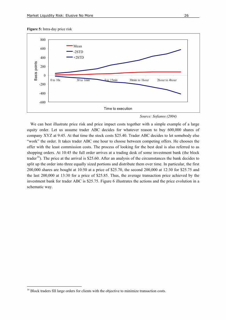
We can best illustrate price risk and price impact costs together with a simple example of a large equity order. Let us assume trader ABC decides for whatever reason to buy 600,000 shares of company XYZ at 9:45. At that time the stock costs $25.40. Trader ABC decides to let somebody else “work” the order. It takes trader ABC one hour to choose between competing offers. He chooses the offer with the least commission costs. The process of looking for the best deal is also referred to as shopping orders. At 10:45 the full order arrives at a trading desk of some investment bank (the block trader16). The price at the arrival is $25.60. After an analysis of the circumstances the bank decides to split up the order into three equally sized portions and distribute them over time. In particular, the first 200,000 shares are bought at 10:50 at a price of $25.70, the second 200,000 at 12:30 for $25.75 and the last 200,000 at 13:30 for a price of $25.85. Thus, the average transaction price achieved by the investment bank for trader ABC is $25.75. Figure 6 illustrates the actions and the price evolution in a schematic way.

16 Block traders fill large orders for clients with the objective to minimize transaction costs.


Figure 6: Price risk and price impacts


The example illustrates the importance of both price risk and price impact costs. The price risk is illustrated by the yellow line, whereas the orange line depicts the price impact of the three orders executed by the investment bank. The yellow line in this case is linearly increasing with time and thus is working against trader ABC’s buy order. The yellow line represents the base price movement of the stock. When we would assume that there are no price impacts, meaning the three orders do not cause any adverse price movement, then we would find the transaction prices at the corresponding times on the yellow line. In that case the best choice would have been to execute the whole order (600,000) immediately at 10:45. Obviously trader ABC could have done that without the help of the investment bank. He would have had filed a market order for 600,000 shares and saved the commission fees. In the presence of price impact it is only possible to execute a buy order at a higher price (a sell order at a lower price) than the yellow line suggests. From the diagram we observe that the orange line actually starts before the first order is executed by the bank. That reflects information leakage. Front runners actually got information about the upcoming orders in some way and acted upon it.

Now if we would assume that there is no base price movement, i.e., the yellow line is horizontal, then obviously the execution prices would have been lower despite the price impact costs. Thus, we can summarize that price risk, the adverse base movement of the asset prices, is a very important factor contributing to the transaction costs.

Although the example illustrates the basic concepts, it is still very stylized as it provides only a glimpse on the problem regarding the price risk involved. It does not provide insights where actually the potentially adverse base price movements stem from. Questions arise such as how can the base price movement be separated from the price impact? Where are the base price movements coming from? What are the driving factors? Where does the price impact come from? What is the relation between the price impact and the base price movement? What role does the dealer play in this? The dynamics of price changes seem to be indeed invaluable for the understanding of transaction costs. We attempt to clarify these issues in the following paragraphs after we briefly discuss opportunity costs.

9:45 Trader ABC decides to buy

600,000 shares of company XYZ

10:45 order arrives at investment bank

$25.40

$25.60

$25.80

13:10 execution completed

$25.70

10:50 first execution

$25.75

12:30 second execution

$25.75 average execution price

$25.85

Trader ABC “shops” order

Investment bank splits order in three 200,000-

share executions $25.35 Base price move

Price move cause by price impact


3.8.3 Opportunity costs

Opportunity costs are not known before the trade. The easiest way to quantify them is to incorporate the time value concept into some formalized model that would capture the uncertainty of the other transaction costs such as bid-ask spread, price risk and price impact. Another approach is taken by Perold (1988). In his popular implementation shortfall measure he describes the opportunity costs as the amount by which the benchmark has changed in value during the course of the transition, weighted by the share of the total order that has not been invested in the target stock/portfolio. More formally we can write the opportunity costs of the sale of a portfolio as,

( )( )1

Ne e b

i i i ii

n m p p=

− −∑ , (3.1)

where

in = number of shares of security i held in benchmark

eim = number of shares of security i held at the end of the

execution of the total order

eip = price of security i at the end of the transition

bip = price of security i at the beginning of the transition

According to this specification the opportunity costs include indirectly price risk and any potential price impacts of the own trading. In our opinion the metric provides a misleading picture of the opportunity costs as the benchmark is a hypothetical costless and instantaneous transition at the beginning. In other words, it measures the opportunity costs against a transaction at the midpoint quote (no price impact) at the beginning of the transition. This seems rather odd as such a transition does not exist. Thus, in many cases the opportunity costs calculated like this overestimates the forgone opportunities because of impact price costs. In addition, Perold’s metric is intended to be an ex-post performance measurement for the transition17 of a portfolio. The problem with opportunity costs arises when one wishes to disentangle the price impact and the base price movement empirically from real data. In theory this is easier as one assumes a price evolution of the base price movement (e.g., geometric Brownian motion) and determines separately the price impact say from a regression analysis. This way, one could estimate the opportunity costs before the trade. However, in our opinion if opportunity costs are to be taken into consideration at all, it would be more reasonable to only discount at an appropriate rate.

3.8.4 Price impact costs

Let a trader face the following situation: he holds a certain amount q of an asset, which he would like to sell at the prevailing market price p. As we have seen this is per se not possible, as the market price is actually the midpoint quote (i.e., midpoint of the inside spread). Thus, he can only expect to sell at the prevailing bid price if the desired transaction size does not exceed the quote size (and if the quoted bid price and size are actually firm quotes). When the desired transaction size q is actually larger than the quoted size (i.e., quote/market depth) and the trader decides to file the order anyhow, then the

17 In practice the process of arriving from a given position to a desired position is sometimes called transition. Thus commonly companies offering to help perform this process call themselves transition managers. This is similar to block traders.


order will not be liquidated fully at the prior quoted bid price. Instead he will have to sell q at an even lower price than the bid price because either the corresponding dealer wants a discount based on inventory management considerations ( and/or asymmetric information) or because the next best offer from a counterparty to buy the asset is offered at a lower price (the latter will occur in limit order books). Thus, the trader experiences an adverse deviation of the transaction price from the market price or better the bid-price. The example is symmetric for a desired buy order with the only difference that in case of a sell order costs occur as a loss on the investment whereas in case of a buy order they occur as an extra charge. The problem is illustrated in Figure 7.

Figure 7: Effect of position size

Source: Bangia et al. (1999)

In the described example the adverse deviation of the transaction price from the market price or the bid-price are the price impact costs. One can clearly see that the determination of the price impacts depends on the choice of the benchmark price against which the actual transaction price is compared. Principally in literature we can distinguish between two types of price impacts, (1) post-trade price impact and (2) pre-trade price impact. Pre-trade price impacts are described in the prior example and refer to the adverse deviation of the actual transaction price from a benchmark price. However, it could very well be that the actual transaction price is at the bid or ask price or even within the spread but results in a price impact after the actual trade. This we call a post-trade price impact. But we have to be very careful here as we have to define what prices we are talking about. We should not mix up midpoint prices (or equivalently market prices) and actual transaction prices. In the end only actual transaction prices matter but midpoint quotes still have a very important signaling function to most market participants. For traders, actual transaction price and pre-trade price impacts are more important than post-trade price impacts. See Figure 8 and 9 for illustrations.18

18 Recall that the displayed spread in the figures would represent the inside spread. In addition, the reader should take note that although the trade is arrange with a single dealer the order can influence the quotes of the other dealers as well, since they have access to information of all order flow data.

Position size Quote Depth

Asset price

Bid

Ask


Figure 8: Post-trade price impact for a buy order

Figure 9: Pre-trade price impact for a buy order

Let us define the two types of price impact more formally,19

Post-Trade Price impact = 1 0S S− (3.2)

0S = Last midpoint quote of inside spread before the

processing of the order

1S = Earliest midpoint quote of inside spread after the execution of the order

Equivalently, we could use the proportional price change,

Post-Trade Price impact = 1

0

1SS

− (3.3)

The pre-trade price impact is consequently defined as,

Pre-Trade Price impact = 0S S− (3.4)

0S = Last midpoint quote of inside spread before the

processing of the order

19 All subsequent formulations of price impacts are for buy orders. For sell orders we just have to change the sign of the equations e.g., the first equation for the post-trade price impact for a sale order would be 0 1S S− , as we would expect that sell orders lower the prices and buy orders increase prices.

Ask

Midpoint

Bid

Transaction price

Pre-Trade -Price impact

Effective half-spread

Ask

Midpoint

Bid

t0 t1

Transaction price

Post-Trade -Price impact

Effective half-spread


S~ = Transaction price/traded price20

Or the proportional version,

Pre-Trade Price impact = 0

1SS

− (3.5)

In the context of pre-trade price impacts we can introduce the terminology often employed in practice of at-the-spread, in-the-spread and out-of-the-spread. For at-the-spread transactions the traded price is equal to the quoted bid or ask price before the processing of the order. For in-the-spread transactions the traded price is better than the corresponding quoted bid or ask price prior to the trade. Consequently out-of-the-spread transactions involve pre-trade price impacts, as the traded price is worse than the corresponding bid or ask price.

The post-trade price impact is not as such interesting from a practical point of view but could be used in case traded price data are not available as a proxy or to understand the dynamics of the midpoint quote of the inside spread, which could turn out to be very well interesting for practitioners. Thus, for traders wanting to place orders the pre-trade price impact is of crucial importance as it determines the costs relative to their expected transaction prices. But here lies a bit of a problem as one might question why the midpoint quote of the inside spread should be used as a benchmark price and not the bid or ask price just prior to the processing of the order. It is true that it is possible for the order to trade within the inside spread, thus closer to the midpoint quote. In those cases the use of the bid or ask price as the expected transaction price would be an overestimation but generally the use of the them as a benchmark price is certainly more prudent. In fact, we have illustrated this reasoning already in Figure 9, where the pre-trade price impact is the distance from the ask price to the transaction price. Thus, let us restate our definition of the pre-trade price impact as follow,

Pre-Trade Price impact = AS S− (3.6)

AS = In case it is a buy order we use the last ask price quote of the inside spread before the processing of the order21

S~ = Transaction price/traded price

However, we could even go one step further and refine our definition of pre-trade price impacts (post-trade price impacts) to allow even more general benchmark prices V,

Pre-Trade Price impact = S V− (3.7)

V = Benchmark price

Up until now we have implicitly assumed that in case of a pre-trade price impact solely the processing of the individual order induces an adverse movement of the bid or ask price at which we can trade. Thus, we imply a simple one-dimensional cause and effect chain. In literature (see Chan and Lakonishok (1995, 1997) and Patel (2001)) have been attempts made to separate base price movements (price risk) from the price impact by incorporating a correction term. Usually the

20 Throughout the text the terms transaction price and traded price are used interchangeable. 21 In case of a sell order we would use the last bid price quote of the inside spread before the processing of the order in conjunction with a corresponding change in the sign.


correction term is the return on a large market index multiplied by the beta (covariance of the market return and the individual security return). Thus, we would arrive at the following equation,

Pre-Trade Price impact = ( ) ( )Pr eS V M Mβ− − − (3.8)

M~ = Index price at the time of execution of the order

eM Pr = Index price at the time just before the order is

processed

β = Slope coefficient of the regression of excess returns (returns exceeding the risk free rate) of an asset on excess returns of the market (using midpoint quotes of the inside spread)

Conceptually it is desirable to implement a correction for the base price movement (price risk) of the security in order to isolate the price impact of the trade but this introduces several difficulties. The primary question that we should ask is whether it really makes sense to separate price impact and base price movements at all and secondly if it is possible.

Price impact versus base price movement

The first question that arises is whether we can and should separate price impacts from base price movements at all. Let us recall that generally price risk is nothing else then the movement of the price (usually the midpoint quote but not necessarily) through time. Thus, if we would not engage in any trading between say time t0 and t1 we would simply observe at t1 that, say, the midpoint quote changed between that time interval from A to B for whatever reason. The difference between B and A then represents the base price movement of that security between t0 and t1. That is very simple but if we would engage in trading during t0 and t1 and we want to determine the price impact of our trade we face the problem that we have to disentangle the base price movement and the impact of our proposed trade on the transaction price. To approach the problem we have to first determine why the transaction price would deviate from the last quoted ask or bid price before the trade at all. If we can identify the main drivers we might be able to extract the impact of our processed order on that deviation.

What moves prices?

The demands of traders expressed as signed order flow are at the center of price dynamics. The formation of demands at the level of traders depends on various aspects but a key component is the valuation of an asset at a given point in time. Theory would like to let us believe that traders are rational beings and hence draw similar conclusions with regard to asset valuations. However, this is not the case. Opinions deviate from person to person. The key argument for our position is that there are necessarily different interpretations of a given information set. If we think this thought to an end we arrive at an explanation for the price discovery22 process. The explanation is very similar to the one described by Brandt and Kavajecz (2004) for the bond market and Evans (2002) and Evans and Lyons (2002) for the currency market. Let us consider a set of market participants, each of whom has his own opinion or model of how asset prices relate to company specific, market factors and/or economic fundamentals. Some participants might even possess private information. In this incomplete and heterogeneous information structure, market participants trade according to their subjective opinions /

22 Price discovery is roughly the mechanism by which asset prices change.


valuations. Since the time interval between the filing and the clearing of orders is not instantaneous market participants can infer information about the subjective valuations of all other participants from the aggregate order flow. This information may result in revisions of their own subjective valuations. For instance, if the aggregate buy orders at the quoted price exceed the aggregate sell orders, market participants with lower subjective valuations may decide to revise their valuations upward. The amount by which the revision may occur depends on how much they trust their own valuation.

Market microstructure theory supports these considerations of the price discovery process. The main conclusion that can be drawn from literature is that order flow, the sequential arrival of buy and sell intentions of traders, plays an essential role in the price discovery process. According to papers by Glosten and Milgrom (1985) and Kyle (1985) order flow is so important because of the (perceived) presence of information asymmetries, which triggers adverse selection effects. As we have discussed in the section about dealer behavior dealers set their bid and ask prices to reflect the trade-off between losses to trading with informed traders and profits to trading with uninformed traders. Empirically Hasbrouck (1991) shows, with the help of vector autoregression analysis (VAR)23 for stocks, that order flow influences prices as predicted by theory. More specifically, buy order raise prices and sell order lower prices. Similar findings are documented by Evans and Lyons (2002) for the foreign exchange market as well by Brandt and Kavajecz (2004) for the bond market.

Does this mean that asset prices are solely determined by demands of traders? The answer is no, because we would neglect the important role played by the dealers in the price discovery process. 24 Thus, in summary order flow and dealer behavior (in dealer markets) seem to be the major contributors to price changes. As we have seen, active inventory management of dealers is mainly but not exclusively a function of order flow. Order flow is solely the expression of the demands of traders. Let us discuss the drivers of supply and demand of assets in a bit more detail before we go back and describe the influence of our findings to the price impact considerations.

Supply and demand

We have already seen that one key factor that determines the varying demands for assets is the necessary difference in opinions. It has to be understood that the difference in opinions is always determined from the position of the subject. In other words, not only the individual judgment of the value of asset but also the value of the asset for the individual is important. That means that the motivation of the individual of why he is interested in trading that asset has an influence on his valuation (e.g., on-the-run securities for bonds). Individual investors have different opinions at what price and at what time they wish to buy or sell an asset. They have a certain opinion about the value of the asset and a certain motivation. The demands of traders are finally expressed as signed order flow by filing orders. The combination of all buy and sell orders (market order and limit orders) from all traders at a time form the demand and supply curve for an asset at that point in time. Muranaga and Shimizu (2001) distinguish between effective supply and demand and observable or explicit supply and demand. Effective supply and demand reflects the aggregation of the investors needs at a certain time whereas the explicit supply and demand is a reflection of this effective supply and demand in observable order-book profiles and order flows. Possible reasons why the effective supply and demand

23 Vector autoregression (VAR) is a technique that attempts to capture the evolution and interdependencies of a set of n variables over the same time period as a function of their own past evolution. Thus each variable has an equation explaining its evolution based on its own lags and the lags of all the other variables in the model. 24 The answer would be ‘yes’ if we are dealing with a pure LOB markets.


does not necessarily be equal to the explicit demand and supply are costs in the form of commission, fees, taxes and perceived information asymmetries.

Figure 10: Supply and demand curves

The starting point in the very beginning was the definition of frictionless markets. One assumption was that any trader can buy or sell unlimited quantities of the relevant security without changing the security’s price. Thus, without considering price impacts for a moment, that assumption is equivalent to a perfectly elastic supply / demand curve (i.e., horizontal line at the given midpoint quoted price – see Figure 10). However, this is not very realistic as it has been shown in various empirical studies that at least for stocks25 downward sloping demand curves are common (Shleifer (1986), Kaul et al. (2000), Wugler and Zhuravskaya (2002) and Greenwood (2004)).

Price formation process – a framework

It might be useful to bundle the discussed aspects regarding the trading environment together and create a unifying framework for the price formation process (i.e., price discovery). The framework has the intention to provide an intuitive explanation of the price formation process and the resulting consequences, namely transaction costs. Furthermore, the framework is based on the simple, yet powerful, idea that the price formation process must be the result of the collective behavior of humans (i.e., traders) subject to certain constraints. Thus, in that sense, financial markets are not black boxes per se but understandable phenomena. However, the mechanisms and pathways seem to be too complex to be grasped. This can lead to the false conclusion that we are dealing with phenomena governed by unknown laws, where we can only hope to discover patterns in the outputs.

The framework is illustrated in Figure 11. We see that for understanding the price formation process we need to understand two main stages. The first stage is the formation of supply and demand of traders and the second is the price quoting process. We see that the demand and supply on the level of the traders is formed because of two factors, namely, the difference in opinions and the motivation of trading. We can go one level deeper and identify three factors that help to explain the difference of opinions: (1) information, (2) model and (3) experience. Evidently, differences in the level of

25 We do not see a good reason why we would not expect that for other assets as well.

(a) Perfectly elastic

demand pr

ice

size

(b) Inelastic demand

(downward sloping)

pric

e

size

(c) Perfectly elastic

supply

pric

e

size

(d) Inelastic supply

(upward sloping)

pric

e

size


information or the perception of it can be responsible for different opinions. The presence of public information alone does not mean that everyone is aware of them. Further, it is important to stress that all information signals are in the end interpreted by individuals. Thus, the information content of a specific signal necessarily differs from investor to investor. However, there can also be a “real” difference in information signals in case there is private information present. The second factor is the usage (or not) of different models. This is usually not applicable to the average private investor as he does not use any formalized models, but for most institutional traders it does play a crucial role.

Figure 11: Price formation process

ExperienceInformation ConstraintsAdvancedtechniques

Traders

Difference inopinions

Motivation oftrading

Model Time horizon

Supply Demand

Order flow

Rules ofprecedence

Regulations

Inventory

Constraints

Competition

Information

Regulations

Market price

LOB DLR

Bid Ask

Commonly some sort of formalized model is used to complement the “natural” assessment process of information content. Now we actually touch on the last factor, experience. Experience is the key factor in every human action. Every information and decision in all situation of life are formed in validation with the own personal experience established throughout our entire life (Roth (1996, 2003)). Thus, if not a formalized model is doing the entire work (even then it was created by humans) there is a human forming an opinion of some given information signals and that means that actually the personal experience of this human has the last word in it. The cross validation with the personal experience is an unconscious process and is thus not directly perceived.

The second branch in our framework that affects the supply and demand is the actual motivation of trading by investors. It is clear that not all investors have the same motivation in trading. We have seen in the beginning that the buy side in financial markets consists of a highly diverse group of players, each with different trading motivations.26 Here we point out that there are three main factors

26 The reader should take note that in fact the enormous complexity of different trading motivations in today’s financial markets makes any potential modeling efforts of the supply and demand dynamics seem futile. See


characterizing the trading motivation: (1) time horizon, (2) advanced techniques and (3) constraints. The desired time horizon of the investor influences the dynamics of his demand for an asset or his willingness to sell it at a given point in time. Under advanced techniques we summarize all sophisticated reasons for buying, holding or selling an asset. Those include among others, hedging, various hedge funds strategies (e.g., market neutral strategies) and diversification. The distinction is made here because the motivations of those can lead to quite different demands at certain times compared to other more conventional motivations. The last aspect is self-explaining as every trader is constrained in some way, be it by regulatory constraints, capital constraints, loss limits, funding withdrawals or debt servicing. These influence the willingness to buy or sell at a given price. Although the identified driving factors for the motivations and the differences in opinion are very important, we are aware they are certainly not exhaustive. For example, a trader’s mood on a given day might very well influence his trading decision.

It should be clear that a certain finite number of investors form the supply and demand curves for a specific asset. This implies that every individual asset has its own demand and supply curves. In addition, it should be apparent that the demand and supply curves are dynamic as it is not reasonable to assume that the factors described in the framework are constant. In addition, they are stochastic as they do not move deterministically through time. Hence, if we would like to understand the price movements of an asset we would have to know the stochastic supply / demand curve of it. The most important factors in our opinion governing the stochastic supply and demand curves of assets were identified above. The difficulty would be to quantify and model them.

The second stage in our framework is the price quoting process. We have to distinguish between dealer dominated markets and pure limit order markets. For the DLR market Figure 11 indicates that the dealer has to face six major factors: (1) order flow, (2) exogenous information shocks, (3) inventory pressure, (4) constraints, (5) competition and (6) regulations. All six factors have to be taken into account by dealers in their job to provide immediacy to investors. The most important factor is the uncertainty surrounding the future order flow of other market participants. Dealers need to anticipate future order flow at any given time during the day and accordingly quote bid and ask prices to allow them to earn a positive margin. Certainly exogenous information shocks have to be considered by dealers as well in order to prevent stale quotes and losses. Exogenous information shocks can lead to instantaneous revaluations of quoted prices by dealers without first going through the signaling function of signed order flow. Besides, dealers have to consider capital constraints as well as the actions of their competitors. Finally, dealers are usually strictly regulated because of their important role in making financial markets work. Regulations usually include provisions of continuous quotes, restriction of own trading, price smoothing and minimum tick sizes. Another aspect that we have discussed is that dealers actively manage their inventory. This means that they set quotes to attract certain kind of order flow in order to reach their individual target inventory levels.

In our discussion earlier and in this framework as well, we distinguish between dealer dominated markets and pure limit order markets. Since in pure limit-order book markets dealers are completely absent the price quoting process depends solely on the order flow governed by a given set of precedence rules and other regulations.

Harris (2003) for an illustrative and very detailed taxonomy of different traders. On the other hand, it would seem that this complexity is what makes financial markets “work” rather smoothly most of the time. We will see in the discussion of financial crises in later sections that a lack of it could distort the smooth working of markets.


Price impact dynamics

Our brief digression regarding the drivers of price changes was motivated by establishing whether it makes sense to separate price impact costs from base price movements. Although we have identified that order flow is the primary driver we would have a hard time to distinguish the impact of our order flow from the impact of other’s order flow, let alone considering the influence of the other factors in Figure 11. This seems an impossible task and we shall not attempt it. Thus, it becomes obvious that using a correction term as proposed in earlier sections involving the correlated movement of a market index is a very crude method at best. Using this method implies the assumption that the factors for the market index (or better for all the securities compromising the index) are identical to the ones for the individual asset. There is no good reason to accept this assumption on any ground in our opinion. Thus, we conclude that we cannot practically correct the price impact measure for base price movements.27 However, what can be done is to analyze the dynamics or patterns of price impacts. Identifying not only the size but also patterns of price impacts can be very valuable for modeling purposes as we shall discuss in later sections.

It is important to stress that there is not a single factor determining the magnitude and/or dynamics of the price impact but several. That means that the interpretation where solely the filed order induces a price movement before the order can be executed is too restrictive. In other words, there are other factors that can result in an adverse price movement that are independent of the filed order. 28 Hence, it is reasonable to distinguish between exogenous factors that are independent of the individual orders even if substantially large, and endogenous factors, that are specific to one’s order. This distinction loosely follows Bangia et al. (1999) considerations. See Figure 12 for an illustration of the distinction.

Figure 12: Determinants of price impact

Other factorsAggregateorder flow TimingSigned order

size

Price Impact

Exogenousfactors

Endogenousfactors

Identity

The exogenous factor reflects the order flow of other investors, which is primarily determined by their motivation to trade and the difference in opinion stemming from the subjective interpretations of information signals regarding the value of the asset. As we have seen, aggregate order flow is a crucial factor for the price setting behavior of dealers and thus will have an influence on the price impact received by individual traders. We have several other factors that are independent from the individual order, such as for example the current dealer’s inventory level or his target level. The endogenous part reflects the influence of the characteristics of the individual order. The most important information content of the order is the order size and possibly the identity of the trader. As we have discussed, the sign and the size of orders might make other market participants, including the dealers, reevaluate

27 This conclusion does not say that the separation of price impacts and exogenous price movements is useless in principle, only that the method illustrated in equation 3.8 is questionable. In fact we will see in later sections that in theoretical models it is possible and desirable to make a distinction between the two concepts. 28 For the mentioned reason price concession would actually be a more sensible and correct term for the concept but because of its widespread use we shall continue to use the term price impact.


their subjective valuation and hence their desire to engage in transactions themselves. 29 The order size is always visible to dealers and at least in stock markets also to other market participants. The identity of the trader in organized markets is generally not known by other market participants. However, for example, in stock markets there exist upstairs markets30, where identities are communicated with the hope to reduce possible price impact. In addition to organized markets there exist OTC markets in which identities are commonly known by counterparties. In case identities are not known, traders and dealers might attempt to guess the identities of the traders behind certain trades in order to gauge the information content of the trades. This will influence the aggregate order flow and hence the magnitude and the dynamics of the price impact. The sign and the size of an order will also govern the consequences for the inventory of the dealer and hence the size and the dynamics of the price impact. Furthermore, in trading the timing is also important and might influence the level of the price impacts.

From theoretical considerations we might expect different dynamics regarding the price impact depending on the dominance of the prevalent factors driving the price impact. In fact a large body of literature suggests that at least for stocks price impacts consist of two components, a temporary and a permanent price impact (see as an early reference Holthausen et al. (1987, 1990)). As the names imply, a part of the initial price impact (i.e., price change) is transitory in nature and dissipates in a short period of time, whereas another part of it remains even after that time and is deemed permanent.

Figure 13: Price impact functions

Source: Hisata and Yamai (2000)

Market microstructure explains the existence of the temporary (transient) price impacts mainly by inventory control effects. However, price discreteness, price pressure, order fragmentation and obliged price smoothing also play a role. The permanent price impact is argued to exist because of asymmetric

29 The attentive reader might recognize the strong link to Bayesian statistics theory, where in the wake of new information the prior subjective probability assessment is reevaluated. In fact, extracting information from order flow is similar to Bayesian learning and is discussed in several market microstructure papers focusing on the effect of asymmetric information rather then inventory management. 30 The upstairs market refers to transactions that are not sent to the exchange floor for execution but are completed through a network of trading desks of major brokerage firms and institutional investors that communicate with each other by means of electronic systems and telephones to receive more favorable prices than on the exchange floor primarily by attempting to convince others that the desired block sale does not convey information but is motivated by utilitarian aspects.

Permanent portion

Temporary portion

PosttTratetPr

Time

Asset price

PostP

TraP

ePPr

Post-transaction price ePPr : :TraP :PostPPre-transaction price Transaction -price


information, i.e., the order incorporates private information about the asset. The concepts of temporary and permanent price impacts are best illustrated in Figure 13 for a seller-initiated order.

The distinction between temporary and permanent is to some extent arbitrary but nonetheless it is important to consider that there is evidence for a bouncing back from the effective transaction price to not quite to the original level of the bid/ask price (or midpoint quote) before the transaction. This has be documented for stocks by Holthausen et al. (1987, 1990), Biais et al. (1995), Degryse et al. (2004) and Coppejans et al. (2003). Evans and Lyons (2002) find similar results for the foreign exchange market. Hasbrouck (2004) and Kempf and Korn (1999) show comparable results for the futures market. For the bond market Cohen and Shin (2003), Green (2004), Brandt and Kavajecz (2004), Edwards et al. (2005), Cheung et al. (2005) and Lawrence and Piwowar (2006) show the existence of similar price impacts dynamics. For a more detailed discussion of the similarities and differences of the asset markets in terms of price impacts see later sections.

Let us now discuss what aspects price impact functions should incorporate according to our findings. First, in all dealer markets we would in principle expect the existence of temporary and permanent price impacts. Thus, we would need two separate functions if we are interested in the dynamics of the impacts. One could argue that traders are only interested in the initial price impact since it determines the immediate loss. In our earlier terminology that translates to the pre-trade price impact. In case the trader does not split a large order into smaller parts he would indeed only care for the pre-trade price impact or the temporary price impact. But as soon as he would split an order up to minimize price impacts, he would need to take into consideration the permanent impact or post-trade price impact as well. Another interesting evidence from empirical studies is that there is an asymmetry between buyer-initiated and seller-initiated orders when it comes to the magnitude of price impacts. Buyer-initiated orders induce larger impacts than seller-initiated orders (Holthausen et al. (1987, 1990), Chan and Lakonishok (1993, 1995)). Thus, modeling the price impact dynamics would require now in total four different equations, two impact functions for boch, purchases and sales. Furthermore, Hasbrouck (1991) identifies three points that should be taken into consideration when attempting to model price impact dynamics. First of all, it was demonstrated that at least for stocks there exist serial dependencies in trade signs because of inventory control (dealer), price pressure and order fragmentation (splitting up of larger orders into smaller parts) (see also Bouchaud et al. (2006)). A second point is that is it very likely that the “information” impact is distributed over time because of lagged adjustments and exchange-mandated price smoothing. This can be important for estimation equations where lagged values have to be implemented. As a last point, Hasbrouck suggests that only the trade innovation, which is the unexpected trade size, considering the other effects such as the mentioned serial dependencies, should be used for explanatory purposes.

Up until now we did not go into detail on what the price impact should be a function of. Earlier we said that it should be a function of trade size. In fact most cited studies followed this approach. However, this can only be approximately right, as there are exogenously factors that influence the aggregate order flow and hence the inventory management of the dealers. Nonetheless, in order to capture the individual characteristics of the order, the transaction size is surely the best choice. Empirical findings suggest that at least for equity markets the pre-trade price impact and the post-trade price impact are both non-decreasing in trade size. In other words, the more you want to trade in excess of the quoted sizes, the stronger will be the adverse deviation from the benchmark. There are two explanations for the dynamics. First of all, large transactions are more problematic for the inventory management of dealers, i.e., large orders usually push actual inventory levels far away from target levels. A second reason is that large orders might carry more private information than smaller


orders, as traders must have a good reason for unloading such a large amount of assets on this precise moment. Although large order do not necessarily imply the presence of asymmetric information, it is not unreasonable for other traders as well as dealers to believe so.

3.8.5 Magnitude of transaction costs

Several empirical studies have attempted to analyze the magnitude of transaction costs. Results directly depend on the specific definitions employed. If we look at the country level we can refer to the work of Domowitz et al. (2001). They analyzed transaction costs of institutional equity trades in 42 countries and provide figures that can be used to judge the importance of transaction costs in a wider context. The average of the total transaction costs, consisting of explicit and implicit costs, 31 across 42 countries is 71.3 basis point of the order value. The explicit costs account for 46 basis points (2/3) and the implicit costs for 25.3 (1/3) basis points. It is clear that the estimates for the implicit transaction costs depend on the choice of the benchmark price and should be taken with caution. Nonetheless, they provide some ballpark measures. Maybe a more specific example is provided in Bikker et al. (2006) where the market impact of the equity trades of the largest Dutch pension fund is analyzed. They find that the average market impact costs equal 20 basis points for buys and 30 basis points for sells. Again we do not agree with the methodology chosen as they employ a correction factor for base price movements similar to one discussed earlier, still it gives an impression on transaction costs for stocks. A final example for the magnitude of stock market price impacts is given in Figure 14. Here the price impacts are categorized by order size relative to daily volume and by market capitalization. Clear estimates for other asset markets are lacking but some evidence suggest that transaction costs in equity markets are the larger than in other markets.

Figure 14: Price impact costs for equities

11

28 2733 37

47 5060

77 82 85

37

56 58 5771

90

112

128

159 162168

0

20

40

60

80

100

120

140

160

180

< .25% .25 - .5% .5 - .75% .75 - 1% 1 - 2% 2 - 3% 3 - 5% 5 - 10% 10 - 15% 15 - 25% >25%

Order size relative to daily volume

Bas

is p

oint

Large cap

Small cap


31 Domowitz et al. (2000) distinguish between explicit costs, which are the direct costs of trading such as broker commission costs, taxes, fees etc., and implicit costs, which are price impact costs. They define the price impact costs as the percentage difference between the transaction price and the mean of the day’s open, close, high and low prices.


3.8.6 Minimizing transaction costs

From our discussion of transaction costs it seems that traders can influence the magnitude of the incurred transaction costs to a large extent. Decisions made by traders can have an influence on both the certain (fees, commissions and taxes) and the uncertain (spread, price risk, opportunity costs and price impact) transaction costs as we have distinguished them. However, the certain transaction costs are less likely to be influenced by the trader’s decisions to a large extent although commission fees might be reduced or eliminated by choosing optimal order routing. More interesting are the uncertain transaction costs and the influence traders can have on them. The first cost component, the half spread cannot be significantly influenced directly, although the choice of a good broker may enable traders to receive more favorable bid or ask prices at least for orders smaller than the quoted sizes, because of the broker’s market power as a provider of order flow. Similarly, price risk and opportunity costs can be seen as exogenous from the individual trader’s perspective. To be more precise, the dynamics of the price base movement are exogenous and not the duration of the exposure. Traders can very well determine to a certain degree how long they are exposed to price risk in case larger orders are split up into smaller orders and distributed over time. Still, this is only a rough assumption at best, as we have seen that individual order flow can make other traders change their opinion about asset values. Consequently, individual order flow can influence aggregate order flow as well. As a result, the formerly exogenous price risk has to be deemed partially endogenous and hence assuming price risk being exogenous during the execution time of the order is not completely correct, but not a strong assumption either.32 The last cost component that is uncertain before a trade are the price impact costs, both pre-trade price impacts and post-trade price impacts. As we have discussed earlier, the main determinant of the magnitude of price impact costs is the trade quantity. Price impact functions that are non-decreasing in trade size, as it is the case for most financial assets, give rise to an optimization problem for each trader who wants to execute an order that is larger than the given market depth. To see this, we have to understand the balancing act between price impact costs and the exposure to price risk.

One possibility to avoid high pre-trade price impact costs is to split a large order into several smaller ones and distribute them over time. As a result, we will be able to reduce the pre-trade price impact costs by selling closer to or at the bid/ask price. Theoretically one could divide any order into infinitely small parts and avoid almost all pre-trade price impact costs. Of course this is not possible in practice, but splitting orders smaller or equal to the quoted sizes to avoid price impacts is possible. However, by distributing the smaller orders over time we introduce price risk. In other words, between the first execution of a part of the total order and the completion of the last order part the price of the asset can move against us. Of course, it is also possible that the price is actually moving in favor of our uncompleted orders, that is the bid price increases or the ask price decreases but the risk of adverse movements is there. Thus, a trader wishing to file a large order faces the dilemma of either accepting a large pre-trade price impact and file the whole order immediately or expose his position to price risk by splitting up orders but reducing price impacts. This problem was exemplified earlier in Figure 6 for a large equity order.

This problem could mathematically be reduced to an optimization problem if we can formulize the pre-trade price impact and the post-trade price impacts (or equivalently the temporary price impact and the permanent price impact) dynamics and the price risk. The base price movement is not such a problem in principle as it could be formulized by say a geometric Brownian motion. More problematic 32 The assumption probably gets weaker the longer it takes for an order to be executed because more market participants might be able to observe the presence of the individual order flow.


are the price impact functions. We are not going to formally state the optimization problem here and consider its implication, as that will be done in later sections, but we shall discuss the basic requirements for the price impact dynamics.

3.8.7 Requirements for the optimization problem

We have already discussed the requirement that the price impacts functions must be non-decreasing in quantity size (at least for equity). Furthermore, research suggests on basis of theoretical and empirical considerations that impact functions are rather concave or linear than convex. From what we have learned, price impact functions should be stochastic, i.e., are random and change over time. The demands by traders and dealers, which mainly characterize the price impact functions, are not constant over time and not known. The best solution is to let the price impact functions be stochastic in the first place. One could get around the problem by estimating some coefficients from historical data and assume the function is fixed for some short period of time and then re-estimate the coefficients periodically. Another important aspect is that it is very likely that every asset in an asset class has its own price impact functions. Clearly in case a trader manages a portfolio the effort of estimating and optimizing the trading strategy for every individual asset appears to be formidable. In that case it could very well be possible to group assets in certain categories according to homogenous characteristics. The underlying logic for grouping certain assets into classes must be to capture assets with common factors characterizing the order flow patterns as described in Figure 11.

Beside the price impact functions one must also incorporate the half spread into the optimization problem in some way, either as separate factor or indirect in a discount factor that encompasses the effective half spread. Similar to the price impacts, the spread factor should also be considered to be stochastic. Factors that are not directly related to the transaction costs by itself but should nonetheless be taken into account are internal crossings, hedging against base price movement with future contracts and other practical considerations.

3.9 Other asset markets

Here we shall discuss the main differences between the most important asset markets in terms of market structure and transaction costs. We analyze the characteristics of the bond market, the currency market, the option market, futures market and more generally bilateral negotiations in OTC markets.

3.9.1 Fixed income market

Generally, one distinguishes in the fixed income market between primary and secondary markets. In the primary markets fixed income securities are issued commonly in the form of auctions. These securities are subsequently traded in the secondary market. The fixed income market structure can be divided into three groups: (1) issuers of fixed income securities, (2) financial intermediaries and (3) investors.

The group of issuers mainly consists of governments, municipalities and their agencies, corporations and commercial banks. The main objective for the issuers is to place the securities without any problems in the primary market and obtain reasonable prices for them. Financial intermediaries are for the most parts banks (investment and commercial) and inter-dealer brokers. Principally intermediaries offer various services to issuers and investors for fees. Services for issuers consist of assistance in the marketing, pricing and distribution of securities.


For our discussion more important is the fact that the financial intermediaries are the dealers in the secondary market. The tasks, objectives and risks are the same for them as we have discussed in earlier sections. However, unlike stocks, bonds are predominantly traded through OTC markets where the major players are banks. Although bonds are also traded through organized exchanges, the trading volume is fairly low (Cheung (2005)). Clients trade only with dealers, either directly or through request-for-quote distribution platforms. Thus, a large chunk of the US or the European bond market is a pure dealer (quote-driven) market. This basically means that anyone who wants to trade must trade with a dealer. Since the bond market is an OTC market dealers are not obliged to post firm quotes. One can distinguish between informal networks of dealers communicating with each other and their clients by telephone, and more structured dealer markets where a proprietary electronic data system facilitates communication among dealers (Harris (2003)). Furthermore, it is common for dealers in the bond market to trade with each other. This is usually done through inter-dealer brokers who facilitate anonymous trading in order to protect the interacting dealers from predatory behavior of their competitors. The inter-dealer quotes posted by brokers are not public information but only visible to other dealers (Stoll (2001)).

The last group consists of the investors in the secondary market. Similar to the equity market there is a diverse group including governments, pension funds, mutual funds, hedge funds, insurance companies, commercial banks, corporations and individuals. Investors in the market are primarily institutional investors. As a result, large orders are the norm. This from equity markets where individual investors are also actively involved.

Considering the structure of the bond market it should be no surprise that the market is rather opaque when it comes to information. However, we have to distinguish between the government bond market and the corporate and municipal bond markets. For government bonds the traders can observe current quotes and trade reports from various inter-dealer bond brokers, whereas in corporate and municipal bond markets current quotes as well as trade reports are generally not reported (Harris (2003)).

Another major difference between the bond and the stock market is that stocks are rather simple instruments and do not vary in structure across different issuances. A stock is a partial ownership in a company. Bonds on the other hand come in various flavors . A bond is at its simplest a claim on future cash flows, but usually it gets a lot more complex. Fixed income securities traded in the secondary market vary in their characteristics. Those include the legal complexity, collateralization, duration, covenants (that restrict dividend payouts, working capital requirements, future debt issuances, refinancing alternatives, and corporate governance), subordination (of claims upon bankruptcy), credit risks and payment terms as well as interest rates and price (Joys (2001)). This makes it often difficult to value them. However, despite the major factor of credit risk and the difficulty regarding the characteristics of the security, the cash flow stream, as the name fixed income implies, is much more certain than for many other assets. For government securities there is even no credit risk involved, hence the cash flow streams are deterministic at time zero.

The question now arises whether the described structural differences between equity and bonds result in different outcomes regarding the analysis of transaction costs. The number of studies concerning transaction costs in the bond market has been quite small compared to the vast body of equity studies. Most studies focus on the U.S. bond market and more specifically the Treasury market. The main reason for the small number of studies is the unavailability of sufficient data as a result of the lack of market transparency. Unlike the stock market where rich tick-by-tick data including best quotes and time-stamped records of all trades with price and quantity are available to researchers, the bond market only slowly follows track in providing high frequency datasets. In addition to the data


problem, an issue that further complicates the matter is the infrequent trading of bonds. Both aspects complicate the development of measures that relate transaction prices and quotes for bonds. Nevertheless, there have been studies undertaken to analyze the price impact costs of trading bonds (see Cohen and Shin (2003), Green (2004), Brandt and Kavajecz (2004), Edwards et al. (2005), Cheung et al. (2005), Lawrence and Piwowar (2006) and Biais et al. (2006)). In summary, the studies show that both temporary pre-trade price impacts as well as permanent post-trade price impacts are observable in the fixed income market.33 Nevertheless, we have to be careful here as there are quite some differences between bonds and stocks in terms of transaction costs. First of all, we should recognize the implications of the different market structure on the transaction costs. As we have discussed, investors usually interact with dealers over the phone and/or an electronic platform. That means that principally dealers know who the counterparties are and give firm quotes specifically for them. This implies two things, first that pre-trade price impacts are not uncertain to investors but are included in the specific effective half-spread communicated to them prior to the trade by the dealers, and second that the transaction price offered by the dealers may be influenced by the relationship between the two parties. Thus, it might not be a surprise that the studies have shown that, unlike in stock markets, price impacts seem to be decreasing in trade size. This difference is striking although maybe not totally unexpected considering similar findings in dealer-operated equity markets such as NASDAQ (see Christie and Schultz (1994)) and the London Stock Exchange (Reiss and Werner (1998)). Hence, it is likely to be a structural feature of pure dealers market. The study by Bias et al. (2006) shows that pre-trade price impacts as we have defined them earlier are not observed in the bond market. They show that effective spreads are most of the time actually lower than prior quoted spreads indicating that not only are there no pre-trade price impact costs, but in fact negative pre-trade price impact costs. In other words, investors can actually expect effective transaction price to be more favorable than the pre-trade quoted prices, the larger the transaction size (i.e., in-the-spread transactions). This is different when looking at post-trade price impacts. The earlier mentioned studies show that in line with market microstructure theory and our considerations in previous sections trades in bonds do carry information. However, it takes more than one day for the information content of a trade to be fully impounded in market prices. It is argued that the delay probably stems from the lack of post-trade transparency. These are striking deviations from our prior discussions and imply that the best solution to the optimization problem of balancing price impacts and price risk would be to buy/sell the total order immediately. Thus, it seems that the only thing investors can do to minimize transaction costs for bonds is to shop around for the best ask or bid prices offered in the market.

It might be useful to determine the drivers of the spreads posted by the dealers as they are time-varying like the spreads for stocks. Studies show that in line with theoretical models, spreads increase with maturity34 and measures of default risk. Both factors increase the risk of losses for the dealers. Thus, dealers rightfully post larger spreads. Still it is commonly suggested that the excess spread between risky bonds (bonds that can default) and risk-less bonds cannot be explained solely by credit risk and interest rate risk35 (see among others Chacko et al. (2005), Chen et al. (2006), Longsta et al. (2005), De Jong and Driessen (2005)). In other words, some think that risky bonds should not be as expensive as they are compared to the risk-free bonds. The conclusion is that dealers factor in other considerations beside credit and interest rate risk. It should be clear that dealers in all markets are

33 Again different methods are used in the studies. We merely acknowledge the existence of both types of impacts but do not say these methods are without doubt. 34 Bonds with longer maturities are more sensitive to interest rate changes. Grant and Whaley (1978) show that bond spreads depend on duration, an interest rate sensitivity measure. 35 Clearly the major factor for the value of bonds is the level of interest rates at a given point in time.


primarily interested in buying low and selling high in order to earn their posted spreads. 36 From this it follows that anything that might hinder them from doing that must be taken into account. That is why interest rate risk and credit risk are components of the spreads because they introduce the risk that they might not be able to sell the bond at a higher price anymore after they bought it from somebody. Clearly, the longer it takes until dealers find suitable counterparties to trade with and earn their margin, the more price risk they face. Hence, we would expect that bonds that are rarely traded for whatever reason after their issuance have higher spreads because dealers assume that it would take long before then can sell them again and consequently have them exposed to both interest rate risk and credit risk for a longer period.37 The same line of reasoning is explicitly expressed in early studies by Fisher (1959) and Grant and Whaley (1978) who showed that bond yields varied by marketability (measured it by numbers of bond outstanding). A recent study by Chacko et al. (2005) extends the idea of marketability by proposing that the turnover of each specific bond determines part of the spread. More specifically, for any particular bond issue, they aggregate across all the investors holding that issue, to calculate a weighted average turnover measure. This seems to be an interesting and intuitive approach to capture another major contributor to the spreads posted by dealers.

3.9.2 Currency market

The currency market is the largest market in terms of daily turnover with US $1.9 trillion (Bank of International Settlements (2005)). The market structure is very similar to that of the bond market, as it is a pure dealer market. In fact, the currency market is made largely by the same dealers as the bond market, large financial institutions. The dealers display usually only indicative (i.e., soft) quotes. Firm quotes are usually conveyed bilaterally over the phone or a dealing platform. As in the bond market, dealers rely heavily on an inter-dealer market in which dealers trade anonymously with each other to actively manage their inventories. Lyons (1995) shows that inventory management determines mostly the behavior of the major currency dealers, as is the case other markets as well. However, Lyons stresses that dealers in the currency market are not only taking into account their own inventory levels but also information about their competitor’s inventories. Thus, dealers in the currency market may face more of a strategic game than dealers in other markets. This could be explained by the presence of few yet powerful dealers.

Other players in the currency market include central banks, global corporations, global fund managers, hedge funds, trading desks in banks and tourists. Central banks are active from time to time to manage their reserves or actively intervene to affect the external value of a currency. Global corporations predominately wish to hedge any exchange rate risks that arise in their operations. Global fund managers intend to engage in foreign exchange transactions in order to purchase other assets such as bonds and equities. Hedge funds are active in foreign exchange in order to make profit by taking directional views or engage in perceived arbitrage opportunities. Banks not only act as dealers but posses also trading desks that aim to make profits using similar trading strategies as hedge funds. The involvement of individuals is usually limited to transactions for tourism.

The dynamics of the transaction costs are similar to the bond market, but have one significant difference as the spread is increasing in trade size. Thus, in that regard it is comparable to the stock market and not to the bond market. However, as in the bond market the pre-trade price impacts are incorporated into the quote that is given specifically to the individual investor prior to a trade. The

36 For dealers who also take on directional views on the market earning the spread is not the only tactic. 37 This argument can be carried over to the stock market where small cap stocks demonstrate higher spreads than large cap stocks. Usually large cap stocks are traded much more frequently than small cap stocks.


consequence is that unlike in the bond market the splitting of orders can be of value considering the non-decreasing nature of the spread in trade size (Richmond and Crawford (2003)). Analogous to stocks, there exist post-trade price impacts and consequently have to be incorporated in a possible optimization problem as proposed earlier. It should be noted that, parallel to the stock market and the Treasury market, order flow (and hence price impacts) are the major drivers for price changes.38

3.9.3 Option market

The majority of stock option markets are competitive dealer markets. The working is similar to the stock market although trading in options is more complicated for dealers as there are a large number of different option contracts, that is different maturities and strike prices, for each stock. A key component for option dealers is the ability to hedge the exposure they take by making the market. Studies regarding the market microstructure of option markets are scarce. However, some studies present representative results regarding transaction costs. Cho and Engle (1999) examine intraday transaction data of the Chicago Board Options Exchange (CBOE) in terms of the impact of market activities on the bid-ask spreads. They find that there exist a high percentage of out-of-the-spread transactions. More specifically, for at-the-money options they find twenty-five percent and for out-of-the-money options fifteen percent of out-of-the-spread transactions. Interestingly, in-the-spread transaction are very rare, only roughly two percent for both types of options. In addition, the results predict that the trade size does not affect the spread significantly. This is a strong deviation from the evidence in equity markets, as the concept of price impacts is based primarily on the causal link between trade size and price impacts. Other variables such as moneyness39, time to maturity, time between trades (duration) and the ability to hedge in the underlying market are more important for the magnitude of the spread. The results of Cho and Engle are in line with the findings by Vijh (1990) that there is no price impact of large options trades.

3.9.4 Futures market

Studies examining transaction costs in futures markets are very scarce. A reason could be the lack of data availability because unlike in equity markets not every quote nor every transaction is reported on a ticker tape. Manaster and Mann (1996) analyze transaction data from the Chicago Mercantile Exchange (CME). They find that future dealers actively manage their inventory levels throughout the day. Studies by Kempf and Korn (1999) and Hasbrouck (2004) demonstrate similar effects and in addition show that signed order flow does result in price impacts. Results show that for most contracts the price impact function is non-decreasing in trade size. Kempf and Korn (1999) suggest that price impacts should be a nonlinear function of trade size rather than linear at least for the DAX futures. However, results are certainly not as firm and convincing as for equities and other markets since the number of studies in this respect is fairly low.

38 See Evans and Lyons (2002) for the importance of order flow in the foreign exchange market and Brandt and Kavajecz (2004) similarly for the importance of order flow in the Treasury market. 39 Moneyness refers to the value of underlying asset price relative to the strike price of the option. In other words, it reflects whether an option is in-the-money, at-the-money or out-of-the-money.


3.9.5 Bilateral negotiations

A great deal of trading does not happen in organized (i.e., centralized) markets, where the main price discovery method is auctions, but through bilateral negotiations, or “over the counter” (OTC) markets. Among assets traded in OTC markets are mortgage-backed securities, corporate bonds, government bonds, emerging-market debt, bank loans, swaps and other derivatives, private equity and real estate. We have already discussed the fixed income market but here we shall discuss the workings of the OTC market more generally and focus on the problems that arise in the context of transaction costs analysis.

As indicated, OTC markets are distinct from centralized markets in that there is no auction determining a price, but rather traders have to search for suitable counterparties for their orders by literally calling around (or using electronic platforms to communicate). While traders are searching for counterparties certain developments might occur that affect the value/price of the asset in question. In other words, traders are exposed to price risk.40 In case traders find a counterparty willing to take the opposite side of the trade, prices have to be negotiated. Important in those negotiations are the trader’s outside options to find other counterparties. The counterparties of the traders initiating negotiations know that they have a certain bargaining power because if the negotiations fail those traders have to go back and start a new search bearing certain costs and exposure to price risk. The presence of search costs and exposure to price risk gave rise in some OTC markets to intermediaries (i.e., dealers) attempting to mitigate them for fees.41

Looking at the workings of OTC markets in the light of transaction cost analysis we see immediately that we have a problem establishing a benchmark price as there are commonly no quotes. Consequently, price impacts are difficult to determine. The benchmark price can take any value and does not have to be a quoted price just before the trade, although it would be a natural choice. Generally, the considerations regarding transaction costs are similar to organized markets despite the different mechanisms. It is not hard to conceive an optimization problem similar to the one proposed in earlier sections. However, we face two major problems in formalizing an optimization problem for OTC markets. First, it is probably difficult to determine appropriate price processes. Second, it is problematic to determine price impact functions as we can imagine that the outcome of bilateral negotiations are determined by numerous factors other than trading quantities that are hard to quantify and modeled. Nonetheless, there are theoretical models proposed for analyzing exactly these OTC negotiations. Duffie et al. (2004, 2005) examine search and bargaining features and their influence on asset prices. They find that under certain conditions the model predicts that prices will be lower when suitable counterparties are harder to find and when the bargaining power of sellers is lower than the one of buyers. Extensions and other approaches can be found in Weill (2002), Vayanos and Wang (2002) and Vayanos and Weill (2005). We can conclude that an analysis of transaction costs in OTC markets is extremely important, but is hindered by structural factors.

40 This is very similar to the situation we discussed when traders split up orders to mitigate price impacts but are henceforth exposed to adverse price movements that is independent of their doing. However, in this case traders do not always have a choice to avoid this exposure to price risk. 41 This is the same reason why there exist organized exchanges.


3.9.6 Market overview

Here we shall give an overview of our main findings regarding price impact costs for the five markets we have analyzed. Those findings have implication for potential formulations of optimization problems as discussed earlier. See Table 4 for an overview.

Table 4: Overview asset classes Characteristic Stocks Bonds Currency Options Futures

Market structure Hybrid market

(Organized)

Pure dealer market (OTC)

Pure dealer market (OTC)

Dealer market Dealer market

Price discovery Auction Negotiations Negotiations Auction Auction

Firm pre-trade quotes with quotes sizes

Yes Mostly not No Yes Mostly not

Pre-trade price impact Yes Negligible Yes Yes Yes

Post-trade price impact Yes Yes Yes Maybe Yes

Price impact function

Non-decreasing in

trade size

Non-increasing in

trade size

Non-decreasing in

trade size

Non-increasing in

trade size

Non-decreasing in

trade size Splitting up of large orders Yes No Yes No Maybe

Optimization problem

Price impact vs. price risk

Shopping of orders

Price impact vs. price risk Timing Price impact

vs. price risk

We have seen that for the formulation of an optimization problem it is crucial to specify an appropriate asset price process because the prevalent element of the problem is the exposure to price risk. For equities the common choice is to use a random walk model. More specifically, a Weiner process or Geometric Brownian Motion. Though there are other choice that might be considered as well such as more general or heavy-tailed Levy process and models that include long-range dependence (non-Markovian models) such as Fractional Brownian motion (fBM). However, this might increase the difficulty in solving the optimization problem considerably.

Bond prices show similar behavior because of the random nature of the yields. For example, Brandt and Kavajecz (2004) show that day-to-day changes in the yields follow closely a random walk. Of course bonds close to maturity have to converge and it is more precise to model them not by a Geometric Brownian Motion but a constrained GBM (i.e., random bridge). Similarly, for FX spot rates a random walk model performs well as discussed in Evans and Lyons (2002), Meese and Rogoff (1983, 1988), Chinn (1991), Chinn and Meese (1994) and Mark (1995). The option value is at least theoretically determined by the Black and Scholes model at any given point in time. Futures prices vary with the underlying asset.


3.10 Friction revisited

At the start of our analysis we recognized that a promising starting point, at least according to literature sources, for getting a grip on the concept of market liquidity was to analyze what is referred to as market frictions. Furthermore, we identified from the definition of frictionless markets four key questions regarding frictions in financial markets that were to be used as a guideline for our analysis. After our detailed discussions regarding the trading environment we are now able to answer each of those questions.

(1) Are there restrictions on trading?

There can be no doubt that in practice numerous trading restrictions do exist for most asset markets. We have seen that for most organized markets there are trading halts/circuit breakers, collars, margin requirements and transaction taxes. Even OTC markets are likely to be regulated in most countries. Thus, principally we can conclude that traders are indeed limited by regulations in their expressions of will in terms of trading.

(2) Are there transaction costs?

In practice traders encounter various types of transaction costs. We have distinguished between certain and uncertain transaction costs. Certain costs include fees, commissions and taxes. The group of uncertain costs includes half spreads, price impacts, price risk, and opportunity costs.

(3) Does any characteristic of the trader have an influence on price (to be) taken?

Principally the identity of the trader can have an influence on the price to be taken. We have seen in our discussions about price impacts that dealers and other market participants are keen to know if private information is driving large trades. It could be possible that other market participants would imply from the identities of large traders the degree of information asymmetry. This in turn could lead to smaller price impacts.

(4) Does any characteristic of the desired trade have an influence on the price (to be) taken?

Our analysis shows that the most important characteristic of the order is the trade size as it is suggested to be an indicator for the degree of asymmetric information and a crucial determinant for the dealer’s inventory management. Results show that for most asset markets price impacts are non-decreasing in trading quantities.

In summary, we have to reject the existence of frictionless markets. However, this is not what we were looking for. Our analysis of market frictions was only an intermediate step towards clarifying the concept of market liquidity and market liquidity risk. In theory and in the financial industry risk is interpreted as the possibility of future losses. In other words, financial risk involves exposure and uncertainty. Our analysis showed that the most significant uncertainty with regard to market friction arises from uncertain transaction costs. Both elements, exposure and uncertainty, can be recognized in concept of uncertain transaction costs. Consequently we believe that any suitable definition of market liquidity must incorporate them. We follow this thought in the next section where we attempt to establish meaningful definitions of market liquidity and market liquidity risk.


4. Definition of Market Liquidity and Market Liquidity Risk

4.1 Criteria

After our detailed discussion of market friction in the first part of the study we can now finally turn to defining market liquidity and its risks. We can identify two basic criteria that a definition of market liquidity should in our opinion fulfill: (1) internal consistency and (2) measurability. Internal consistency means that the definition should be consistent in terms of logical relationships and it should be in line with the appropriateness criterion. The second requirement specifies that the definition must turn market liquidity and market liquidity risk into measurable concepts. The latter criterion is crucial as we are foremost interested in quantifying risk.

4.2 Survey and critique of available definitions

We begin by discussing the merits and drawbacks of four different types of definitions found. Afterwards, we propose our own definition since the others are deemed insufficient. The four definitions we analyze are,

(1) Totality of time delay, market tightness, market depth and market resilience

(2) Diversity/elasticity of supply and demand curves - heterogeneity in the behavior of market participants

(3) Expected time to convert assets into cash under an optimal policy

(4) Price concession needed for an immediate transaction

4.2.1 Totality of characteristics

In the spirit of the work of Kyle (1985) most authors adopt a definition that entails three characteristics of the definiendum in order to distinguish it from other notions. These characteristics are tightness, market depth and market resilience. Other authors also add the notion of the time required to execute a trade (i.e., time delay) to the list. Thus, in literature the following four aspects or dimensions are distinguished: 42

(1.) Time delay in trading The time between the processing and the execution of an order

(2.) Tightness Measures the costs of a reversal of position at short notice for a standard amount

(3.) Market depth Corresponds to the volume of transactions that may be immediately executed without slippage of the market price

(4.) Market resilience The speed with which prices revert to their equilibrium level following a random shock in the transaction flow

Tightness, market depth and market resilience can be nicely illustrated by the schematic diagram in Figure 15.

42 See e.g., Bervas (2006), Brunner (1996), Campbell et al. (1997), Irvine et al. (2000), Kluger and Stephan (1997) or Ranaldo (2001).


Figure 15: Kyle's characteristics

Source: Bervas (2006)

We see that most authors choose a substantive (definitio substantialis) definition for market liquidity. Substantive definitions define a concept by using the main characteristics of the definiendum to distinguish it from other notions. That means that authors use a single or a combination of the characteristics described above to define market liquidity. Principally it is perfectly fine to use substantive definitions (as long as they fulfill the appropriateness criterion), in fact most definitions are of this form, but in this case we can identify some flaws in the way it is proposed. Most importantly, this way of defining market liquidity fails the measurability criterion.

It is common practice to talk about the liquidity of markets, e.g., the American stock market is liquid or it is not. So what does this mean in the light of the common definition of market liquidity? Actually, very little. Here we should mention that the word market in market liquidity is commonly used to distinguish it from the different concept of funding liquidity, which is not the topic of this work and it is therefore not treated.43 When authors use the adjective liquid in the context of market liquidity they refer to it as in the relationship with the notion of market liquidity as they have defined it. Generally the objective of an adjective is to modify the meaning of a noun, in our example the stock market. Thus, the adjective liquid modifies or adds a specific notion to the noun stock market. Furthermore, adjectives should or generally are capable of comparison, hence in our example liquid and illiquid should allow for a comparison. The expression “the American stock market is liquid” given the common definition should leave people puzzled as to what is meant by it. There are two main problems with defining market liquidity as the totality of the mentioned characteristics. For one, it does not allow the use of an adjective as it is not clear as what is meant with it and secondly in our example the adjective liquid tries to modify the meaning of the noun market, but the common definition seems to (if at all) allow individual assets to be modified, e.g., stock A is liquid.

43 Funding liquidity is the ability of an entity to maintain a prospective equilibrium between cash inflows and outflows, ensuring appropriate coverage of payments on the entity’s liabilities (Erzegovesi (2002)). Clearly both concepts, market liquidity and funding liquidity, are intertwined on a broader conceptual level, but a detailed analysis of this interrelationship is beyond the scope of this work. However, we touch on the link between the two concepts in section 4.3.

Resilience

Resilience Bid price

Ask price

Tightness

Quantities

Quote size

Purchase

Quote size0

Depth

Depth

Price

Sale


The underlying reason for both problems is the lack of clarity as of how to rank objects (assets) in terms of liquidity. The definition does not allow one to clearly answer the question whether an asset is liquid or not. Ranking cannot be established because the definition does not provide a benchmark. We do not know what actually means short, not tight, deep, and fast. Secondly, even when this could be established we have trouble to define when an asset is in fact liquid. For example, what if say the time delay is long, the bid-ask spread is tight, but the market is deep and the speed of reversal is fast. Is it still considered to be liquid? We cannot answer that.

It is obvious that the definition is empty as long as you do not provide measures for each aspect and determine the relationship between them, so that in all situations it is clear to decided whether an asset is liquid or not. This has not been accomplished in any literature we know of. What have been done are attempts to measure one aspect of the four or in some cases attempts to determine multi-dimensional measures (a method to combine two or more characteristics in one measure). 44 In principle a multi-dimensional measure that incorporates all four characteristics would solve the problems mentioned so far with the common definition since assets could be ranked. Unfortunately, this measure does not exist so far and would also leave one other problem. We cannot generalize from an individual asset to say a whole market. As you recall in our example we said that a market is liquid. Would that mean that all assets in the market must be liquid according to our hypothetical measure or the average? Clearly one sees that the common way to define market liquidity as the totality of main characteristics is not satisfactory by any means as it does not turn it into a measurable concept and is not internally consistent.

4.2.2 Diversity

We have discussed in previous sections the essential role of supply and demand curves for determining asset prices. It would seem natural to define market liquidity as the elasticity of supply and demand curves, because it is really the underlying process that determines most aspects that are commonly associated with market liquidity. In fact this is proposed by Persaud (2000, 2003) although he uses the term diversity. Persaud (2003) defines diversity as the heterogeneity in the behavior of market participants. Hence, it is essentially the same concept. Diversity determines for a great deal the tightness, the depth, the time delay and the price resilience. A perfectly liquid asset or equivalently full diversity for an asset is equivalent to a horizontal supply curve for a buy order or a horizontal demand curve for a sell order. That means that no matter the size of the order, investors can buy or sell at the benchmark price (e.g., market price). Perfect illiquidity or no diversity means no supply curve or no demand curve for the particular asset. This definition would be in line with the casual use of the term liquidity. When people say an asset is illiquid they usually implicitly mean that there is nobody who is interested in buying or selling that particular asset at a given moment in time. In other words, there is no supply and demand for that asset at the moment or normally. The definition is internally consistent and intuitively attractive but it has two drawbacks. First, it is very difficult to model the curves and hence determine the slopes and second, we are predominantly interested in losses and not slopes. For this reason we would need, given functional forms of the curves, in addition a transformation process from curves to costs. Especially for the former problem we are hesitant to define market liquidity as diversity.

44 See the following papers for attempts to present multi-dimensional measures: Hasbrouck and Seppi (2001), Schoch (2001), Chordia et al. (2001), Elyasiani et al. (2000), Amihud (2002), Baker (1996), Ranaldo (2000) and Brunner (1996).


4.2.3 Expected conversion time

Hirshleifer (1968) and Lippman and McCall (1986) go a different route in defining asset liquidity. Hirshleifer defines liquidity as “an asset’s capability over time of being realized in the form of funds available for immediate consumption or reinvestment – proximately in the form of money” (Hirshleifer (1968)). Lippman and McCall follow this thought and define the liquidity of an asset as the expected time until the asset is sold when following an optimal trading policy. In addition, they stress that selling in their definition refers to the transformation of the asset into money. Money is the most liquid asset because of its unparalleled ease with which it can be exchanged for other assets. If an investor wants to exchange asset i for asset j then it costs the least time and least transaction costs when he first trades asset i for money and then trades the money for asset j (Alchian (1977), Brunner and Meltzer (1971)). According to Lippman and MacCall the expected time to go from asset i to money is the asset’s liquidity. The definition could also be extended to the transaction from i to j by saying that the expected time to go from i to j (via money) is the liquidity of the transaction (i,j). More formally they say that the discounted net receipts )(τR corresponding to a stopping time τ is given by

( )1

( ) iN i

i

R Y cτ

τττ β β

=

= −∑ (4.1)

( )1max , , ,i

ii

XY

X X⎧⎪= ⎨⎪⎩ …

where the seller opts for a stopping rule ∗τ such that

{ }( ) max ( ) :ER ER Tτ τ τ∗ = ∈ (4.2)

The variables are defined as follows: β = discount rate

)(τNY = size of the accepted order (random variable)

ic = net operating and search costs for period i

iX = price of ith offer (nonnegative random variable)

Lippman and McCall say that for any given asset there is an optimal policy ∗τ , which determines the value ( )ER τ ∗ of the asset. Hence the liquidity of the asset is ∗τ . Cash has a liquidity of

0Eτ ∗ = , i.e., it is perfectly liquid. In contrary, a perfectly illiquid asset would have a liquidity of ∞=∗τE and would occur when the perceived worth of the asset to the investor holding it exceeds

the perceived value of all other investors. This approach does indeed provide a measurable concept of liquidity and is intuitively interesting but it seems not to capture a crucial aspect, namely the cost aspect associated with the expected time it takes to convert a given asset into cash. Although the optimal policy ∗τ determines the operating and search costs, there is not a reference point such as a benchmark price that would allow ranking different assets according to their costs. Although the expected conversion time is important, in the end most everyone is interested to put a number on potential costs. Thus, the definition fulfills our list of criteria but does not allow for ranking assets.

4.2.4 Expected price concession

Another approach to define liquidity that captures the part left out by Lippman and McCall is given by an early paper by Neuman (1936). Neuman generally defines full liquidity as the possibility of

If no recall

If recall allowed


changing assets into cash at full value and full illiquidity as the complete impossibility of obtaining cash at a given moment. Neuman distinguishes between the liquidity of assets or a group of assets and the liquidity of individuals. This is a very important distinction in our opinion as it gets nearly always mixed in discussions about liquidity. In addition, he divides the asset liquidity further into objective and subjective liquidity and the individual liquidity into liquidity of a property unit and the liquidity of a group of units.

Figure 16: Types of liquidity according to Neuman

SubjectiveObjective Group of unitsProperty unit

Liquidity

Asset liquidity IndividualLiquidity

According to Neuman asset liquidity is a concept attached to a unit, or a group of units of a certain type of asset. In other words, it is an inherent quality that either objectively exists (objective liquidity) or is attached by people to such assets (subjective liquidity). In that sense the liquidity is derived from outside of the coordinating unit. Contrary, individual liquidity is strictly connected to the coordinating unit, who attempts to liquidate a certain number of assets. 45 Here we see the differences and the connection between market liquidity and funding liquidity, 46 or according to Neuman asset liquidity and individual liquidity. Objective liquidity according to Neuman is the degree of loss connected with the saleableness of an asset at a given moment of time. For this definition to work he stresses the need for a benchmark upon which we can base the loss computation. This is essentially the same idea as the calculation of price impacts discussed in earlier sections. Neuman suggests choosing a moment in time as our benchmark. From that moment on we can look forward. Hence, objective liquidity of an asset is a forward-looking concept. In other words, objective liquidity should tell us how much of the benchmark will be realizable in cash at a point in time. Crucial for this definition of liquidity is the certainty regarding the estimated realizable values in the future at a specific point in time.

Subjective liquidity according to Neuman captures the fact that as soon as an individual incorporates an asset into what he calls an economic plan, the liquidity of that asset may not be the same as the objective liquidity of the same asset. This is an interesting concept and should surely be acknowledged but for our study we solely focus on objective liquidity. 47

Similar to Neuman, Demsetz (1968) defines market liquidity as the price concession needed for an immediate transaction. This definition reduces market liquidity to a measurable concept. Furthermore, it is internally consistent. The definition allows each asset as well as each point in time to have different states of liquidity. In order that the definition is useful, we have to establish a standardized 45 This is based upon the reasonable assumption that the liquidity of a group of assets owned by an individual is not identical to the liquidity of the individual. 46 As pointed out earlier we shall not discuss funding liquidity or individual liquidity here. 47 The use of term objective liquidity is misleading, as uncertainty is involved and this necessarily introduces subjectivity. More precisely, any modeling or estimates of the future realizable value are based upon subjective judgments. Thus, objective liquidity is in fact subjective, too. Neuman actually circumvents that by assuming that there is no uncertainty.


benchmark against which we can measure the price concessions. Assuming we have established such a benchmark price, we know that perfect liquidity would mean that we do not have to pay any price concessions for an immediate sell or buy order. In other words, we can sell or buy the asset immediately at the benchmark price. Perfect illiquidity would, assuming symmetry, mean that we have to give the asset away for free to sell it or to pay an infinite amount to buy. The former seems rather unlikely or the latter is impossible, so we would conclude that we cannot sell or buy it at all at that point in time. It should be obvious that with this definition it is hard to make a description of the liquidity of a whole market. One major problem remains though. The definition does not recognize that investors have options in the way they execute orders as we have seen in our discussion of transaction costs. In other words, there cannot be one single liquidity value but various liquidity values depending on the choice of execution strategy (e.g., dividing block trades into smaller trades).

4.3 Definition of market liquidity

From all the proposed definitions the one favored by Neuman and Demsetz seems to be the most promising. However, it fails too, at least in the form it is now, because it does not take into account the choices that investors have regarding trading strategies. We solve this issue by proposing the following definition for market liquidity, 48

Definition 1a Market liquidity is the discounted expected price concession required for an immediate transformation of an asset into cash or cash into an asset under a specific trading strategy. 49

More formally we can define the price concession given a specific trading strategy k, ( )kC Q , for a total sale order50 Q of certain type of asset as follows,

1 01

( ) : ( ) exp( ( ))N

ki i i i

iC Q q TP q r t t QV

=

= − − −∑ ,51 (4.3)

with iq = order size at time i according to strategy k

)( ii qTP = transaction price for the order size iq at time i

0V = benchmark price at time zero

Q = total position quantity prior to trading ( ∑=

=N

iiqQ

1)

N = time horizon for the execution of the total order

r = discount rate

48 In fact we have found out, after deriving our definition independently, that Buhl (2004) came to similar conclusions before us. 49 The transformation of an asset into cash refers to selling and the transformation of cash into an asset to buying. The elaborate wording is intentionally chosen as to emphasize the actual transformation and the importance of the commodity cash as a natural endpoint. See the discussions regarding Lippman and McCall (1986)). 50 We consider here the case of a sale order but we can apply the definition for an buy order as well. In that case

the sign of the equation changes and we get, 1

1

( ) : ( ) exp( ( ))N

i i i ii

kC Q QV q TP q r t t=

= − − −∑ .

51 The price concession is a loss for traders. In this case losses have a negative sign.


The order sizes, the time intervals and the time horizon T 52 are determined by the trading strategy k. The price concession ( )kC Q is not necessarily negative or equal to zero. The lower bound is 0QV−

since in the worst case we do not receive any money from our sales. The upper bound is not zero but positive infinity. Certainly we expect that we experience price impacts and hence that ( )kC Q is negative. Nevertheless, it is noteworthy to realize that the measure is not monotonic. )( it qTP is a

random variable and from definition 1a we formally define market liquidity for an sale order as,53

Definition 1b 1 01

( ) : ( ) exp( ( )) .N

ki i i i

iMarketLiquidity E C Q E q TP q r t t QV

=

⎡ ⎤⎡ ⎤= = − − −⎢ ⎥⎣ ⎦ ⎣ ⎦∑ (4.4)

It should be obvious that in our definition the trading strategy k is crucial. The trading strategy is a collection of dates it and number units traded iq , where Qqqq n =+++ …21 . The strategy can be

interpreted in different ways. First, we could see the trading strategy as a static strategy that determines the entire trade schedule (quantities and times) in advance. Or we could understand the strategy as completely dynamic where arbitrary modifications at any time are allowed. And lastly we could interpret it as a rule fixed at time zero that determines the trade rate as a function of price (and / or other factors), where we cannot know the exact trade schedule at time zero because we do not know the realization of the random variables (i.e., price etc.). Thus, the iq do not necessarily need to be

deterministic at initial time but certainly at time i. Since we define market liquidity as the expected value of the random variable ( )kC Q the interpretation of the trading strategy is only limited by the ability to model it.

According to equation 4.4, market liquidity is basically defined in a one-step ahead manner. In fact when, for instance, we decide now to liquidate our position but our “optimal” trading strategy for some reason calls for doing nothing for a certain period and then sell the whole position Q at once at time t+1, we would still use the benchmark 0V of time zero and would consequently only have to model the transaction price 1( )tTP Q+ . In other words, we fix the benchmark at time zero and use it as

reference until the trading strategy is completed.

The time value of money is included into the definition for the sake of completeness. However, in many situations the discounting might be negligible because of the short time interval between consecutive trades. The choice of the discounting rate is important. In case the risk-free rate is chosen, then someone estimating market liquidity according to equation 4.4 will not have the incentive to choose a trading strategy that calls for “slow” trading in order to increase their market liquidity figure (i.e., decrease the price concession) since the rate cancels with the expected return of the asset. However, if a lower discounting rate is chosen “slow” trading strategies can eliminate the price concession, because the expected return will exceed the discounting effects.54

We can obviously extend the definition to a portfolio of assets as well. The mindful reader recognizes the similarity between the definition of market liquidity and price impacts (or similarly

52 In some cases the time horizon T could be given exogenously (e.g., calculating risk exposures for risk management purposes). In those cases the trading strategy must be chosen given the time constraint. 53 We decided to use the expected value of ( )kC Q because we wanted to attain a single number for market liquidity. 54 A condition that has to be met for a liquidation or purchase to have any costs is that price impacts exceed the expected appreciation of the asset discounted to the present before the execution. This is a technical condition and is repeated in the discussion of the Jarrow and Subramanian (1997) model in section 6.3.


Perold’s implementation shortfall). The higher the expected price concession the more illiquid and the lower the more liquid an asset or a portfolio of assets is deemed. According to our definition full liquidity means that we would expect to be able to trade at the benchmark (i.e., ( ) 0kE C Q⎡ ⎤ ≈⎣ ⎦

55) or

as an ex-post assessment, that the price concession was zero (i.e., ( ) 0kC Q ≈ ). Full illiquidity would mean that the price concession is expected to be equal to the benchmark value (i.e.,

0( )kE C Q QV⎡ ⎤ = −⎣ ⎦ ). However, as we have mentioned before the price concession does not

necessarily have to be negative but could in some instances be positive in reality. But we would not expect positive price concessions in the confines of a model.

Subjectivity

It should be clear that an integral part of our definition of market liquidity is subjectivity. In fact the definition is subjective for four reasons, (1) choice of benchmark, (2) choice of strategy, (3) choice of model for expected price concession and (4) choice of discount rate. Some may criticize the subjectivity and call for an objective notion. However, we have to disagree eminently on this aspect as we think it is the strong point and not a weakness of the definition. Furthermore, as market liquidity must be a forward-looking concept as emphasized by Neuman, we necessarily introduce subjectivity into the definition, as the choice of the type of model is to a large extent subject to subjective judgments of people. Hence, subjectivity cannot be circumvented in any case. It is apparent that by leaving open the choice of the benchmark, the discount rate and the trading strategy we willingly introduce additional subjectivity.

Measurability

With our definition we finally have a consistent and measurable concept for market liquidity that is very much useable in practice. The definition clarifies the diffuse notions floating around about market liquidity in an elegant way in our opinion. Since subjectivity is involved, it is unavoidable that different individuals come to different conclusions about the state of market liquidity. However, in our opinion that is not a problem since this must be the case because of the nature of market liquidity as we see it. An interesting point to consider could be whether the identity of a trader has an influence on the received price concession. In other words, does market liquidity for the same assets and under the same strategy differ among individuals (i.e., traders)? This is an interesting future research avenue and it should be taken into account. 56 It should be apparent that with our definition of market liquidity we cannot easily make generalization about a whole asset market with regards to market liquidity. It is possible if we would consider holding all assets of a market in a portfolio and then model the expected price concession. 57 Another way, although crude, could be to take some weighted average of a selected group of assets in the market under a particular trading strategy. From this it should be plain that the word market in market liquidity is ill chosen as talking about the liquidity of a market according to our definition is problematic. A better choice would be to use asset liquidity or maybe

55 We use the approximately sign because instantaneous order execution do not exist and hence a very small discounting effect is principally experienced. 56 From what we have discussed in earlier sections we would expect that this “identity effect” exists for many asset markets. For example, for stock markets large brokers do have an impact on the magnitude of the effective half spread. In the bond market we have seen that large institutional traders do receive more favorable terms than smaller traders do. The presence of identity effects would add another reason for the subjectivity of market liquidity to the list. 57 We would expect that the price concessions received on a group of assets (i.e., portfolio) is different from the sum of each individual asset, because of potential cross-price impacts.


only liquidity. However, because of the widespread use of the terminology it would be a hopeless endeavor to attempt to change it. Thus, we use the term market liquidity.

Strategy

We have seen that a great deal of optionality in our definition comes from the choice of the trading strategy. There are properly differences in opinion about the right trading strategies at a given moment. The choice of trading strategies depend on many different aspects such as asset characteristics, market architecture, time, motivation of trade, assumptions etc.. We would expect, though, that individuals choose the perceived optimal trading strategy in a given situation. However, optimal in any case is really the perception of optimal. As we have touched upon in the section about transaction prices traders face in markets with non-decreasing price impact costs in trade size an optimization problem. We would expect that the solution (i.e., optimal trading strategy) to such a problem would in fact be the strategy of choice and therefore the basis for the determination of market liquidity. We mentioned already the different ways of interpreting the trading strategy.

Time dimension

As can be seen in the formal definition, the term immediate in the written definition does not refer to a transformation that occurs instantly or within a specific fixed time interval but rather what would be the price concession needed to transform an asset into cash given that we make the decision to initiate it immediately. Thus, it could very well be that our (optimal) trading strategy calls for several smaller trades at different points in time. In other words, the liquidity of an asset reflects the price concession needed if we would initiate our optimal trading strategy immediately. Moreover we see that the time dimension enters our definition indirectly opposed to the definition of Lippman and MacCall (1986) where the time of conversion is the definition itself. Although in our definition we focus on costs, we can see from the definition of market liquidity that the time dimension does play a crucial role especially when the strategy calls for the partitioning of large orders.

Benchmark price

In order to derive a value for the price concession we need a benchmark price. Naturally there are different choices for the benchmark price. The most natural choice would be to use the price that triggered the trade or better the price that the trader initiating the trade expects to receive. Although the expected price would be the best choice for the benchmark price an easier route is to use quoted prices just before the filing of the order. That could be the midpoint quote or preferably the bid or ask price depending on the direction of the order. The choice of the benchmark is crucial and should be considered very well. If we use (say) the bid or the ask price as a benchmark for markets where appropriate quoted price are available prior to a trade, we would in fact neglect the common quoted half spread. On the other side, if we would take the midpoint quote just before the trade we would include both the quoted half spread and potential price impacts (i.e., the effective spread). We could also imagine taking another route and using either a subjective estimate or a modeled estimate as the benchmark price. As we have seen in most OTC markets the latter strategy has to be employed because of the absence of quotes.

Model

As we define market liquidity as a forward-looking concept estimates regarding the expected price concession(s) ( )kC Q must be made. Usually we would expect a systematic approach regarding the


estimations in the form of a formulized model. The tentative model should as we touched upon earlier incorporate the optimization problem described in the transaction costs section. The model must take into account bid-ask spreads, price impact costs (both pre-trade and post-trade) and price risk. We will see in later sections a discussion of models attempting to do that.

Scope

The question arises what the scope of our definition is. In other words, whether the definition is applicable to all assets or just to financial assets. 58 The definition presented here can clearly be applied to non-financial assets as well, but the determination of the price concession seems harder and maybe even more subjective than it is for financial assets. The problem is the establishment of meaningful benchmark prices. Similarly to OTC markets we do not observe quoted prices and are thus deprived of natural benchmark prices.

Definition analyzed

As this is the most important definition in the whole paper we shall give it a bit of deeper thought in terms of its value as a definition. We foremost observe that our definition falls under the class of explicit definitions. We attempt to define market liquidity by the concepts of “expectation”, “transformation” and “trading strategy” to name the most important concepts.59 The mentioned concepts should be known to the reader otherwise the definition of the definiendum is useless. In order to at least clarify our definition on a superficial level we shall present brief definitions for the mentioned concepts.

Expectation

Expectation is a potential future state of a variable that is considered by an individual to be the most likely expression of the variable from the set of all potential future states. In formal definition we use the mathematical expectation.

Transformation

Transformation is a change of a state or an object into another differentiable state or object by means of a known or unknown process (e.g., exchange).

Trading strategy

Trading strategy is a collection of dates it and number units traded iq , where Qqqq n =+++ …21 .

Fallacies

It is apparent that people in general are not using definitions of concepts in any rigorous manner, whether it by in literature or in discussions. For the concept of liquidity this is not different. The most appalling fallacy that is observable is that people attempt to discuss various concepts and its implications despite having failed to agreed upon any useful definition in the first place. This frustrating problem is common for discussions regarding liquidity. General perception and usage of

58 Let us define financial assets as instruments that represent the legal ownership of real assets and the cash flows that they produce. Real assets in turn are defined as physical commodities such as real estate, machines, patents and other intellectual properties (Harris (2003)). 59 Of course every word could be seen as a concept but following that route would result in serious problems and such a discussion has no place in this paper.


language seem to suggest that people cling to some diffuse notion of “liquidity” instead of clearly defining it. One major fallacy is saying that “liquidity”, what ever it is, is causing transaction costs (spreads, price impacts etc.) or equivalently that there is a mysterious “liquidity” discount. Now that reasoning would not be wrong, if those people would offer a clear definition of what “liquidity” is, however they never do. If we would like to come to rescue, we would propose that the elasticity of the supply or demand curve is what they could have in mind as their definition of “liquidity”. If that would be clearly established by those people, then it would be a great deal more credible. Unfortunately we have seen, that defining market liquidity as the elasticity of the demand or supply curve, has the drawback that it is very difficult to model it. Furthermore, we have seen that although the supply and demand is crucial it is not the only factor determining the price concession. Thus, for this definition to work we would have to isolate the supply and demand effect on the discount in order to derive their “liquidity” discount. In other words, this requires that we are capable of distinguishing between the various factors with the goal to isolate (say) the supply and demand effect, the inventory effect and the asymmetric information effect incorporated in the price change. This seems a formidable if not impossible task and accordingly it is pointless in our opinion to talk about a “liquidity” discount. We hope that our definition clarifies the diffuse concept of market liquidity and hopefully prevents the abusive usage of the term liquidity.

Link to funding liquidity

As indicated numerous times already there exists a great amount of confusion regarding the concept of market liquidity. A possible explanation could be that people get confused because of the word liquidity, which is used in both market liquidity and funding liquidity. This could imply that there exists a proper definition of “just” liquidity, that is then applied to the concept of funding and market. However, this is not the case. There is no good or accepted definition of “just” liquidity. Thus, the wording is rather unfortunate.

However, it is not hard to conceive a link between market liquidity, as we have defined it, and funding liquidity, defined as the ability to maintain a prospective equilibrium between cash inflows and outflows, ensuring appropriate coverage of payments on the liabilities (Erzegovesi (2002)). Without going into the details we would suggest to change equation 4.3 into something like,

1 01

( ) : ( ) exp( ( ))N

ki i i i

iF Q q TP q r t t L

=

= − − −∑ , (4.5)

where we simply substitute the benchmark price with the liabilities L or outflow of cash figure. Thus, everything is still the same except that the benchmark is interchanged with a liabilities figure. The liabilities L do not have to be certain but could be of random nature as well (like the inflow). Certainly we would expect that equation 4.5 is most of the time positive and not negative. A negative value could at worst mean insolvency. The risk in this case is that the equation becomes negative or at least below the expected value (as it should be generally expected to be positive). In other words, we could define funding liquidity risk as the possibility that the uncertain inflows do not exceed the certain or uncertain outflows. This could lead to a stochastic cash flow analysis.

Clearly this is a very rough conceptualization but indicates a way to implement funding liquidity risk in a more formal framework. At the present funding liquidity management is primarily based on informal definitions of liquidity in the accounting sense, where assets are classified by arbitrary estimates of expected conversion times. Based on those rough classifications appropriate funding is attracted. These practices are valuable but the establishment of formal frameworks including market


liquidity risk and funding liquidity risk in the vein presented here might be advantageous. A formal framework would retain the intuitive approach employed today. Since we have seen that the time dimension is integral part of our definition of market liquidity as well. Thus, illiquid in the accounting sense should be illiquid according to our definition as well except that the results are in different units. In the accounting sense it would be expressed in time and according to our definition it would be expressed in currencies (i.e., losses).

4.4 Definition of market liquidity risk

Risk has in the practical sense two elements, exposure and uncertainty. 60 The exposure in the context of liquidity is the value of the current position or the current wealth depending on the side of the trade. The uncertainty lays in the ignorance of the required price concession(s). From this we can derive that liquidity risk must necessarily entail the uncertainty about the required price concession “beyond” what is expected, i.e., the expected value of the price concession. Thus, we define liquidity risk as,

Definition 2a Market liquidity risk is the price concession in excess of the expected value required for an immediate transformation of an asset into cash or cash into a asset under a specific trading strategy.

In fact by defining market liquidity as [ ( )]kE C Q we give rise to the idea of the specific loss distribution CF . This seems promising since the use of statistical quantities describing loss

distributions as risk measures over some predetermined horizon is widely accepted. Hence we can formally define market liquidity risk as,

Definition 2b

{ } { }: inf : ( ) 1 inf : ( ) .CMarketLiquidityRisk c P C c c F cα α= ∈ > ≤ − = ∈ ≥R R (4.6)

This is nothing else as the general VaR formulation applied for the specific loss distribution of the strategy dependent price concession ( )kC Q , i.e., CF . As we might be more interested in how much

one can lose on average in states beyond the VaR, i.e., in the tail of the distribution, we might redefine market liquidity risk as the expected shortfall rather than the VaR (see later sections for a discussion). The expected shortfall for our specific loss distribution is given by,

[ ]( ) | ( )ES C E C C VaR Cα α= > . (4.7)

Or equivalently we can write in case that the random variable C is continuous, 61

Definition 2c ( )11:

1 u CMarketLiquidityRisk q F duαα

=− ∫ , (4.8)

60 A discussion about the meaning of the concept of risk is very interesting and nontrivial but for a lack of space and to preserve the logical flow we refrain from elaborating on it. We stick to general usage in financial literature and define risk as the possibility of loss. For an interesting discussion please refer to Holton (1998) and Brachinger and Weber (1997). 61 We assume here that the underlying distribution is continuous although we know that the shortfall is in reality usually discrete because of pre-specified minimum price changes (i.e., tick sizes). Nonetheless, we use the continuous approximation as the tick size is usually very small.


where ( ) )(uFFq CCu←= is the quantile function of CF . It should be obvious that the key here is that

the risk is defined over the probability distribution of the price concession CF and not the specific risk

measure chosen. Thus, which measure we prefer in the end to quantify the risk, be it VaR or ES or other measures, depends on various aspects independent of the main idea of the definition (e.g., subadditivity). We prefer ES for various reasons that will be discussed in later sections.

Market liquidity risk versus market risk

The thoughtful reader might recognize the close resembles of the basic idea of our definition with the general notion of market risk. Commonly market risk is expressed as the possibility of adverse changes in the value of a position given the current market price (i.e., midpoint price) as a benchmark. Basically we do the same with market liquidity risk but focus on possible losses arising from actual transactions. As a result, we need to include all transaction costs in addition to the price risk. In a way, we could argue that our definition of market liquidity is in fact only a more specific definition of market risk. This is only partly correct since in some cases we might not be interested in actual transactions but solely in possible adverse value changes. Therefore, it is useful to distinguish between the two concepts. Nevertheless, it is crucial not to reduce market liquidity to price impacts and spreads because price risk (i.e. market risk) is an integral aspect as well. It should be obvious that in order to quantify market liquidity risk serious augmentations to conventional methods are required. We will discuss several methods for this purpose after a brief discussion of the link between market liquidity and financial crises.


5. Financial Crises and Market Liquidity

Commonly financial market crises and “liquidity” are perceived to be very closely related. Often authors link the concepts in a causal relationship, where a lack of the latter is reasoned to be the originator. However, given our earlier conclusion that most authors use rather ambiguous definitions of liquidity, we see the need to briefly investigate the relationship between the two concepts.

5.1 Definition and origins

Financial crises in the general sense mean periods of large depreciation in market prices. This idea is not unreasonable as large depreciations in market prices usually represent high losses for a large number of market participants. In case such a definition is deemed to be useful, all we need to do is to specify the magnitude of depreciation of a certain benchmark and the time dimension. In other words, we need to define when a crisis ceases to exist after one or several pre-specified price drops occurred in a pre-specified benchmark. Of course, this level of detail is seldom employed.

Defining a financial crisis as major price declines does only make sense from the perspective of the majority of market participants because it seems odd to say the market itself is in a crisis. One notion that is connected to this, namely that during crises markets fail is similarly odd in our opinion. The problem is the doubtful notion that markets have a pre-specified task that it can actually fail to perform. For instance, reasoning that the task of the market is to incorporate information signals through order flow to arrive at a reasonable price, one gets into problems because a reasonable price or fundamental value is not definable or quite possibly does not exist at all. Consequently, if one cannot derive meaningful objectives of markets one cannot argue that markets fail at any time.

However, some authors argue that we should distinguish between “good” and “negative” price changes and consequently adjust the definition of a financial crisis. Persaud (2000, 2003) suggests that we should take into account that large price changes (positive and negative) can be a rational incorporation of new information into market prices and hence should not be considered to be “bad”. In other words, in “well-functioning” markets we would expect high price volatilities in some periods. Volatility is not a negative thing per se that should not occur. Nevertheless, in some cases he argues that price changes can be the result of overreactions and a chain of events that has nothing to do with “rational” adjustments through order flow. Consequently, Persaud (2000, 2003) argues that we should measure crisis situations in terms of causality of price declines. He argues that during “normal” times price declines ultimately bring out buyers and price increases bring out sellers. In other words, in normal times there are always investors who take on a contrarian view to investors who initiated a series of one-sided order flow and as a result caused a price change (recall that we have found out that signed order flow is a primary driver for price changes). On the other hand, in a crisis there are no investors who take on a contrarian view and accordingly order flow is primarily one-sided (initiated by sellers in this case). Consequently, price declines prompt more sales and these facilitate even steeper declines in prices. This again results in even more seller-initiated order flow. Eventually this leads to extreme price moves that are not sustained.

Persaud (2000, 2003) argues that lack of heterogeneity in the behavior of market participants, which he terms diversity, is the key to understand large “irrational” price declines. Consequently, he defines a financial crisis62 as extreme price declines caused primarily by a lack of diversity and not “rational” 62 Actually Persaud (2001, 2003) defines in this manner a “liquidity black hole”, but with our definition of market liquidity it would be a misnomer. However, one could say that in such a “liquidity black hole” market liquidity as we have defined is very low.


incorporation of new information. Perfect diversity across trade sizes and prices63 would constitute the presence of perfectly elastic (horizontal) demand/supply curves and would as a result eliminate any market liquidity risk as there would be no uncertainty involved. However, that would mean that the only difference between “normal” market situations and financial crises is the extent of diversity.

For the definition of Persaud to have any value we need to be able to distinguish between necessary and excessive “irrational” lack of diversity. This is a difficult task as diversity is not observable in the market per se. However, we might be able devise methods to detect excessive lack of diversity by searching for evidence for strong positive-feedback trading. Positive-feedback trading involves the idea that there exists the reverse causal link in which price changes influence order flow. In other words, price increases elicit more buy orders and price drops elicit more sell orders. We have discussed earlier that order flow is perceived to reveal information about the “fundamental” value of assets and accordingly influence valuations (recall Bayesian learning). Clearly if that is true then the adjusted valuations themselves can lead to order flow adjustments. In addition, institutional traders that are facing institutionally mandated trading constraints (e.g., loss limits, margin calls and risk measures) may stimulate positive-feedback trading. In some cases the constraints force those traders to trade despite their normal trading strategy.

Measuring excessive positive-feedback trading poses a serious problem. Besides model considerations and data availability we face a conceptual problem, namely to distinguish between “normal” positive-feedback trading and “extreme” positive-feedback trading. We know from our earlier discussions that positive-feedback trading is an integral aspect of financial markets in that it is responsible for the majority of price changes. Consequently, we would need to establish an arbitrary cut-off point to distinguish between normal and excessive (i.e., “bad”) positive-feedback trading no matter how we quantify it. In our opinion this seems extremely difficult to do, yet, Cohen and Shin (2003) and McCoy (2003) attempt to show evidence for Persaud’s hypotheses with the help of vector autoregression. They find some evidence that the currency market is prone to excessive positive-feedback trading, whereas the bond market is rather moderate in that respect. McCoy (2003) argues that the results were to be expected considering the structure of these markets. The currency market is characterized by few instruments and few players, who use similar information sets and decision rules. In short, the currency market is characterized by a lack of diversity. The bond market on the other side consists of a diverse pool of market participants with a variety of trade motivations (e.g., investments, hedges, safe havens etc.).

5.2 Diversity under attack

Persaud (2000, 2003) identifies three main developments that has led or is contributing to the systematic reduction of diversity: (1) the collapse of information costs, (2) market consolidation and (3) market-sensitive risk-management systems and Basel II.

Some time ago a major contributor to a diverse pool of opinions was the asymmetric access to information. At that time the acquirement of information was a lot more costly than it is today. With the advances of technology came a collapse of information costs. Regulations further facilitated this development by forcing companies to publish information to everyone at the same time instead of providing the information first to a small chosen group of people. In addition, developing countries are encouraged to adjust to common standards and codes. This helps to facilitate the assimilation of information sets by the majority of market participants. The sophistication of public news broadcasters

63 For every order at any time there is always an exact match.


such as Bloomberg, CNBC and CNN completes the collapse of information costs. The end result is that markets are more transparent and equitable today than in the past, but at the same time more volatile and less diverse.

The second factor involves the market consolidation. The consolidation of different but related financial activities and the mergers of financial institutions lead to a reduction of diversity. When markets are dominated by only a limited number of big players, then lack of diversity can become a serious problem when those players decide to move in the same direction at the same time. Consolidation is most prevalent in the foreign exchange market where worldwide in 2001 the total daily turnover was 1.5 trillion US dollars and only twenty banks quoted two-way quotes on a wide range of currencies.

The last and possibly the most interesting and at the same time most worrying factor is the widespread usage of market-sensitive risk-management systems and Basel II. Persaud argues that the adoption of market-sensitive risk-management systems facilitates the creation of herding behavior among financial institutions. Banks possess similar risk management models for the assessment of market risk and in case these models are used to guide behavior of the trading desks through exposure limits, similar behavior in specific situations is to be expected. More specifically, the two integral components of any of those risk models are volatility of assets in a portfolio and the correlation between them. Low volatilities and high inversely correlated assets result in low probabilities of losses. When volatilities and the correlation between assets increase, so does the risk figure. For example, when the volatilities of some assets increase substantially because of the arrival of unexpected new information, then it could very well be that the risk limits of some banks are hit. In order to reduce their risk figures these banks will likely sell the most volatile or the most highly correlated assets. The selling of those risky assets might trigger even steeper price changes and hence volatility increases even more. This in turn may cause the limits of other banks to be reached as well and consequently force them to take similar actions as the prior banks. Not only increase the volatilities as a result of herding behavior but also the correlations between assets. In case more and more risk limits are hit, banks could also attempt to sell other traditionally volatile assets but formerly uncorrelated assets. This potential herding behavior of banks, governed by breaches of limits, might create correlation between formally uncorrelated assets. All this can lead to a vicious cycle of herding among banks, induced by market-sensitive risk management systems that not only aggravate market price declines but also aid to the contagions in seemingly unrelated markets (see Figure 17 for an illustration of the cycle).


Figure 17: Vicious cycle of herding

Source: Persaud (2000)

To summarize the argumentation Persaud states the following perplexing paradigm: the observation of safety in terms of low volatility and low correlation creates risk (a large body of big players chase what seems safe and as a consequence markets can become overly concentrated) and the observation of risk in terms of high volatilities and high correlation creates safety (because of the majority of banks avoid to invest there). Looking at it from this side market-risk sensitive management systems seem to help create risks and add to the pro-cyclicality of capital flows.

Up until now we emphasized the role played by banks because of their size and because they are obliged to use VaR models by regulators. However, most large players are using some type of VaR model even though they might not necessarily be required to do so. Most importantly trustees of those large players might demand the usage of those models as they are seen as sophisticated and the cream of the top in terms of managing market risk. The hypothesis proposed by Persaud is not solely the product of pure reasoning since he presents some evidence regarding the herding behavior and its consequences in terms of changing former “safe” markets to risky markets by demonstrating the dynamics of returns, volatility and correlation patterns in currency markets (Persaud (2003)). Persaud is not the only one pointing out some negative consequences of the usage of VaR. See among other Basak and Shapiro (2001), Danielsson and Zigrand (2004) and Embrechts et al. (2001) for possible adverse consequences of the usage of VaR models.


5.3 Conclusion

The practical definition of financial crises as extreme market declines is a good first approximation. Specifying the magnitude and time dimension of such a definition is required for more precise discussions.64 The definition by Persaud (2000, 2003) is very difficult to make more tangible. However, recognizing the significance of diversity in the workings of financial markets and the own actions is very important. The fact that large institutions face in some cases a strategic game rather than an atomistic market that is completely exogenous65 ala Bachelier (1900)66 sheds a completely different light on risk management in financial institutions. The implication of this thought should not be underestimated as it collides with many well-accepted notions and ideas in modern finance as well as in regulations. Establishing a meaningful framework that incorporates these thoughts is a challenging task for practitioners and regulators in the future.

The link between financial crises and our definition of market liquidity should be apparent as during periods of extreme lack of diversity (i.e., excessive positive-feedback trading) the (expected) price concession needed to transform an asset into cash will be very large if not as large as the position (i.e., inability to sale the position).67 Consequently we come to the important conclusion that according to our definition of market liquidity financial crises are not caused by illiquidity but rather during them illiquidity is high. In other words, there is no causal link between liquidity and crises but rather these two usually appear together. However, we could imagine using the term liquidity crises instead of financial crises as low liquidity is actually what causes damage to traders.

An understanding of the factors influencing the change from common to excessive positive-feedback trading at times would help tremendously to mitigate market liquidity risk by actually preventing to assume positions that are susceptible to concentration in the first place. An interesting aspect pointed out by Persaud (2000) is that the size of a market in terms of transaction volume does not say much about its susceptibility to financial crises as a severe lack of diversity can occur in large markets as well as in smaller markets at a fast pace (e.g., currency market). In addition, the point mentioned by Persaud regarding the usage of similar market-sensitive risk-management systems of the large market players should be considered by practitioners and regulators as well.

64 In subsequent sections we will refer several times to the concept of financial crises by broadly meaning extreme adverse price movements. A more precise definition is in those cases not required. 65 Volatilities and correlations are seen as time-varying but nonetheless as given (i.e., as independent to the own actions), in short exogenous. In other words, the future is seen as anchored in the past. On the other hand, Persaud (2003) argues that the future is rather a reaction to the past. 66 Bachelier is seen as the founder of modern mathematical finance. He attempted to model the market noise of the Paris Bourse 1900 and established what was later known as the Brownian motion. One underlying assumption was the atomicity of the market, where no market participants were large enough to have significant impact on prices. 67 In fact we have defined market liquidity risk for both and sell order, thus to be more precise market liquidity risk is the highest in financial crises for sell orders and actually the lowest for buy orders.


Part 2 Modeling of Market Liquidity Risk

After the crucial step of formally defining market liquidity and market liquidity risk we turn now towards the task of quantification. We begin by demonstrating the incapability of conventional risk measures to capture market liquidity risk. Afterwards we survey quantitative methods that were suggested as a remedy for its relevance and applicability. We consider ad-hoc techniques, spread adjustments, the market price response approach, the liquidity discount approach, the stochastic supply curve approach and the optimal trading strategy approach. We conclude this section by selecting two models, the Almgren and Chriss model as a strategy dependent model and an adjusted version of the Bangia et al. model as a non-strategy dependent model, based upon our findings in part one.

6. Quantification of Market Liquidity Risk

6.1 Objective

Following our definition the objective for quantifying liquidity risk is to model the uncertainty regarding the price concession necessary to buy or sell an asset under an optimal trading strategy. As we have seen in our discussion of transaction costs, traders face four types of costs that are uncertain before the trade execution: (1) bid-ask spread, (2) price impact costs, (3) adverse price movements (price risk) and (4) opportunity costs. Half-spreads in dealer markets can be considered as costs and are not known prior to trades when the order size exceeds quote sizes. Price impact costs result from adverse price movements triggered by the processed trade itself. Price risk is the risk, that between the filing of the (total) order and the execution, the price moves against the transaction price and independent of price impacts. Opportunity costs are for most trades negligible, as they do not take very long but for some large trades that might require a splitting they can become significant. Thus, ideally the specification of a model should involve all four aspects. Furthermore, models should involve trading strategies, as those four cost factors are a function of them. In addition, because of the widespread use of the Value at Risk (VaR) methodology any quantification of market liquidity risk should offer the possibility to be incorporated into a VaR framework. Before we get to discuss specific models that attempt to capture market liquidity risk we analyze why conventional VaR models fail to capture market liquidity risk.

6.2 Shortcomings of conventional VaR models

The common way to account for risk arising from trading activities is to estimate potential portfolio losses given assumptions on the probabilistic distribution of relevant risk factors (e.g., interest rates, currency rates, stock index values, option volatilities etc.). The losses for a given asset or portfolio are mapped onto the distribution(s) of returns of its underlying risk factor(s) through appropriate payoff and pricing functions (Erzegovesi (2002)). Risk is then measured as the maximum potential loss for a given degree of probability and time horizon. This is the popular VaR figure. More formally VaR is the quantile function (inverse of the distribution function) )(1 pF − .

The problem regarding the common usage of VaR models in the industry is that it does not incorporate market liquidity risk as we have defined it. Conventional VaR calculations basically assume that the positions can be sold at a fixed market price (midpoint quote) within a fixed period of


time (usually one day), regardless of the size of the position. Lawrence and Robinson (1995) summarize the problem very well:

If we ask the question: “Can we be 98% confident that no more than an amount l would be lost in liquidating the position?” the answer must be “no”. To see why, consider what this measure of VaR implies about the risk management process and the nature of financial markets. In the liquidation scenario we are considering the following sequence of events is implied: at time t it is decided to liquidate the position; during the next 24 hours nothing is done…; after 24 hours of inaction the position is liquidated at prices which are drawn from a [pre-specified] distribution unaffected by the process of liquidation. This scenario is hardly credible. … In particular, the act of liquidating itself would have the effect of moving the price against the trader disposing of along position or closing out a shot position. For large positions and illiquid instruments the costs of liquidation can be significant, in particular if speed is required.

It is very important to recognize that conventional VaR models are conceptually implausible and that has nothing to do with model risk. 68 To be more precise we can identify three shortcomings of the conventional VaR models (Hisata and Yamai (2000)):

(1) No consideration of the influence of the bank’s own dealings on price changes (i.e., price impact)

(2) Assumption that the bank’s position can be liquidated within a short period of time

(3) No consideration of the influence of bid-ask spread (trading at midpoint quote is assumed)

See Figure 18 for a schematic depiction of the differences between valuing a position at the midpoint quote, bid prices and taken into account price impacts. This suggests that VaR models routinely understate market risk. As a result, we can conclude that the conventional VaR is missing a treatment of market liquidity risk and as a result needs some adjustments. Further according to our study of the microstructure of markets and our definition this adjustment for market liquidity risk must ideally incorporate specific trading strategies and price impacts. In the next paragraphs we survey adjustments to VaR that attempt to mitigate those shortcomings.

68 Clearly, when the VaR model is intended to reflect mere value changes over a given time horizon, then our objections are irrelevant. However, in most cases the VaR model should reflect the value of a position after actual liquidation. In that case our criticism is valid.


Figure 18: Illustration of different valuations methods

6.3 Overview of existing approaches to quantify market liquidity risk

6.3.1 Ad hoc approach

There are two ad hoc methods employed by risk managers to re-evaluate their VaR figures in order to account for “liquidity”69 risk. One is to artificially increase the volatility of positions that are deemed potentially costly when liquidated and the other is to lengthen the time horizon used in calculating VaR. In fact financial institutions are required by the Basel Accord to report their 10-day VaR instead of their 1-day VaR. It should be obvious that both techniques are not a convincing way to measure liquidity risk. Firstly, it is quite common to use more or less purely arbitrary values for the adjustments in volatilities and time horizons (like the 10-day VaR). However, one could use more sophisticated means like determining optimal liquidation periods for different assets that are then used as the VaR time horizons as proposed by Dubil (2001, 2002). Shamroukh (2000) rightfully argues that scaling the holding period to account for orderly liquidation can only be justified if the holding period actually represents the liquidation period. However, this is still not conceptually correct. Furthermore, implementing any kind of scaling factors regarding the time horizon for VaR models one has to be careful to use appropriate time scaling techniques as the common “square root of time” is not a very good approximation (see Dacorogna et al. (1998), Christoffersen et al. (1998) and Diebold et al. (1998))

Although applying more sophisticated ways to determine asset or even size specific time horizons would increase the credibility of the approach by leaps, it would still be inadequate in our opinion. According to our study and definition of market liquidity risk, the influence of the investor’s own trading on the transaction price must be taking into account. This is not taken into consideration by only changing the time horizon of the conventional VaR calculations, thus we have to reject this approach.

69 Every time we refer to somebody else’s definition of liquidity we put it in parentheses to indicate that it does not refer to our definition.

Cur

renc

y

Time

Price impacts

Bid-price Midpoint


6.3.2 Spread adjustment approach

A more sophisticated approach, that attempts to mitigate the problem that conventional VaR does not take into account the influence of the bid-ask spread, has been proposed by Bangia et al. (1999). They approach the problem by separating the price risk from the market “liquidity” risk. For the price risk the conventional VaR calculations are used and for the market “liquidity” risk an adjustment consisting of a certain percentile of the relative spread70 distribution is used. The resulting “liquidity”-adjusted VaR represents the (say) 99th percentile base price movement in the asset and the (say) 99th percentile movement in the relative spread. This is graphically illustrated in Figure 19.

Figure 19: VaR plus spread adjustment

Source: Bangia et al. (1999)

Formally the model can be written as follows,

[ ]{ } ( )1 exp ( ) 1 2t t tLAdj VaR Mid E r Mid Sαθσ ασ− = − − + + (6.1)

with tMid = the midpoint quote at time t

E( r ) = expected log return

S = average relative spread

α = q percentile of the midpoint quote log return distribution

θ = correction factor for eventual fat tails of return distribution

tσ = standard deviation of the midpoint quote log return

distribution71

α = q percentile of the relative spread distribution

σ~ = standard deviation of the relative spread distribution

Clearly the proposed model relaxes the unrealistic negligence of spreads in conventional VaR models but has in itself several serious weak points. First of all the model neglects potential price impacts coming from the own trading activities. Thus, the model implies that it is possible to trade within the spread (although at the worst case spread) at all times or equivalently that the own trading volume does not exceed the quoted depth. Furthermore, when we scrutinize the model closely we see a

70 The relative spread is defined as [Ask price – bid price]/Midpoint]. 71 Note the subscript t; it indicates that in order to capture volatility clustering and time varying volatility the authors suggest the use of exponentially weighted moving average (EWMA) of past returns. GARCH could be employed as well but can lead to estimation problems for large portfolios.


severe structural inconsistency. It strikes us odd that the spread adjustment is applied to the original value and not to the value after the forecasted loss. This way the timing seems incorrect. The model should imply a block sale at the end of the time horizon which is then subject to the spread adjustment. However, the model forecasts the value of the position at the time horizon in the first term (i.e., the conventional VaR) and then wrongly applies the spread adjustment to the original value at the beginning of the time horizon. Hence, it would be correct to apply the spread adjustment to the forecasted position value at the end of the time horizon. Thus, we would reformulate the model like this,

[ ]{ } [ ]( )1 exp ( ) 1 2 exp ( )t t t tLAdj VaR Mid E r Mid E r Sαθσ αθσ ασ− = − − + − + . (6.2)

In addition, we would expect, that especially in financial crises, dealers will post low quote depth. This can underestimate the actual liquidation value quite a bit as we have seen effective spreads are what really counts in the end. Furthermore, one might argue that in financial crises spreads are not only higher, but also price impacts, which would exacerbate the problem. An internal weak point of the model is the assumption that there is perfect correlation between the extreme price variations and the spreads resulting in a joint impact. This assumption might overestimate the risk in some cases. However, the assumption is unreasonable in our opinion. In summary the adjusted model poses several drawbacks but at the same time it illustrates a simple way of quantifying and integrating at least a part that constitutes market liquidity risk into a VaR framework. However, the model is not suitable for assets where price impacts are non-decreasing in trading quantity. For markets where this is not the case such as bonds, the adjusted model might very well be employed. Since its simplicity it does not pose extreme demands on data availability, which is often the most convincing argument in practice.

Francois-Heude and Van Wynendaele (2002) attempted to solve some of the weaknesses of the Bangia et al. model by directly modeling the midpoint quote price adjusted for the spread and quantity. Although going in the right direction the proposed integration of price impacts into the VaR framework does not capture the dynamics of it very well. Furthermore, the determination of the quantity adjusted parameters described seems quite difficult for financial assets where limit order data are not available as is the case for the Paris Stock Exchange used in the article.

Angelidis and Benos (2006) propose a more interesting way of incorporating price impact considerations into the Bangia et al. framework by building on market microstructure considerations regarding the components of the spread. Specifically they build upon the work by Madhavan et al. (1997) and Hausman et al. (1992) and use an intraday price change model to derive a theoretical implied spread. This implied spread depends on the absolute number of traded shares, an adverse selection parameter and a cost component. The authors suggest employing the generalized method of moments (GMM) to estimate the intraday price change function for a given data set and derive the parameters for the implied spread. Further they follow the original framework from Bangia et al. by adding a “liquidity” adjustment to the conventional VaR except for factoring in the earlier derived implied spread instead of a specific percentile of the relative spread distribution. This adjusts the spread based on the trading volume and thus relates the size of an individual investor to the market depth. More formally the intraday price change model can be stated as follows,

1 1 1 1 1( ) ( ) ( )t t t t t t t t t t t tp p V X X X X X V X V uθ ρ φ κ− − − − −− = − + − + − + , (6.3)

with tp = transaction price at time t


tX = trade indicator (+1 for a buy initiated order and -1 for a sell

initiated order)

tV = absolute trade volume

θ = coefficient describing the degree of information asymmetry

ρ = autocorrelation coefficient between trade signs

φ = coefficient representing the cost per share for the dealer

κ = coefficient revealing whether the order handling or asymmetric information are more important

tu = error term

From that one can derive the implied bid and the ask prices, which then lead to the implied spread,

2 ( )tSpread V θ κ φ⎡ ⎤= + +⎣ ⎦ . (6.4)

Then following Bangia et al. the L-VaR72 can be written as follows,

( )1 2 ( )2 tL VaR VaR V α θ κ φ⎡ ⎤− = + + +⎢ ⎥⎣ ⎦

, (6.5)

where tV α is the α quantile of the traded volume. The price impact risk is then defined as the excess of the trade volume dependent implied spread over the average implied spread.

This approach has more merits than the Francois-Heude and Van Wynendaele approach as it establishes the link between the own trading quantity and the costs more clearly. However, for this approach to be useful for assets other than stocks one has to determine whether the underlying dealer model for the intraday price change model still holds. Furthermore, as the parameters for the implied spread are to be estimated using quote spread time series we may argue that they do not capture the more interesting effective spreads. Thus, if one would apply this approach time series of effective spreads are needed instead of quoted spreads. Clearly this will pose a serious problem regarding data availability even for stocks. In case other financial assets are to be analyzed we face the small sample problem.

6.3.3 Market price response approach

Berkowitz (2000) has approached the problem differently from Bangia et al., as he focuses solely on the price impact and only considers the spread indirectly. He argues that “liquidity” risk arises from downward sloping demand curves for assets. Berkowitz thus defines “liquidity” risk more generally as the uncertain value change in a position or in a portfolio caused by the sale in excess to exogenous changes in factor prices. He applied the definition to the selling of assets but buy orders can be applied as well. Berkowitz assumes the asset price dynamics to be,

1t t t tp p x qθ−= + − , (6.6)

72 Throughout the remainder of the text we shall indicate VaR models that have been adjusted in some way to deal with aspects of market liquidity risk by L-VaR. The same applies for the later discussed expected shortfall written as L-ES. The terminology should not be interpreted as “Liquidity minus VaR” but rather as “Liquidity adjusted VaR”.


where tq is the trade size, tp is the asset price (transaction price at time t) and tx are exogenous market factors at time t (e.g., interest rate) thus tqθ− represents the (negative) price impact (in case of

a sale order). Following Bertsimas and Lo (1998), Berkowitz formulates the optimization problem,

{ } ⎥

⎦

⎤⎢⎣

⎡∑T

ttttq

qpEt

max subject to T

t tt

q M=∑ , (6.7)

where tM is the number of units of the asset that is to be sold until a given horizon, T. The objective

is to maximize the revenue received from the sales up to T. Given the two assumptions that changes generated by exogenous market factors, tx , are either rational reactions to information or preference shocks and that the trades tq are independent of informed trades, Bertsimas and Lo (1998) show that

the optimal solution to the stated problem is TMq tt =* . Thus, a linear and constant liquidation

strategy from t to T is optimal. The “liquidity” coefficient θ can be determined by the simple regression equation,

*1 1t t t t tp p x qα θ ε+ +− = + − + , (6.8)

using historical observations on portfolio value and net flows. In addition, one has the mean of the portfolio and additional variance from the price impact given by,

( )*1 1( )t t t t t tE y Q p Ex Eqθ+ +′= + − and (6.9)

[ ]( )vart t tQ q Qθ′ , (6.10)

where tQ is an Nx1 vector of asset positions ( tQ′ is the transpose of this vector) and 1+ty is the

portfolio value at time t+1. In order to arrive at a VaR figure one can either forecast the one-step ahead mean and variance values or estimate the entire forecast distribution of the portfolio value assuming tractable distributions for the factor prices and the distribution of the trades tq .

Generally the approach chosen by Berkowitz is attractive because of the proximity of his definition of liquidity risk to ours as well as its undemanding data requirements. The reader should take note that in the “liquidity” coefficient θ the spreads and possible price impacts are included. As we shall see, this approach is very similar to the approach of Jarrow and Protter (2005), however the latter is preferred for it provides more details.

6.3.4 Liquidity discount approach

Jarrow and Subramanian (1997, 2001) propose yet another way of incorporating quantity effects into the conventional VaR framework. Although the model involves optimal trading strategies we discuss it here separately from the other as it differs from it in some points. The main underlying idea of the model is that traders maximize the expected liquidation value of a specific number of units of an asset, S, under an exogenously given liquidation horizon, T, given the presence of random permanent price impacts applied to the current market price and random lag in trade completion. The model determines under this structure the optimal trading strategy and thereby the liquidation value of a position or portfolio. A principal finding of Jarrow and Subramanian is that under the condition that splitting an order into two immediately consecutive trades is always more costly than trading the whole order in a single block (they termed it the “economies of scale in trading” condition), block trading is always the optimal strategy. Assuming the economies of scale in trading condition hold they derive a tractable


formula for the stochastic liquidation price, which can then be used for determining a “liquidity”-adjusted VaR.

More formally, assuming that the market price (midpoint quote) follows a geometric Brownian motion, we have

( ) [ ]( ) ( )dp t p t dt dW tα σ= + . (6.11)

Further there is a stochastic quantity discount, ( )sc , that is non-decreasing in s and valued between zero and one,

( ) ( )c s p t . (6.12)

Furthermore, this discount is assumed to be independent of the market price process, ( )tp . In addition, we have a stochastic execution lag, )(sΔ that determines how long it takes for an order to be executed. When an order is placed at time t it will execute at t + )(sΔ , where 0)( ≥Δ s and non-decreasing in s. Defining a trading strategy as a collection of dates it and number units traded is , where Ssss n =+++ …21 and the last trade must be initiated at the latest at T, where it would

actually be executed later than T because of the execution lag. Now we can state the optimization problem,

[ ]( )0( , ) 1max ( ) ( ( )) exp ( )

i i

n

i i i i i is t iE s c s p t s r t s

=

⎡ ⎤⎛ ⎞+ Δ − + Δ⎢ ⎥⎜ ⎟

⎝ ⎠⎣ ⎦∑ , (6.13)

where

[ ]{ }2( ( )) (0)exp 2 ( ( )) ( ( )) ( )i i i i i i ip t s p t s W t s W tα σ σ⎡ ⎤+ Δ = − + Δ + + Δ −⎣ ⎦ (6.14)

and r is the money market rate.

We can now solve for the optimal trading strategy and determine ( )Spu ,* , the maximum discounted proceeds from the trading strategy for two cases, one in the absence of “liquidity” risk (i.e., no quantity discount and execution lag) and one including it. Furthermore, we consider the case where the trader is risk-neutral. In case of no liquidity risk, which in fact represents the traditional way of making-to-market, we have for the optimal expected liquidation value,

( ) [ ]* ,exp ( )

Spu p S

Sp r Tα⎧⎪= ⎨ −⎪⎩

(6.15)

From the result we see that in the absence of “liquidity” risk the present way of marking-to-market is (Sxp) always a prudential choice. In the presence of market “liquidity” risk the conventional method is not a prudential choice anymore as the optimal expected liquidation value, provided the economies of scale in trading condition holds, is given by

( )[ ][ ]

( ) exp ( ) ( )* ,

( ) exp ( )( ( ))

Spc S r Su p S

Spc S r T S

α

α

⎧ − Δ⎪= ⎨− + Δ⎪⎩

(6.16)

As can be seen, because of the economies of scale in trading condition holds, the trading strategy for both cases is the same but in contrast the maximum proceeds under “liquidity” risk are always less

if r≤α

if r>α .

if r≤α

if r>α .


than the one under no “liquidity” risk73. In fact Jarrow and Subramanian intentions were not only to implement liquidity risk into VaR, but also discuss meaningful marking-to-market valuations, so we shall discuss it here briefly too. At first glance assuming the economies of scale in trading condition holds the optimal expected liquidation values derived for the case with liquidity risk should be used for marking-to-market a position or a portfolio. But the authors point out that in case the expected return of the asset exceeds the discount rate, a trader would have an incentive to classify assets with positive expected returns ( r>α ) as on sale, and to delay their liquidation, in order to book immediately the resulting increase in value from marking-to-market. In order to prevent this, a “perfect-liquidity-equivalent” price is proposed as a fair expected liquidation value instead. For this we define this price to be that initial market price p* such that a trader facing no “liquidity” risk would receive the same expected proceeds as a trader facing “liquidity” risk and the current market price. This price is then defined as,

( )* *, ( , )u p S u p S= , (6.17)

which can be expanded given the economies of scale in trading condition holds to

[ ]

[ ] [ ]* ( )exp ( ) ( )

* ( )exp ( ) ( )exp ( )( ( ))

Sp Spc S r S

Sp c S r T Spc S r T S

α

α α

⎧ = − Δ⎪⎨

− = − + Δ⎪⎩ (6.18)

Solving the equations for p* , we derive the same expression for both cases ( r≤α and r>α ) ,

[ ]* ( ) exp ( ) ( )p pc S r Sα= − Δ (6.19)

Thus, for marking-to-market a portfolio one should use p* instead of p, which results in a portfolio value of p*S. Clearly p*S is always less than pS. Furthermore, we can say that although in case that the economies of scale in trading condition does not hold p* will no longer be a fair estimate of the expected liquidation price under the optimal trading strategy, it will remain a prudential choice because the liquidation value from splitting up an order will then be at least as large as the one received from a block trade (p*S).

Turning now towards the implementation of the approach into the VaR framework we can at first show the VaR model without any “liquidity” risk and then compare it to the model with “liquidity” risk adjustments. First the conventional VaR measure can be expressed using a confidence interval of two standard deviations as follows,

[ ] [ ]ln( ( ) / ) 2 ln( ( ) / )VaR pS E p p std p pδ δ= − , (6.20)

where p = p(0)

std[.] = standard deviation

δ = time horizon

Assuming now the price process is a geometric Brownian motion, we get for the VaR,

2

22

VaR pS σα δ σ δ⎡ ⎤

= − −⎢ ⎥⎣ ⎦

(6.21)

73 This is in fact true because Jarrow and Subramanian impose the following condition: [ ] 1)()(exp)( ≤Δ− srsc α for all s. This condition means that the impact of the quantity discount is greater than the discounted expected appreciation of the asset prior to execution.

if r≤α

if r>α .


Now using the earlier derived prudential value p*, one can state the Liquidity-adjusted VaR as follows,

[ ] [ ]ln( ( ( )) ( ) / ) 2 ln( ( ( )) ( ) / )L VaR pS E p S c S p std p S c S p− = Δ − Δ (6.22)

Employing the equation 6.13 the authors obtain,

[ ] [ ]

[ ] [ ] [ ]

2

2

( ) ln ( )2

2 ( ) ( ) ln ( ) .2

L VaR pS E S E c s

E S std S std c S

σα

σσ α

⎡ ⎤− = − Δ +⎢ ⎥

⎣ ⎦

⎡ ⎤− Δ + − Δ +⎢ ⎥

⎣ ⎦

(6.23)

We observe three major differences between the conventional VaR and L-VaR. First the liquidation horizon δ is replaced by the expected value of the execution lag in trading S, [ ])(SE Δ . Thus, the horizon is a function of the trade size, where larger orders result in longer time horizons. Secondly, L-VaR considers the expected discount, [ ])(ln scE . And lastly the volatility term has to be increased by

the volatility of the execution time, [ ])(22 Sstd Δ−σα , as well as the volatility of the quantity

discount, [ ])(ln Scstd .

The framework presented by Jarrow and Subramanian is very intriguing as it is a rigorous implementation of “liquidity” risk into the VaR framework. In addition, it presents a superior method to mark positions to market than is currently done. Another strongpoint of their work is that they show that arbitrary execution strategies can be neglected in favor of the prudential strategy of block orders. This avoids the introduction of several difficulties and is especially for risk management purposes a good method as prudence should be the preferred approach. For applying the model in practice we need estimates for the mean and the standard deviation of the market price movements ( σα , ), an estimate of the mean and standard deviation of the execution lag ( [ ])(SE Δ , [ ])(Sstd Δ ) and an estimate of the mean and standard deviation of the quantity discount ( [ ])(ln ScE , [ ])(ln Scstd ). Clearly the difficulty is to derive estimates for the execution lag and the quantity discount as for that time-series of transaction data, including traded prices and execution lags, are required. This is usually not available for all asset classes except maybe for stocks. A way around that could be to use subjective estimates rather than historical estimates or a parametric approach. Another way could be to derive the standard deviation of the market price, conditional upon severe market decline and assume that it proxies the standard deviation of the market price as well as the “liquidity” discount because of the presence of excessive buyer-initiated orders. Although the model incorporates essentially our view on liquidity risk one might argue that the price impact dynamics might not be described well enough. For example, as we have seen earlier theoretical and empirical literature suggests that price impacts consist of a temporary and a permanent aspect. This is neglected in this approach as the “liquidity” discount is seen as a permanent price impact, temporary price impacts are not considered. Nonetheless, because of the introduction of execution lags the approach seems realistic enough and is head and shoulders above conventional approaches to VaR models. We should note that although the model does not explicitly model the bid-ask spread, it does incorporate it indirectly through the “liquidity” discount.


6.3.5 Stochastic supply curve approach

Jarrow and Protter (2005) apply the “liquidity” risk model of Çetin et al. (2004a) to derive a simple and robust adjustment to the conventional VaR calculations. Çetin et al. (2004a) propose the existence of a stochastic supply curve for a security’s price as a function of transaction size. Thus, the position size and direction of a transaction determines the traded price. For a given supply curve traders act as price takers. Clearly when we would assume a perfectly elastic supply curve (horizontal line) we are back to the conventional “world” where no liquidity risk exists. We do not go into the details of the Çetin et al. (2004a) framework but mention their major conclusions here. They showed that in “normal” times classical pricing formulas and risk measures apply, even in an economy with liquidity risk. The reason for this is that by trading approximately continuously and in small quantities, one can avoid accumulating significant liquidity costs.74 On the other hand in times where market conditions forbid continuous and small quantity trading, liquidity costs become very significant. These circumstances are clearly the domain of risk management and this is where Jarrow and Protter (2005) suggest their method to be applied.

As a first step the functional form of the supply curve has to be determined and subsequently estimated with the help of historical data. Jarrow and Protter suggest a linear supply curve with randomly changing slope coefficients as a first approximation and refer to Çetin et al. (2004b), Blais and Protter (2005) and Blais (2006) who have provided support for this choice at least for stocks75. More formally we have for the supply curve,

[ ]( , ) ( ,0) 1 1 (1 1 )c c n cS t x S t x xα α= + + − (6.24)

with cα = constant and 0≥cα and the subscript c stands for “crisis”

nα = constant and 0≥nα and the subscript n stands for “normal”

)0,(tS = asset price process (e.g., geometric Brownian motion)

c1 = random indicator variable for the presence of a crisis

x = trading quantity

Thus, the supply curve function of this form has a different slope coefficient depending on whether the market is in “normal” times or “crisis” time. The slope coefficient for a crisis scenario is larger than the coefficient for normal times ( nc αα ≥ ) reflecting the fact that in a crisis, quantity impacts on

the traded price are larger than in normal times. For risk management purposes we are only interested in what happens in extreme cases, thus the formulation reduces to,

[ ]( , ) ( ,0) 1 .cS t x S t xα= + (6.25)

For estimation purposes we first assume that the general market price process ( )0,(tS ) for the assets76 is a geometric Brownian motion,

( ,0) ( ) ( ,0) ( ) ( ,0) ( ).i i i i i idS t t S t dt t S t dW tμ σ= + (6.26)

74 Clearly this is done with an eye on stock markets or currency market where one might agree on the continuity approximation but for other financial markets such as the bond market this is not the case. 75 Other formulations are possible as well but not considered for simplicity. 76The asset i=0 is the money market account and for it holds that rttSt ii =≡ )(,0))0,(,( 0μσ and 0 (0, 0) 1S = .


Now assuming we have a time series consisting of traded asset prices and quantities, mj

ijjj

ij xxtSt 1)),,(,( = for all i, we can estimate the slope coefficient for the “crisis” part of the data

set. For the case of a single asset we have,

1 11 1log ( , ) log ( ,0) log 1 .t c tS t x S t xα⎡ ⎤= + +⎣ ⎦ (6.27)

Now taking the difference between two consecutive dates of the time series we have,

2 2

1 1

2 2

1 1

( , ) 1( ,0)log log log .( , ) ( ,0) 1

t c t

t c t

S t x xS tS t x S t x

αα

+= +

+ (6.28)

Now using equation 6.26 we can write,

2 22

2 11 1

1

2 2

1

( , )log [ ( ) (1 2) ( ) ] ( ) ( ) [ ]

( , )t tt

c t tt tt

S t xt t dt t dW t x x

S t xμ σ σ α− + + −∫ ∫ (6.29)

When we now assume that the mean and the standard deviation are constant, we can do a simple

regression for each asset to get an estimate of the slope coefficient cα , where ∫2

1

)()(t

ttdWtσ is the

regression error. Having proposed a way to obtain estimation for the slope coefficients we can now turn to deriving the portfolio value and VaR given the supply curve.

A crucial assumption the authors make is that for risk management purposes worst case scenarios are of interest and thus being conservative is acceptable. For this reason, they assume that in times of crisis it is necessary for the trader to sell all his assets immediately and not trade according to an optimal trading strategy that prescribes the partitioning of the total order into smaller pieces. The assumption is acceptable, as it could very well be that in times of strong market price decline investors are hesitant to assume a contrarian stance and thus distributing smaller orders over time is not feasible. However, this assumption is chiefly chosen as it simplifies the calculations a great deal. Thus, we assume a block sale at T very similar to the previous Jarrow and Subramanian (1997, 2001) approach. We can state that the value of the position at time T including liquidity costs, denoted by L

TV , is given by,

,LT T TV V L= − (6.30)

where TV is the value at T without “liquidity” costs given as,

0 0 0 0(0, ) ( ,0)

T

T uV Y X S X X dS u−= + + ∫ (6.31)

and TL , the “liquidity” costs for a block sale, are given by

[ ]( , ) ( ,0) ,T T TL X S T X S Tθ θ= − − − 77 (6.32)

where θ is the fraction that is to be liquidated78. Then with simple substitution we have for LTV in case

of a block sale,

77 Note that if 0TX > , we imply the sale of a position and consequently [ ]( , ) ( , 0) 0

TS T X S Tθ− − < and 0TL > .

78 For VaR considerations θ should be one, reflecting the tentative liquidation of the whole portfolio.


[ ]

[ ]( , ) ( ,0)

( ,0) ( , ) ( ,0) ,

LT T T T

T T T

V V X S T X S T

X S T X S T X S T

θ θ

θ θ

= + − −

= + − − (6.33)

where LTV is smaller than TV . From this expression it should be clear that in case of immediate

liquidation one shifts the entire distribution of the end value TV to the left with a probability of one.

Assuming zero holding in the money market account and the single asset case we can write taking into consideration the functional form of the supply curve (equation 6.25) discussed earlier,

[ ]

2 2

( ,0)[1 ] ( ,0)

( ,0) 0T T c T

T c

L X S T X S T

X S T

θ α θ

θ α

= − − −

= > (6.34)

Now we can write the expression for the liquidation value of the position at T as follows,

2 2

2

( ,0)

( ,0) ( ,0)

[1 ] .

LT T T

T T c

T c T T

V X S T L

X S T X S T

V X V

θ α

α θ

= −

= −

= − ≤

(6.35)

As we can see the value at T without “liquidity” costs is multiplied by ]1[ 2Tc Xθα− to get the time T

value including liquidity costs. The decline in the classic value without “liquidity” costs is greater for larger slope coefficients cα and for a larger percentage value θ to be liquidated. For a portfolio

consisting of N assets, where i=1,…,N we have the similar expression,

2 0 0

1( ,0)[1 ( ) ] ( ,0).L i i i i i

T T c T Ti

V X S T X X S Tα θ≥

= − +∑ (6.36)

Implementing “liquidity” risk into the VaR calculations one only has to use LTV instead of TV .

A very interesting approach as it is intuitively appealing. The approach is very similar to the Berkowitz approach but offers a richer framework. It should be obvious that the supply curve specification can include both, spread costs as well as price impact costs. The negative point might be the simplification that only block sales are considered because especially during times of crisis it might be more realistic to be able to sell smaller quantities instead of large block sales. In summary a promising method that does not demand a great amount of extra data.

6.3.6 Optimal trading strategy approach

An alternative category of models acknowledges the fact that liquidity is highly dependent on the trading strategy chosen. These models go into more details regarding the specification of the strategy component than previous models. Authors who have derived such models include Lawrence and Robinson (1997), Bertsimas and Lo (1998), Hisata and Yamai (2000), Vayanos (2001), Huberman and Stanzl (2004, 2005) and Almgren and Chriss (2000, 2003). The general structure of all those models is the same. After assuming a specific asset price process and a functional form of the price impact function(s) (as a function of trade size) one can minimize (maximize) the utility function of the trader. The optimization determines the optimal trading trajectory by striking the balance between the expected trading costs and the variance of them. This approach provides a rich framework that is in line with our definition of market liquidity risk. In fact it does provide the most complete view on the problem of market liquidity risk of all the discussed approaches because of its strong focus on the


strategy. We shall discuss the Almgren and Chriss model in more detail in the next section, as it is the most promising for the task at hand in our opinion.

6.4 Almgren and Chriss

Almgren and Chriss (2000) propose a model that enables a trader to determine before the trade an optimal trading strategy to execute a desired trade. The approach minimizes the combination of transaction costs and price risk. The result is an efficient frontier that expresses minimum expected costs for a given level of uncertainty. The optimal strategy is then determined by specifying the trader’s risk aversion. The model builds on findings from market microstructure literature in that it specifies two different price impact functions. Research has suggested that there is a temporary price impact that is reversed after a certain short period of time and a permanent price impact that lasts longer than that time period (Holthausen et al. (1987, 1990)). These dynamics are captured in the Almgren and Chriss model through the specification of a separate temporary and a permanent price impact function. With the specification of the two price impact functions one can determine the expected execution costs and its variance. In order to determine the optimal trading strategy we formulate the utility function of the trader and use it as the objective function for a minimization problem,

( )min ( ) ( ) ,xU E x V xλ= + (6.37)

where E(x) are the expected execution costs, V(x) the variance of the execution costs, λ is the risk aversion of the trader and x is a trading trajectory that either reflects a block sale or a series of smaller orders that progressively reduces the total order from an initial amount 0x to zero at T.

6.4.1 Methodology

Assuming a trader holds an initial position of X units of a security. A sale of a security position is considered here but the same holds for a buy trade only appropriate changes in the signs are required. In the model we specify a time horizon T for when the trade is supposed to be completed. Suppose we divide T into N intervals of length NT=τ , we arrive at discrete times τktk = , for Nk ,,0 …= . Then Almgren and Chriss define a trading trajectory79 to be a list of Nxx ,,0 … , where kx is the number of units that the trader plans to hold at time kt . Clearly we have Xx =0 initially and at T we must have 0=Nx (i.e., completed our desired total order). It should be clear that one could

equivalently specify the trading trajectory in terms of the units traded in each time interval, thus in terms of Nnn ,,1 … , where kkk xxn −= −1 . The relationship between kx and kn can be expressed by

1 1

k N

k j jj j k

x X n n= = +

= − =∑ ∑ 0, , .k N= … (6.38)

The model is in discrete time but taking continuous-time limit with 0, →∞→ τN will not change the results presented later. Furthermore, the authors restrict the time intervals between kk tt −−1 to be of equal length τ , but this is not essential for the analysis. A trading strategy can now be defined as the rule for determining kn conditional on the information available at time 1−kt .

79 The intuition behind trading trajectories in the context of Almgren and Chriss is either looking at it as an ex-post realization of a trading process or as an ex-ante trading plan that specifies how the trade should be executed.


6.4.2 Price dynamics and impact functions

Almgren and Chriss opt for a discrete arithmetic Brownian motion80 as a approximation for the evolution of the asset price. Further they incorporate a price impact term to model the influence of the own trading activities on the security price.

( )ττξτσ kkkk ngSS −+= −1 1, ,k N= … , (6.39)

( )∑∑==

−+=k

jk

k

jkk ngSS

110 ττξτσ 1, , ,k N= … (6.40)

kS = security price at time k

σ = volatility of the asset τ = length of time interval kξ = draws from independent random variable each with zero mean and unit variance )(vg = permanent impact function

τkn = average rate of trading during time interval kk tt −−1

The attentive reader recognizes that a drift term is missing in the equation. Almgren and Chriss argue in favor of this choice because it is assumed that the trader does not posses information about the direction of the future price movement.

The price impact in the Almgren and Chriss framework is divided into temporary and permanent effects. The permanent price impact is assumed to remain for the rest of the trading period at least, thus up to time T. The temporary price impact only occurs within the time interval kk tt −−1 and thus affects the transaction price encountered within that interval for the trading amount kn . It is assumed

that this price effect dissipates quickly and does not affect the price encountered for the next trades. In other words, the impact is not permanent but temporary. More formally the actual price per share the trader receives on a sale k is

( )1 ,k k kS S h n τ−= − (6.41)

where ( )vh is the temporary price impact function. The intuition behind kS~ is that short-term supply

and demand imbalances because of our trading activities result in small price concessions, that are however not long-lived and thus do not carry over to other time intervals. The dynamics of this price concession are to be captured by ( )vh . In Figure 20 we illustrate the workings of the price impact functions with the help of Figure 13.

80 An arithmetic Brownian motion over the geometric version is chosen for simplicity but as the authors argue this is not of concern because of the rather short time horizon induced by the trading. In case of longer time horizons and/or extremely volatile markets the geometric rather than the arithmetic Brownian motion should be chosen, as the volatility scales with the stock price.


Figure 20: Illustration of price impact functions

6.4.3 Total costs of trading

In order to determine the total costs of trading in this framework we have to calculate what Almgren and Chriss call the capture of a trading trajectory. The capture of a given trading trajectory is the total revenue of our trading over T upon the completion of all trades (if the chosen trajectory called for several trades). Clearly the total revenue is the product of the items sold and the effective transaction prices of each of the time intervals across T. More formally we have,

( )( ) ( )01 1 1

.N N N

k k k k k k kk k k

n S XS g n x n h nσ τξ τ τ τ= = =

= + − −∑ ∑ ∑ (6.42)

The intuition behind the various terms is as follows,

0XS = market value of our initial position

∑ kk xξτσ = total effect of asset volatility

( )k kx g nτ τ− ∑ = accumulated price concessions on residual positions caused by permanent price declines associated with our trading activities

( )∑ τkk nhn = price declines triggered by our trading activities affecting only

the trades during the kth period

The total costs of our trade is now the difference between all the effective transaction prices, the capture, and the initial market value, the benchmark price, ∑− kk SnXS ~

0 . Clearly this resembles our

definition of market liquidity only without taking into account opportunity costs. Almgren and Chriss argue that the time value of money is negligible because the time horizon of the trading is short. In this framework the value of the model is to consider the shortfall ex-ante and not as an ex-post measure of performance. As the shortfall is a random variable it is natural that Almgren and Chriss consider the expected value and the variance of the shortfall, given by,

( ) ( )1 1

( )N N

k k k kk k

E x x g n n h nτ τ τ= =

= +∑ ∑ (6.43)

2 2

1( ) .

N

kk

V x xσ τ=

= ∑ (6.44)

)(vg

)(vh

Asset price

PosttTratetPr

Time

PostP

TraP

ePPr


The shortfall is normally distributed if the kξ are normal and approximately normally distributed for

large N because of the law of large numbers. The next steps within the framework is to specify the two impact functions and then minimize the utility function ][][][ xVxExU λ+= , where λ represents the risk-aversion of the trader. In other words, if the value of λ is chosen to be zero the trader considers himself as perfectly risk-adverse, where higher values of λ reflect the trader’s willingness to take risk upon himself81.

6.4.4 Extensions

In the original article Almgren and Chriss analyzed the consequences of the presence of a drift and serial correlation in asset prices. We will not discuss them here but the authors conclude that for reasonable values for the drift the gains are negligible for large positions. Similarly serial correlation only plays a role in case of extremely high serial correlation, which is usually not found in practice. In a follow up article Almgren extended his earlier work with two elements, nonlinear impact functions and a variance term that characterizes the random variable of the realized price (Almgren (2003)). This new term adds to the uncertainty of the general volatility term but is quite different then where the volatility term increases by trading more slowly, the additional term decreases by trading more slowly. The extension changes the capture, expected value and variance, which should be given here briefly for completeness. The actual price per order the trader receives on a sale k changes to,

( ) ( )1/ 21k k k k kS S h n f nτ τ τ ξ−−= − + 1, , .k N= … (6.45)

The function )(vf reflects the additional uncertainty regarding the transaction price expressed in terms of trade size (or similarly average rate of trading during time interval kk tt −−1 ).82 The factor

2/1−τ is a scaling factor for fixed and finite τ . For variable τ it preserves the effect of trading-enhance risk (quicker trading results in higher variance and hence risk).

The capture becomes then,

( ) ( )1

01 1 1 1 1

( ) .N N N N N

k k k k k k k k k k kk k k k k

n S XS x x g v v h v v f vσ τ ξ τ τ τ ξ−

= = = = =

= + − − +∑ ∑ ∑ ∑ ∑ (6.46)

The expected value and the variance follow,

( ) ( )1 11 1

( , , )N N

N k k k kk k

E x x x g v v h vτ τ−= =

= +∑ ∑… (6.47)

( )22 2 21 1

1 1( , , ) .

N N

N k k kk k

V x x x v f vσ τ τ−= =

= +∑ ∑… (6.48)

6.4.5 Specification of price impact functions

The framework allows specifying the two impact functions, temporary and permanent, according to any desired market microstructure models, subject only to some convexity conditions. In the original work Almgren and Chriss chose to use linear price impact functions for both the temporary and the permanent price impact functions, whereas in the follow up article Almgren specified a nonlinear function for the temporary impact function, more specifically a power law function. 81 In this case risk is equivalent to units of variance. 82 In other words the function ( )f v tries to capture the uncertainty in the realized price concession that was necessary to trade at each point in time.


Linear permanent impact function

Choosing a linear function to describe the permanent price impact of trading n units of the security, we have

( ) ,g v vγ= (6.49)

where the γ represents a constant factor by which the price is depressed or appreciated depending on whether it is a sell or buy order. The units of γ is (currency/unit)/unit. Hence when we sell (buy) n units the price per unit is depressed (appreciated) by nγ regardless of the time. The independence of time is very important here and the reader should take note of it.

Linear temporary impact function

Almgren and Chriss specify a linear impact function of the form,

( ) sgn( ) ,k k kh n n nητ ετ

= + (6.50)

where sgn is the sign function.83 The term ε can be seen as a fixed cost of trading, where one half of the bid-ask spread plus fixed fees and commissions seems to be a reasonable estimate.84 The term ∈has units of currency/unit. The term η in this function is of more interest as it is not fixed and depends on transient market states.85 Therefore it is not easy to arrive at estimates for it. Almgren and Chriss raised even in the original work doubts whether this factor can be approximated with a linear structure.

Nonlinear impact function

Almgren (2003) and Almgren et al. (2005) extend the original framework by providing nonlinear cost function for impact effects. More specifically, they propose that the functions are power laws of the form

( ) ,g v v αγ= (6.51)

for the permanent impact and

( ) ,h v v βη= (6.52)

for the temporary impact effect.

6.4.6 Optimal trading trajectory for linear case

Here we shall present briefly the optimization for the case when both price impact functions are linear. We are not discussing the optimization for nonlinear price impact functions as there is no analytical solution for it. The solutions in those cases have to be derived with the help of numerical methods. The

83

1 : 0

sgn 0 : 0

1 : 0

x

x x

x

− <

= =

>

⎧⎪⎨⎪⎩

84 More realistic would bet o consider random spreads as well. 85 Transient states involve the factors described in figure eleven.


first step in deriving the optimal trading strategy is to substitute the expressions for the price impact functions (6.49 and 6.50) into the expressions for the expected execution costs (6.42). We arrive at,

2 2

1 1

1( ) ,2

N N

k kk k

E x X n nηγ ετ= =

= + +∑ ∑ (6.53)

where γτηη21~ −= .

The expected value is strictly convex as long as 0~ >η . In addition, the utility function is convex as long as the risk aversion (λ ) is positive, thus there is a unique minimum for every level of positive λ . To determine the unique minimum point we can set the partial derivative to zero.

1 122

21 1 2

2

22 0

2,

j j jj

j

j j jj j

x x xU xx

x x xx x

τ λσ ητ

λσ κτ η

− +

− +

− +⎧ ⎫∂= − =⎨ ⎬∂ ⎩ ⎭

− +∴ = =

(6.54)

with ⎟⎠⎞

⎜⎝⎛ −=

2~ γτηλσκ .

Now we can solve the linear difference equation when Xx =0 and 0=Nx . We get the following

specific solution for the optimal trading trajectory,

( )( )( ) ,

sinhsinh

XT

tTx j

j κκ −

= with 0, , .j N= … (6.55)

And for the corresponding trade list,

( )( ) ( )( )1 2

2sinh 1 2cosh

sinhj jn T t XTκτ

κκ −= − with 0, , .j N= … (6.56)

Where sinh and cosh are the hyperbolic sine and cosine functions and ( )τ2121 −=− jt j . Without

drift and serial correlation the trades are always positive for sale orders and negative for buy orders. Thus, for a sale program the optimal solution decreases monotonically from the initial amount to zero at T at a rate determined by the parameter κ .

In the Figure 21 and 22 we have calculated the efficient frontier and the trade lists for three different risk aversion levels using the parameters given in Table 5. The numerical example illustrates nicely the balance between price impacts and price risk which is characterized by the risk aversion of the individual trader.


Table 5: Input parameters Input Parameters

Initial stock price 50 Initial holdings (shares) 1.000.000 Initial value 50.000.000 Liquidation time (days) 5 Number of periods 5 Daily Volatility 0,95 Daily expected return 0,02 Bid-ask spread 0,0625 Permanent impact 0,00000025 Temporary impact 0,0000025

Figure 21: Efficient frontier

0

500.000

1.000.000

1.500.000

2.000.000

2.500.000

0,0E+00 2,0E+11 4,0E+11 6,0E+11 8,0E+11 1,0E+12 1,2E+12

Variance [Euro squared]

Expe

cted

Los

s [E

uro]

Source: own calculations

Figure 22: Trading strategy for various risk aversions

0

200.000

400.000

600.000

800.000

1.000.000

1 2 3 4 5

Period

Tra

de si

ze [u

nits

]

λ = 1,22E-08 / k = 0.07

λ = 9,98E-07 / k = 0.62

λ = 9,98E-06 / k = 1.95


6.4.7 Liquidity-adjusted VaR

As we have assumed that the price process is given by a arithmetic Brownian motion, the total costs are normally distributed with known mean and variance. Thus, the confidence interval is determined by the number of standard deviations vλ from the mean of the costs by the inverse cumulative normal


distribution function. As a consequence the liquidity-adjusted VaR for the strategy x is given by the formula,

( ) ( ) ( )p vL VaR x V x E xλ− = + (6.57)

We can interpret the measure as, with probability p the trading strategy will not lose more than )(xVaRL p− of its market value in trading.

At first glance one might argue that the Almgren and Chriss model is more useful for trading desks than for risk management purposes but this is shortsighted. The Almgren and Chriss model captures the essence of market liquidity risk very well and it fits our definition almost perfectly. However, a major drawback is again the burdensome data requirement. Jorion (2001) points out that it might be too difficult to determine the price-quantity functions for all securities in a portfolio. The limited data availability might force one to rely on subjective estimates which might not be too useful. In addition, one might in fact question the need for such an elaborate framework when for risk management purposes one could very well use the (possibly) suboptimal block sale strategy to arrive at a prudential estimate of market liquidity risk as argued by Jarrow and Protter (2005).

6.5 Synopsis

The first and by far the easiest approach are ad-hoc methods such as increasing the asset volatility or lengthening the time horizon of the VaR model. Both methods are very crude and do not capture the complexity of market liquidity risk. Besides arbitrarily changing the parameters one could apply more sophisticated ways to determine asset or even size specific time horizons. Clearly this would increase the credibility of the approach by leaps, but this would completely transform the ad-hoc methods into a more complex model that would require additional data and thus would have nothing to do with the original method, more specifically its plain simplicity. In addition, it would still be conceptually incorrect as price impacts are not taken into account. Thus, we vehemently reject the standard ad-hoc methods.

From all discussed model approaches Bangia et al. is the most practical as it requires the least data. However, this comes at the cost that it is by far the simplest. We cannot recommend it from the basis of our discussions and definition of market liquidity risk as it does not incorporate price impacts sufficiently. The assumption that quoted spreads reflect price impacts is not convincing and most certainly underestimates the risk. One way to mitigate the problem would be to use effective spreads instead of quoted spreads but this would require time series of transaction prices which erodes the main value of the approach, its applicability, and would allow the implementation of the other approaches which seem superior. Nonetheless, we have to stress that the Bangia et al. approach certainly provides a more prudent and realistic picture than conventional VaR approaches that totally neglect spreads. However, we could apply the adjusted Bangia et al. to assets with non-increasing price impact functions such as bonds. The extensions proposed by Angelidis and Benos (2006) mitigate some of the shortfalls of the Bangia et al. approach by relying on a structural inventory model proposed by Madhavan et al. (1997) and Hausman et al. (1992) that gives them an implied spread as a function of trade size. The main critique for this approach is that it is questionable whether the structural model, which was intended for an equity dealers market, can be applied to other financial asset markets as well. Furthermore, the model requires extensive data which are not readily available even for equity markets. Thus, we can say that the effort of collecting data even if possible would not be worth it considering the internal weaknesses of the model and the presence of other more convincing approaches.


The market response approach proposed by Berkowitz (2000) focuses on price impacts produced by inelastic demand curves of traders. The approach is in fact very similar to the stochastic supply curve approach by Çetin, Jarrow and Protter but leaves the asset price dynamics more open. Although the approach is essentially the same we prefer the Çetin, Jarrow and Protter approach because of its level of detail and rigor. The stochastic supply curve approach is intuitively very appealing and does not fall short in terms of covering the problem regarding market liquidity risk. Despite its rigorous basis its application to risk management and VaR is easy to understand because of the block sale assumption and does not require a great amount of extra data compared to some of the other approaches. However, the assumption might be too simplistic.

The model suggested by Jarrow and Subramanian (1997) has beside a random quantity impact also a random execution lag, which is unique among all models. Besides that, the model is very similar in structure to the other strategy dependent models it stands out in terms of rigor and sophistication. The main problem with it is the extra requirement on data. Time series of transaction prices, transaction sizes and execution times are very difficult to obtain. To remedy the problem Jarrow and Subramanian suggest to directly estimate the volatility of the liquidation price. This could however diminish the value of the model.

The framework put forward by Almgren and Chriss (2000, 2003) is very rich and is the only one to implement temporary and permanent price impacts as was suggested by research. Furthermore, it incorporates the risk aversion of the trader very nicely. In summary, it is a rich model specification with a sound foundation in market microstructure theory. However, we face again the major problem of data availability. In addition, the models assumptions of the price impact structure as well as the emphasis of splitting up orders is only useful for strategy dependent markets such as the equity, currency and futures markets.

Generally we can summarize that strategy dependent models should be preferred over static approaches (see Table 6 for an overview). From here discussed strategy dependent models the Çetin, Jarrow and Protter and the Almgren and Chriss model are preferred. The Çetin, Jarrow and Protter model convinces because of its simple yet complete approach. The strength of the Almgren and Chriss model is the strong emphasis on optimal trading strategies in connection with liquidity risk and the derivation of explicit solutions. Further both models are practical as far as any of these models can be. As has become obvious the major drawback for any implementation of market liquidity risk into VaR models is the lack of data. Most of the models are based on sequential trade models of asymmetric information stemming from market microstructure theory which require price changes to be regressed against signed order flows. The derived regression coefficients are then as we have seen used to determine the quantity impacts functions which in turn characterize the liquidation value of a position. The construction of signed order flow time series generally require data for both transactions (price and traded quantity) and quotes (bid and ask). No matter what model is chosen all of them (except for Bangia et al., where one only needs time series of quotes) require signed order flow time series. Clearly this is a major obstacle in practice as signed order flow time series are not readily available for all financial assets in a trader’s portfolio.

A major drawback which all models suffer from is the lack of specifying the stochastic nature of the spread and the price impacts (or together a discount). It is comparable to models which use constant volatilities instead of specifying a stochastic process for the volatilities. A way around this proposed by most authors is to acknowledge the stochastic nature by advising to re-estimate the price impact coefficients on a periodic basis. However, we would prefer to see more specific formulations.


6.6 General applicability of the models

Almost all of the models discussed were constructed with a keen eye on stock markets. However, as we have indicated in the beginning we are interested in the broader application of market liquidity risk and its quantification. Our analysis of transaction costs in financial markets has shown us that we should distinguish between two types of asset markets. For one we have asset markets with price impacts function that are non-decreasing in trading quantities and assets markets where the price impact functions are non-increasing. In the remaining text we will refer to strategy dependent models, in short SD models, when the underlying asset class has non-decreasing price impacts and we will refer to non-strategy dependent models, in short NSD models, when the underlying asset class has non-increasing price impacts. In asset markets with non-increasing price impacts it would (most of the time) not be desirable to split up large orders to avoid price impacts and thus strategy dependent models in terms of trading quantity are misplaced. Hence as long we can reliably believe that the condition of non-decreasing price impacts in trade sizes exist in the asset market at hand we could principally apply all proposed SD models. As we have discussed in section three this seems to be the case for most asset markets except for the bond market, where empirical studies have shown that the price impact function is non-increasing in trade size. We intentionally said principally as there is still the data availability problem regarding the estimation of the price impact coefficients. Most of the models discussed are meant to be SD models although most, except for the Almgren and Chriss model, intentionally focus only on one strategy, namely block sales. The only pure NSD model is the Bangia et al. framework. Hence in terms of applicability we would suggest that we could use all SD models for all markets except for bonds, where the NSD model proposed by Bangia et al. would be more useful.

6.7 Verdict

Our survey showed that there are a range of viable model specifications available for quantifying market liquidity and market liquidity risk as we have defined it. However, the Almgren and Chriss (2000) framework is our model of choice as the formulation resembles our definitions almost perfectly. In addition, it offers tractable solutions without restricting the user to a simplified strategy (i.e., block sales) like the Jarrow & Subramanian (1997) and the Çetin et al. (2004a) model. Certainly both models allow other strategies but do not provide solutions at this point. An additional strength of the Almgren and Chriss (2000) framework is that it is firmly grounded in market microstructure theory and empirical evidence. Our own analysis confirmed that temporary and permanent price impacts are the most important elements in determining uncertain transaction costs in almost all asset markets. The Almgren and Chriss (2000) model incorporates the balancing act between price risk and price impacts in a consistent framework. The other two SD models do not offer such a rich framework. For these reasons we choose the Almgren and Chriss model as our preferred method to quantify market liquidity and market liquidity risk for SD asset markets.

For asset markets where price impacts are not significant and hence NSD models are sufficient we prefer the adjusted Bangia et al. (1999) framework. Evidently, we generally could reduce the Almgren and Chriss (2000) model to deal with NSD asset markets as well, but in our opinion a spread adjustment in the vein of Bangia et al. (1999) is easier to implement. To summarize we prefer the Almgren and Chriss (2000) model for SD asset markets and the adjusted Bangia et al. (1999) model for NSD asset markets.


Table 6: Overview Liquidity-adjusted VaR models Models

Spread adjustments Market response approach

Liquidity discount approach

Stochastic supply curve approach

Optimal trading strategy

Features Adj. Bangia et al. (1999)86

Angelidis & Benos (2006) Berkowitz (2000)

Jarrow & Subramanian

(1997) Çetin et al. (2004a) Almgren & Chriss

(2000, 2003, 2005)

Expected bid-ask spread Yes Yes Indirect Indirect Indirect Yes Volatility of bid-ask spread Yes Yes Indirect Indirect Indirect No Expected price impact No Indirect Yes Yes Yes Yes Volatility of price impact No Indirect No Yes No Yes R

isk

com

pone

nts

Type of price impact Not relevant Not relevant Permanent Permanent Permanent Temporary and permanent

Liquidation horizon Not relevant Not relevant Exogenous Exogenous Exogenous Exogenous or endogenous87

Market conditions Any Any Any Any Any Normal

Price process Not relevant

Market microstructure intraday price change model

Factor model Continuous time

geometric Brownian motion

Continuous time geometric Brownian

motion

Discrete and continuous time

arithmetic Brownian motion

Functional form price impact function Not relevant Not relevant Not specified Not specified Linear supply curve Any (linear and

nonlinear)

Variables of impact function Not relevant Not relevant Amount traded by individual trader

Amount traded by individual trader



Revision of initial strategy Not relevant Not relevant No No No Yes, possible

Ass

umpt

ions

Others

Perfect correlation between

spread and price

occurrence

Dealer market, symmetry of

implied spread around midpoint

price

Market-wide changes in asset prices are

rational reactions to information or

preference shocks, independence of

traded quantities and market-wide changes

Economies of scale in trading condition

Block sale in crises time required

(prudential approach)

Price impact and asset prices are independent

(Hisata and Yamai (2000) attempt to

relax that assumption), strict adherence of

separating temporary and permanent price

impacts

86 We use our adjusted version as formulated in equation 6.2. 87 Hisata and Yamai (2000) and Dubil (2001) use the Almgren and Chriss model but optimize for the liquidation horizon under the assumption of constant linear trading trajectory.


Required parameters Bid-ask spread distribution

Implied spread coefficients

Price impact coefficient, market factors, mean and

standard variation of market factors

Mean and standard deviation of

returns, quantity discount,

execution time (lag)

Mean and standard deviation of returns,

transaction prices and quantities

Midpoint price volatility, temporary

and permanent impact parameters, risk

aversion

Required data

Time-series of midpoint prices and

spreads

Time-series of midpoint prices,

transaction prices, transaction sizes, bid and ask prices

and quote sizes


transaction prices and transaction sizes


transaction prices, transaction sizes and execution

times


transaction prices, transaction sizes


transaction prices, transaction sizes and

execution times

Optimization variable None None Expected proceeds from liquidation

Expected proceeds from liquidation

Expected proceeds from liquidation but not done because of

the prudential assumption

Expected execution costs adjusted for risk

aversion

Output variables L-VaR Implied spread L-VaR

Expected liquidation value, L-VaR

Expected liquidation value,

L-VaR

Expected liquidation value, L-VaR

Efficient frontier of optimal trading

trajectories, optimal trajectory given risk

aversion, Liquidation value,

L-VaR

Possible extensions proposed by authors None None None

Jump diffusion price process,

stochastic price impact, power

utility function of trader

Nonlinear supply curve, optimal

trading strategies

Drift, serial correlation of prices

Extensibility to portfolios Possible Possible Possible Possible Possible Possible Applicability to all assets Yes Doubtful Yes Yes Yes Yes

Verdict

Simple, practical but incomplete (no price impact).

Highly dependent on applicability of

structural price model. Not

convincing enough to justify the high data requirement.

Similar to the Çetin et al. (2004a)

approach but lacks its rigor thus their

approach should be preferred.

Elegant and convincing but

might be hindered by lack of data.

Elegant and intuitive but restrictive in the

suggested form.

Detailed and realistic and closest to our

definition. The best option in our opinion.


Part 3 Market Liquidity Analysis

In the third part of our enquiry we direct our attention towards the application of our results in practice. At first we determine which situations market liquidity risk becomes relevant. Afterwards we propose a slightly modified version of the Almgren and Chriss for strategy dependent asset markets and the adjusted Bangia et al. model for non-strategy dependent asset markets. We include a sensitivity analysis for the proposed Almgren and Chriss model. We conclude with a discussion of problems regarding risk modeling in general as well as specific model risks inherent in the proposed models.

7. Perspective of a Bank

7.1 Funding liquidity versus market liquidity risk

Traditional commercial banks face the essential problem that commonly their assets are less liquid88 than their liabilities. Associated with this discrepancy is the risk of pressure situation in which perceived concerns about creditworthiness result in substantial deposit withdrawals by clients, which in turn leaves the bank unable to service these obligations or fund its assets (i.e., bank run). Throughout the daily business banks need to manage their cash flow streams very closely to ensure their ability to service all their external obligations. As we recall we have previously defined funding liquidity as the ability of a bank to maintain a prospective equilibrium between cash inflows and outflows, ensuring appropriate coverage of payments on the bank’s liabilities (Erzegovesi (2002)). Funding liquidity risk is the uncertainty regarding the ability to maintain that prospective equilibrium. We should stress here that funding liquidity should not only allow a bank to survive stressful situations but actually retain their reputation, respectively their credit rating. A stained history of liquidity crunches usually undermines a bank’s future reliability and credit rating. This again will increase the funding costs and may restrict the bank’s access to capital markets for a long period of time.

Since the severe consequences funding liquidity crunches may have on a bank, effective management of funding liquidity risk is crucial for the sustained survival of a bank. The main cause for the uncertainty in the ability to maintain a prospective equilibrium is the unavoidable optionality that banks grant to their clients. There are the depositors who are usually allowed to withdraw their funds on demand (or short notice), the wholesale investors who are not bonded to roll over their funding and there are clients who draw down from committed loan facilities at any time (Standard & Poor’s (2005)). The primary driver for the optionality and hence the uncertainty is the behavior of a bank’s counterparties. Behavioral changes that can have material adverse effects are usually influenced by actual or rumored credit losses, operational incidences or reputational damages. Furthermore, banks have to consider the possibility of cross-sectional impacts of another bank’s specific crisis. This is commonly referred to as contagion of crisis.

88 Liquid here means in the accounting context of quicker to be transformed into cash. This definition is in the vein of Lippman and McCall (1986)).


Funding liquidity risk is not the sole risk associated with “liquidity”. Commonly one separates funding liquidity from market liquidity. Of the two, funding liquidity risk has received the major attention from researchers and especially practitioners for its obvious significance and higher tractability for banks. Market liquidity risk on the other hand has been less researched and as this study has shown has not been satisfactorily defined as a quantifiable concept. Market liquidity risk arises in the banks’ trading books. In fact as per our definition market liquidity risk always arises prior to any kind of transaction with any type of counterparty. Commonly market liquidity is discussed in the context of transactions in organized financial markets, but it does not have to be restricted to them. The main reason why theoretical literature focused on organized financial markets is the data availability. High frequency data and long time series allow robust statistical modeling whereas numerous markets generally do not provide that data. As the definition of market liquidity risk entails both the transformation of cash into assets and the assets into cash, banks are not only exposed to market liquidity risks when they intend to liquidate assets but also when they form the intention to acquire it. Thus, when following our definition we would have to apply the quantification of the risk for both buy and sale transactions. Commonly within banks the term liquidity means the availability of useable funds. Phrases such as “…free up liquidity…” or “…we need liquidity in times of crisis…” reflect the usage of the term liquidity. While the usage lends its meaning to a funding liquidity perspective, it is not correct to use it in such a way for market liquidity. Furthermore, the usage implies that market liquidity risk measurements should only be applied to asset sales and not asset acquisitions. This is a limited view and should not be allowed in our framework.

Our definition of market liquidity risk stresses the fact that the risk (exposure and uncertainty) is dependent on the chosen trading strategy. Furthermore, our definition turns market liquidity risk into a measurable concept which is crucial when the attempt is made to manage the risk. The common way for banks to account for risk arising from the trading book is to employ a Value at Risk (VaR) model that attempts to capture the uncertainty regarding value changes of a given portfolio. As we have discussed at length, conventional VaR models in the industry do not incorporate market liquidity risk as we have defined it.

7.2 Market liquidity risk in banks

As discussed market liquidity risk manifests itself every time assets are to be traded. It might be useful to distinguish between three situations from the bank’s perspective: (1) common day to day trading activities, (2) investments and (3) fire sales during times of shortage of funds.

The first category involves all activities that fall into the trading book, that is positions in financial instruments and commodities held either with trading intent or in order to hedge other elements of the trading book. To clarify, trading intent refers to those positions that are

…held intentionally for short-term resale and/or with the intent of benefiting from actual or expected short-term price movements or to lock in arbitrage profits, and may include for example proprietary positions, positions arising from client servicing (e.g., matched principal broking) and market making (Bank of International Settlements (2006b)).

Clearly in the trading book of financial institutions market liquidity risk arises on a day-to-day basis and should therefore be taken into consideration by risk management in banks. This is not the case for most banks, as we have seen the conventional VaR models usually do not incorporate market liquidity risk.


The second category is related in essence to the trading book as they both give rise to market liquidity risk on a rather regularly basis. The main difference is that unlike in the trading book, instruments are not held for intent to obtain short term profits but rather for long periods or maturity. Still in both cases market liquidity risk arises and should not be disregarded.

The final category involves the sale of assets in emergency situations with the intent to acquire funds needed for other obligations. In that case banks might opt for the liquidation of a larger part of their trading as well as their investment book to prevent the inability to service their obligations. In that case, market liquidity risk might become of utmost importance for three reasons: (1) the positions to be liquidated are large and the acceptable trading horizon is very short, (2) the urgency is known to market participants and might invoke predatory trading and (3) the crisis could involve more large players and thus even exacerbate market liquidity risk.

In terms of severity one should think that the fire sales scenario should be of utmost priority when it comes to market liquidity risk analysis, but in fact, there is a good reason why we should focus on the trading book instead. Every bank (should) possesses a funding liquidity contingency plan in which precisely an action plan is laid out, that describes how additional funding is to be acquired to prevent insolvency. Nowadays on top of that list is not the sale of assets anymore but rather the pledging of high quality collateral to central banks in order to obtain intra-day credit. For this reason most banks hold large portfolios of government or investment grade bonds that are classified as eligible collateral by central banks. Basically the importance of fire sales is highly diminished in the presence of such funding liquidity risk mitigation strategies. Clearly the portfolio of bonds is mostly identical to the investment book of banks and thus necessarily involves a part of market liquidity risk, however the most prominent source of market liquidity risk exists in the trading book. Therefore focus on the trading books or more specifically VaR models to quantify market liquidity risk.


8. Application in Practice

8.1 Objective

In the last part of our study we shall propose practical solutions for quantifying market liquidity risk. We stress the importance of applicability for this analysis, as more complex models are usually possible on paper but lack accessibility for practitioners. Thus, the objective is to derive correct yet practical models for the quantification of market liquidity risk.

8.2 Adjusted Almgren and Chriss model

In previous sections we have narrowed the list of promising liquidity adjusted VaR models down to the Almgren and Chriss model. Our conclusion was, that in case of non-decreasing price impact functions in trading quantity, strategy-dependent models should be the first choice. From the group of those models the Almgren and Chriss model stood out because of its rich framework.

Following our recommendation we propose a simple yet effective way that allows the application of the Almgren and Chriss model in practice without involving the need of numerical optimization. As we have seen it is not useful to apply a strategy-dependent model to quantify market liquidity risk for bonds we opt for a different approach. Instead of the Almgren and Chriss model we suggest the adjusted Bangia et al. approach of incorporating a spread adjustment to the present VaR methodology for bonds.

We have presented in detail the underlying model of Almgren and Chriss and its relevance to market liquidity risk as we have defined it. Here we shall now suggest how it could be applied in practice for risk management purposes with slight adjustments to facilitate the ease of use. We make use of three adjustments to the original Almgren and Chriss framework presented in earlier sections. For one we will work with the continuous-time model instead of the discrete time model as it is easier to use without introducing too much approximation error. 89 Furthermore, we will offer different formulation of the price impact functions that included random price impacts. Finally we will assume a constant linear trading strategy. This is the strongest modification to the original framework as we will not employ an optimization to derive optimal trading strategies, but rather take the strategy as given and only derive the transaction costs.

8.2.1 Continuous-time model

Here we shall propose the continuous-time model for the case of linear price impacts for a single asset. As we recall the actual transaction price90 in the Almgren and Chriss setting as described in section 6.4 (we refer the reader to that section for an explanation of the notations used hereafter), incorporating both temporary and permanent price impacts, is given by, 91

89 The continuous time model is obviously only an approximation to the discrete process of real life trading but Hisata and Yamai (2000) show that the approximation error is small enough under the condition that the price convergence speed is fast and the market impact is large. The convergence speed depends on the sales interval, which is the period from when an order is initiated until the temporary market impact effect disappears. This depends on the financial assets and markets. 90 We consider here a sell order and thus neglect the sign function to indicate the direction of the trade. It makes sense to restrict ourselves to selling as we are interested in a VaR specification. However recall that our definition of market liquidity risk occurs applies to both trading signs and not just to selling. 91 The attentive reader observes two things. First, this time we leave the drift term in the equation. Second, the temporary price impact formulation differs from Almgren and Chriss (2000, 2003) as Hisata and Yamai (2000)


01

( )k

k j k k kj

S S t X x vσ τ ξ μ γ ε η=

= + + − − − −∑ with 1, , .k N= … (8.1)

Now we can take the continuous limit of that equation 8.1 ( ),0 ∞→→ Nτ and arrive at,

0

( ) (0) ( ) ( ) ( ) .t

S t S t z t v t v s dsμ σ ε η γ= + + − − − ∫ (8.2)

As we are restricting ourselves to sales, dx has a negative value, and hence the value of the total sales

is .)(~

0

dxtST

∫− As we said earlier we consider a constant linear trading strategy, therefore v(t)=v(fixed)

or vdt- dx = . We then get,

0 0

0 0

2 2 2 2

0

( ) ( )

(0) ( )

1 1(0) ( ) .2 2

T T

T t

T

S t dx v S t dt

v S t z t v vds dt

XS vT v z t dt vT v T v T

μ σ ε η γ

μ σ ε η γ

− =

⎧ ⎫⎪ ⎪= + + − − −⎨ ⎬⎪ ⎪⎩ ⎭

= + + − − −

∫ ∫

∫ ∫

∫

(8.3)

The total transaction costs or the implementation shortfall can be expressed as follows,

0

2 2 2 2

0

(0) ( )

1 1( ) .2 2

T

T

C XS S t dx

vT v z t dt vT v T v Tμ σ ε η γ

⎛ ⎞= − −⎜ ⎟

⎝ ⎠

= − − + + +

∫

∫ (8.4)

The expected value and the variance of the shortfall follow (see Hisata and Yamai (2000) for the derivation),

2

2 2 2 2 21 1 1 1[ ] ,2 2 2 2

XE C vT vT v T v T XT X XT

ημ ε η γ μ ε γ= − + + + = − + + + (8.5)

2 2 2 2 3 2 2

0

1 1[ ] ( ) .3 3

T

V C v V z t dt v T T Xσ σ σ⎡ ⎤

= = =⎢ ⎥⎣ ⎦∫ (8.6)

As we have indicated earlier we are not interested in any optimization although we could follow Hisata and Yamai (2000) or Dubil (2002) and determine the optimal liquidation time given the linear trading strategy. The objective function92 or equivalently the L-VaR formulation is given by,

[ ] ( ) [ ].L VaR E C V Cφ α− = + (8.7)

rightfully point out that according to Holthausen et al. (1987, 1990) the sales price should be

kkk vSS ηε −−=~

instead of kkk vSS ηε −−= −1~

. Thus we adopt here the former formulation. 92 This is another deviation from the original work of Almgren and Chriss (2000) as they used the utility function and not the VaR formulation as the objective function.


with )(αφ is the density of the standard normal distribution at the desired confidence level.

8.2.2 Price impact formulations

We have presented the continuous model where both price impacts are linear in trade size. This is the simplest specification but also the most unrealistic. First of all we have pointed out earlier that the price impact coefficients are almost certainly not constant even over short periods of time and in addition they are not deterministic. In other words, they are stochastic in nature. Secondly, theoretical as well as empirical research has shown that temporary price impacts are more likely to be nonlinear (i.e., concave) in trade size (see Torre (1997), Kahn (1993), Grinold and Kahn (1999) and Loeb (1983)). In fact Almgren et al. (2005) estimate the temporary and permanent price impacts coefficients for US stocks and find that the permanent price impact function is linear in trade size whereas the temporary price impact function is nonlinear in trade size or more precisely concave (i.e., a 3/5 power law). The result that the permanent price impact is linear is in line with Huberman and Stanzl (2004) as they show that any other formulation (i.e., nonlinear) would create quasi-arbitrage opportunities. Nonlinear temporary price impacts do not introduce arbitrage.

Although random price impacts are surely more realistic, it comes at the costs of introducing more parameters to the model that need to be estimated. This decreases the applicability of the approach. However, we shall analyze random specifications of price impacts and compare them to constant formulations. Another variation that has not been discussed earlier, but is quite reasonable, is that price impacts are correlated with price movements. One could imagine that in times of extreme price declines price impacts are increasing and vice versa, thus demonstrating negative correlation. We shall discuss very briefly six variants of price impact formulations following Hisata and Yamai (2000). We shall present only the formulas of the expected and the variance of the implementation shortfall in Table 7.


Table 7: Different price impact specifications

Temporary price impact: linear, constant

Permanent price impact: linear, constant

22

2 2

1 1[ ]

2 21

[ ]3

XE C XT X X

T

V C T X

ημ ε γ

σ

= − + + +

=

Temporary price impact: nonlinear, constant93


3 2

2 2

21 1[ ]

2 21

[ ]3

XE C XT X X

T

V C T X

ημ ε γ

σ

= − + + +

=

Temporary price impact: linear, random94


220

2 2

2 2

1 1[ ]

2 21

[ ]3

XE C XT X X

TX

V C X TTη

ημ ε γ

σσ

= − + + +

= +⎛ ⎞⎜ ⎟⎝ ⎠

Temporary price impact: linear, random95


220

2 2

2 2

2

1 1[ ]

2 21

[ ]3

XE C XT X X

TX

V C X TTη

ημ ε γ

σσ

= − + + +

= +⎛ ⎞⎜ ⎟⎝ ⎠

Temporary price impact: linear, random

Permanent price impact: linear, random

220

0

2 2

2 2 2 2

1 1[ ]

2 251

[ ] 5 215

XE C XT X X

TX

V C X T X TTη

γ

ημ ε γ

σσ σ

= − + + +

= + +⎛ ⎞⎜ ⎟⎝ ⎠

Temporary price impact: linear, random


Correlation between temporary price impact and asset prices.

220

2 2

2 2

1 1[ ]

2 21

[ ] 23

XE C XT X X

TX

V C X T XTη

η

ημ ε γ

σσ σσ ρ

= − + + +

= + −⎛ ⎞⎜ ⎟⎝ ⎠

8.2.3 Spectral risk measure

As we have indicated earlier we would like to introduce a coherent risk measure as well. For this we first introduce briefly the family of spectral risk measures. Essentially, spectral risk measures are weighted averages of VaR at different confidence levels. The development of the theory of spectral risk can be attributed to Acerbi (2002, 2004). The main idea of it is that a risk measure is explicitly linked to the user’s risk-aversion function. In other words, it denies the objectivity of risk and stresses the subjectivity of it. In fact there are two subjective elements in risk. One is the perceived uncertainty

93 This formulation is slightly different from the one proposed by Hisata and Yamai (2000). They suggest to use nonlinear functions for both types of price impacts. We follow the suggestions by Huberman and Stanzl (2004) and only let the temporary price impact be nonlinear in trade size. 94 Random price impacts in all cases mean that they follow arithmetic random walks. For example, the random temporary price impact is modeled as, )(0 tzt ηησηη += , where 0η is the impact at time zero, ησ is the

volatility of the impact and )(tzη is a Gaussian noise term. Except for the case with correlation, the random shocks of the impact and the asset are assumed to be independent of each other. 95 The difference between the other random formulations is that in this case only the initial value of the temporary price impact is random and is then fixed for the rest of the execution of the order.


and one is the perceived importance to the user. Even when we would agree on the perceived uncertainty (i.e., a probability model), we would still be left with the perceived importance of the user regarding the uncertainty (e.g., risk aversion)96. This exact thing is proposed by spectral risk measures. More formally we can define the family of risk measures φM as weighted averages of the quantiles of

a loss distribution (say of our portfolio). When p is the probability and )( Lu Fq is the quantile function of the loss distribution LF , we can write for the risk measure,

1

0

( ) ( ) .u LM p q F duφ φ= ∫ (8.8)

The choice of the weighting function )( pφ is crucial and is known as the risk spectrum or risk-aversion function. Acerbi (2002, 2004) analyzed this family of risk measures and worked out the conditions that the weighting function )( pφ must fulfill for the risk measure φM to be coherent in the

sense of Artzner et al. (1997, 1999)97. Beside the two rather obvious conditions of non-negativity of )( pφ and normalization (probability weighted sum of )( pφ weights must be one), he finds a third

condition, that states that in case a probability 2p is larger than another probability 1p then the weighting function should assign a larger or equal weight to 2p relative to 1p (i.e., )()( 12 pp φφ ≥ ). In other words, the main condition for risk measures, as defined in equation 8.8, to be coherent is that the weighting function must assign the same or higher weights to higher losses than to lower losses. This is a very interesting condition as it links risk-aversion to coherent risk measures.

Now we can turn our attention to two special cases of the class of risk measures φM , namely VaR

and Expected Shortfall (ES)98. The weighting function of VaR places all its weight (i.e., one) on a loss equal to the α - quantile and none on any other loss. From this it becomes clear that VaR cannot be coherent as it does not place higher or equal weights on higher losses. On the other side, Expected Shortfall places equal weights to losses in the tail region of the loss distribution. More formally we have,

11 ( ) .

1 u LES q F duααα

=− ∫ (8.9)

Equivalently we could write (see Figure 23 for an illustration),

11 ( ) .

1 uES VaR L duααα

=− ∫ (8.10)

96 We stress here that even the user in question does not know its risk-aversion beforehand. He just has an perception regarding it at present time and this perception will very likely change when actual events start to happen. For example it is commonly observed in practice for traders that a decrease in risk tolerance follows a gain, and an increase follows a loss (Shefrin and Statman (1985)). This is taken into account in what is known as “prospect theory” (Kahneman and Tversky (1979)). 97 For a brief discussion regarding coherent risk measure please refer to the appendix A1. 98 There are several variants on the expected shortfall measure with several different names such as tail conditional expectation (TCE), worst conditional expectation (WCE), conditional VaR (CVaR) and Average VaR. See Acerbi and Tasche (2002) for a discussion of the relationships between them. We will use the term expected shortfall in this text for no specific reason.


Figure 23: Expected loss, 95% VaR and ES for an example loss distribution

In other words, we average the VaR over all levels of α≥u , where α is the desired confidence level. We should take note that VaRES ≥ . We see that ES is coherent 99 as it fulfills the condition that higher losses receive the same or higher weights. In fact as it is the average VaR, it gives the exact same weight to all losses in the tail. Although ES is coherent and thus preferable over VaR it does seem a bit odd that equal weights are assigned to all losses. It would seem more appropriate to assign higher weights to higher losses. Maybe a it is preferable to use a different weighting functions

)( pφ than used by ES. Clearly the perceived risk-aversion of every individual is different and thus the choice of an appropriate function is a subjective choice. Nevertheless, one could imagine that an exponential risk-aversion function could be a good approximation. In that case the spectral risk measure would become,

( )

1 1 (1 )

1( ) ( ) ( ) ,

1

p

u L u LeM p q F du q F du

e

γ

φ γα α

φγ

− −

−= =

−∫ ∫ (8.11)

where the constant γ specifies the shape of the exponential function and hence the magnitude of risk aversion. The lower the value of γ the higher the risk aversion and hence more weight is placed on the higher losses. The formulation of such a spectral risk measure is in our opinion conceptually superior to ES because it explicitly attempts to factor in the subjective risk appetite. However, in practice we face a major problem100. The problem can be formulated in the question “What is the risk-aversion function of a bank?” or “Whose risk-aversion should we use?”. Should we use the risk-aversion function of the risk manager, of the CFO or of the CEO? We do not have an answer to this question and thus we choose the ES as a risk measure for its applicability despite its other weakness.

Another interesting avenue in terms of risk measures, which are in fact conceptually similar to spectral measures are distortion risk measures (see e.g., Wang (1997, 2000, 2002)). We shall not

99 For discontinuous loss distributions it could be the case that ES is not coherent in all cases. 100 In fact there is another potential drawback of using such a spectral risk measure as especially in the tails we would expect our model to be less robust and hence putting more weight the further we go into the tail might exacerbate the model risk.

5% probability

Probab

ility

den

sity

Loss

ES VaR E(L)


discuss them here, but we can say that one faces the same problem of determining risk-aversion or the “price of risk” as in case of the spectral risk measure.

Now we can turn back to our adjusted Almgren and Chriss model. As we have seen the implementation shortfall is normally distributed and thus we are interested in the ES for a Gaussian loss distribution. For this special case we can write,

1( ( )) ,

1ESα

φ φ αμ σα

−

= +−

(8.12)

where φ is the density of the standard normal distribution (see McNeil et al. (2005)).101 Turning back to our notations of the Almgren and Chriss model we can write then for the liquidity adjusted ES,

1( ( ))[ ] [ ].

1L ES E C V Cα

φ φ αα

−

− = +−

(8.13)

8.2.4 Numerical examples

Here we shall illustrate the model with several numerical examples. For each example we will calculate the conventional parametric VaR, the ES, the L-VaR and the L-ES given the various formulations of the price impact functions. For this we use the hypothetical and arbitrary parameters shown in Table 8, where asset B has almost the same values except for a higher volatility and temporary price impacts.

Table 8: Input parameters for numerical example Input Parameters

Asset A Asset B Initial price 50 50 Initial holdings (units) 1.000.000 1.000.000 Initial value 50.000.000 50.000.000 Liquidation time (days) 5 5 Daily Volatility 0,95 1,05 Daily expected return 0,02 0,03 Bid-ask spread 0,0625 0,0625 Permanent impact 0,00000025 0,00000025 Temporary impact 0,0000025 0,000025 Nonlinear Temporary impact 0,0025 0,00025 Confidence 0,99 0,99 Daily Volatility (temporary) 0,0000025 0,000025 Daily Volatility (permanent) 0,00000025 0,00000025 Correlation -1 -1

For the initial results please consult Figure 24 and 25. There we represent the conventional parametric VaR and ES and the liquidity adjusted VaR and ES for both assets.

101 The reader should not mistake it for the cumulative standard normal distribution. The numerator does not reduce to α .


Figure 24: VaR and L-VaR under different price impact specifications

0

5.000.000

10.000.000

15.000.000

20.000.000

25.000.000

30.000.000

Normal Linear Nonlineartemp

Randomtemp

Randominitial temp

Bothrandom

Randomtemp +

correlation

Asset A Asset B


Figure 25: ES and L-ES under different price impact specifications

0

5.000.000

10.000.000

15.000.000

20.000.000

25.000.000

30.000.000

Normal Linear Nonlineartemp

Randomtemp

Randominitial temp

Both random Randomtemp +

correlation

Asset A Asset B


First of all we see that the ES values are higher than the VaR figures. However, this was to be expected. More interesting are the high values of L-VaR and L-ES for the random specifications of asset B. This suggests a high sensitivity of the L-VaR and L-ES values to the volatility of the price impacts. In order to understand the importance of the most important model parameters we perform a sensitivity analysis in the next paragraph.

8.2.5 Sensitivity analysis

The goal of the sensitivity analysis is to identify those parameters that require extra caution in the estimation process. This can be done although we are using the hypothetical parameter values from Table 8. We shall focus only on the L-ES in this section but clearly the results are the same for L-VaR.


In Table 9 we see the L-ES for different holdings. It is important to observe that up to a certain threshold (in this case 10,000,000) the conventional ES is higher than the L-ES. This threshold is determined by the magnitude of the price impact coefficients.

Table 9: Sensitivity analysis - holdings Expected Shortfall

Holdings Normal Linear Nonlinear

temp Random

temp Random

initial tempBoth

random Random

temp + corr. 10 57 33 33 33 33 33 33

100 569 329 329 329 329 329 3291,000 5,689 3,286 3,285 3,286 3,286 3,286 3,288

10,000 56,886 32,915 32,866 32,916 32,916 32,916 33,088100,000 568,863 334,778 329,814 335,231 335,050 335,277 352,004

1,000,000 5,688,628 3,910,284 3,411,402 4,335,902 4,171,811 4,375,800 5,632,80110,000,000 5.69E+07 9.54E+07 4.54E+07 2.38E+08 2.00E+08 2.46E+08 2.68E+08

100,000,000 5.69E+08 6.58E+09 1.58E+09 2.35E+10 1.96E+10 2.43E+10 2.38E+10

This does make sense because in the adjusted Almgren and Chriss model we assume a linear trading strategy over the time horizon T, whereas the conventional ES is assuming a block sale (although with no price impacts) at time T. When the holdings are rather small, then the corresponding negative influence of the price impacts is smaller than the positive effect of the decreasing exposure to price risks coming from the linear trading strategy.

Turning to the sensitivity of the model specifications to the time horizon we see in Table 10 that L-ES is considerably larger than conventional ES for very short time horizons and after that always lower. Again this is simple to explain as when T approaches zero we are in fact employing a block sale immediately. Clearly a block sale with price impacts is more costly than a block sale without them. The time horizon cutoff where the L-ES is still larger than the conventional ES is determined by the input parameters.

Table 10: Sensitivity analysis - time horizon102 Expected Shortfall

Time Normal Linear Nonlinear

temp Random

temp Random

initial temp Both random Random temp + corr.

10% 1,812,577 6,217,445 1,220,981 10,727,027 18,565,143 10,729,702 11,664,524 50% 4,028,325 3,476,708 2,478,289 4,522,514 4,694,711 4,544,518 5,912,715 75% 4,929,175 3,650,980 2,985,605 4,279,241 4,163,039 4,311,227 5,639,973 90% 5,397,732 3,802,891 3,248,514 4,294,824 4,138,670 4,331,756 5,618,584

100% 5,688,628 3,910,284 3,411,402 4,335,902 4,171,811 4,375,800 5,632,801 105% 5,828,615 3,964,796 3,489,696 4,362,516 4,197,470 4,403,813 5,645,801 110% 5,965,307 4,019,570 3,566,090 4,392,247 4,227,581 4,434,894 5,661,926 125% 6,357,718 4,184,083 3,785,083 4,495,207 4,336,593 4,541,644 5,724,750 150% 6,962,623 4,454,158 4,121,738 4,693,740 4,551,669 4,745,807 5,860,588 200% 8,036,650 4,965,915 4,716,706 5,123,496 5,013,747 5,185,095 6,183,919 500% 12,695,437 7,355,667 7,256,167 7,396,099 7,360,530 7,496,220 8,126,000

2000% 25,370,873 13,848,833 13,824,083 13,853,901 13,848,985 14,055,166 14,234,000

102 Percentages in this table as well in all the others refer to the corresponding original parameter values found in table eight. Thus one hundred percent is equal to five days. All other parameters are held constant.


The model specifications are very responsive to the magnitude of the temporary price impact coefficient as can be seen in Table 11. As expected we see steep increases in all L-ES, where obviously the random formulations show the sharpest increases. Table 11: Sensitivity analysis - temporary price impact coefficient103

Expected Shortfall Temp

Linear Nonlinear temp Random temp Random initial

temp Both random Random temp + corr.

10% 3,460,284 3,410,395 3,464,813 3,463,002 3,509,772 3,632,535 50% 3,660,284 3,410,843 3,771,710 3,727,586 3,815,267 4,521,543 75% 3,785,284 3,411,122 4,031,035 3,934,853 4,072,949 5,077,172 90% 3,860,284 3,411,290 4,208,886 4,073,631 4,249,623 5,410,550

100% 3,910,284 3,411,402 4,335,902 4,171,811 4,375,800 5,632,801 105% 3,935,284 3,411,458 4,401,792 4,222,532 4,441,258 5,743,927 110% 3,960,284 3,411,513 4,469,201 4,274,310 4,508,229 5,855,053 125% 4,035,284 3,411,681 4,680,045 4,435,746 4,717,732 6,188,431 150% 4,160,284 3,411,961 5,057,274 4,723,729 5,092,702 6,744,060 200% 4,410,284 3,412,520 5,889,277 5,360,304 5,920,395 7,855,319 500% 5,910,284 3,415,874 11,850,957 10,068,322 11,867,045 14,522,872

1000% 8,410,284 3,421,464 22,670,835 18,875,591 22,679,294 25,635,461

In case random formulations are chosen, modelers have to careful not only regarding the estimation of the temporary price impact itself but also the volatility. In Table 12 we see strong increases in the L-ES results depending on the value of the volatility of the temporary price impact.

Table 12: Sensitivity analysis - volatility of temporary price impact coefficient Expected Shortfall Vol Temp

Random temp Random initial temp Both random Random temp + corr. 0% 3,910,284 3,910,284 3,955,303 3,910,284

25% 3,938,493 3,927,238 3,983,133 4,340,913 50% 4,021,710 3,977,586 4,065,267 4,771,543 75% 4,156,035 4,059,853 4,197,949 5,202,172

100% 4,335,902 4,171,811 4,375,800 5,632,801 125% 4,555,045 4,310,746 4,592,732 6,063,431 150% 4,807,274 4,473,729 4,842,702 6,494,060 175% 5,086,967 4,657,836 5,120,185 6,924,690 200% 5,389,277 4,860,304 5,420,395 7,355,319 225% 5,710,161 5,078,624 5,739,323 7,785,948 250% 6,046,315 5,310,573 6,073,674 8,216,578 275% 6,395,065 5,554,225 6,420,775 8,647,207 300% 6,754,257 5,807,923 6,778,463 9,077,837 325% 7,122,156 6,070,262 7,144,993 9,508,466 350% 7,497,361 6,340,048 7,518,953 9,939,096 375% 7,878,736 6,616,274 7,899,194 10,369,725 400% 8,265,356 6,898,088 8,284,780 10,800,354 425% 8,656,463 7,184,767 8,674,942 11,230,984 450% 9,051,430 7,475,700 9,069,044 11,661,613 475% 9,449,740 7,770,367 9,466,559 12,092,243 500% 9,850,957 8,068,322 9,867,045 12,522,872

103 We have left the ratio between the temporary price impact coefficient and the volatility of it constant. In other words, the volatility increases or decreases by the same amount as the level of the coefficient. The same is done for the permanent price impact found in the appendix.


We have presented the parameters for which the model is the most sensitive. Results concerning the other parameters, namely the spread, the permanent price impact coefficient and the correlation coefficient can be found in the appendix. In summary we can say that close attention must be paid to estimating the temporary price impact coefficient and possibly its volatility to its strong influence on the model’s output. The time horizon is usually exogenously determined for risk management purposes, although not for real life trading. The holding size on the other hand is mainly an endogenous variable104. An interesting avenue for the application of our model outside of the risk management domain is that of portfolio choice. We could allocate wealth according to an optimization problem regarding the L-ES measure. In other words, we could minimize the L-ES subject to a constraint on mean return or maximizing return subject to a constraint on L-ES. For further enquiries on portfolio allocation with criteria of this form, which in fact are alternatives to the classical Markowitz framework, please refer to Denneberg (1990), Rockafellar and Uryasev (2000) and Jaschke and Kuechler (2001). These studies however do not incorporate the liquidity-adjusted risk measures proposed here but rather conventional risk measures.

8.2.6 Portfolio model

Up until now we have discussed the model for a single asset but in practice we are interested in a portfolio model that takes into account possible correlation between individual assets. Here we shall derive the portfolio model for the case of nonlinear temporary price impacts and linear permanent price impacts. We have decided against a model with random price impacts, because it would diminish the applicability in practice even further, as deriving appropriate price impact coefficients already poses a major problem. Nevertheless, we should take note that random price impacts are far more realistic than deterministic ones and that nonrandom price impacts undermine to a certain degree the basic definition of risk105. We choose nonlinear temporary and linear permanent price impact functions because of the empirical evidence mentioned earlier and the results by Huberman and Stanzl (2004).

Let us consider a portfolio with m types of assets, which we indicate by j with mj ≤≤1 . Consequently jX is the initial holding in the j-asset, jT the holding period, tjx the number of assets

of type j held at time t and tjv is the sales volume per unit of time. Furthermore, we the variance-

covariance matrix of the asset prices is given by ∑ and the lower triangular matrix A is derived from

a Cholesky decomposition on the variance-covariance matrix (i.e., ∑= TAA with 0, => ijaij ).

The asset price process is the same as for the single asset model except that we have to work in the variance-covariance matrix. We make one additional assumption, namely that there are no cross-impacts. That means that the sale of one asset does not influence the price of the other assets or in other words, the standard Brownian motions are mutually independent. We will discuss the assumption’s significance later while treating the model risks. Hence the price we receive when we sell the asset j at time t assuming nonlinear temporary price impacts is given by,

104 This depends on the point of view. For the risk management in banks positions are usually exogenous, because the positions are taken by numerous asset managers. Thus for the bank as an entity the positions are endogenous. 105 An integral part of the concept of risk is uncertainty. By using nonrandom price impacts we do not face in fact any uncertainty anymore. Thus it seems a bit strange to speak of market liquidity risk. Of course in the strategic model the magnitude of the price concession is uncertain but only because of the random asset price process.


1

10

( )( ) (0) ( ) .

( )

t

j j j j jm j j j j j

m

z tS t S t v v ds

z tμ α α ε η γ

⎛ ⎞⎜ ⎟= + + − − −⎜ ⎟⎜ ⎟⎝ ⎠

∫ (8.14)

Again assuming constant linear trading strategy, that is dt v- dx j= and jv is a constant we get for

the total sales value,

3

22

1 1 10

1 1(0) ( ) .2 2

jTm m m

j j j j j j j j j j j j j j j ji ij j i

X S X S X T X X T X v z t dtμ ε η γ α= = =

⎧ ⎫⎪ ⎪= + − − − +⎨ ⎬⎪ ⎪⎩ ⎭

∑ ∑ ∑∫ (8.15)

Following from that we can calculate the implementation shortfall,

3

22

1 10

1 1 ( ) .2 2

jTm m

j j j j j j j j j j j ji ij i

C X T X X T X v z t dtμ ε η γ α= =

⎧ ⎫⎪ ⎪= − + + + −⎨ ⎬⎪ ⎪⎩ ⎭

∑ ∑∫ (8.16)

Up until now we have assumed that every asset in the portfolio has its own liquidation horizon indicated by the subscript (i.e., jT ). For risk management purposes we want the costs of the

liquidation of the whole portfolio and thus we assume that we liquidate all assets over the same horizon, thus we drop the subscripts and m horizons are reduced to only one, T. The expected shortfall and the variance follow,

32

2

1

1 1[ ] ,2 2

mj j

j j j j j jj

XE C X T X X

Tη

μ ε γ=

⎧ ⎫⎪ ⎪= − + + +⎨ ⎬⎪ ⎪⎩ ⎭

∑ (8.17)

1

2

1 1 1

1[ ] 2 .3

m m m

jj j jk j kj j k j

V C T X X Xσ σ−

= = = +

⎛ ⎞= +⎜ ⎟

⎝ ⎠∑ ∑ ∑ (8.18)

Finally the L-ES of the portfolio is given by,

1

32

2

1

1 12

1 1 1

( ( ))[ ] [ ]1

1 12 2

( ( )) 1 2 .1 3

mj j

j j j j j jj

m m m

jj j jk j kj j k j

L ES E C V C

XX T X X

T

T X X X

αφ φ α

α

ημ ε γ

φ φ α σ σα

−

=

− −

= = = +

− = +−

⎧ ⎫⎪ ⎪= − + + +⎨ ⎬⎪ ⎪⎩ ⎭

⎛ ⎞+ +⎜ ⎟− ⎝ ⎠

∑

∑ ∑ ∑

(8.19)

8.2.7 Parameter estimation

Essential for the application of the proposed adjusted Almgren and Chriss model are appropriate estimates for the price impact coefficients. As indicated in earlier sections for the statistical estimations time series of transaction data are required. For a detailed description of how this can be done given the availability of appropriate data please refer to Almgren et al. (2005).

A major problem for the modeler is to choose the level of detail. Conceptually it would be desirable to estimate the coefficients for every single asset in a portfolio. Clearly this takes a heavy toll on data


availability and effort. More realistic would be to group assets using some arbitrary criteria whereas the whole asset class would be the broadest possible classification. For example, Almgren et al. (2005) consider the broadest classification as they estimate coefficients for the whole class of (US) stocks.

Of course it is always possible to avoid lengthy estimation procedures by using informed guesses by professional traders about price impact coefficients. This method can, from a scientific standpoint, not be advised as we have seen that the model is quite sensitive with regard to the value of the price impact coefficients especially for large positions. In total we would need to estimate at least four coefficients for the price impact functions in addition to the usual parameter values for the Brownian motion. The four parameters are the half-spread, the permanent price impact coefficient, the temporary price impact coefficient and the power coefficient for the nonlinear price impact function106.

8.3 Adjustment VaR model for bond portfolios

As we have discussed before, the adjusted Almgren and Chriss model presented in the previous section is more useful for assets, where price impacts are non-decreasing in trade size. In order to capture market liquidity risk for bond portfolios we consider a simpler route.

In order to implement market liquidity risk for non-strategic dependent (NSD) asset classes we can neglect optimal trading strategies. Furthermore, we have seen that research suggests that for bonds, pre-trade price impacts are not significant, thus we solely have to focus on the uncertainty of the spread costs. Consequently we can draw upon the framework proposed by Bangia et al. including our adjustment (see earlier sections for a discussion). As we recall the basic idea is to supplement the conventional VaR calculations with an add-on factor that gives a q percentile of the relative spread distribution. More formally we have for a portfolio of m bonds,

( )1

1 2 ,m

i i i it

iL VaR VaR X TP Sαβ α α ασ

=

− = + +∑ (8.20)

with iTPα = theoretical worst price of the ith bond for the α percentile

itX = holdings of bond i

iS = average relative spread of bond i

α = q percentile of the P&L distribution

α = q percentile of the relative spread distribution

iσ~ = standard deviation of the relative spread distribution of the ith bond

This is a simple model that only requires time series of bond spreads. Nonetheless, it does incorporate market liquidity risk as we have defined.

106 We assumed earlier that the nonlinear temporary price impact is a square-root function of trade size but this is not necessarily the case as Almgren et al (2005) showed for their given sample data.


8.4 Risk management and model risk

8.4.1 Problems in modern risk management

After presenting ways to quantify market liquidity risk in the general risk management framework we shall now discuss the risks inherent in the presented models itself. As in our opinion we cannot isolate model risks from the uncertainties regarding general practices in risk management we shall start off by discussing the broader picture and then focus on the specific model risks.

The common understanding of management of risk in the financial context is foremost concerned with the quantification and secondly only with the acting upon it. Usually risk managers are solely advisers to executive managers. The separation between analyzing and execution is employed on purpose in order to avoid agency problems. Of course every single human being is a risk manager by nature and so are executive managers obviously, but in the financial industry there are jobs assigned to risk managers. Thus, basically the task of risk managers is to measure various classified risks for executive managers to act upon.

As we have indicated every human being is in truth a risk manager and the most fundamental assumption that underlies any judgment whatsoever, and hence including the acknowledgment of certain risks and more so its quantification, is that of a stationary world107. The stationary assumption suggests that things will be as they were in the past. The assumption is required for making any inference from past events to the future. This assumption applies to the daily life as well as to the profession of risk managers. In fact nowadays risk managers in the financial industry attempt to make an art out of the stationary assumption by churning out more and more sophisticated models that relate the past to the future by the minute relying on intellectual wits from a wide range of mathematical inclined scientific fields. As the stationary assumption of our world is so fundamental we might be interested in its truthfulness especially with regard to the subject at hand. Here we shall give David Hume the word, who said it better than we could in his remarkable book An Enquiry Concerning Human Understanding (1772),

When a man says, "I have found, in all past instances, such sensible qualities conjoined with such secret powers," and when he says, "Similar sensible qualities will always be conjoined with similar secret powers," he is not guilty of a tautology, nor are these propositions in any respect the same. You say that the one proposition is an inference from the other. But you must confess that the inference is not intuitive, neither is it demonstrative. Of what nature is it, then? To say it is experimental, is begging the question. For all inferences from experience suppose, as their foundation, that the future will resemble the past, and that similar powers will be conjoined with similar sensible qualities. If there be any suspicion that the course of nature may change, and that the past may be no rule for the future, all experience becomes useless, and can

107 We use the word stationarity in a wider sense than the technical term that applies to stochastic models. We use it in the sense that some properties between the past and the future are constant (e.g., order of events). Stationarity in the technical sense is not restricted in saying that variables itself are necessarily constant but for example that patterns in future fluctuations of specific variables are assumed to be realized like in the past. A good example for this are GARCH models.


give rise to no inference or conclusion. It is impossible, therefore, that any arguments from experience can prove this resemblance of the past to the future, since all these arguments are founded on the supposition of that resemblance…If we be, therefore, engaged by arguments to put trust in past experience, and make it the standard of our future judgement, these arguments must be probable only…

As a matter of fact Hume confesses that only a “madman” would deny the basic premises of the stationary assumption in practice. However, we should rightfully question its worthiness in several situations. This is where we turn back to risk managers. The stationary assumption for financial risk management is applied to future estimates of loss distribution of some kind. No matter how the models are designed they are always built upon the stationary assumption. Clearly violations of the stationary assumption in any case would render even the most sophisticated models useless. Consequently the paramount question every serious risk manager has to ask himself over and over again is, whether or not it makes sense to assume that the stationary assumption holds in this particular situation. This is by far a trivial question and no mathematical “smoke” should distract from the fact that it cannot be answered for certain at any time. It is evident however that, although Hume acknowledges that in the end we have to rely on the stationary assumption, we cannot do so in all cases. In fact in daily life humans judge whether or not they want to believe in the stationary assumption seemingly rather arbitrarily and certainly unconsciously. This fact actually puzzled Hume and gave rise to his enquiry.

This problem is highly relevant for financial risk management as a major task for risk managers is to somehow come up with reasonable potential loss figures for extreme albeit very rare events. We immediately see that the problem resides in the rarity of the events in question. Basically the question for the risk manger boils down to whether or not it is reasonable to assume that some rare crisis or worst case event from the past is going to repeat itself. Here lies exactly the crux of modern financial risk management. In statistical terms risk managers are faced with the extremely difficult problem of estimating quantiles of a loss distribution where there are, by definition, very little data available. The common procedure for attacking the problem of quantifying financial risks is to choose and estimate a suitable probability distribution using all available past data. However since most of the observations are central ones, the fitted distribution is thus primarily suited to forecast central observations and not extreme events. Actually the stationary assumption in the spirit of Hume is a bit different in modern risk management as it is substituted by the probabilistic concept of frequency. Thus, the stationary assumption is applied in the risk management world to the probability distribution. Hence we can pose the fundamental question for risk managers a bit different by asking how fat should the tails be for my forecast. Conceptually and statistically past data for this problem are, as we have seen, of very limited use. This dilemma begs two questions, (1) how to judge the common state of affairs of financial risk management of extreme events? and (2) is there or can there be a satisfying solution to the problem?

The discussion so far paints a bleak picture regarding our ability to forecast extreme losses and there seems little one can do against it. It is not really the fault of a risk manger to use past data and fit a distribution in some way or another to them, because there does not seem to be an alternative. Though, to believe that this type of model is well equipped for forecasting future extreme events is doubtful. It seems that generally people have a false sense of faith in those models because of its mathematical sophistication and its good performance on “normal” days. The second point is very


misleading, as the model’s performance on “normal” days does not say anything regarding its value for predicting extreme events. We have seen that the way the models are fitted to past data, we would expect it to perform well on “normal” days (again if we assume stationarity). However, we are interested in extreme events and thus the model must be able to predict the magnitude of losses in a crisis. If it does not do that, then the model/theory is falsified in the spirit of Karl Popper. That is very simple and should be common sense but does not seem to be recognized by many people. We can quote Nassim Taleb (Taleb (1997)), who provokingly said,

Philosophers of science used the designation charlatanism in the context of a theory that does not lend itself to falsification (Popper) or gradual corroboration (the Bayesians). No self respecting scientist ever thought anyone would hold on to a falsified theory and no stronger word than charlatanism was created (I would have used it). Using VAR before 1985 was simply the result of a lack of insight into statistical inference. Given the fact that it has been falsified in 1985, 1987, 1989, 1991, 1992, 1994, and 1995, it can be safely pronounced plain charlatanism. The prevalence of between 7 and 30 standard deviations events (using whatever information on parameters was available prior to the event) can convince the jury that the model is wrong. A hypothesis testing between the validity of the model and the rarity of the events would certainly reject the hypothesis of the rare events. 108

Thus, should we conclude that trying to estimate “very high percentiles of the distribution of non-stationary processes where we collect data with relatively low frequency is a dead alley” as Riccardo Rebonato of Royal Bank of Scotland suggests (Rebonato and Pimbley (2005)) or like Taleb summarizes his position, that “If financial engineering means the creation of financial instruments that improve risk allocation, then I am in favor of it. If it means using engineering methods to quantify the immeasurable with great precision, then I am against it”. The arguments for this conclusion are very convincing and we are inclined to agree, however in practice it is not so much a question whether or not but rather what is the best way. Clearly at first it seems absurd to engage in complex modeling activities, knowing that the model will “never” be right no matter what level of sophistication is used. Nonetheless, in practice the question of what would happen in a crisis is significant no matter its inherent modeling problems, especially for internal purposes in financial institutions. Hence we could argue that employing models is our best guess to the whole dilemma albeit conceptually flawed. Moreover there are certainly models that are able of coping with the underlying flaws better, not getting rid of them though, than other models.

Now we turn to the second question, whether there can be or is a satisfying solution to the problem. We have already seen that there cannot be a correct solution to the problem but certainly there are some satisfying solutions given the structural limitations. A best guess for risk managers is to employ what is known as extreme value theory (EVT). The theory acknowledges the inherent problem in forecasting extreme events and thus focuses on mitigating its problems to a certain degree. EVT helps to make the best estimates of extreme events given sparse data109. 108 The tone of the message is a bit too negative in our opinion. However, with agree with the idea that forecasts of extreme events have serious conceptual limitations and that this need to be recognized more willingly. 109 For a detailed discussion regarding the theoretical ideas please refer to Embrechts et al. (1997).


We can summarize that risk managers should watch out that they do not fall victim to protect the firm against smaller fluctuations that are not really significant at the cost of increasing their exposure to those that do. In other words, models for extreme events should be able to forecast extreme events and not only central observations110. Furthermore, risk managers and executive managers should never forget the structural flaws of any forecast regarding extreme loss events. Besides we join Professor Dr. Kevin Dowd in his plea for a stronger reliance on qualitative measures rather than quantitative models for gauging and “managing” extreme risks because of the reasons suggested earlier (Dowd (2006)). Losing track of the forest for all the trees (i.e., mathematics) should not be a skill employed by modern risk managers111 or to fall victim to J.M. Keynes foreboding prediction that "To convert a model into a quantitative formula is to destroy its usefulness as an instrument of thought".

8.4.2 Model risk - Almgren and Chriss framework

Despite its potential to capture market liquidity risk in our opinion, the Almgren and Chriss framework naturally suffers from several drawbacks. Modeling always means striking the balance between our perceived knowledge of the mechanism governing the underlying process on the one side and our ability to formulate tractable solutions. Thus, the crucial question arises whether the lack of perceived realism is rendering the model obsolete or not. In the Almgren and Chriss framework and our adjusted version we can identify the following debatable aspects: (1) continuous time model, (2) price impact formulations, (3) trading strategy, (4) asset price process and (5) coefficient estimations (see Table 13 for an overview).

We have already mentioned that the continuous model is only an approximation of reality, where discrete trading and discrete price impacts exist. However, we further mentioned that Hisata and Yamai (2000) indicate that this approximation only poses a serious problem when the time between the moment an order is initiated until the temporary market impact effect disappears is large. For the markets where the model can be applied to this fortunately does not seem to be the case112. Hence we conclude that this simplification does not pose a serious threat to the applicability of the model.

The price impact formulations are the key building block for the model and should be scrutinized in more detail. It is plain that in practice price impacts are not known in advance and should ideally be modeled that way. However, we have seen that formulating random price impacts requires the estimation of even more coefficients, namely the volatilities of the price impacts. Clearly more estimations are always more prone to measurement error. Still given suitable data this method should be preferred as we have seen in our simple sensitivity analysis that random price impacts can lead to considerable increases in risk measures. Beside random behavior it seems intuitively convincing that price impacts are correlated with the price level of the assets. Hence, introducing correlations between price impacts and prices seem superior, though again this would introduce another coefficient that is difficult to estimate. Another aspect that is completely missing in the Almgren and Chriss framework are cross-impacts. It is not hard to believe that price impacts on one asset have an influence on other

110 The reader should take note that we do not suggest the sole purpose of models is to predict worst case events. In fact models which fare well for “normal” activities are of great value and can be used in day-to-day management but those “central” observations are also the least dangerous to the existence of a whole firm and thus risk managers should focus predominantly on the potential tail events. 111 Generally the knowledge gap nowadays between executive managers and quantitative risk managers can be enormous. This can result in serious communication flaws and may render a large amount of the added value of risk management obsolete and even worse result in false faith in models. 112 For the bond market this would be a problem, however as discussed it would not make sense to apply an Almgren and Chriss type of model (SD model) to it anyhow.


assets in that market as well. The model we have proposed does not include random price impacts and correlation and should not be deemed too realistic but the objective was to propose a practical solution.

In the original Almgren and Chriss framework an optimal trading strategy is determined prior to the trade. More specifically, the mean and variance of the shortfall are evaluated at the initial time, and the optimal schedule is determined for a specific risk aversion level. In other words, the model provides a static trading strategy. A main result in the original paper of Almgren and Chriss (2000) is that in the confines of the model setting static and dynamic trading strategies are equivalent. The reason for this is that the probability distribution of future price changes is not altered by the price motion revealed in the first part of the execution. Furthermore, the central mean-variance tradeoff (i.e., efficient frontier) is independent of the initial wealth. Hence the trading gains or losses incurred in the first part of the program can be considered as “sunk costs” and do not influence the strategy for the remainding part of an order. Obviously this only holds because the authors assume that the price impact functions are constant over the time horizon. Model risk regarding trading strategies depends on the use of the model. If the model is used as an alternative to human trading in the form of a trading algorithm, as it is chiefly intended by Almgren and Chriss, then we do not face serious problems, if the other model assumptions are deemed plausible. On the other side, if the model is employed to reflect the behavior of human traders, then the model introduces the risk of being unrealistic and a misrepresentation of reality. As we are interested in quantifying market liquidity risk we employ the model in the latter meaning. Hence we face the problem that the model gives a misleading picture of reality. Indeed we recognized that problem and restricted our adjusted model to only having linear trading strategies. Jarrow and Protter (2005) in fact as discussed earlier go even further and assume for their model only a block sale at the end of the time horizon in order to be prudential and avoid potential misrepresentation of strategies derived from a model. However, we think that this might be too pessimistic. With our simplification we hope to strike the balance between reality and model risk. Intuitively we opt for the compromise between the two extremes of an immediate block sale and a block sale at the end of the time horizon. In our opinion this is a fair approximation assuming the model assumptions are deemed credible. In a recent article Almgren and Lorenz (2006) investigate the more realistic implications of adaptive trading strategies113. Furthermore, the Almgren and Chriss model is silent with regard to internal crossings opportunities, hedging opportunities, intraday trading patterns, market structure and order routing. The absence of those elements diminishes the value of the model as a reflection of reality. However, we mentioned that modeling perceived realism comes at the cost of complexity or even intractable solutions, thus in our opinion the given framework is a fair enough first approximation that is head and shoulders above conventional market risk measures.

Another element that essentially dictates how realistic a model specification is deemed, is the choice of the asset price process. The Almgren and Chriss model as we have seen employs a basic Wiener process to characterize the random nature. This is not entirely a bad choice but certainly not a perfect one either, considering that empirical evidence show that real life tails are often too fat to be captured by a Gaussian distribution. As we intend to use the model for risk management purposes this poses a serious problem. In our opinion this is the single most important drawback of the model for using it for risk management purposes and should be addressed by further research if possible. The fact that for large N, that is a large number of trades, the law of large numbers manifests itself, is not convincing

113 Adaptive trading strategies can take the form of “aggressive-in-the-money”, that is executions are accelerated when the price moves in favor of the trader, and the form of “passive-in-the-money”, which dictate the opposite series of actions.


either as in practice we would not expect that we desire to divide a large order into so many smaller orders and distribute them over time.

A final problematic aspect is related to the coefficient estimation. As for risk management crises predictions are of most interest, we would need to estimate our price impact and spread coefficients with transaction data in times of crises. However, as we have seen crises are per definition rare events and thus, even if transaction data would be available, we would face the major problem of limited data which diminishes the value of statistical inference. Similarly backtesting with out-of-sample data would be practically impossible for the same reason. Still, we have discussed in detail that this problem is not specific to our model but for the whole class of models that attempt to predict extreme events. Consequently it would be wrong to estimate coefficients in “normal” times because those could be expected to break down in times of crisis.

Table 13: Critical Almgren and Chriss model assumptions Assumption Problem Verdict

(1) continuous time model Reality – discrete trading, impacts Not a problem in most cases

(2) price impact formulations

Nonrandom, cross-impacts, correlations – estimation effort

Important and should be accustomed for if data are available

(3) trading strategy Linear static strategy – not too realistic

For risk management purposes sufficient

(4) asset price process Wiener process – too thin tails Problematic and needs reconsideration

(5) coefficient estimations Estimation from crisis times is problematic

Serious problem but not only specific to this model

In summary the greatest risk inherent in the Almgren and Chriss framework, as with all parametric models, is the misspecification of the probability distribution. The implementation shortfall is normally distributed because the asset price process is deemed to be a Wiener process. This can lead to an underestimation of extreme risks as the tails of the Gaussian distribution might be too thin. In addition, we cannot avoid the problem of the small sample with regard to crises data. However, this issue might be exaggerated because of the additional parameter requirements.

8.4.3 Model risk - Bangia et al. framework

The discussion regarding the value of the adjusted Bangia et al. (1999) model revealed that the major fault was that price impacts were completely missing. However, this argument is obsolete, because we chose the model for bonds, as our analysis has shown that price impacts for fixed income markets are almost irrelevant, thus only spread costs are of interest. The minor drawback of assuming that extreme price movements and extreme half spreads are perfectly correlated can in our opinion be neglected. This is a prudential assumption and at worst overstates the risk. Thus again, the most important model risk is the small sample problem associated with crises, as the spread distribution has to estimated preferably with data from crises.


Part 4 Review and Closing Thoughts

9. Contribution

The key contribution of our research is the deduction of clear and useful definitions for market liquidity and market liquidity risk. The definitions are based upon a detailed analysis of the underlying processes in the trading environment of financial markets. Our unambiguous definitions help to clarify numerous misconceptions regarding the concept of market liquidity. Basically we put market liquidity risk on the map next to the other well defined risk categories.

In addition, we establish the need to distinguish between strategy dependent and non-strategy dependent asset markets. It is crucial for any modeling efforts regarding market liquidity risk to determine the functional form of price impact functions. After a detailed survey we conclude that a slightly modified Almgren and Chriss framework and an adjusted Bangia et al. model are very well suited for the quantification of market liquidity risk, whereas the former should be employed for strategy dependent asset markets and the latter for non-strategy dependent markets.

10. Outlook – Research Suggestions

During our analysis we naturally came across various pathways and ideas that appeared very interesting and significant. However, since time constraints and scope did not allow us to pursue them we merely point them out here.

A very interesting and relevant future research opportunity lies in the integration of market liquidity risk and funding liquidity risk into a consistent risk management framework. Our research has shown that the two concepts are closely interrelated yet distinct. A rigorous quantification of both concepts seems to be a very interesting and challenging task for future research.

Another very interesting avenue is the link between risk models for forecasting extreme events and portfolio optimization. In other words, applications of liquidity adjusted models outside of risk management. We indicated that optimizing liquidity adjusted risk measures could be preferred over conventional methods in asset management. Research in this area is needed. This could include conceiving possible strategies of mitigating or hedging liquidity exposure (i.e., liquidity hedging).

We encourage further research in improving current models such as the Almgren and Chriss (2000) framework. Especially the individualization of model specifications for different asset markets is needed. Moreover advances in the understanding of the stochastic processes of the price impacts are needed as well as attempts to mitigate some of the discussed model risks of the Almgren and Chriss model.

11. Conclusions

This dissertation offers a thorough analysis of the concept of market liquidity and market liquidity risk. It consists of an investigation of market structure, market frictions and market microstructure theory. The goal of our research was to define market liquidity and market liquidity risk and suggest methods to quantify them. We succeeded in defining market liquidity and market liquidity risk


formally and consequently turning both concepts into quantifiable ideas. In other words, we were able to reduce market liquidity to single number. In our opinion this is a very important step towards clarifying a great many misconceptions regarding market liquidity. We believe that we have accomplished the broad objective to cast off the elusiveness of market liquidity. However, this does not mean that no further research on market liquidity is required, only that we offer the basic underpinning on which others can build upon.

This has important implications for researchers, practitioners and regulators. Researchers can use the unambiguous definition and direct their attention to improving prescribed aspects. Financial risk managers can refine their risk methodology and attempt to implement suitable models, such as the ones discussed within our research, in practice. Regulators might adjust their policies for financial institutions to account for our definition of market liquidity risk and direct their own research towards analyzing the factors contributing to market liquidity risk.

The second part of our work was concerned with the quantification of market liquidity and market liquidity risk. Our enquiry showed that the Almgren and Chriss (2000) framework is very well suited for this task when we are dealing with strategy dependent asset markets. For non-strategy dependent asset markets we prefer the Bangia et al. (1999) framework for its simplicity. These results imply that practitioners could already quantify their market liquidity risk, provided transaction time series are available for estimation purposes.


Appendix

A1 – Coherent risk measure

The concept of coherent risk measures arises in the context of aggregation of risk. Aggregation of risk is understood to be the risk of a portfolio consisting of individual risky positions. The seminal work by Artzner et al. (1997, 1999) presents a list of properties that a risk measure should satisfy to be considered “good”. Before we give the list of axioms we need to formally define risk measures. We follow the notations by McNeil et al. (2005) and fix some probability space ( ), ,F PΩ and a time

horizon Δ . We denote by ( )0 , ,L F PΩ the set of all random variables on ( ), FΩ , which are finite.

Financial risks, which are interpreted as portfolio losses over some time horizon Δ , are represented by a set ( )0 , ,L F PΜ ⊂ Ω of random variables. We assume that Μ is a convex cone, i.e., that 1L ∈Μ

and 2L ∈Μ implies that 1 2L L+ ∈Μ and 1Lλ ∈Μ for every 0λ > .Risk measures are real-valued functions :ς Μ→R defined on the convex cone Μ . Now we can specify the list of axioms.

Definition 3 A risk measure :ς Μ→R is considered coherent on Μ if it satisfies the following axioms:

(a) Translation invariance. For all L∈Μ and every l∈Μ we have ( ) ( )L l L lς ς+ = + .

(b) Subadditivity. For all 1 2,L L ∈Μ we have

1 2 1 2( ) ( ) ( )L L L Lς ς ς+ ≤ + .

(c) Positive homogeneity. For all L∈Μ and every 0λ > we have ( ) ( )L Lς λ λς= .

(d) Monotonicity. For all 1 2,L L ∈Μ such that 1 2L L≤ almost surely we have 1 2( ) ( )L Lς ς≤ .

In our brief discussion we restrict our attentions solely on the subadditivity axiom. This axiom simply acknowledges the well accepted idea that diversification reduces risk. The axiom states that the total risk of a portfolio is equal or smaller but not greater than the sum of the individual risks. This is relevant as, for example, if regulators use non-subadditive risk measures in determining capital requirements for banks, these banks would have the incentive to legally break up into various subsidiaries with the goal to reduce costly capital requirements. Unfortunately, VaR in general falls victim to the subadditivity axiom, as it is in some cases not subadditive. In particular there are generally three cases in which VaR is non-subadditive: (1) in case the loss distributions are very skewed, (2) in case the loss distributions of the individual assets are symmetric and smooth, but posses highly asymmetric dependence structures, and (3) in case the random variables are independent but very heavy-tailed (McNeil et al. (2005)). However, VaR is subadditive for a portfolio that is determined by a set of elliptically distributed risk factors. Thus, if we firmly believe that our portfolio is nicely distributed by say a normal distribution we do not have to worry about subadditivity. Since in the Almgren and Chriss (2000) model the implementation shortfall is deemed to be normally distributed, we could as well use VaR instead of ES, if we solely care about coherency. However, besides being coherent, ES is also conceptually preferable, because it tells us how much we could lose on average if a crisis occurs.


A2 – Sensitivity analysis

Asset A Table 14: Sensitivity analysis - spread coefficient

Expected Shortfall Spread Linear Nonlinear temp Random temp Random initial temp Both random Random temp + corr.

10% 3.854.034 3,355,152 4.279.652 4.115.561 4.319.550 5.576.551 50% 3.879.034 3,380,152 4.304.652 4.140.561 4.344.550 5.601.551 75% 3.894.659 3,395,777 4.320.277 4.156.186 4.360.175 5.617.176 90% 3.904.034 3,405,152 4.329.652 4.165.561 4.369.550 5.626.551

100% 3.910.284 3,411,402 4.335.902 4.171.811 4.375.800 5.632.801 105% 3.913.409 3,414,527 4.339.027 4.174.936 4.378.925 5.635.926 110% 3.916.534 3,417,652 4.342.152 4.178.061 4.382.050 5.639.051 125% 3.925.909 3,427,027 4.351.527 4.187.436 4.391.425 5.648.426 150% 3.941.534 3,442,652 4.367.152 4.203.061 4.407.050 5.664.051 200% 3.972.784 3,473,902 4.398.402 4.234.311 4.438.300 5.695.301 500% 4.160.284 3,661,402 4.585.902 4.421.811 4.625.800 5.882.801

1000% 4.472.784 3,973,902 4.898.402 4.734.311 4.938.300 6.195.301 Table 15: Sensitivity analysis - permanent price impact coefficient

Expected Shortfall Permanent Linear Nonlinear temp Random temp Random initial temp Both random Random temp + corr.

10% 3.797.784 3,298,902 4.223.402 4.059.311 4.223.803 5.520.301 50% 3.847.784 3,348,902 4.273.402 4.109.311 4.283.417 5.570.301 75% 3.879.034 3,380,152 4.304.652 4.140.561 4.327.147 5.601.551 90% 3.897.784 3,398,902 4.323.402 4.159.311 4.355.752 5.620.301

100% 3.910.284 3,411,402 4.335.902 4.171.811 4.375.800 5.632.801 105% 3.916.534 3,417,652 4.342.152 4.178.061 4.386.115 5.639.051 110% 3.922.784 3,423,902 4.348.402 4.184.311 4.396.625 5.645.301 125% 3.941.534 3,442,652 4.367.152 4.203.061 4.429.306 5.664.051 150% 3.972.784 3,473,902 4.398.402 4.234.311 4.487.581 5.695.301 200% 4.035.284 3,536,402 4.460.902 4.296.811 4.618.016 5.757.801 500% 4.410.284 3,911,402 4.835.902 4.671.811 5.730.522 6.132.801

1000% 5.035.284 4,536,402 5.460.902 5.296.811 8.346.485 6.757.801 Table 16: Sensitivity analysis - correlation coefficient

Random temp + correlation Correlation L-VaR L-ES

-1,00 4.999.125 5.632.801 -0,80 4.797.382 5.401.749 -0,60 4.585.343 5.158.904 -0,40 4.361.250 4.902.253 -0,20 4.122.778 4.629.135 0,00 3.866.743 4.335.902 0,20 3.588.578 4.017.324 0,40 3.281.306 3.665.410 0,60 2.933.269 3.266.809 0,80 2.522.017 2.795.809 1,00 1.991.108 2.187.766


References

1. Acerbi, C. (2002), “Spectral representations of risk: a coherent representation of subjective risk aversion”, Journal of Banking and Finance 26: 1505-18.

2. Acerbi, C. (2004), “Coherent representations of subjective risk aversion”, G. Szegö, ed. Risk Measures for the 21st Century, New York: John Wiley and Sons, 147-207.

3. Acerbi, C. and Tasche, D. (2002), “On the coherence of expected shortfall”, Journal of Banking and Finance 26, 1487-1503.

4. Alchian, A. A. (1977), “Why Money?”, Journal of Money, Credit, and Banking, 9, 133-40 5. Almgren, R. and N. Chriss (2000), “Optimal execution of portfolio transactions”, J. Risk 3(2), 5–

39. 6. Almgren, R. F. (2003), “Optimal execution with nonlinear impact functions and trading-

enhanced risk”, Applied Mathematical Finance 10, 1–18. 7. Almgren, R., C. Thum, E. Hauptmann, and H. Li (2005), “Direct Estimation of Equity Market

Impact”, Citigroup. 8. Almgren, R. and J. Lorenz (2006), “Adaptive Arrival Price”, Working paper, Bank of America

Securities LLC / ETH Zürich. 9. Amihud, Y. (2002), “Illiquidity and stock returns: Cross-section and time-series effects”,

Journal of Financial Markets 5, 31-56. 10. Amihud, Y. and H. Mendelson (1980), “Dealership market: market making with inventory”,

Journal of Financial Economics 8, 31-53. 11. Amihud, Y., H. Mendelson and L.H. Pederson (2005), “Liquidity and Asset Prices”,

Foundations and Trends in Finance, Vo. 1, No 4 (2005) 269-364. 12. Angelidis, T. and B. Alexandros (2006), “Liquidity Adjusted Value-at-Risk based on the

components of the bid-ask spread”, Applied Financial Economics, Volume 16, Number 11 / 1, 835 – 851.

13. Artzner, P., F. Delbaen, J. M. Eber, and D. Heath (1997), “Thinking coherently”, Risk 10 (November): 68-71.

14. Artzner, P., F. Delbaen, J. M. Eber, and D. Heath (1999), “Coherent measures of risk”, Mathematical Finance 9 (November): 203-228.

15. Bachelier, L.(1900), “Théorie de la Spéculation”, Annales Scientiques de l’École Normale Supérieure, 21–86. or see Bachelier, L. (1964). Theory of Speculation, The Random Character of Stock Prices, Paul H. Cootner (editor), Cambridge: MIT. Translation of Bachelier's 1900 doctoral thesis.

16. Bagehot, W. (pseudonym for Jack Treynor) (1971), “The only game in town”, Financial Analysts Journal 27, 31-53.

17. Baker, H. K. (1996), “Trading location and liquidity: An analysis of U.S. dealer and agency markets for common stocks”, Financial Markets, Institutions & Instruments 5(4), 1-51.

18. Bangia, A., F.X. Diebold, T. Schuermann, and J.D. Stroughair (1999), “Modeling Liquidity Risk, With Implications for Traditional Market Risk Measurement and Management”, The Wharton School - University of Pennsylvania, Financial Institutions Center Working Paper Series, Philadelphia.

19. Bank of International Settlements (2005), Foreign Exchange and Derivatives market Activity in 2004, Triennial Central Bank Survey, Switzerland.

20. Bank of International Settlements (2006a), “The Management of Liquidity Risk in Financial Groups”, Basel Committee on Banking Supervision, the Joint Forum.

21. Bank of International Settlements (2006b), Basel II: International Convergence of Capital Measurement and Capital Standards: A Revised Framework, Bank for International Settlements, Switzerland.

22. Basak, S. and A. Shapiro (2001), “Value-at-Risk Based Risk Management: Optimal Policies and Asset Prices”, Review of Financial Studies, 371-405.


23. Berkowitz, J. (2000), “Breaking the silence”, Risk Magazine, Pages: 105-108. 24. Bertsimas, D. and A. W. Lo (1998), “Optimal Control of Execution Costs”, J. Financial Markets

1, 1 50. 25. Bervas, A. (2006), “Market Liquidity and its incorporation into risk management”, Financial

Stability Review, No. 8, Banque de France. 26. Biais, B., P. Hillion, and C. Spatt (1995), “An empirical analysis of the limit order book and the

order flow in the Paris Bourse”, Journal of Finance 50, 1655–1689. 27. Biais, Bruno, Declerck, Fany, Dow, James, Portes, Richard, von Thadden and Ernst-Ludwig

(2006), “European Corporate Bond Markets: transparency, liquidity, efficiency”, Centre for Economic Policy Research.

28. Bikker, J.A., L. Spierdijk and P. J. van der Sluis (2006), “Market Impact Costs of Institutional Equity Trades”, forthcoming Journal of International Money and Finance.

29. Blais, M. (2006), “Liquidity and Modeling the Stochastic Supply Curve for a Stock Price”, Doctoral thesis, Cornell University.

30. Blais, M. and P. Protter (2005), “An Analysis of the Supply Curve for Liquidity Risk through Book Data”, in preparation.

31. Bouchaud, J.-P., Y. Gefen, M. Potters, and M. Wyart (2006), “Fluctuations and response in financial markets: The subtle nature of ‘random’ price changes”, Quantitative Finance 4(2), 176–190.

32. Brachinger, H.W. and M. Weber (1997), “Risk as a primitive: a survey of measures of perceived risk”, OR Spectrum, Vol. 19, No. 4.

33. Brandt, M. W. and K. A. Kavajecz (2004), “Price Discovery in the U.S. Treasury Market: The Impact of Orderflow and Liquidity on the Yield Curve”, The Journal of Finance, Vol. 59 No. 6.

34. Brunner, A. (1996), “Messkonzepte zur Liquidität auf Wertpapiermärkten”, Beiträge zur Theorie der Finanzmärkte, Universitaet Frankfurt.

35. Brunner, K. and A. D. Meltzer (1971), “The Uses of Money: Money in the Theory of an Exchange Economy”, American Economic Review, 61, 784-805.

36. Buhl, C. (2004), Liquidität im Risikomanagement, PhD dissertation Nr. 2865, University St. Gallen.

37. Campbell, J. Y., A. Lo and C. MacKinlay (1997), The Econometrics of Financial Markets, Princeton University Press, Princeton.

38. Çetin U., R.A. Jarrow and P. Protter (2004a), “Liquidity risk and arbitrage pricing theory”, Finance and Stochastics 8 , 311-341.

39. Çetin, U., R.A. Jarrow, P. Protter and M. Warachka (2004b), “Pricing Options in an Extended Black Scholes Economy with Illiquidity: Theory and Empirical Evidence”, to appear in Review of Financial Studies.

40. Chacko, G., S. Mahanti, G. Mallik and M. Subrahmanyam (2005), “The Determinants of Liquidity in the Corporate Bond Markets: An Application of Latent Liquidity”, Working paper.

41. Chan, L.K.C. and J. Lakonishok (1995), “The Behavior of Stock Prices around Institutional Trades”, Journal of Finance 50, pp. 1147-1174.

42. Chan, L.K.C. and J. Lakonishok (1997), “Institutional Equity Trading Costs: NYSE versus NASDAQ”, Journal of Finance 52, pp. 713-735.

43. Chen, L., D. Lesmond, and J. Wei (2006), “Corporate yield spreads and bond liquidity”, Journal of Finance, forthcoming.

44. Cheung, Yiu Chung, F. de Jong, and B. Rindi, (2005), "Trading European Sovereign Bonds: The Microstructure of the MTS Trading Platforms", Working paper No. 4 3 2, ECB-CFS Research Network on “Capital Markets and Financial Integration in Europe”.

45. Chinn, M. (1991), “Some linear and non-linear thoughts on exchange rates”, Journal of International Money and Finance, 10: 214-230.


46. Chinn, M., and R. Meese (1994), “Banking on currency forecasts”, Journal of International Economics, 38: 161-178.

47. Cho, Y. H. and R. F. Engle (1999), "Modeling the Impacts of Market Activity on Bid-Ask Spreads in the Option Market", NBER Working Paper No. W7331.

48. Choi, J.Y., D. Salandro and K. Shastri (1988), “On the estimation of bid-ask spreads: Theory and evidence”, Journal of Financial and Quantitative Analysis 23, 219-230.

49. Chordia, T., R. Roll and A. Subrahmanyam (2001), “Market liquidity and trading activity”, The Journal of Finance 56(2), 501-530.

50. Christie, W. and P. Schultz (1994), “Why do NASDAQ Market Makers avoid Odd Eighth Quotes?”, Journal of Finance, pp 1813-1840.

51. Christoffersen, P.F., F.X. Diebold and T. Schuermann (1998), "Horizon Problems and Extreme Events in Financial Risk Management", in Federal Reserve Bank of New York - Policy Review, October, pp. 109-118.

52. Cohen, B. H. and H. S. Shin, (2003), “Positive Feedback Trading under Stress: Evidence from the U.S. Treasury Securities Market”, Unpublished paper, International Monetary Fund and London School of Economics.

53. Cohen, K., S. Maier, R. Schwartz and D. Whitcomb (1981), “Transaction costs, order placement strategy, and the existence of the bid-ask spread”, Journal or Political Economy 38, 1457-1469.

54. Copeland, T.C. and D. Galai (1983), “Information effect of the bid-ask spread”, Journal of Finance 38, 1457-1469.

55. Coppejans, M., I. Domowitz and A. Madhavan (2003), “Dynamics of liquidity in an electronic limit order book market”, Unpublished working paper, Duke University.

56. Dacorogna, M.M., U.A. Müller, O.V. Pictet and C.G. de Vries (1998), “Extremal Forex Returns in Extremely Large Data Sets”, Tinbergen Institute, Rotterdam.

57. Danielsson, J., J.P. Zigrand, H. S. Shin (2004), “The impact of risk regulation on price dynamics”, Journal of Banking and Finance.

58. De Jong, F. and J. Driessen (2005), “Liquidity risk premia in corporate bond markets”, Working Paper, University of Amsterdam.

59. Degryse, H., F. de Jong, M. van Ravenswaaij and G. Wuyts (2004), “Aggressive orders and the resiliency of a limit order market”, Unpublished working paper, Leuven University.

60. Demsetz, H. (1968), “The cost of transacting”, Quarterly Journal of Economics 82, 33-53. 61. Denneberg, G. (1990), “Premium Calculation: Why Standard Deviation Should be Replaced by

Absolute Deviation”, ASTIN Bulletin, 20, 181-190. 62. Deutsche Börse (2003), “Xetra Release 7.0 – Traders Quick Reference Guide”, http://deutsche-

boerse.com/dbag/dispatch/de/binary/gdb_content_pool/imported_files/public_files/10_downloads/31_trading_member/10_Products_and_Functionalities/20_Stocks/50_Xetra_Market_Model/Xetra_Release_7_in_140203.pdf.

63. Diebold, F.X., A. Hickman, A. Inoue and T. Schuermann (1998), "Scale Models", in Risk, vol. 11, n. 1, January, pp. 104-107.

64. Domowitz, I., J. Glen and A. Madhavan (2001), “Liquidity, Volatility, and Equity Trading Costs Across Countries and Over Time”, International Finance 4, 221-255.

65. Dowd, K. (2006), “The Invisible Problem of Risk Blindness”, Financial Engineering News, November/December issue, http://www.fenews.com/fen52/risk-reward/risk-reward.html.

66. Dubil, R. (2001), “How to include liquidity in a market VaR statistic”, Working paper, University of Connecticut.

67. Dubil, R. (2002), “Optimal Liquidation of Large Security Holdings in Thin Markets”, Working paper, University of Connecticut.

68. Duffie, D., N. Garleanu and L.H. Pedersen (2004), “Valuation in over-the-counter markets”, Working paper, Stanford University.


69. Duffie, D., N. Garleanu and L.H. Pedersen (2005), “Over-the-counter markets”, Econometrica 73, 1815-1847.

70. Edwards, A. K., L. E. Harris and M. S. Piwowar (2005), “Corporate Bond Market Transparency and Transaction Costs”, working paper.

71. Elyasiani, E., S. Hauser and B. Lauterbach (2000), “Market response to liquidity improvements: Evidence from exchange listings”, The Financial Review 41, 1-14.

72. Embrechts, P., D. Danielsson, C. Goodhart, C. Keating, F. Muennch, O. Renault and H. S. Shin (2001)“, An Academic Response to Basel II”, Financial Markets Group, London School of Economics.

73. Embrechts,P., C. Klueppelberg and T. Mikosch (1997), Modelling Extremal Events for Insurance and Finance, Springer.

74. Erzegovesi, L. (2002), “VaR and Liquidity Risk. Impact on market Behaviour and Measurement Issues”, ALEA Tech Report Nr. 14.

75. Evans, M. D.D. (2002), “FX trading and exchange rate dynamics”, Journal of Finance 57, 2405– 2447.

76. Evans, M. D.D. and R. K. Lyons, (2002), “Orderflow and exchange rate dynamics”, Journal of Political Economy 110, 170–180.

77. Fisher, L. (1959), “Determinants of risk premiums on corporate bonds”, Journal of Political Economy 68, 217-237.

78. Francois-Heude, A. and P. Van Wynendaele (2002), “Integrating Liquidity Risk in a Parametric Intraday VaR Framework”, 7th Bergian Financial Research Forum, Liege.

79. Garman, M. (1976), “Market microstructure”, Journal of Financial Economics 3, 257-275. 80. George, T. J., G. Kaul and M. Nimalendran (1991), “Estimation of the bid-ask spreads and its

components: A new approach”, Review of Financial Studies 4, 623-656. 81. Glosten, L.R. and P.R. Milgrom (1985), “Bid, ask and transaction prices in a specialist market

with heterogeneously informed traders, Journal of Financial Economics 14, 71-100. 82. Glosten, L. R., and L. E. Harris (1988), “Estimating the components of the bid-ask spread”,

Journal of Financial Economics 21, 123-142. 83. Grant, D. and R. E. Whaley (1978), “Transaction costs on government bonds: a respecification”,

Journal of Business 51,1, 57-64. 84. Green, T. C. (2004), “Economic News and the Impact of Trading on Bond Prices”, The Journal

of Finance, Vol. 59 No. 3. 85. Greenwood, R. (2004), “Short– and long–term demand curves for stock: theory and evidence on

the dynamics of arbitrage”, Journal of Financial Economics, forthcoming. 86. Grinold, R. C. and R. N. Kahn (1999), “Active Portfolio Management (2nd ed.)”, Chapter 16, pp.

473–475, McGraw-Hill. 87. Harris, L. (1991), “Stock price clustering and discreteness”, Review of Financial Studies 4, 389-

415. 88. Harris, L. (2003), Trading and Exchanges: Market Microstructure for Practitioners, Oxford

University Press. 89. Hasbrouck, J. and D. J. Seppi (2001), “Common factors in prices, order flows and liquidity”,

Journal of Financial Economics 59, 383-411. 90. Hasbrouck, Joel (1991), “Measuring The Information Content of Stock Trades,” Journal of

Finance, 46,. 179-207. 91. Hasbrouck, J. (2004), “Liquidity in the Futures Pits: Inferring Market Dynamics from

Incomplete Data”, Journal of Financial and Quantitative Analysis, 39, 2. 92. Hausman, J., A. Lo and A.C. MacKinlay (1992), “An ordered probit analysis of transaction stock

prices”, Journal of Financial Economics 31, 319-379. 93. Hirshleifer, J. (1968), “Liquidity, Uncertainty, and the Accumulation of Assets”, CORE

Discussion Paper No. 6810.


94. Hisata, Y. and Y. Yamai (2000), “Research Toward the Practical Application of Liquidity Risk Evaluation Methods”, Institute for Monetary and Economic Studies, Bank of Japan.

95. Ho, T. and H. R. Stoll (1981), “Optimal dealer pricing under transactions and return uncertainty”, Journal of Financial Economics 9, 47-73.

96. Ho, T. and H. R. Stoll (1983), “The dynamics of dealer markets under competition”, Journal of Finance 38, 1053-1074.

97. Holthausen, R. W., R. W. Leftwich and D. Mayers (1987), “The effect of large block transactions on security prices: A cross-sectional analysis”, J. Financial Economics. 19, 237–267.

98. Holthausen, R. W., R. W. Leftwich, and D. Mayers (1990), “Large-block transactions, the speed of response, and temporary and permanent stock-price effects”, J. Financial Econ. 26, 71–95.

99. Holton, A. G. (1998), “Subjective Value-at-Risk”, Risks and Rewards: The Newsletter of the Investment Section of the Society of Actuaries, 31, 14–17.

100. Huang, R. D., and H. R. Stoll (1997), “The components of the bid-ask spread: A general approach”, Review of Financial Studies 10, 995-1034.

101. Huberman, G. and W. Stanzl (2004), “Price manipulation and quasi-arbitrage”, Econometrica 72(4), 1247–1275.

102. Huberman, G. and W. Stanzl (2005), “Optimal Liquidity Trading”, Review of Finance 9, 165–200.

103. Hume, D. (1772), An Enquiry Concerning Human Understanding, Harvard Classics Volume 37 Copyright 1910 P.F. Collier & Son.

104. Irvine, P., G. Benston and E. Kandel (2000), “Liquidity beyond the inside spread: Measuring and using information in the limit order book”, Working Paper, University of Georgia.

105. Jain, P. (2003), “Institutional Design and Liquidity at Stock Exchanges around the World”, Working paper, Indiana University.

106. Jarrow, R.A. and A. Subramanian (1997), "Mopping Up Liquidity", in Risk, vol. 10, n. 12, December, pp. 170-173.

107. Jarrow, R.A. and A. Subramanian (2001), “The Liquidity Discount”, Mathematical Finance, Vol. 11, No.4, 447-474.

108. Jarrow, R. A. and P. Protter (2005), “Liquidity Risk and Risk Measure Computation”, submitted for publication, Cornell University.

109. Jaschke, S. and U. Kuechler (2001), “Coherent Risk Measure and Good Deal Bounds”, Finance and Stochastics, 5, 181-200.

110. Jorion, P. (2001), Value at Risk, 2nd ed. McGraw-Hill, New York. 111. Joys, J. (2001), “Electronic Trading Systems and Fixed Income Markets: 2001”, CDS Case

#01006. Version: April, 2001, Tuck School of Business at Dartmouth. 112. Kahn, R. N. (1993), “How the execution of trades is best operationalized”, in K. F. Sherrerd

(Ed.), Execution Techniques, True Trading Costs, and the Microstructure of Markets, AIMR. 113. Kahneman, D. and A. Tversky (1979), “Prospect theory: An analysis of decision under risk”,

Econometrica 47(2), 263–291. 114. Kaul, A., M. Vikas, and M. Randall (2000), “Demand curves for stock do slope down: New

evidence from an index weights adjustment”, Journal of Finance, 55: 893- 912. 115. Keim and Madhavan (1998), “The cost of institutional trades“, Financial Analysts Journal, 54. 116. Kempf, A. and O. Korn (1999), “Market Depth and Order Size”, Journal of Financial Markets,

Vol. 2 , S. 29-48. 117. Kluger, B. D. and J. Stephan (1997), “Alternative liquidity measures and stock returns”, Review

of Quantitative Finance and Accounting 8(1), 19-36. 118. Kyle, A.S. (1985), “Continuous auctions and insider trading”, Econometrica 53, 1315-1335 119. Laux, P. (1995), “Dealer market structure, outside competition, and the bid-ask spread”, Journal

of Economic Dynamics and Control 19, 683-710.


120. Lawrence, C. and G. Robinson (1997), "Liquidity, Dynamic Hedging and Value at Risk", in Risk Management for Financial Institutions, Risk Publications, London.

121. Lawrence, C. and G. Robinson (1995), “Liquid measures”, Risk 8(7), 52-55. 122. Lawrence, E. and M. E. Piwowar (2006), “Secondary Trading Costs in the Municipal Bond

Market”, The Journal of Finance, Volume 61, Number 3, June 2006, pp. 1361-1397(37). 123. Lin, J. C., G. Sanger, and G. G. Booth (1995), “Trade size and components of the bid-ask

spread”, Review of Financial Studies 8, 1153-1183. 124. Lippman, S. A. and J. J. McCall (1986), “An Operational Measure of Liquidity”, The American

Economic Review, Vol. 76, No.1.,pp. 43-55. 125. Loeb, T. F. (1983), “Trading costs: The critical link between investment information and

results”, Financial Analysts Journal 39, 39–44. 126. Longsta, F., S. Mithal and E. Neis (2005), “Corporate yield spreads: Default risk or liquidity?

New evidence from the credit-default swap market,” Journal of Finance, 60, 2213-2253. 127. Lyons, R. (1995), “Test of microstructural hypotheses in the foreign exchange market”, Journal

of Financial Economics, 39 (October), 321-351. 128. Madhavan, A. (2000), “Market microstructure: A survey”, Journal of Financial Markets 3, 205-

258. 129. Madhavan, A., M. Richardson and M. Roomans (1997), “Why do security prices change? A

transaction-level analysis of NYSE stocks”, Review of Financial Studies 10, 1035-1064. 130. Manaster, S. and S. C. Mann (1996), “Life in the pits: Competitive market making and inventory

control”, Review of Financial Studies 9, 953-975. 131. Mark, N. (1995), “Exchange rates and fundamentals: Evidence on long-horizon predictability”,

American Economic Review, 85: 201-218. 132. McCoy, C. (2003), “Liquidity Black Holes: Testing the Theory’s Predictions”, Chapter 8 in

Liquidity Black Holes by Persaud (2003) 133. McNeil, A.J., R. Frey and P. Embrechts (2005), Quantitative Risk Management: concepts,

techniques, and tools, Princeton University Press. 134. Meese, R. and K. Rogoff (1983), “ Empirical exchange rate models of the seventies”, Journal of

International Economics, 14: 3-24. 135. Meese, R. and K. Rogoff (1988), “Was it real? The exchange rate-interest differential relation of

the modern floating-rate period”, Journal of Finance, 43:933-948. 136. Muranaga, J. and T. Shimizu (2001), “Market microstructure and market liquidity”, mimeo,

Institute for Monetary and Economic Studies, Bank of Japan. 137. Muranaga, J., and M. Ohsawa (1998), “Measurement of liquidity risk in the context of market

risk calculation”, mimeo, Institute for Monetary and Economic Studies, Bank of Japan. 138. NASD (2006), “Purchasing on Margin, Risks Involved With Trading in a Margin Account”,

http://www.nasd.com/InvestorInformation/MarketsTrading/MarginInformation/NASDW_005927.

139. Neuman, A.M. (1936), “The Doctrine of Liquidity”, The Review of Economic Studies, Vol. 3, No. 2., pp. 81-99.

140. NYSE (2002), “Factbook”, http://www.nysedata.com/nysedata/asp/factbook/viewer_edition.asp?mode=table&key=2673&category=12.

141. NYSE, Glossary, http://www.nyse.com/glossary/Glossary.html. 142. NYSE, Rules, http://rules.nyse.com/NYSE. 143. Obizhaeva, A. and J. Wang (2005), “Optimal Trading Strategy and Supply/Demand Dynamics”,

Working paper, MIT. 144. Patel, B. (2001), “Measurement of Transaction Costs in Equity Trading”, in Transaction Costs,

Institutional Investor Investment Guides, pp. 49-54, Spring. 145. Perold, A. F. (1988), “The implementation shortfall: Paper versus reality”, J. Portfolio

Management 14 (Spring), 4–9.


146. Persaud, A.D. (2000), “Sending the herd off the cliff edge: The disturbing interaction between herding and market-sensitive risk management practices”, BIS Papers No.2.

147. Persaud, A.D. (ed) (2003), Liquidity Black Holes, RISK Books, London. 148. Ranaldo, A. (2000), Intraday Trading Activity on Financial Markets: The Swiss Evidence, PhD

thesis, University of Fribourg. 149. Ranaldo, A. (2001), “Intraday market liquidity on the Swiss stock exchange”, Financial Markets

and Portfolio Management 15(3), 309-327. 150. Rebonato, R. and J. Pimbley (2005), “Modelling Economic Capital: Clever Strategy or Dead

Alley?”, Global Association of Risk Professionals, Issue 23. 151. Reiss, P. and I. Werner (1998), “Does Risk Sharing Motivate Interdealer Trading”, Journal of

Finance, pp 1657-1703. 152. Richmond, H. M. and J. Crawford (2003), “Liquidity in the Foreign Exchange Market: An

Investment Manager’s Perspective”, JPMorgan Fleming Asset Management, Chapter 1 in Liquidity Black Holes by Persaud (2003).

153. Rockafellar, R. and S. Uryasev (2000), “Optimization of Conditional VaR”, Journal of Risk, 2, 21-41.

154. Roth, G. (1996), Das Gehirn und seine Wirklichkeit, Suhrkamp. 155. Roth, G. (2003), Fühlen, Denken, Handeln, Suhrkamp. 156. Schoch, J. (2001), “Über das Pricing von Liquidität auf Aktienmärkten”, Master's thesis,

University of St. Gallen. 157. Schwartz, R. and J. Shapiro (1992), The Challenge of Institutionalization for Equity Markets, In:

Saunders, A. (Eds.). Recent Developments in Finance. Business One Irwin, Homewood, Illinois, USA.

158. Securities and Exchange Commission (2004), “Trade Execution: What Every Investor Should Know”, http://www.sec.gov/investor/pubs/tradexec.htm.

159. Shamroukh, N. (2000), “Modelling liquidity risk in VaR models”, Working Paper, Algorithmics UK.

160. Shefrin, H. and M. Statman (1985), “The disposition to sell winners too early and ride losers too long: Theory and evidence”. Journal of Finance 40(3), 777–790.

161. Shleifer, A. (1986), “Do demand curves for stocks slope down?” Journal of Finance, 41: 579-590.

162. Sofianos, G. (2004), “Trading Cost Analysis and Order Execution Strategies”, Power Point presentation, Goldman Sachs.

163. Standard & Poor’s (2005), “Liquidity Moves Up European Banks Risk-Management Agendas”, Commentary Report, New York.

164. Stoll, H. R. (1978), “The supply of dealer services in securities markets, Journal of Finance 33, 1133-1151.

165. Stoll, H. R. (2000), “Friction”, Journal of Finance, vol. 55, No. 4, August. 166. Stoll, H. R. (2001), “Market Microstructure”, Financial Markets Research Center, Working

paper Nr. 01-16, chapter in Handbook of the Economics of Finance, edited by G.M. Constantinides, M. Harris, and R. Stulz, 2003, Elsevier Science B.V..

167. Stoll, H. R. (1989), “Inferring the components of the bid-ask spread: Theory and empirical tests”, Journal of Finance 44, 115-134.

168. Taleb, N. (1997), “Against Value-at-Risk: Nassim Taleb Replies to Philippe Jorion”, http://www.fooledbyrandomness.com/jorion.html.

169. Torre, N. (1997), Barra Market Impact Model Handbook, Barra. 170. Vayanos, D. (2001), “Strategic trading in a dynamic noisy market”, Journal of Finance 56(1),

131–171. 171. Vayanos, D. and P.-O. Weill (2005), “A search-based theory of the on the-run phenomenon”,

Working paper, LSE.


172. Vayanos, D. and T. Wang (2002), “Search and endogenous concentration of liquidity in asset markets”, Working paper, MIT.

173. Vijh, A. M.(1990), “Liquidity of the CBOE Equity Options”, Journal of Finance, Vol. 45, No.4, pp. 1157-1179.

174. Wang, S.S. (2000), “A class of distortion operators for pricing financial and insurance risks”, Journal of Risk and Insurance. 67, 15-36.

175. Wang, S.S. (2002), “A set of new methods and tools for enterprise risk capital management and portfolio optimization”, Working paper, SCOR Reinsurance Company, Itasca, IL..

176. Wang, S.S., V.R. Young and H.H. Panjer. (1997), “Axiomatic characterization of insurance prices”, Insurance: Mathematics and Economics. 21, 173-183.

177. Weill, P.-O. (2002), “The liquidity premium in a dynamic bargaining market”, Working paper, Stanford University.

178. Wrobel, M. G. (1996), “Financial Transactions Taxes - Pros, Cons, Design Issues and Revenue Estimates”, Background paper BP-418E, Parliamentary Branch.

179. Wurgler, J. and E. Zhuravskaya (2002), “Does arbitrage flatten demand curves for stock?”, Journal of Business, vol. 7, 583–608.

Date post:	19-Mar-2022
Category:	Documents
Upload:	others
View:	2 times
Download:	0 times

Market Liquidity Risk: Elusive no more

Documents