Market Power and the Laffer Curve?

Eugenio J. Miravete† Katja Seim‡ Jeff Thurk§

September 1, 2017

Abstract

We characterize the trade-off between consumption tax rates and tax revenue – the Laffer curve

– while allowing for re-optimization by both consumers and firms with market power. Using

detailed data from Pennsylvania, a state that monopolizes retail sales of alcoholic beverages,

we estimate a discrete choice demand model allowing for flexible substitution patterns between

products and across demographic groups while not imposing conduct among upstream distillers.

We find that current policy overprices spirits and that firms respond to reductions in the state’s

ad valorem tax rate by increasing wholesale prices. The upstream response thus limits the

state’s revenue gain from lower tax rates to only 14% of the incremental tax revenue predicted

under the common assumption of perfect competition. The burden of such naıve policy falls

disproportionately on older, poorer, uneducated, and minority consumers. Upstream collusion

exacerbates these effects.

Keywords: Laffer Curve, Market Power, Public Monopoly Pricing, Tax Incidence.

JEL Codes: L12, L21, L32

?

This paper supersedes an earlier version titled “Complexity, Efficiency, and Fairness of Multi-Product MonopolyPricing.” We thank the editor, Liran Einav, and three referees for their guidance and thorough reading of ourmanuscript. We also thank Thomas Krantz at the Pennsylvania Liquor Control Board as well as Jerome Janickiand Mike Ehtesham at the National Alcohol Beverage Control Association for helping us to get access to the data.We are also grateful for comments and suggestions received at several seminar and conference presentations, and inparticular to Jeff Campbell, Kenneth Hendricks, and Joel Waldfogel. We are solely responsible for any remainingerrors.

† The University of Texas at Austin, Department of Economics, 2225 Speedway Stop 3100, Austin, Texas 78712-0301;Centre for Competition Policy/UEA; and CEPR, London, UK. Phone: 512-232-1718. Fax: 512-471-3510. E–mail:miravete@eco.utexas.edu; http://www.eugeniomiravete.com

‡ Wharton School, University of Pennsylvania, Philadelphia, PA 19104-6372; CEPR and NBER. E–mail:kseim@wharton.upenn.edu; https://bepp.wharton.upenn.edu/profile/712/

§ University of Notre Dame, Department of Economics, Notre Dame, IN 46556. E–mail: jthurk@nd.edu;http://www.nd.edu/ jthurk/

1 Introduction

Economic research rarely achieves the overnight policy influence of the Laffer curve – the famous

inverted U-shape function that relates tax rates and government revenues first scribbled on a napkin

(Wanniski, 1978). The concept proved to be a cornerstone of “Reaganomics”, inspired the 1981

Kemp-Roth tax cuts, and continues to be at the foundation of every discussion of tax reform. And

yet, there exists little quantitative evidence of its underlying economic mechanisms so the Laffer

curve remains more of an ethereal concept rather than an empirically well-understood fundamental.

Our objective is to empirically characterize the determinants of the Laffer curve in the

taxation of consumer goods – an area which accounts for 17.4% government revenues in the United

States and 32.7% of revenues in the average developed country.1 The industrial organization

literature has demonstrated that in many consumer goods categories, ranging from cereals to

icecream, soft drinks, and the alcoholic beverages we study, firms possess significant market power

in pricing, stemming in part from the differentiated nature of the products they offer and the

market segmentation these product offerings facilitate. We therefore build upon earlier work that

uses detailed data to study the Laffer curve via reduced-form estimation under the assumption of

perfect competition among firms (e.g., Auerbach, 1985; Chetty, 2009) to allow firms to respond

strategically in their choice of pre-tax prices to changes in tax policy. Foreshadowing our results,

allowing for the possibility that both consumers and imperfectly competitive firms respond to

changes in tax policy has significant impact on optimal taxation and the characterization of the

Laffer curve.

We first use a simple model of monopoly taxation to explore the equilibrium interactions

between firms and consumers in response to changes in the tax rate. We show that raising excise

tax rates beyond a critical level indeed decreases government revenues under very general demand

conditions and that the shape and location of the Laffer curve depends not only on the tax rate and

consumer demand elasticity but also on the firm’s strategic response. Moreover, we show that the

tax rate and the firm price response are strategic substitutes so the latter mutes the change in retail

price induced by a change in the tax rate. The effectiveness of tax policy therefore depend on the

government’s ability to anticipate the strategic pre-tax price response of the firm to tax changes.

More generally, incorporating the equilibrium response of the firm is vital to making correct policy

recommendations and failing to do so would result in the firm’s price response unraveling, at least

partially, the government’s objective.

We evaluate these predictions empirically within the context of alcohol taxation. The

production, distribution, and sale of alcoholic beverages is the second largest beverage industry in

the United States (behind soft drinks) and an important source of government tax revenues. Using

detailed price and quantity data for 2002-2004 across all retail liquor stores in Pennsylvania, we

estimate the response elasticities of both upstream firms and consumers to the state’s choice of ad

1 https://taxfoundation.org/sources-government-revenue-oecd-2016/.

– 1 –

valorem tax rate in the market for distilled spirits – a product category which generated substantial

tax revenue for the state’s general fund and represents the industry’s fastest growing segment.

Several remarkable features of the data enable us to estimate key parameters of the model

rather than impose them ex ante, thereby increasing the reliability of both our demand estimates

and the Laffer curves they generate. First, in Pennsylvania the state monopolizes both the wholesale

and retail distribution of alcoholic beverages and applies a simple pricing rule that translates

wholesale prices into retail prices via a single uniform ad-valorem tax. Thus, upstream distillers

effectively choose retail prices taking into account this tax. Second, as a product’s retail price is

common across the state at any point in time, differences in consumer preferences materialize in

differences in product purchases. This enables us to let consumer tastes vary systematically across

products and demographics leading to more flexible substitution patterns and better estimates of

both consumer demand and upstream market power. It also enables us to evaluate the effects

of tax policy on different consumer groups. Third, the fact that we observe both wholesale and

retail prices enables us to estimate consumer demand without placing any restrictions on upstream

conduct and market power ex ante. Our estimation therefore allows for the possibility that firms

are price-takers and cannot react strategically to changes in policy.

We lever these features to estimate product-level demand for 312 products produced by 37

firms across a variety of consumer types. The combination of robust demand estimates with data

on wholesale prices in a model of oligopoly pricing reveals that upstream firms in the industry enjoy

considerable market power, earning 35 cents in income for every dollar of revenue. To illustrate

the implications of not accounting for the strategic responses of these firms to changes in tax

policy, we compare market equilibria when the state can either perfectly anticipate the distillers’

response to changes in its taxation policy – a Stackelberg equilibrium – or, alternatively, assume that

firms do not respond at all to policy changes, our so-called “naıve” equilibrium. To complete this

counterfactual analysis we also evaluate how the optimal response of upstream firms to tax policy

varies with upstream firm market conduct, ranging from single-product pricing to full collusion,

and how such a wholesale pricing response translates into changes in the shape and position of the

Laffer curve.

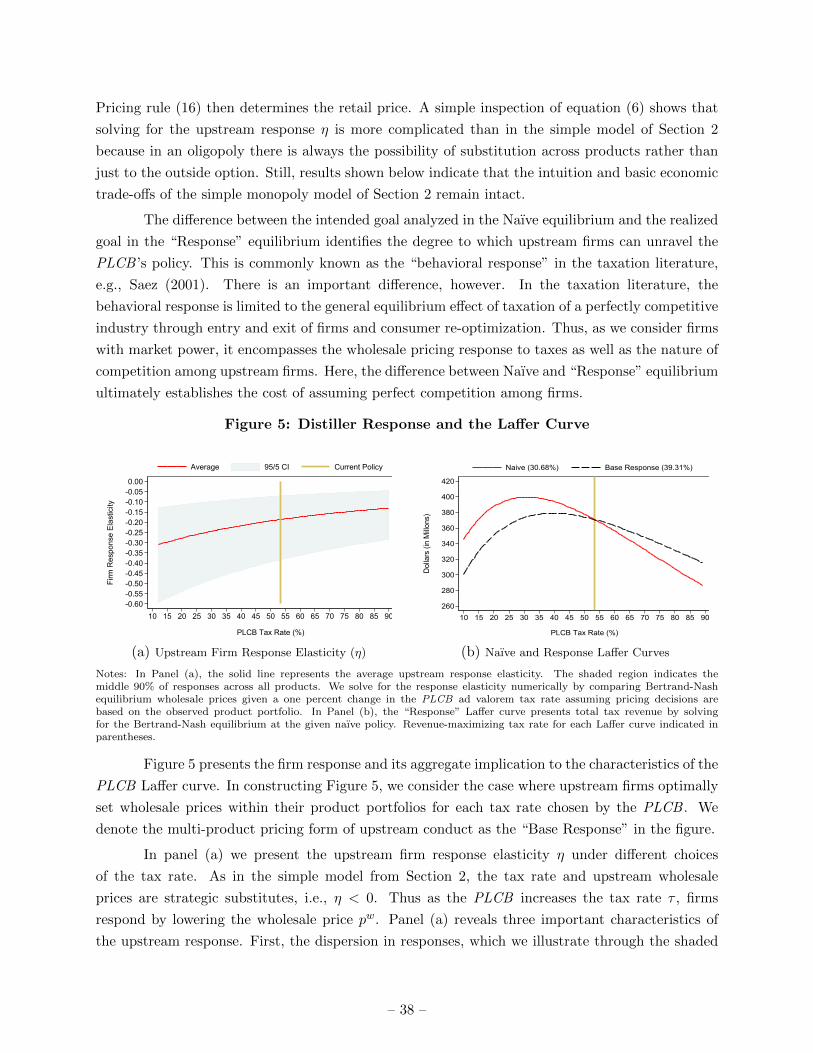
We show that market power among firms has a significant effect on the shape of the Laffer

curve. The estimated Laffer curve for a naıve policymaker is steeper than for the policymaker who

correctly anticipates pre-tax price responses. This is particularly true as conduct among upstream

becomes more collusive. Not accounting for the strategic response of upstream firms, therefore,

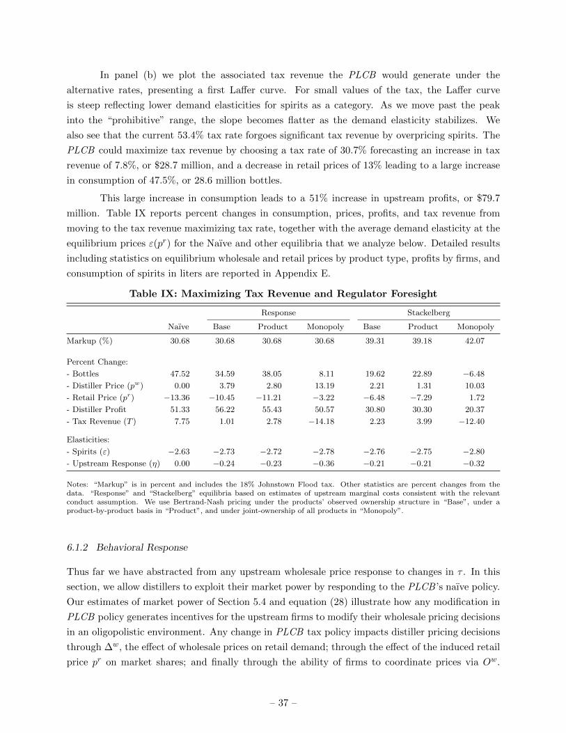
leads to poor policy recommendations. For instance, a naıve regulator would have concluded that

the state could increase tax revenues 7.75% (or $28.74 million) by reducing the ad valorem tax

from 53.4% to 30.68%. This reduction in the ad valorem tax would have increased profits for all

upstream firms, but we show that they could do even better by increasing their wholesale prices

by 3.79%, or 34 cents, on average. Thus, the estimated model indicates that upstream prices and

the tax rate are strategic substitutes – a prediction of the simple theoretical model.

– 2 –

While this change in upstream price may appear small, the fact that upstream distillers

price on the elastic region of demand leads to a large change in quantity demanded by consumers.

Ultimately, the firm response enables upstream firms to convert 87% of the incremental tax revenue

into firm profits, or equivalently the response limits the PLCB to attain only 13.8% of the forecasted

incremental revenues ($3.73 million). It is important to note that this substantial undoing of the

state’s revenue objective requires no coordination among firms. Were distillers to collude in setting

wholesale prices, choosing the naıve optimal tax rate leads to a net decrease in tax revenues of

14.18% of current revenue.

Alternatively, a regulator attempting to maximize tax revenue and endowed with perfect-

foresight would have predicted the upstream response and instead would only decrease the tax rate

to 39.31%, or 42.07% in the event of collusion among upstream firms. While the state does increase

tax revenue roughly two percent, profits among upstream distillers increase 30.8% as does their

share of integrated industry profits (from 29.5% to 34.9%).

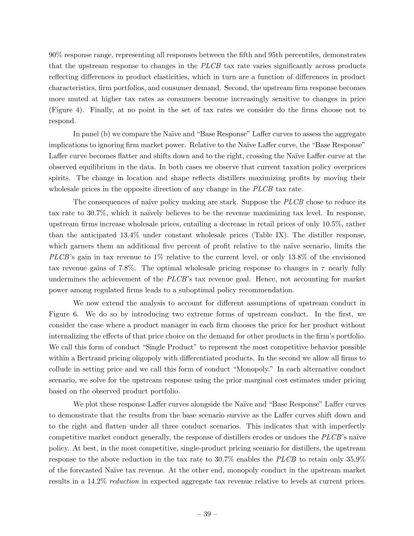
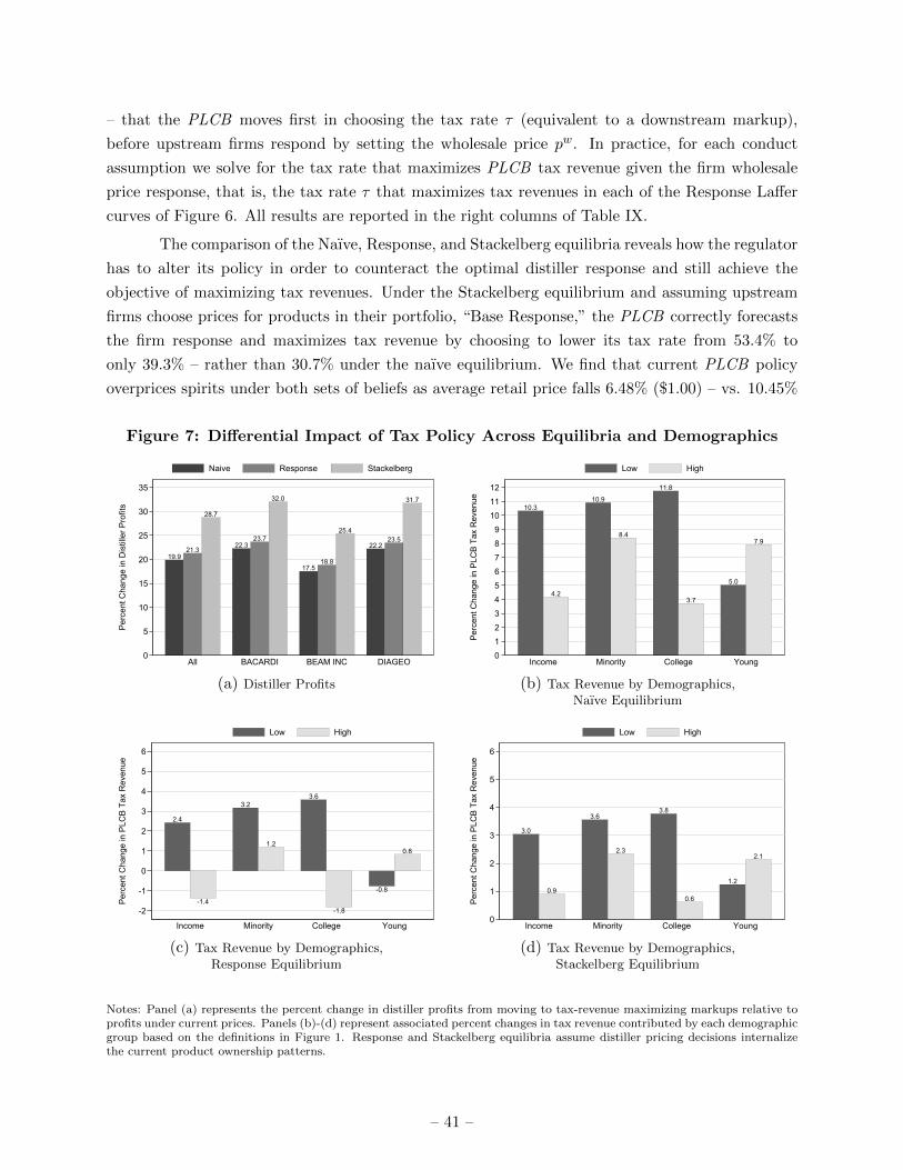
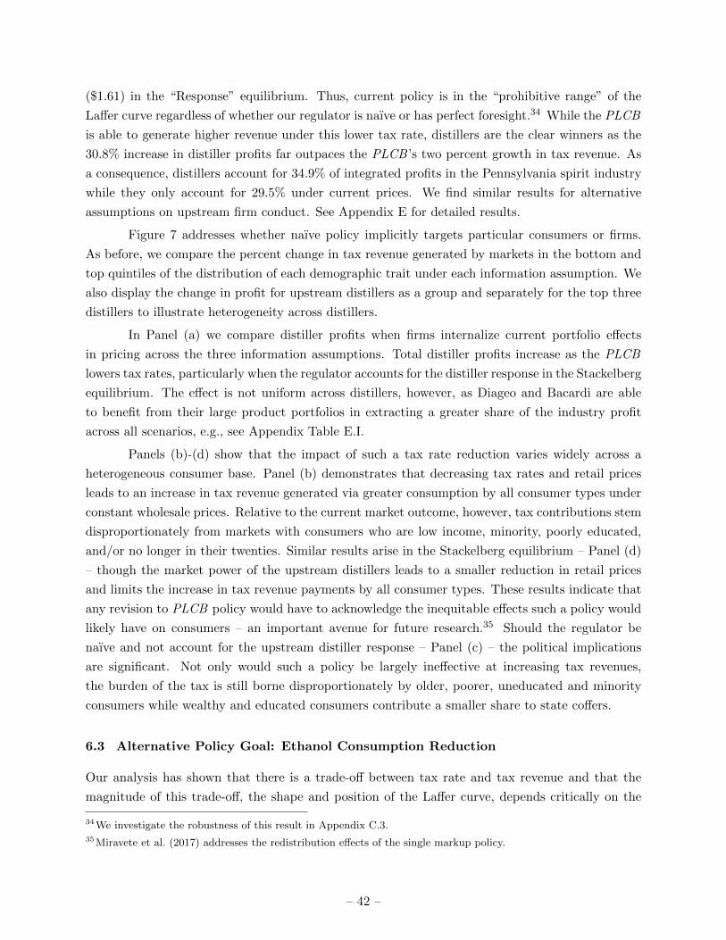
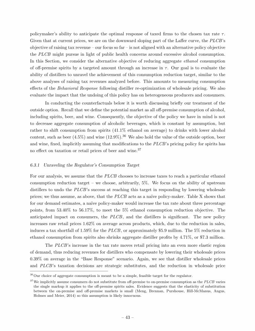
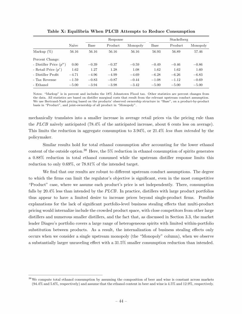
Finally, we show that the political ramifications of naıve policy – of assuming perfect compe-

tition among firms – are significant. Not only would such policy be largely ineffective at increasing

tax revenues, but the burden of the tax falls disproportionately on older, poorer, uneducated and

minority consumers. This highlights that the ability of policymakers to account for the responses of

firms and consumers to policies is of significance both from an equity and an efficiency standpoint.

It underscores the importance of recent efforts by, for example, the Congressional Budget Office

to consider Dynamic Scoring of new proposed legislation by accounting for the response of firms,

workers, and consumers to changes in government policy, a direct – albeit delayed – response to

the Lucas Critique. The major handicap then resides in correctly predicting how agents will react

to changes in fiscal policy across different industries.2

1.1 Related Literature

The current paper contributes to several strands of literature, including the characterization of the

Laffer curve, optimal taxation, the analysis of pass-through in non-competitive markets, and the

analysis of alcohol pricing regulation.

Theoretical analysis of the Laffer curve has fallen mostly within the reign of macroeconomics,

which has focused on the possibility of the Laffer curve arising as a result of a general equilibrium

effect induced by taxation on the supply of labor and capital.3 Early empirical attempts such as

Stuart (1981) or Fullerton (1982) build upon static two-sector general equilibrium models where

households allocate their time between taxed labor and non-taxed leisure. Pecorino (2011) adds

a dynamic component as hours worked entail human capital accumulation. Trabandt and Uhlig

(2011) allow for household preference heterogeneity within a neoclassical growth model to generate

2 See the presentation by Wendy Edelberg, the CBO’s Assistant Director for Macroeconomic Analysis, to the FederalReserve Bank of Chicago at https://www.cbo.gov/publication/50730.

3 See Ireland (1994), Novales and Ruiz (2002), or Schmitt-Grohe and Uribe (1997) to name a few.

– 3 –

labor and capital Laffer curves for the U.S. and fourteen European countries assuming calibrated

country-specific Frisch elasticities of labor supply and intertemporal elasticities of substitution.

Relative to this literature we focus on excise taxation with particular attention to the

responses of not only consumers but also suppliers with market power. Consequently within this

literature, our analysis is more related to optimal capital rather than labor taxation. Our results

then indicate that modifications of the capital tax rate could be largely undone by providers of

capital if they have market power – a likely scenario. The advantage of our approach is that we

have detailed industry data that allows us not to impose any restrictions on the model such as a

predetermined objective of the state. As our model generates robust estimates of consumer demand

and upstream market power, this approach increases the reliability of our conclusions.

We show that the existence, shape, and location of the Laffer curve in our context depends

not only on the interaction of the tax rate and consumers’ downstream product demand responses

(via demand elasticities) but also on upstream market power and firms’ strategic pre-tax price

setting. This is a commonly overlooked aspect of the analysis of taxation since the empirical public

finance literature deals primarily with perfectly competitive scenarios despite the well-documented

market power of firms in the studied industries.4 Our data enables us to evaluate this assumption by

drawing a distinction between the mechanical effects of and behavioral responses to taxation (Saez,

2001, §3.2). Specifically, we allow the policymaker to be well aware of downward sloping retail

demands but potentially naıve regarding the upstream firms’ reaction to taxes/pricing regulations.

A comparison of the Laffer curve with this naıve policy design to the one generated by a policymaker

who chooses the tax rate in anticipation of the optimal firm responses (Stackelberg equilibrium)

allows us to evaluate the implications of this assumption. Our results indicate that assuming perfect

competition among firms, i.e., assuming upstream firms cannot respond to changes in policy, has

substantial equilibrium effects on firms, consumers, and overall tax revenue across a variety of

assumptions regarding upstream conduct.5,6

Finally, we are not the first to address the implications of policy in the regulation of

alcoholic beverages. Seim and Waldfogel (2013) evaluate the potential welfare effects of free entry

in Pennsylvania. Aguirregabiria, Ershov and Suzuki (2016) study the case of partial entry in the

wine segment where state-run stores sell side by side with private, yet price regulated, retailers.

Illanes and Moshary (2015) take advantage of the privatization of the alcohol distribution system in

Washington state to evaluate the effect of potential retail entry on pricing and product offering. In

a related paper (Miravete, Seim and Thurk, 2017), we show that current policy is largely consistent

4 For instance, Chetty, Looney and Kroft (2009) and Evans, Ringel and Stech (1999) both assume competitive supplyin the beer and cigarette industries, respectively.

5 Weyl and Fabinger (2013) show the impact of imperfect competition on tax pass-through under a variety of modelenvironments but do not address asymmetric firms with horizontally-differentiated products. Consequently, ourresults provide an empirical extension.

6 There are other papers that address the market conduct in the alcoholic beverage industry. Conlon and Rao (2015)document how the “post and hold” regulation in some states help wholesalers set collusive prices. Miller andWeinberg (2015) use mergers in the brewing industry to identify collusive behavior.

– 4 –

with tax-revenue maximization (versus managing ethanol consumption) and compare the current

uniform policy to a subsidy-free taxation policy with optimal product-specific ad valorem taxes. We

find that the one-size-fits-all policy employed by the state generates significant redistribution within

upstream firms and downstream consumers. Griffith, O’Connell and Smith (2017) evaluate the use

of product-specific corrective taxes to minimize health externalities related to ethanol consumption

under the assumption that all firms, including suppliers and retailers, do not respond. In this paper,

we abstract from modeling the motivation behind the state’s tax code to more clearly illustrate the

key determinants of the tax rate/revenue trade-off and to characterize the shape and location of

the Laffer curve empirically while accounting for re-optimization by both firms and consumers.

1.2 Organization of the Paper

The paper is organized as follows. In Section 2 we provide a simple model of taxation under

imperfect competition to illustrate the key mechanisms underlying our results. In Section 3 we

present the data, discuss the details of the Pennsylvania pricing rule, address the interaction with

the upstream distillers, and document heterogeneous consumption patterns across demographic

groups. In Section 4 we present an equilibrium discrete choice model of demand for horizontally

differentiated spirits. The model allows preferences to be correlated across products of similar

characteristics and incorporates the features of the current pricing regulations while allowing for

(but not imposing) imperfect competition in the upstream distillery market. In Section 5 we discuss

the estimation procedure and how the unique features of our data help identify the rich substitution

patterns across products in our econometric specification. We pay particular attention to dealing

with the potential endogeneity of prices using retail price information from other control states and

variation in input costs. We also show how we use the estimated model to infer upstream market

power among distillers. In Section 6 we show that this market power has significant implications

for the shape and location of the Laffer curve while also documenting the variation in Laffer curves

across consumer types. We conclude and discuss avenues for future research in Section 7. We

include additional data sources, descriptive statistics, robustness of demand estimates, and other

results in the Appendices.

2 A Simple Model of the Laffer Curve Under Market Power

In this section we present a simple model of monopoly excise taxation to provide an economic

framework for the interpretation of our empirical analysis in an oligopolistic environment. Our goal

is to illustrate how a regulator’s tax rate choice affects its tax revenue when allowing for optimal

price responses by taxed firms to changes in policy. We show that tax revenue is not monotonic in

the tax rate and that certain tax rates fall into what Arthur Laffer called the “Prohibitive Range,”

when an increase in the tax rate leads to a reduction in tax revenue. To this end, we investigate how

the optimal pre-tax price responds to a change in the tax rate, and show that whenever demands are

less convex than in the isoelastic case, the pre-tax price and the tax rate are strategic substitutes.

– 5 –

Consider the case of a single product sold by a monopoly supplier and produced at a constant

marginal cost. Focusing on the single-product monopoly case allows us to avoid accounting for

cross-product substitution as the excise tax and tax-inclusive prices change; instead we simply

consider the marginal consumer’s decision to switch between the inside and outside good. Our

empirical analysis in the context of multi-product oligopoly upstream suppliers agrees, nevertheless,

with all predictions of the model. The monopolist chooses the pre-tax price pw (wholesale price

in our empirical context) for a given tax rate τ ≥ 0, which impacts the tax-inclusive price the

consumer pays, pr (retail price),

pr = (1 + τ)pw . (1)

In setting its optimal pre-tax price, the monopolist chooses pw to maximize profits Π(pw) = (pw −c)D(pr), given the retail demand D(pr), constant marginal cost c, and the chosen tax rate τ , which

requires:

D(pr) + (pw − c)D′(pr)(1 + τ) = 0 , (2)

or equivalently, in terms of the Lerner index,

pw − cpw

=−D(pr)

D′(pr)(1 + τ)· 1 + τ

pr=−1

ε(pr). (3)

This inverse-elasticity pricing rule relates the pre-tax (wholesale) markup of the monopolist

to the inverse of the demand elasticity evaluated at the tax-inclusive (retail) price. The monopolist

thus sets the pre-tax price pw so that the tax-inclusive price falls in the elastic region of demand.

This result is behind the optimal pricing response of the taxed firm to changes in the tax rate

shown below. We argue that under general conditions, for any demand that is less convex than an

isoelastic demand function, a tax rate increase induces the non-competitive taxed firm to reduce

its pre-tax price in order to keep the tax-inclusive market price in a region of demand that is not

too elastic. Thus, tax rates and non-competitive firm prices move in opposite directions, i.e., they

are strategic substitutes.

To characterize the monopolist’s optimal price response to a change in tax policy we make

use of the retail price definition in equation (1) and totally differentiate the first order condition in

equation (2) with respect to pw and τ to obtain:

dpw

dτ=−1

1 + τ· (2pw − c)D′(pr) + pr(pw − c)D′′(pr)

2D′(pr) + (pw − c)(1 + τ)D′′(pr). (4)

For convenience we define η(τ) as the elasticity of the monopolist’s optimal pre-tax price to a

change in the tax rate τ . We make use of the inverse-elasticity rule (3) to express the firm’s

optimal response elasticity as

η(τ) ≡ dpw

dτ· τpw

=−1

1 + τ·

(pw − pw

ε(pr)

)D′(pr)− pw×pr

ε(pr) D′′(pr)

2D′(pr)− pr

ε(pr)D′′(pr)

· τpw

. (5)

– 6 –

Further simplification using the retail price definition (1) yields:

η(τ) =−τ

1 + τ·

(1− 1

ε(pr)

)− κ(pr)

2− κ(pr), (6)

where κ(pr) is the curvature of demand given by

κ(pr) =D′′(pr)D(pr)

[D′(pr)]2. (7)

The curvature of demand κ(pr) is the key element that determines the sign of η(τ). We are

interested in characterizing demand conditions under which the pre-tax price response elasticity

η(τ) is negative, given that the firm prices in the elastic region of demand, ε(pr) < −1. We explore

first the case of linear and concave demand followed by somewhat convex demand functions.

It is straightforward to show that η(τ) < 0 in equation (6) under profit-maximizing pricing

with ε(pr) < −1 whenever demand is linear or concave as D′′(pr) ≤ 0 ensures that κ(pr) ≤ 0. Linear

demand is commonly used for algebraic convenience but concave demand is frequently assumed in

theoretical models, see Tirole (1989, §1.1).

There is however a larger set of demand systems that entails the strategic substitutability

of pw and τ . For instance, equation (6) indicates that η(τ) is always negative when κ(pr) ∈ [0, 1)

and the monopolist prices on the elastic region of demand. The curvature condition of κ(pr) < 1

describes the class of log-concave demand functions, including both concave and somewhat con-

vex demand functions.7 Log-concavity characterizes the vast majority of demand specifications

commonly used in economic analysis, including discrete choice models of demand based on Type

I extreme value distributed errors so widely used in empirical work, including ours, e.g., Fabinger

and Weyl (2016, Appendix 3).

Even for demand systems with higher curvature, with κ(pr) ∈ [1, 2), it is possible for η(τ)

to be negative, depending on the relative magnitudes of(1− 1

ε(pr)

)and κ(pr).8 Isoelastic demand, a

popular choice in the macro literature (e.g., Dixit-Stiglitz CES preferences), amounts to a limiting

case as it is straightforward to show that for these demand functions κ(pr) =(

1− 1ε(pr)

)and

thus, η(τ) = 0 according to equation (6). Thus, firms in these models do not alter their pricing

decisions in response to changes in tax policy by assumption. But whenever demand is less convex

than this popular limiting case, we characterize a large and empirically relevant class of demand

specifications where the optimal response of the monopolist to an increase in the tax rate always

is to reduce the pre-tax price, i.e., η(τ) < 0 so that the pre-tax prices and tax rates are strategic

substitutes.

7 If κ(pr) < 1, it follows from the definition of curvature that D′′(pr)D(pr) − [D′(pr)]2 < 0, which is the conditionfor demand to be log-concave.

8 We restrict attention to demand systems with κ < 2 since κ(pr) ∈ [0, 2) ensures that the revenue function R(pr) =prD(pr) is concave in pr, or equivalently, that the marginal revenue function is decreasing, a common demandrestriction in models of imperfect competition.

– 7 –

We can now explore how total tax revenue collected by the government varies as a function

of the tax rate τ when we account for the firm’s optimal price response. The government tax

revenue function is given by

T (τ) = (pr − pw)D(pr) = τpwD((1 + τ)pw

), (8)

where pr and pw are implicit functions of τ , pr(τ) and pw(τ), through the definition of the tax-

inclusive price (1) and the pre-tax price response elasticity (6). The effect of a change in the tax

rate on government tax revenue is

dT (τ)

dτ= pwD(pr) + τpwD′(pr)pw +

dpw

dτ

(τD(pr) + τpwD′(pr)(1 + τ)

)

= pw(D(pr) + τpwD′(pr)

)+ η(τ)pw

(D(pr) + ε(pr)D(pr)

)

= pwD(pr)

[(1 +

τ

1 + τε(pr)

)+ η(τ)

(1 + ε(pr)

)]. (9)

Note that the sign of dT (τ)/dτ is ambiguous and depends on the relative magnitudes of

the tax rate, demand elasticity, and the pre-tax price response elasticity. The prohibitive range of

the Laffer curve arises for a given tax rate τ when the equilibrium price elasticity of demand ε(pr)

and the equilibrium pre-tax price response elasticity η(τ) are such that:

dT (τ)

dτ< 0 ⇐⇒ 1 +

τ

1 + τε(pr) + η(τ)

(1 + ε(pr)

)< 0 . (10)

When are tax, demand, and upstream conduct conditions such that equation (10) is sat-

isfied? We consider first the case of a naıve policymaker who mistakenly believes that – akin to

the case of perfect competition – the monopolist will not modify its pre-tax (wholesale) price in

response to an increase in the ad valorem tax rate τ . When η(τ) = 0, condition (10) will not hold

for sufficiently low τ . However, this condition eventually holds as τ increases by reducing the total

value of sales receipts as higher tax rates push the price pr into a more elastic region of demand

for all demand systems other than the isoelastic limiting case. The macro literature relies on a

similar incentive mechanism to generate a Laffer curve: higher income taxation reduces workers’

labor supply to eventually reduce the labor tax base and income tax revenues. See Trabandt and

Uhlig (2011, Proposition 2).

Rewriting equation (9) when η(τ) = 0 shows that all we require to be on the prohibitive

region of the Laffer curve under a naıve policymaker is that consumer demand is sufficiently elastic

at the tax-inclusive equilibrium price,

ε(pr(τ)) < ε◦(τ) = −1 + τ

τ, (11)

– 8 –

For instance, for a tax rate of 50% (similar to the 53.4% tax charged by the PLCB) to be in the

prohibitive region of the Laffer curve of a naıve policymaker, the demand elasticity ε(pr) at the

corresponding equilibrium tax-inclusive price needs to be lower than ε◦(0.5) = −3 (a value that

many of our demand estimates exceed). The higher the tax rate and thus final retail prices, the less

elastic demand needs to be to reach the prohibitive range of the Laffer curve. Thus, tax revenue will

fall if a naıve policymaker increased taxes from a starting tax rate of 70% and the good’s demand

elasticity at the equilibrium price is at least ε(pr) < ε◦(0.7) = −2.43. Conversely, for many, more

moderate, taxation schemes, such as sales taxes, which in the U.S. across states reach only 9.45%

in 2015, demand for the affected products is unlikely to be sufficiently elastic for the observed tax

rates to be near or beyond the peak of the Laffer curve.9

To complete the analysis we compare the features of the Laffer curve for a naıve policymaker

described above with that of a policymaker with perfect foresight, capable of anticipating how the

monopolist re-optimizes its pricing decision after a change of the tax rate. Substituting (6) for η(τ)

in condition (10), the prohibitive range of the Laffer curve arises when

2− κ(pr) + 2τ

τ+ ε(pr) +

1

ε(pr)< 0 . (12)

For this inequality to hold over the elastic range of demand, ε < −1, it suffices that

ε(pr) < ε?(τ, κ) = −2− κ(pr) + τ

τ. (13)

How does the implicit relationship between the tax rate and the elasticity of demand that entails

a tax rate beyond tax revenue maximizing levels compare to the above, when η(τ) = 0? A general

comparison is dependent on the chosen demand system, which dictates a choice of κ(pr) and ε(pr).

However, when demand is log-concave and κ(pr) ∈ [0, 1), as in our empirical setting, we can show

that for any given tax rate τ :

ε?(τ, κ) = −2− κ(pr) + τ

τ< −1 + τ

τ= ε◦(τ) . (14)

When allowing for a strategic response by the monopolist to chosen tax rates, demand at tax-

inclusive retail prices thus needs to be more elastic than under the naıve scenario for any particular

tax rate to push tax revenues down the slippery slope of the Laffer curve. For example, for the above

tax rate of 50% to be in the prohibitive region for a policymaker with perfect foresight, demand

at the resulting tax-inclusive prices needs to be more elastic than −5 or −4 for κ(τ) equal to 0 or

0.5, respectively. This compares to the above critical value for the elasticity of −3 when η(τ) = 0.

For a given tax rate, the difference between the elasticity cutoff values for the perfect foresight and

naıve cases converges to zero as demand becomes more convex, reflecting that ε?(τ, κ)→ ε◦(τ) as

κ(pr)→ 1, and is highest when demand is linear and κ(pr) = 0.

9 See https://taxfoundation.org/state-and-local-sales-tax-rates-2015/. A rate of τ = 10% falls beyond thepeak of the Laffer curve if the demand elasticity at tax inclusive prices would need to be smaller than −11.

– 9 –

The flip side of this result is that a policymaker with perfect foresight may need to set a

higher tax rate to maximize tax revenues when compensating for the reduction in pre-tax price by

the monopolist, η(τ) < 0, than the naıve policymaker would have chosen. Expressing equation (14)

in terms of the optimal tax rate that maximizes tax revenue given the demand responsiveness at

the tax-inclusive prices, we have that

τ?(ε, κ) = −2− κ(pr)

1 + ε(pr)> − 1

1 + ε(pr)= τ◦(ε(pr)) (15)

Note that τ◦(ε) is not necessarily equal to τ◦(ε), the tax revenue maximizing tax rate for

the naıve policymaker, since the demand elasticities are evaluated at different tax-inclusive retail

prices, pr = (1 + τ?)pw in the case of the sophisticated policymaker and pr = (1 + τ◦)pw for the

naıve case. Locally, with small changes in the tax-inclusive retail price, however, and supported

by the empirical evidence we present below, the difference between τ◦(ε) and τ◦(ε) is sufficiently

small that τ?(ε, κ) > τ◦(ε(pr)).

Moving from the naıve scenario, η(τ) = 0, to one where the policymaker has perfect

foresight, η(τ) < 0, not only tends to shift the Laffer curve to the right, but also makes it flatter.

This is evident when inspecting the last term in equation (9), η(τ)(1+ε(pr)

)> 0, which equals zero

in the naıve scenario. This is the case because of the strategic substitutability of the tax rate and

wholesale prices, η(τ) < 0, under perfect foresight and the monopolist’s optimal pre-tax pricing on

the elastic region of demand, 1 + ε(pr) < 0. Thus, the stronger the firm response, the flatter the

slope of the Laffer curve becomes.

In summary, the theoretical model suggests that the downward sloping part of the Laffer

curve arises if demand is sufficiently elastic relative to the tax rate and the elasticity of the pricing

response of the taxed firm to changes in the tax policy. Even for the monopoly case, empirical

analysis is needed to determine the elasticity of demand under alternative tax-inclusive prices and

characterize the effective tax revenue function. Similarly, accounting for the firm’s price response

to excise taxation, which implies a possible shift and flattening of the Laffer curve relationship

between tax rates and revenue, requires estimates of firm market power via η(τ) and the slope of

consumer demand via ε(pr). Our analysis of PLCB pricing of spirits allows us to empirically assess

the necessary equilibrium responses of upstream firms and consumers.

This analysis could be extended to various homogeneous good oligopoly models along the

lines of the framework for analyzing tax incidence put forward by Weyl and Fabinger (2013). In our

context, however, the PLCB deals with horizontally-differentiated products for which theoretical

results do not exist, e.g., Fabinger and Weyl (2016, Appendix E). The main difficulty in evaluating

the effect of a tax rate increase in this context is that it not only induces substitution to the outside

option but also to other products that are taxed and therefore also generate tax revenues. In

consequence, addressing our research objective requires evaluating the determinants of the Laffer

curve empirically, accounting for the fact that the overall change in tax revenue after a change in the

tax rate reflects unequally induced changes in product sales due to heterogeneity in product costs

– 10 –

and characteristics. Further, firms and consumers can respond differently to a tax rate change based

on differences in market power and heterogeneous preferences, respectively. We account for these

effects empirically in characterizing the Laffer curve across not just one, but all spirits products,

both in aggregate and for different consumer types. In doing so, we are particularly interested in

comparing the tax revenue expected by a naıve regulator who mistakenly neglects the ability of

firms to re-optimize after a tax change, η(τ) = 0, to that realized by a policymaker who correctly

anticipates firm responses to its actions, η(τ) < 0.

3 PLCB Pricing and Sales Data

In this section we describe our data and institutional details that inform our theoretical modeling

and econometric specification. We first describe the data we obtained from the state of Pennsylvania

and other sources on the sales, prices, and characteristics of all products sold through the state-run

network of stores. We then summarize Pennsylvania’s current pricing regulations of alcoholic bev-

erages. We document how upstream firms’ pricing is constrained by rules regarding the frequency

and duration of temporary wholesale price adjustments. The fact that distillers need to decide far

in advance when to put their products on sale temporarily significantly reduces the endogeneity

concerns common in the estimation of models of demand for differentiated products. Next, we

explore the nature of competition in the upstream distiller market that mitigates the effectiveness of

any tax/pricing policy adopted by the PLCB . Finally, we document the heterogeneity of consumer

preferences for different types of spirits, a key source of identification in our empirical strategy.

3.1 Data: Quantities Sold, Prices, and Characteristics of Spirits

We obtained store-level panel data from the Pennsylvania Liquor Control Board (PLCB) under

the Pennsylvania Right-to-Know Law. The data contain daily information on quantities sold and

gross receipts at the UPC and store level for all spirits and wines carried by the PLCB from 2002

to 2004. We chose this sample because there were no mergers or acquisitions of relevance in the

upstream distiller industry segment resulting in a stable competitive environment. As a result,

pricing follows the “normal” pattern contemplated in the PLCB ’s rules. In addition, we received

information on the wholesale price of each product. These wholesale prices are constant across

stores, but vary over time according to well defined pricing periods.

As of January of 2003, the PLCB operated a system of 593 state-run retail stores spread

across the state.10 We combine sales of stores in the same zip code and drop several wholesale and

outlet stores, resulting in a total of 456 local markets. We then match combined store purchases with

consumer demographics by linking store locations with data on local population and demographic

characteristics using the 2000 Census. The PLCB opened and closed several stores over the time

10See Seim and Waldfogel (2013, §2) for a detailed account of the welfare losses induced by the very limited entryallowed in the wine and spirit segment of the Pennsylvania market. Pennsylvania also has a private system for thesale of beer, allowing the controlled entry of private retailers.

– 11 –

period of our sample. We take these entry/exit decisions as exogenous shifts in the demographic

composition of the potential pool of customers of each store. This feature of the data helps in

identifying the demographic interactions in our estimated model.11

Each store carries a multitude of wine and spirit products. We focus on the spirits category

as it represents a majority of PLCB off-premise sales, 60.8% of store revenue. These products

further constitute a well-defined and mature product category that can be described by few, easily

measurable product characteristics, including the type of spirit, the alcohol content, whether or not

a fruit or other flavor is added, and whether or not the product is imported.12

We further focus on sales of popular 375 ml, 750 ml, and 1.75 L bottles of products in the

spirits category, representing 80.9% of total spirit category sales by volume and 91.6% by revenue.

The resulting sample exhibits a long right tail common to consumer goods, where many products

are available to consumers but are rarely purchased. We therefore restrict the sample to only include

the most popular products in each bottle size, spirit type pairing. Consequently, a 750 ml bottle of

E&J Brandy (average retail price of $9.95) is in our final sample while a 750 ml bottle Remy Martin

Louis XIII Cognac (average retail price of $1,078) is not.13 Our final sample consists of 3,377,659

observations of market and time-period level purchases of 312 products that span brandy, cordials,

gin, rum, vodka, and whiskey for three bottle sizes. The final sample represents 56.8% and 63.2%

of the total off-premise bottle sales and revenue from spirits, respectively.

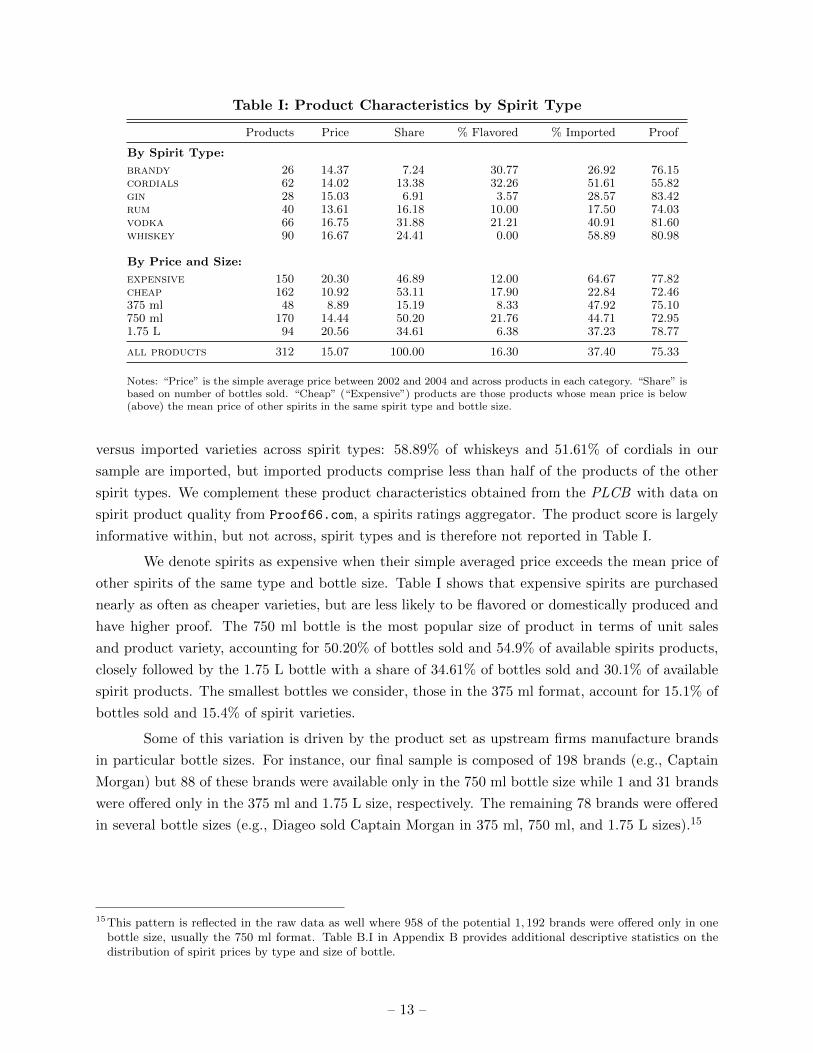
Table I reports the average characteristics of products in our sample. The average proof

is 75.33; 37.40% of products are imported; and 16.3% of products contain flavor add-ins.14 Table

I summarizes these product characteristics further by type of spirit. Vodkas and whiskeys have

significantly larger market shares (31.88% and 24.41%, respectively) than rum (16.18%), cordials

(13.38%), brandy (7.24%), or gin (6.91%). The differences in product variety within each category

mirror the differences in market shares, with only approximately one half as many brandy and

gin varieties as vodkas while 28.9% of the products are whiskeys. Flavored products are primarily

cordials and brandies and to a lesser extent vodkas and rums. We also see variation in domestic

11Appendix A describes how we assign Census block groups to their closest store and how we deal with store openingsand closings, and provides detail on the construction of the demographic variables. We also document that thelarge majority of spirits are sold at every store; this alleviates concerns about assortment differences between storesleading to potential competition for consumers between stores.

12This contrasts favorably with wines whose quality determinants are mostly unobserved, with a large number ofproducts with limited life cycles. This leads to tiny, highly volatile market shares of wines with frequent entry andexit of products of different vintages. For example, within the popular 750 ml bottle category, the top-100 sellingwines (out of 4,675) constitute 45% of total 750 ml wine revenue.

13We define popular products as the highest selling products that together account for 80% of total off-premise spiritsales of a bottle size, spirit type pair. By this definition, a 375 ml bottle of Captain Morgan could theoretically beexcluded from the sample, if it sales rank among 375 ml bottles is too low, while the 750 ml and 1.75 L versionsare included. In practice this did not occur. We also drop the Tequila segment as it accounts for few products.Together, these two restrictions allow us to drop a total of 1,240 products from our sample.

14 In 16th century England, if a pellet of gunpowder soaked in a spirit could still burn determined whether the spiritwas “proof” and thus taxed at a higher rate. Only if the alcohol by volume in rum exceeds 57.15% will gunpowderignite. To simplify, since 1848 in the U.S., a 100 proof corresponds to a spirit with 50% alcohol by volume content.See Jensen (2004).

– 12 –

Table I: Product Characteristics by Spirit Type

Products Price Share % Flavored % Imported Proof

By Spirit Type:

brandy 26 14.37 7.24 30.77 26.92 76.15cordials 62 14.02 13.38 32.26 51.61 55.82gin 28 15.03 6.91 3.57 28.57 83.42rum 40 13.61 16.18 10.00 17.50 74.03vodka 66 16.75 31.88 21.21 40.91 81.60whiskey 90 16.67 24.41 0.00 58.89 80.98

By Price and Size:

expensive 150 20.30 46.89 12.00 64.67 77.82cheap 162 10.92 53.11 17.90 22.84 72.46375 ml 48 8.89 15.19 8.33 47.92 75.10750 ml 170 14.44 50.20 21.76 44.71 72.951.75 L 94 20.56 34.61 6.38 37.23 78.77

all products 312 15.07 100.00 16.30 37.40 75.33

Notes: “Price” is the simple average price between 2002 and 2004 and across products in each category. “Share” isbased on number of bottles sold. “Cheap” (“Expensive”) products are those products whose mean price is below(above) the mean price of other spirits in the same spirit type and bottle size.

versus imported varieties across spirit types: 58.89% of whiskeys and 51.61% of cordials in our

sample are imported, but imported products comprise less than half of the products of the other

spirit types. We complement these product characteristics obtained from the PLCB with data on

spirit product quality from Proof66.com, a spirits ratings aggregator. The product score is largely

informative within, but not across, spirit types and is therefore not reported in Table I.

We denote spirits as expensive when their simple averaged price exceeds the mean price of

other spirits of the same type and bottle size. Table I shows that expensive spirits are purchased

nearly as often as cheaper varieties, but are less likely to be flavored or domestically produced and

have higher proof. The 750 ml bottle is the most popular size of product in terms of unit sales

and product variety, accounting for 50.20% of bottles sold and 54.9% of available spirits products,

closely followed by the 1.75 L bottle with a share of 34.61% of bottles sold and 30.1% of available

spirit products. The smallest bottles we consider, those in the 375 ml format, account for 15.1% of

bottles sold and 15.4% of spirit varieties.

Some of this variation is driven by the product set as upstream firms manufacture brands

in particular bottle sizes. For instance, our final sample is composed of 198 brands (e.g., Captain

Morgan) but 88 of these brands were available only in the 750 ml bottle size while 1 and 31 brands

were offered only in the 375 ml and 1.75 L size, respectively. The remaining 78 brands were offered

in several bottle sizes (e.g., Diageo sold Captain Morgan in 375 ml, 750 ml, and 1.75 L sizes).15

15This pattern is reflected in the raw data as well where 958 of the potential 1, 192 brands were offered only in onebottle size, usually the 750 ml format. Table B.I in Appendix B provides additional descriptive statistics on thedistribution of spirit prices by type and size of bottle.

– 13 –

3.2 The Mechanics of the Pricing Regulation

The PLCB acts as a monopolist in the retail distribution of wine and spirits where the Pennsylvania

State Legislature exerts regulatory oversight over several aspects of the daily operations of the

stores. Most notably, as per the Pennsylvania Liquor Code (47 P.S. §1-101 et seq.) and the

Pennsylvania Code Title 40, the legislature imposes a uniform markup rule upon the retail prices

the PLCB charges both across products and across stores. Prices of spirits are thus identical across

the state at a point in time and follow a common pricing/taxation rule known to all consumers and

upstream manufacturers.

This rule has been modified only infrequently over the years. From 1937 until 1980, the

retail price for all products was based on a 55% markup over wholesale cost for all gins and whiskeys

and 60% markup for other spirits. In 1980, the markup was reduced to 25% for all products and

a per-unit handling fee, the Logistics, Transportation, and Merchandise Factor (LTMF ), of $0.81

was introduced and later increased to $0.85 in 1982. The agency instituted the current 30% markup

in 1993 when it also modified the unit fee to vary by bottle size to better reflect transportation

costs from the PLCB ’s centralized warehouses to the retail stores. The LTMF unit fee for the

375 ml, 750 ml, and 1.75 L bottles in our sample amounts to $1.05, $1.20, and $1.55, respectively.

For the average product, the LTMF fee accounts for 26.7% of the final retail markup. In addition,

consumers also have to pay an 18% sales tax, the “Johnstown Flood Tax,” on all liquor purchases.16

Accordingly, the retail price pr of a given product with wholesale price, pw, is calculated as:17

pr = [pw × 1.30 + LTMF ]× 1.18 . (16)

Of primary concern for this paper is the uniform markup, an ad valorem tax, applied to all products,

amounting to (1.30× 1.18− 1), or 53.4%.

The PLCB has limited ability to depart from this uniform percent markup rule. It operates

seven outlet stores close to the state’s borders, in an effort to address any border bleed of consumers

who illegally import lower-priced products into Pennsylvania from neighboring states. While these

stores offer wines and spirits at discounted prices, the PLCB remains within the uniform markup

policy by selling products in the outlet stores not found in regular stores, for example multi-packs

or unusual bottle sizes for a particular product. Controlling for these stores has little qualitative

or quantitative effects on our results. Related robustness checks are reported in Appendix C.1.

The PLCB purchase bottles of spirits directly from upstream distillers at wholesale prices

pw. Because of the legislated pricing formula, retail price pr is driven by the wholesale pricing

decisions pw of the PLCB ’s suppliers and any change in the wholesale price results in a change

to the retail price passed on to consumers. A new product’s wholesale price remains fixed for

16The original 10% tax was instituted in 1936 to provide $41 million for the rebuilding of the flood-ravaged town ofJohnstown. Despite reaching the funding goal after the initial six years, the tax was never repealed, but insteadrose twice to 15% in 1963 and to 18% in 1968.

17An additional 6% sales tax is then applied to the posted price to generate the final price paid by the consumer.

– 14 –

one year after its introduction. For mature products, distillers can modify the wholesale price they

charge the PLCB at set intervals called “pricing periods” which last four or five weeks and typically

coincide with the month of year. We can therefore aggregate daily data on prices and quantity

sold to the level of these pricing intervals without concern of introducing aggregation bias into our

demand estimates – a useful aspect of our data.

The PLCB places some limitations on how often distillers can change the wholesale price for

mature products. Temporary wholesale price changes, typically price reductions or sales, amount

to 84.8% of price changes in our sample. Distillers can temporarily adjust their wholesale prices up

to four times a year, or once per quarter, but need to submit such proposed price changes to the

PLCB at least five months before the start of the promotion. A product can thus go on sale for

one month, but not for two in a row.

Upstream firms can also permanently change the wholesale price of a product, i.e., a change

in the reference price for temporary price changes. A permanent price change takes place at the

beginning of four-week long reporting periods which, for accounting purposes, occur at a slightly

different periodicity than the pricing periods. These price changes are instituted at the beginning

of the quarter’s first full reporting period, with some discretion on the part of the PLCB as to

the choice of actual reporting period. There is a time lag, however: distillers have to submit the

request for a permanent price increase by the start of the previous quarter. Permanent wholesale

price decreases may be submitted at any time and take effect at the beginning of the next period.

We discuss the periodicity of the price series further in Appendix A. The pricing periods we use

in our analysis below follow the periodicity of sales, resulting in 34 periods from 2002 to 2004.

Note that the delay between the request and effectiveness of either permanent or temporary price

adjustments limits the ability of the distillers to respond to temporary demand shocks – an issue

we revisit when discussing price endogeneity concerns in Section 5.

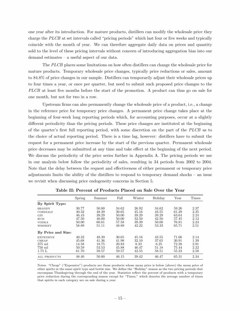
Table II: Percent of Products Placed on Sale Over the Year

Spring Summer Fall Winter Holiday Year Times

By Spirit Type:

brandy 30.77 50.00 34.62 26.92 34.62 59.26 2.37cordials 40.32 48.39 30.65 45.16 43.55 61.29 2.35gin 46.43 39.29 50.00 39.29 39.29 63.64 2.24rum 47.50 40.00 50.00 32.50 42.50 57.45 2.12vodka 50.00 60.61 57.58 39.39 50.00 76.81 2.24whiskey 58.89 51.11 48.89 42.22 53.33 65.71 2.51

By Price and Size:

expensive 40.32 48.39 30.65 45.16 43.55 71.66 2.14cheap 45.68 41.36 41.98 32.10 37.65 30.91 1.39375 ml 14.58 18.75 20.83 8.33 6.25 72.28 2.91750 ml 50.59 53.53 45.88 46.47 51.18 75.44 2.221.75 L 61.70 59.57 59.57 42.55 58.51 55.23 2.50

all products 48.40 50.00 46.15 39.42 46.47 65.31 2.34

Notes: “Cheap” (“Expensive”) products are those products whose mean price is below (above) the mean price ofother spirits in the same spirit type and bottle size. We define the “Holiday” season as the two pricing periods thatencompass Thanksgiving through the end of the year. Statistics reflect the percent of products with a temporaryprice reduction during the corresponding season except for “Times,” which denotes the average number of timesthat spirits in each category are on sale during a year.

– 15 –

Table II presents descriptive statistics for changes in temporary price. First, distillers

temporarily change a product’s price 2.3 times a year on average. While not all products experience

a temporary price change, the majority do; 65.31% of spirits are on sale at least once in a given

year. This is true across spirit types, with distillers changing the price of vodkas, expensive varieties,

and all but the largest bottles more frequently than the rest. There is also a seasonal pattern of

price changes across spirit types as distillers are more likely to change a product’s price during

the Summer and less likely during the Winter. Over the holidays, defined as pricing periods that

overlap with Thanksgiving through the end of the year, distillers place 46.47% of our spirit products,

ranging from 34.62% of brandies to 53.33% of whiskeys, on sale at least once, but change the price

of 375 ml bottles rarely. The combination of variation in monthly price changes, both temporary

and permanent, and differences in the amount of the price changes is the primary source of price

variation that we exploit in the estimation of our demand model.

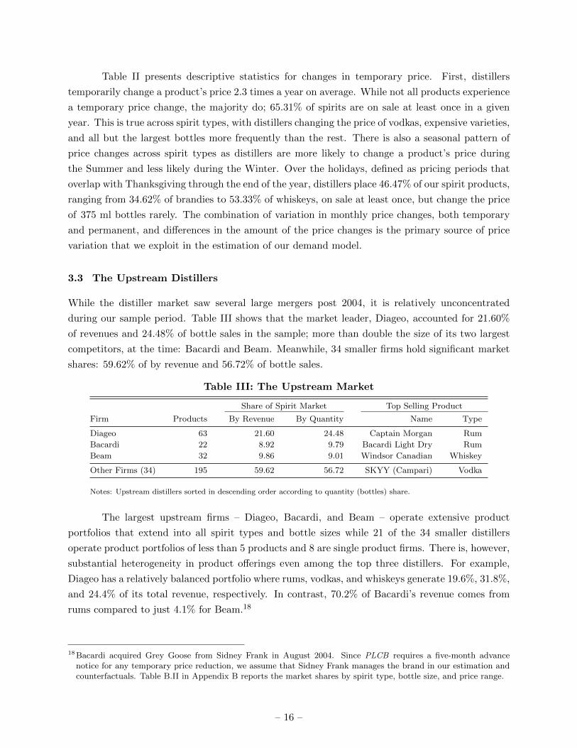
3.3 The Upstream Distillers

While the distiller market saw several large mergers post 2004, it is relatively unconcentrated

during our sample period. Table III shows that the market leader, Diageo, accounted for 21.60%

of revenues and 24.48% of bottle sales in the sample; more than double the size of its two largest

competitors, at the time: Bacardi and Beam. Meanwhile, 34 smaller firms hold significant market

shares: 59.62% of by revenue and 56.72% of bottle sales.

Table III: The Upstream Market

Share of Spirit Market Top Selling Product

Firm Products By Revenue By Quantity Name Type

Diageo 63 21.60 24.48 Captain Morgan Rum

Bacardi 22 8.92 9.79 Bacardi Light Dry Rum

Beam 32 9.86 9.01 Windsor Canadian Whiskey

Other Firms (34) 195 59.62 56.72 SKYY (Campari) Vodka

Notes: Upstream distillers sorted in descending order according to quantity (bottles) share.

The largest upstream firms – Diageo, Bacardi, and Beam – operate extensive product

portfolios that extend into all spirit types and bottle sizes while 21 of the 34 smaller distillers

operate product portfolios of less than 5 products and 8 are single product firms. There is, however,

substantial heterogeneity in product offerings even among the top three distillers. For example,

Diageo has a relatively balanced portfolio where rums, vodkas, and whiskeys generate 19.6%, 31.8%,

and 24.4% of its total revenue, respectively. In contrast, 70.2% of Bacardi’s revenue comes from

rums compared to just 4.1% for Beam.18

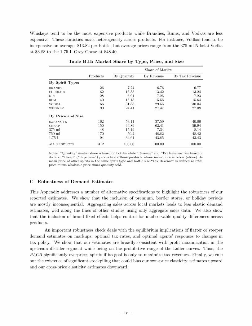
18Bacardi acquired Grey Goose from Sidney Frank in August 2004. Since PLCB requires a five-month advancenotice for any temporary price reduction, we assume that Sidney Frank manages the brand in our estimation andcounterfactuals. Table B.II in Appendix B reports the market shares by spirit type, bottle size, and price range.

– 16 –

While the overall market appears competitive with a Herfindahl-Hirschman Index (HHI)

based on bottle sales of only 930.3, distillers may have more market power within some regions

of the product space than others. For example, the HHI is approximately 3,000 for rums, while

the brandy and gin segments are moderately concentrated with HHIs of approximately 2,000.

The cordial, vodka, and whiskey segments have low concentration measures (all less than 1,400)

suggesting these segments are the most competitive. Horizontal differentiation of products within

a spirit class would provide further market power. An accurate characterization of the response

of distillers to changes in government tax policy therefore requires estimation of rich substitution

patterns underlying demand that motivates the observed extent of differentiation across and within

these different product segments.

3.4 Evidence of Heterogeneity of Preferences for Liquor

To conclude the description of the primary data features, we now document systematic variation

in consumer preferences along different demographic profiles. Throughout the analyses, we rely on

four primary demographic attributes of stores’ market areas: income, educational attainment, and

the prevalence of minority and young consumers. We used categorical data on income by minority

status to fit generalized beta distributions, which allow us to draw random samples of income for

our estimation from market-specific continuous distributions that vary by demographic trait and to

estimate the share of high-income households with incomes above $50,000. We similarly obtained

information on educational attainment by minority status to derive the share of the minority

and white population with at least some college education in each area. Lastly, we employ the

unconditional share of each market’s population between the ages of 21 and 29.

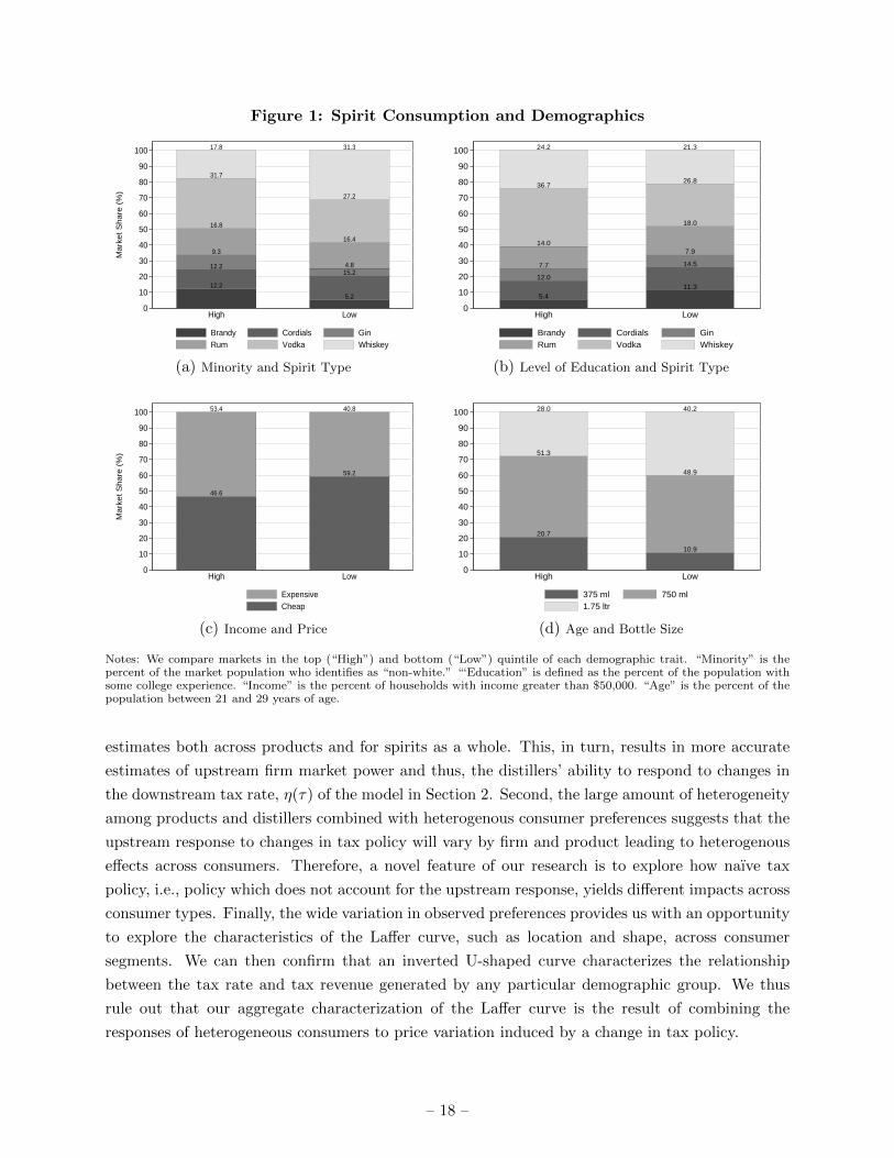
We show differences in preferences by assigning the store markets into quintiles based on

each demographic trait – the share of high-income households, the share of non-white or minority

households, the share of residents with some college education, and the share of residents in their

twenties. Figure 1 compares the purchase patterns of the top and bottom quintiles. Markets

with a greater share of minorities have substantially higher sales of vodka, gin, and brandy but

lower sales of whiskey. In areas where the population has more residents with college experience,

however, not only vodka but also whiskey is more popular, while rum and brandy have lower sales.

In markets with a larger share of high income residents, we observe larger purchases of expensive

spirits indicating that high income consumers are more willing to buy expensive spirits, presumably

because these spirits tend to be of higher quality.19 Finally, as the share of young residents increases,

so do sales of smaller bottles.

In our analysis, we exploit this wide variation in observable preferences across demographic

groups in three ways. First, this preference heterogeneity allows us to capture rich substitution

patterns to best reflect the purchase decisions of consumers, leading to more robust elasticity

19Our Proof66.com indicators confirm that price and quality are positively correlated, particularly for cordials, gins,and whiskeys.

– 17 –

Figure 1: Spirit Consumption and Demographics

12.2

12.2

9.3

16.8

31.7

17.8

5.2

15.24.8

16.4

27.2

31.3

0

10

20

30

40

50

60

70

80

90

100

Ma

rke

t S

ha

re (

%)

High Low

Minority

Brandy Cordials GinRum Vodka Whiskey

(a) Minority and Spirit Type

5.4

12.0

7.7

14.0

36.7

24.2

11.3

14.5

7.9

18.0

26.8

21.3

0

10

20

30

40

50

60

70

80

90

100

Mar

ket S

hare

(%

)

High Low

College

Brandy Cordials GinRum Vodka Whiskey

(b) Level of Education and Spirit Type

46.6

53.4

59.2

40.8

0

10

20

30

40

50

60

70

80

90

100

Ma

rke

t S

ha

re (

%)

High Low

Income

ExpensiveCheap

(c) Income and Price

20.7

51.3

28.0

10.9

48.9

40.2

0

10

20

30

40

50

60

70

80

90

100

Mar

ket S

hare

(%

)

High Low

Young

375 ml 750 ml1.75 ltr

(d) Age and Bottle Size

Notes: We compare markets in the top (“High”) and bottom (“Low”) quintile of each demographic trait. “Minority” is thepercent of the market population who identifies as “non-white.” “‘Education” is defined as the percent of the population withsome college experience. “Income” is the percent of households with income greater than $50,000. “Age” is the percent of thepopulation between 21 and 29 years of age.

estimates both across products and for spirits as a whole. This, in turn, results in more accurate

estimates of upstream firm market power and thus, the distillers’ ability to respond to changes in

the downstream tax rate, η(τ) of the model in Section 2. Second, the large amount of heterogeneity

among products and distillers combined with heterogenous consumer preferences suggests that the

upstream response to changes in tax policy will vary by firm and product leading to heterogenous

effects across consumers. Therefore, a novel feature of our research is to explore how naıve tax

policy, i.e., policy which does not account for the upstream response, yields different impacts across

consumer types. Finally, the wide variation in observed preferences provides us with an opportunity

to explore the characteristics of the Laffer curve, such as location and shape, across consumer

segments. We can then confirm that an inverted U-shaped curve characterizes the relationship

between the tax rate and tax revenue generated by any particular demographic group. We thus

rule out that our aggregate characterization of the Laffer curve is the result of combining the

responses of heterogeneous consumers to price variation induced by a change in tax policy.

– 18 –

4 Empirical Model

In this section we describe a static model of oligopoly price competition with differentiated goods.

We assume that each period upstream spirit manufacturers simultaneously choose wholesale prices

{pw} to maximize profits. The downstream firm, the PLCB , takes these prices as given and gener-

ates the final retail price by applying a 30% markup, a per-unit handling fee that varies by bottle

size, and an 18% liquor tax. Finally, consumers in each market choose the product that maximizes

their utility. We solve the model backwards, first presenting downstream consumer demand and

then progressing to the profit-maximization problem of the upstream spirit manufacturers.

4.1 Downstream Market - A Discrete Choice Model of Demand for Spirits

In modeling demand for spirits as a function of product characteristics and prices, we follow the

large literature on discrete-choice demand system estimation using aggregate market share data

(cf. Berry (1994), Berry, Levinsohn and Pakes (1995) (BLP), and Nevo (2001)). This facilitates

the estimation of robust own and cross-price elasticities for a large set of products while accounting

for systematic differences in consumer preferences across demographics.

In pricing period t, consumer i in market l obtains the indirect utility from consuming a

bottle of spirit j ∈ Jlt given by

uijlt = xjβ∗i + α∗i p

rjt + [ht q3t]γ + ξjlt + εijlt ,

where i = 1, . . . ,Mlt; j = 1, . . . , Jlt; l = 1, . . . , L; t = 1, . . . , T .(17)

The n× 1 vector of observed product characteristics xj is identical in all markets l where product

j is available and fixed over time, though the availability of different spirits may change over

time due to product introductions/removals or store closings/openings. We also include a holiday

dummy variable ht that indicates whether period t coincides with the end-of-year holiday season

from Thanksgiving to the New Year and a summer dummy variable q3t for the July, August, and

September periods. We denote the retail price of product j at time t by prjt where, in accordance

with the PLCB ’s pricing mandate, the retail price does not vary across markets l within period t.

We further allow utility to vary across products, markets, and time via the time and location-specific

product valuations ξjlt, which are common knowledge to consumers, upstream firms, and the PLCB

but unobserved by the econometrician.

We characterize consumer i in market l by a d-vector of observed demographic attributes

including education, race, youth, and income, that we denote by Dil. To allow for individual hetero-

geneity in purchase behavior, we model the distribution of consumer preferences over characteristics

and prices as multivariate normal with a mean νil that shifts with these consumer attributes,(α∗iβ∗i

)=

(α

β

)+ ΠDil + Σνil , νil ∼ N(0, In+1) , (18)

– 19 –

where Π is a (n + 1) × d matrix of coefficients that measures the effect of observable individual

attributes on the consumer valuation of spirit characteristics, while Σ measures the covariance in

unobserved preferences across characteristics. We restrict Σjk = 0 ∀k 6= j, and estimate only the

variance in unobserved preferences for characteristics. Introducing unobserved preferences for a

given characteristic j allows higher cross-price elasticities among products with similar characteris-

tics, e.g., flavored or imported, thereby relaxing the restrictive substitution patterns generated by

the Independence of Irrelevant Alternatives (IIA) property of the multinomial logit model. Simi-

larly, matrix Π captures the contribution of demographic and product characteristic interactions

that allows cross-price elasticities to vary differentially in markets with observed differences in

demographics. For instance, we expect expensive vodkas to have higher cross-price elasticities in

markets with a large fraction of high-income consumers.

Next, we follow Grigolon and Verboven (2014) in modeling the unobserved individual pref-

erences and assume that they are correlated across spirits of the same type, resulting in the random

coefficient nested logit model or RCNL. The term εijlt follows the distributional assumptions of

the nested logit model, thereby increasing the valuations of products within the same group (nest),

here given by spirit type. There are g = 0, 1, ..., G distinct groups to whom we assign each product;

we define group zero to be the outside good. We can therefore write the idiosyncratic valuation by

consumer i for product j in market l and period t as

εijlt = ζigt + (1− ρ)εijlt , (19)

where ρ ∈ [0, 1] and we assume that the distribution of ε is i.i.d. multivariate type I extreme value

and the distribution of ζigt is such that εijlt is also distributed extreme value. We define groups

according to spirit type (brandy, cordials, gin, rum, vodka, and whiskey), and call ρ the “nesting

parameter” as its value modulates the importance of spirit type in explaining consumer purchases.

As ρ goes to one, consumers view products within each spirit type as perfect substitutes while ρ

converging to zero reduces within-type correlation to zero. Plugging (19) into (17) yields

uijlt = xjβ∗i + α∗i p

rjt + [ht q3t]γ + ξjlt +

G∑g=1

1(j ∈ g)ζigt + (1− ρ)εijlt , (20)

where 1(j ∈ g) is a group indicator variable equal to one when product j belongs to spirit type

g. Together, equations (18) and (20) encompass several demand specifications allowing for a wide

arrange of substitution patterns. When Σ = 0 and ρ > 0 the model collapses to the nested logit.

Alternatively, when ρ = 0 but Σ > 0 the model collapses to the random coefficients model of BLP .

When both Σ = 0 and ρ = 0 the model returns the simple multinomial logit choice probabilities.

We assume that during a particular time period, each consumer selects either one bottle of

the Jlt spirits available in her market l or opts to purchase the outside option denoted by j = 0. We

– 20 –

define the potential market, Mlt, as all off-premise purchases, i.e., those purchases not consumed

in a restaurant or bar, of alcoholic beverages, including spirits, beer, and wine.20

The annual potential market for location l then is the number of drinking-age residents

scaled by per-capita off-premise consumption, which we calculate as follows. According to Haugh-

wout, Lavallee and Castle (2015) the average drinking-age Pennsylvanian consumed 124.2, 120.5,

and 121.0 liters of alcoholic beverages in 2002, 2003, and 2004, respectively. Of this consumption,

79.8% on average was purchased off-premise, resulting in per-capita off-premise consumption of

132.1, 128.3, and 128.7 bottle-equivalents of 750 ml, respectively.21 To put these figures in

perspective, beer accounts for approximately 90% of total consumption by volume so the average

drinking-age Pennsylvanian consumes the equivalent of nearly five 375 ml bottles of beer per week

vs. approximately four 750 ml bottles of both wine and liquor during the year.

The potential market Mlt for location l in period t is simply the prorated potential con-

sumption according to the number of days included in pricing period t. A consumer opting for

the outside option then consumes a 750 ml “bottle” of beer (i.e., two 375 ml bottles) or a 750

ml bottle of wine. Note that this definition of the potential market accounts for the total volume

of alcoholic beverages but not for the different ethanol contents of beer (4.5% on average), wine

(12.9% on average), and spirits (37.9% on average in our sample). Thus, policy can reduce total

ethanol consumption by increasing retail prices of spirits leading consumers to substitute towards

beer and wine.

Next, we address consumers’ choice decisions. The set of individual-specific characteristics

leading to the optimal choice of spirit j is given by

Ajt (pr·t, x·, ξ·t; θ) = {(Dil, νil, ε·lt) |uijlt ≥ uiklt ∀k = 0, 1, . . . , Jlt} , (21)

where we summarize all model parameters by θ. We follow the literature in decomposing the

deterministic portion of the consumer’s indirect utility into a common part shared across consumers,

δjlt, and an idiosyncratic component, µijlt. These mean utilities of choosing product j and the

idiosyncratic deviations around them are written as follows:

δjlt = xjβ + αprjt + [ht q3t]γ + ξjlt , (22a)

µijlt =(xj prjt

)(ΠDil + Σνil) . (22b)

In estimating the model, we take advantage of the additive specification of normally-

distributed deviations from mean utility and extreme-value random shocks to integrate over the

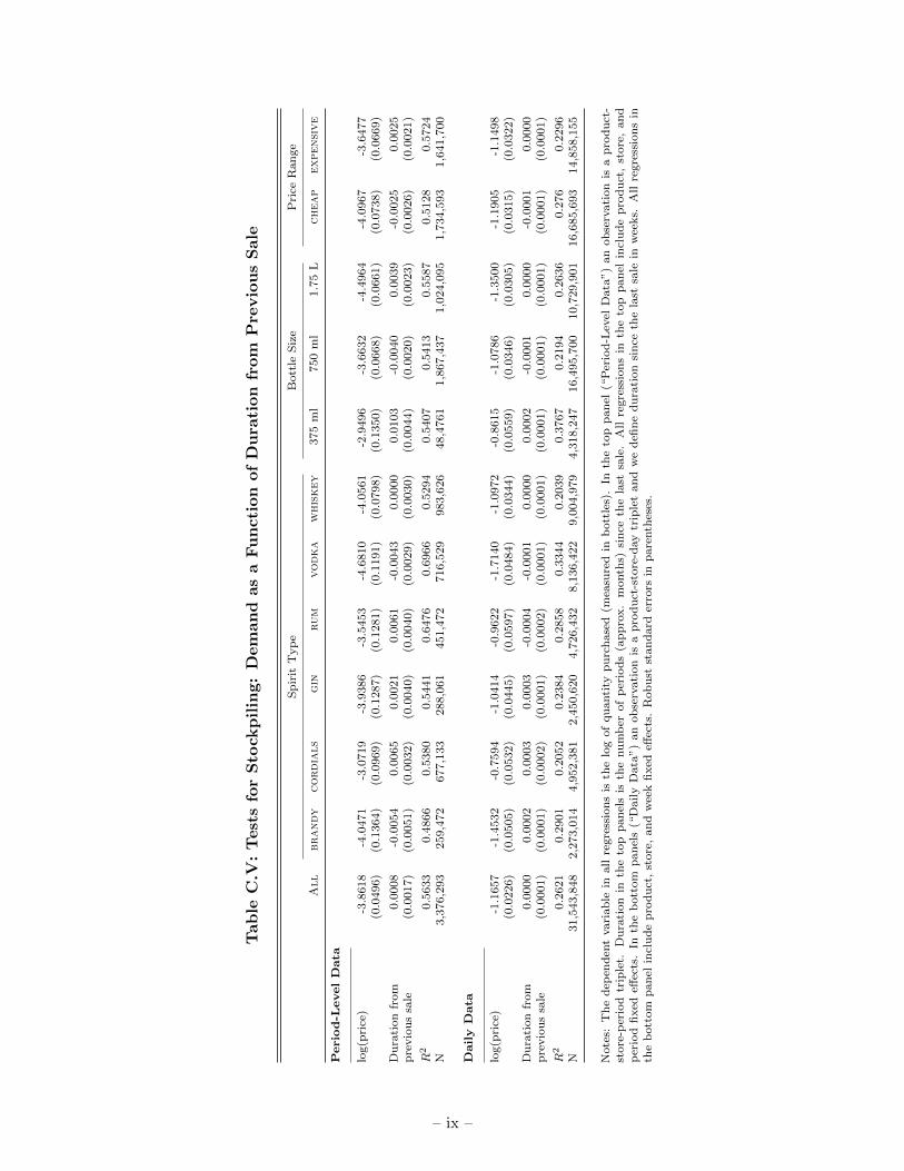
20The present static discrete choice approach has limitations when instead, individuals purchase several productsor multiple bottles of the same product at the same time. See Nevo (2000, p.401) and Hendel (1999). Hendeland Nevo (2006a) further show that static demand estimates overestimate own-price elasticities and underestimatecross-price elasticities when consumers make dynamic purchase decisions. We discuss potential issues and biasesassociated with stockpiling in Appendix C.4 as well as provide evidence that stockpiling is not an issue in our data.

21Authors’ calculations based on data from the National Alcohol Beverage Control Association.

– 21 –

distribution of εit giving rise to Ajt analytically. The probability that consumer i purchases product

j in market l in period t is then

sijlt =

exp

(δjlt + µijlt

1− ρ

)exp

(Iiglt

1− ρ

) ×exp(Iiglt)

exp(Iilt), (23)

where

Iiglt = (1− ρ) ln

Jg∑m=1

exp

(δmlt + µimlt

1− ρ

), (24a)

Iilt = ln

1 +G∑g=1

exp(Iiglt)

. (24b)

Deriving product j’s aggregate market share in each location requires integrating over the

distributions of observable and unobservable consumer attributes Dil and νil, which we denote by

PD(Di) and Pν(νi), respectively. Thus, the model predicts a market share for product j in market

l at time t of

sjlt =

∫νl

∫Dl

sijltdPD(Di)dPν(νi) , (25)

which we evaluate by Monte Carlo simulation. For each market l we simulate the consumption

choices of 200 randomly drawn heterogeneous consumers who vary in their demographics and

income. We construct the sample for each market using the previously discussed census data

on race, age, educational attainment, and income. We simulate whether each randomly drawn

consumer is a minority or in their twenties based on the prevalence of these demographic groups

in each market. Conditional on the consumer’s realized minority status, we then take a random

draw from the corresponding estimated continuous distribution of income and discrete distribution

of educational attainment. See Appendix A for further details. Since the ambient population

of stores changes with store openings and closings over the course of the sample, we allow the

simulated set of agents to also change. Lastly, we account for the unobserved preferences (ν) via

Halton draws in order to reduce simulation bias as recommended by Judd and Skrainka (2011).

4.2 An Oligopoly Model for Upstream Distillers

Wholesale prices pw are the outcome of an upstream market equilibrium given the PLCB ’s pricing

rule. We now present a flexible model of upstream behavior that places few restrictions on firm

conduct while allowing for robust estimates of upstream market power. Each firm f ∈ F produces

a subset Jft of the j = 1, . . . , Jt products and faces several competitors from the set F of upstream

distillers. In each period t the upstream firms simultaneously choose the vector of wholesale prices

{pwjt}j∈Jft to maximize period t profit

– 22 –

max{pwjt}

∑j∈Jft

(pwjt − cjt)×L∑l=1

Mltsjlt(pr(pw), x, ξ; θ

)︸ ︷︷ ︸

statewide demand forproduct j in period t

, (26)

where Mlt is the size of market l and cjt denotes the marginal cost of producing spirit j in period t.

Given the static nature of the firms’ pricing decisions, we omit the period t subscripts for the sake

of clarity going forward.22 Define as sj(pr, x, ξ; θ) =

∑Ll=1Mlsjl(p

r, x, ξ; θ) the state-wide demand

for product j. Assuming a pure strategy Bertrand-Nash equilibrium in wholesale prices, profit

maximization in the upstream market implies that upstream firm f chooses prices pwj ∀j ∈ Jf to

solve the set of first-order conditions

sj(pr(pw), x, ξ; θ

)+∑m∈Jf

(pwm − cm)sm(pr(pw), x, ξ; θ

)× ∂sm∂pwj

= 0 . (27)

The term ∂sm∂pwj

is the change in quantity sold for product m in response to a change in the wholesale

price and, through the pricing rule, the retail price of product j.23 Converting (27) into vector

notation yields

pw = c+ [Ow ∗∆w]−1 × s(pr(pw), x, ξ; θ)︸ ︷︷ ︸vector of wholesale markups

, (28)

where Owt denotes the ownership matrix for the upstream firms with element (j,m) equal to one

if goods j and m are in Jf . We define ∆w as a matrix that captures changes in demand due to

changes in wholesale price as follows

∆w=∆d∆p′=

∂s1∂pr1

. . . ∂s1∂prJ

.... . .

...∂sJ∂pr1

. . . ∂sJ∂prJ

dpr1dpw1

. . .dpr1dpwJ

.... . .

...dprJdpw1

. . .dprJdpwJ

′

=

∂s1∂pr1

. . . ∂s1∂prJ

.... . .

...∂sJ∂pr1

. . . ∂sJ∂prJ

1.534 . . . 0...

. . ....

0 . . . 1.534

, (29)

where ∆d is the matrix of changes in quantity sold in period t due to changes in retail price with

element (r,m) equal to ∂sr∂prm

and ∆p is the matrix of changes in retail price due to changes in

wholesale price with element (m, j) equal to dprmdpwj

.

22Table II documents that the PLCB limits the number of times distillers can temporarily reduce a product’s price.In the data, the average product goes on sale only 2.3 times per year and 76.6% of products go on sale three timesor less in a year, indicating that this regulation does not constrain upstream pricing for the majority of products.We thus do not address any dynamic considerations to the timing of pricing decisions over the course of the year,but employ a simpler and more tractable static pricing model instead.

23For simplicity, we assume that firms observe the distribution of consumer preferences. We thus abstract fromsecond-degree price discrimination across bottle sizes as in in McManus (2007) and instead focus on horizontaldifferentiation between products.

– 23 –

Villas-Boas (2007) shows that in vertical retail pricing markets, ∆p can be a complicated

object. In our context, however, the state’s regulation of alcohol sales simplifies this matrix

significantly by committing downstream stores to a uniform pricing policy and by eliminating

off-diagonal terms. For example, under the current pricing rule,dprjdpwj

is simply 1.30×1.18, reflecting

the 30% uniform tax and the 18% liquor tax that translate a change in the wholesale price for

product j to a change in the product’s retail price. Further, the retail price for product m does

not respond to a change in the wholesale price for product j: dprmdpwj

= 0 ∀m 6= j. The uniform tax

rule from equation (16) thus limits the PLCB ’s ability to respond to changes in wholesale prices

chosen by the upstream firms, resulting in a diagonal price response matrix ∆p.

We rely on this model of firm behavior in the following ways. First, we use the firms’

first-order necessary conditions for profit-maximization in equation (28) to back out product-level

marginal costs given demand estimates and observed wholesale and retail prices. This enables us to

measure wholesale markups and thus the degree of market power in the upstream market. Second,

we use equation (28) to evaluate the optimal distiller response to changes in PLCB tax policy,

which we denote as η above. Third, the upstream model allows us to consider alternative forms of

upstream conduct, by varying the definition of the ownership matrix Ow. We exploit this flexibility

to explore how different conduct assumptions impact upstream market power, our estimates of the

upstream response to taxes η, and ultimately the shape and location of the Laffer curve.

5 Identification, Estimation, and Demand Model Results

In this section we outline an estimation approach similar to Nevo (2000) but adapted to the

institutional features surrounding the price regulation of spirits in Pennsylvania. We present a

three-step estimation procedure that takes advantage of the fact that distillers set a single wholesale

price that the PLCB translates into a single retail price across all local markets. This allows

us to identify the contribution to demand of unobserved Σ and observed Π demographic taste

heterogeneity across the state at a point-in-time and the nesting parameter ρ defined over spirit

type separately from the contribution of common, but time varying, shifters of each product’s mean

utility (α, β). In identifying the price coefficient α we discuss potential sources of price endogeneity,

which in our case stem from the response of distillers to downstream consumer demand shocks

rather than from the PLCB ’s pricing behavior. We then present the model estimates and discuss

the implied demand elasticities ε(pr) and upstream response elasticities η(τ).

5.1 Estimating the Random Coefficients and Demographic Interactions

We begin with a description of the first of the three stages of our estimation procedure where

we estimate the contributions of product characteristics Σ and demographic interactions Π to the

deviations from mean utility, µijlt, controlling for location and product by time fixed effects and

the spirit type via ρ. We follow the earlier literature in using a generalized method of moments

– 24 –

estimator, GMM , that interacts a structural demand side error ω(Σ,Π, ρ) with instruments Z. To

define ω, we decompose the unobserved product valuations, ξjlt, as follows:

ξjlt = ζ1l + ξjt + ∆ξjlt . (30)

In equation (30), ζ1l is a location fixed effect that captures systematic variation across

markets in the preference for spirits consumption relative to beer and wine. This also accounts for

the fact that while per-capita consumption of alcoholic beverages likely varies across Pennsylvania,

such disaggregated data is not available and we define the potential market to be the average

Pennsylvanian’s consumption of off-premise alcoholic beverages. We control for systematic variation

in preferences for a given product over time via ξjt, to reflect the fact that across the state, a

product’s mean demand varies over the course of the year. With this specification, the mean utility

of product j, δjlt in equation (22a), simplifies to

δjlt = ζ1l + ζ2

jt + ∆ξjlt , (31)

where the product and time specific fixed effect ζ2jt subsumes the effect of product characteristics,

seasonal buying, and price on a product’s mean utility.

Equation (31) highlights an advantage to our setting: since price does not vary across

locations l, we are able to control for its mean contribution to utility via product by time fixed

effects, which we then use in a second stage estimation to isolate α. The remaining structural error

ω therefore represents deviations in unobserved product valuations within a store, ∆ξjlt, from these

mean product-time valuations after controlling for the average taste for spirits in market l.

We define our parameters of interest in this estimation stage as θA = {Σ,Π, ρ}, and we solve

for the structural error ω(θA) = ∆ξjlt using the following algorithm. For a given guess at θA, we

find the mean-utility levels δjlt(ζ1l , ζ

2jt, Sjlt; θA) that set the predicted market share of each product,

sjlt in equation (25), equal to the market share observed in the data, Sjlt.24 We follow Somaini

and Wolak (2015) and use a within transformation of δ to remove the store and product-period

fixed effects ζ1l and ζ2

jt, leaving only ω. Define Z+ as the within transformation of the instruments

matrix Z; e.g., for instrument k, Z+,kjlt = Zkjlt − Zkjt − Zkl . The GMM estimator exploits the fact

that at the true value of the parameters (Σ?,Π?, ρ?), the instruments Z+ are orthogonal to the

structural errors ω(Σ?,Π?, ρ?), i.e., E[Z+′ω(θ?)

]= 0, so that the GMM estimates solve

θA = argminθA

{ω(θA)′Z+W+Z+′ω(θA)

}, (32)

where W+ is the weighting matrix, representing a consistent estimate of E[Z+′ωω′Z+]. Finding

a global solution to a highly nonlinear problem such as this is difficult and any line, gradient, or

24We rely on the contraction mapping outlined in Appendix I of BLP . In order to ensure convergence to consistentstable estimates we follow the advice of Dube, Fox and Su (2012, §4.2) and set the norm for the mean valuecontraction equal to 1e-14.

– 25 –

simplex search would likely only result in a local solution. To increase the likelihood of achieving a

global minimum, we employ the Knitro Interior/ Direct algorithm suggested by Dube et al. (2012)

starting from several different initial conditions to ensure robustness of our results.25

5.1.1 Identification of Random Coefficients and Demographic Interactions

Identification of Σ and ρ comes from correlation between a product’s market share and its character-

istics relative to other more or less similar products – see Berry and Haile (2014). We construct two

instruments similar to those used in Bresnahan, Stern and Trajtenberg (1997). First, we employ the

number of products in the market that share product j’s characteristic. For example, to identify a

random coefficient for imported varieties, we use the total number of competing imported products

of the same bottle size in market l as the instrument for a given imported product. To identify the

nesting parameter, ρ, we use the total number of competing products of the same spirit type in

market l, separately for each spirit type. Second, we use spirit product scores from Proof66.com as

a measure of product quality and compute the average distance, measured in squared deviations,

of product j to other products that share its characteristic. Thus, for the above imported product,

this would be the average distance in product score space from other imported products in location

l. This instrument provides additional identifying power since it allows for differential effects

of introducing a high-quality imported product into a market with other high-quality imported

products versus into a market populated by largely low-quality imported products.26

We base identification of Π on correlation between a product’s market share in a given store

market and the demographics of the population served by each store. We thus interact the above

instruments with the prevalence of a given demographic attribute in each market. For example, we

identify the differential taste of young households for vodkas by interacting our earlier instruments

for vodka with the share of young consumers in each market. In the case of the interaction of

income with price, we construct the first instruments based on the product’s price category (cheap

vs. expensive) and interact them with the share of households in the market with income about

$50,000. Berry and Haile (2010) point out that these instruments proposed by Waldfogel (2003)

are valid provided there exist no demand spillovers from consumers in other similar markets.

5.2 Estimating Mean Utility Coefficients

In the second and third stages of estimation, we estimate mean utility coefficients given the

estimated first-stage coefficients θA and the resulting product-by-time fixed effects ζ2jt(θA). We

project ζ2jt onto price and the seasonal indicators, controlling for product fixed effects ζj ,

25 In constructing our optimal weighting matrix, we first assume homoscedastic errors and use W+ = [Z+′Z+]−1

to derive initial parameter estimates. Given these estimates, we solve for the structural error ω and constructE[Z+′

ωω′Z+]−1 as a consistent estimate for W+.26For example, the introduction of a high-quality Scotch whiskey into a location can therefore have differential effects

on the market shares of other Scotch whiskeys and the market shares of lower-quality Canadian whiskeys.

– 26 –

ζ2jt = [ht q3t]γ + αpjt + ζj + ξjt . (33)

Equation (33) highlights the potential for price endogeneity, to the extent that price re-

sponds to time-varying preference variation for a given product that is common across locations,

in the form of, for example, seasonal variation in consumption. Since the PLCB ’s pricing rule

applies a fixed markup to wholesale price irrespective of local or seasonal demand responses, its

pricing cannot respond to such unobserved demand shocks. But the predictable link between

wholesale and retail prices opens the possibility to spirit prices being endogenous not because of

the pricing practices of the PLCB , but because of the pricing behavior of upstream distillers whose

chosen wholesale prices reflect, through market shares, the unobserved common tastes for product

characteristics of spirits, ξjt. Recall the pricing optimality conditions in equation (28).

In principle, the fact that distillers need to request both temporary and permanent changes

to their wholesale price a number of months before the new price takes effect mitigates such

endogeneity concerns. Prices thus only respond to predictable variation in a product’s demand

over time. At the same time, none of our product characteristics vary across time, limiting our

ability to flexibly represent such time varying preference heterogeneity at the level of the product.

We therefore use instrumental variables techniques to estimate the parameters in equation (33)

using two sets of instruments for price.

First, we rely on the contemporaneous average price of a given product from liquor control

states outside of the Northeast and Mid-Atlantic regions.27 Our identifying assumption is that

cost shocks are national, since products are often produced in a single facility, but demand shocks

are largely regional, linked to differences in climate and demographics, which correlate with con-

sumption as we establish in Section 3.4. We thus focus on product prices in control states that

are distant from Pennsylvania and have sufficiently different demographic profiles and climates

to support the assumption that their demand shocks are uncorrelated with Pennsylvania’s. For

example, states such as Idaho, North Carolina, Oregon, and Wyoming have at least a 50% higher

share of Hispanics than Pennsylvania’s low six percent, while only North Carolina has a significant

prevalence of African Americans (at 22% double Pennsylvania’s 11% share), but also a very different

climate. The latter is helpful since, e.g. whiskey consumption peaks during colder months and the

appeal of whiskey thus varies significantly between Pennsylvania and the states used to construct

the instrument. Given that most price changes in the data are temporary, rather than permanent,

a concern with this instrument would be possible coordination of sales across the control states.

We find little evidence of such coordination, however.28

27An “alcohol control state” is a state that has monopoly over the wholesale or retail sales of some or all categoriesof alcoholic beverages. As of 2016, this list includes: Alabama, Idaho, Iowa, Maine, Maryland (Montgomery,Somerset, and Wicomico counties), Michigan, Mississippi, Montana, New Hampshire, North Carolina, Ohio,Oregon, Pennsylvania, Utah, Vermont, Virginia, West Virginia, and Wyoming. Washington state privatized itsalcohol retail distribution in 2012.

28We define a price reduction in our price instruments as “temporary” when price falls for one month. We then testwhether these indicators are correlated with temporary price reductions in Pennsylvania using Kendall’s τ , which

– 27 –

Figure 2: Changes in 2003 Retail Price ($)

10

12

14

16

18

20

22

24

26

28

Mar May Aug Sep Dec

Bacardi Limon - 750 ml ($12.79)

Bacardi Limon - 1.75 ltr ($25.70)

Beefeater - 750 ml($18.03)

Jameson Irish Whiskey - 750 ml($22.67)

Shelf Price Across Time(Select Products)

We add to this instrument changes in input prices, sugar and corn, interacted with spirit type

indicators to account for exogenous cost shifts across spirit types, e.g., a major input for cordials

and rums is sugar, while corn is an input to gins, vodkas, and whiskeys. Including input price

interactions for barley, glass, oats, rice, rye, sorghum, and wheat did not improve the estimates; we

therefore do not use them in our primary specification.

Next we collapse the second stage parameters into vector θB as follows

θB = (XB′XB)−1XB

′ζ2 (34)

where XB = ZB(Z ′BZB)−1Z ′BXB, XB = [ht q3t pjt ζj ], and ZB is the matrix of price instru-

ments. In the third and final estimation step, we recover product fixed effects ζj from equation (34)

and project the vector ζ onto the matrix of observable product characteristics x, resulting in:

θC = (x′x)−1x′ζ . (35)

Variation in prices over time identifies the price coefficient, exploiting the fact that distillers

do not change the wholesale prices pw for all products at the same time. This introduces variation in

relative prices depicted in Figure 2. We identify seasonality and mean preferences for time-invariant

product characteristics such as proof and spirit type from systematic variation in market shares of

spirits by time period or characteristic.

we find to be low (on average 0.03 across state-pairs). This indicates that these temporary price changes do notappear to be correlated.

– 28 –

5.3 Estimation Results

Table IV presents the demand estimates of our preferred specification of the RCNL model using the

three-step procedure outlined above. Parameters are very precisely estimated. Estimated demand

for spirits increases during the summer and the holiday season. On average, consumer valuations

of brandy, cordials, and whiskey exceed gin (our reference category), while rums and vodkas are,

on average, less valued. Consumers prefer 1.75 L to smaller bottles driven by the fact that when a

Table IV: RCNL Demand Estimates

Mean Utility Random Coeff. Demographic Interactions (Π)

(β) (Σ) Income Young Minority College

price -0.3062 0.1151(0.0036) (0.0036)

holiday 0.3153(0.0057)

summer 0.0557(0.0049)

375 ml -2.9554(0.5608)

750 ml -7.5816 0.5939 22.7684 0.4025 4.9886(0.4037) (0.3061) (3.2953) (0.0844) (0.2976)

brandy 0.3882 0.8616 1.3978 -0.8738(0.6902) (0.2288) (0.0231) (0.0518)

cordials 0.2977(0.7163)

rum -4.7646 11.5406 -0.1628 0.6795(0.8355) (2.9485) (0.0146) (0.0426)

vodka -1.9611 4.9747 -0.3713 4.2314(0.4835) (0.6656) (0.0233) (0.2701)

whiskey 0.3875 1.2203 -0.9270 0.9549(0.5123) (0.2059) (0.0231) (0.0554)

flavored 3.7007 -4.9731 -0.5111 -3.2395(0.4848) (0.7219) (0.0374) (0.1943)

imported 1.3598 0.1912(0.3519) (0.5134)

proof 15.1897 1.2575 -26.0064 1.6695 -5.5765(1.6844) (0.2505) (4.2377) (0.0913) (0.4402)

quality 3.9347(2.1101)

constant -15.3884(1.8244)

Nest (ρ) 0.1225(0.0139)

Notes: Robust standard errors are reported in parentheses. Estimates for random coefficients Σ,demographic interactions Π, and nesting parameter ρ based on GMM estimation using 3,377,659observations in 12,957 markets given by store-period pairs and 200 simulated agents in each market.Mean utility estimates for price, holiday, and summer are based on the projection of estimated product-period fixed from the GMM estimation onto corresponding characteristics plus product fixed effectsafter controlling for price endogeneity. Remaining mean utility estimates based on the projection ofestimated product fixed effects onto the remaining observable product characteristics.

– 29 –

brand is available in several bottle sizes, the 1.75 L is more popular, all else equal. Consumers also

prefer imported, flavored, and high proof products.

These are only average valuations. We also allow for rich variation across demographics

by interacting the young, minority, and college-educated indicators with spirit type, bottle size,

and proof. The estimates of Π reveal significant differences in tastes for spirits across demographic

groups. We find that demand becomes steeper as consumers become wealthier, consistent with

the increased consumption of expensive spirits by “high income” consumers presented in Figure 1.

Consumers of different demographic groups often do not favor the same spirits: Although the

average consumer values vodkas less than gins, individuals with some college education strongly

favor them. These consumers also dislike brandy but favor whiskeys, while minorities rank brandy

over gin and then whiskey. Young consumers have a marked preference for rum and 750 ml bottles.

Despite the large number of demographic interactions included in Π, we still find statistically

significant values for the random coefficients (Σ) for proof and 750 ml bottles. We also obtain a

significant estimate of the spirit type nesting parameter ρ, indicating that although products within

a spirit type are far from being perfect substitutes to each other, they are better substitutes than

those of a different spirit category. Figure 3 corroborates this point. In the figure we present the

ratio of the average cross-price elasticity between each product and products of its own spirit type

(e.g., rums) to that between the product and all other products (brandies, cordials, gins, vodkas,

and whiskeys). The results indicate the demand estimates generate sensible cross-price elasticities

where the best substitute for a Captain Morgan is another rum, say a Bacardi.29

Figure 3: Cross-Price Elasticities by Type

17.1

6.5

18.1

9.8

7.4

5.8

0

2

4

6

8

10

12

14

16

18

20

Avg

. Cro

ss-P

rice

Ela

stic

ity (

In)

/ Avg

. Cro

ss-P

rice

Ela

stic

ity (

Out

)

BRANDY CORDIALS GIN RUM VODKA WHISKEY

29 In Table D.I in Appendix D we document the best estimated substitutes for a variety of popular products.

– 30 –

Table V: Price Endogeneity

OLS IV1 IV2 IV3 IV4

price -0.2673 -0.3062 -0.3073 -0.3114 -0.3128(0.0027) (0.0036) (0.0036) (0.0037) (0.0037)

First-Stage F-Stat.: — 1,333.19 1,297.06 1,217.18 1,196.74

Instruments:- Input Prices X X X X- Alabama X- Iowa X X- Idaho X X X X- Michigan X- Mississippi X- Montana X X X- North Carolina X X- Oregon X X X X- Utah X- Wyoming X X X X

Notes: All estimates based on 10, 532 observations. Specifications include the same covariates asin Table IV. Price instruments based on the average contemporaneous price among alternative setsof control states outside the Northeast and Mid-Atlantic regions. “Input Prices” corresponds tocontemporaneous commodity prices for inputs (corn, sugar) interacted with spirit type to furtherseparate cost and demand shocks.

This comparison relies in part on our estimated price coefficient. As discussed above, we

use the contemporaneous average price in distant control states and commodity prices for corn and

sugar interacted with spirit type dummies as price instruments. In Table V, we document that our

estimate of the price coefficient is both sensible and robust. In particular, we compare the estimated

price coefficient using alternative two-stage least squares results of the estimated first stage product-

period fixed effects projected onto price, seasonal dummies, and product fixed effects. Relative

to IV1, our preferred specification, the estimated price coefficients are stable across alternative

instruments, and, as expected, entail larger price responses than a simple OLS specification. Each

estimated price coefficient is significant at the 95% level, each IV price coefficient is significantly

different than the OLS specification, and the set of IVs generates significant F-statistics for all

specifications.

Table VI presents descriptive statistics for product elasticities using the IV1 price coefficient.

Overall, our product elasticities are sensible and similar to Conlon and Rao (2015) and Aguirre-

gabiria et al. (2016) who estimate alcohol demand using disaggregate data. At the product-level,

we estimate an average own-price elasticity of −3.86 although there is substantial heterogeneity

in elasticities that correlates with spirit types and bottle sizes. Rums, brandies, and cordials tend

to be less elastic compared to vodka and whiskey products, though the empirical distribution of

estimated price elasticities is most spread for whiskeys and gin and most concentrated for rums.

The bottom of Table VI shows that the demand for 375 ml bottles is more inelastic than for the 1.75

L bottles, with the medium-sized 750 ml bottles in-between. We also find that expensive products

have more elastic demands than cheap spirits.

– 31 –

Table VI: Estimated Product Elasticities, Upstream Marginal Costs, and UpstreamMarket Power

ε(pr) c Lerner

Price Avg SD Avg SD Avg SD

By Spirit Type:

brandy 15.41 -3.65 1.49 5.92 4.49 37.56 17.00cordials 14.57 -3.64 1.22 5.78 3.74 35.26 12.23gin 15.15 -3.86 1.54 6.69 5.10 34.86 13.78rum 13.15 -3.57 1.08 5.36 2.97 36.66 12.86vodka 16.66 -4.05 1.47 7.11 4.77 34.67 18.73whiskey 16.65 -4.07 1.50 7.29 4.95 32.51 12.90

By Price and Size:

expensive 20.37 -4.73 1.37 9.43 4.62 25.94 8.15cheap 11.04 -3.04 0.84 3.79 1.98 42.92 14.75375 ml 9.16 -2.54 0.83 2.71 2.07 53.54 20.32750 ml 14.43 -3.76 1.23 5.99 3.57 34.35 11.281.75 L 21.16 -4.68 1.39 9.34 5.13 26.30 6.80

all products 15.63 -3.86 1.41 6.53 4.51 34.66 14.70

Notes: “Price” is measured in dollars; “Average” refers to the simple average of the corresponding category while “SD” is thestandard deviation. Appendix D presents the full elasticity distributions by spirit type and bottle size. Estimated marginalcosts (c) based on product-level marginal costs for each pricing period using the firm first-order conditions in equation (28)under the assumption that firms set prices for products in their observed product portfolios. “Lerner” is the average Lerner

index defined as 100× pw−cpw

.

In Table VII we demonstrate that our demand estimates translate into variation in the

estimated elasticities by consumer demographics. For each market we calculate average elasticities

across simulated consumers, and, as in Section 3.4, we compare markets in the top and bottom 20%

for each demographic trait. Markets with high concentrations of wealthy and educated consumers

exhibit product demands that are relatively less elastic, while markets with concentrations of young

people tend to have more elastic demands for spirits. Demand for spirits as a category is less elastic

in markets with large minority populations and markets with greater levels of income and education.

The model estimates imply an average price elasticity of off-premise spirit demand of −2.8.

That is, a one percent increase in the retail price of all spirits leads to a 2.8% decrease in the

aggregate quantity of off-premise spirits demanded. Earlier literature, however, documents less

elastic demand estimates for alcoholic beverages in general, and spirits in particular. Based on

a review of the literature, Leung and Phelps (1993) conclude that the price elasticity of demand

for distilled spirits is −1.5. Two effects likely drive the discrepancy between our results and this

work. First, rather than estimating the elasticity of total alcohol consumption, we exclude the

presumably less price sensitive consumption in bars and restaurants. Second, the earlier studies

use state or national consumption data whereas we have detailed local data on consumption choices.

In Appendix C.1 we show that aggregation in our data drives the price coefficient and consequently

the estimated elasticity for spirits towards zero. We also show in Table C.III that values of the

price coefficient that generate elasticities consistent with Leung and Phelps (1993) imply demand

curves which are inconsistent with upstream profit-maximization.

– 32 –

Table VII: Estimated Product Elasticities Across Demographics

Income Young Minority College

Low High Low High Low High Low High

Outside Good -2.98 -2.64 -2.74 -2.83 -3.06 -2.78 -3.07 -2.61

By Spirit Type:

brandy -4.01 -3.24 -3.40 -3.86 -3.61 -3.94 -3.87 -3.33cordials -4.06 -3.18 -3.43 -3.79 -3.80 -3.85 -4.00 -3.24gin -4.19 -3.48 -3.70 -3.94 -4.11 -3.93 -4.18 -3.50rum -3.96 -3.12 -3.36 -3.71 -3.72 -3.76 -3.91 -3.18vodka -4.42 -3.60 -3.84 -4.18 -4.18 -4.24 -4.38 -3.62whiskey -4.43 -3.64 -3.87 -4.21 -4.24 -4.26 -4.42 -3.68

By Price and Size:

expensive -5.17 -4.21 -2.85 -3.18 -4.94 -4.93 -5.15 -4.23cheap -3.39 -2.64 -4.49 -4.86 -3.18 -3.21 -3.34 -2.70375 ml -2.80 -2.22 -2.37 -2.68 -2.58 -2.70 -2.73 -2.29750 ml -4.18 -3.29 -3.53 -3.93 -3.89 -4.00 -4.12 -3.351.75 L -5.08 -4.21 -4.44 -4.83 -4.84 -4.90 -5.05 -4.25

all products -4.24 -3.43 -3.66 -4.00 -4.01 -4.05 -4.19 -3.47

Notes: Statistics are the simple average product elasticity in the relevant category-demographic pair. Demographic categoriesare defined in Section 3.4. “High” refers to markets in the top 20% while “Low” refers to markets in the bottom 20% for thecorresponding demographic trait.

5.4 The Upstream Marketplace

Of central interest for characterizing the Laffer curve in this industry are estimates of upstream

market power and therefore an estimate of the upstream response elasticities η. To be able to

simulate an upstream response to changes in the downstream tax rate, we require estimates of

distiller marginal cost. Using our demand estimates and the data on price and quantity sold

alongside the above model of distiller conduct of Section 4.2, we back out product-level marginal

costs for each pricing period using the firm first-order conditions in equation (28).30 In the absence

of allegations of collusion among distillers during the sample period, we assume that they compete in

setting wholesale prices by internalizing the effect of a change on a product’s price on the remaining

products in their portfolio. Thus, as in Section 4.2, the ownership matrix Ow simply reflects the

firms’ portfolios during the sample period.31

The cost estimates c that result from firm optimization under the observed wholesale prices

and estimated demand are reasonable (see middle columns of Table VI). The marginal cost of

expensive products is on average 2.5 times that of inexpensive products; for a subset of brandies

and whiskeys with detailed product information, we find that those products that are aged for five

or more years have marginal costs of 1.3 for brandies and 1.4 times for whiskeys that of non-aged

products. Lastly, imported products are 1.8 times more costly than non-imported products on

average.

30The fact we observe both wholesale and retail price data allows us not to impose any supply-side restrictions onprices during estimation which alleviates the identification concerns of Villas-Boas and Hellerstein (2006).

31A comparison of marginal cost estimates across a variety of conduct assumptions did not provide any clear evidencein favor a non-competitive equilibrium.

– 33 –

We use these cost estimates to assess market power in the upstream distillery market,

which we summarize in the last columns of Table VI. We find that upstream firms do indeed

have significant market power, enjoying an average Lerner index of 34.66%: For every one dollar

of product sold to the PLCB distillers take home 35 cents in profits. Diageo, Bacardi, and

Beam products generate average margins of 32.5%, 32.2%, and 38.1%, respectively.32 Small bottle

products have higher margins (54% on average) than large bottles (26% on average) due to their

substantially less elastic demand (third column of Table VI). There is less heterogeneity across

spirit types as the average whiskey generates a margin of 32.5% compared to 37.6% and 36.7% for

the average brandy and rum, respectively.

Table VIII: The Upstream Firm Response toChanges in Tax Policy

Wholesale Price ConsumerResponse (η) Pass-Through

Avg SD Avg SD

By Spirit Type:

brandy −0.20 0.12 0.41 0.12cordials −0.19 0.08 0.42 0.09gin −0.21 0.10 0.42 0.10rum −0.20 0.09 0.40 0.09vodka −0.18 0.12 0.43 0.12whiskey −0.17 0.09 0.44 0.10

By Price and Size:

expensive −0.13 0.06 0.49 0.06cheap −0.24 0.10 0.36 0.09375 ml −0.31 0.13 0.30 0.13750 ml −0.18 0.07 0.42 0.081.75 L −0.13 0.04 0.48 0.06

all products −0.19 0.10 0.42 0.10

Notes: “Avg” and “SD” are the simple average and standard deviation forproducts within the spirit type, bottle size, or price range. “Price Response”corresponds to the wholesale price response of the upstream firms defined asthe percent change in wholesale price given a one percent increase in the advalorem tax rate. “Consumer Pass-Through” is the percent change in retailprice from a one percent increase in the ad valorem tax rate. All statistics arecalculated at the estimated equilibrium assuming upstream conduct basedon product ownership.

These estimates of upstream market power suggest that upstream firms can do much to

counteract changes in PLCB policy. Table VIII shows that overall, a one percent increase in the

tax rate at the current equilibrium induces upstream firms to reduce wholesale price by 0.19% on

average. We see significant heterogeneity within and across product categories as the reduction in

wholesale price is greatest among cheap and 375 ml products, but varies little across spirit types.

32We test the validity of these estimates against the financial disclosures for seven public firms in our sample and findthat our estimates of the Lerner index compare favorably to these firms’ gross profit margins during the period.For instance, we estimate that firms earn 34.66 cents per dollar of revenue on average compared to an average grossprofit margin of 37.80% among public distillers. We also see a similar pattern across firms, e.g., Diageo’s grossprofit margin (30.04%) is lower than Beam’s (46.06%).

– 34 –

In terms of retail pass-through the upstream wholesale price response limits retail price increases to

0.42% on average, significantly less than the 1% tax increase that would have been added to prices

were firms pricing at marginal cost. In the remaining section we assess the quantitative significance

of upstream market power for correctly characterizing the Laffer curve and investigate how the

ability of distillers to re-optimize their wholesale pricing might undo the objective of the regulator.

6 Laffer Curves: Policymaker Foresight and Market Conduct

We now use our estimates of spirit demand and upstream marginal costs to assess distiller responses

to changes in the PLCB ’s tax policy and their effect on the revenue the PLCB earns from its pricing

policy. The goal of this section is thus to characterize the Laffer curve as the PLCB varies its ad

valorem tax, τ , while holding other aspects of the pricing regulation fixed. The ad valorem tax is

used by most control and non-control states in the regulation of alcohol. Throughout our analysis

we focus on the ability of the PLCB to generate tax revenue. In line with our focus on maximizing

tax revenue are ongoing efforts at reforming the Pennsylvania wine and spirits retail markets.

For example, the Pennsylvania Legislature’s Act 39, which took effect in August 2016, granted

the PLCB limited pricing flexibility in allowing it to price its best-selling items, defined as the

top-selling 150 SKUs, “in a manner that maximizes the return on the sale of those items.”33

We first characterize the Laffer curve by assuming the regulator is naıve and mistakenly

believes that upstream firms lack the interest or ability to react to changes in policy. In the

notation of the model of Section 2, η(τ) = 0. We then allow upstream firms to respond to changes

in policy under different assumptions regarding upstream conduct – multi-product, single-product,

or monopoly pricing – enabling us to characterize the effect of the degree of imperfect competition

on the location and shape of the Laffer curve not only in aggregate but also for different consumer

groups. Finally, we contrast the Naıve equilibrium with one where the regulator fully anticipates

distillers’ strategic responses to reveal the implications of assuming perfect competition among

firms. Our analysis shows that the location and shape of the Laffer curve fundamentally depend on

the degree to which the regulator rightly anticipates the response of distillers to changes in PLCB

policy. Moreover, abstracting from firm responses (i.e., the Naıve equilibrium) leads to policy

recommendations that not only miss aggregate objectives but also generate inequitable effects

across different consumers.

6.1 The Laffer Curve and Naıve Policymakers

A regulator and 37 firms producing 312 products may interact in multiple ways. The degree to

which the PLCB understands and internalizes the optimal responses of distillers and consumers

to changes in tax policy is unclear. Rather than taking a stand on the ability of the PLCB to

33Omnibus Amendment to Pennsylvania’s Liquor Code, Act of Jun. 8, 2016, P.L. 273, No. 39. Full text available athttp://www.legis.state.pa.us/cfdocs/legis/li/uconsCheck.cfm?yr=2016&sessInd=0&act=39. At the time ofthis writing, the PLCB has taken advantage of this pricing flexibility only a limited number of times.

– 35 –

anticipate agents’ responses, we choose to use the model to evaluate the influence of distillers on

the final outcome of the policy under different beliefs or information assumptions on the part of

the regulator.

6.1.1 Mechanical Effect

The first alternative we consider is an application of the famous critique of Lucas (1976) in which the

PLCB naıvely believes distiller behavior is invariant to its policy. This is the so-called “mechanical

effect” of taxation where we assume firms do not respond to changes in the tax policy though

we do allow for re-optimization of consumers to changes in retail price. We call this the “Naıve”

equilibrium.

We solve for this equilibrium by varying the PLCB ’s tax rate from ten to ninety percent

using a one percentage point grid. Throughout we incorporate into the markup the Johnstown

alcohol tax of 18% so current policy corresponds to a tax rate of 53.4%. For each tax level and

fixed vector of wholesale prices, we solve for the new vector of retail prices in equation (16) and

rely on the estimated demand system to predict consumer spirit purchases and PLCB tax revenue.

Figure 4: Tax Rate, Spirit Demand Elasticity, and the Laffer Curve

2.5

2.6

2.7

2.8

2.9

3

Spi

rits

Ela

stic

ity

10 15 20 25 30 35 40 45 50 55 60 65 70 75 80 85 90

PLCB Tax Rate (%)

Spirits Elasticity

(a) Spirit Demand Elasticity

260

280

300

320

340

360

380

400

420

Dol

lars

(in

Mill

ons)

10 15 20 25 30 35 40 45 50 55 60 65 70 75 80 85 90

PLCB Tax Rate (%)

Naive Laffer Curve - PLCB

(b) Laffer Curve – Naıve

Notes: Spirit demand elasticity and the PLCB Laffer curve under constant wholesale prices. “PLCB Tax Rate” is in percentand includes the 18% Johnstown Flood tax. The solid vertical line corresponds to the current policy; the dashed line to thetax revenue maximizing policy.

Figure 4 plots the resulting absolute value of the demand elasticity of spirits as a category

(ε in Section 2) and the PLCB ’s tax revenue as a function of the ad valorem tax τ when the PLCB

believes that upstream firms will not respond in any way to its tax policy and will keep their

wholesale prices unchanged. Panel (a) shows that off-premise spirit demand becomes increasingly

elastic as the tax (and retail price) increases. We observe that spirit demand is elastic for even

small values of the tax, indicating that the wholesale prices in the data, assumed constant here,

always generate retail prices on the elastic portion of the demand curve for a wide variety of tax

rates.

– 36 –

In panel (b) we plot the associated tax revenue the PLCB would generate under the

alternative rates, presenting a first Laffer curve. For small values of the tax, the Laffer curve

is steep reflecting lower demand elasticities for spirits as a category. As we move past the peak

into the “prohibitive” range, the slope becomes flatter as the demand elasticity stabilizes. We

also see that the current 53.4% tax rate forgoes significant tax revenue by overpricing spirits. The

PLCB could maximize tax revenue by choosing a tax rate of 30.7% forecasting an increase in tax

revenue of 7.8%, or $28.7 million, and a decrease in retail prices of 13% leading to a large increase

in consumption of 47.5%, or 28.6 million bottles.

This large increase in consumption leads to a 51% increase in upstream profits, or $79.7

million. Table IX reports percent changes in consumption, prices, profits, and tax revenue from

moving to the tax revenue maximizing tax rate, together with the average demand elasticity at the

equilibrium prices ε(pr) for the Naıve and other equilibria that we analyze below. Detailed results

including statistics on equilibrium wholesale and retail prices by product type, profits by firms, and

consumption of spirits in liters are reported in Appendix E.

Table IX: Maximizing Tax Revenue and Regulator Foresight

Response Stackelberg

Naıve Base Product Monopoly Base Product Monopoly

Markup (%) 30.68 30.68 30.68 30.68 39.31 39.18 42.07

Percent Change:

- Bottles 47.52 34.59 38.05 8.11 19.62 22.89 −6.48

- Distiller Price (pw) 0.00 3.79 2.80 13.19 2.21 1.31 10.03

- Retail Price (pr) −13.36 −10.45 −11.21 −3.22 −6.48 −7.29 1.72

- Distiller Profit 51.33 56.22 55.43 50.57 30.80 30.30 20.37

- Tax Revenue (T ) 7.75 1.01 2.78 −14.18 2.23 3.99 −12.40

Elasticities:

- Spirits (ε) −2.63 −2.73 −2.72 −2.78 −2.76 −2.75 −2.80

- Upstream Response (η) 0.00 −0.24 −0.23 −0.36 −0.21 −0.21 −0.32

Notes: “Markup” is in percent and includes the 18% Johnstown Flood tax. Other statistics are percent changes from thedata. “Response” and “Stackelberg” equilibria based on estimates of upstream marginal costs consistent with the relevantconduct assumption. We use Bertrand-Nash pricing under the products’ observed ownership structure in “Base”, under aproduct-by-product basis in “Product”, and under joint-ownership of all products in “Monopoly”.

6.1.2 Behavioral Response

Thus far we have abstracted from any upstream wholesale price response to changes in τ . In this

section, we allow distillers to exploit their market power by responding to the PLCB ’s naıve policy.

Our estimates of market power of Section 5.4 and equation (28) illustrate how any modification in

PLCB policy generates incentives for the upstream firms to modify their wholesale pricing decisions

in an oligopolistic environment. Any change in PLCB tax policy impacts distiller pricing decisions

through ∆w, the effect of wholesale prices on retail demand; through the effect of the induced retail

price pr on market shares; and finally through the ability of firms to coordinate prices via Ow.

– 37 –

Pricing rule (16) then determines the retail price. A simple inspection of equation (6) shows that

solving for the upstream response η is more complicated than in the simple model of Section 2

because in an oligopoly there is always the possibility of substitution across products rather than

just to the outside option. Still, results shown below indicate that the intuition and basic economic

trade-offs of the simple monopoly model of Section 2 remain intact.

The difference between the intended goal analyzed in the Naıve equilibrium and the realized

goal in the “Response” equilibrium identifies the degree to which upstream firms can unravel the

PLCB ’s policy. This is commonly known as the “behavioral response” in the taxation literature,

e.g., Saez (2001). There is an important difference, however. In the taxation literature, the

behavioral response is limited to the general equilibrium effect of taxation of a perfectly competitive

industry through entry and exit of firms and consumer re-optimization. Thus, as we consider firms

with market power, it encompasses the wholesale pricing response to taxes as well as the nature of

competition among upstream firms. Here, the difference between Naıve and “Response” equilibrium

ultimately establishes the cost of assuming perfect competition among firms.

Figure 5: Distiller Response and the Laffer Curve

-0.60-0.55-0.50-0.45-0.40-0.35-0.30-0.25-0.20-0.15-0.10-0.050.00

Firm

Res

pons

e E

last

icity

10 15 20 25 30 35 40 45 50 55 60 65 70 75 80 85 90

PLCB Tax Rate (%)

Average 95/5 CI Current Policy

Upstream Response Elasticity

(a) Upstream Firm Response Elasticity (η)

260

280

300

320

340

360

380

400

420

Dol

lars

(in

Millo

ns)

10 15 20 25 30 35 40 45 50 55 60 65 70 75 80 85 90

PLCB Tax Rate (%)

Naive (30.68%) Base Response (39.31%)

Laffer Curves - PLCB

(b) Naıve and Response Laffer Curves

Notes: In Panel (a), the solid line represents the average upstream response elasticity. The shaded region indicates themiddle 90% of responses across all products. We solve for the response elasticity numerically by comparing Bertrand-Nashequilibrium wholesale prices given a one percent change in the PLCB ad valorem tax rate assuming pricing decisions arebased on the observed product portfolio. In Panel (b), the “Response” Laffer curve presents total tax revenue by solvingfor the Bertrand-Nash equilibrium at the given naıve policy. Revenue-maximizing tax rate for each Laffer curve indicated inparentheses.

Figure 5 presents the firm response and its aggregate implication to the characteristics of the

PLCB Laffer curve. In constructing Figure 5, we consider the case where upstream firms optimally

set wholesale prices within their product portfolios for each tax rate chosen by the PLCB . We

denote the multi-product pricing form of upstream conduct as the “Base Response” in the figure.

In panel (a) we present the upstream firm response elasticity η under different choices

of the tax rate. As in the simple model from Section 2, the tax rate and upstream wholesale

prices are strategic substitutes, i.e., η < 0. Thus as the PLCB increases the tax rate τ , firms

respond by lowering the wholesale price pw. Panel (a) reveals three important characteristics of

the upstream response. First, the dispersion in responses, which we illustrate through the shaded

– 38 –

90% response range, representing all responses between the fifth and 95th percentiles, demonstrates

that the upstream response to changes in the PLCB tax rate varies significantly across products

reflecting differences in product elasticities, which in turn are a function of differences in product

characteristics, firm portfolios, and consumer demand. Second, the upstream firm response becomes

more muted at higher tax rates as consumers become increasingly sensitive to changes in price

(Figure 4). Finally, at no point in the set of tax rates we consider do the firms choose not to

respond.

In panel (b) we compare the Naıve and “Base Response” Laffer curves to assess the aggregate

implications to ignoring firm market power. Relative to the Naıve Laffer curve, the “Base Response”

Laffer curve becomes flatter and shifts down and to the right, crossing the Naıve Laffer curve at the

observed equilibrium in the data. In both cases we observe that current taxation policy overprices

spirits. The change in location and shape reflects distillers maximizing profits by moving their

wholesale prices in the opposite direction of any change in the PLCB tax rate.

The consequences of naıve policy making are stark. Suppose the PLCB chose to reduce its

tax rate to 30.7%, which it naıvely believes to be the revenue maximizing tax level. In response,

upstream firms increase wholesale prices, entailing a decrease in retail prices of only 10.5%, rather

than the anticipated 13.4% under constant wholesale prices (Table IX). The distiller response,

which garners them an additional five percent of profit relative to the naıve scenario, limits the

PLCB ’s gain in tax revenue to 1% relative to the current level, or only 13.8% of the envisioned

tax revenue gains of 7.8%. The optimal wholesale pricing response to changes in τ nearly fully

undermines the achievement of the PLCB ’s tax revenue goal. Hence, not accounting for market

power among regulated firms leads to a suboptimal policy recommendation.

We now extend the analysis to account for different assumptions of upstream conduct in

Figure 6. We do so by introducing two extreme forms of upstream conduct. In the first, we

consider the case where a product manager in each firm chooses the price for her product without

internalizing the effects of that price choice on the demand for other products in the firm’s portfolio.

We call this form of conduct “Single Product” to represent the most competitive behavior possible

within a Bertrand pricing oligopoly with differentiated products. In the second we allow all firms to

collude in setting price and we call this form of conduct “Monopoly.” In each alternative conduct

scenario, we solve for the upstream response using the prior marginal cost estimates under pricing

based on the observed product portfolio.

We plot these response Laffer curves alongside the Naıve and “Base Response” Laffer curves

to demonstrate that the results from the base scenario survive as the Laffer curves shift down and

to the right and flatten under all three conduct scenarios. This indicates that with imperfectly

competitive market conduct generally, the response of distillers erodes or undoes the PLCB ’s naıve

policy. At best, in the most competitive, single-product pricing scenario for distillers, the upstream

response to the above reduction in the tax rate to 30.7% enables the PLCB to retain only 35.9%

of the forecasted Naıve tax revenue. At the other end, monopoly conduct in the upstream market

results in a 14.2% reduction in expected aggregate tax revenue relative to levels at current prices.

– 39 –

Figure 6: The Laffer Curve and Upstream Conduct

260

280

300

320

340

360

380

400

420

Dol

lars

(in

Mill

ons)

10 15 20 25 30 35 40 45 50 55 60 65 70 75 80 85 90

PLCB Tax Rate (%)

Naive (30.68%) Base (39.31%)Single Product (39.18%) Monopoly (42.07%)

Laffer Curves - PLCB

Notes: PLCB Laffer curves under the Naıve and three distiller response scenarios. “PLCB Tax” is thead valorem tax rate in percent and includes the 18% Johnstown Flood tax. Vertical line correspondsto the current policy. Revenue-maximizing tax rate for each indicated in parentheses.

We again see the importance of accounting for the response of firms under imperfect competition,

with unanticipated effects on tax collection being more important the less competitive the taxed

industry is.

Thus far we have focused our efforts towards characterizing the location and shape of the

aggregate Laffer curve under different assumptions regarding firm conduct. A concern could be

that these Laffer curves are the result of pooling behavior of individuals with different demographic

attributes and thus different distributions of demand elasticities. In Figure E.1 in Appendix E we

show our results are robust across demographic subgroups.

6.2 The Laffer Curve and Policymakers with Perfect Foresight

We now compare the Naıve and Response equilibria to one in which the regulator has perfect

foresight and correctly anticipates the distiller response. Graphically, we observe this “Stackelberg”

equilibrium as the tax rate that maximizes tax revenue of the response Laffer curve, conditional

on our assumption of upstream conduct. Thus, the Stackelberg equilibrium under our preferred

conduct assumption “Base Response” will be different than under “Single Product” or “Monopoly”

conduct. This strategic pricing game between upstream distillers and the PLCB as the downstream

retailer resembles the classic double-marginalization problem considered in the vertical contracting

literature (cf. Villas-Boas (2007) and Mortimer (2008)). Since the PLCB has traditionally commit-

ted to a tax rate through legislative oversight, we assume – in contrast to the contracting literature

– 40 –

– that the PLCB moves first in choosing the tax rate τ (equivalent to a downstream markup),

before upstream firms respond by setting the wholesale price pw. In practice, for each conduct

assumption we solve for the tax rate that maximizes PLCB tax revenue given the firm wholesale

price response, that is, the tax rate τ that maximizes tax revenues in each of the Response Laffer

curves of Figure 6. All results are reported in the right columns of Table IX.

The comparison of the Naıve, Response, and Stackelberg equilibria reveals how the regulator

has to alter its policy in order to counteract the optimal distiller response and still achieve the

objective of maximizing tax revenues. Under the Stackelberg equilibrium and assuming upstream

firms choose prices for products in their portfolio, “Base Response,” the PLCB correctly forecasts

the firm response and maximizes tax revenue by choosing to lower its tax rate from 53.4% to

only 39.3% – rather than 30.7% under the naıve equilibrium. We find that current PLCB policy

overprices spirits under both sets of beliefs as average retail price falls 6.48% ($1.00) – vs. 10.45%

Figure 7: Differential Impact of Tax Policy Across Equilibria and Demographics

19.921.3

28.7

22.323.7

32.0

17.518.8

25.4

22.223.5

31.7

0

5

10

15

20

25

30

35

Perc

ent C

hang

e in

Dis

tille

r Pro

fits

All BACARDI BEAM INC DIAGEO

Increase Tax Revenue: Distiller ProfitNaive Response Stackelberg

(a) Distiller Profits

10.3

4.2

10.9

8.4

11.8

3.7

5.0

7.9

0123456789

101112

Perc

ent C

hang

e in

PLC

B Ta

x R

even

ue

Income Minority College Young

Increase Tax Revenue: Naive DistillersLow High

(b) Tax Revenue by Demographics,Naıve Equilibrium

2.4

-1.4

3.2

1.2

3.6

-1.8

-0.8

0.8

-2

-1

0

1

2

3

4

5

6

Perc

ent C

hang

e in

PLC

B Ta

x R

even

ue

Income Minority College Young

Increase Tax Revenue: Distiller ResponseLow High

(c) Tax Revenue by Demographics,Response Equilibrium

3.0

0.9

3.6

2.3

3.8

0.6

1.2

2.1

0

1

2

3

4

5

6

Perc

ent C

hang

e in

PLC

B Ta

x R

even

ue

Income Minority College Young

Increase Tax Revenue: Stackelberg EquilibriumLow High

(d) Tax Revenue by Demographics,Stackelberg Equilibrium

Notes: Panel (a) represents the percent change in distiller profits from moving to tax-revenue maximizing markups relative toprofits under current prices. Panels (b)-(d) represent associated percent changes in tax revenue contributed by each demographicgroup based on the definitions in Figure 1. Response and Stackelberg equilibria assume distiller pricing decisions internalizethe current product ownership patterns.

– 41 –

($1.61) in the “Response” equilibrium. Thus, current policy is in the “prohibitive range” of the

Laffer curve regardless of whether our regulator is naıve or has perfect foresight.34 While the PLCB

is able to generate higher revenue under this lower tax rate, distillers are the clear winners as the

30.8% increase in distiller profits far outpaces the PLCB ’s two percent growth in tax revenue. As

a consequence, distillers account for 34.9% of integrated profits in the Pennsylvania spirit industry

while they only account for 29.5% under current prices. We find similar results for alternative

assumptions on upstream firm conduct. See Appendix E for detailed results.

Figure 7 addresses whether naıve policy implicitly targets particular consumers or firms.

As before, we compare the percent change in tax revenue generated by markets in the bottom and

top quintiles of the distribution of each demographic trait under each information assumption. We

also display the change in profit for upstream distillers as a group and separately for the top three

distillers to illustrate heterogeneity across distillers.

In Panel (a) we compare distiller profits when firms internalize current portfolio effects

in pricing across the three information assumptions. Total distiller profits increase as the PLCB

lowers tax rates, particularly when the regulator accounts for the distiller response in the Stackelberg

equilibrium. The effect is not uniform across distillers, however, as Diageo and Bacardi are able

to benefit from their large product portfolios in extracting a greater share of the industry profit

across all scenarios, e.g., see Appendix Table E.I.

Panels (b)-(d) show that the impact of such a tax rate reduction varies widely across a

heterogeneous consumer base. Panel (b) demonstrates that decreasing tax rates and retail prices

leads to an increase in tax revenue generated via greater consumption by all consumer types under

constant wholesale prices. Relative to the current market outcome, however, tax contributions stem

disproportionately from markets with consumers who are low income, minority, poorly educated,

and/or no longer in their twenties. Similar results arise in the Stackelberg equilibrium – Panel (d)

– though the market power of the upstream distillers leads to a smaller reduction in retail prices

and limits the increase in tax revenue payments by all consumer types. These results indicate that

any revision to PLCB policy would have to acknowledge the inequitable effects such a policy would

likely have on consumers – an important avenue for future research.35 Should the regulator be

naıve and not account for the upstream distiller response – Panel (c) – the political implications

are significant. Not only would such a policy be largely ineffective at increasing tax revenues,

the burden of the tax is still borne disproportionately by older, poorer, uneducated and minority

consumers while wealthy and educated consumers contribute a smaller share to state coffers.

6.3 Alternative Policy Goal: Ethanol Consumption Reduction

Our analysis has shown that there is a trade-off between tax rate and tax revenue and that the

magnitude of this trade-off, the shape and position of the Laffer curve, depends critically on the

34We investigate the robustness of this result in Appendix C.3.35Miravete et al. (2017) addresses the redistribution effects of the single markup policy.

– 42 –

policymaker’s ability to anticipate the optimal response of taxed firms to the chosen tax rate τ .

Given that at current prices, we are on the downward sloping part of the Laffer curve, the PLCB ’s

objective of raising tax revenue – our focus so far – is not aligned with an alternative policy objective

the PLCB might pursue in light of public health concerns around excessive alcohol consumption.

In this Section, we consider the alternative objective of reducing aggregate ethanol consumption

of off-premise spirits by a targeted amount through an increase in τ . Our goal is to evaluate the

ability of distillers to unravel the achievement of this consumption reduction target, similar to the

above analyses of raising tax revenues analyzed before. This amounts to measuring consumption

effects of the Behavioral Response following distiller re-optimization of wholesale pricing. We also

evaluate the impact that the undoing of this policy has on heterogeneous producers and consumers.

In conducting the counterfactuals below it is worth discussing briefly our treatment of the

outside option. Recall that we define the potential market as all off-premise consumption of alcohol,

including spirits, beer, and wine. Consequently, the objective of the policy we have in mind is not

to decrease aggregate consumption of alcoholic beverages, which is constant by assumption, but

rather to shift consumption from spirits (41.1% ethanol on average) to drinks with lower alcohol

content, such as beer (4.5%) and wine (12.9%).36 We also hold the value of the outside option, beer

and wine, fixed, implicitly assuming that modifications to the PLCB ’s pricing policy for spirits has

no effect on taxation or retail prices of beer and wine.37

6.3.1 Unraveling the Regulator’s Consumption Target

For our analysis, we assume that the PLCB chooses to increase taxes to reach a particular ethanol

consumption reduction target – we choose, arbitrarily, 5%. We focus on the ability of upstream

distillers to undo the PLCB ’s success at reaching this target in responding by lowering wholesale

prices; we thus assume, as above, that the PLCB acts as a naıve policy-maker. Table X shows that

for our demand estimates, a naıve policy-maker would increase the tax rate about three percentage

points, from 53.40% to 56.17%, to meet the 5% ethanol consumption reduction objective. The

anticipated impact on consumers, the PLCB , and the distillers is significant. The new policy

increases raw retail prices 1.62% on average across products, which, due to the reduction in sales,

induces a tax shortfall of 1.59% for the PLCB , or approximately $5.9 million. The 5% reduction in

ethanol consumption from spirits also shrinks aggregate distiller profits by 4.71%, or $7.3 million.

The PLCB ’s increase in the tax rate moves retail pricing into an even more elastic region

of demand, thus reducing revenues for distillers who compensate by lowering their wholesale prices

0.39% on average in the “Base Response” scenario. Again, we see that distiller wholesale prices

and PLCB ’s taxation decisions are strategic substitutes, and the reduction in wholesale price

36Our choice of aggregate consumption is meant to be a simple, feasible target for the regulator.37We implicitly assume consumers do not substitute from off-premise to on-premise consumption as the PLCB varies

the single markup it applies to the off-premise spirits sales. Evidence suggests that the elasticity of substitutionbetween the on-premise and off-premise markets is small (Meng, Brennan, Purshouse, Hill-McManus, Angus,Holmes and Meier, 2014) so this assumption is likely innocuous.

– 43 –

Table X: Equilibria When PLCB Attempts to Reduce Consumption

Response Stackelberg

Naıve Base Product Monopoly Base Product Monopoly

Markup (%) 56.16 56.16 56.16 56.16 56.93 56.89 57.46

Percent Change:

- Distiller Price (pw) 0.00 −0.39 −0.37 −0.59 −0.49 −0.46 −0.86

- Retail Price (pr) 1.62 1.27 1.28 1.08 1.62 1.62 1.60

- Distiller Profit −4.71 −4.96 −4.99 −4.69 −6.28 −6.26 −6.83

- Tax Revenue −1.59 −0.83 −0.87 −0.44 −1.08 −1.12 −0.69

- Ethanol −5.00 −3.94 −3.98 −3.42 −5.00 −5.00 −5.00

Notes: “Markup” is in percent and includes the 18% Johnstown Flood tax. Other statistics are percent changes fromthe data. All statistics are based on distiller marginal costs that result from the relevant upstream conduct assumption.We use Bertrand-Nash pricing based on the products’ observed ownership structure in “Base”, on a product-by-productbasis in “Product”, and joint-ownership of all product in “Monopoly”.

mechanically translates into a smaller increase in average retail prices via the pricing rule than

the PLCB naıvely anticipated (78.4% of the anticipated increase, about 6 cents less on average).

This limits the reduction in aggregate consumption to 3.94%, or 21.4% less than intended by the

policymaker.

Similar results hold for total ethanol consumption after accounting for the lower ethanol

content of the outside option.38 Here, the 5% reduction in ethanol consumption of spirits generates

a 0.88% reduction in total ethanol consumed while the upstream distiller response limits this

reduction to only 0.69%, or 78.81% of the intended target.

We find that our results are robust to different upstream conduct assumptions. The degree

to which the firms can limit the regulator’s objective is significant, even in the most competitive

“Product” case, where we assume each product’s price is set independently. There, consumption

falls by 20.4% less than intended by the PLCB . In practice, distillers with large product portfolios

thus appear to have a limited desire to increase prices beyond single-product firms. Possible

explanations for the lack of significant portfolio-level business stealing effects that multi-product

pricing would internalize include the crowded product space, with close competitors from other large

distillers and numerous smaller distillers, and the fact that, as discussed in Section 3.3, the market

leader Diageo’s portfolio covers a large range of heterogeneous spirits with limited within-portfolio

substitution between products. As a result, the internalization of business stealing effects only

occurs when we consider a single upstream monopoly (the “Monopoly” column), when we observe

a substantially larger unraveling effect with a 31.5% smaller consumption reduction than intended.

38We compute total ethanol consumption by assuming the composition of beer and wine is constant across markets(94.4% and 5.6%, respectively) and assume that the ethanol content in beer and wine is 4.5% and 12.9%, respectively.

– 44 –

Figure 8: Variation in Upstream Firm and Consumer Responses to ConsumptionReduction Policies

-4.7-4.9

-6.3

-5.2-5.4

-6.9

-4.3-4.5

-5.7

-5.2-5.4

-6.9-7

-6

-5

-4

-3

-2

-1

0

Per

cent

Cha

nge

in D

istil

ler P

rofit

s

All BACARDI BEAM INC DIAGEO

Reduce Consumption: Distiller ProfitNaive Response Stackelberg

(a) Distiller Profits

5.1

4.7

5.35.0

5.3

4.6 4.85.0

0

1

2

3

4

5

6

Perc

ent R

educ

tion

in V

olum

e So

ld

Income Minority College Young

Reduce Consumption: NaiveLow High

(b) Naıve

4.03.8

4.13.9

4.13.7 3.8 3.9

0

1

2

3

4

5

6

Perc

ent R

educ

tion

in V

olum

e So

ld

Income Minority College Young

Reduce Consumption: Distiller ResponseLow High

(c) Distiller Response

5.04.8

5.34.9

5.2

4.7 4.8 4.9

0

1

2

3

4

5

6

Perc

ent R

educ

tion

in V

olum

e So

ld

Income Minority College Young

Reduce Consumption: Stackelberg EquilibriumLow High

(d) Stackelberg

Notes: Panel (a) represents percent change in profits relative to benchmark profits under the observed product ownershipstructure. Statistics in panels (b)-(d) represent percent change in ethanol consumed in top and bottom quintile of eachdemographic group following the definitions presented in Figure 1. Distiller Response and Stackelberg equilibria assume pricingdecisions based on observed product ownership.

6.3.2 Differential Responses of Upstream Firms and Consumers

To conclude the analysis of a policy targeting a 5% ethanol reduction from spirits consumption, we

evaluate whether its effect is evenly distributed across heterogenous distillers and consumers in our

market. Panel (a) of Figure 8 compares distiller profits across the Naıve, Response, and Stackelberg

equilibria in our hypothetical policy experiment under the base conduct assumption. The first

striking result is that the impacts to profits across the three largest firms – Bacardi, Beam, and

Diageo – largely track the impacts on total distiller profits, though we find some evidence that the

PLCB ’s desire to reduce consumption impacts these large distillers more than the smaller distillers.

This finding is robust across the three scenarios. Panels (b)-(d) of Figure 8 document that there

is little variation in the change in ethanol consumption across demographic groups, which implies

that the effect of a consumption reduction policy implemented via a raise of the single markup

appears to be felt equitably by individuals with different socioeconomic characteristics.

– 45 –

7 Concluding Remarks

We have estimated a demand system for differentiated spirits and combined it with a game theoretic

model of distiller pricing to assess the response of upstream firms to changes in tax policy. We

use the estimated model to characterize Laffer curves in a variety of scenarios. We find that

upstream market power and price responses mitigate the effect of any tax policy change on tax

revenue, reducing the ability of the regulator to drive revenue generation via tax policy changes.

Abstracting from firm responses to policy, equivalent to assuming perfect competition among firms

as is common in the literature, therefore has the potential to generate poor policy recommendations

that not only impact aggregate goals in the form of, e.g., tax revenue forecasts, but also generate

heterogeneous burdens across consumers.

The PLCB has historically used simple linear contracts in purchasing inventory from

upstream suppliers – a contracting arrangement that we maintain in our analysis of optimal tax

rates. As a result, we do not consider more efficient forms of vertical contracting that would allow

the PLCB to extract surplus from its upstream suppliers via, e.g., license fees combined with

downstream marginal cost pricing. In such contexts, however, the traditional regulation literature

(Abito, 2016; Brocas, Chan and Perrigne, 2006; Gagnepain and Ivaldi, 2002; Wolak, 1994) has

highlighted incentives for firms to misrepresent their marginal costs when the regulator observes it

imperfectly; thus setting license fees, and designing nonlinear purchase contracts more broadly, is

a challenging problem.

Similarly, due to the sizable public health costs of excessive alcohol consumption, alcohol

markets are subject to a myriad of different regulations across the country, not all of whom we do

justice in this paper. Out of equity concerns, most states – including Pennsylvania – use a single tax

regime that increases the price of all products by an equal amount or percentage. Our findings here

demonstrate a significant degree of heterogeneity in both demand levels and price responsiveness

across demographic groups, suggesting – despite the apparent horizontal and vertical equity of a

single tax rate – that the purchase behavior of some demographic groups will be more affected than

that of others under such a one-size-fits-all policy. At the same time, a large public health literature

finds that the incidence of the external costs of alcohol consumption are not uniformly distributed

across the population. Whether the markets most affected by a simplified taxing rule happen to be

the ones with the highest external costs, or whether instead, a simple tax redistributes across local

markets and how such redistribution is affected by an increasingly concentrated upstream distiller

market, are questions we leave to future research.

– 46 –

References

Abito, J. M. (2016): “Agency Problems and Environmental Regulation: Evidence from ElectricUtilities under Rate of Return Regulation.” Working paper, University of Pennsylvania.

Aguirregabiria, V., D. Ershov, and J. Suzuki (2016): “Estimating the Effect of Deregulation in theOntario Wine Retail Market,” Mimeo, University of Toronto.

Auerbach, A. J. (1985): “The Theory of Excess Burden and Optimal Taxation,” in A. J. Auerbachand M. Feldstein eds. Handbook of Public Economics, Vol. 1, New York, NY: North-Holland.

Berry, S. (1994): “Estimating Discrete-Choice Models of Product Differentiation,” RAND Journalof Economics, Vol. 25, pp. 242–262.

Berry, S., J. Levinsohn, and A. Pakes (1995): “Automobile Prices in Market Equilibrium,” Econo-metrica, Vol. 63, pp. 841–890.

Berry, S. T. and P. A. Haile (2010): “Nonparametric Identification of Multinomial Choice DemandModels with Heterogeneous Consumers,” Discussion Paper 1718, Cowles Foundation. YaleUniversity.

(2014): “Identification in Differentiated Products Markets Using Market Level Data,”Econometrica, Vol. 82, pp. 1749–1797.

Bresnahan, T. F., S. Stern, and M. Trajtenberg (1997): “Market Segmentation and the Sourcesof Rents from Innovation: Personal Computers in the Late 1980,” RAND Journal ofEconomics, Vol. 28, pp. S17–S44.

Brocas, I., K. Chan, and I. Perrigne (2006): “Regulation under Asymmetric Information in WaterUtilities,” American Economic Review, Vol. 96, No. 2, pp. 62–66, May.

Chetty, R. (2009): “Sufficient Statistics for Welfare Analysis: A Bridge Between Structural andReduced-Form Methods,” Annual Review of Economics, Vol. 1, pp. 451–488.

Chetty, R., A. Looney, and K. Kroft (2009): “Salience and Taxation: Theory and Evidence,”American Economic Review, Vol. 99, pp. 1145–1177.

Chintagunta, J.-P., Pradeep Dube and V. Singh (2003): “Balancing Profitability and CustomerWelfare in a Supermarket Chain,” Quantitative Marketing & Economics, Vol. 1, pp. 111–147.

Conlon, C. T. and N. Rao (2015): “The Price of Liquor is Too Damn High: The Effects of Postand Hold Pricing,” Mimeo, Columbia University.

Dube, J.-P., J. T. Fox, and C.-L. Su (2012): “Improving the Numerical Performance of Static andDynamic Aggregate Discrete Choice Random Coefficients Demand Estimation,” Economet-rica, Vol. 80, pp. 2231–2267.

Evans, W. N., J. S. Ringel, and D. Stech (1999): “Tobacco Taxes and Public Policy to DiscourageSmoking,” Tax Policy and the Economy, Vol. 13, pp. 1–55.

Fabinger, M. and E. Weyl (2016): “The Average-Marginal Relationship and Tractable EquilibriumForms,” Mimeo, University of Tokyo.

Fullerton, D. (1982): “On the Possibility of an Inverse Relationship Between Tax Rates andGovernment Revenues,” Journal of Public Economics, Vol. 19, pp. 3–22.

– 47 –

Gagnepain, P. and M. Ivaldi (2002): “Incentive regulatory policies: the case of public transitsystems in France,” RAND Journal of Economics, Vol. 33, No. 4, pp. 605–629.

Griffith, R., M. O’Connell, and K. Smith (2017): “Design of Optimal Corrective Taxes in theAlcohol Market,” Mimeo, Institute for Fiscal Studies.

Grigolon, L. and F. Verboven (2014): “Nested Logit or Random Coefficients Logit? A Comparisonof Alternative Discrete Choice Models of Product Differentiation,” Review of Economicsand Statistics, Vol. 66, pp. 916–935.

Haughwout, S. P., R. A. Lavallee, and I.-J. P. Castle (2015): “Apparent Per Capita AlcoholConsumption: National, State, And Regional Trends, 1977-2013,” Surveillance Report 102,National Institute on Alcohol Abuse and Alcoholism.

Hendel, I. (1999): “Estimating Mulitple-Discrete Choice Models: An Application to Computeriza-tion Returns,” Review of Economic Studies, Vol. 66, pp. 423–446.

Hendel, I. and A. Nevo (2006a): “Measuring the Implications of Sales and Consumer InventoryBehavior,” Econometrica, Vol. 74, pp. 1637–1673.

(2006b): “Sales and Consumer Inventory,” RAND Journal of Economics, Vol. 37, No. 3,pp. 543–561, 09.

Illanes, G. and S. Moshary (2015): “Estimating the Effect of Potential Entry on Market OutcomesUsing a Licensure Threshold,” Mimeo, Northwestern University.

Ireland, P. N. (1994): “Supply-Side Economics and Endogenous Growth,” Journal of MonetaryEconomics, Vol. 33, pp. 559–571.

Jensen, W. B. (2004): “The Origin of Alcohol Proof,” Journal of Chemical Education, Vol. 81, p.1258.

Judd, K. L. and B. S. Skrainka (2011): “High Performance Quadrature Rules: How NumericalIntegration Affects a Popular Model of Product Differentiation,” Working Paper 03/11,CEMMAP.

Leung, S. F. and C. E. Phelps (1993): “My Kingdom for a Drink?: A Review of the Price Sensi-tivity of Demand for Alcoholic Beverages,” in M. Hilton and G. Bloss eds. Economics andthe Prevention of Alcohol-Related Problems, Bethesda, MD: National Institute on AlcoholAbuse and Alcoholism.

Lucas, R. E. (1976): “Econometric Policy Evaluation: A Critique,” in K. Brunner and A. Meltzereds. The Phillips Curve and Labor Markets, New York, NY: North-Holland.

McDonald, J. B. (1984): “Some Generalized Functions for the Size Distribution of Income,”Econometrica, Vol. 52, pp. 647–663.

McManus, B. (2007): “Nonlinear Pricing in an Oligopoly Market: the Case of Specialty Coffee,”RAND Journal of Economics, Vol. 38, pp. 512–532.

Meng, Y., A. Brennan, R. Purshouse, D. Hill-McManus, C. Angus, J. Holmes, and P. S. Meier(2014): “Estimation of own and cross price elasticities of alcohol demand in the UK–Apseudo-panel approach using the Living Costs and Food Survey 2001–2009,” RAND Journalof Economics, Vol. 34, pp. 96–103.

Miller, N. H. and M. Weinberg (2015): “Mergers Facilitate Tacit Collusion: Empirical Evidencefrom the U.S. Brewing Industry,” Mimeo, Georgetown University.

– 48 –

Miravete, E. J., K. Seim, and J. Thurk (2017): “One Markup to Rule them All: Taxation by LiquorPricing Regulation,” Mimeo.

Mortimer, J. H. (2008): “Vertical Contracts in the Video Rental Industry,” The Review of EconomicStudies, Vol. 75, No. 1, pp. 165–199.

Nevo, A. (2000): “Mergers with differentiated Products: The Case of the Ready-to-Eat CerealIndustry,” RAND Journal of Economics, Vol. 31, pp. 395–421.

(2001): “Measuring Market Power in the Ready-to-Eat Cereal Industry,” Econometrica,Vol. 69, pp. 307–342.

Novales, A. and J. Ruiz (2002): “Dynamic Laffer Curves,” Journal of Economic Dynamics &Control, Vol. 27, pp. 181–206.

Pecorino, P. (2011): “Tax Rates and Tax Revenues in a Model of Growth through Human CapitalAccumulation,” Journal of Monetary Economics, Vol. 36, pp. 527–539.

Pesendorfer, M. (2002): “Retail Sales: A Study of Pricing Behavior in Supermarkets,” The Journalof Business, Vol. 75, No. 1, pp. 33–66, January.

Saez, E. (2001): “Using Elasticities to Derive Optimal Income Tax Rates,” Review of EconomicStudies, Vol. 68, pp. 205–229.

Schmitt-Grohe, S. and M. Uribe (1997): “Balanced-Budget Rules, Distortionary Taxes, and Ag-gregate Instability,” Journal of Political Economy, Vol. 105, pp. 976–1000.

Seim, K. and J. Waldfogel (2013): “Public Monopoly and Economic Efficiency: Evidence from thePennsylvania Liquor Control Boards Entry Decisions,” American Economic Review, Vol.103, pp. 831–862.

Somaini, P. and F. Wolak (2015): “An Algorithm to Estimate the Two-Way Fixed Effect Models,”Journal of Econometric Methods, Vol. 5, pp. 105–130.

Stuart, C. E. (1981): “Swedish Tax Rates, Labor Supply, and Tax Revenues,” Journal of PoliticalEconomy, Vol. 89, pp. 1020–1038.

Tirole, J. (1989): Industrial Organization, Cambridge, MA: The MIT Press.

Trabandt, M. and H. Uhlig (2011): “The Laffer Curve Revisited,” Journal of Monetary Economics,Vol. 58, pp. 305–327.

Villas-Boas, S. B. (2007): “Vertical Relationships between Manufacturers and Retailers: Inferencewith Limited Data,” Review of Economic Studies, Vol. 74, pp. 625–652.

Villas-Boas, S. B. and R. Hellerstein (2006): “Identification of Supply Models of Retailers andManufacturer Oligopoly Pricing,” Economics Letters, Vol. 90, pp. 132–150.

Waldfogel, J. (2003): “Preference Externalities: An Empirical Study of Who Benefits Whom inDifferentiated-Product Markets,” RAND Journal of Economics, Vol. 34, pp. 557–568.

Wanniski, J. (1978): “Taxes, Revenues, and the Laffer Curve,” The Public Interest, Vol. 50, pp.3–16.

Weyl, E. and M. Fabinger (2013): “Pass-Through as an Economic Tool: Principles of Incidenceunder Imperfect Competition,” Journal of Political Economy, Vol. 121, pp. 528–583.

Wolak, F. A. (1994): “An econometric analysis of the asymmetric information, regulator-utilityinteraction,” Annales d’Economie et de Statistique, pp. 13–69.

– 49 –

Appendix

A Data

In this section we discuss the data in more detail. We begin with a discussion of how we aggregate

the initial daily, store-level PLCB data and how we define market areas served by each store. To

reduce the size of the estimation sample, we aggregate over days where prices remain unchanged.

PLCB regulation allows price to change only for two reasons: permanent and temporary wholesale

price changes. Both follow set timing requirements. Permanent price changes can take effect on the

first day of one of the PLCB ’s thirteen four-week long accounting reporting periods. Temporary

sales, on the other hand, begin on the last Monday of each month and last for either four or

five weeks until the day before the last Monday of the following month. Reporting periods and

temporary sales periods thus align largely, but not perfectly, with the vast majority of days in a

typical sales period overlapping with an initial reporting period, and the remainder with the next.

Since temporary price reductions are more prevalent than permanent ones (84.8% of price changes

in the sample are temporary in nature), we use sales periods as our time interval to avoid having

multiple very short periods. This results in 34 pricing periods during which prices remain constant.

For permanent price changes in a reporting period that bisects two sales periods, we assume that

the price change takes effect in the sales period that most overlaps with the given reporting period.

In aggregating our daily sales data to the level of the sales pricing period, we treat a product as

being available in a store if it sold at least once during a given period. The length of the pricing

period alleviates concern about distinguishing product availability from lack of sales in the period.

Stores exhibit significant variation in the product composition of purchases. These dif-

ferences reflect heterogeneity in consumer preferences more than differences in the availability of

products across stores: Of the 100 best selling products statewide in 2003, the median store carried

98.0%, while a store at the fifth percentile carried 72.0% of the products. Similarly, of the 1000

best selling products statewide in 2003, the median store carried 82.03%, while a store at the fifth

percentile carried 44.2% of the products. The product availability at designated “premium” stores

is somewhat better than the average, with the median premium store carrying all of the top 100

products and 95.1% of the top 1000 products. A customer can also request to have any regular

product in the PLCB ’s product catalog shipped to his local store for free, should that store not

carry the product.

The fact that most stores carry most popular products and can provide access to all

products in the catalog easily, together with the absence of price differences across stores, supports

an assumption underlying our demand model: Differences in product availability do not drive

customers’ store choices to a significant degree and as a result, consumers visit the store closest

to them. In making this assumption, which allows us to focus on the consumer’s choice between

different liquor products available at the chosen store, we follow previous studies using scanner data

such as Chintagunta and Singh (2003).

In assigning consumers to stores, we calculate for each of Pennsylvania’s 10,351 regular block

groups the straight-line distance to each store and assign consumers to the closest open store for

each pricing period. In instances where the PLCB operates more than one store within a ZIP code,

– i –

we aggregate sales across stores to the ZIP code level; there are 114 such ZIP codes out of a total

of 1,775. Note that these instances include both store relocations, where a store moved from one

location in a ZIP code to another during our sample period, but the data contain separate records

for the store in the two locations, and instances where the PLCB operates two stores simultaneously

within a ZIP code.39 We consider the resulting block group zones as separate markets. Figure A.1

illustrates this aggregation of block groups into markets and shows the markets as of January 2003.

We repeat this procedure for each pricing period to account for changes in demographics after store

openings and closings. In total, we observe two permanent store closings and 19 permanent store

openings over the three year period. 125 stores are closed for at least one pricing period; these

temporary store closings last on average 2.73 pricing periods. Store closings and openings introduce

variation in the demographics of the population served by each store that we exploit, in addition

to cross-sectional variation in demographics, to identify heterogeneous tastes for spirits.

Figure A.1: Pennsylvania Markets as of January 2003

We derive consumer demographics for the store’s zone by calculating the total population

of drinking age and population-weighted average demographics, including the percent of the popu-

lation that is non-white, has at least some college experience, and is between the ages of 21 and 29

years, as well as the population-weighted income distribution. In the case of income, we obtained

detailed information on each block group’s discrete income distribution by racial identity of the

head of household, with household income divided into one of 16 categories. We aggregate across

racial groups and across block groups in a store’s market area to derive the income distribution

for white households separately from non-white households. We construct two income measures.

First, we calculate the share of high-income households, defined as households with incomes above

$50,000. Second, we fit continuous market-specific distributions to the discrete income distributions

39We drop wholesale stores, administrative locations, and stores without valid address information, for a total of 13stores.

– ii –

conditional on minority status. We employ generalized beta distributions of the second kind to fit

the empirical income distributions. McDonald (1984) highlights that the beta distribution provides

a good fit to empirical income data relative to other parametric distributions.

We similarly obtained information on educational attainment by minority status and ag-

gregated across several categories of educational attainment to derive the share of the population

above the age of 25 with at least some college education, by minority status and market area. We

obtained the share of young population between the ages of 21 and 29 by market area.

Our price instruments come from two sources. First, the data on retail prices in other

liquor control states is from the National Alcohol Beverage Control Association and consists of

monthly product-level shelf prices by liquor control state. We assign a month to our Pennsylvania

pricing periods to facilitate a match between the two data sets. Second, we obtained historical

commodity prices for corn and sugar from Quandl, a data aggregator. The prices are the monthly

price of a “continuous contract” for each commodity where a “continuous contract” is defined as

a hypothetical chained composite of a variety of futures contracts and is intended to represent the

spot market price of the given commodity. We also attained prices for rice, sorghum, wheat, barley,

oats, and glass (as a cost input for bottle size) but found these input costs provided little additional

explanatory power.

B Additional Descriptive Statistics

Table B.I presents the distribution of bottle prices contained in our sample of 312 products. The

average price is increasing across bottle sizes both within a category and for the whole sample.

Table B.I: Bottle Prices by Spirit Type and Bottle Size

Spirit Type Average Median SD Max Min

brandy 13.91 11.23 7.00 36.11 5.42

375 ml 9.19 6.01 4.42 15.31 5.42750 ml 14.47 9.93 7.63 36.11 9.251.75 L 18.68 19.25 1.72 22.24 16.70

cordials 14.94 14.99 5.78 38.47 5.99

375 ml 10.41 10.28 3.07 19.24 5.99750 ml 15.14 15.35 5.04 31.15 5.991.75 L 25.92 24.98 6.86 38.47 18.26

gin 15.63 14.54 7.59 39.50 4.79

375 ml 7.91 6.94 2.51 12.06 4.79750 ml 13.61 10.60 5.37 22.16 5.991.75 L 19.54 17.10 8.24 39.50 11.71

rum 14.25 13.56 5.30 26.44 5.07

375 ml 6.62 6.43 0.71 7.49 5.07750 ml 12.57 12.99 2.35 19.57 7.751.75 L 19.90 21.16 4.83 26.44 12.99

vodka 13.81 12.25 7.49 48.40 3.88

375 ml 5.13 4.06 2.38 14.34 3.88750 ml 15.18 14.82 5.04 26.58 6.171.75 L 16.84 12.90 7.53 48.40 10.83

whiskey 16.81 15.48 7.59 45.99 5.51

375 ml 8.75 9.63 2.53 15.45 5.51750 ml 14.98 13.09 6.2 31.84 5.961.75 L 20.74 18.34 7.57 45.99 12.97

– iii –

Whiskeys tend to be the most expensive products while Brandies, Rums, and Vodkas are less

expensive. These statistics mask heterogeneity across products. For instance, Vodkas tend to be

inexpensive on average, $13.82 per bottle, but average prices range from the 375 ml Nikolai Vodka

at $3.88 to the 1.75 L Grey Goose at $48.40.

Table B.II: Market Share by Type, Price, and Size

Share of Market

Products By Quantity By Revenue By Tax Revenue

By Spirit Type:

brandy 26 7.24 6.76 6.77cordials 62 13.38 13.42 13.24gin 28 6.91 7.25 7.23rum 40 16.18 15.55 15.64vodka 66 31.88 29.55 30.04whiskey 90 24.41 27.47 27.08

By Price and Size:

expensive 162 53.11 37.59 40.06cheap 150 46.89 62.41 59.94375 ml 48 15.19 7.34 8.14750 ml 170 50.2 48.82 48.421.75 L 94 34.61 43.85 43.43

all products 312 100.00 100.00 100.00

Notes: “Quantity” market share is based on bottles while “Revenue” and “Tax Revenue” are based ondollars. “Cheap” (“Expensive”) products are those products whose mean price is below (above) themean price of other spirits in the same spirit type and bottle size.“Tax Revenue” is defined as retailprice minus wholesale price times quantity sold.

C Robustness of Demand Estimates

This Appendix addresses a number of alternative specifications to highlight the robustness of our

reported estimates. We show that the inclusion of premium, border stores, or holiday periods

are mostly inconsequential. Aggregating sales across local markets leads to less elastic demand

estimates, well along the lines of other studies using only aggregate sales data. We also show

that the inclusion of brand fixed effects helps control for unobservable quality differences across

products.

An important robustness check deals with the equilibrium implications of flatter or steeper

demand estimates on markups, optimal tax rates, and optimal agents’ responses to changes in

tax policy. We show that our estimates are broadly consistent with profit maximization in the

upstream distiller segment while being on the prohibitive range of the Laffer curves. Thus, the

PLCB significantly overprices spirits if its goal is only to maximize tax revenues. Finally, we rule

out the existence of significant stockpiling that could bias our own-price elasticity estimates upward

and our cross-price elasticity estimates downward.

– iv –

Table C.I: OLS Demand Estimates Based on Different Samples

(i) (ii) (iii) (iv)

price −0.2296 −0.2370 −0.2151 −0.2252(0.0028) (0.0028) (0.0028) (0.0026)

Product FEs Y Y Y YPremium Stores Y N Y YBorder Stores Y Y N YHoliday Period Y Y Y N

Statistics:R2 0.9416 0.9418 0.9381 0.9582N 10,532 10,532 10,532 8,670

Elasticities:Average −3.5652 −3.6823 −3.3318 −3.4977% Inelastic 0.7430 0.7429 0.7563 0.7481Spirits −3.2351 −3.3800 −2.9816 −3.1684

Notes: The dependent variable for all models is the estimated product-period fixed effects from a first-stage regression of log(Sjmt)− log(S0mt) onto product-period fixed effects and demographic-productinteractions. Robust standard errors in parentheses. “% Inelastic” is the percent of products withinelastic demand. “Spirits” is the price elasticity of total PLCB off-premise spirit sales.

C.1 Alternative Demand Specifications

In Table C.I we use a simple multinomial logit demand system to highlight the robustness of our

demand estimation results to alternative samples. Model (i), the most similar to the full model,

employs a similar estimation strategy where we first regress the logged ratio of product to outside

share on product-period and store fixed effects and interactions between average demographics and

product characteristics (e.g., % minority × rum dummy). This model generates product elasticities,

both on average and for the spirit category, that are more inelastic than our preferred mixed-logit

model. In Models (ii)-(iv) we vary the number of markets to show that including markets with

premium and border stores and including the holiday period has little effect on our estimated price

coefficient and elasticities.

Table C.II: OLS Demand Estimates Using Aggregate Data

(i) (ii) (iii) (iv)

price −0.1218 −0.0508 −0.0822 −0.0109(0.0003) (0.0003) (0.0018) (0.0013)

Brand FEs Y N Y N

Statistics:R2 0.5052 0.2404 0.8101 0.1473N 3,377,659 3,377,659 10,532 10,532

Elasticities:Average −1.8910 −0.7885 −1.2764 −0.1686% Inelastic 13.1151 78.5863 39.6494 100.0000Spirits −1.7318 −0.7265 −1.1730 −0.1559

Notes: The dependent variable for models (i)-(ii) is log(Sjmt)−log(S0mt) while it is log(Sjt)−log(S0t) for models (iii)-(iv).Robust standard errors in parentheses. “% Inelastic” is the percent of products with inelastic demand. “Spirits” is theprice elasticity of total PLCB off-premise spirit sales.

– v –

In Table C.II we estimate demand using various levels of aggregation. In Model (i) we

deviate from our multi-step approach and estimate a one-step model, regressing the logged ratio

of product share to outside share on price, demographic interactions, and fixed effects for brand

(different bottle sizes of the same spirit label), bottle size, season, and store. Demand becomes

much steeper than under Model (i) in Table C.I. In Model (ii) we replace the brand fixed effects

with indicators for spirit type and for imported spirits. Demand becomes even more inelastic due

the coarseness of our observable characteristics that do not capture any quality differences between,

e.g., two imported rums, that would lead to different market shares and prices. In Models (iii)-(iv)

we aggregate consumption to the state-level requiring us to drop the demographic interactions but

otherwise using the same controls as in Models (i) and (ii). The inclusion of brand fixed effects

is important to absorb differences in unobservable (to the econometrician) characteristics across

brands. Table C.II also shows that aggregation leads to significantly less elastic estimates of product

demand and an elasticity of off-premise spirits well within the set of estimates reported in Leung

and Phelps (1993). Aggregation, though, also increases the prevalence of inelastic product demand

– a point which we show below is inconsistent with upstream profit-maximization in our data.

C.2 Consumer Demand, Product Elasticities, and Upstream Markups

An advantage of our data and estimation approach is that we can estimate (Σ,Π, ρ) independent

of the mean utility parameters, including the mean price coefficient (α). As α modulates the

consumer response to changes in prices, it also affects the ability of upstream firms to charge prices

that entail significant markups as well as respond to changes in the tax rate. In Table C.III, we

vary α exogenously to evaluate the equilibrium implications. This exercise serves two purposes.

First, it demonstrates how variation in the price coefficient impacts consumer demand, upstream

market power, and ultimately the ability of both consumers and firms to respond to changes in tax

policy. Second, it provides supporting evidence that current policy is indeed on the “prohibitive”

region of the Laffer curve.

Table C.III: Elasticities, Marginal Costs, and Market PowerUnder Alternative Price Coefficients (α)

Product Elasticities (ε) Upstream Firms

Price Coeff. (α) Spirits Average % Inelastic Lerner %MC < 0

-0.38 −3.70 −5.16 0.00 26.56 0.00-0.36 −3.46 −4.81 0.00 28.35 0.05-0.34 −3.22 −4.46 0.00 30.41 0.42-0.32 −2.97 −4.11 0.00 32.79 0.74-0.30 −2.73 −3.75 0.04 35.58 0.74-0.28 −2.49 −3.40 0.11 38.91 0.74-0.26 −2.24 −3.05 0.28 42.94 0.80-0.24 −2.00 −2.70 0.62 47.95 1.46-0.22 −1.75 −2.35 1.55 54.35 2.60-0.20 −1.50 −2.00 4.25 62.92 5.79

Notes: Estimated price coefficient under the preferred IV specification is ˆα = −0.3062. For a given αvalue we recover implied upstream marginal costs assuming upstream firm pricing based on observedproduct ownership. “Spirits” elasticity refers to the elasticity of spirits as a category. We solve forthis numerically by increasing the retail price of spirits one percent. “Average” is the average priceelasticity across the products. “% Inelastic” is the percent of products with estimated price elasticity

less than one. “Lerner” is the average Lerner index defined as 100× pw−cpw

. “%MC < 0” is the percent

of products with negative estimated marginal cost.

– vi –

As suspected, alternative values of α pivot consumer demand resulting in significant impacts

to the consumer demand elasticities both by product and for spirits as a category. For instance,

as we move towards zero from the estimated value of −0.3062, consumers become less sensitive to

changes in price leading to a decrease in the average product elasticity and a lower value for the

elasticity of spirits as a category. Ultimately, this pivoting leads to greater margins for upstream

firms while also enabling a PLCB focused on maximizing tax revenue to charge a higher tax rate.

The results presented in Table C.III also indicate the values for spirit demand documented in

the meta study by Leung and Phelps (1993) are improbable at least in our context and sample

period. To generate category level elasticities similar to the values found by researchers using state

or national data, α needs to be around −0.20 . At this point, however, 4.25% of products have

estimated inelastic demand while 5.79% of the implied upstream marginal costs are negative – both

of which are inconsistent with upstream profit-maximization.

C.3 Consumer Demand and the Prohibitive Region of the Laffer Curve

Our results indicate that regardless of regulatory foresight, the PLCB would choose to decrease

the tax rate below current levels to increase tax revenue, leading to a decrease in retail prices.

Apart from upstream conduct, this result reflects the demand elasticity we estimate from observed

consumer responses. Despite the fact that our demand estimates are robust to various alternative

specifications and instrumentation choices, in this section we investigate the sensitivity of this

overpricing result to our estimated mean price coefficient, α. In Table C.IV we repeat the analysis

from Table C.III and append statistics on the firm response elasticity as well as the PLCB ’s optimal

ad valorem tax τ? where we assume the PLCB operates under naıve beliefs.

Table C.IV: Over-Pricing Under Alternative Price Coefficients (α)

Product Elasticities (ε) Upstream Firms

Price Coeff. (α) Spirits Average % Inelastic Response (ε) Lerner %MC < 0 PLCB Mup (τ?)

Over-Pricing

-0.38 −3.70 −5.16 0.00 −0.14 26.56 0.00 20.91-0.36 −3.46 −4.81 0.00 −0.15 28.35 0.05 23.55-0.34 −3.22 −4.46 0.00 −0.16 30.41 0.42 26.70-0.32 −2.97 −4.11 0.00 −0.17 32.79 0.74 30.58-0.30 −2.73 −3.75 0.04 −0.19 35.58 0.74 35.34-0.28 −2.49 −3.40 0.11 −0.20 38.91 0.74 41.35-0.26 −2.24 −3.05 0.28 −0.22 42.94 0.80 49.26

Under-Pricing

-0.24 −2.00 −2.70 0.62 −0.24 47.95 1.46 60.10-0.22 −1.75 −2.35 1.55 −0.26 54.35 2.60 76.72-0.20 −1.50 −2.00 4.25 N/A 62.92 5.79 108.36

Notes: Estimated price coefficient under the preferred IV specification is α = −0.3062. For a given α value we recover impliedupstream marginal costs assuming upstream firm pricing based on observed product ownership. “Spirits” elasticity refers to theelasticity of spirits as a category. We solve for this numerically by increasing the retail price of spirits one percent. “Average”is the average price elasticity across the products. “% Inelastic” is the percent of products with estimated price elasticity lessthan one. “Response” is the average firm response elasticity (η) defined as the average percent change in wholesale price givena one percent increase in the tax rate. We solve for this value numerically. When α = −0.20 we were unable to find an interiorsolution to the firms’ pricing decision due to the large number of inelastic product demands.“Lerner” is the average wholesale

Lerner index defined as pw−cpw

. “%MC < 0” is the percent of products with negative estimated wholesale marginal cost. “PLCB

Mup” is the tax revenue-maximizing markup under naıve beliefs where a markup less (greater) than 53.4% implies that currentPLCB policy over-prices (under-prices) spirits. All upstream distiller statistics assume “Base” conduct.

– vii –

Varying the price coefficient from an implied aggregate spirits elasticity of −3.7 to −1.5, we

find that the category elasticity would need to rise to at least −2 before the current tax rate places

the PLCB on the upward sloping part of the Laffer curve. Such an aggregate elasticity, however, is

not consistent with profit maximizing behavior by upstream distillers given their observed prices:

For approximately 1% of products, we find that demand is inelastic; 1.5% of marginal costs are

negative, and upstream margins are on average 48%. This stands in contrast to industry estimates

which place the average wholesale margin earned by distillers at approximately 37%, in line with

what we obtain under our demand estimates which entail an average margin of 35%.

When α=−0.2452, the current PLCB policy maximizes tax revenue assuming the regulator

has Naıve beliefs.40 Since our OLS estimate is α=−0.2673 and instrumenting for price typically

makes demand more elastic (i.e., decreases α) this supports our finding that current PLCB policy

operates on the right-hand side of the Laffer curve, overpricing spirits to decrease consumption.

C.4 Stockpiling

Hendel and Nevo (2006a) show that static models of demand overstate own-price elasticities when

consumers hold inventories and make dynamic purchase decisions. In this study such a bias would

translate into not only poorly estimated consumer demand but also an underestimate of upstream

market power including suppliers’ ability to respond to changes in PLCB policy via η. Such a bias

would primarily show up in our estimate of the mean utility price coefficient (α), though in Appendix

C.2 above we document that less elastic estimates of consumer demand are also inconsistent with

upstream profit maximization under the observed wholesale prices.

We test for evidence of stockpiling following Pesendorfer (2002) and Hendel and Nevo

(2006b). The idea is to test whether consumers are increasingly likely to buy a good the more

time passes since the last sale. In other words, if consumers can indeed make several purchases

at a time when a product is on sale, the likelihood they have to make an additional purchase

increases with time since that purchase. In Table C.V we regress logged quantity sold (bottles)

on logged price and the duration since the last temporary sale. In the top panel, we use the

product-store-period data in our sample and include fixed effects for product, store, and period

heterogeneity. If our data exhibited a pattern of accumulation consistent with an inventory model,

the coefficient on duration from the last sale should be positive and significant. We, however, find

this coefficient is small, mostly insignificant and often negative. Further, there appears to be little

evidence of stockpiling across different product categories. We find similar results when we use the

more disaggregated daily sales data (bottom panel). We therefore conclude our data provides no

evidence of stockpiling. We do however observe unusual sales patterns in January as quantity sold

falls after the holiday season. Such behavior could be due to stockpiling, even though products

are less likely to go on sale during the holidays (see Table II), but could also be due to consumers

“burning off” their holiday inventory or adopting short-term New Year resolutions. Introducing a

January indicator could control for the change in demand caused by the latter two explanations.

Being unable to disentangle these explanations, though, we instead chose a conservative approach

and dropped all January observations from the estimation.

40The Stackelberg equilibrium in which current policy also maximizes tax revenue occurs when α=−0.2687.

– viii –

Tab

leC

.V:

Test

sfo

rS

tock

pilin

g:

Dem

an

das

aFu

ncti

on

of

Du

rati

on

from

Pre

vio

us

Sale

Sp

irit

Typ

eB

ott

leS

ize

Pri

ceR

an

ge

All

brandy

cordials

gin

rum

vodka

whiskey

375

ml

750

ml

1.7

5L

cheap

expensive

Perio

d-L

evel

Data

log(p

rice

)-3

.8618

-4.0

471

-3.0

719

-3.9

386

-3.5

453

-4.6

810

-4.0

561

-2.9

496

-3.6

632

-4.4

964

-4.0

967

-3.6

477

(0.0

496)

(0.1

364)

(0.0

969)

(0.1

287)

(0.1

281)

(0.1

191)

(0.0

798)

(0.1

350)

(0.0

668)

(0.0

661)

(0.0

738)

(0.0

669)

Du

rati

on

from

0.0

008

-0.0

054

0.0

065

0.0

021

0.0

061

-0.0

043

0.0

000

0.0

103

-0.0

040

0.0

039

-0.0

025

0.0

025

pre

vio

us

sale

(0.0

017)

(0.0

051)

(0.0

032)

(0.0

040)

(0.0

040)

(0.0

029)

(0.0

030)

(0.0

044)

(0.0

020)

(0.0

023)

(0.0

026)

(0.0

021)

R2

0.5

633

0.4

866

0.5

380

0.5

441

0.6

476

0.6

966

0.5

294

0.5

407

0.5

413

0.5

587

0.5

128

0.5

724

N3,3

76,2

93

259,4

72

677,1

33

288,0

61

451,4

72

716,5

29

983,6

26

48,4

761

1,8

67,4

37

1,0

24,0

95

1,7

34,5

93

1,6

41,7

00

Dail

yD

ata

log(p

rice

)-1

.1657

-1.4

532

-0.7

594

-1.0

414

-0.9

622

-1.7

140

-1.0

972

-0.8

615

-1.0

786

-1.3

500

-1.1

905

-1.1

498

(0.0

226)

(0.0

505)

(0.0

532)

(0.0

445)

(0.0

597)

(0.0

484)

(0.0

344)

(0.0

559)

(0.0

346)

(0.0

305)

(0.0

315)

(0.0

322)

Du

rati

on

from

0.0

000

0.0

002

0.0

003

0.0

003

-0.0

004

-0.0

001

0.0

000

0.0

002

-0.0

001

0.0

000

-0.0

001

0.0

000

pre

vio

us

sale

(0.0

001)

(0.0

001)

(0.0

002)

(0.0

001)

(0.0

002)

(0.0

001)

(0.0

001)

(0.0

001)

(0.0

001)

(0.0

001)

(0.0

001)

(0.0

001)

R2

0.2

621

0.2

901

0.2

052

0.2

384

0.2

858

0.3

344

0.2

039

0.3

767

0.2

194

0.2

636

0.2

76

0.2

296

N31,5

43,8

48

2,2

73,0

14

4,9

52,3

81

2,4

50,6

20

4,7

26,4

32

8,1

36,4

22

9,0

04,9

79

4,3

18,2

47

16,4

95,7

00

10,7

29,9

01

16,6

85,6

93

14,8

58,1

55

Note

s:T

he

dep

end

ent

vari

ab

lein

all

regre

ssio

ns

isth

elo

gof

qu

anti

typ

urc

hase

d(m

easu

red

inb

ott

les)

.In

the

top

pan

el(“

Per

iod

-Lev

elD

ata

”)

an

ob

serv

ati

on

isa

pro

du

ct-

store

-per

iod

trip

let.

Du

rati

on

inth

eto

pp

an

els

isth

enu

mb

erof

per

iod

s(a

pp

rox.

month

s)si

nce

the

last

sale

.A

llre

gre

ssio

ns

inth

eto

pp

an

elin

clu

de

pro

du

ct,

store

,an

dp

erio

dfi

xed

effec

ts.

Inth

eb

ott

om

pan

els

(“D

ail

yD

ata

”)

an

ob

serv

ati

on

isa

pro

du

ct-s

tore

-day

trip

let

an

dw

ed

efin

ed

ura

tion

sin

ceth

ela

stsa

lein

wee

ks.

All

regre

ssio

ns

inth

eb

ott

om

pan

elin

clu

de

pro

du

ct,

store

,an

dw

eek

fixed

effec

ts.

Rob

ust

stan

dard

erro

rsin

pare

nth

eses

.

– ix –

D Elasticities

Figure D.1: Distribution of Demand Elasticities

0

5

10

15

20

25

Perc

ent

-15 -10 -5 0

(a) Brandy

0

5

10

15

20

25

Perc

ent

-15 -10 -5 0

(b) Cordials

0

5

10

15

20

25

Perc

ent

-15 -10 -5 0

(c) Gin

0

5

10

15

20

25

Perc

ent

-15 -10 -5 0

(d) Rum

0

5

10

15

20

25

Perc

ent

-15 -10 -5 0

(e) Vodka

0

5

10

15

20

25

Perc

ent

-15 -10 -5 0

(f) Whiskey

0

5

10

15

20

25

Perc

ent

-15 -10 -5 0

(g) 375 ml

0

5

10

15

20

25

Perc

ent

-15 -10 -5 0

(h) 750 ml

0

5

10

15

20

25

Perc

ent

-15 -10 -5 0

(i) 1.75 Ltr

0

5

10

15

20

25

Perc

ent

-15 -10 -5 0

(j) Expensive

0

5

10

15

20

25

Perc

ent

-15 -10 -5 0

(k) Cheap

0

5

10

15

20

25

Perc

ent

-15 -10 -5 0

(l) All Products

– x –

Tab

leD

.I:

Best

Su

bst

itu

tes

Close

rSubstitute

Pro

duct

Owner

Type

Ratio

Pro

duct

Owner

Type

εij

HENNESSY

V.S.COGNAC

-375

ML

MOET

HENNESSY

BRANDY

16.87

JACQUIN

’SBLACKBERRY

FLAV.BRANDY

-1.75

LTR

JACQUIN

BRANDY

0.0619

E&

JCAL.BRANDY

-750

ML

E.AND

J.GALLO

BRANDY

15.26

HENNESSY

V.S.COGNAC

-750

ML

MOET

HENNESSY

BRANDY

0.0984

THE

CHRIS

TIA

NBROS.CAL.BRANDY

-1.75

LTR

HEAVEN

HIL

LBRANDY

15.76

JACQUIN

’SBLACKBERRY

FLAV.BRANDY

-1.75

LTR

JACQUIN

BRANDY

0.0796

E&

JCAL.BRANDY

-375

ML

E.AND

J.GALLO

BRANDY

27.59

JACQUIN

’SBLACKBERRY

FLAV.BRANDY

-1.75

LTR

JACQUIN

BRANDY

0.0604

HENNESSY

V.S.COGNAC

-750

ML

MOET

HENNESSY

BRANDY

10.38

COURVOIS

IER

V.S.COGNAC

-750

ML

ALLIE

DDOM

ECQ

BRANDY

0.0637

E&

JCAL.BRANDY

-1.75

LTR

E.AND

J.GALLO

BRANDY

16.04

JACQUIN

’SBLACKBERRY

FLAV.BRANDY

-1.75

LTR

JACQUIN

BRANDY

0.0742

THE

CHRIS

TIA

NBROS.CAL.BRANDY

-375

ML

HEAVEN

HIL

LBRANDY

24.19

JACQUIN

’SBLACKBERRY

FLAV.BRANDY

-1.75

LTR

JACQUIN

BRANDY

0.0685

THE

CHRIS

TIA

NBROS.CAL.BRANDY

-750

ML

HEAVEN

HIL

LBRANDY

15.57

HENNESSY

V.S.COGNAC

-750

ML

MOET

HENNESSY

BRANDY

0.0900

JACQUIN

’SBLACKBERRY

FLAV.BRANDY

-1.75

LTR

JACQUIN

BRANDY

16.92

THE

CHRIS

TIA

NBROS.CAL.BRANDY

-1.75

LTR

HEAVEN

HIL

LBRANDY

0.0512

BAIL

EYS

IRIS

HCREAM

LIQ

UEUR

-375

ML

DIA

GEO

CORDIA

LS

13.80

SOUTHERN

COM

FORT

-76

PROOF

-1.75

LTR

BROW

NCORDIA

LS

0.0616

KAHLUA

IMP.COFFEE

LIQ

UEUR

-750

ML

ALLIE

DDOM

ECQ

CORDIA

LS

4.35

BAIL

EYS

IRIS

HCREAM

LIQ

UEUR

-750

ML

DIA

GEO

CORDIA

LS

0.0824

SOUTHERN

COM

FORT

-76

PROOF

-1.75

LTR

BROW

NCORDIA

LS

5.25

KAHLUA

IMP.COFFEE

LIQ

UEUR

-1.75

LTR

ALLIE

DDOM

ECQ

CORDIA

LS

0.0437

KAHLUA

IMP.COFFEE

LIQ

UEUR

-375

ML

ALLIE

DDOM

ECQ

CORDIA

LS

13.07

SOUTHERN

COM

FORT

-76

PROOF

-1.75

LTR

BROW

NCORDIA

LS

0.0630

SOUTHERN

COM

FORT

-76

PROOF

-750

ML

BROW

NCORDIA

LS

5.00

KAHLUA

IMP.COFFEE

LIQ

UEUR

-750

ML

ALLIE

DDOM

ECQ

CORDIA

LS

0.0633

DEKUYPER

PEACHTREE

SCHNAPPS

-1.75

LTR

BEAM

INC

CORDIA

LS

9.27

SOUTHERN

COM

FORT

-76

PROOF

-1.75

LTR

BROW

NCORDIA

LS

0.0858

JAGERM

EIS

TER

IMP.HERB

LIQ

UEUR

-375

ML

MAST-J

AGR

CORDIA

LS

9.89

SOUTHERN

COM

FORT

-76

PROOF

-1.75

LTR

BROW

NCORDIA

LS

0.0691

BAIL

EYS

IRIS

HCREAM

LIQ

UEUR

-750

ML

DIA

GEO

CORDIA

LS

4.42

KAHLUA

IMP.COFFEE

LIQ

UEUR

-750

ML

ALLIE

DDOM

ECQ

CORDIA

LS

0.0973

KAHLUA

IMP.COFFEE

LIQ

UEUR

-1.75

LTR

ALLIE

DDOM

ECQ

CORDIA

LS

5.19

SOUTHERN

COM

FORT

-76

PROOF

-1.75

LTR

BROW

NCORDIA

LS

0.0871

SEAGRAM

’SEXTRA

DRY

GIN

-375

ML

PERNOD

RIC

ARD

GIN

32.68

GORDON’S

DRY

GIN

-1.75

LTR

DIA

GEO

GIN

0.0798

TANQUERAY

IMP.DRY

GIN

-750

ML

DIA

GEO

GIN

15.47

BOM

BAY

IMP.SAPPHIR

EGIN

-750

ML

BACARDI

GIN

0.0452

GORDON’S

DRY

GIN

-1.75

LTR

DIA

GEO

GIN

18.57

TANQUERAY

IMP.DRY

GIN

-1.75

LTR

DIA

GEO

GIN

0.0581

TANQUERAY

IMP.DRY

GIN

-375

ML

DIA

GEO

GIN

24.24

GORDON’S

DRY

GIN

-1.75

LTR

DIA

GEO

GIN

0.0818

SEAGRAM

’SEXTRA

DRY

GIN

-750

ML

PERNOD

RIC

ARD

GIN

12.29

TANQUERAY

IMP.DRY

GIN

-750

ML

DIA

GEO

GIN

0.0651

BANKER’S

CLUB

DRY

GIN

-1.75

LTR

LAIR

DGIN

24.33

GORDON’S

DRY

GIN

-1.75

LTR

DIA

GEO

GIN

0.0831

GORDON’S

DRY

GIN

-PET

-375

ML

DIA

GEO

GIN

28.30

GORDON’S

DRY

GIN

-1.75

LTR

DIA

GEO

GIN

0.0859

GORDON’S

DRY

GIN

-750

ML

DIA

GEO

GIN

12.41

SEAGRAM

’SEXTRA

DRY

GIN

-750

ML

PERNOD

RIC

ARD

GIN

0.0675

SEAGRAM

’SEXTRA

DRY

GIN

-1.75

LTR

PERNOD

RIC

ARD

GIN

19.61

GORDON’S

DRY

GIN

-1.75

LTR

DIA

GEO

GIN

0.0812

BACARDILIG

HT-D

RY

P.R.RUM

-375

ML

BACARDI

RUM

21.24

BACARDILIG

HT-D

RY

P.R.RUM

-1.75

LTR

BACARDI

RUM

0.1226

CAPTAIN

MORGAN

P.R.SPIC

ED

RUM

-750

ML

DIA

GEO

RUM

5.59

BACARDILIG

HT-D

RY

P.R.RUM

-750

ML

BACARDI

RUM

0.0757

BACARDILIG

HT-D

RY

P.R.RUM

-1.75

LTR

BACARDI

RUM

10.15

CAPTAIN

MORGAN

P.R.SPIC

ED

RUM

-1.75

LTR

DIA

GEO

RUM

0.1360

CAPTAIN

MORGAN

P.R.SPIC

ED

RUM

-375

ML

DIA

GEO

RUM

22.61

BACARDILIG

HT-D

RY

P.R.RUM

-1.75

LTR

BACARDI

RUM

0.1223

BACARDILIG

HT-D

RY

P.R.RUM

-750

ML

BACARDI

RUM

6.86

CAPTAIN

MORGAN

P.R.SPIC

ED

RUM

-750

ML

DIA

GEO

RUM

0.1249

CAPTAIN

MORGAN

P.R.SPIC

ED

RUM

-1.75

LTR

DIA

GEO

RUM

9.33

BACARDILIG

HT-D

RY

P.R.RUM

-1.75

LTR

BACARDI

RUM

0.1403

BACARDILIM

ON

P.R.RUM

-375

ML

BACARDI

RUM

23.32

BACARDILIG

HT-D

RY

P.R.RUM

-1.75

LTR

BACARDI

RUM

0.1286

CAPTAIN

MORGAN

P.R.SPIC

ED

RUM

PET

-750

ML

DIA

GEO

RUM

6.40

CAPTAIN

MORGAN

P.R.SPIC

ED

RUM

-750

ML

DIA

GEO

RUM

0.1316

JACQUIN

’SW

HIT

ERUM

-1.75

LTR

JACQUIN

RUM

15.33

BACARDILIG

HT-D

RY

P.R.RUM

-1.75

LTR

BACARDI

RUM

0.1391

NIK

OLAIVODKA

-80

PROOF

-375

ML

SAZERAC

VODKA

17.25

JACQUIN

’SVODKA

ROYALE

-80

PROOF

-1.75

LTR

JACQUIN

VODKA

0.0559

ABSOLUT

IMP.VODKA

-80

PROOF

-750

ML

V&S

SPIR

ITS

VODKA

4.50

GREY

GOOSE

IMP.VODKA

-750

ML

SID

NEY

FRANK

VODKA

0.0882

JACQUIN

’SVODKA

ROYALE

-80

PROOF

-1.75

LTR

JACQUIN

VODKA

11.71

NIK

OLAIVODKA

-80

PROOF

-1.75

LTR

SAZERAC

VODKA

0.0391

JACQUIN

’SVODKA

ROYALE

-80

PROOF

-375

ML

JACQUIN

VODKA

17.53

JACQUIN

’SVODKA

ROYALE

-80

PROOF

-1.75

LTR

JACQUIN

VODKA

0.0564

SM

IRNOFF

VODKA

-80

PF.PORTABLE

-750

ML

DIA

GEO

VODKA

5.35

ABSOLUT

IMP.VODKA

-80

PROOF

-750

ML

V&S

SPIR

ITS

VODKA

0.1435

NIK

OLAIVODKA

-80

PROOF

-1.75

LTR

SAZERAC

VODKA

11.84

JACQUIN

’SVODKA

ROYALE

-80

PROOF

-1.75

LTR

JACQUIN

VODKA

0.0536

SM

IRNOFF

VODKA

-80

PROOF

-375

ML

DIA

GEO

VODKA

16.10

JACQUIN

’SVODKA

ROYALE

-80

PROOF

-1.75

LTR

JACQUIN

VODKA

0.0550

SM

IRNOFF

VODKA

-80

PROOF

-750

ML

DIA

GEO

VODKA

5.49

ABSOLUT

IMP.VODKA

-80

PROOF

-750

ML

V&S

SPIR

ITS

VODKA

0.1434

BANKER’S

CLUB

VODKA

-1.75

LTR

LAIR

DVODKA

12.73

JACQUIN

’SVODKA

ROYALE

-80

PROOF

-1.75

LTR

JACQUIN

VODKA

0.0544

JACK

DANIE

L’S

OLD

NO.7-375

ML

BROW

NW

HIS

KEY

11.33

WIN

DSOR

CANADIA

NSUPREM

EW

KY.-1.75

LTR

BEAM

INC

WHIS

KEY

0.0574

JACK

DANIE

L’S

OLD

NO.7-750

ML

BROW

NW

HIS

KEY

3.22

CROW

NROYAL

CANADIA

NW

KY.-750

ML

DIA

GEO

WHIS

KEY

0.0431

WIN

DSOR

CANADIA

NSUPREM

EW

KY.-1.75

LTR

BEAM

INC

WHIS

KEY

8.14

JIM

BEAM

STR.BOURBON

WKY.-1.75

LTR

BEAM

INC

WHIS

KEY

0.0495

CROW

NROYAL

CANADIA

NW

KY.-375

ML

DIA

GEO

WHIS

KEY

10.92

WIN

DSOR

CANADIA

NSUPREM

EW

KY.-1.75

LTR

BEAM

INC

WHIS

KEY

0.0584

JIM

BEAM

STR.BOURBON

WKY.-750

ML

BEAM

INC

WHIS

KEY

3.80

JACK

DANIE

L’S

OLD

NO.7-750

ML

BROW

NW

HIS

KEY

0.0849

JIM

BEAM

STR.BOURBON

WKY.-1.75

LTR

BEAM

INC

WHIS

KEY

7.40

WIN

DSOR

CANADIA

NSUPREM

EW

KY.-1.75

LTR

BEAM

INC

WHIS

KEY

0.0552

WIN

DSOR

CANADIA

NSUPREM

EW

KY.-375

ML

BEAM

INC

WHIS

KEY

13.25

WIN

DSOR

CANADIA

NSUPREM

EW

KY.-1.75

LTR

BEAM

INC

WHIS

KEY

0.0572

CROW

NROYAL

CANADIA

NW

KY.-750

ML

DIA

GEO

WHIS

KEY

3.40

JACK

DANIE

L’S

OLD

NO.7-750

ML

BROW

NW

HIS

KEY

0.0864

SEAGRAM

’S7

CROW

NW

KY.-1.75

LTR

DIA

GEO

WHIS

KEY

8.20

WIN

DSOR

CANADIA

NSUPREM

EW

KY.-1.75

LTR

BEAM

INC

WHIS

KEY

0.0569

Note

s:T

ab

lep

rese

nts

the

thre

eb

est-

sellin

gp

rod

uct

sby

nu

mb

erof

bott

les

for

each

spir

itty

pe,

bott

lesi

zep

air

,an

dth

eco

rres

pon

din

gb

est

sub

stit

ute

base

don

cross

-pri

ceel

ast

icit

y.“R

ati

o”

isth

era

tio

of

the

aver

age

cross

-pri

ceel

ast

icit

yb

etw

een

the

pro

du

ctan

dp

rod

uct

sof

its

spir

itty

pe

toth

eaver

age

cross

-pri

ceel

ast

icit

yb

etw

een

the

pro

du

ctan

dp

rod

uct

sou

tsid

eth

eit

ssp

irit

typ

e.

– xi –

E Detailed Counterfactual Results

Table E.I: Maximizing Tax Revenue and Regulator Foresight (Detail)

Distiller Response Stackelberg

Current Naıve Base Product Monopoly Base Product Monopoly

Markup (%) 53.40 30.68 30.68 30.68 30.68 39.31 39.18 42.07

Distiller Price ($) 9.08 9.08 9.42 9.33 10.27 9.28 9.19 9.99

- 375 ml 4.99 4.99 5.32 5.24 5.94 5.18 5.11 5.68- 750 ml 8.48 8.48 8.82 8.72 9.79 8.68 8.59 9.49- 1.75 L 12.22 12.22 12.58 12.51 13.34 12.43 12.37 13.06- brandy 8.43 8.43 8.75 8.66 9.52 8.61 8.53 9.25- cordials 8.20 8.20 8.54 8.48 9.42 8.40 8.34 9.14- gin 8.79 8.79 9.13 9.05 9.89 8.99 8.91 9.62- rum 7.88 7.88 8.23 8.09 9.06 8.09 7.95 8.77- vodka 9.92 9.92 10.28 10.17 11.17 10.13 10.03 10.87- whiskey 9.86 9.86 10.21 10.13 11.07 10.06 10.00 10.79

Distiller Profits ($M) 155.20 234.85 242.45 234.36 291.79 202.99 196.47 233.26

- Diageo 36.10 56.67 58.32 54.79 69.71 48.22 45.26 54.81- Bacardi 14.35 22.69 23.38 22.16 27.89 19.26 18.23 21.82- Beam 15.10 21.78 22.45 21.76 26.77 19.20 18.63 22.01

Retail Price ($) 15.44 13.37 13.82 13.71 14.94 14.44 14.31 15.70

- 375 ml 8.89 7.76 8.20 8.08 9.00 8.46 8.35 9.31- 750 ml 14.43 12.50 12.94 12.81 14.22 13.51 13.37 14.90- 1.75 L 20.58 17.80 18.26 18.17 19.26 19.14 19.04 20.39- brandy 14.40 12.48 12.89 12.78 13.90 13.46 13.34 14.61- cordials 13.98 12.12 12.56 12.48 13.71 13.10 13.01 14.38- gin 15.03 13.04 13.48 13.37 14.48 14.07 13.96 15.22- rum 13.61 11.82 12.28 12.09 13.36 12.79 12.59 13.98- vodka 16.77 14.52 14.98 14.84 16.15 15.66 15.51 17.00- whiskey 16.69 14.45 14.90 14.81 16.04 15.58 15.48 16.89

Consumption (M)

- Liters 62.67 96.91 88.53 90.55 71.85 77.24 79.15 60.60- Bottles 60.31 88.96 81.17 83.26 65.20 72.14 74.11 56.40

Tax Revenue ($M) 370.84 399.58 374.57 381.16 318.26 379.12 385.64 324.87

Notes: Retail price formula is “pr = pw× markup + unit fee” where we adjust both the markup and the unit fees to include the18% Johnstown Flood tax. “Response” and “Stackelberg” equilibria based on estimates of upstream marginal costs consistentwith the relevant conduct assumption. We estimate unreported distiller profits of $150.8 million and $193.8 million under“Product” and “Monopoly”, respectively.

E.1 Laffer Curves and Demographics

Here, we assess differences in the Laffer curve across different consumer groups. We do so by

decomposing the aggregate Naıve and “Base Response” Laffer curves of Figure 5. As in the text,

we consider alternative tax rates and, in the case of the “Base Response” equilibrium, wholesale

price responses to those tax rates that maximize aggregate distiller profit across all Pennsylvania

markets. We then consider purchase behavior under the implied retail prices in the bottom and

top quintile of markets for the pertinent demographic attributes. Lastly, we plot in Figure E.1 the

tax revenue the PLCB would realize from these purchases in the selected bottom and top markets

under varying tax rates, and indicate the tax rate that would maximize tax revenue in the select

set of markets. Results indicate that the negative trade-off between tax rate τ and tax revenues is

a common feature that affects the tax revenue collected from all demographic traits.

– xii –

Figure E.1: Laffer Curves Across Demographic Groups

2030405060708090

100110120

Dol

lars

(in

Mill

ons)

10 15 20 25 30 35 40 45 50 55 60 65 70 75 80 85 90

PLCB Tax Rate (%)

Low - Naive (29%) High - Naive (37%)Low - Response (38%) High - Response (45%)

Laffer Curve - PLCB

(a) Income

2030405060708090

100110120

Dol

lars

(in

Mill

ons)

10 15 20 25 30 35 40 45 50 55 60 65 70 75 80 85 90

PLCB Tax Rate (%)

Low - Naive (28%) High - Naive (37%)Low - Response (37%) High - Response (45%)

Laffer Curve - PLCB

(b) Education

2030405060708090

100110120

Dol

lars

(in

Mill

ons)

10 15 20 25 30 35 40 45 50 55 60 65 70 75 80 85 90

PLCB Tax Rate (%)

Low - Naive (29%) High - Naive (31%)Low - Response (37%) High - Response (40%)

Laffer Curve - PLCB

(c) Minority

2030405060708090

100110120

Dol

lars

(in

Mill

ons)

10 15 20 25 30 35 40 45 50 55 60 65 70 75 80 85 90

PLCB Tax Rate (%)

Low - Naive (35%) High - Naive (32%)Low - Response (44%) High - Response (41%)

Laffer Curve - PLCB

(d) Young

Notes: The x-axis for each graph is the PLCB ad valorem tax rate (%) including the 18% Johnstown Flood tax. The verticalline corresponds to the current policy. Demographic categories are defined in Section 3.4. “High” refers to markets in the top20% while “Low” refers to markets in the bottom 20% for the corresponding demographic trait. Revenue-maximizing tax ratefor each demographic sub-group indicated in parentheses.

– xiii –