Market Size, Trade, and Productivity The Harvard community has made this article openly available. Please share how this access benefits you. Your story matters Citation Melitz, Marc J., and Gianmarco I. P. Ottaviano. 2008. Market size, trade, and productivity. Review of Economic Studies 75, no. 1: 295-316. Published Version http://dx.doi.org/10.1111/j.1467-937X.2007.00463.x Citable link http://nrs.harvard.edu/urn-3:HUL.InstRepos:3229096 Terms of Use This article was downloaded from Harvard University’s DASH repository, and is made available under the terms and conditions applicable to Other Posted Material, as set forth at http:// nrs.harvard.edu/urn-3:HUL.InstRepos:dash.current.terms-of- use#LAA
Transcript
Market Size, Trade, and ProductivityThe Harvard community has made this
article openly available. Please share howthis access benefits you. Your story matters
Citation Melitz, Marc J., and Gianmarco I. P. Ottaviano. 2008. Market size,trade, and productivity. Review of Economic Studies 75, no. 1:295-316.
Published Version http://dx.doi.org/10.1111/j.1467-937X.2007.00463.x
Citable link http://nrs.harvard.edu/urn-3:HUL.InstRepos:3229096
Terms of Use This article was downloaded from Harvard University’s DASHrepository, and is made available under the terms and conditionsapplicable to Other Posted Material, as set forth at http://nrs.harvard.edu/urn-3:HUL.InstRepos:dash.current.terms-of-use#LAA
Working Paper 11393http://www.nber.org/papers/w11393
NATIONAL BUREAU OF ECONOMIC RESEARCH1050 Massachusetts Avenue
Cambridge, MA 02138June 2005
We are grateful to Richard Baldwin, Alejandro Cunat, Gilles Duranton, Rob Feenstra, Elhanan Helpman,Tom Holmes, Alireza Naghavi, Diego Puga, Jacques Thisse, Jim Tybout, Alessandro Turrini, TonyVenables, and Zhihong Yu for helpful comments and discussions. The final draft also greatly benefitedfrom three anonymous referee reports and comments from the editor. Ottaviano thanks MIUR andthe European Commission for financial support. Melitz thanks the NSF and the Sloan Foundationfor financial support. The views expressed herein are those of the author(s) and do not necessarilyreflect the views of the National Bureau of Economic Research.
Market Size, Trade, and ProductivityMarc J. Melitz and Gianmarco I.P. OttavianoNBER Working Paper No. 11393June 2005, Revised May 2007JEL No. F12,R13
ABSTRACT
We develop a monopolistically competitive model of trade with firm heterogeneity - in terms of productivitydifferences - and endogenous differences in the 'toughness' of competition across markets - in termsof the number and average productivity of competing firms. We analyze how these features vary acrossmarkets of different size that are not perfectly integrated through trade; we then study the effects ofdifferent trade liberalization policies. In our model, market size and trade affect the toughness of competition,which then feeds back into the selection of heterogeneous producers and exporters in that market.Aggregate productivity and average markups thus respond to both the size of a market and the extentof its integration through trade (larger, more integrated markets exhibit higher productivity and lowermarkups). Our model remains highly tractable, even when extended to a general framework with multipleasymmetric countries integrated to different extents through asymmetric trade costs. We believe thisprovides a useful modeling framework that is particularly well suited to the analysis of trade and regionalintegration policy scenarios in an environment with heterogeneous firms and endogenous markups.
Marc J. MelitzDept of Economics & Woodrow Wilson SchoolPrinceton University308 Fisher HallPrinceton, NJ 08544and [email protected]
Gianmarco I.P. OttavianoUniversity of BolognaDip Scienze EconomicheStrada Maggiore 45, 40125 [email protected]
1 Introduction
We develop a monopolistically competitive model of trade with heterogeneous �rms and endoge-
nous di¤erences in the �toughness�of competition across countries. Firm heterogeneity � in the
form of productivity di¤erences �is introduced in a similar way to Melitz (2003): �rms face some
initial uncertainty concerning their future productivity when making a costly and irreversible in-
vestment decision prior to entry. However, we further incorporate endogenous markups using the
linear demand system with horizontal product di¤erentiation developed by Ottaviano, Tabuchi, and
Thisse (2002). This generates an endogenous distribution of markups across �rms that responds
to the toughness of competition in a market �the number and average productivity of competing
�rms in that market. We analyze how these features vary across markets of di¤erent size that are
not perfectly integrated through trade and then study the e¤ects of di¤erent trade liberalization
policies.
In our model, market size and trade a¤ect the toughness of competition in a market, which then
feeds back into the selection of heterogeneous producers and exporters in that market. Aggregate
productivity and average markups thus respond to both the size of a market and the extent of its
integration through trade (larger, more integrated markets exhibit higher productivity and lower
markups). Our model remains highly tractable, even when extended to a general framework with
multiple asymmetric countries integrated to di¤erent extents through asymmetric trade costs. We
believe this provides a useful modeling framework that is particularly well suited to the analysis
of trade and regional integration policy scenarios in an environment with heterogeneous �rms and
endogenous markups.
We �rst introduce a closed economy version of our model. In a key distinction from Melitz
(2003), market size induces important changes in the equilibrium distribution of �rms and their
performance measures. Bigger markets exhibit higher levels of product variety and host more
productive �rms that set lower markups (hence lower prices). These �rms are bigger (in terms
of both output and sales) and earn higher pro�ts (although average markups are lower), but face
a lower probability of survival at entry.1 We discuss how our comparative statics results for the
e¤ects of market size on the distribution of �rm-level performance measures accord well with the
evidence for U.S. establishments across regions. We then present the open economy version of the
1This closed economy version of our model is related to Asplund and Nocke (2006), which analyzes �rm dynamicsin a closed economy. They obtain similar results linking higher �rm churning rates with larger markets �and providesupporting empirical evidence. On the other hand, the increased tractability a¤orded by our model yields additionalimportant comparative static predictions for this closed economy case.
1
model. We focus on a two country case but show in the appendix how this setup can be extended
to multiple asymmetric countries. We show how costly trade does not completely integrate markets
and thus does not obviate the e¤ects of market size di¤erences across trading partners: the bigger
market still exhibits larger and more productive �rms as well as more product variety, lower prices,
and lower markups.
Our model�s predictions for the e¤ects of bilateral trade liberalization are very similar to those
emphasized in Melitz (2003): trade forces the least productive �rms to exit and reallocates market
shares towards more productive exporting �rms (lower productivity �rms only serve their domestic
market).2 Our model also explains other empirical patterns linking the extent of trade barriers to
the distribution of productivity, prices, and markups across �rms. In an important departure from
Melitz (2003), our model exhibits a link between bilateral trade liberalization and reductions in
markups, thus highlighting the potential pro-competitive e¤ects often associated with episodes of
trade liberalization. We then analyze the e¤ects of asymmetric liberalization. We consider the case
of unilateral liberalization in a two country world and that of preferential liberalization in a three
country world. Although the liberalizing countries always gain from the pro-competitive e¤ects of
increased import competition in the short run, we show that these gains may be overturned in the
long run due to shifts in the pattern of entry.
The channels for all these welfare e¤ects, stemming from both multilateral and unilateral liber-
alization, have all been previously identi�ed in the early �new trade theory�literature emphasizing
imperfect competition with representative �rms. However, these contributions used very di¤erent
modeling structures (monopolistic competition with product di¤erentiation versus oligopoly with
a homogeneous good, free entry versus a �xed number of �rms) in order to isolate one particular
welfare channel. The main contribution of our modeling approach is that it integrates all of these
welfare channels into a single, uni�ed (yet highly tractable) framework, while simultaneously in-
corporating the important selection and reallocation e¤ects among heterogeneous �rms that were
previously emphasized. Krugman (1979) showed how trade can induce pro-competitive e¤ects in a
model with monopolistic competition and endogenous markups while Markusen (1981) formalized
and highlighted the pro-competitive e¤ects from trade due to the reduction in market power of
a domestic monopolist. This latter modeling framework was then extended by Horstmann and
2Micro-econometric studies strongly con�rm these selection e¤ects of trade (both according to �rm export status,and for the e¤ects of trade liberalization). See, among others, Aw, Chung, and Roberts (2000), Bernard and Jensen(1999), Clerides, Lach, and Tybout (1998), Pavcnik (2002), Bernard, Jensen, and Schott (2006), and the survey inTybout (2002).
2
Markusen (1986) and Venables (1985) to the case of oligopoly with free entry (while maintaining
the assumption of a homogeneous traded good). These papers emphasized, among other things,
how free entry could generate welfare losses for a country unilaterally liberalizing imports � by
�reallocating��rms towards the country�s trading partners. Venables (1987) showed how this e¤ect
also can be generated in a model with monopolistic competition and product di¤erentiation with
exogenous markups. Our model isolates this asymmetric e¤ect of unilateral trade liberalization
induced by entry by also considering a short run response to liberalization, where the additional
entry of �rms is restricted. Of course, our model also features the now standard welfare gains from
additional product variety as well as the asymmetric welfare gains of trade induced by di¤erences
in country size and trade costs highlighted by Krugman (1980). Again, we emphasize that our
contribution is not to highlight a new welfare channel but rather to show how all of these welfare
channels can jointly be analyzed within a single framework that additionally captures the welfare
e¤ects stemming from changes in average productivity based on the selection of heterogenous �rms
into domestic and export markets.
Our paper is also related to a much more recent literature emphasizing heterogenous �rms and
endogenous markups, resulting in a non-degenerate distribution of markups across �rms. These
models all generate the equilibrium property that more productive �rms charge higher markups.
Bernard et al. (2003) also incorporate �rm heterogeneity and endogenous markups into an open
economy model. However, in their model, the distribution of markups is invariant to country char-
acteristics and to geographic barriers. Asplund and Nocke (2006) investigate the e¤ect of market
size on the entry and exit rates of heterogeneous �rms. They analyze a stochastic dynamic model
of a monopolistically competitive industry with linear demand and hence variable markups. They
consider, however, a closed economy, so they do not provide any results concerning the role of
geography and partial trade liberalization. In this paper, we focus instead on the response of the
markups to country characteristics and to geographic barriers and their feedback e¤ects on �rm se-
lection. Most importantly, we show how our model can be extended to an open economy equilibrium
with multiple countries, including the analysis of asymmetric trade liberalization scenarios.
The paper is organized in four additional sections after the introduction. The �rst presents and
solves the closed economy model. The second derives the two-country model and studies the e¤ects
of international market size di¤erences. The third investigates the impacts of trade liberalization
considering both bilateral and unilateral experiments. This includes a three-country version of the
model that highlights the e¤ects of preferential trade agreements. The last section concludes.
3
2 Closed Economy
Consider an economy with L consumers, each supplying one unit of labor.
2.1 Preferences and Demand
Preferences are de�ned over a continuum of di¤erentiated varieties indexed by i 2 , and a ho-
mogenous good chosen as numeraire. All consumers share the same utility function given by
U = qc0 + �
Zi2
qcidi�1
2
Zi2
(qci )2 di� 1
2�
�Zi2
qcidi
�2; (1)
where qc0 and qci represent the individual consumption levels of the numeraire good and each variety
i. The demand parameters �; �; and are all positive. The parameters � and � index the
substitution pattern between the di¤erentiated varieties and the numeraire: increases in � and
decreases in � both shift out the demand for the di¤erentiated varieties relative to the numeraire.
The parameter indexes the degree of product di¤erentiation between the varieties. In the limit
when = 0, consumers only care about their consumption level over all varieties, Qc =Ri2 q
cidi.
The varieties are then perfect substitutes. The degree of product di¤erentiation increases with
as consumers give increasing weight to the distribution of consumption levels across varieties.
The marginal utilities for all goods are bounded, and a consumer may thus not have positive de-
mand for any particular good. We assume that consumers have positive demands for the numeraire
good (qc0 > 0). The inverse demand for each variety i is then given by
pi = �� qci � �Qc; (2)
whenever qci > 0. Let � � be the subset of varieties that are consumed (qci > 0). (2) can then
be inverted to yield the linear market demand system for these varieties:
qi � Lqci =�L
�N + � L
pi +
�N
�N +
L
�p; 8i 2 �; (3)
where N is the measure of consumed varieties in � and �p = (1=N)Ri2� pidi is their average price.
The set � is the largest subset of that satis�es
pi �1
�N + ( �+ �N �p) � pmax; (4)
4
where the right hand side price bound pmax represents the price at which demand for a variety is
driven to zero. Note that (2) implies pmax � �. In contrast to the case of C.E.S. demand, the
price elasticity of demand, "i � j(@qi=@pi) (pi=qi)j = [(pmax=pi)� 1]�1 ; is not uniquely determined
by the level of product di¤erentiation . Given the latter, lower average prices �p or a larger
number of competing varieties N induce a decrease in the price bound pmax and an increase in
the price elasticity of demand "i at any given pi. We characterize this as a �tougher�competitive
environment.3
Welfare can be evaluated using the indirect utility function associated with (1):
U = Ic +1
2
�� +
N
��1(�� �p)2 + 1
2
N
�2p; (5)
where Ic is the consumer�s income and �2p = (1=N)Ri2� (pi � �p)
2 di represents the variance of
prices. To ensure positive demand levels for the numeraire, we assume that Ic >Ri2� piq
cidi =
�pQc�N�2p= . Welfare naturally rises with decreases in average prices �p. It also rises with increases
in the variance of prices �2p (holding the mean price �p constant), as consumers then re-optimize their
purchases by shifting expenditures towards lower priced varieties as well as the numeraire good.
Finally, the demand system exhibits �love of variety�: holding the distribution of prices constant
(namely holding the mean �p and variance �2p of prices constant), welfare rises with increases in
product variety N .
2.2 Production and Firm Behavior
Labor is the only factor of production and is inelastically supplied in a competitive market. The
numeraire good is produced under constant returns to scale at unit cost; its market is also com-
petitive. These assumptions imply a unit wage. Entry in the di¤erentiated product sector is costly
as each �rm incurs product development and production startup costs. Subsequent production
exhibits constant returns to scale at marginal cost c (equal to unit labor requirement).4 Research
and development yield uncertain outcomes for c, and �rms learn about this cost level only after
making the irreversible investment fE required for entry. We model this as a draw from a common
(and known) distribution G(c) with support on [0; cM ]. Since the entry cost is sunk, �rms that can
3We also note that, given this competitive environment (given N and �p), the price elasticity "i monotonicallyincreases with the price pi along the demand curve.
4For simplicity, we do not model any overhead production costs. This would signi�cantly degrade the tractabilityof our model without adding any new insights. In our model with bounded marginal utility, high cost �rms will notsurvive, even without such �xed costs.
5
cover their marginal cost survive and produce. All other �rms exit the industry. Surviving �rms
maximize their pro�ts using the residual demand function (3). In so doing, given the continuum
of competitors, a �rm takes the average price level �p and number of �rms N as given. This is the
monopolistic competition outcome.
The pro�t maximizing price p(c) and output level q(c) of a �rm with cost c must then satisfy
q(c) =L
[p(c)� c] : (6)
The pro�t maximizing price p(c)may be above the price bound pmax from (4), in which case the �rm
exits. Let cD reference the cost of the �rm who is just indi¤erent about remaining in the industry.
This �rm earns zero pro�t as its price is driven down to its marginal cost, p(cD) = cD = pmax; and
its demand level q(cD) is driven to zero. We assume that cM is high enough to be above cD, so that
some �rms with cost draws between these two levels exit. All �rms with cost c < cD earn positive
pro�ts (gross of the entry cost) and remain in the industry. The threshold cost cD summarizes the
e¤ects of both the average price and number of �rms on the performance measures of all �rms.
Let r(c) = p(c)q(c), �(c) = r(c)� q(c)c, �(c) = p(c)� c denote the revenue, pro�t, and (absolute)
markup of a �rm with cost c. All these performance measures can then be written as functions of
c and cD only:
p(c) =1
2(cD + c) ; (7)
�(c) =1
2(cD � c) ; (8)
q(c) =L
2 (cD � c) ; (9)
r(c) =L
4
h(cD)
2 � c2i; (10)
�(c) =L
4 (cD � c)2 : (11)
As expected, lower cost �rms set lower prices and earn higher revenues and pro�ts than �rms with
higher costs. However, lower cost �rms do not pass on all of the cost di¤erential to consumers in
the form of lower prices: they also set higher markups (in both absolute and relative terms) than
�rms with higher costs.
6
2.3 Free Entry Equilibrium
Prior to entry, the expected �rm pro�t isR cD0 �(c)dG(c)� fE . If this pro�t were negative, no �rms
would enter the industry. As long as some �rms produce, the expected pro�t is driven to zero by
the unrestricted entry of new �rms. Using (11), this yields the equilibrium free entry condition
Z cD
0�(c)dG(c) =
L
4
Z cD
0(cD � c)2 dG(c) = fE ; (12)
which determines the cost cuto¤ cD. This cuto¤, in turn, determines the number of surviving �rms,
since cD = p(cD) must also be equal to the zero demand price threshold in (4):
cD =1
�N + ( �+ �N �p) :
This yields the zero cuto¤ pro�t condition:
N =2
�
�� cDcD � �c
; (13)
where �c =�R cD0 cdG(c)
�=G(cD) is the average cost of surviving �rms.5 The number of entrants is
then given by NE = N=G(cD).
Given a production technology referenced by G(c), average productivity will be higher (lower
�c) when sunk costs are lower, when varieties are closer substitutes (lower ), and in bigger markets
(more consumers L). In all these cases, �rm exit rates are also higher (the pre-entry probability of
survival G(cD) is lower). The demand parameters � and � that index the overall level of demand
for the di¤erentiated varieties (relative to the numeraire) do not a¤ect the selection of �rms and
industry productivity �they only a¤ect the equilibrium number of �rms. Competition is �tougher�
in larger markets as more �rms compete and average prices �p = (cD + �c) =2 are lower. A �rm with
cost c responds to this tougher competition by setting a lower markup (relative to the markup it
would set in a smaller market �see (8)).
2.4 Parametrization of Technology
All the results derived so far hold for any distribution of cost draws G(c). However, in order to
simplify some of the ensuing analysis, we use a speci�c parametrization for this distribution. In
particular, we assume that productivity draws 1=c follow a Pareto distribution with lower produc-
5Given (7), it is readily veri�ed that �p = (cD + �c) =2.
7
tivity bound 1=cM and shape parameter k � 1.6 This implies a distribution of cost draws c given
by
G(c) =
�c
cM
�k; c 2 [0; cM ]: (14)
The shape parameter k indexes the dispersion of cost draws. When k = 1, the cost distribution is
uniform on [0; cM ]. As k increases, the relative number of high cost �rms increases, and the cost
distribution is more concentrated at these higher cost levels. As k goes to in�nity, the distribution
becomes degenerate at cM . Any truncation of the cost distribution from above will retain the same
distribution function and shape parameter k. The productivity distribution of surviving �rms
will therefore also be Pareto with shape k, and the truncated cost distribution will be given by
GD(c) = (c=cD)k ; c 2 [0; cD].
Given this parametrization, the cuto¤ cost level cD determined by (12) is then
cD =
"2(k + 1)(k + 2) (cM )
k fEL
# 1k+2
; (15)
where we assume that cM >p[2(k + 1)(k + 2) fE ] =L in order to ensure that cD < cM as was
previously anticipated. The number of surviving �rms, determined by (13), is then:
N =2(k + 1)
�
�� cDcD
: (16)
This parametrization also yields simple derivations for the averages of all the �rm-level performance
6Del Gatto, Mion and Ottaviano (2006) estimate the distribution of total factor productivity using �rm-level datafor a panel of 11 EU countries and 18 manufacturing sectors. They �nd that the Pareto distribution provides a verygood �t for �rm productivity across sectors and countries. The average k is estimated to be close to 2. Combes et al.(2007) extend our model and consider general cost/productivity distributions. They show how our main comparativestatic results do not depend on our choice of parametrization.
8
measures described in (7)-(11):7
�c =k
k + 1cD;
�p =2k + 1
2k + 2cD;
�� =1
2
1
k + 1cD;
�q =L
2
1
k + 1cD =
(k + 2) (cM )k
(cD)k+1
fE ;
�r =L
2
1
k + 2(cD)
2 =(k + 1) (cM )
k
(cD)k
fE ;
�� = fE(cM )
k
(cD)k:
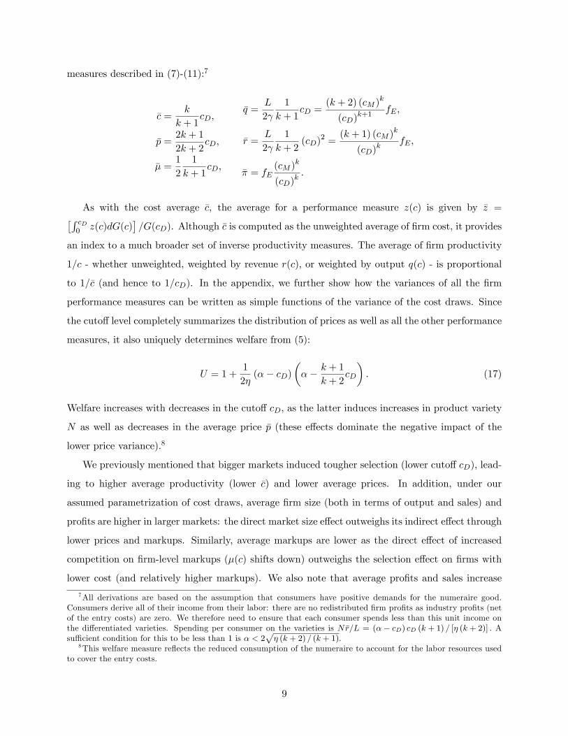
As with the cost average �c, the average for a performance measure z(c) is given by �z =�R cD0 z(c)dG(c)
�=G(cD). Although �c is computed as the unweighted average of �rm cost, it provides
an index to a much broader set of inverse productivity measures. The average of �rm productivity
1=c - whether unweighted, weighted by revenue r(c); or weighted by output q(c) - is proportional
to 1=�c (and hence to 1=cD). In the appendix, we further show how the variances of all the �rm
performance measures can be written as simple functions of the variance of the cost draws. Since
the cuto¤ level completely summarizes the distribution of prices as well as all the other performance
measures, it also uniquely determines welfare from (5):
U = 1 +1
2�(�� cD)
��� k + 1
k + 2cD
�: (17)
Welfare increases with decreases in the cuto¤ cD, as the latter induces increases in product variety
N as well as decreases in the average price �p (these e¤ects dominate the negative impact of the
lower price variance).8
We previously mentioned that bigger markets induced tougher selection (lower cuto¤ cD), lead-
ing to higher average productivity (lower �c) and lower average prices. In addition, under our
assumed parametrization of cost draws, average �rm size (both in terms of output and sales) and
pro�ts are higher in larger markets: the direct market size e¤ect outweighs its indirect e¤ect through
lower prices and markups. Similarly, average markups are lower as the direct e¤ect of increased
competition on �rm-level markups (�(c) shifts down) outweighs the selection e¤ect on �rms with
lower cost (and relatively higher markups). We also note that average pro�ts and sales increase
7All derivations are based on the assumption that consumers have positive demands for the numeraire good.Consumers derive all of their income from their labor: there are no redistributed �rm pro�ts as industry pro�ts (netof the entry costs) are zero. We therefore need to ensure that each consumer spends less than this unit income onthe di¤erentiated varieties. Spending per consumer on the varieties is N�r=L = (�� cD) cD (k + 1) = [� (k + 2)] : Asu¢ cient condition for this to be less than 1 is � < 2
p� (k + 2) = (k + 1).
8This welfare measure re�ects the reduced consumption of the numeraire to account for the labor resources usedto cover the entry costs.
9
by the same proportion when market size increases. Thus, average industry pro�tability ��=�r does
not vary with market size. Finally, we note that our technology parametrization also allows us to
unambiguously sign the e¤ects of market size on the dispersion of the �rm performance measures:
the variance of cost, prices, and markups are lower in bigger markets (the selection e¤ect decreases
the support of these distributions for any distribution G(c)); on the other hand, the variance of �rm
size (in terms of either output or revenue) is larger in bigger markets due to the direct magnifying
e¤ect of market size on these variables.
These comparative statics for the e¤ects of market size on the mean and variance of �rm per-
formance measures accord well with the empirical evidence for U.S. establishments/plants (across
regions) reported by Campbell and Hopenhayn (2005) and Syverson (2004, forthcoming). These
studies focus on sectors (retail, concrete, cement) where U.S. regional markets are relatively closed
�and focus on the e¤ects of U.S. market size (across regions) on the distribution of U.S. establish-
ments. Campbell and Hopenhayn (2005) report that retail establishments in larger markets exhibit
higher sales and employment, and �nd weaker evidence that these distributions are more disperse.
Syverson(2004, forthcoming) focuses on sectors where physical output can be measured along with
sales (and hence prices recovered). He �nds similar evidence of larger average plant size in larger
markets along with higher average plant productivity. He �nds further support for the tougher
selection e¤ect in the larger markets: the distribution of productivity is less disperse, with a higher
lower bound for the productivity distribution. These e¤ects also show up in the distribution of
plant level prices: average prices are lower in bigger markets, while the dispersion is reduced.
2.5 A Short-Run Equilibrium
In the following sections, we introduce an open economy version of our model and analyze the
consequences of various trade liberalization scenarios. The asymmetric liberalization scenarios
induce a well-known relocation of �rms (entrants in our model) across countries. We will then want
to separate these �long-run�e¤ects from the direct �short-run�e¤ects of liberalization on competition
and selection across markets. Towards this goal, we introduce a short-run version of our model.
For now, we describe its main features and equilibrium characteristics in the closed economy.
Up to this point, we have considered a long-run scenario where entry and exit decisions were
endogenously determined. In contrast, the short-run is characterized by a �xed number and dis-
tribution of incumbents. In this time frame, these incumbents decide whether they should operate
and produce �or shut down. If so, they can restart production without incurring the entry cost
10
again. No entry is possible in the short-run.
Let �N denote the �xed number of incumbents and �G(c) their cost distribution with support
[0; �cM ]. We maintain our Pareto parametrization assumption for productivity 1=c, implying �G(c) =
(c=�cM )k. As was the case in the long-run, only �rms earning non-negative pro�ts produce. This
leads to the same determination of the cost cuto¤ cD. Firms with cost c > cD shut down and the
remaining N = �N �G(cD) = �N (cD=�cM )k �rms produce. If the least productive �rm with cost �cM
earns non-negative pro�ts, then cD = �cM and all �rms produce in the short-run. Otherwise, the
cuto¤ cD is determined by the zero cuto¤ pro�t condition (13):
N =2
�
�� cDcD � �c
=2 (k + 1)
�
�� cDcD
; whenever cD < �cM ;
since the average cost of producing �rms is still �c = [k= (k + 1)] cD as in the long-run equilibrium.
Using the new condition for the number of �rms N = �N (cD=�cM )k, the zero cuto¤ pro�t condition
yields(cD)
k+1
�� cD=2 (k + 1) (�cM )
k
� �N; whenever cD < �cM ;
which uniquely identi�es the short-run cuto¤ cD and the number of producing �rms N .
In this short-run equilibrium, changes in market size do not induce any changes in the distrib-
ution of producing �rms (cD remains constant), nor in the distribution of prices and markups (see
(7) and (8)). All �rms adjust their output levels in proportion to the market size change.9 Only
entry in the long run induces inter-�rm reallocations (and the associated change in the cuto¤ cD).
3 Open Economy
In the previous section we used a closed economy model to assess the e¤ects of market size on various
performance measures at the industry level. This closed economy model could be immediately
applied to a set of open economies that are perfectly integrated through trade. In this case, the
transition from autarky to free trade is equivalent to an increase in market size �which would
induce increases in average productivity and product variety, and decreases in average markups.
However, the closed-economy scenario can not be readily extended to the case of goods that are
not freely traded. Furthermore, although trade is costly, it nevertheless connects markets in ways
9When market size changes, the residual inverse demand curve rotates around the same price bound pmax. Withlinear demand curves, the marginal revenue curve rotates in such a way that the pro�t maximizing price for any givenmarginal cost remains unchanged.
11
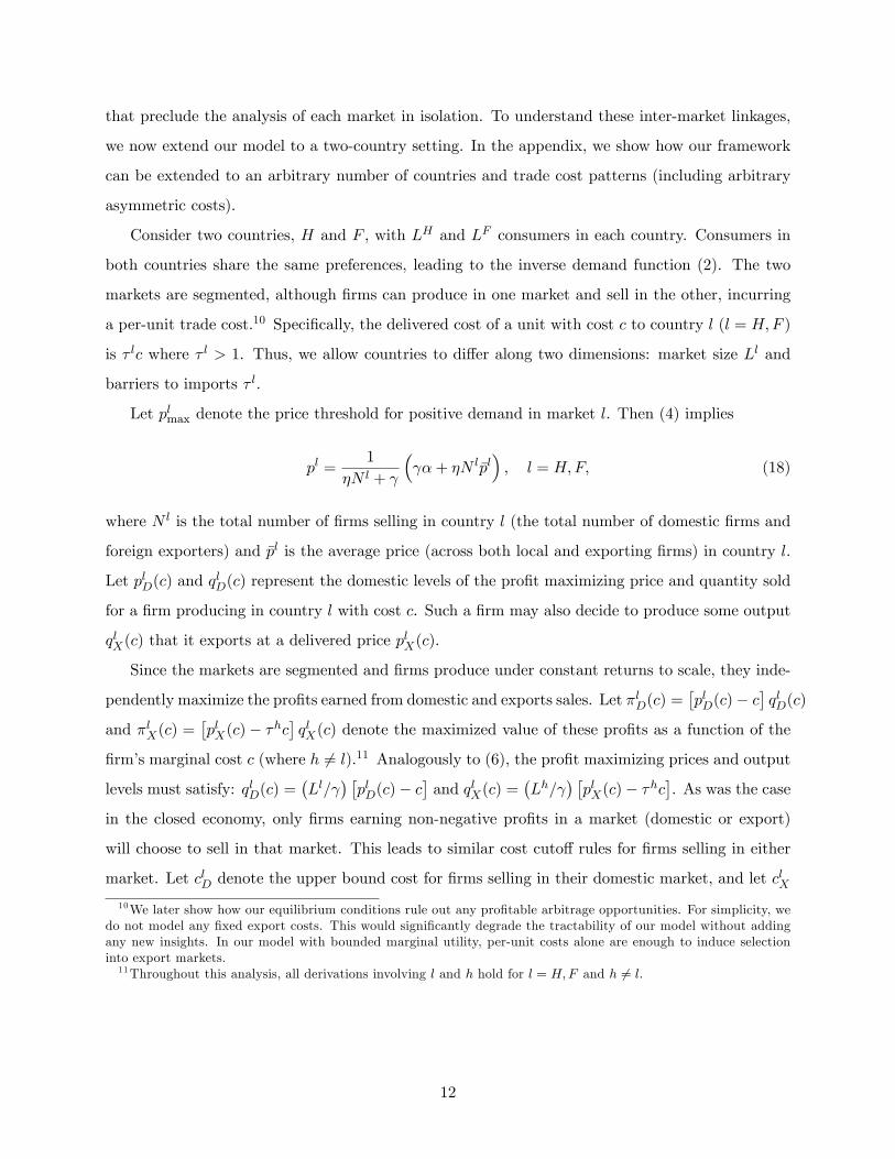
that preclude the analysis of each market in isolation. To understand these inter-market linkages,
we now extend our model to a two-country setting. In the appendix, we show how our framework
can be extended to an arbitrary number of countries and trade cost patterns (including arbitrary
asymmetric costs).
Consider two countries, H and F , with LH and LF consumers in each country. Consumers in
both countries share the same preferences, leading to the inverse demand function (2). The two
markets are segmented, although �rms can produce in one market and sell in the other, incurring
a per-unit trade cost.10 Speci�cally, the delivered cost of a unit with cost c to country l (l = H;F )
is � lc where � l > 1. Thus, we allow countries to di¤er along two dimensions: market size Ll and
barriers to imports � l.
Let plmax denote the price threshold for positive demand in market l. Then (4) implies
pl =1
�N l +
� �+ �N l�pl
�; l = H;F; (18)
where N l is the total number of �rms selling in country l (the total number of domestic �rms and
foreign exporters) and �pl is the average price (across both local and exporting �rms) in country l.
Let plD(c) and qlD(c) represent the domestic levels of the pro�t maximizing price and quantity sold
for a �rm producing in country l with cost c. Such a �rm may also decide to produce some output
qlX(c) that it exports at a delivered price plX(c).
Since the markets are segmented and �rms produce under constant returns to scale, they inde-
pendently maximize the pro�ts earned from domestic and exports sales. Let �lD(c) =�plD(c)� c
�qlD(c)
and �lX(c) =�plX(c)� �hc
�qlX(c) denote the maximized value of these pro�ts as a function of the
�rm�s marginal cost c (where h 6= l).11 Analogously to (6), the pro�t maximizing prices and output
levels must satisfy: qlD(c) =�Ll=
� �plD(c)� c
�and qlX(c) =
�Lh=
� �plX(c)� �hc
�. As was the case
in the closed economy, only �rms earning non-negative pro�ts in a market (domestic or export)
will choose to sell in that market. This leads to similar cost cuto¤ rules for �rms selling in either
market. Let clD denote the upper bound cost for �rms selling in their domestic market, and let clX
10We later show how our equilibrium conditions rule out any pro�table arbitrage opportunities. For simplicity, wedo not model any �xed export costs. This would signi�cantly degrade the tractability of our model without addingany new insights. In our model with bounded marginal utility, per-unit costs alone are enough to induce selectioninto export markets.11Throughout this analysis, all derivations involving l and h hold for l = H;F and h 6= l.
12
denote the upper bound cost for exporters from l to h: These cuto¤s must then satisfy:
clD = supnc : �lD(c) > 0
o= plmax;
clX = supnc : �lX(c) > 0
o=phmax�h
:
(19)
This implies chX = clD=�l: trade barriers make it harder for exporters to break even relative to
domestic producers.
As was the case in the closed economy, the cuto¤s summarize all the e¤ects of market conditions
relevant for �rm performance. In particular, the optimal prices and output levels can be written
as functions of the cuto¤s:
plD(c) =1
2
�clD + c
�;
plX(c) =�h
2(clX + c);
qlD(c) =Ll
2
�clD � c
�;
qlX(c) =Lh
2 �h�clX � c
�;
(20)
which yield the following maximized pro�t levels:
�lD(c) =Ll
4
�clD � c
�2;
�lX(c) =Lh
4
��h�2 �
clX � c�2:
(21)
3.1 Free Entry Condition
Entry is unrestricted in both countries. Firms choose a production location prior to entry and
paying the sunk entry cost. In order to focus our analysis on the e¤ects of market size and trade
costs di¤erences, we assume that countries share the same technology �referenced by the entry cost
fE and cost distribution G(c).12 Free entry of domestic �rms in country l implies zero expected
pro�ts in equilibrium, hence:
Z clD
0�lD(c)dG(c) +
Z clX
0�lX(c)dG(c) = fE :
12We relax this assumption in the appendix and investigate the implications of Ricardian comparative advantage.
13
We also assume the same Pareto parametrization (14) for the cost draws G(c) in both countries.
Given (21), the free entry condition can be re-written:
Ll�clD
�k+2+ Lh
��h�2 �
clX
�k+2= �; (22)
where � � 2(k + 1)(k + 2) (cM )k fE is a technology index that combines the e¤ects of better
distribution of cost draws (lower cM ) and lower entry costs fE .
This free entry condition will hold so long as there is a positive mass of domestic entrants
N lE > 0 in country l.13 In this paper, we focus on the case where both countries produce the
di¤erentiated good and N lE > 0 for l = H;F . Then, since chX = clD=�
l, the free entry condition
(22) can be re-written
Ll�clD
�k+2+ Lh�h
�chD
�k+2= �;
where �l ��� l��k 2 (0; 1) is an inverse measure of trade costs (the �freeness�of trade). This system
(for l = H;F ) can then be solved for the cuto¤s in both countries:
clD =
� �
Ll1� �h1� �l�h
� 1k+2
: (23)
3.2 Prices, Product Variety, and Welfare
The prices in country l re�ect both the domestic prices of country-l �rms, plD(c), and the prices of
exporters from h, phX(c).Using (19) and (20), these prices can be written:
plD(c) =1
2
�plmax + c
�; c 2 [0; clD];
phX(c) =1
2
�plmax + �
lc�; c 2 [0; clD=� l];
where plmax is the price threshold de�ned in (18).In addition, the cost of domestic �rms c 2 [0; clD]
and the delivered cost of exporters � lc 2 [0; clD] have identical distributions over this support, given
by Gl(c) =�c=clD
�k. The price distribution in country l of domestic �rms producing in l, plD(c),
and exporters producing in h, phX(c), are therefore also identical. The average price in country l is
thus given by
�pl =2k + 1
2k + 2clD:
13Otherwise,R clD0�lD(c)dG(c)+
R clX0
�lX(c)dG(c) < fE ; NlE = 0, and country l specializes in the numeraire. For the
sake of parsimony, we rule out this case by assuming that � is large enough.
14
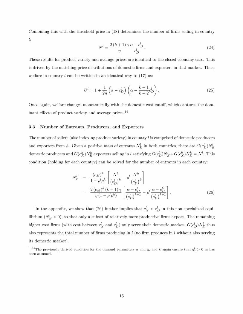
Combining this with the threshold price in (18) determines the number of �rms selling in country
l:
N l =2 (k + 1)
�
�� clDclD
: (24)
These results for product variety and average prices are identical to the closed economy case. This
is driven by the matching price distributions of domestic �rms and exporters in that market. Thus,
welfare in country l can be written in an identical way to (17) as:
U l = 1 +1
2�
��� clD
���� k + 1
k + 2clD
�: (25)
Once again, welfare changes monotonically with the domestic cost cuto¤, which captures the dom-
inant e¤ects of product variety and average prices.14
3.3 Number of Entrants, Producers, and Exporters
The number of sellers (also indexing product variety) in country l is comprised of domestic producers
and exporters from h. Given a positive mass of entrants N lE in both countries, there are G(c
lD)N
lE
domestic producers and G(chX)NhE exporters selling in l satisfying G(c
lD)N
lE+G(c
hX)N
hE = N l. This
condition (holding for each country) can be solved for the number of entrants in each country:
N lE =
(cM )k
1� �l�h
"N l�clD�k � �l Nh�
chD�k#
=2 (cM )
k (k + 1)
� (1� �l�h)
"�� clD�clD�k+1 � �l �� chD�
chD�k+1
#: (26)
In the appendix, we show that (26) further implies that clX < clD in this non-specialized equi-
librium (N lE > 0), so that only a subset of relatively more productive �rms export. The remaining
higher cost �rms (with cost between clX and clD) only serve their domestic market. G(c
lD)N
lE thus
also represents the total number of �rms producing in l (no �rm produces in l without also serving
its domestic market).
14The previously derived condition for the demand parameters � and �, and k again ensure that ql0 > 0 as hasbeen assumed.
15
3.4 Reciprocal Dumping and Arbitrage Opportunities
Brander and Krugman (1983) have shown that reciprocal dumping must occur in intra-industry
trade equilibria under Cournot competition where representative �rms produce a single homo-
geneous good in two countries. Ottaviano, Tabuchi and Thisse (2002) show that dumping can
also occur with di¤erentiated products under monopolistic competition with representative �rms.
We extend this result to our current framework, where �rms with heterogeneous costs produce
di¤erentiated varieties and face di¤erent residual demand price elasticities.15 Given the optimal
price functions plD(c) =�clD + c
�=2 and plX(c) = �h(clX + c)=2 from (20), clX < clD implies that
plX(c)=�h < plD(c); 8c � clX . Therefore, all exporters set F.O.B. export prices (net of incurred trade
costs) strictly below their prices in the domestic market. Thus, as emphasized by Weinstein (1992),
dumping does not imply predatory pricing. Furthermore, as shown by Ottaviano, Tabuchi and
Thisse (2002), dumping need not be the outcome of oligopoly and strategic interactions between
�rms, which are absent in our model.
As described by Feenstra et al (2001), dumping behavior is closely linked to arbitrage conditions
for the re-sale of goods across markets. This same link holds in our model, where dumping by
exporters from country l (plX(c)=�h < plD(c)) is equivalent to a no-arbitrage condition precluding
the pro�table export resale by a third party of a good produced and sold in country l. The dumping
condition also precludes pro�table resale of a good exported to country l, back in its origin country
h (phD(c)=�h < phX(c)).
16
3.5 The Impact of Trade
We previously described how the distribution of the exporters� delivered cost � lc to country l
matched the distribution of the domestic �rms�cost c in country l. We then argued that this would
lead to matching price distributions for both domestic �rms in a country, and exporters to that
country. This argument extends to the distribution of all the other �rm-level variables (markups,
output, revenue, and pro�t). Thus, the distribution of all these �rm performance measures in the
open economy equilibrium are identical to those in a closed economy case with a matching cost
cuto¤ cD. When analyzing the impact of trade, we can therefore focus on the determination of the
cost cuto¤ governed by (23).
15 In related work, Holmes and Stevens (2004) show that the assumption of lower markups in non-local markets,along with di¤erences in transport costs across sectors, can explain cross-market di¤erences in the size distributionof �rms.16Since phX(c) = p
lD(c�
l) > plX(c�l)=�h = phD(c�
l�h)=�h > phD(c)=�h.
16
Comparing this new cuto¤ condition to the one derived for the closed economy (15) immediately
reveals that the cost cuto¤ is lower in the open economy: trade increases aggregate productivity by
forcing the least productive �rms to exit. This e¤ect is similar to that analyzed in Melitz (2003) but
works through a di¤erent economic channel. In Melitz (2003), trade induces increased competition
for scarce labor resources as real wages are bid up by the relatively more productive �rms who ex-
pand production to serve the export markets. The increase in real wages forces the least productive
�rms to exit. In that model, import competition does not play a role in the reallocation process
due to the C.E.S. speci�cation for demand (residual demand price elasticities are exogenously �xed
and una¤ected by import competition). In the current model, the impact of these two channels �
via increased factor market or product market competition �is reversed: increased product market
competition is the only operative channel. Increased factor market competition plays no role in
the current model, as the supply of labor to the di¤erentiated goods sector is perfectly elastic. On
the other hand, import competition increases competition in the domestic product market, shifting
up residual demand price elasticities for all �rms at any given demand level. This forces the least
productive �rms to exit. This e¤ect is very similar to an increase in market size in the closed econ-
omy: the increased competition induces a downward shift in the distribution of markups across
�rms. Although only relatively more productive �rms survive (with higher markups than the less
productive �rms who exit), the average markup is reduced. The distribution of prices shifts down
due to the combined e¤ect of selection and lower markups. Again, as in the case of larger market
size in a closed economy, average �rm size and pro�ts increase �as does product variety.17 In this
model, welfare gains from trade thus come from a combination of productivity gains (via selection),
lower markups (pro-competitive e¤ect), and increased product variety.
3.6 Market Size E¤ects
We now focus on the consequences of market size di¤erences for cross-country characteristics in
the open economy equilibrium. Once again, these cross-country di¤erences in �rm performance
measures will be determined by the di¤erences in the cost cuto¤s clD, as shown in (23). This
immediately highlights how costly trade does not completely integrate markets as respective country
size plays an important role in determining all �rm performance measures and welfare in each
country: When trade costs are symmetric (�l = �h), the larger country will have a lower cuto¤,
17Comparisons of changes in the variance of all performance measures are also identical to the case of increasedmarket size.
17
and thus higher average productivity and product variety, along with lower markups and prices
(relative to the smaller country). Welfare levels are thus higher in the larger country. Moreover,
the latter will attract relatively more entrants and local producers. In short, all of the size-induced
di¤erences across countries in autarky persist (although not to the same extent). It is in this sense
that costly trade does not completely integrate markets.
Surprisingly, (23) also indicates that the size of a country�s trading partner does not a¤ect the
cost cuto¤ (and hence all �rm performance measures and welfare). This highlights some important
o¤setting e¤ects of trading partner size �although the exact outcome of these trade-o¤s are natu-
rally in�uenced by our functional form assumptions. On the export side, a larger trading partner
represents increased export market opportunities. However, this increased export market size is
o¤set by its increased �competitiveness�(a greater number of more productive �rms are competing
in that market, driving down markups). On the import side, a larger trading partner represents
an increased level of import competition. In the long run, this is o¤set by a smaller proportion of
entrants, and hence less competition in the smaller market.18
3.7 The Open Economy in the Short-Run
We now introduce the parallel version of the economy in the short-run when it is open to trade. We
will use this to separately identify the short and long run e¤ects of liberalization in the following
section. As was the case for the closed economy, no entry and exit is possible in the short run;
incumbent �rms decide whether to produce or shut-down. Each country l is thus characterized
by a �xed number of incumbents �N lD with cost distribution �Gl(c) on [0; �clM ]. We continue to
assume that productivity 1=c is distributed Pareto with shape k, implying �Gl(c) =�c=�clM
�k. A
�rm produces if it can earn non-negative pro�ts from sales to either its domestic or export market.
This leads to cost cuto¤ conditions for sales in either market: clD = sup�c : �lD(c) � 0 and c � �clM
and clX = sup
�c : �lX(c) � 0 and c � �clM
:19 Either of these cuto¤s can reach their upper bound
at �clM , in which case all incumbent �rms produce. So long as this is not the case, the cuto¤s must
18As highlighted by (26), di¤erences in country size induce a larger proportion of entrants into the larger market.(26) also indicates that country size di¤erences must be bounded to maintain an equilibrium with incomplete special-ization in the di¤erentiated good sector. As country size di¤erences become arbitrarily large, the number of entrantsin the smaller country is driven to zero.19 In the short-run, it is possible for clX > c
lD, in which case �rms with cost c in between these two cuto¤s produce
and export, but do not sell on their domestic market.
18
satisfy the threshold price conditions in (24):
N l =2 (k + 1)
�
�� clDclD
; whenever clD < �clM ; (27)
Nh =2 (k + 1)
�
�� �hclX�hclX
; whenever clX < �clM ;
where N l represents the endogenous number of sellers in country l in the short-run. Note that
chX = clD=�l as in the long-run whenever both cuto¤s are below their respective upper bounds �chM
and �clM .
There are �N lD�Gl(clD) producers from country l who sell in their domestic market, and �N
hD�Gh(chX)
exporters from h to l. These numbers must add up to the total number of sellers in country l:
N l = �N lD�Gl(clD)+
�NhD�Gh(chX). Combining this with the threshold price conditions yield expressions
This condition clearly highlights the important role played by trading partner industrial size and
import competition in the short run. An increase in the number of incumbents in country h
increases import competition in country l and generates a decreases in the cost cuto¤ clD, forcing
some of the less productive �rms in country l to shut down.20 This e¤ect is only o¤set with entry
in the long run.
4 Trade Liberalization
We have just shown how the �rm location decision (driven by free entry in the long run) plays an
important role in determining the extent of competition across markets in the open economy. This
location decision also crucially a¤ects the long run consequences of trade liberalization �especially
in situations where the decreases in trade barriers are asymmetric.
4.1 Bilateral Liberalization
Before illustrating the consequences of asymmetric liberalization, we �rst quickly describe the case
of symmetric liberalization. Here, we assume that trade costs are symmetric, �H = �F = � , and
20The overall number of sellers in country l (and hence product variety) increases as the increase in exporters fromh dominates the decrease in domestic producers in l.
19
analyze the e¤ects of decreases in � (increases in �H = �F = �). In this case, the equilibrium cuto¤
condition (23) can be written:
clD =
� �
Ll (1 + �)
� 1k+2
: (29)
Bilateral liberalization thus increases competition in both markets, leading to proportional changes
in the cuto¤s (and hence proportional increases in aggregate productivity) in both countries.21 The
e¤ects of such liberalization are thus qualitatively identical to those described for the transition from
autarky to the open economy: Product variety increases as a result of the increased competition,
which also induces a decrease in markups and prices. Again, welfare rises from a combination of
higher productivity, lower markups, and increased product variety.
Symmetric trade liberalization induces all of the same qualitative results in the short run.
Although these e¤ects do not depend on relative country size (so long as the di¤erentiated good
is produced in both countries), di¤erences in country size nevertheless induce important changes
in the relative pattern of entry in the long run following liberalization. Assuming Ll > Lh, the
positive entry di¤erential N lE�Nh
E widens with liberalization as entry in the bigger market becomes
relatively more attractive. This also induces a growing di¤erential in the number of domestic
producers N lD �Nh
D (see appendix for proofs).
4.2 Unilateral Liberalization
We now describe the e¤ects of a unilateral liberalization by country l (an increase in �l, holding
�h constant). Given the cuto¤ condition (23), this leads to an increase in the cost cuto¤ clD (less
competition in the liberalizing country) �whereas the cuto¤ chD in the country�s trading partner
decreases, indicating an increase in competition there. The liberalizing country thus experiences a
welfare loss while its trading partner experiences a welfare gain.22 As previously mentioned, these
results are driven by the change in �rm location induced by entry in the long run. (26) indicates
that the number of entrants N lE in the liberalizing country decreases, while the number of entrants
in the other country, NhE , increases.
In order to isolate the direct impact of liberalization from the long run e¤ects generated by
entry, we now turn to the short run responses to unilateral liberalization by country l. The equi-
librium condition (28) for the short run cuto¤s clearly shows that the cost cuto¤ clD decreases in
21As indicated by (26), the number of entrants in the smaller economy is driven to zero when trade costs dropbelow a threshold level �and the smaller economy no longer produces the di¤erentiated good. We assume that tradecosts remain above this threshold level.22Once again, the response of the cuto¤s determines the response in all the other country level variables.
20
response to this liberalization �while the cost cuto¤ in h, chD, remains unchanged. This highlights
the pro-competitive e¤ects of unilateral liberalization in the short-run. Although the increase in
import competition in l forces some of the least productive �rms there to exit, product variety N l
nevertheless increases as the increased number of exporters to l dominates the decrease in domestic
producers N lD (see (27)). Welfare in the liberalizing country (in the short run) therefore rises from
a combination of higher productivity, lower markups, and increased product variety (welfare in
the trading partner remains unchanged in the short run). These results clearly underline how the
welfare loss associated with unilateral liberalization is driven by the shift in the pattern of entry
(favoring the non-liberalizing trading partner) in the long run.
These long run e¤ects of liberalization on �rm �de-location�have been extensively studied in
previous work (see, e.g. Horstmann and Markusen, 1986, Venables, 1985, Venables, 1987; and the
synthesis in Helpman and Krugman, 1989 ch. 7 and Baldwin et al, 2003 ch. 12). The novel features
in our work show how this type of liberalization also a¤ects �rm selection, aggregate productivity,
product variety, and markups within a single model.23
4.3 Preferential Liberalization
So far, our analysis has been restricted to two countries. This has generated a rich set of insights on
the combined impact of market size and trade liberalization on industry performance and welfare.
However, focusing on two countries in isolation neglects the e¤ects of a country�s position within an
international trading network (which is determined by the whole matrix of bilateral trade barriers).
When all trade barriers are symmetric, the insights of a multi-country model are a straightforward
extension of the two-country case. However, new insights arise when bilateral barriers are allowed
to di¤er.
While our model can easily deal with any number of countries of any size along with an arbitrary
matrix of trade costs (see appendix), considering three countries of equal size is enough to recover
some of these related insights. We therefore introduce a third trading partner T; with LT = LH =
LF = L. Countries di¤er in terms of trade barriers that are assumed to be pair-wise symmetric,
with �lh =�� lh��k
=��hl��k
measuring the �freeness�of trade between countries l = fH;F; Tg
and h 6= l. Similarly, �lt and �ht measure the �freeness�of trade between l and h, and the third
country t 6= l 6= h. As with the case of unilateral liberalization, preferential trade liberalization
23Since most of the previous literature assumes representative �rms, the link between trade policy and aggregateproductivity (via �rm selection into the domestic market) and product variety (via �rm selection into export markets)is absent.
21
(non-proportional changes in these three bilateral trade barriers) induces important shifts in the
pattern of entry across countries in the long-run. Once again, we analyze both the long run and
short run e¤ects of such liberalization.
Long run equilibrium
With three countries of equal size, the free entry condition (22) in country l becomes:
�clD
�k+2+ �lh
�chD
�k+2+ �ht
�ctD�k+2
= �
Ll = fH;F; Tg; t 6= l 6= h:
This provides a system of three linear equations in the three domestic cuto¤s. When pair-wise
trade barriers are symmetric, the long run cuto¤s are given by:
clD =
" �
L
�1� �ht
� �1 + �ht �
��lh + �lt
��1 + 2�lh�lt�ht � (�lh)2 � (�lt)2 � (�ht)2
# 1k+2
: (30)
The corresponding number of sellers N l in country l is still given by (24), while the number of
entrants solve N lE + �
lhNhE + �
ltN tE = N l
�cM=c
lD
�k:
In (30), international di¤erences in cuto¤s stem from the relative freeness measure�1� �ht
� �1 + �ht �
��lh + �lt
��, which implies that the cuto¤ is lowest in a country l with the
lowest sum of bilateral barriers ( highest �lh + �lt). In e¤ect, this country is the best export base
or �hub�. Moreover, since �ht enters the expression of the cuto¤ for country l; any change in bilat-
eral trade costs a¤ects all three countries. This has important implications for preferential trade
agreements.24 To see this as clearly as possible, consider three countries with initially symmetric
trade barriers (�lt = �). The initial cuto¤s are then identical and equal to (see (30))
cD =
� �
L
1
1 + 2�
� 1k+2
: (31)
A preferential trade agreement is then introduced between H and F; inducing �HF = �0 > � =
�FT = �HT . The new trade regime a¤ects the cuto¤s for all countries. From (30), the cuto¤s in
the liberalizing countries are then
cHD = cFD =
� �
L
1� �1� 2�2 + �0
� 1k+2
; (32)
24 In the appendix, we show how such �third-country e¤ect�can also be integrated in a gravity equation.
22
while the cuto¤ in the third country is given by
cTD =
� �
L
(1� �) + (�0 � �)1� 2�2 + �0
� 1k+2
: (33)
The number of entrants in all three countries are given by (recall that cHD = cFD)
NHE = NF
E =2 (cM )
k (k + 1)
� (1� 2�2 + �0)
"�� cHD�cHD�k+1 � � �� cTD�
cTD�k+1
#;
NTE =
2 (cM )k (k + 1)
� (1� 2�2 + �0)
"�1 + �0
� �� cTD�cTD�k+1 � 2� �� cHD�
cHD�k+1
#:
Comparing (31)-(33), it is easily veri�ed that preferential liberalization leads to lower cuto¤s
in the liberalizing countries and a higher cuto¤ in the third country. Thus, average costs, prices,
and markups also decrease in the liberalizing countries while they rise in the third country. The
liberalizing countries become better �export bases�: they gain better access to each other�s market
while maintaining the same ease of access to the third country�s market. Thus, preferential liber-
alization leads to long run welfare gains for the liberalizing countries, along with a welfare loss for
the excluded country.
Short run
In order to highlight how the welfare loss in the third country is driven by the long run shift in
the pattern of entry, we brie�y characterize the short run response to the liberalization agreement
between H and F . The short run equilibrium in country l solves:
�� clD�clD�k+1 = �
2(k + 1)
"NlD�
clM�k + �lh N
hD�
chM�k + �lt N
tD�
ctM�k#;
where the number of incumbents �N lD and their productivity distribution on [0; �clM ] are �xed in
all countries, as in the previous short run examples. When these numbers and distributions are
symmetric (same �N and �cM ), the country with the best accessibility (highest �hl + �lt) will have
the lowest cuto¤ clD. This country will have the lowest number of operating �rms NlD =
�N lDG(c
lD),
but the highest number of sellers N l (see (27)). Since the preferential liberalization between H
and F does not a¤ect accessibility to the third country (� = �FT = �HT ), the cuto¤ in the
latter is una¤ected by the preferential liberalization in the short run. As in the case of unilateral
23
liberalization, it is the long run change in entry behavior that is responsible for reduced competition
and lower welfare in the excluded third country. On the other hand, the liberalizing countries gain in
both the short run (via the direct pro-competitive e¤ect) and the long run, when the pro-competitive
e¤ect is reinforced by the bene�cial impact of increased entry.
5 Conclusion
We have presented a rich, though tractable, model that predicts how a wide set of industry per-
formance measures (productivity, size, price, markup) respond to changes in the world trading
environment. Our model incorporates heterogeneous �rms and endogenous markups that respond
to the toughness of competition in a market. In such a setting, we show how market size induces
important changes in industry performance measures: larger markets exhibit tougher competition
resulting in lower average markups and higher aggregate productivity. We also show how costly
trade does not completely integrate markets and thus does not obviate these important conse-
quences of market size di¤erences across trading partners.
We then analyze several di¤erent trade liberalization scenarios. Our model highlights the pro-
competitive e¤ects of increased import competition and its e¤ect on markups, productivity, and
product variety in the liberalized import market. Our model also echoes the �ndings in previous
work that show how the short run gains of asymmetric liberalization can be reversed by shifts in
the pattern of entry in the long run. However, our model additionally incorporates the important
feedbacks between entry and �rm selection into domestic and export markets.
Although each of these individual channels for trade-induced gains have been previously an-
alyzed in models with di¤erent structures, we believe it is important to show how all of these
channels can be captured within a single uni�ed framework. This framework develops a new and
very tractable way of describing how di¤erences in market size and trade costs across trading part-
ners a¤ect the distribution of key �rm-level performance measures across markets. We hope that
this provides a useful foundation for future empirical investigations.
References
[1] Asplund, M. and V. Nocke (2006) Firm Turnover in Imperfectly Competitive Markets, Reviewof Economic Studies 73, 295-327.
24
[2] Aw, B. Y., S. Chung and M. J. Roberts (2000) Productivity and Turnover in the ExportMarket: Micro-level Evidence from the Republic of Korea and Taiwan (China). World BankEconomic Review 14, 65-90.
[3] Bernard, A. B., J. Eaton, J. B. Jensen, and S. Kortum (2003), Plants and Productivity inInternational Trade, American Economic Review 93, 1268-1290.
[4] Bernard, A. and B. Jensen (1999) Exceptional Exporter Performance: Cause, E¤ect, or Both?,Journal of International Economics 47, 1-25.
[5] Bernard, A. B., J. B. Jensen, and P. K. Schott (2006) Trade Costs, Firms and Productivity,Journal of Monetary Economics 53, 917-37.
[6] Brander, J. and P. Krugman (1983) A �Reciprocal Dumping�Model of International Trade,Journal of International Economics 15, 313-21.
[7] Campbell, J. and H. Hopenhayn (2005) Market size matters, Journal of Industrial Economics53, 1-25.
[8] Clerides, S.K., S. Lach and J. R. Tybout (1998) Is Learning by Exporting Important? Micro-dynamic Evidence from Colombia, Mexico, and Morocco. The Quarterly Journal of Economics113, 903-47.
[9] Combes, P., G. Duranton, L. Gobillon, D. Puga, and S. Roux (2007) The Productivity Advan-tage of Large Markets: Distinguishing Agglomeration from Firm Selection, mimeo, Universityof Toronto.
[10] Del Gatto, M., G. Mion, and G.I.P. Ottaviano (2006) Trade Integration, Firm Selection andthe Costs of Non-Europe, University of Bologna, mimeo.
[11] Eaton, J., and S. Kortum (2002) Technology, Geography, and Trade, Econometrica 70, 1741-1779.
[12] Feenstra, R., J. Markusen, and A. Rose (2001)Using the Gravity Equation to Di¤erentiateAmong Alternative Theories of Trade, Canadian Journal of Economics 34, 430-447.
[13] Helpman, E. and P. Krugman (1989) Trade Policy and Market Structure, MIT Press.
[14] Helpman, E., M. J. Melitz, and Y. Rubinstein (2007) Estimating Trade Flows: Trading Part-ners and Trading Volumes, NBER Working Paper No. 12927.
[15] Holmes, T., and J. Stevens (2004), Geographic Concentration and Establishment Size: Analysisin an Alternative Economic Geography Model, Journal of Economic Geography 4, 227-50.
[16] Horstmann, I. J., and J. R. Markusen (1986) Up the Average Cost Curve: Ine¢ cient Entryand the New Protectionism, Journal of International Economics 20, 225-47.
[17] Krugman, P. R. (1979) Increasing Returns, Monopolistic Competition, and InternationalTrade, Journal of International Economics 9, 469-79.
[18] Krugman, P. R. (1980) Scale Economies, Product Di¤erentiation, and the Pattern of Trade,American Economic Review 70, 950-9.
25
[19] Markusen, J. R. (1981) Trade and the Gains from Trade with International Competition,Journal of International Economics 11, 531-51.
[20] Melitz, M.J. (2003) The Impact of Trade on Intra-Industry Reallocations and Aggregate In-dustry Productivity. Econometrica 71, 1695-1725.
[21] Ottaviano, G.I.P., T. Tabuchi and J.-F. Thisse (2002) Agglomeration and Trade Revisited,International Economic Review 43, 409-436.
[22] Pavcnik, N. (2002) Trade Liberalization, Exit, and Productivity Improvements: Evidence fromChilean Plants, Review of Economic Studies 69, 245-276.
[23] Syverson, C. (2004) Market Structure and Productivity: A Concrete Example. Journal ofPolitical Economy 112, 1181-1222.
[24] Syverson, C. (forthcoming) Prices, Spatial Competition, and Heterogeneous Producers: AnEmpirical Test, Journal of Industrial Economics, forthcoming.
[25] Tybout, J. (2002) Plant and Firm-Level Evidence on New Trade Theories. In Handbook ofInternational Economics, J. Harrigan (ed.), Vol. 38, Basil-Blackwell.
[26] Venables, A. J. (1985) Trade and Trade Policy with Imperfect Competition: The Case ofIdentical Products and Free Entry, Journal of International Economics 19, 1-19.
[27] Venables, A.J. (1987) Trade and Trade Policy with Di¤erentiated Products: A Chamberlinian-Ricardian model, Economic Journal 97, 700-717.
[28] Weinstein, D. (1992) Competition and Unilateral Dumping. Journal of International Economics32, 379-388.
26
Appendix
A Variance of Firm Performance Measures
Let �2c =hR cD0 (c� �c)2 dG(c)
i=G(cD) denote the variance of the �rm cost draws. As was mentioned
earlier in the main text, the variance of all the �rm performance measures can be written as simple
expressions of this variance:
�2p =14�
2c ; �2q =
L2
4 2�2c ;
�2� =14�
2c ; �2r =
L2
16 2�2c2 ;
where �2z =hR cD0 [z(c)� �z]2 dG(c)
i=G(cD) and �z denote the variance and mean of a �rm perfor-
mance measure z(c). Given the chosen parametrization for the cost draws, �2c =�k=(k + 1)2(k + 2)
�c2D.
B Multiple Countries, Asymmetric Trade Costs, and Comparative Advantage
Our model can be readily extended to a setting with an arbitrary number of countries, asymmetric
trade costs, and comparative advantage. Let M denote the number of countries, indexed by l =
1; :::;M . As in the main text �lh =�� lh��k 2 (0; 1] measures the �freeness�of trade for exports from
l to h. When trade costs are interpreted in a wide sense as all distance-related barriers, then within
country trade may not be costless, and we allow for any �ll 2 (0; 1]. We introduce comparative
advantage as technology di¤erences that a¤ect the distribution of the �rm-level productivity draws.
For tractability, we assume that �rm productivity 1=c is distributed Pareto with shape k in all
countries, but allow for di¤erences in the support of the distributions via di¤erences in the upper-
bound cost clM . The cost draws in country l thus have a distribution Gl(c) =
�c=clM
�k. Whenever
clM < chM , country l will have a comparative advantage with respect to country h in the di¤erentiated
good sector: entrants in country l have a better chance of getting higher productivity draws.25
In this extended model, the free entry condition (22) in country l becomes:
MXh=1
�lhLh�chD
�k+2=2 (k + 1)(k + 2)fE
ll = 1; :::;M;
where l =�clM��k
is an index of comparative advantage. This yields a system of M equations
25The distribution of productivity draws in l stochastically dominates that in h.
A-1
that can be solved for the M equilibrium domestic cuto¤s using Cramer�s rule:
clD =
2(k + 1)(k + 2)fE
jP j
PMh=1 jChlj = h
Ll
! 1k+2
; (B.1)
where jP j is the determinant of the trade freeness matrix
P �
0BBBBBB@�11 �12 � � � �1M
�21 �22 � � � �2M...
.... . .
...
�M1 �M2 � � � �MM
1CCCCCCA ;
and jChlj is the cofactor of its �hl element. Cross-country di¤erences in cuto¤s now arise from
three sources: own country size (Ll), as well as a combination of market access and comparative
advantage (PMh=1 jChlj = h). Countries bene�ting from a larger local market, a better distribution
of productivity draws, and better market accessibility have lower cuto¤s.
The mass of sellers N l in each country l (including domestic producers in l and exporters to l)
is still given by (24). Given a positive mass of entrants N lE in all countries, there are G
l(clD)NlE
domestic producers andPh 6=lG
l(chlX)NhE exporters selling in l, where c
hlX is the export cuto¤ from
h to l. This implies:MXh=1
�hl hNhE =
N l�clD�k :
The latter provides a system of M linear equations that can be solved for the number of entrants
in the M countries using Cramer�s rule:26
N lE =
2 (k + 1)
� jP j lMXh=1
��� chD
�jClhj�
chD�k+1 (B.2)
Given N lE entrants in country l, N
lEG
l(clD) �rms survive and produce for the local market. Among
the latter, N lEG
l(clX) export to country h.
C A Gravity Equation
Our multilateral model with heterogeneous �rms, asymmetric trade costs, and comparative advan-
tage also yields a gravity equation for aggregate bilateral trade �ows. An exporter with cost c from
26We use the properties that relate the freeness matrix P and its transpose in terms of determinants and cofactors.
A-2
country h generates export sales rlhX (c) = plhX(c)qlhX (c) where (see (19) and (20))
plhX(c) =� lh
2
�clhX + c
�=1
2
�chD + �
lhc�;
qlhX (c) =Lh� lh
2
�clhX � c
�=Lh
2
�chD � � lhc
�:
Aggregating these export sales rlhX (c) over all exporters from l to h (with cost c � clhX) yields the
aggregate bilateral exports from l to h:27
EXP lh = N lE
Z clhX
0rlhX (c)dG
l(c)
= N lE
Lh
4
Z chD=�lh
0
��chD
�2��� lhc
�2�dGl(c)
=1
2 (k + 2)N lE
lLh�chD
�k+2 �� lh��k
: (C.1)
This gravity equation determines bilateral exports as a log-linear function of bilateral trade barriers
and country characteristics. As in Eaton and Kortum (2002) and Helpman, Melitz, and Rubinstein
(2007), (C.1) re�ects the joint e¤ects of country size, technology (comparative advantage), and
geography on both the extensive (number of traded goods) and intensive (amount traded per good)
margins of trade �ows. Similarly, (C.1) highlights how �holding the importing country size �xed
� tougher competition in that country (lower average prices, re�ected by a lower clD) dampens
exports by making it harder for potential exporters to break into that market.
D Selection Into Export Markets
In this section, we show that the assumption of a non-specialized equilibrium where both countries
produce the di¤erentiated good (N lE > 0; l = H;F ) implies that only a subset of relatively more
productive �rms choose to export in either country (clX < clD; l = H;F ). In the text, we showed
27The integration measure Gl(clhX ) represents the proportion of entrants NlE in l that export to h.
A-3
that the number of entrants N lE satis�ed (26). Thus,
N lE > 0 () �� clD�
clD�k+1 > �l
�� chD�chD�k+1
() �� clD�� chD
�chDclD
�k+1> �l
()�� l� chX
�� chD
�chDchX
�k+1> 1;
which is incompatible with chX � chD. Therefore, chX < chD for h = H;F .
E Bilateral Liberalization
In this section, we prove a set of results for the two country model with di¤erent country sizes
and symmetric trade barriers. Some results are already mentioned in the main text, while oth-
ers complement the latter and provide a more detailed characterization of the e¤ects of bilateral
liberalization.
When trade barriers are symmetric, �l = �h = �, the number of entrants from (26) can be
simpli�ed to:
N lE =
(cM )k
1� �2
"N l�clD�k � � Nh�
chD�k#: (E.1)
Among these entrants, only
N lD = G(clD)N
lE =
�clDcM
�kN lE (E.2)
�rms survive and produce. Without loss of generality, we assume Ll > Lh. The following results
then apply:
1. The domestic cuto¤ is lower in the larger country: clD < chD. Proof : Follows directly from
(29).
2. There are more sellers in the larger country: N l > Nh. Proof : Given 1, follows directly from
(24).
3. There are more entrants in the larger country: N lE > Nh
E . Proof : Given 1 and 2, follows
directly from (E.1).
A-4
4. There are more local producers in the larger country: N lD > Nh