THE JOURNAL OF FINANCE • VOL. LIX, NO. 3 • JUNE 2004

Market States and Momentum

MICHAEL J. COOPER, ROBERTO C. GUTIERREZ JR.,and ALLAUDEEN HAMEED∗

ABSTRACT

We test overreaction theories of short-run momentum and long-run reversal in thecross section of stock returns. Momentum profits depend on the state of the market,as predicted. From 1929 to 1995, the mean monthly momentum profit following pos-itive market returns is 0.93%, whereas the mean profit following negative marketreturns is −0.37%. The up-market momentum reverses in the long-run. Our resultsare robust to the conditioning information in macroeconomic factors. Moreover, wefind that macroeconomic factors are unable to explain momentum profits after simplemethodological adjustments to take account of microstructure concerns.

SEVERAL BEHAVIORAL THEORIES have been developed to jointly explain the short-run cross-sectional momentum in stock returns documented by Jegadeesh andTitman (1993) and the long-run cross-sectional reversal in stock returns doc-umented by DeBondt and Thaler (1985).1 Daniel, Hirshleifer, and Subrah-manyam (1998; hereafter DHS) and Hong and Stein (1999; hereafter HS) eachemploy different behavioral or cognitive biases to explain these anomalies.2,3

∗Cooper is from the Krannert Graduate School of Management, Purdue University. Gutierrez isfrom the Lundquist College of Business, University of Oregon. Hameed is from the NUS BusinessSchool, National University of Singapore. We gratefully acknowledge financial support from theJohn and Mary Willis research award (Cooper), a Summer Research Grant from the Department ofFinance at Texas A&M (Gutierrez), and an Academic Research Grant from the National Universityof Singapore (Hameed). We thank Kent Daniel, Ken French, Simon Gervais, Eric Ghysels, ChristoPirinsky, Bhaskaran Swaminathan, and seminar participants at the University of Colorodo, Uni-versity of Utah, and University of Virginia for their helpful discussions. Comments from the editor,Rick Green, and an anonymous referee are also gratefully acknowledged. Any errors are our own.

1 We use the phrase “short-run” to refer to six- to twelve-month momentum for ease of exposition.Note that the behavioral models do not address the shorter-run evidence of reversal at the weeklyhorizon (Lehmann (1990), Lo and MacKinlay (1990), Cooper (1999)).

2 Our understanding is that the predictions of the Barberis, Shleifer, and Vishny (1998) model formomentum profits conditioned on the state of the market are difficult to assess, which is the centraltest of our study as we soon discuss. In their model, individuals typically overreact (underreact)to low-weight, high-strength news (high-weight, low-strength news). Testing this model requiresidentifying and characterizing news in terms of their “strength” and “weight”.

3 The three-factor model of Fama and French (1996) can explain long-run reversal but not short-run momentum. Ahn, Conrad, and Dittmar (2002) and Yao (2002) employ nonparametric methodsand show that systematic factors explain momentum. To the extent that mispricings are system-atic, however, the basis assets themselves may also be capturing irrationalities (Hirshleifer (2001)).Additionally, Lee and Swaminathan (2000) show that trading volume plays a role in the profits tomomentum strategies, which they interpret to mean that prices generally deviate from fundamen-tal values. Grinblatt and Moskowitz (2003) conclude that tax environments affect the profits to

1345

1346 The Journal of Finance

Following these models, we test the theory that overreaction is the source ofthese return patterns.

DHS assume that investors are overconfident about their private informa-tion and overreact to it. If investors also have a self-attribution bias, then whensubsequent (public) information arrives, investors will react asymmetricallyto confirming versus disconfirming pieces of news. In other words, investorsattribute successes to their own skill more than they should and attribute fail-ures to external noise more than they should. The consequence of this behav-ior is that investors’ overconfidence increases following the arrival of confirm-ing news. The increase in overconfidence furthers the initial overreaction andgenerates return momentum. The overreaction in prices will eventually be cor-rected in the long-run as investors observe future news and realize their errors.Hence, increased overconfidence results in short-run momentum and long-runreversal.

The theory of DHS can be extended to predict differences in momentum prof-its across states of the market. Aggregate overconfidence should be greater fol-lowing market gains (DHS and Gervais and Odean (2001)). Since investors inaggregate hold long positions in the equity market, increases in market priceswill tend to be attributed unduly to investor skill and will result in greateraggregate overconfidence. If overconfidence is in fact higher following marketincreases, then the overreactions will be stronger following these up marketsgenerating greater momentum in the short-run.

HS also develop a behavioral theory to explain momentum. Their model isbased on initial underreaction to information and subsequent overreaction,which eventually leads to stock price reversal in the long-run. The HS modelemploys two types of investors: “newswatchers” and “momentum traders.” Thenewswatchers rely exclusively on their private information; momentum tradersrely exclusively on the information in past price changes. The additional as-sumption that private information diffuses only gradually through the mar-ketplace leads to an initial underreaction to news.4 The underreaction andsubsequent positive serial correlation in returns attracts the attention of themomentum traders whose trading activity results in an eventual overreactionto news. Prices revert to their fundamental levels in the long-run.

This model also predicts relative changes in price dynamics depending on thestate of the market. HS examine the effect of changing the risk aversion of mo-mentum traders. In their Figure 2, they found that decreasing risk aversion ledto greater delayed overreaction, and therefore, to increased momentum profits.To the extent that risk aversion decreases as wealth increases (as suggestedby Campbell and Cochrane (1999), Barberis, Huang, and Santos (2001), and

both momentum and contrarian strategies. Lesmond, Schill, and Zhou (2002) and Korajczyk andSadka (2002) question if momentum profits are realizable given trading costs. Finally, the concernfor a data-snooping bias seems small given the foreign-market evidence of Rouwenhorst (1998) andthe 1990s United States evidence of Jegadeesh and Titman (2001).

4 Holden and Subrahmanyam (2002) also develop a model that generates momentum throughthe gradual diffusion of information.

Market States and Momentum 1347

others), this model also predicts that momentum profits will be greater follow-ing market gains.

We examine whether conditioning on the state of the market is importantto the profitability of momentum strategies. We define two states: (1) “UP” iswhen the lagged three-year market return is non-negative, and (2) “DOWN” iswhen the three-year lagged market return is negative. We find that short-runmomentum profits exclusively follow UP periods. From 1929 through 1995, thesix-month momentum strategy generates a significant mean monthly profit of0.93% after three-year UP markets and an insignificant −0.37% profit afterthree-year DOWN markets. Furthermore, these profits are significantly differ-ent, and these results are robust using one-year and two-year lagged marketstates and risk adjustments. Hence, consistent with DHS and HS, the state ofthe market is critically important to the profitability of momentum strategies.

A central prediction of the overreaction theory is that the momentum profitswill reverse in the long-run as the market eventually corrects the mispric-ings. Similar to the unconditional results in Lee and Swaminathan (2000) andJegadeesh and Titman (2001), we find that UP-market momentum profits dosignificantly reverse in the long-run. The mean return spread between priorwinners and losers over holding-period months 13 to 60 is reliably negative at–0.36% per month following UP market states. So when there is momentum,there is ultimately long-run reversal.

Interestingly, we also find significant long-run reversal following DOWNstates as well, despite the absence of DOWN-state momentum in the short-run. This finding is not necessarily inconsistent with the overreaction theoriesof momentum, since there may be other factors causing long-run reversal ingeneral. For example, it may be that cyclical variations in risk drive a portionof the long-run reversal. While we are sympathetic with the intuition behindtime variation in risk, it is important to note that there is concern over how tomodel such variation. Ghysels (1998) forcefully shows that popular methods ofmodeling variation in risk do not lead to improvements over static risk models.5

One implication of our findings is that long-run reversals are not solely due tothe corrections of prior momentum. Although overreaction does not seem toentirely explain the lagged-return anomalies, it does seem to explain a largeportion of the momentum and reversal patterns.

The finding that momentum is dependent on the state of the market seemsrelated to the recent evidence of Chordia and Shivakumar (2002; hereafterCS) that commonly used macroeconomic instruments for measuring marketconditions can explain a large portion of momentum profits. CS argue thatintertemporal variations in the macroeconomic factors (and presumably risk)

5 Additionally, there are other psychological biases that might explain long-run reversal followingDOWN states. Specifically, Daniel, Hirshleifer, and Teoh (2002) note that investors might have asalience bias. Given the increased coverage the media gives to the stock market during recessions,investors may tend to overreact to news in these bad times, only because of the greater saliency ofthe news.

1348 The Journal of Finance

are the main sources of momentum profits. We examine if such a multifactormodel can explain the asymmetry in momentum profits across UP and DOWNmarkets. Dividend yield, default spread, term spread, and short-term inter-est rates do not capture the asymmetry in momentum profits. Additional testsindicate that the success of the macroeconomic multifactor model in explain-ing momentum documented by CS is not robust to common screens used tomitigate microstructure-induced biases. Specifically, the employment of a one-dollar price screen (to remove highly illiquid and high-trading-cost stocks) orthe skipping of the month between the formation period and the trading period(to minimize spurious negative autocorrelation due to bid–ask bounce) reversesthe findings of CS that the macroeconomic model can explain momentum.6

In addition, we consider if the market state is informative about momen-tum profits beyond the two-state, UP and DOWN, conditioning set we initiallyconsider. In other words, we examine if momentum profits are greatest whenthe market’s state is highest. There is a nonlinear relation between momen-tum profits and lagged market states. As the lagged market return increases,momentum increases and reaches a peak near the median level of market per-formance, slowly declining thereafter. When the lagged market return is high-est, however, there remain significant momentum profits. We discuss potentialexplanations of this nonlinearity. Lastly, using a recursive out-of-sample proce-dure, we find that the lagged return on the market is a robust predictor of thetime-series of momentum profits, while the macroeconomic multifactor modelis not.

In sum, the state of the market measured using the lagged market return con-tains information about the profitability of momentum strategies. The remain-ing sections are organized as follows. Section I details the data and methodologyand presents the momentum profits in the short-run and long-run across UPand DOWN market states; Section II provides several robustness checks andadditional discussions of the main findings, including controlling for a macroe-conomic factor model similar to Chordia and Shivakumar (2002); and Section IIIconcludes the paper.

I. Analysis of Profits across States

A. Data and Method

The data for the study are all NYSE and AMEX stocks listed on the CRSPmonthly file. Our sample period covers January 1926 to December 1995. Stocksare sorted at the end of each month t into deciles based on their prior six-month returns. To mitigate bid–ask bounce effects, the formation-period six-month returns are calculated from t − 5 to t − 1, skipping month t. We excludestocks with a price at the end of the formation period below $1 to mitigate

6 Jegadeesh and Titman (1993, 2001) and Fama and French (1996), among others, have employedsuch filters to better estimate momentum profits. Recently, Griffin, Ji, and Martin (2003) questionthe ability of macroeconomic models to explain momentum in foreign stock returns.

Market States and Momentum 1349

microstructure effects associated with low-price stocks. The test-period profitsare calculated for three holding periods, t + 1 to t + 6, t + 1 to t + 12, and t + 13to t + 60, as follows. We define each momentum portfolio as long in the prior six-month winners (highest decile) and short in the prior six-month losers (lowestdecile). We form a time-series of raw profits corresponding to each event monthof the holding period, that is, we form 60 time-series of profits correspondingrespectively to month 1, month 2, . . . , month 60. To form the CAPM and Fama–French (1993) risk-adjusted profits, for each holding-period month, we regressthe time-series of raw profits on the appropriate factors and a constant. Thus,we obtain the estimated factor loadings for each holding-period-month series.The risk-adjusted profits are

radjkt = rkt −

∑

i

β̂ik fit , (1)

where rkt is the raw profit for the strategy in holding-period month k, for k =1, 2, . . . , 60, in calendar month t, fit is the realization of factor i in calendarmonth t, and β̂ik is the estimated loading of the time-series of raw profits inholding-period-month k on fit. We use the excess return of the value-weightedmarket index over the one-month T-bill return as the sole factor for the CAPMrisk adjustments and two additional factors, the small-minus-big return pre-mium (SMB) and the high-book-to-market-minus-low-book-to-market returnpremium (HML), for the Fama–French risk adjustments.7

The monthly raw, CAPM-adjusted, or Fama–French-adjusted profits are thencumulated to form the holding-period profits (CAR):

CARt+K2 =K2∑

k=K1

r∗k,t+k , (2)

where r∗ is either raw (rkt) or risk-adjusted (radjkt ) profits and the (K1, K2) pairs

are (1, 6), (1, 12), and (13, 60). For example, for the month of June 1980, theCAR over holding-period months 1 to 6 is the sum of the monthly raw or risk-adjusted profits from January, February, March, April, May, and June of 1980,where the profit used in each of these months is from holding-period months1, 2, 3, 4, 5, and 6, respectively; and the six-month momentum portfolio in thiscase is formed at the end of November 1979 (skipping December). The CARperformance metric above is similar to ones employed by Jegadeesh and Titman(1993, Tables VII and VIII) and Nagel (2001). Since the CARs are overlapping,we employ a heteroskedasticity-and-autocorrelation-consistent (HAC) estimateof the variance (Gallant (1987)), setting the number of lags equal to the numberof overlapping months in the holding-period window (5, 11, or 47).8

7 We thank Ken French for providing the time-series of data for the Fama–French three-factormodel. These factors are described by Fama and French (1993).

8 We have replicated our tests using six-month nonoverlapping CARs (starting in January/Julyand March/September) and find that our results hold.

1350 The Journal of Finance

As discussed earlier, the overreaction theories of DHS and HS predict greatershort-run momentum profits following market gains. So at the beginning ofeach portfolio’s testing period, we identify the state of the market. Longerhorizons should capture more dramatic changes in the state of the market,but longer horizons also reduce the number of observations of changes in themarket’s state. For the initial discussion, we employ the return on the CRSPvalue-weighted index (including dividends) over the 36 months prior to the be-ginning of the strategy’s holding period. If the market’s three-year return isnon-negative (negative), we define the state of the market as “UP” (“DOWN”).We also consider a two-year and a one-year definition of the market’s state anddiscuss these results in Section II.B; the findings are robust.9

We estimate the mean profits (CAR) to the six-month momentum strategyfollowing UP and DOWN states. To test if the mean profits are equal to zero ineach state respectively, we regress the time-series of CARs on an UP dummyvariable and a DOWN dummy variable, with no intercept. To test if the meanmomentum profits following UP and DOWN markets are equal, we regressthe time-series of CARs on an UP dummy variable and an intercept. Theseapproaches preserve the full time-series of returns and allow us to reliablyestimate the standard errors under serial correlation. Throughout the paper,we convert profits (and coefficients of reported regressions) to monthly figuresby dividing by six.

Before discussing the findings, the use of the Fama–French “risk” adjustmentrequires discussion. Behaviorists do not interpret the Fama–French model asa rational risk model. This is because they do not interpret the book-to-marketratio as a risk measure but as a mispricing measure (see, e.g., Lakonishok,Shleifer, and Vishny (1994), Daniel and Titman (1997)). So in the context oftesting behavioral models, the Fama–French alpha is arguably not useful.In fact, Fama and French (1996) show that their model captures long-runDeBondt-and-Thaler (1985) reversal, but not short-run momentum. So accord-ing to the three-factor model, there is only one anomaly in the literature: short-run momentum. This contradicts the behavioral models that we are examiningwhich predict short-run momentum and long-run reversal. Nevertheless, weprovide the three-factor alphas for completeness and discuss them throughout.The short-run results are robust to the Fama–French adjustments, but as ex-pected, the long-run findings differ slightly when employing the three-factormodel.

B. The Short-run Effects of Conditioning on the State of the Market

The mean CARs for each profit series (raw, CAPM-adjusted, and Fama–French adjusted) are reported in Table I for the portfolios formed in UP andDOWN markets, respectively. During 1929:01 to 1995:12, following UP mar-kets, the raw and the CAPM profits in Panel A are statistically positive for the

9 We have also performed the analyses allowing the factor loadings in equation (1) to be differentacross UP and DOWN states, and the results hold.

Market States and Momentum 1351

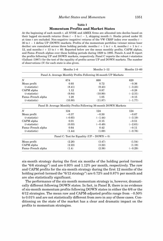
Table IMomentum Profits and Market States

At the beginning of each month t, all NYSE and AMEX firms are allocated into deciles based ontheir lagged six-month returns (from t − 5 to t − 1, skipping month t). Stocks priced under $1at time t are excluded. Non-negative (negative) returns of the VW CRSP index over months t −36 to t − 1 define UP (DOWN) markets. Profits of the momentum portfolios (winner minus loserdeciles) are cumulated across three holding periods: months t + 1 to t + 6, months t + 1 to t +12, and months t + 13 to t + 60. Reported below are the mean monthly profits, CAPM alphas,and Fama–French alphas over these holding periods during 1929 to 1995. Panels A and B reportthe profits following UP and DOWN markets, respectively. Panel C reports the robust t-statistics(Gallant (1987)) for the test of the equality of profits across UP and DOWN markets. The numberof observations (N) for each state is also given.

Months 1–6 Months 1–12 Months 13–60

Panel A: Average Monthly Profits Following 36-month UP Markets

N 674 668 620Mean profit 0.93 0.72 −0.36

(t-statistic) (8.41) (9.43) (−3.23)CAPM alpha 1.12 0.87 −0.28

(t-statistic) (9.84) (10.90) (−2.31)Fama–French alpha 1.28 1.05 −0.15

(t-statistic) (10.80) (11.87) (−1.77)

Panel B: Average Monthly Profits Following 36-month DOWN Markets

N 124 124 124Mean profit −0.37 −0.50 −0.67

(t-statistic) (–0.65) (−1.44) (−3.19)CAPM alpha 0.01 −0.15 −0.51

(t-statistic) (0.03) (−0.49) (−2.61)Fama–French alpha 0.64 0.42 −0.11

(t-statistic) (1.44) (1.69) (−0.76)

Panel C: Test for Equality (UP – DOWN = 0)

Mean profit (2.26) (3.47) (1.54)CAPM alpha (2.22) (3.22) (1.19)Fama–French alpha (1.4) (2.36) (−0.29)

six-month strategy during the first six months of the holding period (termedthe “6/6 strategy”) and are 0.93% and 1.12% per month, respectively. The rawand CAPM profits for the six-month strategy during the first 12 months of theholding period (termed the “6/12 strategy”) are 0.72% and 0.87% per month andare also statistically significant.

The performance of the six-month momentum strategy is, however, dramati-cally different following DOWN states. In fact, in Panel B, there is no evidenceof six-month momentum profits following DOWN states in either the 6/6 or the6/12 strategies. The mean raw and CAPM-adjusted profits range from −0.50%to 0.01% and are not statistically different from zero in any of these cases. Con-ditioning on the state of the market has a clear and dramatic impact on theprofits to momentum strategies.

1352 The Journal of Finance

In Panel C, we provide the t-statistics for testing the equality of the profitsacross UP and DOWN states for the three holding periods. Momentum profitsare statistically greater following UP markets using both the raw and CAPM-adjusted profits for the 6/6 and 6/12 strategy. So, momentum profits are greaterin the short-run following UP markets than following DOWN markets, as pre-dicted by the overreaction theories.

Note also in Table I that there is less evidence that momentum profits aregreater following UP markets than DOWN markets when using the Fama–French model. The differences are only significant for the 6/12 strategy. But wefind in Section II.B that defining the state of the market with lagged two-yearor one-year market returns provides strong evidence that UP-market momen-tum is greater than DOWN-market momentum for the 6/6 strategy even whenusing the three-factor model. The asymmetry in short-run momentum profitsis robust to Fama–French (FF) alphas.

C. The Long-Run Reversal in the Profits to Momentum Strategies

If the short-run momentum profits are an overreaction to news, then we ex-pect to see long-run reversal of the profits to the six-month strategy as themarket eventually corrects the mispricings. Lee and Swaminathan (2000) andJegadeesh and Titman (2001) examine the unconditional mean profits to thesix-month momentum strategy over a five-year holding period and find thatthe profits reverse in years two to five—consistent with overreaction and cor-rection. Figures 1 and 2 plot the cumulative raw and CAPM profits, respec-tively, to the six-month momentum strategy following UP and DOWN statesin holding-period months 1 to 60. The UP-market plots of the raw and CAPMprofits are consistent with the unconditional findings of Lee and Swaminathan

-40%

-30%

-20%

-10%

0%

10%

20%

1 11 21 31 41 51

Holding Period Returns

Cu

mu

lati

ve P

rofi

ts

Raw - UP Raw - DOWN

Figure 1. Cumulative raw profits in UP and DOWN states. The cumulative mean monthlyprofits over the months t + 1 to t + 60 are plotted for the six-month momentum strategy from1929:01 to 1995:12 following three-year UP markets and three-year DOWN markets, respectively.

Market States and Momentum 1353

-40%

-30%

-20%

-10%

0%

10%

20%

1 11 21 31 41 51

Holding Period Returns

Cu

mu

lati

ve P

rofi

ts

CAPM - UP CAPM - DOWN

Figure 2. Cumulative CAPM profits in UP and DOWN states. The cumulative CAPM alphasover the months t + 1 to t + 60 are plotted for the six-month momentum strategy from 1929:01 to1995:12 following three-year UP markets and three-year DOWN markets, respectively.

and Jegadeesh and Titman in that the early momentum profits are offset bysubsequent long-run reversal.

The last column of Table I provides a formal test of the significance of the long-run reversal in the profits. Following UP markets, there is significant evidenceof reversal in the six-month strategy’s profits in months 13 to 60; both the rawand CAPM-adjusted profits are reliably negative. Again, this is consistent withan initial overreaction and subsequent correction.

As discussed earlier, the FF alphas are expected to display less evidence oflong-run reversal. Figure 3 shows this to be the case. But we still can reject inTable I the null hypothesis of zero abnormal returns in the long-run followingUP markets even using the FF method, with a t-statistic of −1.77.

Figures 1 and 2 also indicate that the overreaction theory does not capturethe entire long-run anomaly however. We see strong long-run reversal in theraw and in the CAPM-adjusted profits of the six-month strategy, despite therebeing no early momentum. The average raw and CAPM-adjusted profits duringmonths 13 to 60 in DOWN states are significantly negative at –0.67% and–0.52%, respectively. Long-run reversal can apparently exist without short-run momentum. While overreaction cannot completely explain the short-runmomentum and long-run reversal phenomena, overreaction does seem capableof explaining a large portion of the lagged-return anomalies.

II. Robustness and Other Considerations

A. Can a Macroeconomic Factor Model Explain These Patterns?

Chordia and Shivakumar (2002; hereafter CS) show that commonly-usedmacroeconomic instruments for measuring market conditions can explain a

1354 The Journal of Finance

-40%

-30%

-20%

-10%

0%

10%

20%

1 11 21 31 41 51

Holding Period Returns

Cu

mu

lati

ve P

rofi

ts

FF - UP FF - DOWN

Figure 3. Cumulative Fama–French profits in UP and DOWN states. The cumulativeFama–French three-factor alphas over the months t + 1 to t + 60 are plotted for the six-month mo-mentum strategy from 1929:01 to 1995:12 following three-year UP markets and three-year DOWNmarkets, respectively.

large portion of six-month momentum profits. CS show that, after controllingfor cross-sectional differences in returns predicted using lagged macroeconomicvariables, the portfolios of past winners and past losers do not exhibit short-term return momentum. They conclude that the profitability of momentumstrategies can be attributed to variations in the macroeconomic factors (andpresumably to risk). We examine if such a macroeconomic model can capturethe asymmetries that we find in the profits to the six-month momentum strat-egy. In other words, is the lagged market return a proxy for changes in themacroeconomic variables considered by CS?

The return-generating model that CS employ is

rt = a + b1DIVt−1 + b2DEFt−1 + b3TERMt−1 + b4YLDt−1 + et , (3)

where rt is the return of stock i in month t, a and bk (k = 1, . . . , 4) are coefficients,et is the error term, DIVt−1 is the lagged dividend yield of the CRSP value-weighted index, DEFt−1 is the lagged yield spread between Baa-rated bondsand Aaa-rated bonds, TERMt−1 is the lagged yield spread between ten-yearTreasury bonds and six-month Treasury bills, and YLDt−1 is the lagged yieldon a T-bill with three months to maturity.10

To see the extent to which the macroeconomic multifactor model can explainthe profits of the momentum strategies, we employ two-way dependent sortsas CS do. We first sort all stocks each month into quintiles based on theirpredicted returns from the factor model, and then we sort each of these quintiles

10 We thank Jeff Pontiff for providing the macroeconomic data used by Pontiff and Schall (1998).

Market States and Momentum 1355

further (into quintiles) based on the lagged six-month returns of the stocks. Thepredicted returns from the factor model are calculated as follows.

The loadings for each stock on the four macroeconomic factors are calculatedwith a time-series regression of stock returns on the four factors and an inter-cept using months t − 59 to t. The loadings are updated monthly. We require thateach stock have a minimum of 12 observations within the 60-month window.We calculate the monthly predicted returns (fitted values from the model usinglagged factor realizations and coefficient estimates) for all stocks and compoundthese predictions into a six-month factor-model predicted return from t + 1 tot + 6. Stocks are then sorted into quintiles based on their six-month predictedreturns, and each of these quintiles is further sorted into quintiles based onlagged six-month returns (t − 5 to t − 1, skipping month t). The raw monthlyreturns to each of the 25 portfolios are cumulated over months t + 1 to t + 6 toform CARs as before and are separated into three-year UP and DOWN marketsat time t. The mean profits to these 25 portfolios are calculated and reportedfor each state. Finally, the mean profits to a strategy that buys the winnerlagged-return quintile and sells the loser lagged-return quintile within each ofthe predicted-return quintiles is also reported.

Unlike CS, who sort on formation-period predicted returns, we first sorton predicted returns constructed using realized factor values from the hold-ing period. We contend that the latter window is more appropriate in deter-mining whether the macroeconomic model explains the return patterns (andshould yield a test with greater power). This is analogous to employing the re-alized market return to determine if the CAPM explains a given stock’s returnbehavior.

With these two-way sorts, we can examine if the cross-sectional variationin returns predicted by the macroeconomic factor model captures conditionalvariation in the momentum profits. In Table II, we present the mean profits forthe two-way sorts from 1929 to 1995. Panel A shows that the macroeconomicmodel has no ability to explain the momentum profits following UP states. Thelevel of the momentum profits within each quintile of the factor-model predictedreturns is at least 0.50% per month, and all mean profits are significantlydifferent from zero. As expected, following DOWN states, Panel B shows noevidence of momentum within the predicted-return quintiles. In contrast toCS, the macroeconomic model shows little, if any, ability to capture momentumprofits.

To understand what drives the difference between our findings and thoseof CS, we first replicate their method (on unconditional profits). Using (1) the1963:07 to 1994:12 data, (2) with formation-period predicted returns, (3) withno price screen, (4) without skipping the last month of the six-month lagged-return measure of momentum, and (5) employing the nonoverlapping returnmethod of Jegadeesh and Titman (1993), we are able to reproduce the find-ings of CS reported in Panel B of their Table VII. As shown in Panel A of ourTable III, we also find that the multifactor model captures the unconditionalmomentum profits in the four lowest quintiles of predicted returns. The abilityof the macroeconomic model to capture momentum profits, however, is strongly

1356 The Journal of Finance

Table IITwo-Way Dependent Sorts: Six-Month Factor-Model Predicted

Returns and Then Lagged Six-Month Returns in UP and DOWN StatesAll NYSE and AMEX stocks are first sorted each month t into quintiles based on their six-month(t + 1 to t + 6) predicted returns from the four-factor model: lagged dividend yield of CRSP value-weighted index (DIV), lagged yield spread for Baa bonds over Aaa bonds (DEF), lagged yield spreadfor 10-year Treasury over three-month Treasury (TERM), and lagged yield on a T-bill with threemonths until maturity (YLD). Stocks priced under $1 at time t are excluded. Each predicted-returnquintile is then further sorted into quintiles based on lagged six-month returns (t − 5 to t − 1,skipping month t). Non-negative (negative) returns of the VW CRSP index during months t − 36to t − 1 define UP (DOWN) markets. Returns of the 25 portfolios are cumulated across monthst + 1 to t + 6. In Panel A (B), we report the mean monthly returns following UP (DOWN) marketsfrom 1929 to 1995. The “High-Low” column provides the mean profits of the strategy that buysthe winner quintile and sells the loser quintile within each predicted-return quintile (across eachrow). The robust t-statistics (Gallant (1987)) on the profits to this strategy are given in the lastcolumn. The “ALL” column reports the mean returns in each predicted-return quintile. The numberof observations (N) for each state is also given.

Lagged Six-Month Returns

Macro-Model t-StatPredicted Returns Low 2 3 4 High ALL High-Low (High-Low)

Panel A: Average Monthly Returns Following 36-month UP Markets (N = 674)

Low 0.49 0.80 0.89 1.05 1.14 0.87 0.65 5.892 0.68 0.92 1.01 1.08 1.19 0.98 0.51 6.263 0.78 0.93 1.02 1.09 1.28 1.02 0.50 6.184 0.77 0.96 1.03 1.10 1.32 1.04 0.55 6.64High 0.70 0.97 1.08 1.19 1.31 1.05 0.62 6.51

Panel B: Average Monthly Returns Following 36-month DOWN Markets (N = 124)

Low 3.29 3.15 3.02 2.86 2.77 3.02 −0.51 −1.222 3.25 2.69 2.35 2.30 1.17 2.35 −0.91 −2.203 2.81 2.36 2.06 2.10 2.32 2.33 −0.48 −1.224 2.24 2.10 2.03 1.94 2.30 2.12 0.07 0.17High 2.29 2.29 1.98 2.29 2.85 2.34 0.57 1.37

affected by methodological adjustments commonly used in the momentum liter-ature to mitigate microstructure concerns. Specifically, when we exclude fromthe portfolios stocks priced under $1 at the beginning of the testing period (toeliminate highly illiquid and high-trading-costs stocks) and skip the last monthbetween the formation period and the holding period in constructing the mo-mentum measure (to reduce spurious reversal due to bid–ask bounce), the re-sults change. Jegadeesh and Titman (1993, 2001) and Fama and French (1996),among others, have employed such adjustments to mitigate the microstructureconcerns and thereby better estimate momentum profits. As reported in Panel Bof Table III, the application of these adjustments results in significant momen-tum profits in four of the five quintiles of predicted returns. The predominanteffect of these adjustments is to lower the returns in the lowest quintile of

Market States and Momentum 1357

Table IIITwo-Way Dependent Sorts: Six-Month Factor-Model Predicted

Returns and Then Lagged Six-Month ReturnsAll NYSE and AMEX stocks are first sorted each month t into quintiles based on their six-month(t − 5 to t) predicted returns from the four-factor model: lagged dividend yield of CRSP value-weighted index, lagged yield spread for Baa bonds over Aaa bonds, lagged yield spread for 10-yearTreasury over three-month Treasury, and lagged yield on a T-bill with three months until maturity.In Panel A, each predicted-return quintile is then further sorted into quintiles based on laggedsix-month returns (from t − 5 to t, including month t); no low-price stocks are excluded. Panel Bemploys lagged returns from months t − 5 to t − 1, skipping month t, as the second sort and excludesstocks priced below $1 at time t. We report the mean monthly returns for these 25 portfolios over theholding-period months t + 1 to t + 6 for the period 1963:07 to 1994:12 (the sample period of Chordiaand Shivakumar (2002)). The “High-Low” column provides the mean returns of the strategy thatbuys the winner quintile and sells the loser quintile within each predicted-return quintile (acrosseach row). This table employs the nonoverlapping-return method used by Chordia and Shivakumar(2002). The “ALL” column reports the mean monthly returns in each predicted-return quintile.

Lagged Six-Month Returns

Macro-Model t-StatPredicted Returns Low 2 3 4 High ALL High-Low (High-Low)

Panel A: Average Monthly Returns(formation-period predicted returns, no price screen, not skipping month t)

Low 0.90 0.97 1.05 1.08 1.10 1.02 0.20 0.632 1.08 1.18 1.09 1.14 1.26 1.15 0.18 0.963 1.16 1.25 1.26 1.25 1.30 1.24 0.14 0.804 1.35 1.41 1.46 1.43 1.59 1.45 0.25 1.39High 1.36 1.47 1.54 1.65 1.82 1.57 0.46 2.28

Panel B: Average Monthly Returns(formation-period predicted returns, $1 price screen, skipping month t)

Low 0.23 0.91 1.01 1.08 1.18 0.88 0.95 4.342 0.93 1.14 1.11 1.13 1.30 1.12 0.37 2.343 1.07 1.22 1.25 1.25 1.33 1.22 0.26 1.624 1.23 1.44 1.46 1.46 1.60 1.44 0.37 2.32High 1.23 1.48 1.56 1.63 1.81 1.54 0.58 3.18

lagged-six-month returns. This is consistent with the adjustments succeedingin reducing spurious negative autocorrelation. Note that applying either theprice screen or the skip-month return in isolation is sufficient to reverse theCS findings. Hence, it seems that, while market conditions are critically impor-tant in determining momentum profits, the macroeconomic-based proxies forthe market’s state are not useful (only the lagged return of the market is).11

11 We also examined several variations of the macroeconomic model, and the results do notchange. We considered the predicted returns (1) without including the intercept, (2) estimatingfactor loadings using a two-year window instead of a five-year one, (3) using portfolio loadings(from 50 size portfolios) as proxies for individual stock loadings, and (4) using a multiple-step-ahead forecast from the macro model to predict holding-period returns using only informationavailable at time t.

1358 The Journal of Finance

0

2

4

6

8

10

12

1930 1935 1940 1945 1950 1955 1960 1965 1970 1975 1980 1985 1990 1995

Year

Nu

mb

er o

f D

OW

N m

on

ths

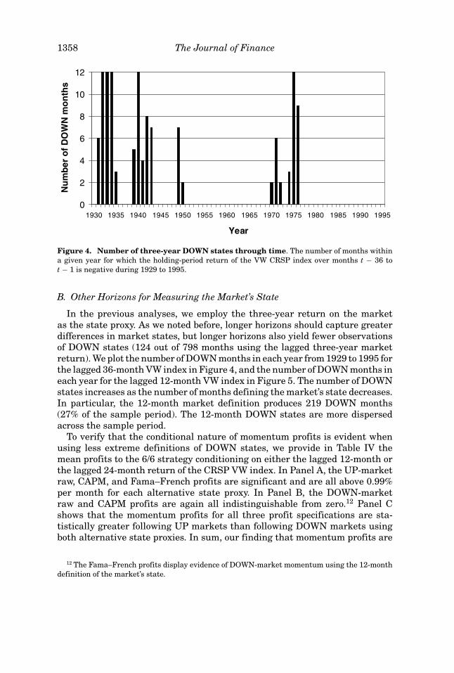
Figure 4. Number of three-year DOWN states through time. The number of months withina given year for which the holding-period return of the VW CRSP index over months t − 36 tot − 1 is negative during 1929 to 1995.

B. Other Horizons for Measuring the Market’s State

In the previous analyses, we employ the three-year return on the marketas the state proxy. As we noted before, longer horizons should capture greaterdifferences in market states, but longer horizons also yield fewer observationsof DOWN states (124 out of 798 months using the lagged three-year marketreturn). We plot the number of DOWN months in each year from 1929 to 1995 forthe lagged 36-month VW index in Figure 4, and the number of DOWN months ineach year for the lagged 12-month VW index in Figure 5. The number of DOWNstates increases as the number of months defining the market’s state decreases.In particular, the 12-month market definition produces 219 DOWN months(27% of the sample period). The 12-month DOWN states are more dispersedacross the sample period.

To verify that the conditional nature of momentum profits is evident whenusing less extreme definitions of DOWN states, we provide in Table IV themean profits to the 6/6 strategy conditioning on either the lagged 12-month orthe lagged 24-month return of the CRSP VW index. In Panel A, the UP-marketraw, CAPM, and Fama–French profits are significant and are all above 0.99%per month for each alternative state proxy. In Panel B, the DOWN-marketraw and CAPM profits are again all indistinguishable from zero.12 Panel Cshows that the momentum profits for all three profit specifications are sta-tistically greater following UP markets than following DOWN markets usingboth alternative state proxies. In sum, our finding that momentum profits are

12 The Fama–French profits display evidence of DOWN-market momentum using the 12-monthdefinition of the market’s state.

Market States and Momentum 1359

0

2

4

6

8

10

12

1930 1935 1940 1945 1950 1955 1960 1965 1970 1975 1980 1985 1990 1995

Year

Nu

mb

er o

f D

OW

N m

on

ths

Figure 5. Number of one-year DOWN states through time. The number of months within agiven year for which the holding-period return of the VW CRSP index over months t − 12 to t − 1is negative during 1929 to 1995.

critically dependent on the state of the market is robust to using lagged two-year or lagged one-year market returns as the proxy for the market’s state.

C. The Market’s State as a Continuous Variable

We also examine the relation between the lagged market return and momen-tum profits using the market’s return as a continuous variable, not just thediscrete UP and DOWN states as before. In particular, we are interested if mo-mentum profits increase monotonically with the lagged market return. Whenthe lagged market return is highest, are momentum profits the greatest?

To determine this, we regress momentum profits on lagged market returnsas well as the square of lagged market returns. We report the results usingthe lagged 36-month market return as the state proxy (the 12-month and24-month results are similar). As shown in Panel A of Table V, the raw andrisk-adjusted profits are positively related to lagged market returns, confirm-ing our finding that momentum is high (low) when lagged market return is high(low). Interestingly, the profits are negatively related to the square of laggedmarket returns, indicating that profits do not increase linearly with laggedmarket returns.13 In Panel B, we report the momentum profits ranking themarket’s 36-month lagged returns into quintiles. We see that profits increase

13 Jegadeesh and Titman (1993) also examine the relation between momentum profits and thesquare of the lagged market return. However, since their intent is to examine if lead-lag effects area source of momentum profits, they employ the lagged market return over the six-month formationperiod of the momentum portfolios. They find a negative coefficient on the squared market returnand conclude that this is inconsistent with lead-lag effects contributing to momentum profits.

1360 The Journal of Finance

Table IVMomentum Profits and Alternative Definitions of Market States

At the beginning of each month t, all NYSE and AMEX firms are allocated into deciles based ontheir lagged-six-month returns (from t − 5 to t − 1, skipping month t). Stocks priced under $1 at timet are excluded. Returns on the VW CRSP index are computed over the period t − m to t − 1 (wherem = 12 or 24), and non-negative (negative) returns of the VW CRSP index define UP (DOWN)markets. Profits of the momentum portfolios (winner minus loser deciles) are cumulated acrossmonths t + 1 to t + 6. Reported below are the mean monthly profits, CAPM alphas, and Fama–French alphas. The sample period is from 1929 to 1995. Panels A and B report the profits followingUP and DOWN markets, respectively. Panel C reports the robust t-statistics (Gallant (1987)) forthe test of the equality of profits across UP and DOWN markets. The number of observations (N)for each state is also given.

12-Month Market 24-Month Market

Panel A: Average Monthly Profits Following UP Markets

N 579 667Mean profit 1.04 0.99

(t-statistic) (9.23) (9.53)CAPM alpha 1.22 1.18

(t-statistic) (10.42) (10.88)Fama–French alpha 1.37 1.32

(t-statistic) (11.01) (11.71)

Panel B: Average Monthly Profits Following DOWN Markets

N 219 131Mean profit −0.08 −0.55

(t-statistic) (–0.22) (−0.99)CAPM alpha 0.22 −0.21

(t-statistic) (0.72) (−0.45)Fama–French alpha 0.68 0.43

(t-statistic) (2.42) (1.01)

Panel C: Test for Equality (UP − DOWN = 0)

Mean profit (3.00) (2.27)CAPM alpha (3.05) (2.93)Fama–French alpha (2.28) (2.05)

dramatically from the lowest levels of lagged market returns to quintile 2. Prof-its continue to increase as the market state improves, but peak at the medianlevels of lagged market return. It is important to point out that momentumprofits remain significant even at the highest levels of the market’s state.

The nonlinear relation documented in Table V seems to suggest that over-reactions may actually be diminishing beyond some threshold level of priormarket performance. We offer two potential explanations of this phenomenon.First, it might be that the extreme levels of the market’s performance are co-incident with the ending of the overreaction phase and the beginning of thecorrectional reversals, triggered by the arrival of fundamental news. The on-set of the reversals would of course diminish the momentum profits. Second, it

Market States and Momentum 1361

Table VThe Lagged Market Return as a Continuous Measure of the State

of the MarketAt the beginning of each month t, all NYSE and AMEX firms are allocated into deciles based on theirlagged-six-month returns (month t − 5 to month t − 1, skipping month t). Profits on the momentumportfolios (winner minus loser deciles) are cumulated across months t + 1 to t + 6. The six-monthcumulative profits (raw, CAPM-adjusted, and Fama–French three-factor-adjusted) are regressedon an intercept, lagged 36-month market return (LAGMKT), and lagged 36-month market returnsquared (LAGMKT2). Panel A provides the monthly regression coefficients and robust t-statistics(Gallant (1987)). In Panel B, momentum portfolios are allocated each month t into quintiles based onthe full sample of lagged 36-month market returns; mean monthly momentum profits are reportedalong with their robust t-statistics.

Panel A: 36-month Lagged Market

Intercept LAGMKT LAGMKT2 Adj-R2

Mean profit 0.39 2.77 −2.40 0.10(t-statistic) (1.30) (2.41) (−2.60)

CAPM alpha 0.69 2.33 −2.12 0.08(t-statistic) (2.83) (2.38) (−2.65)

Fama–French alpha 1.07 1.34 −1.33 0.03(t-statistic) (4.70) (1.62) (−2.06)

Panel B: Momentum Profits by Quintiles of Lagged 36-month Market States

Low 2 3 4 High

Mean profit −0.12 0.94 1.30 0.92 0.61(t-statistic) (−0.27) (3.58) (8.31) (5.78) (3.14)

CAPM alpha 0.17 1.22 1.50 1.19 0.64(t-statistic) (0.43) (4.80) (8.76) (7.06) (3.05)

Fama–French alpha 0.73 1.25 1.66 1.48 0.77(t-statistic) (1.97) (4.61) (10.12) (8.38) (3.69)

might be that investors are acquiring less private information in the extremegood states (to overreact to). Welch (2000) finds evidence consistent with thisin his study of analyst herding. There is more herding when prior returns arehighest indicating that there is less unique information in good times.14

D. The Lagged Market Return versus the MacroeconomicVariables as Time-Series Predictors

In Section II.A, we found that the macroeconomic factor model does not ro-bustly capture the cross-sectional differences in returns between prior winnerstocks and prior loser stocks. In this section, we consider whether the laggedmarket return is a better time-series predictor of momentum profits than the

14 Note also that overconfidence theory does not necessarily predict a fully monotonic relationbetween lagged market returns and the level of overconfidence. As Gervais and Odean (2001)pointed out, overconfident investors might learn of their bias over time.

1362 The Journal of Finance

popular macroeconomic factors used in equation (3). We do this by examiningthe recursive out-of-sample forecasts of momentum profits formed from thetwo competing sets of information: (1) lagged market returns, and (2) macroe-conomic variables. The out-of-sample analysis complements the prior evidenceon the robustness of the relation between momentum profits and the state ofthe market.

To simplify the out-of-sample procedure and maintain a “real-time” frame-work, the momentum profit series that we seek to predict is the mean profit incalendar month τ across the six momentum portfolios that are “open” in cal-endar month τ (Jegadeesh and Titman (1993)). The first momentum portfoliois in holding-period month one during month τ , and the sixth portfolio is inholding-period month six during month τ . Two out-of-sample forecasts for thistimes-series of momentum profits are obtained each month as follows.

The first forecast is estimated using the lagged market return and the squareof the lagged market return. The second forecast is estimated using the fourmacroeconomic variables in equation (3), DIVt−1, DEFt−1, TERMt−1, andYLDt−1. The loadings of the momentum profits on each set of “factors” areestimated with a time-series regression of momentum profits on each separateset of factors and an intercept using calendar months τ − 120 to τ − 1 for thefirst forecast in January 1939. The loadings are updated monthly. We start withan initial in-sample period of 10 years, and then allow the in-sample window toexpand each month as we roll through the sample. We form the predicted prof-its each month using the estimated loadings from the most recent in-sampleregression and the lagged factor realizations.

The “lagged-market” forecasts and the “macro” forecasts are evaluated us-ing two methods. For the first method, we regress the time-series of momen-tum profits on the two time-series of out-of-sample forecasts and a constant.The t-statistics on the slope coefficients test that the forecasts provide infor-mation about momentum profits. The second method is to compare the meanabsolute errors of each forecast (MAE) to the mean absolute error of the “un-conditional” forecast, which is the historical mean monthly momentum profitfrom the rolling in-sample windows. Finding that the MAE of the forecasts issmaller than the unconditional MAE is evidence of the extent to which momen-tum profits are forecastable using either the lagged-market variables or themacro variables.

As we do in the prior analyses, we examine raw, CAPM-adjusted, and Fama–French-adjusted profits (see equation (1) for our method of adjustment). Theout-of-sample results are reported in Table VI. They clearly show that thelagged market return alone possesses the ability to predict time-series vari-ations in momentum profits. The t-statistics from the regressions of momen-tum profits on the forecasts are above 2.0 for the lagged-market forecasts inall three measures of the profit series. The t-statistics for the macro forecastsare small, and the coefficients are even the wrong sign. In addition, the MAEof the lagged-market forecasts is statistically smaller than the MAE of the un-conditional forecast at the 5% level or lower in all three of the profit series(using the z-statistics suggested by Diebold and Mariano (1995)). In fact, the

Market States and Momentum 1363

Table VIThe Forecasting Abilities of the Lagged Market Return

versus the Macroeconomic VariablesAt the beginning of each month t, all NYSE and AMEX firms are allocated into deciles based on theirlagged six-month returns (month t − 5 to month t − 1, skipping month t). In a given calendar monthτ , the profits to the six “open” momentum portfolios (winner minus loser deciles) are calculated. Acalendar time-series of momentum profits is formed from the mean profits across the six portfoliosin month τ . The raw, CAPM-adjusted, and Fama–French three-factor adjusted monthly profits areregressed on an intercept, lagged 36-month market return, and the square of the lagged 36-monthmarket return using an in-sample window of 10 years ending December 1938. The forecasted valuesfor January 1939 from this “lagged market” model are formed. The in-sample window is expandedone month, and the forecasted momentum profits for February 1939 are formed, and so on. A time-series of out-of-sample forecasts using the four macroeconomic variables, DIV, TERM, DEF, andYLD is formed similarly and is termed the “macro variables” model (see Table II for definitions ofthese variables). The “unconditional” forecasts are the rolling historical mean of the profit series.Momentum profits from 1939:01 to 1995:12 are regressed onto their forecasted values from thelagged-market model and the macro variables model in a multiple regression. The t-statistics ofthe slope coefficients for each forecast are given below. The mean absolute forecast error for eachmodel is also given.

Forecast Type t-Statistic Mean Absolute Error

Mean profit Unconditional −0.32 2.95Lagged market 2.04 2.87∗∗∗Macro variables −0.79 3.06∗

CAPM alpha Unconditional −0.78 3.20Lagged market 2.06 3.13∗∗∗Macro variables −1.22 3.26

Fama–French alpha Unconditional −1.48 2.94Lagged market 2.37 2.91∗∗Macro variables −1.72 2.96

Note: The symbols ∗∗∗, ∗∗, and ∗ indicate that the mean absolute error is statistically different thanthe mean absolute error of the unconditional model at the 1%, 5%, and 10% significance levels,respectively (using the z-statistic of Diebold and Mariano (1995)).

lagged-market forecasts outperform the unconditional historical mean by about60 to 96 basis points per year. The MAE for the macro forecasts though is on av-erage greater than the unconditional MAE in all cases, and is statistically worsethan the unconditional MAE for the mean profit series. In sum, the lagged mar-ket return provides robust information about future momentum profits whilethe macro variables display no reliable information.15

III. Conclusion

We find that the profits to momentum strategies depend critically on thestate of the market. A six-month momentum portfolio is profitable only

15 The out-of-sample results for the macro variables are consistent with the findings in Table IV ofChordia and Shivakumar (2002) that the loadings of the momentum portfolio on the macroeconomicvariables are nonstationary over time, even changing signs in some cases across subperiods. Weconfirm this finding of nonstationarily in the macro factor loadings.

1364 The Journal of Finance

following periods of market gains (UP market states), consistent with the over-reaction models of Daniel et al. (1998) and Hong and Stein (1999). We find thatmomentum profits increase as the lagged market return increases. However,at high levels of lagged market returns, the profits diminish but are not elimi-nated. Additionally, we reconfirm the findings of Lee and Swaminathan (2000)and Jegadeesh and Titman (2001) that momentum profits are reversed in thelong-run, as predicted by the overreaction theories. We also find significantlong-run reversal in the DOWN states although there is no initial momentum.This finding indicates that long-run reversal is not solely due to the correctionsof prior momentum.

A multifactor macroeconomic model of returns, as used by Chordia andShivakumar (2002), does not explain momentum profits. We find that the abilityof such a model to explain momentum profits is not robust to controls for marketfrictions (specifically, a price screen and skip-month returns). Additionally, wefind that the macroeconomic model cannot forecast the time-series of momen-tum profits out-of-sample, while the lagged return of the market can. Hence,we identify that the lagged return of the market is the type of conditioninginformation that is relevant for predicting the profitability of the momentumstrategies.

Overall, our findings of asymmetries conditional on the state of the marketcomplements the evidence of asymmetries in factor sensitivities, volatility, cor-relations, and expected returns found by Boudoukh, Richardson, and Whitelaw(1997), Whitelaw (2000), Perez-Quiros and Timmermann (2000), and Ang andChen (2002). These studies indicate that models of asset pricing, both rationaland behavioral, need to incorporate (or predict) such regime switches.

REFERENCESAhn, Dong H., Jennifer Conrad, and Robert F. Dittmar, 2002, Risk adjustment and trading strate-

gies, Review of Financial Studies 16, 459–485.Ang, Andrew, and Joseph Chen, 2002, Asymmetric correlations of equity portfolios, Journal of

Financial Economics 63, 443–494.Barberis, Nicholas, Ming Huang, and Tanos Santos, 2001, Prospect theory and asset prices, Quar-

terly Journal of Economics 116, 1–53.Barberis, Nicholas, Andrei Shleifer, and Robert Vishny, 1998, A model of investor sentiment, Jour-

nal of Financial Economics 49, 307–343.Boudoukh, Jacob, Matthew Richardson, and Robert F. Whitelaw, 1997, Nonlinearities in the re-

lation between the equity risk premium and the term structure, Management Science 43,371–385.

Campbell, John Y., and John H. Cochrane, 1999, By force of habit: A consumption-based explanationof aggregate stock market behavior, Journal of Political Economy 107, 205–251.

Chordia, Tarun, and Lakshmanan Shivakumar, 2002, Momentum, business cycle and time-varyingexpected returns, Journal of Finance 57, 985–1019.

Cooper, Michael, 1999, Filter rules based on price and volume in individual security overreaction,Review of Financial Studies 12, 901–935.

Daniel, Kent, David Hirshleifer, and Avanidhar Subrahmanyam, 1998, Investor psychology andinvestor security market under-and overreactions, Journal of Finance 53, 1839–1886.

Daniel, Kent, David Hirshleifer, and Siew Hong Teoh, 2002, Investor psychology in capital markets:Evidence and policy implications, Journal of Monetary Economics 49, 139–209.

Market States and Momentum 1365

Daniel, Kent, and Sheridan Titman, 1997, Evidence on the characteristics of cross sectional vari-ation in stock returns, Journal of Finance 52, 1–33.

DeBondt, Werner F. M., and Richard Thaler, 1985, Does the stock market overreact? Journal ofFinance 40, 793–808.

Diebold, Francis X., and Roberto S. Mariano, 1995, Comparing predictive accuracy, Journal ofBusiness and Economic Statistics 13, 253–263.

Fama, Eugene F., and Kenneth R. French, 1993, Common risk factors in the returns on stocks andbonds, Journal of Financial Economics 33, 3–56.

Fama, Eugene F., and Kenneth R. French, 1996, Multifactor explanations of asset pricing anoma-lies, Journal of Finance 51, 55–84.

Gallant, A. Ronald, 1987, Nonlinear Statistical Models (Wiley, New York).Gervais, Simon, and Terrance Odean, 2001, Learning to be overconfident, Review of Financial

Studies 14, 1–27.Ghysels, Eric, 1998, On stable factor structures in the pricing of risk: Do time-varying betas help

or hurt? Journal of Finance 53, 549–573.Griffin, John M., Susan Ji, and J. Spencer Martin, 2003, Momentum investing and business cycle

risk: Evidence from pole to pole, Journal of Finance 58, 2515–2547.Grinblatt, Mark, and Tobias J. Moskowitz, 2003, Predicting stock price movements from past

returns: The role of consistency and tax-loss selling, Journal of Financial Economics(forthcoming).

Hirshleifer, David, 2001, Investor psychology and asset pricing, Journal of Finance 56, 1533–1597.Holden, Craig W., and Avanidhar Subrahmanyam, 2002, News, events, information acquisition,

and serial correlation, Journal of Business 75, 1–32.Hong, Hong, and Jeremy Stein, 1999, A unified theory of underreaction, momentum trading, and

overreaction in asset markets, Journal of Finance 54, 2143–2184.Jegadeesh, Narasimhan, and Sheridan Titman, 1993, Returns to buying winners and selling losers:

Implications for stock market efficiency, Journal of Finance 48, 65–91.Jegadeesh, Narasimhan, and Sheridan Titman, 2001, Profitability of momentum strategies: An

evaluation of alternative explanations, Journal of Finance 56, 699–720.Korajczyk, Robert, and Ronnie Sadka, 2002, Are momentum profits robust to trading costs? Journal

of Finance 59, 1039–1082.Lakonishok, Josef, Andrei Shleifer, and Robert W. Vishny, 1994, Contrarian investment, extrapo-

lation, and risk, Journal of Finance 49, 1541–1578.Lee, Charles M. C., and Bhaskaran Swaminathan, 2000, Price momentum and trading volume,

Journal of Finance 55, 2017–2069.Lehmann, Bruce, 1990, Fads, martingales, and market efficiency, Quarterly Journal of Economics

105, 1–28.Lesmond, David A., Michael J. Schill, and Chunsheng Zhou, 2002, The illusory nature of momentum

profits, Journal of Financial Economics 71, 349–380.Lo, Andrew W., and A. Craig MacKinlay, 1990, When are contrarian profits due to stock market

overeaction? Review of Financial Studies 3, 175–206.Nagel, Stefan, 2001, Is it overreaction: The performance of value and momentum strategies at long

horizons, Working paper, London Business School.Perez-Quiros, Gabriel, and Allan Timmermann, 2000, Firm size and cyclical variations in stock

returns, Journal of Finance 55, 1229–1262.Pontiff, Jeffrey, and Lawrence D. Schall, 1998, Book-to-market ratios as predictors of market re-

turns, Journal of Financial Economics 49, 141–160.Rouwenhorst, K. Geert, 1998, International momentum strategies, Journal of Finance 53, 267–284.Welch, Ivo, 2000, Herding among security analysts, Journal of Financial Economics 58, 369–396.Whitelaw, Robert F., 2000, Stock market risk and return: An equilibrium approach, Review of

Financial Studies 13, 521–547.Yao, Tong, 2002, Systematic momentum, Working paper, University of Arizona.

1366