MARKETING AND CROP INSURANCE COMBINED TO MANAGE RISK ON A
CASS COUNTY REPRESENTATIVE FARM
A Paper Submitted to the Graduate Faculty
of the North Dakota State University
of Agriculture and Applied Science
By
Aaron D. Clow
In Partial Fulfillment of the Requirements for the Degree of
MASTER OF SCIENCE
Major Department: Agribusiness and Applied Economics
July 2001
Fargo, North Dakota
ii
North Dakota State University Graduate School
Title
MARKETING AND CROP INSURANCE COMBINED TO MANAGE RISK ________ ON A CASS COUNTY REPRESENTATIVE FARM__ _____
By
_______________ __Aaron D. Clow_______________________
The Supervisory Committee certifies that this disquisition complies with North Dakota State University’s regulations and meets the accepted standards
for the degree of
__________________MASTER OF SCIENCE____________________
SUPERVISORY COMMITTEE: ___________________________________________________________
___________________________________________________________
___________________________________________________________
___________________________________________________________
Approved by Department Chair: _______________ ________________________________________ Date
Signature
iii
ABSTRACT
Clow, Aaron D., M.S., Department of Agribusiness and Applied Economics, College of Agriculture, North Dakota State University, July 1996. Marketing and Crop Insurance Combined to Manage Risk on a Cass County Representative Farm. Major Professor: George K. Flaskerud.
This study analyzed the effects that the use of crop insurance products and
marketing alternatives had on the gross revenue per acre for an individual farm in Cass
County. Crop insurance products and marketing strategies were analyzed individually to
determine if they were effective in minimizing down side risk and combined to determine
if integration created synergies. An entire whole farm scenario analysis was run that
included integrated strategies that implemented the same insurance coverage and marketing
alternatives for each crop.
Several general conclusions can be drawn for situations similar to the representative
farm. When analyzed at the individual crop level, the use of crop insurance at the 65
percent level minimizes down side risk in wheat and corn, but not significantly in
soybeans. Marketing alternatives generally increase the up side potential of gross revenue
per acre while doing little to minimize the down side risk.
The integration of crop insurance products and marketing alternatives creates a
synergy at the lower levels of value at risk, where the down side risk is located. However,
the use of integrated strategies does not increase the chances of achieving a cash flow
breakeven gross revenue per acre over the base strategy, which did not include insurance
or marketing alternatives. The breakeven level is not reached until the 70 percent level,
which means that, 7 out of 10 years, the farm will not cash flow. Output from the Bullock
and AgRisk models is similar.
iv
ACKNOWLEDGMENTS
My great appreciation goes to the following people who assisted and supported me
in my pursuit of a master’s degree in Agricultural Economics: my adviser, George
Flaskerud, who went the extra mile for me; Shelly Swandal who put all the finishing
touches on my thesis; David Lambert and the support of the Agribusiness and Applied
Economics Department; the graduate committee for approving my graduate work; and
Mom and Dad for their unconditional love and support.
v
TABLE OF CONTENTS
ABSTRACT..................................................................................................................... iii ACKNOWLEDGMENTS ............................................................................................... iv LIST OF TABLES........................................................................................................... viii
LIST OF FIGURES ......................................................................................................... x CHAPTER 1. INTRODUCTION ................................................................................... 1
Risk Defined ........................................................................................................ 1
Policy Changes .................................................................................................... 2
Government Farm Support Policy ........................................................... 2
International Trade Agreements .............................................................. 3
Currency Fluctuation ............................................................................... 4
Climatic Phenomena ............................................................................................ 4
Need for Study ..................................................................................................... 5
Study Objectives .................................................................................................. 6
Study Area ........................................................................................................... 6
Outline ................................................................................................................. 7
CHAPTER 2. REVIEW OF RISK.................................................................................. 8
Risk Attitudes ...................................................................................................... 8
Ability to Assume Risk........................................................................................ 10
Responses to Price and Yield Risk ...................................................................... 12
Marketing Responses........................................................................................... 13
Elevator Contracts ................................................................................... 14
Futures Market Contracts ........................................................................ 15
vi
Crop Insurance Products ..................................................................................... 16
Catastrophic Coverage............................................................................. 17
Multi-Peril Coverage ............................................................................... 18
Crop Revenue Coverage .......................................................................... 18
Income Protection.................................................................................... 19
Revenue Assurance.................................................................................. 19
Integrated Strategies ............................................................................................ 20
CHAPTER 3. DATA ...................................................................................................... 22
Crops Included..................................................................................................... 22
County, Crop Reporting District, and State Data ................................................ 22
Individual Farm Yield Data ................................................................................. 26
Prices ................................................................................................................. 28
CHAPTER 4. MODELS AND STRATEGIES .............................................................. 32
Bullock Model ..................................................................................................... 32
Farm Information..................................................................................... 32
Crop Distributions ................................................................................... 33
Correlation ............................................................................................... 34
Crop Risk Management Components ...................................................... 34
Crop Risk Management Strategies .......................................................... 35
AgRisk Model...................................................................................................... 36
Farm Information..................................................................................... 36
Market Information.................................................................................. 36
View Results ............................................................................................ 37
vii
Strategies Tested ............................................................................................... 37
CHAPTER 5. RESULTS................................................................................................ 39
Initial Whole Farm Scenario................................................................................ 39
Insurance Products Compared ................................................................. 40
Marketing Alternatives Compared .......................................................... 41
Integrated Strategies Compared............................................................... 44
Sensitivity Analysis ................................................................................. 45
Stochastic Dominance Test...................................................................... 47
Mean-Variance Test................................................................................. 47
Single Crop Scenarios.......................................................................................... 49
Insurance Products Compared ................................................................. 51
Marketing Strategies Compared .............................................................. 51
Secondary Whole Farm Scenario ........................................................................ 52
Strategies Compared................................................................................ 55
Model Comparison .............................................................................................. 55
CHAPTER 6. SUMMARY AND IMPLICATIONS...................................................... 59
Integrated Risk Management Strategy Implications............................................ 60
Model Implications .............................................................................................. 62
Limitation of Study and Suggestions for Further Research................................. 63
REFERENCES ................................................................................................................ 64 APPENDIX A. INITIAL WHOLE FARM SIMULATION OUTPUT.......................... 67 APPENDIX B. SINGLE CROP SIMULATION OUTPUT........................................... 78
viii
LIST OF TABLES Table Page 1. Example Farm Financial Situations: Costs Per Acre........................................... 12 2. Calculation of Acres Planted on a Representative Farm ..................................... 23 3. Cass County Yields (bu/a) Per Planted Acre....................................................... 24 4. Inflated Marketing Year Average Prices ($/bu) 1980-1996................................ 25 5. Price and Yield Correlation ................................................................................. 26 6. Individual Farm Yield (bu/a) Data ...................................................................... 27 7. Insurance Premiums and Base Prices .................................................................. 28 8. Hunter Grain Company Forward Contracting Prices ($/bu)................................ 29 9. Hunter Grain Company 11-Year Historical Average and Standard Deviation of the Basis During Specified Deliver Months (in parentheses) ......................... 29 10. Put Premiums, April 26, 1999 ............................................................................. 30 11. Call Option Premiums, April 26, 1999................................................................ 30 12. Marketing Strategies Used in the Initial Whole Farm Scenario Simulation ....... 38 13. Comparison of Gross Revenue Per Acre of Each Insurance Product and a Base Strategy that Included No Insurance.................................................................... 40 14. Comparison of Gross Revenue Per Acre of Selected Marketing Alternatives with a Base Strategy that Included a Harvest Time Sale of All Production........ 42 15. Comparison of Gross Revenue Per Acre of Individual Strategies with a Integrated Strategy to Check for Synergies ......................................................... 43 16. Gross Revenue Per Acre of Marketing Strategies Combined with the 65 Percent Coverage Level of CRC Insurance ......................................................... 45 17. Gross Revenue Per Acre for Single Crop Analysis of Marketing Strategies with
Wheat and Corn Having CRC Insurance and Soybeans Having CAT Insurance 53
18. Gross Revenue Per Acre of the Four Strategies Tested in the Secondary Whole Farm Simulation .................................................................................................. 54
ix
19. Gross Revenue Per Acre Output Comparison of Bullock and AgRisk Models,
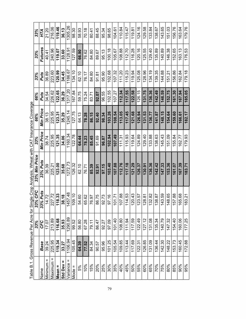
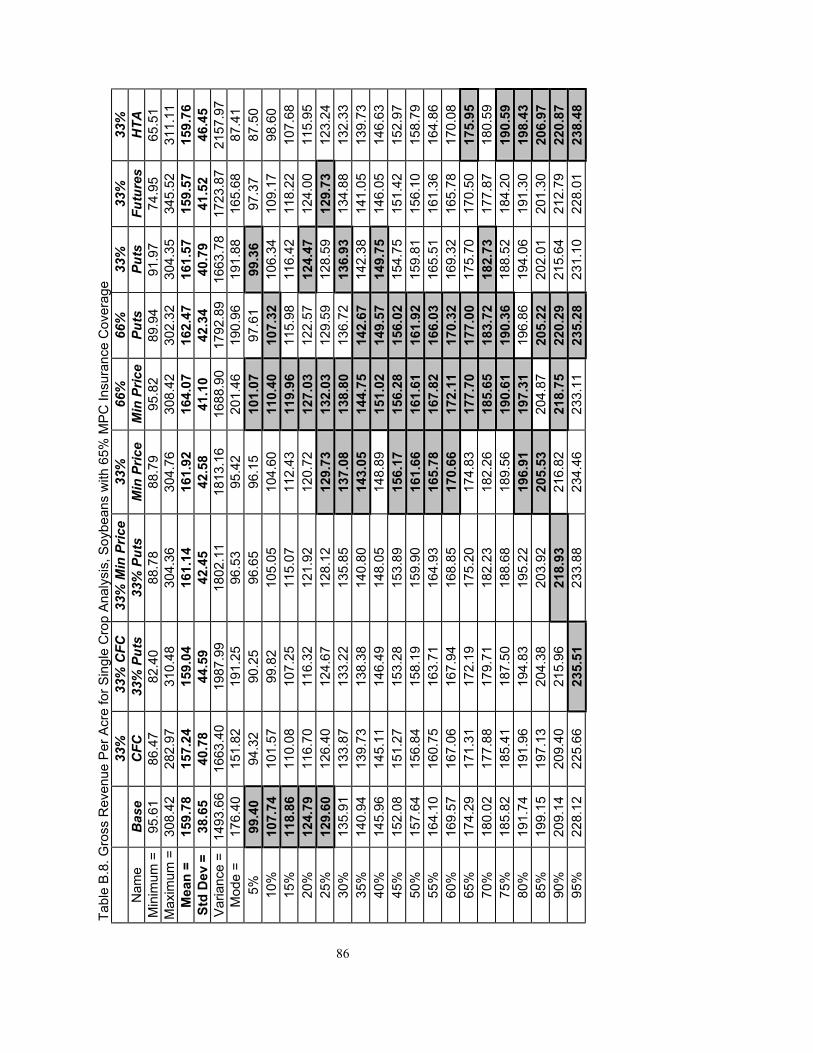
Where the Bullock6 Model is Calculated with and without the Inclusion of an LDP on the Crops ................................................................................................ 57 A.1. Gross Revenue Per Acre for CAT coverage with Selected Marketing Strategies.............................................................................................................. 68 A.2. Gross Revenue Per Acre for 65% MPC Coverage with Selected Marketing Strategies.............................................................................................................. 70 A.3. Gross Revenue Per Acre for 65% CRC Coverage with Selected Marketing Strategies.............................................................................................................. 72 A.4. Gross Revenue Per Acre for 65% RA Coverage with Selected Marketing Strategies.............................................................................................................. 74 A.5. Gross Revenue Per Acre for 65% IP Coverage with Selected Marketing Strategies.............................................................................................................. 76 B.1. Gross Revenue Per Acre for Single Crop Analysis, Wheat with CAT Insurance Coverage ............................................................................................. 79 B.2. Gross Revenue Per Acre for Single Crop Analysis, Wheat with 65% MPC Insurance Coverage ............................................................................................. 80 B.3. Gross Revenue Per Acre for Single Crop Analysis, Wheat with 65% CRC Insurance Coverage ............................................................................................. 81 B.4. Gross Revenue Per Acre for Single Crop Analysis, Corn with CAT Insurance Coverage ............................................................................................. 82 B.5. Gross Revenue Per Acre for Single Crop Analysis, Corn with 65% MPC Insurance Coverage ............................................................................................. 83 B.6. Gross Revenue Per Acre for Single Crop Analysis, Corn with 65% CRC Insurance Coverage ............................................................................................. 84 B.7. Gross Revenue Per Acre for Single Crop Analysis, Soybeans with CAT Insurance Coverage ............................................................................................. 85 B.8. Gross Revenue Per Acre for Single Crop Analysis, Soybeans with 65% MPC Insurance Coverage .................................................................................... 86 B.9. Gross Revenue Per Acre for Single Crop Analysis, Soybeans with 65% CRC Insurance Coverage ............................................................................................. 87
x
LIST OF FIGURES
Figure Page 1. Risk Averse Utility Function ............................................................................... 9 2. Risk Preferring Utility Function .......................................................................... 9 3. Tornado Graph of Sensitivities of the 33 Percent Minimum Price Contracting
Strategy Combined with 65 Percent CRC Coverage ........................................... 46 4. Stochastic Dominance Test of CRC Marketing Strategies.................................. 48 5. Mean-Variance Test of CRC Marketing Strategies............................................. 50
1
CHAPTER 1
INTRODUCTION
Risk management has become increasingly important in farming operations. Over
the past decade, there have been government policy changes, as well as climactic
occurrences, that have led to increased price and yield risk faced by farmers. A 54 percent
decline in median net farm income on farms enrolled in the North Dakota Farm and Ranch
Business Management Education Program from 1993-1998 indicates how farmers in this
state have been adversely affected by increased risk to their operation (Swenson, 1999).
Risk Defined
Risk and uncertainty are often used interchangeably, but the two differ
considerably. According to Knight (1921), risk is faced when the possible outcomes are
known as well as probabilities associated with each. Uncertainty is faced when the possible
outcomes are known, but the probabilities are not. Patrick (1992) defines production risk as
the random variability inherent in a farm’s production process. A few factors that can lead
to this variability are weather, disease, pest infestation, fire, wind, and theft. Price risk
contains three components: basis risk, futures price risk, and futures price spread risk.
Variability in any of these three factors can lead to lower income. Managing risk means
defining the potential range of outcomes, taking steps to reduce the chances of an
unfavorable outcome, and taking actions which will reduce the adverse consequences of an
unfavorable event occurring.
Historical price data are available for most agricultural commodities; therefore, a
probability distribution can be built around the possible values faced in the upcoming crop
year. Probability distribution can also be done with yield data, whether it is actual farm
2
production history or county average yields. Farmers can use this information to manage
the risk of an unfavorable outcome.
Policy Changes
Several policy changes have occurred in the past five years, including a major
change in the government farm support policy as well as several international trade
agreements. The policy changing the government farm support program is called the
Federal Agricultural Improvement Reform (FAIR) Act of 1996, also known as the
“Freedom to Farm” Act. Included in the international trade agreements are the North
American Free Trade Agreement (NAFTA) in 1994, the General Agreement on Trades and
Tariffs (GATT), and the Uruguay Round Agreements of 1994 that established the World
Trade Organization that “replaced GATT as an institutional framework for overseeing
trade negotiations” (USDA, Economic Research Service, 1998). These policies alone have
increased price risk, and according to Wisner, Baldwin, and Blue (1998), they have
“propelled the global agricultural economy into a more market-oriented environment with
reduced government safety nets and less direct involvement of government agencies in
stabilizing grain prices.”
Government Farm Support Policy
There are two major legislative changes in the Freedom to Farm bill. First, the
government will no longer support commodity prices received by farmers through
deficiency payments. Instead, farmers will receive a predetermined “transition” payment
each year until 2002. Second, the supply is no longer controlled by acreage limitations,
formerly called set aside, as well as government controlled release of grain stocks into the
market. These two changes were made in an attempt to produce a more efficient price
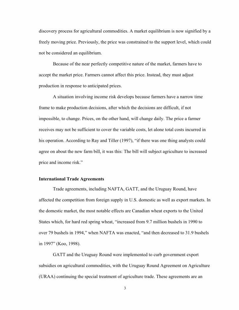
3
discovery process for agricultural commodities. A market equilibrium is now signified by a
freely moving price. Previously, the price was constrained to the support level, which could
not be considered an equilibrium.
Because of the near perfectly competitive nature of the market, farmers have to
accept the market price. Farmers cannot affect this price. Instead, they must adjust
production in response to anticipated prices.
A situation involving income risk develops because farmers have a narrow time
frame to make production decisions, after which the decisions are difficult, if not
impossible, to change. Prices, on the other hand, will change daily. The price a farmer
receives may not be sufficient to cover the variable costs, let alone total costs incurred in
his operation. According to Ray and Tiller (1997), “if there was one thing analysts could
agree on about the new farm bill, it was this: The bill will subject agriculture to increased
price and income risk.”
International Trade Agreements
Trade agreements, including NAFTA, GATT, and the Uruguay Round, have
affected the competition from foreign supply in U.S. domestic as well as export markets. In
the domestic market, the most notable effects are Canadian wheat exports to the United
States which, for hard red spring wheat, “increased from 9.7 million bushels in 1990 to
over 79 bushels in 1994,” when NAFTA was enacted, “and then decreased to 31.9 bushels
in 1997” (Koo, 1998).
GATT and the Uruguay Round were implemented to curb government export
subsidies on agricultural commodities, with the Uruguay Round Agreement on Agriculture
(URAA) continuing the special treatment of agriculture trade. These agreements are an
4
attempt to create a “fair” world market for agricultural commodities as subsidies tend to
“distort agricultural trade by contributing to weakness in world market prices” (USDA,
Economic Research Service, 1998). With these changes yet to be fully realized, farmers
will continue to see price variability caused by international market forces.
Currency Fluctuation
In this “Global Marketplace,” the United States is made more susceptible to foreign
currency fluctuations. If a foreign currency devalues relative to the American dollar, it will
not have the purchasing power, in American dollars, that it previously had. The same level
of U.S. commodities exported to that region will not be supported by the currency. This
fact was evidenced in late 1997 and early 1998 during the Asian monetary crisis, which
was accompanied by sharply lower corn exports to that region (Wisner and Good, 1998).
All of these changes increase supply and demand variability, which increases the risk of
price movements that adversely affect North Dakota farmers.
Climactic Phenomena
Periodic shifts in the currents and temperatures in the equatorial region of the
Pacific, commonly called El Niño and La Niña, can have an effect on crop yields. Carlson,
Todey, and Taylor (1996) have shown that the Southern Oscillation Index (SOI), a
measurement of the strength of these two phenomena, has a significant correlation with
crop yields in the major corn-producing states. If the SOI is strongly negative, “the
probability of having an adverse year is reduced, and the probability of a favorable season
increased” (Carlson, Todey, and Taylor, 1996). A positive SOI increases the probability of
a bad year. In essence, it effects the summer temperatures and precipitation. These weather
5
changes can have an adverse impact on growing conditions, increasing the risk of poor
yields.
Crop disease is one effect of poor weather conditions, particularly excessive
moisture. In the case of wheat, fusarium head blight, commonly called scab, had a dramatic
effect on yields from 1993 to 1997. In 1993 alone, there were $122.39 million in
production losses due to scab in hard red spring wheat, with North Dakota experiencing
over half of those losses. Through 1997, North Dakota continued to experience at least half
of the production losses caused by the disease (Johnson et al., 1998).
Need for Study
Variability in price and yield of agricultural commodities has a large impact on the
net income of a farm which, on average, has been decreasing in recent years. According to
the 1993-1997 North Dakota Farm and Ranch Business Management Annual Reports, the
average net farm income for the enrolled farms, which excludes farms in the Red River
Valley, has dropped by 72 percent from $54,789 to $15,190. However, in 1998, net farm
income rose 82 percent from 1997 to $27,707. According to Swenson (1999), this gain was
due to government disaster payments as well as record yields in corn, sunflowers, and flax.
In the Red River Valley, there has also been a decrease in net farm income. “The
Financial Characteristics of North Dakota Farms” were reported for 1993-95 by Swenson
and Gustafson (1996) and for 1995-97 by Swenson (1998). In these studies, a median value
for the net farm income was used. Four regions of North Dakota were studied, including
the Red River Valley. In the 1993-95 report, the median net farm income in the Red River
Valley increased by 140 percent from $21,675 in 1993 to $52,182 in 1995. During the
6
same time period, all other regions posted a significant decrease, including a 72 percent
decrease in the south central region.
The strength in the Red River Valley did not hold over the other regions in the time
period 1995-97. In fact, the percentage decrease in median net farm income was greater in
the Valley than all other regions except the west. A 46 percent decrease from $52,182 in
1995 to $28,199 in 1997 occurred.
Farmers need to develop strategies to manage the risk of price and yield variability.
The Red River Valley, which includes Cass County, historically has had a higher net farm
income than the rest of the state, however, it fell at a considerable rate from 1996 to 1998.
Because of lower net farm income, there is a need to provide Cass County farmers with
information they can use for decision making in risk management strategy formulation.
Study Objectives
The purpose of this study is to evaluate risk management strategies that integrate
responses to both production and price risk that are faced by grain farmers in Cass County,
North Dakota. Specific objectives are
1. Analyze the effectiveness of integrated marketing and crop insurance
alternatives in reducing gross revenue per acre variability.
2. Develop risk management strategies for Cass County grain farms.
3. Compare available risk management software, particularly the simulation model
developed by David Bullock and the AgRisk model.
Study Area
Cass County, North Dakota, is the focus of this study. One representative farm was
developed to include wheat, corn, and soybeans. Actual production history from a farm in
7
the county raising these three crops was gathered from the Farm Bureau Agency in Fargo.
Using the principle of building distributions around unknown price and yield variables, this
study will explore and develop strategies to assist Cass County farmers with price and yield
risk management.
Outline
This study is organized in six chapters. Chapter 2 contains a Review of Risk, and
responses to price and yield risk. Chapter 3 explains the Data used in the analysis. Chapter
4 reviews the models used in the analysis as well as the various integrated risk-
management strategies tested. Chapter 5 contains the Results of the analysis. Chapter 6 is a
summary and conclusion of the analysis, including suggestions for further study.
8
CHAPTER 2
REVIEW OF RISK
Risks faced by farmers have been studied and reported in articles for many years.
Responses to risk have been identified, and strategies that integrate them have been
developed to permit more efficient farm management when risk is encountered. This
chapter begins by reviewing risk attitudes and responses to risk, and is followed by recent
studies reviewing price and production risk management strategies.
Risk Attitudes
An individual’s attitude toward risk, especially the risk of losing dollars, is
important in developing risk-management strategies. Based on the theory of diminishing
marginal utility, it can be assumed, that if an individual’s utility of wealth function is
concave, Figure 1, he will refuse an actuarial fare bet. The expected utility of a 50-50 bet is
less than the expected utility of refusing the bet because winning X number of dollars
means less to that individual than loosing X number of dollars. The individual is said to be
risk averse. However, Bierman , Bonini, and Hausman (1986) state that it is possible for a
decision-maker to be risk preferring (Figure 2) over a range of the utility function. In this
case, the expected utility of accepting a 50-50 bet is greater than the expected utility of
refusing that bet.
“Jerry Robinson, Jr., Professor of Sociology and Rural Sociology at the University
of Illinois, suggests four basic classifications of risk attitudes” (Patrick, 1992). They are
Avoiders, Calculators, Adventurers, and Daredevils; and are described in this study relative
to the utility function.
9
Utility
Wealth Figure 1. Risk Averse Utility Function.
Utility
Wealth
Figure 2. Risk Preferring Utility Function.
Risk Averse
Risk Preferring
10
Individuals who are considered Avoiders are risk averse and will avoid situations
where a loss may occur. Farmers who are of this attitude generally lose, or just manage to
survive, because they miss opportunities to profit.
Daredevils are the opposite of Avoiders; they leap into a situation without weighing
the possible outcomes. These individuals can be considered risk neutral since risk has no
bearing on their decision. Because of their refusal to take precautions, they commonly fail.
Adventurers enjoy risks, and often look for the chance to take risk but keep the
stakes reasonable. This type of individual is risk preferring up to the point on the utility
curve where the risk of loss is no longer reasonable. After that point is reached, the
individual becomes risk averse. Many farmers may fall into this category with their
marketing plans; if financial survival is not at stake, they may enjoy “playing” the market.
Most farmers are Calculators, understanding that they must take some risk to get
ahead, but before making a decision, they gather information and weigh the odds.
Calculators recognize the risks and try to keep them at acceptable levels. They may be
more or less risk averse. That is, they may appear to be risk-seeking at times when, in
reality, cash flow needs may be forcing them to take actions that they would prefer not to
take. In essence, cash flow considerations trump risk aversion.
Ability to Assume Risk
A producer’s ability to assume risk is directly associated with his current financial
situation. More exactly, the ability to assume risk is related to the solvency and liquidity of
the individual’s financial situation.
Liquidity is the ability to satisfy financial obligations when they come due without
disrupting the business. It is usually measured with a current asset to liability ratio, which
11
shows how much of the individual’s assets can quickly be converted to cash with little or
no loss in value. Solvency is the relationship between total assets, liabilities, and owner
equity. It is the individual’s ability to repay all debts if assets were liquidated.
The ability to assume risk is also affected by cash flow requirements. These
obligations include cash costs, taxes, loan repayment, and family living expenses that must
be met each year. The greater the percentage of these obligations to total cash flow, the
lower is the ability to assume risk. Wisner (1998) emphasizes that “one size does not fit
all” when risk management strategies are developed, stating that they need to be
“coordinated with the farm’s financial structure and needs.”
Edwards (1998) uses a cash flow risk ratio to measure what level of crop
production can be subjected to price risk. This ratio is calculated by dividing the cash flow
breakeven price per bushel by the expected market price per bushel, which measures the
degree of marketing flexibility that the financial situation allows.
Edwards (1998) also developed four example financial situations for a particular
farm. They were owners, cash renters, crop-share renters, and new buyers, which are
represented in Table 1. Owners are debt free and hold title to all of the land. Cash renter’s
cash rent their entire land base and have some machinery debt. Crop-share renters have a
50-50 lease agreement on all of their land, with some machinery debt. Buyers have recently
purchased some of the land and cash rent the rest. They hold the same machinery debt as
the cash and crop-share renters. Because of their differing financial situations, “they take
very different approaches to managing risk and pursuing profits” (Edwards 1998).
12
Table 1. Example Farm Financial Situations: Costs Per Acre Item Owner Renter Crop-Share New Buyer
Seed, Fertilizer, Pesticides 110 110 55 110
Insurance, Interest, Misc. 20 27 15 30
Fuel and Repairs 20 20 20 20
Drying 14 14 7 14
Custom Hire and Labor 10 10 10 10
Rent and Real Estate Taxes 21 120 0 79
Fixed Debt Payments 0 11 11 64
Family Living, Income Tax 69 56 57 60
Total Cash Flow Needs $264 $368 $175 $377 Source: Edwards (1998).
In a 1998 study, O’Toole examined how financial situations may affect the risk
management decisions of a farmer. Using the Agricultural Risk Management Simulator
(ARMS) model, value at risk distributions were calculated for various strategies that
included diversification, crop insurance, and forward contracting. For a producer in the
Minot, North Dakota, area, a diversification strategy realized less net cash flow on average
than a non-diversification strategy, however, chances of survival were better because the
breakeven net cash flow strategy was at a higher probability level.
This example implies that a producer with little or no debt, such as an owner, may
choose a basic crop mix because the upside potential is probably greater. A producer with a
high debt-to-asset ratio would more likely choose diversification because survival is more
certain.
Responses to Price and Yield Risk
A study was conducted in 12 states to determine which sources of variability, or
risk, are important in crop production. A small number of producers were asked to indicate
13
which sources they found most important. The results indicated that weather and output
prices held the greatest importance. Other sources of risk mentioned included
technological, legal, and human risks (Patrick, 1984).
There are pre-harvest marketing alternatives that can be used as responses to price
risk, as well as insurance products developed as responses to both yield and price risk.
Marketing alternatives to be considered are harvest time cash sales, forward contracting,
short hedging with futures, and hedging with options. Federally subsidized multi-peril crop
insurance products include catastrophic coverage (CAT), multi-peril coverage (MPC), crop
revenue coverage (CRC), income protection coverage (IP), and revenue assurance (RA).
Unsubsidized insurance products are offered by private companies and may include hail
and other “weather” insurance, as well as multi-peril add-ons.
Marketing Responses
Pre-harvest marketing responses are used to reduce the adverse effects of price
movements by reducing the possible price outcomes that may be realized at the time of
sale. Wisner (1998) found historically that, in new crop pricing opportunities from planting
to harvest, the probability for price weakness is greater than for price strength in corn and
soybeans.
Basis risk, futures price risk, and spread risk are the three components of price risk
that must be managed. Spread risk can be eliminated if all forward contracting and hedging
are done with the same month and market used for delivery. This strategy will eliminate
the need to roll a position, a procedure that is exposed to spread risk. Because spread risk
can be avoided, futures and basis risk have been the main focus in farm price risk
reduction. There are four principal forward elevator contracts in the cash market which are
14
used to manage futures and basis risks. These four contracts include cash forward, basis,
futures fixed, and minimum price contracts; and are described below. Short futures hedging
and the use of put options can also be used to eliminate futures price risk.
Elevator Contracts Cash forward contracts allow farmers to fix a settlement price for future delivery,
eliminating basis and futures risk. These contracts work well when a price objective is
reached during the growing season and when crops are large. As with all four types of
forward contracts described, there is a risk of not meeting the quantity specification of the
contract, so the purchase of adequate insurance should be considered to guarantee the
amount of crop that is contracted.
Basis contracts fix the basis, calculated as the local cash price minus the futures
price, allowing the futures portion of the settlement price to be fixed at a later date. Basis
fixed contracts are optimal when the basis is relatively strong and there is potential for an
increase in the futures price.
Futures fixed contracts, or hedged-to-arrive contracts (HTA), are similar to a short
hedge in the futures market, except the elevator takes on the short futures position and pays
any margin calls incurred by that position. This contract allows the producer to fix the
futures price on the date of the contract while the basis level is selected in the future. The
HTA is useful when the futures price is favorable and the basis is expected to strengthen.
Minimum price contracts establish a price floor. A call option is usually purchased
by the elevator at the strike price specified by the producer. The premium and a service fee
are subtracted from the current, cash forward contract price to establish the minimum cash
price. The producer will benefit from a price move above the call strike price that is greater
15
than the option premium plus the service charge. Any risk from a price movement below
the minimum price is eliminated, therefore eliminating both futures and basis risk.
Futures Market Contracts Short futures hedging involves selling futures contracts to protect the value of the
underlying cash position, eliminating futures risk. A short hedge will work well if prices
are declining, reducing the down side risk to basis risk. However, the ability to capture the
upside potential is removed. To avoid speculating, the short futures position should be
offset when a cash sale is made by buying back the futures position that was sold.
Despite the theoretical advantages of hedging with futures, it appears that many
U.S. farmers use futures to a limited extent. Some reasons for not hedging may include the
production risk involved, lack of knowledge of the hedging process, margin calls, forward
contract alternatives, and production not matching the size of a futures contract.
Put options on futures contracts can be used as price insurance by paying a
premium to establish a price floor. A put option gives the owner the right, but not the
obligation, to sell the underlying futures contract at the specified strike price. A typical
way of closing a long put option position is by offsetting, in effect selling a put at the same
strike price. A profit on the position will be realized if the premium from the sale less
transaction costs is greater than the premium paid. If the sale premium less transaction
costs is less than the purchase premium, there will be a loss on the position. A sale closing
a put option position will only be made if the premium received is greater than selling
costs, in which case, if a loss is incurred, it will be less than the loss from allowing the
option to expire worthless.
16
Income level and variation for selected marketing strategies were compared for
various crops including hard red spring wheat in southeast central North Dakota by Elhard
in 1988. The post-harvest strategies were statistically tested with a mean-variance
dominance test. Surviving strategies were then included in a target-MOTAD linear
programming model. The study found that absolute income deviations increased as the net
income requirements were increased. Marketing strategies which used the futures market
entered the solution when lower incomes entered the model. Included in the resulting
strategies for hard red spring wheat was selling one-third of the production in each of
October, November, and May. These months were also used for selling when hedging one-
third in the Minneapolis Grain Exchange (MGE) December futures contract.
Flaskerud and Shane examined pre-harvest pricing techniques for hard red spring
wheat in 1993. They stated that a producer may choose to sell the first one-third of
anticipated production using cash forward contracts or minimum price contracts.
Achieving that much production was seen to be highly probable, and would result in
acceptable cash flows for most producers. A minimum price for the second one-third
would be set using a September put option, which establishes a price floor but would not
require delivery.
Crop Insurance Products
Crop insurance products are risk management tools that transfer production risk,
and, with certain products, price risk from the farmer to others through a premium. They
protect against losses while offering the opportunity for more consistent gains. Crop
insurance coverage brings two important benefits. First, a specific level of cash flow can be
ensured. Second, marketing plans can be pursued more aggressively as a level of
17
production has been ensured, allowing for the confident use of forward pricing mechanisms
on that level of production.
In a 1996 study of preferred risk management strategies under the 1994 Federal
Crop Insurance Act, Hu found that participation in the crop insurance program has
increased. This analysis implies that farmers are now more readily using insurance as a risk
management tool.
The insurance product that farmers have focused on the most has been subsidized
multi-peril insurance, which covers almost any natural cause of production loss. These
causes may include drought, excess moisture, frost/freeze, hail, wind, plant disease, flood,
insects, and others such as wildlife.
Catastrophic Coverage CAT coverage is the lowest level of subsidized multi-peril insurance available. It
was also the lowest level required in order to be eligible for any government programs in
1995. Today, uninsured producers must waive the right to any emergency assistance on
insured crops, except emergency loans (Edwards, 1999). Premiums for CAT are entirely
subsidized by the government, but farmers have to pay an administrative fee. The coverage
level offered is 50 percent of the actual production history (APH) of the farm for that
particular crop, and indemnities will be paid at 55 percent of the Federal Crop Insurance
Corporation (FCIC) price. The APH is a simple average of from 4 to 10 consecutive years
of actual yields. If the farmer is missing one of the four years of APH for that crop, a
county “t-yield” is used for the missing year. However, if two or more years are missing,
only a percentage of the county t-yield can be used (Hofstrand and Edwards, 1999).
18
Multi-Peril Coverage Multi-peril insurance allows the farmer to buy larger levels of protection over CAT
coverage. Two decisions determine the amount of coverage obtained from MPC, the level
of yield coverage and the level of price coverage. The level of yield coverage can generally
be from 50 to 75 percent, in 5 percent increments, of the APH or county t-yields. In Cass
County, coverage for wheat can be from 50 to 85 percent. The level of price coverage can
be 55 to 100 percent of base price established by the Risk Management Association
(RMA). Usually the 100 percent level of price coverage is selected. An indemnity would
be paid by multiplying the price selection by the amount the yield selection on the insured
production exceeds the actual production. The farmer has the option of combining all of the
acres of a crop in the county into one unit to be insured, or the crop can be separated into
smaller units, usually no less than a quarter section (160 acres). Also included in this plan
is re-plant and prevented planting coverage. Re-plant coverage will pay the cost for re-
planting if the crop is severely damaged and will not produce 90 percent of the guaranteed
yield. Prevented planting will guarantee 60 percent of the original yield coverage if the
crop cannot be planted at all (Hofstrand and Edwards, 1999).
Crop Revenue Coverage CRC resembles MPC as it utilizes the same means to cover production losses, but it
also adds selling price protection. To establish a price guarantee, a base price and a harvest
price are calculated. The greater of the two is used in the calculation for the guaranteed
revenue. Limits are placed on the fluctuation of the harvest price above and below the base
price. For wheat it is $2.00, corn $1.50, and soybeans $3.00.
19
In an example using hard red spring wheat, the base price is the daily average of the
MGE September hard red spring wheat futures contract settlement price in the month of
February. The harvest price is the daily average settlement price of the MGE September
hard red spring futures contract in the month of August. The guaranteed revenue per acre is
calculated by multiplying the greater of the two prices by the insured production level.
Harvest revenue is calculated by multiplying the harvest price as determined in the CRC
contract by actual production. An indemnity payment is made if the guaranteed revenue is
greater than the harvest revenue. The payment will equal the difference between the
guaranteed and harvest revenues. Re-planting and prevented planting are covered by the
final guarantee and are subject to the same specifications as those in MPC.
Income Protection IP coverage is somewhat similar to CRC. The difference is that the total acres of a
crop in a county cannot be split into separate units, they must be in one “enterprise” unit.
The base price and the harvest price are calculated exactly the same as in CRC, except the
CBOT futures contracts are used for all crops. The use of the Chicago Board of Trade
(CBOT) wheat futures price will create a spread risk between the MGE and CBOT when
calculating prices for hard red spring wheat. The guaranteed income is the base price times
the APH insured. An indemnity occurs when the harvest price times the actual yield is less
than the guarantee.
Revenue Assurance RA coverage is another product that offers selling price protection. The units
insured can be separated down to the quarter of land, enterprise units, or whole farm units.
Whole farm coverage includes all of the wheat, corn, and soybeans in a county. Coverage
20
levels for the basic and optional units are from 65 to 75 percent. Enterprise and whole farm
coverage levels are from 65 to 85 percent. The projected price used for the revenue
guarantee is calculated in the same manner as the base price for CRC. A harvest price is
also calculated in the same manner as CRC. The revenue guarantee for RA is the base price
times the selected yield coverage. However, a harvest price option is available for an
additional cost. The harvest option makes the coverage similar to CRC without the limits
on the harvest price/base price differential.
In 1986, Petry evaluated the risk reduction for each insurance coverage option
offered from an individual and whole farm perspective. The results indicated that crop
insurance could eliminate all farm net cash flows less than 51 to 65 percent of the average
net cash flow. “In other words, crop insurance could make up the shortfall of a few
observations below a relatively low target value” (Petry, 1986). Crop insurance did not
guarantee profits, as it had little effect on average returns. Thus, producers with high cash
flow needs cannot effectively “eliminate all detrimental net cash flow outcomes” (Petry,
1986).
Integrated Strategies
Wisner, Baldwin, and Blue (1998) state that the pre-harvest pricing objective is not
to minimize variance of gross returns over a period of years, nor is it focused on generating
a higher net price than harvest cash sales. It is to meet the cash flow needs of the farm by
protecting favorable net returns offered at a point in time. In their cash flow analysis, they
find that minimizing variance on income is not necessarily an effective risk management
strategy for producers who face high cash flow risk ratios.
21
Much research has dealt with minimizing hedge ratios, which calculate a
percentage of the expected production to be hedged. However, these studies neglect the
yield portion of the risk management problem. “Avoiding exposure to futures losses that
are not offset by cash market gains are key factors in making the pricing objective work
effectively” (Wisner, Baldwin, and Blue, 1998).
Their study indicated that pre-harvest pricing plus MPC held significantly greater
returns in both Iowa and Ohio for soybeans, but only in Ohio for corn, than the naive
harvest pricing strategy. CRC plus pre-harvest pricing did not generate significantly
different net returns than the naive strategy.
22
CHAPTER 3
DATA
Information on what data were used and how they were gathered is included in this
chapter. The decision on what crops to include is discussed first, followed by county and
state data used in calculating price and yield correlations. Individual farm data, including
yield history, insurance premiums paid, and pre-harvest pricing levels, are discussed in the
last sections.
Crops Included
A total of 1,800 acres of cropland was used in the Cass County representative farm.
Crops included in the operation were wheat, corn, and soybeans. The county highlights
section in the 1998 North Dakota Agricultural Statistics (NDAS) publication show that
these three crops had the highest number of harvested acres in 1997 in Cass County.
The harvested acres for the three crops in Cass County were used to calculate the
acres of these crops planted on the representative farm. The three were added together, and
a percentage of that total was calculated for each crop. This percentage was then multiplied
by the total representative farm acres to arrive at the acres planted for each crop, Table 2.
County, Crop Reporting District, and State Data
County, crop reporting district (CRD), and state data were used in the calculations
of price, yield, and price/yield correlation coefficients. These data are frequently used
rather than individual farm data in calculating these types of correlation coefficients.
23
Table 2. Calculation of Acres Planted on a Representative Farm
Crop
Harvested
Acres* in Cass County
1997
Percentage of Total
Harvested Acres
Calculated Acres of Each Crop on Representative
Farm
Acres of Each Crop Planted on Representative
Farm
Wheat 377,000 47 846 860
Soybeans 349,800 43 774 780
Corn 72,300 9 162 160
*Source: North Dakota Agricultural Statistics Service.
Cass County yields, Table 3, were gathered from the NDAS, 1980-98. For each
crop, yield was calculated per planted acre (bushels per acre). Using this measure of yields
gives the best representation of total crop yield variability and enterprise production. All
planted acres may not have been harvested, but they have a cost associated with them,
which needs to be considered. To calculate corn yields, silage and forage acres were
subtracted from the total corn acres planted. Forage was included in NDASS tables until
1985.
In a 1998 study, O’Toole tested for trend in county yields for the 10 most common
crops grown in North Dakota. T-tests were conducted on regression coefficients for each
crop in seven counties, Cavalier, Trail, Foster, Adams, Stark, Ward, and Williams
Counties, to determine if a trend was present. Results indicated that no trend was present at
the five percent significance level. Therefore, actual yields were used.
The prices used were marketing year seasonal average prices received by
producers, gathered from NDASS, 1980-98. For wheat, the East Central CRD values were
used. For corn and soybeans, state values were used, which are predominantly from
24
southeast North Dakota. Prices were adjusted for inflation using the index of prices paid
by farmers with
Table 3. Cass County Yields (bu/a) Per Planted Acre
Year Wheat Corn Soybeans
1980 25.5 52.3 19.4
1981 31.0 83.0 29.5
1982 38.5 69.3 22.4
1983 32.1 75.4 29.4
1984 48.4 66.8 22.0
1985 55.2 76.1 28.0
1986 33.3 104.7 37.9
1987 42.7 97.1 34.2
1988 18.0 46.5 13.0
1989 38.8 52.2 19.4
1990 53.4 84.3 28.0
1991 40.5 96.0 31.5
1992 48.9 59.6 26.8
1993 30.4 45.3 15.4
1994 34.7 95.5 28.9
1995 31.8 82.3 27.8
1996 44.5 93.2 30.8
1997 30.8 103.0 31.4 Source: NDAS, 1980-1998.
25
base years of 1910-14 = 100 (National Agriculture Statistical Service (NASS), 1987 and
1997). To inflate prices to current levels, the 1996 index was divided by each year’s index
and then multiplied by that year’s price, Table 4.
Table 4. Inflated Marketing Year Average
Prices ($/bu) 1980-1996 Year Wheat Corn Soybeans
1980 5.84 4.09 6.22
1981 4.88 2.99 4.70
1982 4.64 3.12 4.31
1983 4.82 3.82 5.88
1984 4.39 3.18 4.38
1985 4.14 2.76 3.86
1986 3.41 1.89 3.91
1987 3.73 2.52 4.40
1988 4.93 3.06 5.61
1989 4.38 2.70 4.13
1990 2.92 2.50 4.07
1991 3.7 2.51 3.92
1992 3.52 2.10 3.83
1993 3.87 2.52 4.30
1994 3.73 2.23 3.55
1995 4.95 3.33 4.33
1996 4.21 2.43 4.47 Source: NDAS, 1980-98.
Yield, price, and price-yield correlation coefficients were calculated using the
yearly data from 1980-96. The correlation matrix, Table 5, includes the correlation
coefficients of the price and yield for each crop.
26
Table 5. Price and Yield Correlation
Wheat Yield
Corn Yield
Soybean Yield
Wheat Price
Corn Price
Soybean Price
Wheat Yield 1.000 0.305 0.387 -0.601 -0.396 -0.611
Corn Yield 0.305 1.000 0.931 -0.455 -0.420 -0.434
Soybean Yield 0.387 0.931 1.000 -0.457 -0.408 -0.396
Wheat Price -0.601 -0.455 -0.455 1.000 0.867 0.771
Corn Price -0.396 -0.420 -0.408 0.867 1.000 0.822
Soybean Price -0.611 -0.434 -0.396 0.771 0.822 1.000
Individual Farm Yield Data
Yield data from an individual farm was used for the evaluation of risk management
strategies. Unlike the calculation of correlation coefficients, the variability in individual
farm data is needed for this process. If county, CRD, or state data were used, the high and
low values for individual farms would be eliminated, reducing the effectiveness of the
output in the decision process of individual farmers.
Yield data were collected for a single farm in Cass County that had a 10-year
history of raising wheat, corn, and soybeans. This information was provided by the
American Farm Bureau Insurance Services Agency in Fargo. APH was calculated for each
crop by averaging the historical yields, Table 6. Also included in the table are the yield
standard deviations and coefficients of variation.
27
Table 6. Individual Farm Yield (Bu/A) Data
Whea
t
Corn Soybeans
1987 N/A 110.0 39.5
1988 N/A 19.0 19.0
1989 40.7 30.0 18.1
1990 50.9 97.0 42.7
1991 43.2 108.0 42.6
1992 52.0 69.0 31.4
1993 30.9 3.0 25.9
1994 28.7 N/A 25.6
1995 15.3 53.0 30.8
1996 46.4 N/A 33.8
1997 23.5 N/A 31.1
APH 36.8 61.1 31.0
STDV 12.8 41.6 8.4
CV 0.4 0.7 0.3 Source: American Farm Bureau Insurance Agency,
Fargo, ND.
The Bullock model uses a double-truncated normal distribution for yields;
therefore, minimum and maximum yields must be specified for each crop. Zero yield was
used for the minimum in all crops. For the maximum yield, 80 bushels per acre was used
for wheat, 200 bushels per acre for corn, and 60 bushels per acre for soybeans.
Insurance premium quotes for these crops were provided by American Farm Bureau
Insurance Agency in Fargo. Policies quoted were CAT, MPC, CRC, RA, and IP for wheat
only. Table 7 includes the premiums per acre for the 65 percent level of coverage. The
28
Table 7. Insurance Premiums and Base Prices Wheat Corn Soybeans
CAT
Base Price ($ per bu.) 1.82 1.16 2.89
Cost per Policy 60.00 60.00 60.00
MPC
Base Price ($ per bu.) 3.30 2.10 5.25
65% (premium per acre) 3.29 8.24 3.96
CRC
Base Price ($ per bu.) 3.53 2.40 5.11
65% (premium per acre) 4.79 13.29 5.64
RA
Projected price ($ per bu.) 3.53 2.40 5.11
65% (premium per acre) 4.97 12.77 6.71
IP
Projected price ($ per bu.) 2.89 N/A N/A
65% (premium per acre) 2.61 N/A N/A
Source: American Farm Bureau Insurance Agency, Fargo, ND.
premium for CAT coverage is also included, but it is quoted per policy because it is only
an administrative fee.
Prices
Several sets of prices were used in the analysis, including local elevator forward
contracting prices, futures prices, and put option premiums. All prices were collected for
April 26, 1999.
Prices for cash forward, minimum price, basis fixed, and HTA contracts were
collected from Hunter Grain Company, Hunter, North Dakota, Table 8. Forward contracts
29
Table 8. Hunter Grain Company Forward Contracting Prices ($/bu) Wheat Corn Soybeans
Cash Forward 3.01 1.78 4.35
Minimum Price 2.81 1.56 3.98
Basis Fixed -0.38 Sept -0.57 Dec -0.70 Nov
HTA 3.40 2.35 5.05
Short-Fall Penalty 0.05 0.05 0.05 Source: Hunter Grain Company, Hunter, ND.
were for August delivery in wheat, and October for corn and soybeans. A two-cent service
charge was included in the minimum price contract, and a five-cent shortfall penalty was
specified if the contracted bushels could not be delivered. An 11-year historical basis
average and standard deviation were calculated for the specified delivery months at the
Hunter Grain Company, Table 9.
Table 9. Hunter Grain Company 11-Year Historical Average and Standard Deviation of the Basis During Specified Delivery Months (in parentheses) Wheat
(August) Corn
(October) Soybeans (October)
Futures Contract September December November
Average -0.166 -0.328 -0.45
Standard Deviation 0.206 0.096 0.073 Source: Flaskerud, George. Basis for Selected North Dakota Crops, 1997.
Futures prices were collected from the Data Transmission Network (DTN) and
included the MGE September contract for wheat, the CBOT November contract for
soybeans, and the CBOT December contract for corn. They can be found in the HTA
section of Table 8. Premiums for the $3.40 September Minneapolis wheat, $2.30 December
corn, and $5.00 November soybean puts were also collected, Table 10. These strike prices
30
Table 10. Put Premiums, April 26, 1999 Wheat Corn Soybeans
3.40 Sept. Put 0.195
2.30 Dec. Put 0.1575
5.00 Nov. Put 0.31 Source: Data Transmission Network (April 26, 1999).
were selected to be as close to at-the-money as possible. Call option premiums at the same
strike prices are listed in Table 11. These values were needed to calculate the implied
volatility of the corresponding futures market contract, which is used to calculate the
standard deviation of the futures price.
Table 11. Call Option Premiums, April 26, 1999 Wheat Corn Soybeans
3.40 Sept. Call 0.185
2.30 Dec. Call 0.2025
5.00 Nov. Call 0.35 Source: Data Transmission Network, 1999.
Transactions in the futures market have a cost associated with them, mainly a
commission fee, which must be included. The cost of $.016 per bushel was used for futures
transactions; $.007 per bushel was used for buying options; and $.0075 per bushel was
used for selling options. An initial margin deposit is required for futures contracts and is
usually a percentage of the value of the contract. The Linnco Futures Group requires three
31
percent for hedging positions; therefore, $500 is required for wheat, $300 for corn, and
$800 for soybeans.
Cass County loan prices were needed to calculate any possible loan deficiency
payments (LDP) for the three crops. Values for 1999 had not been released, but according
to the Farm Credit Services Agency of Cass County, they were expected to be close to the
same as 1998, so those values were used. The loan value was $2.72 for wheat, $1.76 for
corn, and $4.94 for soybeans.
32
CHAPTER 4
MODELS AND STRATEGIES
Two simulation models were used in the analysis of integrated farm risk
management strategies. The Bullock model was spreadsheet based while AgRisk was a
stand-alone program. Both of these models estimate the distribution of a farm’s gross
revenue at harvest time and have been the latest models developed for the study of risk-
management strategies. The Bullock model was used to analyze strategies that were
compared with results from the AgRisk model. Descriptions of each model will be
presented, followed by an explanation of the strategies tested.
Bullock Model
Bullock (1999) developed a Microsoft Excel Spreadsheet based model which uses
the @RiskTM add-on package to perform simulation modeling. This model was chosen
because its calculations can be viewed, which provides for an understanding of how it
works.
The model is divided into seven sections in which price and yield data are entered.
All cells in the model which require user input are color coded blue; the black-coded cells
display the calculations of the model.
Farm Information
The first section is called “Farm Information.” In this section, a farm name, the
present date, and the crop year can be specified. The model has the capacity to analyze five
separate crop enterprises and will include those which are specified with a “1” in the
“Include in Analysis?” cell. The name of the crops, the acres planted of each, and the unit
measurement (bushels) are specified. A target value, which is usually a breakeven value
33
selected by the individual, is also included. This value will be used in the calculation of the
net revenue distributions.
Crop Distributions
Crop distribution information is entered in the second section, with a separate sheet
for each crop. The appropriate futures contract and price for that crop are entered. This
price will be used as the expected value, or mean, in a lognormal price distribution. To
calculate the volatility of the market, the Black–Scholes Model for option pricing is used.
The implied volatility calculated from this model is multiplied by the futures price to find
the standard deviation of the price distribution. Values that are needed in the implied
volatility calculation are an at-the-money call option strike price and premium, the
expiration date of the option, and the interest rate on a three-month T-bill. There is also a
space to manually enter a volatility instead of using the model's calculation.
Two methods are available for the input of historical basis and yield data. They can
be entered in a table, which automatically calculates the average and standard deviation, or
if those values have already been calculated, they can be entered manually. Minimum and
maximum values need to be entered because the distribution used for yields is a double-
truncated normal. A zero value should be used for the minimum while the maximum is
arbitrary but within reason. A normal distribution is used for the basis distribution.
Spread risk is also addressed in this section. If there is a spread risk involved with
any of the insurance products, such as IP coverage in wheat, an expected value and
standard deviation of that spread are entered to form a normal distribution.
34
Correlation
Price and yield correlation coefficients are entered in the third section. These values
are not calculated by the model and must be entered manually. This section is similar to
Table 5, however, only half of the matrix needs to be entered; the model enters the
redundancies.
Crop Risk Management Components
Crop risk management components are specified in the fourth section. There is a
separate sheet for each crop. First, a county loan rate is specified, which is used to calculate
any LDP. Prices for forward elevator contracts are specified next; and include cash
forward, minimum price, basis fixed, and HTA. A contract shortfall penalty for non-
delivery is also specified.
The futures market is the next part of this section. The futures price for the
appropriate contract month is entered, as well as a futures contract purchase cost. Call and
put option strike prices and premiums can be entered in table form, with space for 10. A
cost for purchasing and selling options can also be entered. As with the futures cost, this
value is calculated by dividing the commission fee by the units (bushels) in the contract.
Insurance products are covered next. The APH is entered for that crop, as well as
the coverage price for MPC and projected prices for CRC, RA, and IP. Coverage level and
price election can be specified for each type of coverage. Also entered are service fees and
premiums for each type of coverage. The premium is the only value entered for CAT
coverage. The model then calculates a net indemnity payment, which will be negative if
there is not a shortfall.
35
A “Master Strategy” list is the next section. The names for up to 10 strategies to be
analyzed are entered here. The model pastes these names to the following “Crop Strategy”
section.
Crop Risk Management Strategies
In the “Crop Strategy” section, the user can specify if an available LDP will be
collected. Also in this section, bushels to be forward contracted at the elevator and on the
futures market are entered. The quantity specifications of futures and options contracts
must be followed when entering amounts for those contracts. Insurance products are
selected by placing a “1” in the cell representing the type and level of coverage for a
specific strategy, however, only one type and level of coverage other than CAT can be
used per crop. The single crop gross and net revenues are then calculated for each strategy.
These values are summed under each strategy and divided by the total acres to
arrive at a whole farm gross and net revenue per acre for the strategy, which is found in the
last section, “@Risk Outputs.” These values can then be selected as output values to be
calculated by the simulation procedure.
Results from the simulation are given by @Risk and will include a statistics section
that contains the values at risk, mean, and standard deviation. A description of the
sensitivities of each output value specified is given, based on a standardized coefficient of
the independent variables, and ranks the independent variables on how greatly they are
affecting the value of the dependent variable. Scenarios can also be specified which will
give the percentage of occurrences when the actual value of the output will be below the
value entered.
36
AgRisk Model
AgRisk is a stand alone risk-management analysis program developed by
Schnitkey, Miranda, and Irwin (Miranda, 1999). This model uses simulation modeling to
project the distribution of a farm’s gross revenue at harvest time for alternative risk-
management strategies. The model has three sections in which information is entered.
Farm Information
The first section, “Farm Information,” is divided into several windows, each asking
for data about the individual farm. A farm name can be specified, followed by the crop
year that is being analyzed. The state and county where the majority of the crops are grown
must also be specified as the model uses the average county yield for that year if individual
farm yields are not entered. Wheat, corn, soybeans, and grain sorghum are the crops that
can be specified. The acres planted of each crop are also entered. When the crops have
been specified, the model calls for a 10-year yield history of each, allowing individual
yields to be entered if they are available. Again, if they are not, county average yields from
the model’s database will be used. Once all of the information in this section is entered,
distributions for the crop yields are calculated by the model.
Market Information
The “Market Information” section includes information on futures, options, and
basis. The date for which prices are available is entered in the first page, followed by the
interest rate on a six-month T-bill. The prices of the appropriate futures contract, an at-the-
money put option strike, and premium are called for in the following windows. The last
window of this section asks for a harvest time average basis, which the model uses to
project a basis distribution. Basis can be input as a local harvest price relative to the
37
appropriate futures contract, or the county basis provided from the models database can be
used. When all of the information has been entered, AgRisk calculates a nonuniform
discrete distribution for the price of each crop.
View Results
The “View Results” section calculates a gross revenue distribution for the farm
based on specified strategies. A base strategy representing cash harvest sales, with no
insurance or marketing alternatives included, is presented upon entering this section. Three
strategies can be formulated, and the base strategy can now be altered. Results from the
three strategies can be viewed together with the base strategy results, which include the
average gross revenue, and the 5, 10, and 25 percent levels of value at risk. The gross
revenue distribution can be viewed as dollars per whole farm or dollars per acre. More
detailed information on the distribution that will include more percentage levels of values
at risk and the standard deviation can be viewed. Also included in the details section is a
graph showing the gross revenue distribution.
The three strategies can also be modified by adding or deleting market contracts
and insurance products. Included in the marketing alternatives are cash forward and
minimum price contracting at the elevator. In the futures market, futures hedging as well as
put and call options are offered as alternatives. Insurance products included are MPC,
CRC, and RA.
Strategies Tested
Strategies tested (Table 12) were a combination of marketing alternatives and
insurance products, and included a base strategy. The base strategy was a harvest cash sale
of all production with CAT coverage. CAT coverage was included in the base strategy
38
Table 12. Marketing Strategies Used in the Initial Whole Farm Scenario Simulation CFC Min Price Basis Fixed HTA Puts Futures
33% 33% 33% 33% 33% 33%
66% 66% 66% 66% 66% 66%
33% +
33% Puts
33% +
33% Puts
33% +
33% Futures
because it is the minimum level of insurance required to receive any type of government
payment; therefore, it was assumed that most farmers would carry that level of coverage.
All forward elevator contracts available in the Bullock model were used at the 33 and 66
percent contracting levels. Futures hedging and options were used individually and in
conjunction with forward contracts. Futures hedging was combined with cash forward
contracting at the 33 percent level, and put options were combined with minimum price
and cash forward contracts at the 33 percent level.
The 16 marketing strategies were tested with 5 types of insurance products. All
marketing strategies were specified and run together under one type of insurance coverage.
The five types of insurance coverage were CAT, MPC, CRC, RA, and IP. In the IP
coverage scenario, IP coverage was used only for wheat, with corn and soybeans covered
by CRC.
These strategies were first run in a whole farm scenario with the same marketing
and insurance alternatives used for each crop. Selected strategies were taken from this
simulation and tested on the individual crops. The best strategy for each crop was then
selected and used in a whole farm simulation.
39
CHAPTER 5
RESULTS
The analysis begins with an initial whole farm scenario where the same type of
insurance coverage and marketing strategies is used for all three crops. A single crop
analysis follows, comparing the performance of the insurance products and marketing
strategies on each individual crop. The most beneficial strategies from each crop are then
combined in a secondary whole farm scenario.
Gross revenue per acre, defined as total revenue per acre less marketing and
insurance costs, was calculated for each strategy. These values are presented as a
cumulative distribution of gross revenue per acre. An example would be at the 10 percent
level. The interpretation is that the gross revenue generated by that strategy would be less
than the value indicated 10 percent of the time, or it would be greater 90 percent of the
time.
A model comparison is done in the last section. The initial whole farm results from
the Bullock model are compared to results from the AgRisk model, using the same input
data for both models.
Initial Whole Farm Scenario
The goal of integrated risk-management strategies is to use a combination of
insurance products and marketing alternatives to produce a higher gross revenue per acre
than if they were used individually or not at all. If this goal is met, the question becomes
which component of the strategy is more important. Do the insurance products or the
marketing strategies have a larger effect on the outcome? To answer this question, the two
components were analyzed separately and in conjunction with each other.
40
Insurance Products Compared
To analyze the effectiveness of the insurance products, a comparison was made
between the gross revenue per acre generated by a base strategy with no insurance products
and the gross revenue per acre generated by each type of insurance. The results of the
comparison are listed in Table 13.
Table 13. Comparison of Gross Revenue Per Acre of Each Insurance Product and a Base Strategy that Included No Insurance Base
Strategy With No Insurance Coverage
CAT Insurance
65% Coverage
level
MPC Insurance
65% Coverage
Level
CRC Insurance
65% Coverage
Level
RA Insurance
65% Coverage
Level
IP Insurance
65% Coverage
Level Mean 139 140 138 138 135 138
Std. Dev 31 29 27 26 28 27
10% 99 102 105 106 100 103
20% 113 114 114 115 110 114
30% 124 123 122 122 117 121
40% 132 132 130 129 127 129
50% 139 140 137 136 134 137
60% 148 146 144 143 141 143
70% 154 156 153 151 150 152
80% 163 166 162 160 159 161
90% 176 177 173 173 171 172
All types of insurance tested, except RA, generated a higher gross revenue per acre
than the base strategy up to the 20 percent level of value at risk. CAT coverage continued
to generate a higher gross revenue per acre than the base at the 50, 70, 80, and 90 percent
levels. MPC, CRC, and IP lost their advantage of a higher gross revenue per acre than the
41
base strategy at the 20 percent level. These results indicate that the use of crop insurance
products is beneficial in protecting against the down side risks faced when no crop
insurance is used.
Since insurance is beneficial, a type of coverage to be used was specified. Since
CAT coverage on insurable crops is required in order to be eligible for government
emergency assistance and because of its relatively small premium, it is assumed that most
farmers would carry at least that level of coverage. With that assumption, the other
insurance products were compared to CAT coverage to find if the extra insurance coverage
offered by them is beneficial in generating a higher gross revenue per acre.
The results indicate that MPC, CRC, and IP generate a higher gross revenue per
acre than CAT coverage at the 10 percent level of value at risk. At the 20 percent level
CRC is the only coverage with a higher gross revenue than CAT. Above the 20 percent
level, no insurance coverage generates a higher gross revenue per acre than CAT. Since
CRC has a higher gross revenue at the 20 percent level, it is the coverage that would be
specified.
Marketing Alternatives Compared The 15 marketing strategies specified in Table 12 were compared in the same
manner as the insurance products. A base strategy that did not include any type of
marketing alternative other than a harvest time sale was specified. The simulation results
for five selected strategies are listed in Table 14. These results indicate that the marketing
strategies listed, except the 66 percent HTA contract and the 33 percent cash forward
contract plus 33 percent put options strategies, produce a higher gross revenue per acre
42
than the base at the 50 percent level of value at risk and above. These results demonstrate
that
Table 14. Comparison of Gross Revenue Per Acre of Selected Marketing Alternatives with a Base Strategy that Included a Harvest Time Sale of All Production
Base
Strategy with
Harvest Time Sale
33% Minimum
Price Contract
66% Minimum
Price Contract
66% Hedge-to-
Arrive Contract
33% Cash
Forward Contract
Plus 33% Put
Options
33% Minimum
Price Contract
Plus 33% Put
Options Mean 139 141 143 139 138 142
Std. Dev 31 32 34 42 39 35
10% 99 100 100 87 91 99
20% 113 114 114 104 105 113
30% 124 125 125 118 117 125
40% 132 132 133 130 127 133
50% 139 140 142 139 135 142
60% 148 149 151 151 149 150
70% 154 157 160 162 159 160
80% 163 166 169 175 170 171
90% 176 181 184 189 185 187
the use of marketing alternatives is beneficial in increasing upside gross revenue per acre
potential over that of the base strategy.
To answer the question of which component is more important, the gross revenue
per acre distributions for each marketing alternative were compared. If the gross revenue
per acre cumulative distribution function from the insurance products, Table 13, is
compared to that of the marketing alternatives, Table 14, a point is reached at the 20
percent level and below where the insurance products generate a higher gross revenue per
43
acre than the base strategy. From the 20 percent level and above, the marketing strategies
take over and continue to generate a higher gross revenue per acre than the base. Therefore,
the insurance products are more important in protecting the down side risk while the
marketing strategies are more important in allowing the gross revenue per acre to reach a
higher level.
The fact that this switchover occurs indicates that combining the insurance products
and marketing alternatives in an integrated risk management strategy may be beneficial.
Table 15 lists the gross revenue per acre distributions for CRC and 66 percent minimum
price contracting individually and combined in an integrated strategy.
Table 15. Comparison of Gross Revenue Per Acre of Individual Strategies with a Integrated Strategy to Check for Synergies
Base CRC 65%
Coverage Level 66% Minimum Price Contract
CRC 65% Coverage Level with 66% Minimum Price
Contract Mean 139 138 143 142
Std Dev 31 26 34 28
10% 99 106 100 108
20% 114 115 114 117
30% 124 122 125 125
40% 132 129 133 133
50% 139 136 142 139
60% 148 143 151 146
70% 154 151 160 157
80% 163 160 169 166
90% 176 173 184 181
44
The comparisons indicate that a synergy only exists at the 20 percent level and
below. Above the 20 percent level, the individual marketing strategy becomes more
beneficial. The increase of gross revenue per acre over the individual strategies at the 20
percent level and below is important because the down side risk is further protected.
Integrated Strategies Compared Because integrated risk-management strategies are beneficial at the 20 percent level
and lower, a particular integrated strategy that is the “most” beneficial was specified. To do
so, all 5 types of insurance products were tested in combination with all 15 marketing
strategies specified in Table 12. The gross revenue per acre cumulative distributions of the
strategies tested are listed in Tables A.1 through A.5 in Appendix A.
Using a whole farm cash flow breakeven value of $155 per acre, the cumulative
distribution of gross revenue per acre for each integrated strategy indicates that the cash
flow breakeven value is not reached until the 70 percent level in the strategy with CAT
coverage. The strategies with the other types of insurance are at the 75 percent level before
they cash flow which means that, 3 out of 4 years, the farm will incur a loss. If the decision
has been made to plant these crops, there is a good chance of losing money, thus most
farmers, or Calculators from Chapter 2, would attempt to minimize their down side risk. To
minimize risk, CRC coverage would be selected over the CAT coverage as it was in the
“Insurance Products Compared” section. If a Daredevil were in this situation, he may only
look at the upside potential at the 90 to 95 percent levels and see that CAT coverage offers
$3 to $6 an acre more gross revenue than CRC coverage, and decide to use that insurance
product. This strategy would still have the high likelihood of a loss without protection from
down side risk.
45
Several methods can be used to select an efficient strategy from the 15 analyzed
under the CRC coverage. The first method would be a comparison of the values in the
table, which was used to compare the individual insurance products and marketing
alternatives. Several levels of risk would be selected and the values compared to find the
highest gross revenue. This method was also used for analyzing the integrated strategies.
The three marketing strategies with the highest gross revenue at each percentage level are
highlighted in the tables in Appendix A.
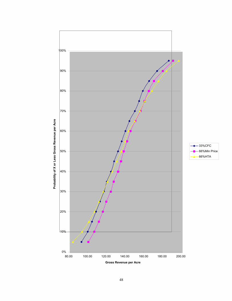
When CRC coverage is used, minimum price contracting 66 percent of the expected
production has the highest gross revenue at the 10 and 50 percent levels, with $108 and
$139 per acre, respectively. Using a HTA contract on 66 percent of the expected
production has the highest gross revenue at the 90 percent level with $185 per acre. Results
for these two strategies as well as three comparison strategies with CRC coverage are listed
in Table 16.
Table 16. Gross Revenue Per Acre of Marketing Strategies Combined with the 65 Percent Coverage Level of CRC Insurance
Base
33% CFC
33% Min Price 33% Puts
66% Min
Price
66% HTA
Mean 138 136 142 142 138
Std. Deviation 26 28 30 28 35
10% 106 100 106 108 85
25% 118 113 120 120 113
50% 136 133 138 139 137
75% 156 155 162 161 162
90% 173 175 182 181 185
46
Sensitivity Analysis
For all insurance products, the minimum price contracts were the most consistent
marketing strategies, being in the top three over all percentage levels. The factors affecting
the minimum price contracts, which allow them to consistently outperform the other
marketing strategies, can be ranked by a sensitivity analysis. A sensitivity analysis
identifies the input distributions that are significant in determining the value of the output
variable through multivariate stepwise regression. The output for this analysis, which was
conducted on the 33 percent level of minimum price contracting with 65 percent CRC
coverage, is shown in the tornado graph in Figure 3. The longer bars at the top of the graph
represent the most significant independent variables, while moving down the graph, the
Yield 1 = Wheat yield, Yield 2 = Corn Yield and Yield 3 = Soybean yield. Price 1 = Wheat price, Price 2 = Corn Price and Price 3 = Soybean price.
Regression Sensitivity for Gross Revenue Per Acre33% Min Price/D3
Coefficient Value
-.50 .00 .50 1.00
Basis 3 / Formula / C10
.027
Basis 1 / Formula / C8
.062
Price 2 / Formula / C3
-.168
Price 3 / Formula / C4
.351
Yield 3 / Formula / C7
.382
Yield 2 / Formula / C6
.427
Price1 / Formula / C2 .5
Yield1 / Formula / C5 .713
Std b coeffcalculated atend of bars
-1.00 -.50 .00 .50 1.00
47
Basis 1 = Wheat basis and Basis 3 = Soybean basis. Figure 3. Tornado Graph of Sensitivities of the 33 Percent Minimum Price Contracting Strategy Combined with 65 Percent CRC Coverage bars become shorter and the independent variables they represent become less significant.
Wheat yield is the most significant variable, specified by “yield 1,” followed by wheat
price, “price 1.” Corn price and yield are specified as “price 2” and “yield 2.” Soybean
price and yield are “price 3” and “yield 3.”
These independent variables have the same ranking of significance for all other
minimum price contracting strategies analyzed, but with differing values of the
standardized beta coefficient, shown at the end of the bars.
Stochastic Dominance Test
A second method of selecting efficient strategies would be to use a stochastic
dominance test. This test can be conducted by graphing the cumulative distribution
functions of each strategy, Figure 4. The probability of X or less gross revenue per acre is
on the Y-axis, and the gross revenue per acre is on the X-axis. A strategy will first-order
stochastically dominate another if the probability of realizing X or more dollars of gross
revenue per acre is at least as large as the probability of realizing X or more dollars of
gross revenue per acre for the second strategy for all values of X. The graph shows that the
66 percent minimum price contracting strategy first-order stochastically dominates the 33
percent cash forward contracting strategy. These two strategies, however, do not dominate
the 66 percent HTA contracting strategy, which demonstrates that stochastic dominance
can only be used as a partial decision criterion that can eliminate some inferior alternatives.
Mean-Variance Test A third decision criteria is the mean-variance (M-V) test. This test may be used for long-
run decision making. In the long run, the average gross revenue per acre would be
48
0%
10%
20%
30%
40%
50%
60%
70%
80%
90%
100%
80.00 100.00 120.00 140.00 160.00 180.00 200.00 Gross Revenue per Acre
Pro
babi
lity
of X
or L
ess
Gro
ss R
even
ue p
er A
cre
33%CFC 66%Min Price 66%HTA
49
studied in order to see if it is at a cash flow breakeven level. If it is, then a decision may be
made to raise a crop even if there is a chance of a loss that year because those losses may
be made up in following years in order to approach the current average.
This test can be conducted by plotting the mean and the variance, in this case, the
standard deviation, of particular strategies. The mean is on the X-axis, and the standard
deviation is on the Y-axis, Figure 5. The further up and to the left on the graph that the
strategy lies, the more appealing it is. If there is no obvious “best” strategy, as in Figure 5,
the decision will be based on the location of the farmer’s utility curve within the graph.
However, the set of efficient choices can be narrowed by eliminating M-V dominated
alternatives. In this case, the 33 percent cash forward contract is dominated by all other
strategies. The 33 percent puts are dominated by the 33 percent minimum price strategy.
The 33 percent minimum price/33 percent puts strategy is dominated by the 66 percent
minimum price strategy and leaves three M-V efficient choices: base, 33 percent minimum
price, and 66 percent minimum price. Depending on the level of risk aversion and the
producer’s ability to bear risk, the optimal strategy can be chosen from these three M-V
efficient strategies.
Single Crop Scenarios
The gross revenue per acre cumulative distributions of the single crop strategies
tested can be found in Tables B.1 through B.9 in Appendix B. Since the IP and RA
insurance coverages were not found to be as beneficial as CRC and MPC in the whole farm
analysis, they were not included in the single crop scenarios.
Figure 4. Stochastic Dominance Test of CRC Marketing Strategies.
50
Figure 5. Mean-Variance Test of CRC Marketing Strategies.
135.00
136.00
137.00
138.00
139.00
140.00
141.00
142.00
143.00
25.00 26.00 27.00 28.00 29.00 30.00 Standard Deviation Dollars Per Acre
Mea
n G
ross
Rev
enue
Per
Acr
e
Base 33%CFC 66%Min Price 33%Puts 33%Min Price 33%Puts 33% Min Price
51
Insurance Products Compared
In the single crop scenarios, each crop was tested individually with CAT, MPC, and
CRC insurance coverage. The marketing strategies included were the base strategy and the
three minimum price alternatives offered in the whole farm scenario. Seven other strategies
included the use of 33 and 66 percent put options, 33 percent futures hedging, 33 percent
cash forward contracts, 33 percent HTA contracts, and 33 percent cash forward contracts
combined with 33 percent put options.
The type of insurance selected for each crop was done in a similar manner as for the
whole farm. The insurance and marketing alternatives were again analyzed to find out if
their use increased the gross revenue per acre for that particular crop. The results of the
comparison indicate the same effects as in the whole farm scenario, except for one
difference. No insurance product produced an average gross revenue per acre larger than
the base strategy in soybeans. Because of the assumption that CAT coverage is carried by
most farmers, it was used in the insurance comparison for soybeans. For soybeans, CRC
and MPC coverage produced higher gross revenue at the 5 and 10 percent levels over CAT
coverage. Since this is a low coverage level and gross revenue is less for CRC than for
CAT at all other levels, CAT coverage was used for soybeans in the secondary whole farm
analysis. CRC performed much the same as it did in the whole farm scenario for wheat and
corn, becoming beneficial at the 15 to 20 percent levels.
Marketing Strategies Compared
As with the whole farm scenario, the three strategies with the highest gross revenue
per acre were selected at each percentage level in each scenario. These levels can be found
in the highlighted cells in the tables in Appendix B. Minimum price contracting 66 percent
52
of the expected production was the only marketing strategy that was in the top 3 strategies
for all percentage levels up to the 85 percent level in soybeans with CAT coverage. From
the 75 to 95 percent level, using a HTA contract on 33 percent of the expected production
had the highest gross revenue per acre.
Minimum price contracting 66 percent of the expected production as well as
minimum price contracting 33 percent of the expected production combined with
purchasing put options on 33 percent of the expected production were the 2 strategies
which were in the top 3 from the 10 to 90 percent levels in the wheat and corn scenarios
with CRC. Results are listed in Table 17.
Secondary Whole Farm Scenario
Combining the insurance products and marketing strategies specified for each
individual crop, four whole farm strategies were analyzed. The results can be found in
Table 18. The first strategy, strategy #1, uses the strategies that were specified for each
individual crop and includes minimum price contracting 66 percent of the expected
production of soybeans while using CAT coverage. Wheat and corn are covered by CRC
while minimum price contracting 33 percent of their expected production combined with
the purchase of put options on 33 percent of the expected production.
53
Table 17. Gross Revenue Per Acre for Single Crop Analysis of Marketing Strategies with Wheat and Corn Having CRC Insurance and Soybeans Having
CAT Insurance
66% Min Price 33% Min Price
33% Puts
33% HTA Wheat (CRC)
Mean 123 123 119
Std. Deviation 31 31 30
10% 84 85 83
25% 99 99 94
50% 118 119 115
75% 143 143 139
90% 161 163 159
Corn (CRC)
Mean 140 140 137
Std. Deviation 58 59 58
10% 78 76 78
25% 93 92 88
50% 127 126 121
75% 175 175 174
90% 220 222 219
Soybeans (CAT)
Mean 166 163 162
Std. Deviation 44 45 50
10% 107 104 97
25% 135 132 127
50% 166 164 163
75% 195 193 195
90% 223 223 225
54
Table 18. Gross Revenue Per Acre of the Four Strategies Tested in the Secondary Whole Farm Simulation
Strategy #1 Strategy #2 Strategy #3 Strategy #4 Wheat
And Corn
CRC with 33% Min Price and
33% Puts
CRC with 33% Min
Price and 33% Puts
CRC with 66%
Min Price
CRC with 66% Min
Price Soybeans CAT with 66%
Min Price CRC with 66% Min
Price
CAT with 66% Min Price
CRC with 66% Min
Price Mean 143 142 144 142
Std. Deviation 31 30 31 29
10% 105 106 106 108
20% 116 115 117 116
30% 124 123 125 124
40% 131 130 132 130
50% 139 138 140 138
60% 148 146 149 147
70% 157 155 158 156
80% 168 166 168 167
90% 185 182 184 182
The second strategy, strategy #2, is the same as the first except the specification for
CAT coverage on soybeans is changed to CRC coverage. In the third strategy, strategy #3,
wheat and corn retain the CRC coverage while soybeans are covered by CAT. The
marketing strategies are changed to include minimum price contracting 66 percent of the
expected production of all three crops. The fourth strategy, strategy #4, is similar to the
third, except the insurance coverage on soybeans is switched from CAT coverage to CRC.
55
Strategies Compared
The first and second strategies, which include the marketing strategy that combines
minimum price contracting and put options, are stochastically dominated by the third
strategy, which only includes minimum price contracting. The fourth strategy has a higher
gross revenue per acre than the third up to the 10 percent level because CRC insurance is
used on soybeans in that strategy and provides greater down side protection. At levels
higher than 10 percent, the values of the third strategy continue to increase over the fourth
because CAT coverage is used on soybeans, which incurs a lower cost than CRC does. A
person classified as a Risk Avoider may choose the fourth strategy, minimum price
contracting 66 percent of the expected production with CRC coverage, which is one of the
strategies specified as being optimal in the initial whole farm scenario while a Calculator
may find the third strategy more appealing.
Using a whole farm cash flow breakeven value of $155 per acre, the results indicate
that the breakeven level will not be reached until the 70 percent level for all strategies
tested. This result is slightly better than the strategies in the initial whole farm scenario
where a majority of the strategies tested did not break even until the 75 percent level.
Model Comparison
To compare the Bullock and the AgRisk models, several strategies using the same
input data were run with both models. A base strategy that included no marketing strategies
or insurance products was run as well as a strategy that included CRC with no marketing
strategies. The base strategy was also run with and without the consideration of the LDP in
the Bullock model. Five strategies, with and without the LDP, that included marketing
strategies were also run with CRC coverage.
56
The results of all the strategies, including the base, indicate that the AgRisk model
consistently underestimates the values at each level by $10 to $15 when compared to the
strategies from the Bullock model that consider the LDP. The most important factor in this
difference is that the AgRisk model does not consider the LDP. The Bullock model
calculates a LDP based on the county loan rate that is entered in the model. An average
LDP of $24 per acre for soybeans, $6 per acre for wheat, and $1 per acre for corn, which
were calculated by the Bullock model, will allow its output values to be larger than those
from AgRisk.
When all comparison strategies are run in the Bullock model without an LDP
payment, the AgRisk model begins to increase over the Bullock model at the 20 to 50
percent levels, Table 19. The differences are not very large, with the greatest difference of
$10 per acre coming at the 80 to 95 percent levels.
To explain the remaining differences in the output from the two models, the means
by which each estimates the price and yield random variables was explored. Viewing the
graphical representation of the yield distribution calculated by the AgRisk model shows
that it is not truncated at a minimum or maximum value. There are negative values shown
at the low end of the distribution and very large values at the high end. Also indicating that
the distribution is not truncated is the fact that, by using the indicator bars below the graph,
the model will calculate a percentage of the time the yield value will fall between the
lowest negative number and zero. AgRisk uses “non-parametric empirical distributions to
model prices and yields” (Miranda, 1999).
57
Table 19. Gross Revenue Per Acre Output Comparison of Bullock and AgRisk Models, Where the Bullock Model is Calculated with and without the Inclusion of an LDP on the Crops.
Base CRC Insurance Only Bullock
(LDP) Bullock
(No LDP) AgRisk Bullock (LDP)
Bullock (No LDP) AgRisk
Mean = 139 125 130 138 124 129 Std Dev = 31 28 30 26 25 26 5% Perc = 88 83 80 100 90 90 20% Perc = 113 101 103 114 102 105 35% Perc = 127 112 117 125 111 116 50% Perc = 139 122 129 136 120 127 65% Perc = 151 132 142 147 132 139 80% Perc = 163 148 157 159 144 153 95% Perc = 190 173 183 186 170 177
66% Puts 33% CFC 33% Puts Bullock
(LDP) Bullock
(No LDP) AgRisk Bullock (LDP)
Bullock (No LDP) AgRisk
Mean = 141 127 129 137 123 125 Std Dev = 31 23 26 33 22 26 5% Perc = 98 93 91 90 89 85 20% Perc = 112 107 105 107 102 101 35% Perc = 126 115 115 121 113 112 50% Perc = 138 125 126 131 122 123 65% Perc = 151 134 138 148 130 136 80% Perc = 164 143 152 164 141 150 95% Perc = 193 167 176 194 163 172
33% Min Price 66% Min Price Bullock
(LDP) Bullock
(No LDP) AgRisk Bullock (LDP)
Bullock (No LDP) AgRisk
Mean = 140 126 129 142 128 130 Std Dev = 28 24 27 29 23 26 5% Perc = 100 94 91 101 95 91 20% Perc = 115 105 104 115 108 105 35% Perc = 127 113 115 127 116 116 50% Perc = 138 123 126 139 125 127 65% Perc = 149 133 138 151 134 139 80% Perc = 161 145 153 164 145 154 95% Perc = 190 170 179 193 170 179
33% CFC 33% Min Price 33%Puts Bullock
(LDP) Bullock
(No LDP) AgRisk Bullock (LDP)
Bullock (No LDP) AgRisk
Mean = 135 121 125 141 127 130 Std Dev = 29 22 26 30 23 26 5% Perc = 93 90 87 99 94 91 20% Perc = 108 101 101 113 107 105 35% Perc = 121 111 112 127 116 116 50% Perc = 131 119 123 139 126 127 65% Perc = 145 127 135 151 135 139 80% Perc = 160 139 149 165 144 153 95% Perc = 186 163 173 195 168 178
58
Since the Bullock model uses a truncated normal yield distribution, the base model
was run with and without the truncation values specified to allow for a better comparison
of the models. The Bullock model does not allow a negative minimum yield value because
actual yields cannot fall below zero so that limit remained in place. Entering a large
number such as 9,999,999 eliminated the maximum limit. The simulation results from the
Bullock model indicate that eliminating the maximum yield changes the values per acre in
each strategy compared by no more than $0.16. For the comparison of the two models, the
maximum yield limit was eliminated.
The distribution used for price, the second source of variability in the model, was
also compared. The Bullock model uses a lognormal distribution where all values of X are
greater than zero and the distribution is skewed to the right. The graphical representation of
the “non-parametric price distributions” (Miranda, 1999) in the AgRisk model show a
distribution that appears normal with a minimum value of zero. The graphs are produced
through the use of “kernel smoothing techniques” (Miranda, 1999). Since a lognormal
distribution is skewed to the right, it helps to explain why the quasi-normal AgRisk output
values begin to constantly increase over the Bullock model.
A difference also occurs in the calculation of the average yield for a crop. The
AgRisk model will input average county yields that are retrieved from its database in years
that the individual farm does not have a yield. In the Bullock model, those years are not
calculated in the mean.
59
CHAPTER 6
SUMMARY AND IMPLICATIONS
Over the past decade, there have been government policy changes as well as
climactic occurrences that have led to increased price and yield risk faced by farmers. With
a 54 percent decline in median net farm income on farms enrolled in the North Dakota
Farm and Ranch Business Management Education Program from 1993-98, research is
needed to assist farmers in developing strategies to manage those risks. The main goal of
this study was to evaluate risk-management strategies that integrate responses to both
production and price risk that are faced by grain farmers in Cass County, North Dakota.
The first objective of this study was to analyze the effectiveness of integrated
marketing and crop insurance alternatives in reducing gross revenue per acre variability. A
second objective was to develop risk-management strategies for Cass County grain farms
based on that analysis. A final objective was to compare available risk-management
software, particularly the simulation model developed by Bullock and the AgRisk model
developed by Schnitkey, Miranda, and Irwin.
This study analyzed the effects that the use of crop insurance products and
marketing alternatives had on the gross revenue per acre for an individual farm in Cass
County. Individual farm yield data for wheat, corn, and soybeans were gathered from the
American Farm Bureau Insurance Agency in Fargo. Basis and forward contract prices were
gathered from Hunter Grain Company. Price and yield correlations were determined by
using county-level yields, and crop reporting district and state level prices. The Bullock
model was used to determine the gross revenue per acre cumulative distributions of each
strategy.
60
Crop insurance products and marketing strategies were analyzed individually to
determine if they were effective in minimizing down side risk and combined to determine
if integration created synergies. A whole farm scenario analysis was run that included
integrated strategies that implemented the same insurance coverage and marketing
alternatives for each crop. A strategy was selected based on the comparative advantages of
its gross revenue cumulative distribution. A single crop scenario was then run where the
integrated strategies were analyzed on each individual crop. The optimal strategies,
selected in the same manner as in the whole farm analysis, for each crop from the single
crop analysis were then combined in a secondary, whole farm scenario analysis.
Several general conclusions can be drawn for situations similar to the representative
farm. When analyzed at the individual crop level, the use of crop insurance at the 65
percent level minimizes down side risk in wheat and corn, but not significantly in
soybeans. Marketing alternatives generally increase the up side potential of gross revenue
per acre while doing little to minimize the down side risk. The integration of crop
insurance products and marketing alternatives creates a synergy at the lower levels of value
at risk, where the down side risk is located. However, the use of integrated strategies does
not increase the chances of achieving a cash flow breakeven gross revenue per acre over
the base strategy, which did not include insurance or marketing alternatives. The breakeven
level is not reached until the 70 percent level which means that, 7 out of 10 years, the farm
will not cash flow.
Integrated Risk Management Strategy Implications
Even though individual situations are different, it has been demonstrated that the
use of risk-management strategies that integrate the use of insurance products and
61
marketing alternatives minimizes the gross revenue per acre down side risk potential.
There were several strategies that outperformed others, and there were strategies that are
clearly inferior, even to the base strategy. In an individual farm decision process, the
inferior strategies will be eliminated from consideration, and a decision will be made on
the remaining strategies based on the risk attitude and financial situation of the farmer. On
this representative farm, it appears that minimum price contracting in conjunction with
crop revenue coverage produces the best results when analyzing the minimization of down
side risk and the increased up side potential. These results occurred in both the initial and
secondary whole farm scenarios. With similar results coming from both scenarios, it
appears that the only benefit from analyzing each crop separately and then combining them
into a whole farm scenario is the understanding of how each crop is affected by the
strategy.
The synergies that are present when insurance and marketing alternatives are
combined indicate that the use of crop insurance can eliminate fears associated with
forward contracting and futures hedging--mainly the fear of inadequate yields not being
able to offset a short futures position or meet the forward contract specifications. Crop
revenue coverage insurance is most effective in this aspect in all crops except soybeans.
One possible reason for the discrepancy in soybeans is the differential in the loan rate and
the contracting prices offered. Because the loan rate is higher than the predicted future
price, hedging with futures prices at the current level is not necessary.
The results will also be affected by the current level of prices received by farmers
for the specific crops relative to the level of production costs associated with each crop.
Currently, the prices received by farmers for their crops is quite low relative to the cost of
production, as demonstrated by the difficulty of achieving a breakeven cash flow. With
62
commodity prices at such a level, the marketing alternatives that establish a price floor,
such as minimum price contracts, while allowing for up side potential will be the most
beneficial. If the prices received are relatively high and the need to realize an increase in
price is not as great, cash forward contracts may be more beneficial than minimum price
contracts. Cash forward contracts also establish a price floor but do not incur the cost of
minimum price contracts.
These differences demonstrate that this method of analyzing risk management
strategies cannot be used as the only source of information when making a decision on
which strategy to use. It is only one tool to be used in the decision-making process.
Model Implications
Although there are differences in the output of the two models tested, they both are
beneficial in the decision making process. Once the main cause of the difference in the
output from the AgRisk model relative to the Bullock model was identified and accounted
for, the results became somewhat similar thus lending viability to the use of the AgRisk
model as a tool in a farmer’s risk-management decision making process.
Because AgRisk is a stand-alone program and the calculation process could not be
directly observed, the results were suspect. However, comparing the results with those
from the Bullock model, where the calculation process could be verified, and finding that
they were similar provided confidence that AgRisk could be used effectively. Because
there are still differences present and because it is rather easy to use, AgRisk would be
more appropriate to be used to arrive at a “ballpark” figure for a general analysis by a
producer.
63
Since the Bullock model is spreadsheet based, the process of calculating the output
variable can be verified. The model does calculate a LDP payment, which allows for a
more accurate representation of the gross revenue per acre. This process lends to the
credibility of the model and the results it produces.
Because of these advantages, the Bullock model seems to be better suited for a
more in depth study of the effects of risk management strategies on gross revenue per acre.
However, a difficulty in the use of the model may arise if an individual is not proficient in
the use of spreadsheet software and, in particular, the operation of the @RiskTM add-on
software. The use of the Bullock model may be more appropriate for individuals who do
analysis for producers and make recommendations about the types of risk-management
strategies that appear to be beneficial.
Limitations of Study and Suggestions for Further Research
A limitation faced by this study is that it used data from only one farm in Cass
County. Even though individual farm yield data was used instead of county data in order to
capture the possibility of higher yield variability, every farm will be different. Also, the
values used to calculate the cash flow breakeven level will vary among farms. Again, every
farm situation will have a different budget that needs to be analyzed separately.
This study may be used as a guide for producers and analysts in studying risk-
management strategies. To assist in the individual decision-making process, further study
will need to be done with yield data and budget amounts from the individual farm.
64
REFERENCES
American Farm Bureau Insurance Agency. Personal communication, Fargo, ND, 1999. Bierman, Harold, Jr., Charles P. Bonini, and Warren H. Hausman. Quantitative Analysis for Business Decisions. 7th ed. Richard D. Irwin, Homewood, IL, 1986. Bullock, David. “Simulation Model.” Unpublished Model, Risk Management Specialist, Minnesota Department of Agriculture, St. Paul, 1999. Carlson, Richard E., Dennis P. Todey, and Sterling E. Taylor. “Midwestern Corn Yield and
Weather in Relation to Extremes of the Southern Oscillation.” Journal Production of Agriculture 9:347-352, 1996.
Farm Credit Services Agency, Cass County. Personal communication, Fargo, ND, 1999. Data Transmission Network, Agricultural Services, Omaha, NE, April 26, 1999. Edwards, William. “Catastrophic Crop Insurance.” FM-1852, Iowa State University
Extension, Ames, IA, March 1999. Edwards, William. “Financial Considerations in Managing Risks and Profits. ”In R.
Wisner, D. Baldwin and N. Blue (Ed.), Managing Risk and Profits, Midwest Plan Service, Ames, IA, 1998.
Elhard, A. Eugene. “Selecting Crop production and Marketing Plans to Minimize risk for
Farmers in Southeast Central North Dakota.” Unpublished Master’s Thesis, North Dakota State University, Fargo, February 1988.
Flaskerud, George. Basis for Selected North Dakota Crops. North Dakota State University
Extension Service, Fargo, 1997. Flaskerud, George and Sherry Dusek. “RISK: Ideas on Managing.” Unpublished Paper,
North Dakota State University Extension Service, Fargo, March 1996. Flaskerud, George and Richard Shane. Wheat Marketing Strategies. North Central
Extension Producer Marketing Committee Report No. 1, North Dakota State University Extension Service, Fargo, 1993.
Hofstrand, Don and William Edwards. “Multiple Peril Crop Insurance.” FM-1826, Iowa
State University Extension, Ames, March 1999. Hu, Bin. “Farmer Decision Analysis Under the Federal Crop Insurance Reform Act of
1994.” Unpublished Master’s Thesis, North Dakota State University, Fargo, June 1996.
65
Hunter Grain Company. Personal communication. Hunter, ND, 1999. Johnson, D. Demcey, George K. Flaskerud, Richard D. Taylor, and Vidyashankara
Satyanarayana. “Economic Impacts of Fusarium Head Blight in Wheat.” Agricultural Economic Report No. 396, Department of Agricultural Economics, North Dakota State University, Fargo, June 1998.
Knight, Frank H. “Risk, Uncertainty and Profit.” Houghton Mifflin, Boston, 1921. Koo, Won W. “U.S. – Canada Border Disputes in Grains.” Unpublished Paper, Northern
Plains Policy and Trade Research Center, North Dakota State University, Fargo, 1998.
Miranda, Mario J. “AgRisk 1.0 Technical Reference.” Unpublished Paper, The Ohio State
University, Columbus, May 1999. North Dakota Agricultural Statistics, “Annual Bulletin,” Fargo, ND, 1980-1998. North Dakota Farm and Ranch Business Management Annual Reports, North Dakota
Farm and Ranch Business Management (Program). North Dakota State Board for Vocational and Technical Education, Bismarck, ND, 1993-1997.
O’Toole, Sherry A. “Risk Analysis for North Dakota: Farming Without a Government
Program.” Unplublished Master’s Thesis, North Dakota State University, Fargo, May 1998.
Patrick, George F. “Managing Risk in Agriculture.” North Central Region Extension
Publication, No. 406, Purdue University, West LaFayette, IN, May 1992. Patrick, George F. “Producers’ Attitudes, Perceptions and Management Responses to
Variability.” Risk Analysis for Agricultural Production Firms: Concepts, Information Requirements and Policy Issues, Proceedings of ‘An Economic Analysis of Risk Management Strategies for Agricultural Production Firms,’ New Orleans, March 1984. AE-4574, Department of Agricultural Economics, University of Illinois at Urbana-Champaign, July 1984.
Ray, Daryll E. and Kelly H. Tiller. “U.S. Agricultural Exports: Projected Changes Under
FAIR and Potential Unanticipated Changes.” Paper presented at the Western Agricultural Economics Association meeting, Reno, NV, 1997.
Swenson, Andrew. Personal communication. North Dakota State University Extension
Service, Fargo, June 1999.
66
Swenson, Andrew L. “Financial Characteristics of North Dakota Farms 1995-1997.” Agricultural Economics Report No. 403, Department of Agricultural Economics, North Dakota State University, Fargo, August 1998.
Swenson, Andrew L. and Cole R. Gustafson. “Financial Characteristics of North Dakota
Farms 1993-1995.” Agricultural Economics Report No. 358, Department of Agricultural Economics, North Dakota State University, Fargo, August 1996.
Swenson, Andrew and Ron Haugen. “Projected 1999 Crop Budgets South Valley North
Dakota.” Farm Management Planning Guide Section VI, Region 6B, North Dakota State University Extension Service, Fargo, December 1998.
USDA, Economic Research Service. “Uruguay Round Agreement on Agriculture: The
Record to Date.” Agricultural Outlook, Washington, DC, December 1998, pp 28-33.
USDA, National Agriculture Statistical Service, “Agricultural Statistics Annual Bulletin,”
Washington, DC, 1987 and 1997. Wisner, Robert N. “Risk, Cash-flow, and Profit Management Considerations for the 1998-
99 Grain Outlook.” Paper for presentation at the AAEA Annual Meeting, Salt Lake City, August 1998.
Wisner, Robert N., Dean Baldwin, and Neal Blue. “Foreword.” In R. Wisner, D. Baldwin
and N. Blue (Ed.), Managing Risks and Profits, Midwest Plan Service, Ames, IA, 1998.
Wisner Robert N., E. Dean Baldwin, and Neal E. Blue. “Integrated Production and Price
Risk Management: Impacts on Level and Variability of Corn and Soybean Producers’ Net Returns.” Unpublished Paper. Department of Economics, Iowa State University, Ames, and The Ohio State University, Columbus, 1998.
Wisner, Robert and Darrel Good. “Managing Risks and Profits.” In R. Wisner, D. Baldwin
and N. Blue (Ed.), Managing Risk and Profits, Midwest Plan Service, Ames, IA, 1998.
Tabl
e A.
1. G
ross
Rev
enue
Per
Acr
e fo
r CAT
Cov
erag
e w
ith S
elec
ted
Mar
ketin
g St
rate
gies
Nam
e
Base
33
%
CFC
66
%
CFC
33
% M
in
Pric
e 66
% M
in
Pric
e 33
% B
asis
Fi
xed
66%
Bas
is
Fixe
d 33
%
HTA
66
%
HTA
M
inim
um
= 65
.34
40.8
8 -1
4.41
65
.20
64.7
6 61
.11
56.4
9 43
.49
-5.2
9
Max
imu
m =
24
0.10
25
1.31
26
2.76
24
8.21
25
6.49
23
7.24
23
4.32
25
4.21
26
8.61
Mea
n =
139.
86
137.
07
134.
18
141.
85
143.
84
137.
07
134.
18
139.
90
139.
89
Std
Dev
=
29.2
9 32
.92
39.5
6 30
.41
31.9
3 29
.22
29.2
5 32
.99
39.6
4
Varia
nce
=
858.
08
1083
.75
1565
.36
925.
02
1019
.42
854.
03
855.
61
1088
.37
1571
.49
Mod
e =
12
3.29
16
1.34
13
6.25
16
2.12
15
4.94
14
3.35
13
3.73
14
4.86
14
8.51
Base
33
%
CFC
66
%
CFC
33
% M
in
Pric
e 66
% M
in
Pric
e 33
% B
asis
Fi
xed
66%
Bas
is
Fixe
d 33
%
HTA
6
6%
HTA
5%
93
.24
81.7
9 66
.81
93.8
8 94
.45
90.9
4 88
.00
84.4
9 72
.57
10%
10
2.12
95
.49
85.8
3 10
3.03
10
3.19
99
.58
96.7
7 97
.96
91.1
0 15
%
107.
34
102.
59
94.9
8 10
8.48
10
9.35
10
4.80
10
1.81
10
5.28
10
1.02
20
%
114.
48
109.
39
102.
79
114.
69
115.
81
111.
73
108.
36
111.
62
107.
42
25%
11
8.83
11
4.17
10
7.99
11
9.73
12
0.85
11
5.98
11
3.62
11
7.39
11
3.82
30
%
123.
01
119.
83
113.
10
124.
18
124.
99
119.
81
117.
28
122.
78
118.
59
35%
12
7.22
12
4.06
11
8.40
12
8.90
13
0.28
12
4.41
12
1.35
12
6.75
12
4.10
40
%
131.
54
127.
87
123.
23
133.
00
134.
46
128.
65
125.
89
130.
49
129.
42
45%
13
5.35
13
2.05
12
8.14
13
7.32
13
8.45
13
3.18
13
0.13
13
4.79
13
3.79
50
%
139.
75
136.
78
134.
31
141.
23
142.
83
137.
11
133.
86
139.
89
140.
49
55%
14
3.27
14
1.11
13
8.29
14
4.77
14
5.86
14
0.17
13
7.47
14
3.91
14
4.51
60
%
146.
19
144.
68
143.
05
148.
55
150.
51
143.
55
140.
77
147.
30
148.
64
65%
15
0.69
14
9.39
14
8.84
15
3.26
15
5.06
14
7.29
14
4.43
15
2.50
15
4.73
70
%
156.
44
154.
17
155.
06
158.
20
161.
43
153.
31
150.
08
157.
42
161.
16
75%
16
0.95
16
0.35
16
0.78
16
3.17
16
6.31
15
7.73
15
4.85
16
2.92
16
6.49
80
%
165.
72
164.
58
168.
08
167.
38
170.
33
162.
58
159.
57
167.
50
174.
03
85%
17
0.39
17
1.58
17
5.86
17
3.26
17
6.78
16
6.91
16
4.12
17
3.84
18
1.76
90
%
176.
60
180.
15
184.
49
180.
32
185.
02
173.
82
170.
99
182.
42
190.
54
95%
18
8.07
19
2.06
19
8.56
19
2.29
19
7.47
18
6.02
18
2.75
19
4.81
20
3.55
68
Tabl
e A.
1. (
Con
tinue
d)
Nam
e 33
% C
FC 3
3% P
uts
33%
CFC
33%
Fut
ures
33
% P
uts
66%
Put
s 33
% F
utur
es
66%
Fut
ures
33
% M
in P
rice
33%
Put
s M
inim
um =
37
.54
61.5
9 64
.54
62.5
3 62
.85
52.9
9 64
.33
Max
imum
=
263.
75
236.
71
252.
53
260.
71
270.
55
303.
92
260.
64
Mea
n =
13
8.78
13
6.82
14
1.57
14
2.76
13
9.62
13
9.44
14
3.56
St
d D
ev =
36
.34
29.0
6 31
.42
33.2
9 29
.86
32.5
4 33
.05
Varia
nce
=
1320
.83
844.
66
987.
08
1108
.45
891.
87
1058
.65
1092
.15
Mod
e =
12
8.22
14
3.78
13
1.79
14
8.34
15
2.34
13
9.95
10
2.11
33%
CFC
33%
Put
s 33
% C
FC 3
3% F
utur
es
33%
Put
s 66
% P
uts
33%
Fut
ures
66
% F
utur
es
33%
Min
Pric
e 33
% P
uts
5%
79.9
9 91
.23
92.1
1 90
.29
92.9
3 91
.77
92.0
8 10
%
93.4
3 99
.65
101.
25
100.
15
103.
22
100.
21
101.
87
15%
10
1.01
10
4.36
10
7.73
10
7.28
10
9.03
10
7.11
10
8.23
20
%
108.
04
111.
38
113.
38
112.
78
113.
44
112.
63
113.
88
25%
11
3.66
11
6.18
11
8.53
11
8.58
11
8.67
11
6.69
11
9.62
30
%
118.
99
120.
08
123.
24
123.
44
122.
32
121.
50
124.
34
35%
12
3.33
12
4.21
12
8.22
12
8.07
12
6.99
12
5.28
12
9.02
40
%
127.
85
128.
55
131.
97
133.
05
130.
90
129.
48
133.
52
45%
13
3.13
13
2.67
13
7.01
13
7.30
13
4.05
13
3.55
13
8.15
50
%
137.
65
136.
73
140.
77
141.
23
137.
65
137.
23
142.
02
55%
14
1.62
14
0.03
14
4.08
14
4.68
14
1.47
14
0.54
14
5.51
60
%
146.
04
143.
54
148.
43
150.
01
145.
84
144.
78
150.
45
65%
15
1.76
14
7.15
15
3.66
15
5.00
14
9.57
14
8.94
15
5.56
70
%
157.
40
152.
51
159.
13
160.
73
153.
25
152.
85
161.
11
75%
16
1.93
15
7.35
16
4.02
16
4.88
15
7.91
15
7.37
16
5.51
80
%
169.
52
161.
99
168.
11
170.
61
162.
89
164.
34
171.
26
85%
17
8.07
16
6.92
17
4.28
17
7.66
16
9.17
16
9.82
17
7.83
90
%
186.
03
173.
08
181.
47
187.
43
177.
18
178.
32
186.
97
95%
19
9.82
18
4.80
19
5.08
20
0.12
19
1.92
19
9.21
20
0.44
69
Tabl
e A.
2. G
ross
Rev
enue
Per
Acr
e fo
r CAT
Cov
erag
e w
ith S
elec
ted
Mar
ketin
g St
rate
gies
N
ame
Base
33
% C
FC
66%
CFC
33
% M
in P
rice
66%
Min
Pric
e 33
% B
asis
Fix
ed 6
6% B
asis
Fix
ed 3
3% H
TA
66%
HTA
M
inim
um =
80
.41
74.0
0 12
.38
80.6
8 80
.84
78.6
7 76
.18
76.6
2 21
.50
Max
imum
=
236.
14
247.
36
258.
80
244.
26
252.
53
233.
29
230.
37
250.
26
264.
66
Mea
n =
13
8.46
13
5.67
13
2.78
14
0.45
14
2.43
13
5.67
13
2.77
13
8.50
13
8.49
St
d D
ev =
26
.88
29.8
3 36
.21
27.9
3 29
.40
26.8
0 26
.82
29.9
0 36
.29
Varia
nce
=
722.
48
889.
67
1310
.83
780.
28
864.
56
718.
35
719.
05
894.
15
1316
.68
Mod
e =
14
0.05
12
1.67
13
1.66
15
8.14
13
9.99
11
4.63
13
6.74
13
8.27
13
6.81
Base
33
% C
FC
66%
CFC
33
% M
in P
rice
66%
Min
Pric
e 33
% B
asis
Fix
ed 6
6% B
asis
Fix
ed 3
3% H
TA
66%
HTA
5%
98
.93
89.6
1 76
.33
99.8
9 10
0.23
96
.19
93.8
7 92
.69
82.1
6 10
%
104.
53
97.4
1 87
.82
105.
08
105.
41
101.
50
98.6
2 10
0.36
93
.27
15%
10
9.44
10
2.99
95
.71
110.
04
110.
53
106.
53
103.
56
106.
05
101.
44
20%
11
3.58
10
8.10
10
1.61
11
4.69
11
4.99
11
0.86
10
7.78
11
0.77
10
6.61
25
%
117.
49
113.
23
106.
78
118.
91
119.
65
114.
82
112.
53
115.
91
112.
39
30%
12
1.54
11
7.76
11
1.60
12
3.04
12
3.90
11
8.88
11
5.87
12
0.53
11
7.18
35
%
125.
77
121.
36
115.
39
126.
72
127.
83
122.
67
119.
55
124.
34
121.
38
40%
12
9.65
12
5.81
12
1.23
13
1.25
13
2.62
12
6.89
12
3.95
12
8.52
12
7.05
45
%
133.
49
129.
57
126.
16
135.
20
136.
43
130.
24
127.
68
132.
44
131.
26
50%
13
7.16
13
4.15
13
1.15
13
8.59
14
0.15
13
4.36
13
1.61
13
7.10
13
6.98
55
%
140.
18
138.
02
135.
27
141.
86
143.
56
137.
54
134.
58
140.
59
141.
20
60%
14
3.64
14
1.28
14
0.11
14
5.30
14
7.32
14
0.54
13
7.53
14
4.17
14
5.63
65
%
147.
34
146.
33
145.
43
149.
59
152.
39
144.
52
141.
78
149.
38
151.
43
70%
15
2.81
15
1.27
15
1.11
15
5.01
15
8.13
15
0.10
14
7.25
15
4.42
15
7.21
75
%
157.
55
156.
83
156.
83
159.
89
162.
72
154.
55
151.
41
159.
09
162.
62
80%
16
2.09
16
0.64
16
4.53
16
4.35
16
6.95
15
9.14
15
5.92
16
3.87
17
0.22
85
%
166.
95
167.
78
171.
90
169.
86
173.
06
163.
34
160.
88
170.
15
177.
80
90%
17
3.23
17
6.20
18
0.54
17
7.33
18
1.35
17
0.45
16
7.23
17
8.46
18
6.59
95
%
184.
11
188.
11
194.
61
188.
33
193.
52
182.
06
178.
80
190.
85
199.
60
70
Tabl
e A.
2. (C
ontin
ued)
N
ame
33%
CFC
33%
Put
s 33
% C
FC 3
3% F
utur
es
33%
Put
s 66
% P
uts
33%
Fut
ures
66
% F
utur
es
33%
Min
Pric
e 33
% P
uts
Min
imum
=
70.6
6 77
.41
80.0
8 80
.11
66.0
0 55
.59
80.3
5 M
axim
um =
25
9.79
23
2.76
24
8.58
25
6.76
28
1.41
31
4.78
25
6.69
M
ean
=
137.
38
135.
42
140.
17
141.
35
138.
21
138.
04
142.
16
Std
Dev
=
33.2
7 26
.78
28.8
4 30
.66
28.6
9 32
.13
30.4
5 Va
rianc
e =
11
06.8
1 71
7.29
83
1.52
94
0.16
82
2.97
10
32.3
6 92
7.46
M
ode
=
137.
43
141.
39
122.
28
107.
70
127.
59
139.
82
134.
71
33
% C
FC 3
3% P
uts
33%
CFC
33%
Fut
ures
33
% P
uts
66%
Put
s 33
% F
utur
es
66%
Fut
ures
33
% M
in P
rice
33%
Put
s 5%
87
.43
95.9
6 97
.90
97.1
7 95
.50
91.8
3 98
.39
10%
95
.00
101.
16
104.
26
103.
73
103.
47
99.2
4 10
4.63
15
%
101.
73
106.
75
108.
64
107.
79
108.
22
105.
97
109.
21
20%
10
7.39
11
1.16
11
3.55
11
2.93
11
3.52
11
0.92
11
4.02
25
%
112.
63
114.
67
117.
61
117.
87
117.
53
115.
45
118.
85
30%
11
7.25
11
8.85
12
1.89
12
1.86
12
1.82
11
9.68
12
2.77
35
%
121.
83
122.
40
126.
37
125.
90
125.
93
123.
49
127.
19
40%
12
4.72
12
6.44
13
0.38
13
1.05
12
9.12
12
8.02
13
1.89
45
%
130.
50
130.
29
134.
65
134.
91
132.
98
131.
68
135.
74
50%
13
4.55
13
3.89
13
7.99
13
8.11
13
6.30
13
5.99
13
9.00
55
%
138.
49
137.
06
141.
37
141.
68
139.
82
139.
61
142.
73
60%
14
3.01
14
0.51
14
5.00
14
6.80
14
3.66
14
3.03
14
7.01
65
%
148.
55
143.
91
149.
98
152.
51
147.
18
147.
11
152.
35
70%
15
3.87
14
9.51
15
5.67
15
7.16
15
1.22
15
1.01
15
7.82
75
%
158.
24
154.
19
160.
34
161.
60
155.
11
156.
73
161.
90
80%
16
5.74
15
8.52
16
4.31
16
6.92
16
0.24
16
1.96
16
7.70
85
%
174.
11
163.
44
171.
04
173.
95
166.
04
167.
04
174.
21
90%
18
2.07
16
9.52
17
7.61
18
3.48
17
3.73
17
6.55
18
3.02
95
%
195.
86
180.
88
191.
13
196.
17
188.
74
195.
76
196.
50
71
Tabl
e A.
3. G
ross
Rev
enue
Per
Acr
e fo
r 65%
CR
C C
over
age
with
Sel
ecte
d M
arke
ting
Stra
tegi
es
Nam
e
Base
33
% C
FC
66%
CFC
33
% M
in P
rice
66%
Min
Pric
e 33
% B
asis
Fix
ed
66%
Bas
is F
ixed
33
% H
TA
66%
HTA
M
inim
um =
82
.88
82.2
6 42
.54
83.1
5 83
.30
81.8
3 80
.64
84.1
4 51
.66
Max
imum
=
238.
67
245.
47
256.
91
242.
37
250.
64
236.
39
233.
83
248.
37
262.
77
Mea
n =
13
8.43
13
5.63
13
2.74
14
0.41
14
2.40
13
5.63
13
2.74
13
8.46
13
8.46
St
d D
ev =
25
.81
28.4
9 34
.79
26.9
3 28
.47
25.7
3 25
.74
28.5
6 34
.86
Varia
nce
=
666.
22
811.
67
1210
.29
725.
39
810.
70
662.
26
662.
79
815.
84
1215
.52
Mod
e =
12
5.12
11
9.83
13
7.21
12
5.00
12
8.09
12
6.04
14
0.22
12
8.79
13
5.46
Base
33
% C
FC
66%
CFC
33
% M
in P
rice
66%
Min
Pric
e 33
% B
asis
Fix
ed
66%
Bas
is F
ixe
33%
HTA
66
% H
TA
5%
100.
15
93.7
1 78
.75
100.
33
101.
13
97.9
8 95
.48
96.4
3 84
.59
10%
10
5.88
10
0.33
88
.17
106.
82
107.
50
103.
49
100.
28
102.
79
94.2
4 15
%
111.
17
104.
94
96.3
6 11
2.10
11
2.33
10
8.44
10
5.10
10
7.33
10
1.72
20
%
115.
05
109.
37
101.
67
115.
86
116.
59
112.
45
109.
83
112.
22
107.
62
25%
11
8.16
11
3.43
10
7.04
11
9.68
12
0.13
11
6.03
11
3.29
11
6.52
11
2.61
30
%
122.
45
117.
71
111.
20
124.
17
124.
98
119.
77
116.
72
120.
17
117.
18
35%
12
6.42
12
0.69
11
5.68
12
7.44
12
8.26
12
3.49
12
0.47
12
3.85
12
1.35
40
%
129.
35
125.
49
120.
68
131.
50
132.
85
126.
95
124.
29
128.
58
126.
56
45%
13
3.52
12
8.74
12
6.03
13
5.17
13
6.18
13
0.92
12
7.97
13
2.06
13
1.82
50
%
136.
45
133.
07
130.
28
138.
03
139.
22
133.
93
130.
83
136.
38
136.
67
55%
13
9.28
13
6.87
13
4.83
14
1.45
14
2.77
13
6.60
13
3.88
13
9.22
14
0.50
60
%
142.
89
140.
79
139.
31
144.
47
146.
35
139.
87
136.
63
143.
64
144.
33
65%
14
5.98
14
5.31
14
4.36
14
9.14
15
1.72
14
3.37
14
0.41
14
8.77
15
0.84
70
%
151.
35
150.
83
149.
89
154.
08
157.
09
148.
72
145.
97
153.
19
156.
45
75%
15
6.01
15
5.42
15
5.57
15
8.44
16
1.33
15
3.36
15
0.24
15
8.00
16
1.59
80
%
160.
42
159.
58
162.
90
163.
02
166.
02
157.
31
154.
37
162.
71
169.
31
85%
16
5.29
16
6.16
17
0.46
16
9.22
17
1.41
16
2.43
15
9.50
16
8.33
17
6.20
90
%
173.
05
174.
59
179.
53
176.
51
180.
85
170.
22
166.
46
176.
98
184.
78
95%
18
3.01
18
7.26
19
3.06
18
7.27
19
1.63
18
0.66
17
7.56
18
9.19
19
7.92
72
Tabl
e A.
3. (C
ontin
ued)
N
ame
33
% C
FC 3
3% P
uts
33%
CFC
33%
Fut
ures
33
% P
uts
66%
Put
s 33
% F
utur
es 6
6% F
utur
es
33%
Min
Pric
e 33
% P
uts
Min
imum
=
78.9
2 81
.13
82.5
5 82
.58
79.2
6 76
.97
82.8
2 M
axim
um =
25
7.90
24
3.96
24
6.69
25
4.87
29
4.58
32
7.94
25
4.80
M
ean
=
137.
34
135.
38
140.
14
141.
32
138.
18
138.
01
142.
13
Std
Dev
=
32.0
9 25
.77
27.8
7 29
.75
28.1
3 31
.89
29.5
6 Va
rianc
e =
10
30.0
0 66
3.90
77
6.47
88
5.34
79
1.33
10
17.2
8 87
3.76
M
ode
=
116.
65
134.
64
114.
59
135.
97
125.
95
141.
14
132.
82
33%
CFC
33%
Put
s 33
% C
FC 3
3% F
utur
es
33%
Put
s 66
% P
uts
33%
Fut
ures
66%
Fut
ures
33
% M
in P
rice
33%
Put
s 5%
91
.40
97.9
1 99
.14
97.8
4 97
.96
94.5
6 99
.75
10%
98
.06
102.
87
105.
86
105.
30
104.
06
100.
12
106.
48
15%
10
2.97
10
8.48
11
0.47
11
0.29
10
8.71
10
6.16
11
0.90
20
%
108.
21
111.
95
114.
70
114.
39
113.
89
110.
34
115.
52
25%
11
2.88
11
5.81
11
8.40
11
8.61
11
7.34
11
4.48
11
9.71
30
%
116.
80
119.
49
122.
91
122.
27
121.
48
118.
76
123.
69
35%
12
1.29
12
3.52
12
6.76
12
7.52
12
5.22
12
2.91
12
8.09
40
%
125.
08
126.
68
131.
06
131.
06
128.
07
126.
49
132.
11
45%
13
0.12
13
0.18
13
3.86
13
4.49
13
2.11
13
0.83
13
5.31
50
%
133.
78
133.
76
137.
39
137.
46
135.
43
135.
00
138.
23
55%
13
7.81
13
6.89
14
0.38
14
1.26
13
9.40
13
8.46
14
2.02
60
%
142.
57
139.
63
144.
34
146.
01
143.
53
142.
06
146.
54
65%
14
7.77
14
3.06
14
9.39
15
1.58
14
6.59
14
5.91
15
2.00
70
%
152.
67
148.
51
154.
63
155.
91
150.
94
151.
19
156.
46
75%
15
7.35
15
2.96
15
9.05
16
0.68
15
4.83
15
6.37
16
1.56
80
%
164.
96
157.
07
163.
28
166.
36
159.
43
161.
54
166.
90
85%
17
2.52
16
1.76
16
9.88
17
2.81
16
5.68
16
6.91
17
3.28
90
%
180.
88
169.
97
177.
36
182.
14
173.
37
178.
21
181.
69
95%
19
4.25
18
0.17
19
0.06
19
4.28
18
9.42
19
9.07
19
4.61
73
Tabl
e A.
4. G
ross
Rev
enue
Per
Acr
e fo
r 65%
RA
Cov
erag
e w
ith S
elec
ted
Mar
ketin
g St
rate
gies
N
ame
Base
33
% C
FC
66%
CFC
33
% M
in P
rice
66%
Min
Pric
e 33
% B
asis
Fix
ed
66%
Bas
is F
ixed
33
% H
TA
66%
HTA
M
inim
um =
76
.26
49.2
6 1.
63
76.0
5 75
.44
73.2
2 68
.60
51.8
8 10
.75
Max
imum
=
233.
75
244.
96
256.
40
241.
86
250.
14
230.
89
227.
97
247.
86
262.
26
Mea
n =
13
5.26
13
2.47
12
9.58
13
7.25
13
9.24
13
2.47
12
9.58
13
5.30
13
5.29
St
d D
ev =
27
.66
31.4
3 38
.30
28.8
6 30
.47
27.5
9 27
.61
31.5
0 38
.37
Varia
nce
=
764.
90
987.
95
1466
.52
833.
02
928.
25
761.
06
762.
48
992.
26
1472
.03
Mod
e =
12
8.95
10
4.08
10
3.26
12
9.12
12
7.42
12
5.61
13
2.22
14
6.57
14
2.13
Base
33
% C
FC
66%
CFC
33
% M
in P
rice
66%
Min
Pric
e 33
% B
asis
Fix
ed
66%
Bas
is F
ixed
33
% H
TA
66%
HTA
5%
93
.43
81.5
1 66
.20
93.5
6 93
.31
90.3
7 87
.83
83.3
1 72
.40
10%
99
.57
92.7
7 82
.38
99.9
2 10
0.62
97
.10
94.0
7 95
.49
88.0
4 15
%
105.
79
100.
46
91.1
1 10
6.40
10
6.80
10
2.83
99
.57
102.
90
96.8
3 20
%
110.
09
104.
97
98.2
2 11
0.67
11
1.27
10
7.47
10
4.70
10
8.04
10
3.61
25
%
114.
00
109.
84
103.
51
114.
92
115.
94
110.
99
108.
49
112.
60
109.
42
30%
11
7.45
11
4.72
10
8.95
11
9.09
12
0.08
11
5.28
11
2.47
11
7.73
11
4.45
35
%
123.
10
118.
65
113.
33
124.
32
125.
58
119.
84
116.
91
121.
61
119.
40
40%
12
7.47
12
3.27
11
8.80
12
8.85
12
9.52
12
4.71
12
1.81
12
6.29
12
4.65
45
%
130.
78
127.
12
124.
21
132.
07
133.
84
127.
71
125.
15
130.
01
129.
41
50%
13
4.36
13
2.25
12
9.22
13
6.12
13
7.59
13
1.45
12
8.59
13
5.33
13
5.05
55
%
137.
56
135.
66
133.
17
139.
47
141.
46
134.
79
132.
02
138.
36
139.
13
60%
14
1.43
13
9.41
13
8.02
14
2.95
14
4.92
13
8.19
13
5.14
14
2.22
14
3.38
65
%
144.
85
144.
17
143.
66
147.
69
150.
16
142.
13
139.
43
146.
75
149.
93
70%
15
0.36
14
8.87
14
9.12
15
2.88
15
5.54
14
7.58
14
4.85
15
1.77
15
5.69
75
%
154.
99
154.
44
154.
95
157.
13
160.
24
151.
80
148.
85
157.
13
160.
64
80%
15
9.46
15
8.64
16
2.33
16
1.65
16
4.58
15
6.27
15
3.23
16
1.51
16
8.17
85
%
164.
08
165.
38
169.
86
167.
35
170.
55
160.
64
157.
94
167.
75
175.
67
90%
17
0.69
17
3.96
17
9.02
17
3.97
17
9.77
16
8.06
16
4.99
17
6.42
18
4.28
95
%
181.
72
185.
74
192.
55
186.
55
191.
12
179.
67
176.
65
188.
45
197.
41
74
Tabl
e A.
4. (C
ontin
ued)
N
ame
33%
CFC
33%
Put
s 33
% C
FC 3
3% F
utur
es
33%
Put
s 66
% P
uts
33%
Fut
ures
66
% F
utur
es
33%
Min
Pric
e 33
% P
uts
Min
imum
=
45.9
2 73
.69
72.9
2 70
.92
76.5
8 71
.06
72.7
1 M
axim
um =
25
7.40
23
0.36
24
6.18
25
4.36
26
4.27
29
7.64
25
4.29
M
ean
=
134.
18
132.
22
136.
97
138.
15
135.
01
134.
84
138.
96
Std
Dev
=
35.0
3 27
.42
29.9
3 31
.91
28.3
1 31
.16
31.6
6 Va
rianc
e =
12
27.2
3 75
1.69
89
6.09
10
18.2
5 80
1.51
97
1.09
10
02.3
3 M
ode
=
116.
05
127.
80
132.
91
133.
94
127.
42
140.
66
106.
17
33%
CFC
33%
Put
s 33
% C
FC 3
3% F
utur
es
33%
Put
s 66
% P
uts
33%
Fut
ures
66
% F
utur
es
33%
Min
Pric
e 33
% P
uts
5%
78.2
5 90
.42
91.3
8 90
.20
93.7
4 90
.52
91.5
1 10
%
89.9
3 97
.18
98.1
0 97
.74
100.
65
97.6
2 98
.82
15%
98
.58
102.
55
105.
36
104.
74
105.
08
103.
88
105.
97
20%
10
4.34
10
7.56
10
9.20
10
8.84
11
0.14
10
8.04
10
9.88
25
%
109.
51
111.
09
114.
02
113.
75
114.
21
111.
96
114.
77
30%
11
3.89
11
5.16
11
8.94
11
9.46
11
8.19
11
5.97
11
9.96
35
%
118.
28
119.
05
123.
84
123.
51
121.
75
120.
33
124.
49
40%
12
3.14
12
4.23
12
7.16
12
8.88
12
5.48
12
4.53
12
9.35
45
%
128.
54
127.
34
131.
95
132.
07
128.
94
128.
56
133.
06
50%
13
2.52
13
1.16
13
5.27
13
5.71
13
2.53
13
2.61
13
6.33
55
%
136.
58
134.
36
139.
00
139.
48
136.
12
135.
70
140.
34
60%
14
0.84
13
8.01
14
3.20
14
4.81
14
0.59
13
9.90
14
4.95
65
%
146.
71
141.
57
147.
60
150.
23
143.
97
142.
96
149.
95
70%
15
1.87
14
7.11
15
3.15
15
4.96
14
7.96
14
7.14
15
5.42
75
%
156.
22
151.
60
157.
81
159.
22
152.
16
152.
42
159.
51
80%
16
3.60
15
5.64
16
1.95
16
4.62
15
7.00
15
8.07
16
5.48
85
%
171.
88
160.
66
168.
23
171.
49
163.
20
163.
52
171.
61
90%
18
0.11
16
8.22
17
5.21
18
1.14
17
1.01
17
1.98
18
0.62
95
%
193.
74
178.
45
188.
81
193.
77
185.
57
192.
85
194.
09
75
Tabl
e A.
5. G
ross
Rev
enue
Per
Acr
e fo
r 65%
IP C
over
age
with
Sel
ecte
d M
arke
ting
Stra
tegi
es
Nam
e Ba
se
33%
CFC
66
% C
FC
33%
Min
Pric
e 66
% M
in P
rice
33%
Bas
is F
ixed
66
% B
asis
Fix
ed
33%
HTA
66
% H
TA
Min
imum
=
80.6
5 65
.90
13.1
7 80
.59
80.2
7 79
.53
74.9
1 68
.11
22.2
9 M
axim
um =
23
5.30
24
6.51
25
7.95
24
3.41
25
1.68
23
2.44
22
9.52
24
9.41
26
3.81
M
ean
=
137.
68
134.
89
132.
00
139.
67
141.
65
134.
89
131.
99
137.
72
137.
71
Std
Dev
=
26.7
8 30
.17
36.8
6 27
.95
29.5
4 26
.70
26.7
2 30
.24
36.9
3 Va
rianc
e =
71
6.93
91
0.43
13
58.6
4 78
1.31
87
2.51
71
3.00
71
4.12
91
4.69
13
64.0
5 M
ode
=
139.
04
126.
39
138.
31
120.
63
136.
32
133.
59
133.
85
122.
96
143.
68
Ba
se
33%
CFC
66
% C
FC
33%
Min
Pric
e 66
% M
in P
rice
33%
Bas
is F
ixed
66
% B
asis
Fix
ed
33%
HTA
66
% H
TA
5%
96.9
9 85
.74
75.0
4 97
.63
97.9
8 94
.30
91.3
1 88
.73
80.4
4 10
%
103.
28
97.7
8 85
.36
104.
17
104.
54
100.
57
98.0
6 99
.87
89.7
8 15
%
109.
13
102.
78
94.3
9 10
9.89
11
0.37
10
6.21
10
3.34
10
5.63
99
.91
20%
11
3.57
10
8.58
10
1.26
11
4.39
11
4.92
11
0.98
10
8.17
11
1.20
10
6.25
25
%
117.
45
113.
64
106.
64
118.
59
119.
00
114.
51
112.
08
115.
96
112.
28
30%
12
0.69
11
7.39
11
1.15
12
2.22
12
3.31
11
8.22
11
5.16
12
0.04
11
6.40
35
%
125.
15
120.
94
115.
50
126.
22
127.
46
122.
23
119.
52
123.
87
121.
24
40%
12
9.05
12
5.43
12
0.57
13
0.37
13
2.17
12
6.17
12
3.65
12
8.35
12
6.45
45
%
133.
19
128.
82
125.
55
134.
69
136.
04
129.
95
127.
48
131.
96
130.
90
50%
13
6.66
13
3.47
13
0.77
13
8.17
13
8.90
13
3.74
13
0.67
13
6.54
13
6.59
55
%
139.
14
137.
21
134.
71
141.
11
142.
97
136.
52
133.
98
139.
84
140.
67
60%
14
3.00
14
0.74
13
9.60
14
4.56
14
6.78
13
9.77
13
6.92
14
3.64
14
4.91
65
%
146.
60
145.
74
144.
90
149.
23
151.
55
143.
83
141.
06
149.
02
150.
69
70%
15
1.91
15
0.42
15
0.66
15
4.42
15
6.85
14
9.12
14
6.40
15
3.42
15
7.12
75
%
156.
37
155.
83
156.
55
158.
85
161.
87
153.
34
150.
21
158.
59
162.
49
80%
16
1.01
16
0.27
16
3.94
16
3.41
16
6.11
15
8.19
15
4.95
16
3.06
17
0.35
85
%
165.
75
166.
93
171.
32
168.
52
172.
22
162.
24
159.
71
169.
30
177.
16
90%
17
2.24
17
5.50
18
0.57
17
6.06
18
1.36
16
9.51
16
6.38
17
7.97
18
5.82
95
%
183.
35
187.
26
194.
10
187.
78
192.
67
181.
21
178.
20
190.
00
198.
96
76
Tabl
e A.
5. (C
ontin
ued)
N
ame
33%
CFC
33%
Put
s 33
% C
FC 3
3% F
utur
es
33%
Put
s 66
% P
uts
33%
Fut
ures
66%
Fut
ures
33
% M
in P
rice
33%
Put
s M
inim
um =
62
.56
79.9
4 77
.31
75.3
0 76
.19
71.0
8 77
.25
Max
imum
=
258.
94
231.
91
247.
73
255.
91
262.
07
291.
87
255.
84
Mea
n =
13
6.60
13
4.64
13
9.39
14
0.57
13
7.43
13
7.26
14
1.38
St
d D
ev =
33
.78
26.6
1 28
.98
30.9
3 28
.06
31.2
7 30
.70
Varia
nce
=
1141
.29
707.
95
839.
71
956.
52
787.
32
977.
96
942.
22
Mod
e =
12
2.85
13
5.65
11
5.63
13
0.54
12
7.00
14
7.10
13
3.86
3
3% C
FC 3
3% P
uts
33%
CFC
33%
Fut
ures
33
% P
uts
66%
Put
s 33
% F
utur
es 6
6% F
utur
es
33%
Min
Pric
e 33
% P
uts
5%
83.0
1 94
.11
95.2
7 93
.75
97.0
5 93
.38
95.1
9 10
%
95.1
2 10
0.67
10
3.25
10
2.62
10
3.28
99
.90
103.
43
15%
10
1.55
10
6.47
10
8.69
10
7.46
10
7.40
10
6.26
10
8.98
20
%
107.
19
111.
12
113.
40
113.
22
112.
40
109.
93
113.
88
25%
11
2.30
11
3.81
11
7.41
11
7.59
11
6.91
11
4.43
11
8.21
30
%
117.
15
118.
12
121.
53
121.
41
121.
09
118.
84
122.
39
35%
12
0.65
12
1.92
12
5.83
12
5.77
12
4.99
12
2.24
12
6.70
40
%
124.
50
125.
94
130.
28
130.
71
127.
96
126.
55
131.
35
45%
13
0.12
12
9.49
13
3.80
13
4.51
13
0.82
13
0.74
13
5.49
50
%
133.
83
133.
60
137.
25
137.
35
135.
50
134.
66
138.
15
55%
13
8.01
13
6.41
14
0.71
14
1.05
13
8.76
13
7.66
14
1.85
60
%
142.
29
139.
67
144.
94
145.
92
142.
81
142.
14
146.
46
65%
14
7.70
14
3.29
14
9.15
15
1.84
14
6.23
14
6.27
15
1.63
70
%
153.
24
148.
46
154.
72
156.
31
149.
98
149.
57
157.
10
75%
15
7.63
15
3.19
15
9.36
16
1.01
15
4.16
15
4.90
16
1.85
80
%
165.
38
157.
26
163.
50
166.
25
159.
40
161.
16
166.
89
85%
17
3.43
16
2.46
16
9.92
17
3.12
16
5.00
16
5.69
17
3.70
90
%
181.
66
168.
68
178.
13
182.
69
172.
44
174.
91
182.
17
95%
19
5.29
18
0.29
19
0.28
19
5.32
18
7.12
19
3.06
19
5.65
77
Tabl
e B.
1. G
ross
Rev
enue
Per
Acr
e fo
r Sin
gle
Cro
p An
alys
is, W
heat
with
CAT
Insu
ranc
e C
over
age
33%
3
3% C
FC
33%
Min
Pric
e
33%
66
%
66%
33
%
33%
33
%
Nam
e B
ase
CFC
33
% P
uts
33%
Put
s M
in P
rice
Min
Pric
e Pu
ts
Puts
Fu
ture
s H
TA
Min
imum
=
39.2
4 17
.07
14.7
2 36
.39
38.7
4 38
.13
34.5
4 36
.89
40.4
1 21
.20
Max
imum
=
225.
95
213.
89
227.
72
225.
21
225.
95
225.
95
226.
62
223.
60
240.
96
216.
06
Mea
n =
11
9.34
11
6.68
11
8.33
12
3.00
12
1.35
12
3.31
12
2.65
12
0.99
11
9.07
11
9.46
St
d D
ev =
33
.27
35.9
3 38
.18
35.6
8 34
.06
35.2
9 36
.29
34.4
5 33
.60
36.1
3 Va
rianc
e =
11
06.9
4 12
90.8
9 14
57.4
8 12
72.7
3 11
60.3
4 12
45.1
4 13
17.2
0 11
86.6
7 11
28.9
1 13
05.2
6 M
ode
=
105.
45
99.5
2 10
9.10
12
6.32
12
2.78
12
7.75
16
7.84
13
4.10
12
7.59
98
.30
5%
64.3
9 56
.80
54.6
0 62
.10
64.4
4 64
.13
59.7
5 62
.10
66.9
0 58
.93
10%
77
.52
67.2
8 65
.62
76.7
1 78
.23
78.2
8 75
.24
76.1
7 76
.62
70.1
8 15
%
84.3
4 79
.11
76.9
7 85
.39
85.4
5 86
.15
83.7
1 84
.80
84.8
0 80
.41
20%
90
.57
86.4
7 86
.75
92.9
1 91
.69
92.4
0 92
.07
91.8
1 89
.67
88.4
5 25
%
95.9
6 92
.27
92.7
3 97
.15
96.8
7 98
.34
96.5
5 95
.90
95.1
3 95
.34
30%
10
1.25
97
.09
97.1
6 10
3.40
10
2.94
10
3.26
10
2.55
10
2.68
10
0.18
98
.65
35%
10
5.54
10
1.40
10
1.71
10
7.88
10
7.49
10
8.54
10
7.27
10
7.32
10
5.67
10
4.61
40
%
109.
85
108.
80
107.
88
112.
76
111.
31
113.
05
112.
34
111.
20
108.
88
110.
84
45%
11
3.44
11
1.94
11
4.53
11
7.18
11
5.93
11
7.45
11
7.55
11
5.23
11
2.70
11
5.47
50
%
117.
69
117.
59
120.
43
121.
29
119.
64
121.
68
122.
58
119.
94
116.
28
119.
81
55%
12
2.31
12
2.49
12
3.57
12
6.37
12
4.89
12
6.94
12
6.15
12
5.08
12
0.16
12
4.16
60
%
126.
85
127.
12
128.
81
130.
91
129.
40
131.
53
131.
75
128.
96
125.
55
129.
58
65%
13
1.09
13
1.08
13
2.82
13
6.36
13
3.88
13
6.77
13
6.36
13
4.19
12
9.40
13
3.84
70
%
136.
44
135.
34
138.
87
142.
42
138.
63
141.
87
142.
49
139.
35
135.
89
138.
67
75%
14
2.30
14
0.79
14
3.59
14
7.33
14
5.43
14
8.15
14
6.59
14
4.88
14
0.89
14
3.65
80
%
148.
22
147.
32
148.
65
153.
36
151.
09
154.
64
152.
75
151.
21
146.
38
151.
03
85%
15
3.73
15
4.40
15
7.88
16
1.07
15
5.84
15
9.60
16
1.30
15
6.86
15
2.65
15
6.76
90
%
160.
45
160.
06
165.
68
167.
39
162.
77
166.
61
167.
94
162.
84
163.
13
163.
64
95%
17
2.88
17
7.25
18
3.21
18
3.71
17
9.93
18
2.17
18
5.05
17
9.18
17
6.53
17
9.76
79
Tabl
e B.
2. G
ross
Rev
enue
Per
Acr
e fo
r Sin
gle
Cro
p An
alys
is, W
heat
with
65%
MPC
Insu
ranc
e C
over
age
33%
3
3% C
FC
33%
Min
Pric
e
33%
66
%
66%
33
%
33%
33
%
Nam
e
Bas
e C
FC
33%
Put
s 33
% P
uts
Min
Pric
e M
in P
rice
Puts
Pu
ts
Futu
res
HTA
M
inim
um =
62
.53
52.5
4 50
.20
61.8
1 64
.01
64.1
6 59
.39
61.7
4 55
.42
56.6
7 M
axim
um =
22
2.70
21
0.65
22
4.48
22
1.96
22
2.70
22
2.70
22
3.37
22
0.35
23
7.72
21
2.82
M
ean
=
118.
68
116.
01
117.
66
122.
34
120.
68
122.
65
121.
98
120.
33
118.
41
118.
79
Std
Dev
=
30.0
5 31
.87
34.1
0 32
.24
30.7
6 31
.92
32.7
8 31
.04
31.5
1 32
.08
Varia
nce
=
903.
12
1015
.46
1162
.71
1039
.31
946.
27
1019
.15
1074
.69
963.
50
992.
99
1029
.41
Mod
e =
11
9.60
96
.28
105.
85
123.
10
119.
61
124.
52
119.
79
108.
35
124.
34
95.1
4 5%
75
.19
71.6
4 70
.10
75.5
5 76
.71
76.1
7 74
.06
75.5
5 72
.83
73.6
2 10
%
81.9
2 75
.65
73.5
5 81
.57
82.7
1 82
.96
80.1
7 81
.38
80.3
4 78
.14
15%
86
.03
79.0
6 77
.85
88.5
6 86
.85
88.2
9 87
.62
86.6
4 85
.94
82.4
6 20
%
90.6
9 85
.34
84.5
2 92
.38
91.7
4 93
.21
91.6
2 91
.46
90.9
0 86
.72
25%
95
.64
89.7
9 89
.58
97.1
2 96
.86
98.5
1 96
.06
96.5
7 96
.03
93.0
4 30
%
100.
34
93.8
4 93
.92
101.
65
101.
69
101.
91
100.
42
100.
63
101.
06
95.5
2 35
%
104.
00
98.1
5 98
.47
105.
71
105.
04
105.
96
104.
84
105.
11
104.
38
101.
37
40%
10
7.57
10
5.55
10
4.63
11
0.06
10
8.89
11
0.71
10
9.73
10
8.46
10
7.54
10
7.60
45
%
110.
87
108.
70
111.
28
115.
12
113.
14
114.
45
114.
76
112.
68
110.
47
112.
22
50%
11
5.22
11
4.34
11
7.18
11
8.28
11
6.97
11
8.88
11
9.47
11
7.11
11
4.43
11
6.56
55
%
119.
46
119.
25
120.
33
123.
13
121.
69
124.
47
122.
97
121.
86
119.
08
120.
92
60%
12
3.66
12
3.88
12
5.57
12
7.78
12
6.16
12
8.54
12
8.60
12
5.79
12
3.46
12
6.34
65
%
128.
29
127.
84
129.
58
133.
12
130.
94
133.
53
133.
42
131.
18
126.
98
130.
60
70%
13
3.29
13
2.10
13
5.63
13
9.19
13
6.15
13
8.82
13
9.24
13
6.20
13
3.46
13
5.43
75
%
139.
55
137.
55
140.
35
144.
08
142.
22
144.
90
143.
35
141.
64
138.
84
140.
40
80%
14
4.97
14
4.08
14
5.41
15
0.12
14
7.85
15
1.40
14
9.50
14
7.97
14
3.44
14
7.78
85
%
150.
48
151.
16
154.
63
157.
83
152.
60
156.
35
158.
06
153.
61
149.
68
153.
51
90%
15
7.21
15
6.82
16
2.44
16
4.15
15
9.53
16
3.36
16
4.69
15
9.60
15
9.89
16
0.40
95
%
169.
64
174.
00
179.
96
180.
47
176.
68
178.
93
181.
80
175.
94
174.
56
176.
52
80
Tabl
e B.
3. G
ross
Rev
enue
Per
Acr
e fo
r Sin
gle
Cro
p An
alys
is, W
heat
with
65%
CR
C In
sura
nce
Cov
erag
e
33
%
33%
CFC
3
3% M
in P
rice
33
%
66%
66
%
33%
33
%
33%
N
ame
B
ase
CFC
33
% P
uts
33%
Put
s M
in P
rice
Min
Pric
e Pu
ts
Puts
Fu
ture
s H
TA
Min
imum
=
63.2
4 65
.84
63.4
9 60
.97
63.3
2 63
.32
58.5
5 60
.90
64.3
4 61
.92
Max
imum
=
221.
20
209.
15
222.
98
220.
46
221.
20
221.
20
221.
87
218.
85
236.
22
211.
32
Mea
n =
11
8.94
11
6.28
11
7.93
12
2.60
12
0.95
12
2.91
12
2.24
12
0.59
11
8.67
11
9.06
St
d D
ev =
28
.74
30.0
1 32
.32
30.9
5 29
.47
30.6
5 31
.48
29.7
1 30
.84
30.2
4 Va
rianc
e =
82
5.91
90
0.52
10
44.4
1 95
7.89
86
8.21
93
9.41
99
0.77
88
2.94
95
1.22
91
4.53
M
ode
=
106.
03
105.
88
85.1
0 12
1.60
12
3.06
12
3.06
11
5.52
12
4.76
14
1.91
93
.60
5%
78.3
5 75
.36
73.6
4 78
.07
79.4
4 79
.39
76.0
0 78
.07
75.2
2 78
.13
10%
82
.18
80.0
2 78
.58
84.8
0 84
.09
84.2
8 83
.86
82.8
0 80
.37
82.9
1 15
%
87.8
0 84
.33
83.3
0 89
.67
88.7
6 89
.83
89.5
8 88
.77
85.0
6 87
.17
20%
92
.91
87.6
0 87
.05
93.8
3 94
.50
95.0
0 92
.90
93.5
4 90
.79
90.5
7 25
%
97.6
3 90
.87
91.1
5 98
.95
98.5
1 99
.23
97.9
5 98
.40
95.6
6 93
.68
30%
10
1.01
94
.73
94.0
5 10
2.76
10
2.60
10
3.79
10
2.06
10
2.28
10
0.85
97
.25
35%
10
4.85
97
.34
98.1
4 10
6.90
10
6.05
10
7.48
10
6.12
10
5.81
10
4.09
10
0.99
40
%
107.
81
104.
48
104.
40
110.
60
109.
87
110.
74
110.
66
108.
94
107.
29
106.
25
45%
11
1.04
10
7.48
11
0.19
11
5.61
11
2.92
11
4.89
11
5.39
11
3.01
11
1.21
11
1.15
50
%
115.
45
113.
10
115.
87
119.
32
117.
59
118.
22
119.
25
116.
93
114.
02
115.
40
55%
11
9.10
11
7.99
11
9.01
12
2.99
12
2.97
12
3.77
12
2.52
12
1.60
11
9.31
11
9.72
60
%
123.
69
122.
40
124.
11
127.
27
125.
41
127.
70
127.
30
124.
87
123.
05
125.
10
65%
12
7.44
12
6.59
12
8.46
13
2.28
13
0.73
13
3.13
13
2.38
13
0.01
12
7.00
12
9.63
70
%
131.
86
131.
14
134.
22
137.
79
134.
94
138.
43
137.
79
134.
97
133.
47
134.
30
75%
13
8.24
13
6.39
13
9.30
14
2.82
14
1.16
14
3.68
14
2.32
14
0.66
13
8.11
13
8.98
80
%
143.
68
142.
98
144.
93
148.
81
146.
54
150.
15
148.
56
147.
34
143.
20
146.
28
85%
14
9.51
14
9.66
15
3.54
15
6.35
15
1.16
15
5.10
15
7.17
15
2.20
15
0.52
15
2.01
90
%
155.
72
155.
32
161.
18
162.
65
158.
52
161.
86
163.
19
158.
10
158.
67
158.
90
95%
16
8.14
17
2.50
17
8.46
17
8.97
17
5.18
17
7.43
18
0.30
17
4.44
17
3.19
17
5.02
81
Tabl
e B.
4. G
ross
Rev
enue
Per
Acr
e fo
r Sin
gle
Cro
p An
alys
is, C
orn
with
CAT
Insu
ranc
e C
over
age
33%
3
3% C
FC
33%
Min
Pric
e
33%
66
%
66%
33
%
33%
33
%
Nam
e
Bas
e C
FC
33%
Put
s 33
% P
uts
Min
Pric
e M
in P
rice
Puts
Pu
ts
Futu
res
HTA
M
inim
um =
35
.62
9.07
3.
93
29.4
8 34
.62
33.6
0 30
.48
30.4
8 8.
62
11.2
7 M
axim
um =
39
4.23
37
7.50
38
5.43
38
9.09
39
4.23
39
4.23
38
9.09
38
9.09
41
0.15
38
3.48
M
ean
=
139.
75
134.
77
136.
34
143.
06
141.
49
143.
09
141.
32
141.
32
139.
33
139.
60
Std
Dev
=
66.9
9 68
.97
71.9
2 69
.79
67.6
3 68
.62
68.7
4 68
.74
68.5
0 69
.03
Varia
nce
=
4487
.59
4756
.92
5172
.48
4870
.76
4574
.17
4708
.85
4725
.02
4725
.02
4692
.68
4765
.25
Mod
e =
52
.41
163.
57
121.
98
128.
74
52.1
9 18
7.22
16
9.19
16
9.19
12
5.50
57
.86
5%
47.2
8 37
.34
33.3
1 44
.15
47.9
4 47
.29
44.3
1 44
.31
46.0
2 41
.90
10%
54
.73
48.9
6 44
.31
54.2
5 55
.23
55.2
6 53
.50
53.5
0 57
.41
53.4
0 15
%
65.6
4 56
.44
54.0
3 63
.89
65.8
8 65
.98
63.3
6 63
.36
70.8
3 61
.73
20%
76
.04
67.1
5 65
.49
74.7
4 76
.15
76.6
6 73
.61
73.6
1 79
.15
72.4
7 25
%
86.3
6 83
.22
80.3
1 85
.88
89.0
2 90
.15
85.8
8 85
.88
85.4
4 87
.11
30%
99
.13
93.8
2 92
.01
100.
80
100.
28
101.
78
99.5
6 99
.56
94.9
4 96
.55
35%
10
7.02
10
1.56
10
2.45
10
9.27
10
8.26
10
9.09
10
6.82
10
6.82
10
3.95
10
7.18
40
%
114.
54
109.
88
111.
85
119.
00
115.
01
117.
58
116.
62
116.
62
112.
67
116.
36
45%
12
2.72
11
7.97
12
2.18
12
8.56
12
5.55
12
6.07
12
6.31
12
6.31
12
0.90
12
3.76
50
%
133.
70
129.
52
131.
21
136.
67
135.
41
136.
51
134.
94
134.
94
128.
64
133.
13
55%
14
1.54
13
8.89
14
1.49
14
7.47
14
2.45
14
4.85
14
4.77
14
4.77
13
8.95
14
3.88
60
%
152.
09
147.
03
151.
46
157.
43
154.
30
156.
75
154.
82
154.
82
147.
67
152.
07
65%
16
0.71
15
7.38
16
2.70
16
6.12
16
2.86
16
4.23
16
3.88
16
3.88
15
9.17
16
2.17
70
%
172.
43
167.
51
171.
40
176.
65
174.
37
177.
07
174.
36
174.
36
169.
98
171.
99
75%
18
5.46
18
0.69
18
2.85
18
7.86
18
7.13
18
7.35
18
6.47
18
6.47
18
0.79
18
6.58
80
%
196.
14
194.
18
196.
66
202.
46
199.
86
201.
03
199.
06
199.
06
197.
98
199.
08
85%
20
9.52
20
8.42
21
3.27
21
8.87
21
2.63
21
4.33
21
2.75
21
2.75
21
0.88
21
1.73
90
%
230.
90
227.
42
229.
98
234.
72
230.
98
233.
36
229.
85
229.
85
229.
27
232.
18
95%
25
9.38
25
3.40
25
4.48
26
8.00
26
2.90
26
3.80
26
3.06
26
3.06
26
2.93
26
0.18
82
Tabl
e B.
5. G
ross
Rev
enue
Per
Acr
e fo
r Sin
gle
Cro
p An
alys
is, C
orn
with
65%
MPC
Insu
ranc
e C
over
age
33%
3
3% C
FC
33%
Min
Pric
e
33%
66
%
66%
33
%
33%
33
%
Nam
e
Bas
e C
FC
33%
Put
s 33
% P
uts
Min
Pric
e M
in P
rice
Puts
Pu
ts
Futu
res
HTA
M
inim
um =
61
.62
44.5
0 39
.36
61.6
3 63
.48
63.6
8 61
.63
61.6
3 29
.12
48.5
6 M
axim
um =
38
6.23
36
9.50
37
7.43
38
1.09
38
6.23
38
6.23
38
1.09
38
1.09
40
2.15
37
5.48
M
ean
=
137.
97
132.
99
134.
57
141.
29
139.
71
141.
32
139.
55
139.
55
137.
56
137.
82
Std
Dev
=
60.0
4 61
.46
64.3
1 62
.55
60.6
0 61
.50
61.5
3 61
.53
62.8
7 61
.53
Varia
nce
=
3604
.84
3776
.76
4135
.60
3912
.06
3672
.20
3782
.24
3785
.54
3785
.54
3952
.74
3786
.21
Mod
e =
73
.42
67.6
5 62
.52
67.3
9 81
.58
179.
22
73.7
1 73
.71
110.
20
71.7
8 5%
69
.03
65.2
7 60
.80
68.0
5 70
.81
70.5
2 68
.29
68.2
9 58
.27
69.2
7 10
%
73.4
8 67
.72
63.5
4 72
.20
74.3
4 74
.16
72.5
4 72
.54
68.6
7 71
.88
15%
78
.06
69.3
0 65
.87
75.3
9 78
.50
78.2
3 75
.39
75.3
9 75
.22
74.5
4 20
%
81.7
1 71
.56
69.9
3 80
.22
82.7
8 83
.36
79.1
7 79
.17
84.9
3 77
.28
25%
86
.57
76.2
3 76
.43
89.1
6 87
.03
88.7
9 87
.32
87.3
2 90
.31
82.0
4 30
%
94.5
3 86
.20
86.5
1 94
.66
94.9
3 96
.45
93.8
7 93
.87
95.7
5 89
.98
35%
99
.85
93.9
5 94
.82
101.
87
101.
24
101.
35
101.
05
101.
05
101.
33
99.3
6 40
%
106.
63
103.
48
105.
18
111.
22
107.
55
110.
32
109.
32
109.
32
110.
03
108.
49
45%
11
5.71
10
9.97
11
4.18
12
0.56
11
8.07
11
8.54
11
8.31
11
8.31
11
5.79
11
5.76
50
%
125.
70
121.
52
123.
21
129.
31
127.
41
128.
51
127.
20
127.
20
123.
26
125.
13
55%
13
3.69
13
0.89
13
3.49
13
9.47
13
4.82
13
6.95
13
6.77
13
6.77
13
2.87
13
5.88
60
%
144.
09
139.
03
143.
46
149.
43
146.
30
148.
75
146.
82
146.
82
141.
96
144.
07
65%
15
2.71
14
9.38
15
4.70
15
9.06
15
4.86
15
6.23
15
5.88
15
5.88
15
2.88
15
4.17
70
%
164.
65
159.
51
163.
40
168.
65
166.
48
169.
25
166.
61
166.
61
162.
73
163.
99
75%
17
7.46
17
2.69
17
4.85
17
9.86
17
9.13
17
9.35
17
8.47
17
8.47
17
2.79
17
8.58
80
%
188.
14
186.
18
188.
66
194.
46
191.
86
193.
03
191.
06
191.
06
190.
68
191.
08
85%
20
1.52
20
0.42
20
5.27
21
0.87
20
4.63
20
6.33
20
4.75
20
4.75
20
2.88
20
3.73
90
%
222.
90
219.
42
221.
98
226.
72
222.
98
225.
36
221.
85
221.
85
221.
27
224.
18
95%
25
1.38
24
5.40
24
6.48
26
0.00
25
4.90
25
5.80
25
5.06
25
5.06
25
5.12
25
2.18
83
Tabl
e B.
6. G
ross
Rev
enue
Per
Acr
e fo
r Sin
gle
Cro
p An
alys
is, C
orn
with
65%
CR
C In
sura
nce
Cov
erag
e
33
%
33%
CFC
3
3% M
in P
rice
33
%
66%
66
%
33%
33
%
33%
N
ame
B
ase
CFC
33
% P
uts
33%
Put
s M
in P
rice
Min
Pric
e Pu
ts
Puts
Fu
ture
s H
TA
Min
imum
=
64.2
0 61
.44
56.3
0 59
.06
64.2
0 64
.16
59.0
6 59
.06
53.9
3 63
.89
Max
imum
=
381.
22
364.
49
372.
42
376.
08
381.
22
381.
22
376.
08
376.
08
397.
14
370.
47
Mea
n =
13
7.10
13
2.12
13
3.69
14
0.41
13
8.83
14
0.44
13
8.67
13
8.67
13
6.68
13
6.94
St
d D
ev =
56
.69
57.6
4 60
.60
59.2
5 57
.26
58.1
8 58
.18
58.1
8 60
.45
57.7
2 Va
rianc
e =
32
13.2
0 33
22.5
9 36
72.6
4 35
10.2
5 32
79.1
8 33
85.1
7 33
85.1
1 33
85.1
1 36
54.7
3 33
31.4
8 M
ode
=
77.4
5 15
0.56
74
.29
115.
70
77.4
5 73
.15
109.
67
109.
67
73.4
8 78
.51
5%
73.8
0 70
.47
65.3
6 71
.81
73.9
4 73
.32
71.8
1 71
.81
63.8
7 74
.63
10%
78
.02
72.5
4 68
.50
75.7
7 78
.45
77.8
1 75
.77
75.7
7 69
.36
78.3
9 15
%
81.0
5 75
.75
72.0
5 81
.07
82.4
0 83
.15
80.7
0 80
.70
74.7
5 80
.41
20%
86
.63
79.3
6 76
.08
86.6
5 88
.77
88.8
8 86
.46
86.4
6 82
.04
83.7
7 25
%
91.4
4 83
.64
81.9
1 91
.64
92.3
9 93
.11
90.5
8 90
.58
88.1
6 88
.39
30%
96
.15
88.7
5 87
.65
96.8
6 97
.93
98.1
9 96
.71
96.7
1 95
.29
93.7
3 35
%
101.
53
94.5
4 93
.91
104.
31
102.
65
104.
87
103.
61
103.
61
102.
45
98.6
0 40
%
107.
38
100.
71
104.
28
113.
30
110.
24
111.
28
109.
74
109.
74
108.
03
105.
81
45%
11
5.63
10
7.41
11
3.35
11
8.99
11
7.64
11
9.72
11
7.33
11
7.33
11
6.10
11
3.25
50
%
122.
90
116.
70
119.
79
126.
22
124.
88
126.
88
123.
56
123.
56
122.
74
121.
07
55%
12
9.96
12
6.11
12
9.29
13
6.39
13
1.58
13
5.85
13
3.05
13
3.05
13
2.05
13
1.06
60
%
139.
96
135.
46
138.
67
145.
00
141.
55
144.
02
142.
92
142.
92
141.
42
139.
43
65%
14
7.70
14
4.37
14
9.78
15
4.10
14
9.85
15
1.84
15
1.09
15
1.09
15
1.87
14
9.16
70
%
159.
64
154.
50
158.
40
164.
77
161.
47
164.
24
161.
60
161.
60
160.
61
158.
98
75%
17
2.74
16
7.68
17
2.24
17
4.85
17
4.16
17
4.75
17
3.46
17
3.46
16
9.43
17
3.57
80
%
183.
13
181.
17
183.
65
189.
45
186.
85
188.
02
186.
05
186.
05
187.
83
186.
07
85%
19
6.51
19
5.41
20
0.26
20
5.86
19
9.62
20
1.32
19
9.74
19
9.74
20
0.53
19
8.72
90
%
217.
89
214.
41
216.
97
221.
71
217.
97
220.
35
216.
84
216.
84
216.
26
219.
17
95%
24
6.37
24
0.39
24
1.47
25
4.99
24
9.89
25
0.79
25
0.05
25
0.05
25
0.11
24
7.17
84
Tabl
e B.
7. G
ross
Rev
enue
Per
Acr
e fo
r Sin
gle
Cro
p An
alys
is, S
oybe
ans
with
CAT
Insu
ranc
e C
over
age
33%
3
3% C
FC
33%
Min
Pric
e
33%
66
%
66%
33
%
33%
33
%
Nam
e
Bas
e C
FC
33%
Put
s 33
% P
uts
Min
Pric
e M
in P
rice
Puts
Pu
ts
Futu
res
HTA
M
inim
um =
59
.79
43.3
8 39
.32
55.7
4 45
.71
59.1
2 58
.12
58.6
8 56
.05
25.1
0 M
axim
um =
31
2.33
28
6.88
31
4.38
30
8.27
30
8.67
31
2.33
30
6.23
30
8.26
34
9.43
31
5.02
M
ean
=
161.
93
159.
39
161.
19
163.
29
164.
07
166.
22
164.
62
163.
72
161.
72
161.
91
Std
Dev
=
41.4
2 43
.86
47.6
1 45
.27
45.6
3 43
.89
45.1
8 43
.63
43.5
5 49
.59
Varia
nce
= 1
715.
34
1923
.95
2266
.36
2049
.51
2081
.85
1926
.02
2041
.29
1903
.27
1896
.90
2459
.04
Mod
e =
18
0.30
15
5.73
19
5.16
10
1.02
17
7.52
20
5.37
19
4.86
14
5.79
15
0.24
16
2.62
5%
91
.42
85.9
0 82
.16
86.9
0 88
.34
91.2
9 87
.39
89.1
5 91
.21
74.1
5 10
%
106.
40
101.
92
100.
80
104.
18
105.
58
107.
35
104.
61
105.
67
105.
98
96.9
4 15
%
120.
87
113.
76
110.
44
117.
10
116.
23
121.
23
118.
35
118.
49
118.
04
111.
16
20%
12
7.36
12
0.61
12
0.23
12
4.31
12
4.63
12
9.23
12
5.72
12
7.03
12
6.15
11
9.08
25
%
132.
85
130.
31
128.
58
132.
03
133.
64
135.
06
132.
77
132.
09
132.
01
127.
15
30%
13
9.49
13
7.77
13
7.13
13
9.46
14
0.99
14
2.13
14
0.22
14
0.75
13
8.11
13
6.24
35
%
144.
82
143.
64
142.
29
144.
67
146.
96
148.
62
146.
50
145.
81
143.
60
143.
64
40%
14
9.83
14
9.02
15
0.40
15
1.88
15
2.80
15
4.32
15
2.96
15
3.63
14
9.31
15
0.53
45
%
155.
78
155.
18
157.
19
157.
80
160.
08
160.
06
159.
93
158.
66
154.
11
156.
88
50%
16
1.26
16
0.75
16
2.10
16
3.81
16
5.57
16
5.52
16
5.83
16
3.72
15
8.86
16
2.70
55
%
168.
01
164.
65
167.
62
168.
84
169.
69
171.
73
169.
94
169.
42
164.
88
168.
77
60%
17
3.48
17
0.97
17
1.85
17
2.76
17
4.57
17
6.02
17
4.23
17
3.22
16
9.67
17
3.98
65
%
178.
20
175.
22
176.
10
179.
11
178.
73
181.
60
180.
91
179.
61
174.
41
179.
86
70%
18
3.93
18
1.79
18
3.62
18
6.13
18
6.16
18
9.56
18
7.63
18
6.64
18
1.78
18
4.50
75
%
189.
73
189.
32
191.
41
192.
59
193.
47
194.
52
194.
26
192.
43
188.
11
194.
50
80%
19
5.65
19
5.87
19
8.74
19
9.13
20
0.81
20
1.22
20
0.77
19
7.97
19
5.13
20
2.34
85
%
203.
06
201.
03
208.
29
207.
83
209.
44
208.
77
209.
13
205.
92
204.
72
210.
88
90%
21
3.04
21
3.31
21
9.87
22
2.84
22
0.73
22
2.66
22
4.19
21
9.55
21
6.70
22
4.78
95
%
232.
02
229.
57
239.
42
237.
79
238.
37
237.
02
239.
19
235.
01
231.
91
242.
39
85
Tabl
e B.
8. G
ross
Rev
enue
Per
Acr
e fo
r Sin
gle
Cro
p An
alys
is, S
oybe
ans
with
65%
MPC
Insu
ranc
e C
over
age
33%
3
3% C
FC
33%
Min
Pric
e
33%
66
%
66%
33
%
33%
33
%
Nam
e
Bas
e C
FC
33%
Put
s 33
% P
uts
Min
Pric
e M
in P
rice
Puts
Pu
ts
Futu
res
HTA
M
inim
um =
95
.61
86.4
7 82
.40
88.7
8 88
.79
95.8
2 89
.94
91.9
7 74
.95
65.5
1 M
axim
um =
30
8.42
28
2.97
31
0.48
30
4.36
30
4.76
30
8.42
30
2.32
30
4.35
34
5.52
31
1.11
M
ean
=
159.
78
157.
24
159.
04
161.
14
161.
92
164.
07
162.
47
161.
57
159.
57
159.
76
Std
Dev
=
38.6
5 40
.78
44.5
9 42
.45
42.5
8 41
.10
42.3
4 40
.79
41.5
2 46
.45
Varia
nce
= 1
493.
66
1663
.40
1987
.99
1802
.11
1813
.16
1688
.90
1792
.89
1663
.78
1723
.87
2157
.97
Mod
e =
17
6.40
15
1.82
19
1.25
96
.53
95.4
2 20
1.46
19
0.96
19
1.88
16
5.68
87
.41
5%
99.4
0 94
.32
90.2
5 96
.65
96.1
5 10
1.07
97
.61
99.3
6 97
.37
87.5
0 10
%
107.
74
101.
57
99.8
2 10
5.05
10
4.60
11
0.40
10
7.32
10
6.34
10
9.17
98
.60
15%
11
8.86
11
0.08
10
7.25
11
5.07
11
2.43
11
9.96
11
5.98
11
6.42
11
8.22
10
7.68
20
%
124.
79
116.
70
116.
32
121.
92
120.
72
127.
03
122.
57
124.
47
124.
00
115.
95
25%
12
9.60
12
6.40
12
4.67
12
8.12
12
9.73
13
2.03
12
9.59
12
8.59
12
9.73
12
3.24
30
%
135.
91
133.
87
133.
22
135.
85
137.
08
138.
80
136.
72
136.
93
134.
88
132.
33
35%
14
0.94
13
9.73
13
8.38
14
0.80
14
3.05
14
4.75
14
2.67
14
2.38
14
1.05
13
9.73
40
%
145.
96
145.
11
146.
49
148.
05
148.
89
151.
02
149.
57
149.
75
146.
05
146.
63
45%
15
2.08
15
1.27
15
3.28
15
3.89
15
6.17
15
6.28
15
6.02
15
4.75
15
1.42
15
2.97
50
%
157.
64
156.
84
158.
19
159.
90
161.
66
161.
61
161.
92
159.
81
156.
10
158.
79
55%
16
4.10
16
0.75
16
3.71
16
4.93
16
5.78
16
7.82
16
6.03
16
5.51
16
1.36
16
4.86
60
%
169.
57
167.
06
167.
94
168.
85
170.
66
172.
11
170.
32
169.
32
165.
78
170.
08
65%
17
4.29
17
1.31
17
2.19
17
5.20
17
4.83
17
7.70
17
7.00
17
5.70
17
0.50
17
5.95
70
%
180.
02
177.
88
179.
71
182.
23
182.
26
185.
65
183.
72
182.
73
177.
87
180.
59
75%
18
5.82
18
5.41
18
7.50
18
8.68
18
9.56
19
0.61
19
0.36
18
8.52
18
4.20
19
0.59
80
%
191.
74
191.
96
194.
83
195.
22
196.
91
197.
31
196.
86
194.
06
191.
30
198.
43
85%
19
9.15
19
7.13
20
4.38
20
3.92
20
5.53
20
4.87
20
5.22
20
2.01
20
1.30
20
6.97
90
%
209.
14
209.
40
215.
96
218.
93
216.
82
218.
75
220.
29
215.
64
212.
79
220.
87
95%
22
8.12
22
5.66
23
5.51
23
3.88
23
4.46
23
3.11
23
5.28
23
1.10
22
8.01
23
8.48
86
Tabl
e B.
9. G
ross
Rev
enue
Per
Acr
e fo
r Sin
gle
Cro
p An
alys
is, S
oybe
ans
with
65%
CR
C In
sura
nce
Cov
erag
e
33
%
33%
CFC
3
3% M
in P
rice
33
%
66%
66
%
33%
33
%
33%
N
ame
B
ase
CFC
33
% P
uts
33%
Put
s M
in P
rice
Min
Pric
e Pu
ts
Puts
Fu
ture
s H
TA
Min
imum
=
94.4
7 88
.35
84.2
9 87
.18
89.8
0 94
.35
88.3
8 90
.41
94.8
2 82
.25
Max
imum
=
306.
74
281.
29
308.
80
302.
68
303.
08
306.
74
300.
64
302.
67
343.
84
309.
43
Mea
n =
15
9.34
15
6.81
15
8.61
16
0.71
16
1.48
16
3.64
16
2.04
16
1.14
15
9.13
15
9.33
St
d D
ev =
37
.37
39.6
6 43
.72
41.5
5 41
.59
40.0
8 41
.43
39.7
6 40
.23
45.5
4 Va
rianc
e =
139
6.65
15
72.7
3 19
11.0
7 17
26.0
5 17
29.8
1 16
06.7
5 17
16.5
0 15
80.5
2 16
18.8
5 20
73.5
3 M
ode
=
174.
72
157.
87
189.
66
164.
76
163.
45
126.
87
175.
41
140.
20
164.
00
181.
18
5%
102.
08
97.1
7 93
.10
96.4
3 10
0.09
10
2.05
97
.56
99.2
8 10
0.60
88
.46
10%
11
2.45
10
5.06
10
1.92
10
9.05
10
8.19
11
3.39
11
1.34
11
2.19
10
9.94
96
.92
15%
11
9.82
11
2.25
10
8.33
11
6.45
11
4.20
12
1.12
11
7.45
11
8.87
11
7.08
10
6.68
20
%
125.
47
118.
92
117.
34
122.
79
121.
77
126.
99
124.
10
124.
71
123.
60
117.
08
25%
13
0.97
12
5.50
12
5.50
12
8.32
12
9.03
13
3.29
12
9.33
13
1.13
12
8.33
12
4.54
30
%
135.
95
133.
70
132.
27
135.
28
136.
69
139.
43
136.
94
137.
38
133.
31
132.
44
35%
14
0.73
13
8.58
13
8.39
14
1.77
14
2.19
14
3.67
14
2.63
14
1.92
13
9.69
13
9.92
40
%
145.
48
143.
72
146.
11
147.
21
148.
60
150.
29
149.
29
148.
25
144.
75
146.
07
45%
15
0.77
15
0.18
15
1.94
15
2.97
15
5.35
15
5.04
15
5.04
15
3.44
15
0.21
15
2.24
50
%
156.
63
155.
92
157.
57
158.
41
160.
19
160.
75
160.
40
158.
87
155.
16
158.
36
55%
16
3.18
15
9.76
16
2.20
16
3.68
16
4.32
16
6.88
16
4.70
16
4.28
16
0.08
16
3.57
60
%
167.
96
165.
85
166.
45
167.
26
169.
47
170.
92
169.
00
168.
18
164.
62
169.
44
65%
17
2.61
17
0.18
17
0.81
17
4.45
17
4.44
17
7.25
17
5.56
17
4.77
16
9.98
17
4.27
70
%
178.
34
176.
94
178.
84
181.
51
180.
97
184.
27
182.
66
181.
75
176.
26
180.
49
75%
18
4.14
18
3.80
18
7.27
18
7.36
18
9.13
18
9.50
18
9.27
18
6.97
18
2.52
18
9.99
80
%
190.
06
190.
28
193.
68
193.
83
195.
74
195.
66
195.
37
192.
38
189.
62
197.
89
85%
19
7.47
19
5.45
20
3.65
20
2.30
20
4.06
20
3.19
20
3.54
20
0.33
19
9.62
20
5.81
90
%
207.
46
207.
72
214.
28
217.
25
215.
14
217.
07
218.
61
213.
96
212.
92
219.
19
95%
22
6.44
22
3.98
23
3.83
23
2.20
23
2.78
23
1.43
23
3.60
22
9.42
22
6.33
23
6.80
87