uci Background Basic MCMC Jumping Rules Practical Challenges and Advice Overview of Recommended Strategy Markov Chain Monte Carlo David A. van Dyk Statistics Section, Imperial College London Smithsonian Astrophysical Observatory, March 2014 David A. van Dyk MCMC
Transcript
uci
BackgroundBasic MCMC Jumping Rules
Practical Challenges and AdviceOverview of Recommended Strategy
Markov Chain Monte Carlo
David A. van Dyk
Statistics Section, Imperial College London
Smithsonian Astrophysical Observatory, March 2014
David A. van Dyk MCMC
uci
BackgroundBasic MCMC Jumping Rules
Practical Challenges and AdviceOverview of Recommended Strategy
Outline
1 BackgroundBayesian StatisticsMonte Carlo IntegrationMarkov Chains
3 Practical Challenges and AdviceDiagnosing ConvergenceChoosing a Jumping RuleTransformations and Multiple Modes
4 Overview of Recommended Strategy
David A. van Dyk MCMC
uci
BackgroundBasic MCMC Jumping Rules
Practical Challenges and AdviceOverview of Recommended Strategy
Bayesian StatisticsMonte Carlo IntegrationMarkov Chains
Bayesian Statistical Analyses: Likelihood
Likelihood Functions: The distribution of the data given themodel parameters. E.g., Y dist∼ Poisson(λS):
likelihood(λS) = e−λSλYS/Y !
Maximum Likelihood Estimation: Suppose Y = 3
0 2 4 6 8 10 12
0.00
0.10
0.20
lambda
likel
ihoo
d The likelihoodand its normalapproximation.
Can estimate λS and its error bars.David A. van Dyk MCMC
uci
BackgroundBasic MCMC Jumping Rules
Practical Challenges and AdviceOverview of Recommended Strategy
Bayesian StatisticsMonte Carlo IntegrationMarkov Chains
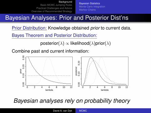
Bayesian Analyses: Prior and Posterior Dist’ns
Prior Distribution: Knowledge obtained prior to current data.
Bayes Theorem and Posterior Distribution:
posterior(λ) ∝ likelihood(λ)prior(λ)
Combine past and current information:
0 2 4 6 8 10 120.00
0.10
0.20
0.30
lambda
prio
r
0 2 4 6 8 10 120.00
0.10
0.20
lambda
post
erio
r
Bayesian analyses rely on probability theoryDavid A. van Dyk MCMC
uci
BackgroundBasic MCMC Jumping Rules
Practical Challenges and AdviceOverview of Recommended Strategy
Bayesian StatisticsMonte Carlo IntegrationMarkov Chains
Why be Bayesian?
Avoid Gaussian assumptionsMethods like χ2 fitting implicitly assume a Gaussian model.Many other methods rely on asymptotic Gaussianproperties (e.g., stemming from central limit theorem).
Bayesian methods rely directly on probability calculus.Designed to combine multiple sources of informationand/or external sources of information.Modern computational methods allow us to work withspecially-tailored models and methods.
Selection effects, contaminated data, observational biases,complex physics-based models, data distortion, calibrationuncertainty, measurement errors, etc.
David A. van Dyk MCMC
uci
BackgroundBasic MCMC Jumping Rules
Practical Challenges and AdviceOverview of Recommended Strategy
Bayesian StatisticsMonte Carlo IntegrationMarkov Chains
Simulating from the Posterior Distribution
We can simulate or sample from a distribution to learnabout its contours.With the sample alone, we can learn about the posterior.
Here, Y dist∼ Poisson(λS + λB) and YBdist∼ Poisson(cλB).
prior
lamS
0 2 4 6 8
0.0
0.2
0.4
0.6
0 2 4 6 8 10
0.0
0.2
0.4
posterior
lamS
joint posterior with flat prior
lamS
lam
B
0 2 4 6 81.
52.
02.
5
.
..
.
.
.
.
.
.
...
.
......
.
.
.
.
.
.
..
.
.
.
..
. .
.
..
.
..
.. .
.
.
..
.
..
.
.
.
.
.
.
.
.
.
..
.
..
.
.
.
. ... .
.
.
.
.
..
..
.
..
. .
..
.
.
.
.
.
.
..
.
.
.
.
...
.
.
..
.
.
.
. .
.
.
.
.
.
.
..
..
.
...
.
.
.
.
.
.
.
.
.
.
..
.
.
.. .... .
.
.
.
. . .
.
.
.
.
.
.
.
.
.
.
.....
..
.
.
.
. .
.
.
....
.
.
. .
.
..
..
..
..
.
.
.
.
.
. ...
.
.
.
.
.
..
.
...
.
..
. .
.
..
.
.
.
...
.
. .
.
.
.
..
..
..
.. . .
.
.
.
.
.
.
.
.
.
.
.
..
.
.
.
.
.
.
.
.
..
.
..
.
.
..
.
.
.
..
. .
.
.
.
..
.
.
.
.
..
.
..
.
..
.
.
.
..
.
. ..
.
.
..
.
.
.
.
.
.
.
.
. .
.
..
.
.
..
. .
.
.
.
.
.
.
..
.
.
.
.
.
.. .
.
.
...
..
.
.
. .
.
.
.
.
.
.
...
.. ..
.
. ..
..
.
..
.
.
.
.
.
.
.
..
.
...
.
.
.
.
..
. ..
.
.
.
. .
.. .
.
.
..
. ..
.
.
.
.
.
.
.
.
.
..
.
.
.
.
.
.
.
.
..
..
.
.
....
..
.
.
.
.
.
.
. ...
.
.
.
.
.
.
.
.
..
.. .
.
.
.
..
.
.
.
.
.
.
..
..
.
.
.
.
.
.
...
.
.
..
.
.
..
.
. ..
..
.
.
.
.
...
.
.
.
..
.
..
.
.
. .
.
.
.
.
.
.
.
.
.
.
..
..
.
..
..
. ..
. ..
.
.
. .
..
.
..
.
..
..
.
..
.
.
.
. .
.
.
.
..
.
.
.
.
.
.
.
.
.
.
.
.
.
.
.
.
..
..
.
.
.
.
.
.
. ..
.
.
.
.
.
.
.
.
..
.
.
.
.
.
..
.
.
..
..
...
.
.
.
.
.
.
.
.
..
.
.
..
...
.
.
..
.
.
.
..
.
..
.
.
.
.
..
.
.
.
.
.
.
.
.
..
..
...
.
.
.
.
..
.
.
.
...
.
..
.
.. .
.
..
..
.
.
.
.
.
.
..
.
...
.
.
.
...
.
.
.
.
.
.
.
.
.
..
.
.
..
.
.. .
.
..
..
.
.
.
.
...
..
.
.... ....
.
..
..
.
.
.
.
.
..
.
. .
.
. .
.
.
...
.
.
.
.
.
..
.
.
.
.
.
. .
.
.
.
.
.
. .
.
.
..
.
..
.. ..
.
..
..
.
.
.
..
..
. .
...
.
.
..
.. .
.
.
.
.
.
.
.
...
.
..
.
.
.
.
.
.
.
..
.
..
.
.
.
.
.
.
..
.
.
.
..
..
..
.
. ..
..
.
.
..
..
.
.
.
.
.
.
.
.
.
.
.
.
..
.
.
.
.
.. .
.
.
.
.. .
.
. .
..
.
..
.
..
.
.
.
.
.
.
.
.
..
.
.
.
.. ...
.
.
.
.
.
.
..
.
..
.
.
..
.
.. .. .
.
.
.
.
..
.
..
..
.
.
..
.
.
...
.
.
. ..
.
.
.
.
.
..
.
... .
.
.
..
. ..
.
.
..
.
.
.
.
.
.
.
.
..
.. .
..
.
. .
.
.
.
.
..
.
.
.
. .
.
. .
.
..
..
.
.
.
.
.
.
..
.
.
.
.
.
.
.
...
.
....
..
.
..
..
.
.
.
.
.
.
.
..
.
.
.
.
.
.
..
.
.
.
. .
..
.
.
..
.
. ..
..
.
. .
.
.
.
..
.
.
.
.
.
.
.
. .
.
.
.
.
...
.
.
.
..
.
..
..
.
.
.
.
. ..
.
.
...
.
..
.
.
.
..
...
.
.
.
.
.
.
.
. .
.
.
.
. .
.
..
.
.
.
.
.
.
.
.
.
.
.
.
.
.
.
...
.
.
...
..
.
.
.
.. .
.
.
.
.
. .
..
.
.. .
.
.
.
.
.
.
..
..
.
.
..
..
.
.
.
.
.
..
.
.
..
..
...
..
..
...
.
.
..
.
.
.
.
.
..
..
..
..
.
.
.
.
.
.
..
.
.
...
.
.
.
.
.
..
.
.
..
.
.
..
..
.
.
.
..
.
.
.
...
.
..
.
..
. ..
.
..
..
.
.
...
.
.
.
.
.
.
.
.
.
.
.
.
..
.
...
...
.
...
. .
.
. .
.
...
...
..
..
.
.
.
.
.
..
..
.
..
.
.
.
.
..
.
.
.
..
.
.
.
.
.
..
.
.
. ..
.
.
.
.
.
..
..
.
.
.
.
.
.
...
..
.
.
.
..
.
... .
.
.
.
..
.
.
.
.
.
.
.
. . .
.
....
.
.
..
.
..
...
.
.
.
...
.
.
.
.
.
.
.
..
..
.. .
.
.
.
.
.
.
..
..
....
.
.
.
..
...
.
.
.
.
..
. ..
.
.
.
...
.
..
.
..
.
..
.
.
.
.
. ..
..
.
.
.
.
..
.
.
.
.
.
..
.
.
.
.
.
.
.
... .
.
.
.
.
.
..
.
.
..
..
.
.. ..
..
.
..
.
.... .
. .
.
.
.
.
.
.
.
.
.
.
.
..
.
.
.
.
.
.
.
.
.
.
.. .
.
..
.
.
.
.
.
.
.
.
.
.
.
.
.
..
.
..
.
..
.
.
.
.
..
..
.
..
.
.
..
.
...
.
..
.
.
.
..
.
. .
.
.
.
..
.
.
. .
..
.
..
.
.
.
.
..
.
..... .
...
.
.
..
.
.
..
.
.
.
. ..
.
.. .
..
.
.
.
.
.. .
..
. ..
..
.
....
.
..
.
.
.
.
.
.
..
.
...
.
.
.
.
.
.
..
.
.
.
..
.
.
.
.. .
.
.
.
.
. ..
.
.
.
...
.
.
.
.
.
.
.
.
.
.
. ..
. .
.
.
.
..
.
. .
.
.
.
.
.
..
.
.
.
..
.
..
.
.
..
. .
..
.
.
.
.
.
.
.
.
.
..
.
.
.
..
.
.
.
.
.
.
.
.
.
..
.
.
.
.
.
..
.
.
.
.
.
. .
..
...
.
.
.
.
.
..
.
. ...
.
.
.
.
..
.
.
..
..
..
..
.
.
.
.
.
.
.
.
.
.
..
.
.
..
.
.
.
.
.
.
.
.
.
.
.
..
.
.
..
.
. ..
.
.
..
...
.
.
.
.
.
...
.
..
.
.
..
David A. van Dyk MCMC
uci
BackgroundBasic MCMC Jumping Rules
Practical Challenges and AdviceOverview of Recommended Strategy
Bayesian StatisticsMonte Carlo IntegrationMarkov Chains
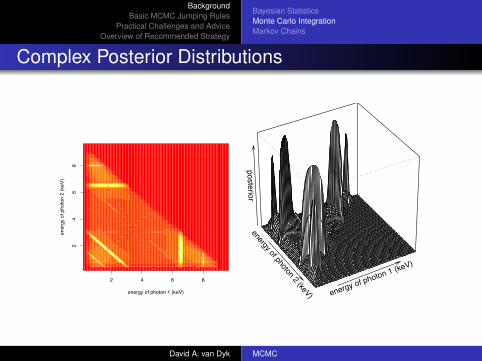
Model Fitting: Complex Posterior Distributions
Highly non-linear relationship among stellar parameters.
David A. van Dyk MCMC
uci
BackgroundBasic MCMC Jumping Rules
Practical Challenges and AdviceOverview of Recommended Strategy
Bayesian StatisticsMonte Carlo IntegrationMarkov Chains
Model Fitting: Complex Posterior Distributions
Highly non-linear relationships among stellar parameters.David A. van Dyk MCMC
uci
BackgroundBasic MCMC Jumping Rules
Practical Challenges and AdviceOverview of Recommended Strategy
Bayesian StatisticsMonte Carlo IntegrationMarkov Chains
Model Fitting: Complex Posterior DistributionsMultiple Modes
The classification ofcertain stars as fieldor cluster stars can
cause multiplemodes in the
distributions of otherparameters.
David A. van Dyk MCMC
uci
BackgroundBasic MCMC Jumping Rules
Practical Challenges and AdviceOverview of Recommended Strategy
Bayesian StatisticsMonte Carlo IntegrationMarkov Chains
Complex Posterior Distributions
David A. van Dyk MCMC
uci
BackgroundBasic MCMC Jumping Rules
Practical Challenges and AdviceOverview of Recommended Strategy
Bayesian StatisticsMonte Carlo IntegrationMarkov Chains
Complex Posterior Distributions
0 2 4 6 8 10
0.0
0.1
0.2
0.3
0.4
0.5
energy (keV)
post
erio
r den
sity
David A. van Dyk MCMC
uci
BackgroundBasic MCMC Jumping Rules
Practical Challenges and AdviceOverview of Recommended Strategy
Bayesian StatisticsMonte Carlo IntegrationMarkov Chains
Complex Posterior Distributions
2 4 6 8
24
68
energy of photon 1 (keV)
ener
gy o
f pho
ton
2 (k
eV)
energy of photon 2 (keV) energy of photon 1 (keV)
posterior
David A. van Dyk MCMC
uci
BackgroundBasic MCMC Jumping Rules
Practical Challenges and AdviceOverview of Recommended Strategy
Bayesian StatisticsMonte Carlo IntegrationMarkov Chains
Using Simulation to Evaluate Integrals
Suppose we want to compute
I =
∫g(θ)f (θ)dθ,
where f (θ) is a probability density function.If we have a sample
θ(1), . . . , θ(n)dist∼ f (θ),
we can estimate I with
In =1n
n∑i=1
g(θ(t)).
In this way we can compute means, variances, and theprobabilities of intervals.
David A. van Dyk MCMC
uci
BackgroundBasic MCMC Jumping Rules
Practical Challenges and AdviceOverview of Recommended Strategy
Bayesian StatisticsMonte Carlo IntegrationMarkov Chains
We Need to Obtain a Sample
Our primary goal:
Develop methods to obtain a sample from adistribution
The sample may be independent or dependent.Markov chains can be used to obtain a dependent sample.In a Bayesian context, we typically aim to sample theposterior distribution.
We first discuss an independent method:Rejection Sampling
David A. van Dyk MCMC
uci
BackgroundBasic MCMC Jumping Rules
Practical Challenges and AdviceOverview of Recommended Strategy
Bayesian StatisticsMonte Carlo IntegrationMarkov Chains
Rejection Sampling
Suppose we cannot sample f (θ) directly, but can find g(θ) with
f (θ) ≤ Mg(θ)
for some M.
1 Sample θ dist∼ g(θ).
2 Sample u dist∼ Unif (0,1).3 If
u ≤ f (θ)
Mg(θ), i.e., if uMg(θ) ≤ f (θ)
accept θ: θ(t) = θ.Otherwise reject θ and return to step 1.
How do we compute M?David A. van Dyk MCMC
uci
BackgroundBasic MCMC Jumping Rules
Practical Challenges and AdviceOverview of Recommended Strategy
Bayesian StatisticsMonte Carlo IntegrationMarkov Chains
Rejection Sampling
Consider the distribution:
theta
f(th
eta)
0 1 2 3 4 5 6 7
0.00
0.05
0.10
0.15
0.20
0.25
We must bound f (θ) with some unnormalized density, Mg(θ).
David A. van Dyk MCMC
uci
BackgroundBasic MCMC Jumping Rules
Practical Challenges and AdviceOverview of Recommended Strategy
Bayesian StatisticsMonte Carlo IntegrationMarkov Chains
Rejection Sampling
theta
f(th
eta)
0 1 2 3 4 5 6 7
0.00
0.05
0.10
0.15
0.20
0.25
Mg(x)
Imagine that we sample uniformly in the red rectangle:
θdist∼ g(θ) and y = uMg(θ)
Accept samples that fall below the dashed density function.
How can we reduce the wait for acceptance??David A. van Dyk MCMC
uci
BackgroundBasic MCMC Jumping Rules
Practical Challenges and AdviceOverview of Recommended Strategy
Bayesian StatisticsMonte Carlo IntegrationMarkov Chains
Rejection Sampling
theta
f(th
eta)
0 1 2 3 4 5 6 7
0.00
0.05
0.10
0.15
0.20
0.25
How can we reduce the wait for acceptance??
Improve g(θ) as an approximation to f (θ)!!
David A. van Dyk MCMC
uci
BackgroundBasic MCMC Jumping Rules
Practical Challenges and AdviceOverview of Recommended Strategy
Bayesian StatisticsMonte Carlo IntegrationMarkov Chains
3 Practical Challenges and AdviceDiagnosing ConvergenceChoosing a Jumping RuleTransformations and Multiple Modes
4 Overview of Recommended Strategy
David A. van Dyk MCMC
uci
BackgroundBasic MCMC Jumping Rules
Practical Challenges and AdviceOverview of Recommended Strategy
Metropolis SamplerMetropolis Hastings Sampler
The Metropolis Sampler
Draw θ(0) from some starting distribution.
For t = 1,2,3, . . .Sample: θ∗ from Jt (θ
∗|θ(t−1))
Compute: r = p(θ∗|y)p(θ(t−1)|y)
Set: θ(t) =
{θ∗ with probability min(r ,1)
θ(t−1) otherwise
NoteJt must be symmetric: Jt (θ
∗|θ(t−1)) = Jt (θ(t−1)|θ∗).
If p(θ∗|y) > p(θ(t−1)|y), jump!
David A. van Dyk MCMC
uci
BackgroundBasic MCMC Jumping Rules
Practical Challenges and AdviceOverview of Recommended Strategy
Metropolis SamplerMetropolis Hastings Sampler
The Random Walk Jumping Rule
Typical choices of Jt (θ∗|θ(t−1)) include
Unif (θ(t−1) − k , θ(t−1) + k)Normal (θ(t−1), kI)tdf(θ
(t−1), kI)Jt may change, but may not depend on the history of the chain.
theta
f(th
eta)
0 1 2 3 current value 5 6 7
0.00
0.05
0.10
0.15
0.20
0.25
How should we choose k? Replace I with M? How?David A. van Dyk MCMC
uci
BackgroundBasic MCMC Jumping Rules
Practical Challenges and AdviceOverview of Recommended Strategy
Metropolis SamplerMetropolis Hastings Sampler
An Example
A simplified model for high-energy spectral analysis.
Model:Consider a perfect detector:
1 1000 energy bins, equally spaced from 0.3keV to 7.0keV,2 Yi
dist∼ Poisson(αE−β
i
), with θ = (α, β),
3 Ei is the energy, and
4 (α, β)
indep.dist∼ Unif(0,100).
The Sampler:We use a Gaussian Jumping Rule,
centered at the current sample, θ(t)
with standard deviations equal 0.08 and correlation zero.
David A. van Dyk MCMC
uci
BackgroundBasic MCMC Jumping Rules
Practical Challenges and AdviceOverview of Recommended Strategy
Metropolis SamplerMetropolis Hastings Sampler
Simulated Data
2288 counts were simulated with α = 5.0 and β = 1.69.
0 1 2 3 4 5 6 7
010
2030
4050
Energy
coun
ts
0 1 2 3 4 5 6 7
010
2030
4050
red curve−−expected counts
David A. van Dyk MCMC
uci
BackgroundBasic MCMC Jumping Rules
Practical Challenges and AdviceOverview of Recommended Strategy
Metropolis SamplerMetropolis Hastings Sampler
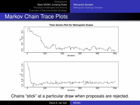
Markov Chain Trace PlotsTime Series Plot for Metropolis Draws
iteration
α
0 100 200 300 400 500
5.0
5.5
6.0
6.5
iteration
β
0 100 200 300 400 500
1.6
1.8
2.0
2.2
2.4
Chains “stick” at a particular draw when proposals are rejected.David A. van Dyk MCMC
uci
BackgroundBasic MCMC Jumping Rules
Practical Challenges and AdviceOverview of Recommended Strategy
Metropolis SamplerMetropolis Hastings Sampler
The Joint Posterior Distribution
4.8 5.0 5.2 5.4 5.61.60
1.65
1.70
1.75
1.80
Scatter Plot of Posterior Distribution
α
β
David A. van Dyk MCMC
uci
BackgroundBasic MCMC Jumping Rules
Practical Challenges and AdviceOverview of Recommended Strategy
Metropolis SamplerMetropolis Hastings Sampler
Marginal Posterior Dist’n of the Normalization
0 20 40 60 80 100
0.0
0.2
0.4
0.6
0.8
1.0
Lag
AC
F
Autocorrelation for alpha Hist of 500 Draws excluding Burn−in
4.8 5.0 5.2 5.4 5.6
01
23
45
4.8 5.0 5.2 5.4 5.6
01
23
45
−− Posterior Density
E(α|Y ) ≈ 5.13, SD(α|Y ) ≈ 0.11, and a 95% CI is (4.92,5.41)
David A. van Dyk MCMC
uci
BackgroundBasic MCMC Jumping Rules
Practical Challenges and AdviceOverview of Recommended Strategy
Metropolis SamplerMetropolis Hastings Sampler
Marginal Posterior Dist’n of Power Law Param
0 20 40 60 80 100
0.0
0.2
0.4
0.6
0.8
1.0
Lag
AC
F
Autocorrelation for beta Hist of 500 Draws excluding Burn−in
1.60 1.65 1.70 1.75 1.80
05
1015
20
1.60 1.65 1.70 1.75 1.80
05
1015
20
−− Posterior Density
E(β|Y ) ≈ 1.71, SD(β|Y ) ≈ 0.03, and a 95% CI is (1.65,1.76)
David A. van Dyk MCMC
uci
BackgroundBasic MCMC Jumping Rules
Practical Challenges and AdviceOverview of Recommended Strategy
Metropolis SamplerMetropolis Hastings Sampler
The Metropolis-Hastings Sampler
A more general Jumping rule:
Draw θ(0) from some starting distribution.
For t = 1,2,3, . . .Sample: θ∗ from Jt (θ
∗|θ(t−1))
Compute: r = p(θ∗|y)/Jt (θ∗|θ(t−1))
p(θ(t−1)|y)/Jt (θ(t−1)|θ∗)
Set: θ(t) =
{θ∗ with probability min(r ,1)
θ(t−1) otherwise
NoteJt may be any jumping rule, it needn’t be symmetric.The updated r corrects for bias in the jumping rule.
David A. van Dyk MCMC
uci
BackgroundBasic MCMC Jumping Rules
Practical Challenges and AdviceOverview of Recommended Strategy
Metropolis SamplerMetropolis Hastings Sampler
The Independence Sampler
Use an approximation to the posterior as the jumping rule:
Jt = Normald (MAP estimate, Curvature-based Variance Matrix).
MAP estimate = argmaxθp(θ|y)
Variance ≈[− ∂2
∂θ · ∂θlog p(θ|Y )
]−1
Note: Jt (θ∗|θ(t−1)) does not depend on θ(t−1).
David A. van Dyk MCMC
uci
BackgroundBasic MCMC Jumping Rules
Practical Challenges and AdviceOverview of Recommended Strategy
Metropolis SamplerMetropolis Hastings Sampler
The Independence Sampler
The Normal Approximation may not be adequate.
theta
f(th
eta)
0 1 2 3 4 5 6 7
0.0
0.1
0.2
0.3
0.4
theta
f(th
eta)
0 1 2 3 4 5 6 7
0.00
0.10
0.20
0.30
We can inflate the variance.We can use a heavy tailed distribution, e.g., lorentzian or t .
David A. van Dyk MCMC
uci
BackgroundBasic MCMC Jumping Rules
Practical Challenges and AdviceOverview of Recommended Strategy
Metropolis SamplerMetropolis Hastings Sampler
Example of Independence Sampler
A simplified model for high-energy spectral analysis.
We can fit (α, β) with a general mode finder (e.g.,Levenberg-Marqardt)Requires coding likelihood (e.g. Cash statistic), specifingstarting values, etc.Base choice of parameter on quality of normal approx.
MLE is invariant to transformations.Variance matrix of transform is computed via delta method.
Can use the jumping rule:Jt = Normal2(MAP est, Curvature-based Variance Matrix).
David A. van Dyk MCMC
uci
BackgroundBasic MCMC Jumping Rules
Practical Challenges and AdviceOverview of Recommended Strategy
Metropolis SamplerMetropolis Hastings Sampler
Markov Chain Trace PlotsTime Series Plot for Metropolis Hastings Draws
iteration
α
0 100 200 300 400 500
5.0
5.5
6.0
6.5
iteration
β
0 100 200 300 400 5001.6
1.8
2.0
2.2
2.4
Very little “sticking” here: acceptance rate is 98.8%.David A. van Dyk MCMC
uci
BackgroundBasic MCMC Jumping Rules
Practical Challenges and AdviceOverview of Recommended Strategy
Metropolis SamplerMetropolis Hastings Sampler
Marginal Posterior Dist’n of the Normalization
0 20 40 60 80 100
0.0
0.2
0.4
0.6
0.8
1.0
Lag
AC
F
Autocorrelation for alpha Hist of 500 Draws excluding Burn−in
4.8 5.0 5.2 5.4 5.6
01
23
45
4.8 5.0 5.2 5.4 5.6
01
23
45
−− Posterior Density
Autocorrelation is essentially zero: nearly independent sample!!
David A. van Dyk MCMC
uci
BackgroundBasic MCMC Jumping Rules
Practical Challenges and AdviceOverview of Recommended Strategy
Metropolis SamplerMetropolis Hastings Sampler
Marginal Posterior Dist’n of Power Law Param
0 20 40 60 80 100
0.0
0.2
0.4
0.6
0.8
1.0
Lag
AC
F
Autocorrelation for beta Hist of 500 Draws excluding Burn−in
1.60 1.65 1.70 1.75 1.80
05
1015
20
1.60 1.65 1.70 1.75 1.80
05
1015
20
−− Posterior Density
This result depends critically on access to a very goodapproximation to the posterior distribution.
David A. van Dyk MCMC
uci
BackgroundBasic MCMC Jumping Rules
Practical Challenges and AdviceOverview of Recommended Strategy
Diagnosing ConvergenceChoosing a Jumping RuleTransformations and Multiple Modes
Outline
1 BackgroundBayesian StatisticsMonte Carlo IntegrationMarkov Chains
3 Practical Challenges and AdviceDiagnosing ConvergenceChoosing a Jumping RuleTransformations and Multiple Modes
4 Overview of Recommended Strategy
David A. van Dyk MCMC
uci
BackgroundBasic MCMC Jumping Rules
Practical Challenges and AdviceOverview of Recommended Strategy
Diagnosing ConvergenceChoosing a Jumping RuleTransformations and Multiple Modes
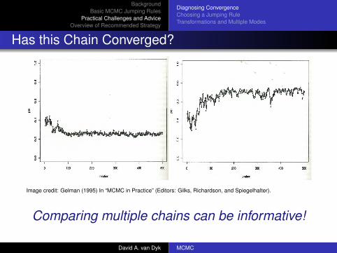
Has this Chain Converged?
Image credit: Gelman (1995) In “MCMC in Practice” (Editors: Gilks, Richardson, and Spiegelhalter).
David A. van Dyk MCMC
uci
BackgroundBasic MCMC Jumping Rules
Practical Challenges and AdviceOverview of Recommended Strategy
Diagnosing ConvergenceChoosing a Jumping RuleTransformations and Multiple Modes
Has this Chain Converged?
Image credit: Gelman (1995) In “MCMC in Practice” (Editors: Gilks, Richardson, and Spiegelhalter).
Comparing multiple chains can be informative!
David A. van Dyk MCMC
uci
BackgroundBasic MCMC Jumping Rules
Practical Challenges and AdviceOverview of Recommended Strategy
Diagnosing ConvergenceChoosing a Jumping RuleTransformations and Multiple Modes
Using Multiple Chains
chain 1
iteration
0 10000 20000
-22
46
logT
chain 2
iteration
0 10000 20000-2
24
6lo
gT
chain 3
iteration
0 10000 20000
-22
46
logT
Compare results of multiple chains to check convergence.Start the chains from distant points in parameter space.Run until they appear to give similar results
... or they find different solutions (multiple modes).
David A. van Dyk MCMC
uci
BackgroundBasic MCMC Jumping Rules
Practical Challenges and AdviceOverview of Recommended Strategy
Diagnosing ConvergenceChoosing a Jumping RuleTransformations and Multiple Modes
The Gelman and Rubin “R hat” Statistic
Consider M chains of length N: {ψnm,n = 1, . . . ,N}.
B =N
M − 1
M∑m−1
(ψ·m − ψ··)2
W =1M
M∑m=1
s2m where s2
m =1
N − 1
N∑n=1
(ψnm − ψ·m)2
Two estimates of Var(ψY ):1 W : underestimate of Var(ψ | Y ) for any finite N.2 var+(ψ | Y ) = N−1
N W + 1N B: overestimate of Var(ψ | Y ).
R =
√var+(ψ | Y )
W↓ 1 as the chains converge.
David A. van Dyk MCMC
uci
BackgroundBasic MCMC Jumping Rules
Practical Challenges and AdviceOverview of Recommended Strategy
Diagnosing ConvergenceChoosing a Jumping RuleTransformations and Multiple Modes
Choice of Jumping Rule with Random Walk Metropolis
Spectral Analysis: effect on burn in of power law parametersigma = 0.005, 0.08, 0.4
iteration
Sam
ple1
0 500 1000 15001.6
1.8
2.0
2.2
2.4
acceptance rate=87.5%Lag one autocorrelation=0.98
iteration
Sam
ple2
0 500 1000 15001.6
1.8
2.0
2.2
2.4
acceptance rate=31.6%Lag one autocorrelation=0.66
iteration
Sam
ple3
0 500 1000 1500
1.4
1.8
2.2
acceptance rate=3.1%Lag one autocorrelation=0.96
David A. van Dyk MCMC
uci
BackgroundBasic MCMC Jumping Rules
Practical Challenges and AdviceOverview of Recommended Strategy
Diagnosing ConvergenceChoosing a Jumping RuleTransformations and Multiple Modes
Higher Acceptance Rate is not Always Better!
500 1000 1500 2000
1.62
1.66
1.70
1.74
sigma = 0.005, 0.08, 0.4
iteration
Sam
ple1
500 1000 1500 20001.60
1.70
1.80
iteration
Sam
ple2
500 1000 1500 20001.60
1.70
1.80
iteration
Sam
ple3
acceptance rate=3.1%
Lag one autocorrelation=0.96
Aim for 20% (vectors) - 40% (scalars) acceptance rateDavid A. van Dyk MCMC
uci
BackgroundBasic MCMC Jumping Rules
Practical Challenges and AdviceOverview of Recommended Strategy
Diagnosing ConvergenceChoosing a Jumping RuleTransformations and Multiple Modes
Statistical Inference and Effective Sample Size
Point Estimate: hn = 1n∑
h(θ(t)) (estimate of E(h(θ)|x)!!)
Variance Estimate: Var(hn) ≈ σ2
n1+ρ1−ρ with (not var(θ)!!)
σ2 = Var(h(θ)) estimated by σ2 = 1n−1
∑nt=1[h(θ(t))− hn]2,
ρ = corr[h(θ(t),h(θ(t−1)
]estimated by
ρ =1
n − 1
∑nt=2[h(θ(t))− hn][h(θ(t−1))− hn]√∑n−1
t=1 [h(θ(t))− hn]2∑n
t=2[h(θ(t))− hn]2
Interval Estimate: hn ± td√
Var(hn) with d = n 1−ρ1+ρ − 1
The effective sample size is n 1−ρ1+ρ .
David A. van Dyk MCMC
uci
BackgroundBasic MCMC Jumping Rules
Practical Challenges and AdviceOverview of Recommended Strategy
Diagnosing ConvergenceChoosing a Jumping RuleTransformations and Multiple Modes
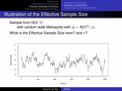
Illustration of the Effective Sample Size
Sample from N(0,1)with random walk Metropolis with Jt = N(θ(t), σ).
What is the Effective Sample Size here? and σ?
0 200 400 600 800 1000
−3
−2
−1
01
23
iteration
Mar
kov
Cha
in
David A. van Dyk MCMC
uci
BackgroundBasic MCMC Jumping Rules
Practical Challenges and AdviceOverview of Recommended Strategy
Diagnosing ConvergenceChoosing a Jumping RuleTransformations and Multiple Modes
Illustration of the Effective Sample Size
What is the Effective Sample Size here? and σ?
0 200 400 600 800 1000
−3
−2
−1
01
23
iteration
Mar
kov
Cha
in
David A. van Dyk MCMC
uci
BackgroundBasic MCMC Jumping Rules
Practical Challenges and AdviceOverview of Recommended Strategy
Diagnosing ConvergenceChoosing a Jumping RuleTransformations and Multiple Modes
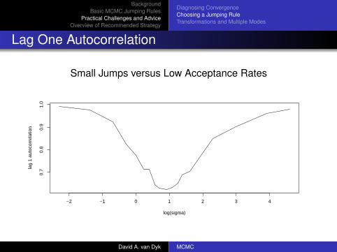
Lag One Autocorrelation
Small Jumps versus Low Acceptance Rates
−2 −1 0 1 2 3 4
0.7
0.8
0.9
1.0
log(sigma)
lag
1 au
toco
rrel
atio
n
David A. van Dyk MCMC
uci
BackgroundBasic MCMC Jumping Rules
Practical Challenges and AdviceOverview of Recommended Strategy
Diagnosing ConvergenceChoosing a Jumping RuleTransformations and Multiple Modes
Effective Sample Size
Balancing the Trade-Off
−2 −1 0 1 2 3 4
050
100
150
200
log(sigma)
effe
ctiv
e sa
mpl
e si
ze
David A. van Dyk MCMC
uci
BackgroundBasic MCMC Jumping Rules
Practical Challenges and AdviceOverview of Recommended Strategy
Diagnosing ConvergenceChoosing a Jumping RuleTransformations and Multiple Modes
Acceptance Rate
Bigger is not always Better!!
−2 −1 0 1 2 3 4
0.0
0.2
0.4
0.6
0.8
1.0
log(sigma)
acce
ptan
ce r
ate
High acceptance rates only come with small steps!!
David A. van Dyk MCMC
uci
BackgroundBasic MCMC Jumping Rules
Practical Challenges and AdviceOverview of Recommended Strategy
Diagnosing ConvergenceChoosing a Jumping RuleTransformations and Multiple Modes
Finding the Optimal Acceptance Rate
−2 −1 0 1 2 3 4
050
100
150
200
log(sigma)
effe
ctiv
e sa
mpl
e si
ze
−2 −1 0 1 2 3 4
0.0
0.2
0.4
0.6
0.8
1.0
log(sigma)
acce
ptan
ce r
ate
David A. van Dyk MCMC
uci
BackgroundBasic MCMC Jumping Rules
Practical Challenges and AdviceOverview of Recommended Strategy
Diagnosing ConvergenceChoosing a Jumping RuleTransformations and Multiple Modes
Random Walk Metropolis with High Correlation
A whole new set of issues arise in higher dimensions...
Tradeoff between high autocorrelation and high rejection rate:more acute with high posterior correlationsmore acute with high dimensional parameter
−3 −2 −1 0 1 2 3
−3
−2
−1
01
23
x
y
David A. van Dyk MCMC
uci
BackgroundBasic MCMC Jumping Rules
Practical Challenges and AdviceOverview of Recommended Strategy
Diagnosing ConvergenceChoosing a Jumping RuleTransformations and Multiple Modes
Random Walk Metropolis with High Correlation
In principle we can use a correlated jumping rule, butthe desired correlation may vary, andis often difficult to compute in advance.
−3 −2 −1 0 1 2 3
−3
−2
−1
01
23
x
y
David A. van Dyk MCMC
uci
BackgroundBasic MCMC Jumping Rules
Practical Challenges and AdviceOverview of Recommended Strategy
Diagnosing ConvergenceChoosing a Jumping RuleTransformations and Multiple Modes
Random Walk Metropolis with High Correlation
What random walk jumping rule would you use here?
−3 −2 −1 0 1 2 3
−3
−2
−1
0
x
y
Remember: you don’t get to see the distribution in advance!
David A. van Dyk MCMC
uci
BackgroundBasic MCMC Jumping Rules
Practical Challenges and AdviceOverview of Recommended Strategy
Diagnosing ConvergenceChoosing a Jumping RuleTransformations and Multiple Modes
Parameters on Different Scales
Random Walk Metropolis for Spectral Analysis:
4.8 5.0 5.2 5.4 5.61.60
1.65
1.70
1.75
1.80
Scatter Plot of Posterior Distribution
α
β
0 20 40 60 80 100
0.0
0.2
0.4
0.6
0.8
1.0
Lag
ACF
Autocorrelation for alpha Hist of 500 Draws excluding Burn−in
4.8 5.0 5.2 5.4 5.6
01
23
45
4.8 5.0 5.2 5.4 5.6
01
23
45
−− Posterior Density
Why is the Mixing SO Poor?!??David A. van Dyk MCMC
uci
BackgroundBasic MCMC Jumping Rules
Practical Challenges and AdviceOverview of Recommended Strategy
Diagnosing ConvergenceChoosing a Jumping RuleTransformations and Multiple Modes
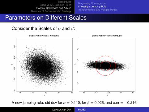
Parameters on Different Scales
Consider the Scales of α and β:
4.8 5.0 5.2 5.4 5.61.60
1.65
1.70
1.75
1.80
Scatter Plot of Posterior Distribution
α
β
4.8 5.0 5.2 5.4 5.6
1.4
1.6
1.8
2.0
Scatter Plot of Posterior Distribution
α
β
A new jumping rule: std dev for α = 0.110, for β = 0.026, and corr = −0.216.
David A. van Dyk MCMC
uci
BackgroundBasic MCMC Jumping Rules
Practical Challenges and AdviceOverview of Recommended Strategy
Diagnosing ConvergenceChoosing a Jumping RuleTransformations and Multiple Modes
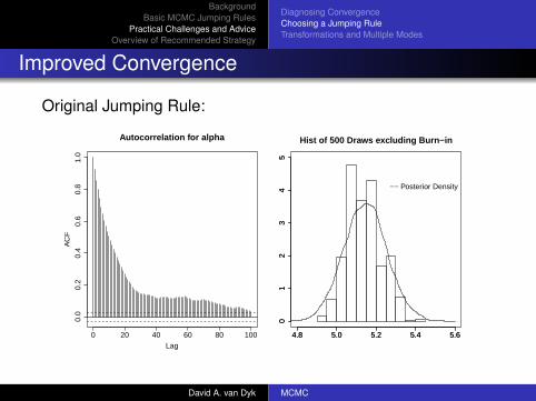
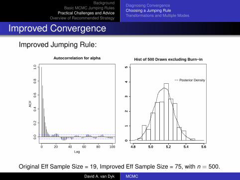
Improved Convergence
Original Jumping Rule:
0 20 40 60 80 100
0.0
0.2
0.4
0.6
0.8
1.0
Lag
AC
F
Autocorrelation for alpha Hist of 500 Draws excluding Burn−in
4.8 5.0 5.2 5.4 5.6
01
23
45
4.8 5.0 5.2 5.4 5.6
01
23
45
−− Posterior Density
David A. van Dyk MCMC
uci
BackgroundBasic MCMC Jumping Rules
Practical Challenges and AdviceOverview of Recommended Strategy
Diagnosing ConvergenceChoosing a Jumping RuleTransformations and Multiple Modes
Improved Convergence
Improved Jumping Rule:
0 20 40 60 80 100
0.0
0.2
0.4
0.6
0.8
1.0
Lag
AC
F
Autocorrelation for alpha Hist of 500 Draws excluding Burn−in
4.8 5.0 5.2 5.4 5.6
01
23
45
4.8 5.0 5.2 5.4 5.6
01
23
45
−− Posterior Density
Original Eff Sample Size = 19, Improved Eff Sample Size = 75, with n = 500.David A. van Dyk MCMC
uci
BackgroundBasic MCMC Jumping Rules
Practical Challenges and AdviceOverview of Recommended Strategy
Diagnosing ConvergenceChoosing a Jumping RuleTransformations and Multiple Modes
Parameters on Different Scales
Strategy: When using
Normal (θ(t−1), kM) or better yettdf(θ
(t−1), kM)
try using the variance-covariance matrix from a standard fittedmodel for M
... at least when there is standard mode-based model-fittingsoftware available.
David A. van Dyk MCMC
uci
BackgroundBasic MCMC Jumping Rules
Practical Challenges and AdviceOverview of Recommended Strategy
Diagnosing ConvergenceChoosing a Jumping RuleTransformations and Multiple Modes
Transforming to Normality
Parameter transformations can greatly improve MCMC.
Recall the Independence Sampler:
theta
f(th
eta)
0 1 2 3 4 5 6 7
0.0
0.1
0.2
0.3
0.4
theta
f(th
eta)
0 1 2 3 4 5 6 7
0.00
0.10
0.20
0.30
The normal approximation is not as good as we might hope...David A. van Dyk MCMC
uci
BackgroundBasic MCMC Jumping Rules
Practical Challenges and AdviceOverview of Recommended Strategy
Diagnosing ConvergenceChoosing a Jumping RuleTransformations and Multiple Modes
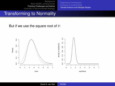
Transforming to Normality
But if we use the square root of θ:
theta
f(th
eta)
0 1 2 3 4 5 6 7
0.0
0.1
0.2
0.3
0.4
sqrt(theta)
dens
ity o
f sqr
t(th
eta)
0 1 2 3 4 5 6 7
0.0
0.2
0.4
0.6
0.8
1.0
1.2
David A. van Dyk MCMC
uci
BackgroundBasic MCMC Jumping Rules
Practical Challenges and AdviceOverview of Recommended Strategy
Diagnosing ConvergenceChoosing a Jumping RuleTransformations and Multiple Modes
Transforming to Normality
And...
theta
f(th
eta)
0 1 2 3 4 5 6 7
0.00
0.10
0.20
0.30
sqrt(theta)
dens
ity o
f sqr
t(th
eta)
0 1 2 3 4 5 6 7
0.0
0.2
0.4
0.6
0.8
The normal approximation is much improved!
David A. van Dyk MCMC
uci
BackgroundBasic MCMC Jumping Rules
Practical Challenges and AdviceOverview of Recommended Strategy
Diagnosing ConvergenceChoosing a Jumping RuleTransformations and Multiple Modes
Transforming to Normality
Working with with Gaussian or symmetric distributions leads tomore efficient Metropolis and Metropolis Hastings Samplers.
General Strategy:Transform to the Real Line.Take the log of positive parameters.If the log is “too strong”, try square root.Probabilities can be transformed via the logit transform:
log(p/(1− p)).
More complex transformations for other quantities.Try out various transformations using an initial MCMC run.Statistical advantages to using normalizing transforms.
David A. van Dyk MCMC
uci
BackgroundBasic MCMC Jumping Rules
Practical Challenges and AdviceOverview of Recommended Strategy
Diagnosing ConvergenceChoosing a Jumping RuleTransformations and Multiple Modes
Removing Linear Correlations
Linear transformations can remove linear correlations
−3 −1 0 1 2 3
−10
−5
05
x
y
−3 −1 0 1 2 3
−0.
6−
0.4
−0.
20.
00.
20.
4
x
y −
3 *
x
David A. van Dyk MCMC
uci
BackgroundBasic MCMC Jumping Rules
Practical Challenges and AdviceOverview of Recommended Strategy
Diagnosing ConvergenceChoosing a Jumping RuleTransformations and Multiple Modes
Removing Linear Correlations
... and can help with non-linear correlations.
0 2 4 6
050
100
150
x
y
0 2 4 6
−30
−20
−10
010
2030
x
y −
18
* x
David A. van Dyk MCMC
uci
BackgroundBasic MCMC Jumping Rules
Practical Challenges and AdviceOverview of Recommended Strategy
Diagnosing ConvergenceChoosing a Jumping RuleTransformations and Multiple Modes
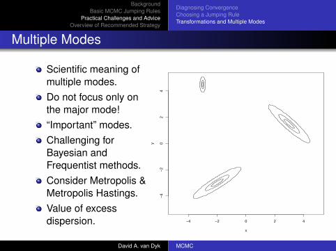
Multiple Modes
Scientific meaning ofmultiple modes.Do not focus only onthe major mode!“Important” modes.Challenging forBayesian andFrequentist methods.Consider Metropolis &Metropolis Hastings.Value of excessdispersion. −4 −2 0 2 4
−4
−2
02
4
x
y
David A. van Dyk MCMC
uci
BackgroundBasic MCMC Jumping Rules
Practical Challenges and AdviceOverview of Recommended Strategy
Diagnosing ConvergenceChoosing a Jumping RuleTransformations and Multiple Modes
Multiple Modes
1 Use a mode finder to “map out” the posterior distribution.1 Design a jumping rule that accounts for all of the modes.2 Run separate chains for each mode.
2 Use on of several sophisticated methods tailored formultiple modes.
1 Adaptive Metropolis Hastings. Jumping rule adapts whennew modes are found (van Dyk & Park, MCMC Hdbk 2011).
2 Parallel Tempering.3 Many other specialized methods.
David A. van Dyk MCMC
uci
BackgroundBasic MCMC Jumping Rules
Practical Challenges and AdviceOverview of Recommended Strategy
Outline
1 BackgroundBayesian StatisticsMonte Carlo IntegrationMarkov Chains
3 Practical Challenges and AdviceDiagnosing ConvergenceChoosing a Jumping RuleTransformations and Multiple Modes
4 Overview of Recommended Strategy
David A. van Dyk MCMC
uci
BackgroundBasic MCMC Jumping Rules
Practical Challenges and AdviceOverview of Recommended Strategy
Overview of Recommended Strategy
(Adopted from Bayesian Data Analysis, Section 11.10, Gelmanet al. (2005), Second Edition)
1 Start with a crude approximation to the posteriordistribution, perhaps using a mode finder.
2 Simulate directly, avoiding MCMC, if possible.3 If necessary use MCMC with one parameter at a time
updating or updating parameters in batches:Two-Step Gibbs Sampler:
Step 1: Sample θ(t) dist∼ p(θ | φ(t−1),Y )
Step 2: Sample φ(t) dist∼ p(φ | θ(t),Y )
4 Use Gibbs draws for closed form complete conditionals.
David A. van Dyk MCMC
uci
BackgroundBasic MCMC Jumping Rules
Practical Challenges and AdviceOverview of Recommended Strategy
Overview of Recommended Strategy- Con’t
5 Use metropolis jumps if complete conditional is not inclosed form. Tune variance of jumping distribution so thatacceptance rates are near 20% (for vector updates) or40% (for single parameter updates).
6 To improve convergence, use transformations so thatparameters are approximately independent.
7 Check for convergence using multiple chains.8 Compare inference based on crude approximation and
MCMC. If they are not similar, check for errors beforebelieving the results of the MCMC.