MNRAS 492, 4043–4057 (2020) doi:10.1093/mnras/staa073Advance Access publication 2020 January 24

Markov Chain Monte Carlo population synthesis of single radio pulsarsin the Galaxy

Marek Cieslar ,1‹ Tomasz Bulik2 and Stefan Osłowski 3,4,5

1Nicolaus Copernicus Astronomical Center, Polish Academy of Sciences, Bartycka 18, PL-00-716 Warsaw, Poland2Astronomical Observatory, University of Warsaw, Al Ujazdowskie 4, PL-00-478 Warsaw, Poland3Centre for Astrophysics and Supercomputing, Swinburne University of Technology, Hawthorn, VIC 3122, Australia4Fakultat fur Physik, Universitat Bielefeld, Postfach 100131, D-33501 Bielefeld, Germany5Max-Planck-Intitut fur Radioastronomie, Auf dem Hugel 69, D-53121 Bonn, Germany

Accepted 2020 January 8. Received 2020 January 5; in original form 2018 March 6

ABSTRACTWe present a model of evolution of solitary neutron stars, including spin parameters, magneticfield decay, motion in the Galactic potential, and birth inside spiral arms. We use twoparametrizations of the radio-luminosity law and model the radio selection effects. Dispersionmeasure is estimated from the recent model of free electron distribution in the Galaxy(YMW16). Model parameters are optimized using the Markov Chain Monte Carlo technique.The preferred model has a short decay scale of the magnetic field of 4.27+0.4

−0.38 Myr. However,it has non-negligible correlation with parameters describing the pulsar radio luminosity. Basedon the best-fitting model, we predict that the Square Kilometre Array surveys will increasethe population of known single radio pulsars by between 23 and 137 per cent. The INDRI codeused for simulations is publicly available to facilitate future population synthesis efforts.

Key words: methods: numerical – stars: neutron – pulsars: general – stars: statistics.

1 IN T RO D U C T I O N

Evolution of neutron stars (NS) has been a subject of intense studiesin the past. These objects are primarily observed as radio pulsars butcan also be seen in other bands like the X-rays, gamma rays as wellas in the optical range. There have been numerous efforts to modelthe radio population. Most notably the works of Narayan & Ostriker(1990), Faucher-Giguere & Kaspi (2006), Gonthier et al. (2007)then Kiel et al. (2008), Kiel & Hurley (2009), Osłowski et al. (2011)and in recent years Levin et al. (2013), Gullon et al. (2014), andBates et al. (2014). For an in-depth review of population synthesisefforts, see Popov & Prokhorov (2007) and Lorimer (2011).

We base our motivation to revisit the radio population of pulsarson the improved model of the electron density in the Galaxy Yao,Manchester & Wang (2017), and the availability of Markov ChainMonte Carlo (MCMC) to explore the multidimensional parameterspace due to the extended computational power. We restrict ouranalysis to the evolution of the single pulsars from their birth ina supernova (SN) explosion to the moment they no longer can bedetected in the radio waveband. We do not consider binary evolutionand interactions therefore treatment of millisecond pulsars is beyondthe scope of this paper. We do not simulate the full stellar and binaryevolution that leads to formation of pulsars, such as was done byKiel et al. (2008), Kiel & Hurley (2009), and Osłowski et al. (2011)and therefore we start with pulsars progenitor distribution as an

� E-mail: mcie@camk.edu.pl

input parameter to the simulation. We provide the INDRI sourcecode1 with an intent that one can fully reproduce our results uponaccess to a small cluster,2 expand the scope of the simulation, usedifferent data cuts or jump-start further development.

The paper is arranged as follows: in Section 2, we explain theGalactic model, the kinematics of pulsar population, the evolutionof the pulsars period, and the magnetic field, luminosity models, theselection effects, as well as the mathematical representation of themodel, in Section 3, we describe the construction of the likelihoodof the model upon comparison with survey data and describe theimplementation of the Mertropolis–Hasting MCMC method, andin Section 4 we present the results obtained in the simulation, wediscuss them in the Section 5, and we summarize in Section 6.

2 TH E MO D EL

There are two broadly independent parts that are needed to describethe evolution of NSs. The first part is connected with the dynamicalevolution of NSs in the gravitational potential of the Milky Way,and the second describes the intrinsic evolution in time of eachNS as a radio pulsar. The model is roughly following the onepresented by Faucher-Giguere & Kaspi (2006). In the following

1The code can be obtained from the GitHub repository, http://github.com/cieslar/Indri2At the time of writing, we define such machine as an approximately 200-cores cluster.

C© 2020 The Author(s)Published by Oxford University Press on behalf of the Royal Astronomical Society

Dow

nloaded from https://academ

ic.oup.com/m

nras/article-abstract/492/3/4043/5715465 by Swinburne Library user on 20 M

arch 2020

4044 M. Cieslar, T. Bulik and S. Osłowski

sectio,n we concentrate on the differences between our model andFaucher-Giguere & Kaspi (2006), while the identical componentsare presented in Appendix A. We assume that the pulsars birth timehas a uniform distribution. We model the evolution over a periodof tmax = 50 Myr. It is important to note that the characteristic ageτ = P/2P can reach much higher values than tmax because of themagnetic field decay (see discussion in 5.1.7).

2.1 The Milky Way

2.1.1 The equation of motion-integration method

We use the Verlet method (Verlet 1967) to propagate pulsars throughthe Galactic potential. Following a Monte Carlo experiment (simu-lated motion of few millions of random pulsars), we found that themaximal time-step cannot exceed dtmax = 0.1 Myr in order to limitthe loss of the total energy to 1 per cent due to the numerical errors.The actual time-step dtact is lower then dtmax and it is equal to:

dtact = tagetage

dtmax+ 1

(1)

We discard pulsars which are more than 35 kpc away from theGalactic centre at the end of the simulation.

2.2 The neutron star physics

We assume constant values for the radius (RNS = 10 km), the mass(MNS = 1.4 M�), and the moment of inertia (INS = 1045 g cm2) ofeach NS.

2.2.1 The magnetic field decay

Following Osłowski et al. (2011), we assume that the magneticfield decays due to the Ohmic dissipation. For recent advanced, werefer to the work of Igoshev & Popov (2015), though we simplifythe time dependence of the decay to an exponential function. Thedecay model is parametrized by the time-scale �:

B(t) = (Binit − Bmin) exp

(−t

�

)+ Bmin (2)

To be consistent with our previous work Osłowski et al. (2011), andwith Kiel et al. (2008), we use the minimum value of the magneticfield given by Zhang & Kojima (2006). We draw it from a log-uniform distribution:

107 G < Bmin < 108 G (3)

The results do not depend on the choice of Bmin since the pulsarswith such small magnetic field are not included in the comparisonsample as they no longer emit in radio.

2.2.2 The evolution in time

The boundary conditions for the pulsars evolution are their initialand final magnetic field strength Binit, Bmin, as well the spin periodat birth Pinit. To obtain a set of values P and B at the time tage weintegrate the radiating magnetic dipole (equation A9) by supplyingit with the magnetic field decay (equation 2):

P (tage) = 1

η

√2∫ tage

0(B2(t)dt) + P 2

init (4)

where η � 3.2 × 1019 G s−1/2.

P (tage) =(

1

η2

((Binit − Bmin)2

(1 − e− 2tage

�

)� + 4Bmin(Binit − Bmin)

(1 − e− tage

�

)� + 2B2

mintage

)+ P 2

init

) 12

(5)

We obtain P by inserting P(tage) in equation (A9).

2.3 Radio properties

2.3.1 The phenomenological radio luminosities

Since the first pulsar detection (Hewish et al. 1969), their radioemission process is still in debate (Beskin et al. 2015). In our work,we assume a simple model of pair creation. Though, due to thephenomenological treatment of the luminosity it does not add anyconstraints, it is of significance only while considering the deathlines (see Section 2.3.2). In this paper, we use two different a prioriassumptions about the radio luminosity.

2.3.1.1 The two-parameter power law. The general approach todescribe the phenomenological relation between the P period,period derivative P , and the radio luminosity Lν at frequency ν

is a power law with two parameters α, β, and a scaling factor γ , seee.g. Faucher-Giguere & Kaspi (2006) and Bates et al. (2014):

L400,p−l = γP αPβ

15 mJy × kpc2, (6)

for the observational frequency ν = 400 MHz.

2.3.1.2 The rotational energy power law A more restricted modelis the one in which the luminosity is proportional to the rotationalenergy loss, see e.g. Narayan & Ostriker (1990):

Lrot ≡ −Erot = 4π2P

P 3, (7)

L400,rot = γ

(P

13

15P−1

)κ

mJy × kpc2. (8)

We include the correction Lcorr proposed by Faucher-Giguere &Kaspi (2006) and adopted by Bates et al. (2014) to both radio-fluxlaws (equations 6 and 7):

log L400 = log(L400,rot/p−l) + Lcorr (9)

The Lcorr is randomly drawn from the normal distribution withσ corr = 0.8 and accounts for spread of observed population aroundany parametric models of radio luminosity. We assume that the radiospectrum can be described by a power law:

Lν = Lν0

(ν

ν0

)αsp

(10)

with the spectral index αsp = −1.4 (Maron et al. 2000). Pulsaremission is highly anisotropic. In order to model the geometry ofthe beam from a pulsar we incorporate the beaming factor followingTauris & Manchester (1998). For a pulsar with the period P, wecalculate the beaming fraction f(P) in per cent:

f (P ) = 9 ×(

logP

10 s

)2

+ 3 (11)

and determine the visibility of each pulsar assuming randomorientation.

MNRAS 492, 4043–4057 (2020)

Dow

nloaded from https://academ

ic.oup.com/m

nras/article-abstract/492/3/4043/5715465 by Swinburne Library user on 20 M

arch 2020

MCMC population synthesis of pulsars 4045

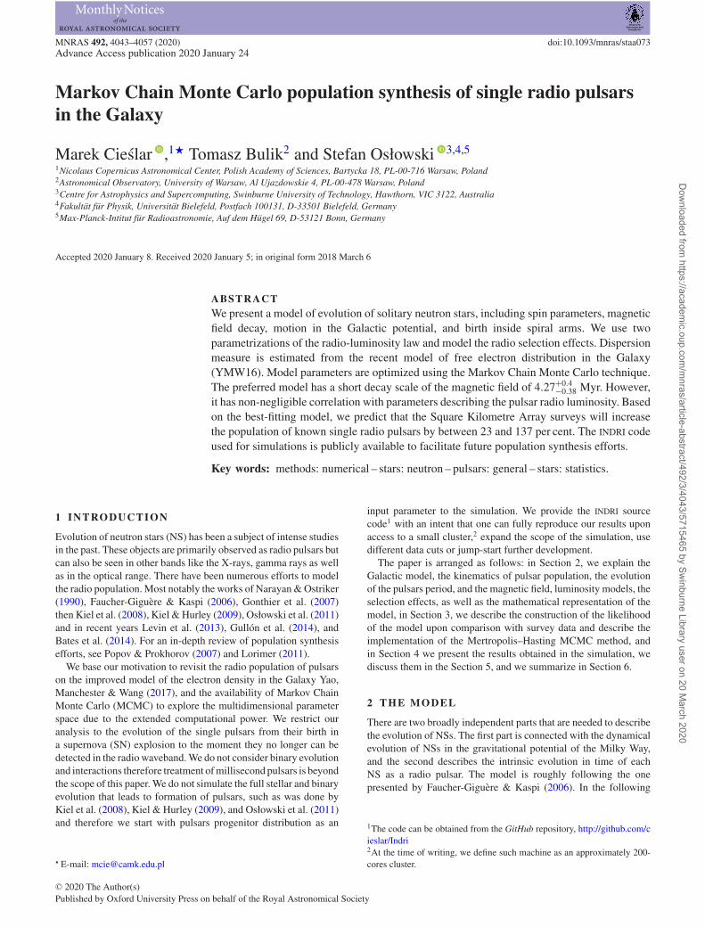
Figure 1. Death area (DArea) – the effective emission probability. Soliddark lines – canonical death lines (DLine) by Rudak & Ritter (1994). Greypoints – subselection of ATNF catalogue used in the simulation.

2.3.2 Death lines–death areas

In the canonical emission process (see Pacini 1967; Gold 1968),the radio waves are emitted due to the e± pair creation and theiracceleration and cascade creation in the presence of strong magneticfield. The pulsars radio emission process stops when the processescannot be sustained (Rudak & Ritter 1994). These so-called deathlines are defined as:

log P = 3.29 × log P − 16.55, (12)

log P = 0.92 × log P − 18.65. (13)

Any pulsar crossing them during its evolution is considered radioinactive. However, such model contradicts the observations as anumber of pulsars lie below these lines. This discrepancy can beattributed to the fact that death lines are devised for a specificstructural model and parameters of the NS. Similarly to Arzouma-nian, Chernoff & Cordes (2002), we propose a phenomenologicalfunction to smooth the death lines into a continuous death area (seeFig. 1). We propose a following formula:

DArea(P , P ) = 1

πarctan

(log P − DLine(log P )

�

)+ 0.5. (14)

The value of � parameter is set to 0.2 in order for the probabilityof radio activity to change in the range of d log P ∼ 1.

2.3.3 The dispersion measure

We compute the dispersion measure (DM) for each pulsar in themodel population using the new and updated model of the electrondensity in the Milky Way (Yao et al. 2017, YMW16). The INDRI codecan also use the NE2001 model (see Cordes & Lazio 2002, 2003).

2.4 The computations

2.4.1 The mathematical representation

To mathematically represent the model, we construct pulsar densityin a 3d space and smooth it with a Gaussian kernel. This comparisonspace is spanned by the period P, the period derivative P , and the

flux at 1400 MHz, S1400 (shortened to S hereafter). The Gaussianaveraged number of pulsars at a particular point (specified by indicesk, l, m) of the comparison space logPk − logPl − logSm is expressedby:

ρklm =PSR∑b

1

(2πσcs)32

exp

(− (logPb − logPk)2

2σ 2cs

)

· exp

(−(logPb − logPk

)2

2σ 2cs

)exp

(− (logSb − logSk)2

2σ 2cs

),

(15)

where σ cs is equal to 0.2. The particular value of the meta-parameterσ cs has been heuristically chosen based on the behaviour of themodel. Too low and the algorithm (described in Section 3.2) wouldnever converge. Too large and the model would reflect and find onlythe maximum of the 3D distribution in the log P − log P − log S

space. To normalize the ρklm, we use the sum R over all relevantpoints (located near observations):

R =∑l,k,m

ρklm (16)

And then, construct the normalized, Gaussian averaged, pulsardensity:

ρklm = 1

Rρklm (17)

For the ease of notation we re-index the k, l, m indices with single i-index traversing all combinations of the k, l, m set. So that ρi :=ρklm

represents a distinct point in the logPk − logPl − logSm space.

2.4.2 The performance of the evolutionary code

We have found that the main performance bottleneck in ourcomputations is the evaluation of the DM in the YMW16 model.The code provided by Yao et al. (2017)3 was not intended to be apart of a high-performance computation and thus, we faced a choice.We could scale back the computation and abandon the Monte Carloapproach of the parameter search. Or we might make the Galacticpart of the model static losing the ability to test SN kicks and initialposition assumptions. We chose the latter option. The resultingalgorithm is executed in two steps:

(i) We simulate the motion in the Galactic potential (as describedin Section 2.1). The goal is to have one million NS that are in thesky window of the Parkes Survey. This number of pulsars is chosenfor practical, computational reasons. We call this set of stars thegeometrical reference population.

(ii) We take the geometrical reference population (the age, DM,and distance) and use it as an input for physical computation(Section 2.2). We use each NS from the geometrical referencepopulation five times, i.e. we place five different model pulsarsat each location, so that they have the same position in the sky andthe same DM. The evolution computations finish with the radio-visibility test (Section 2.3). We check whether the pulsar is beamingtowards Earth and if it is emitting radio waves according to thedeath area criteria. If both conditions are satisfied we compute theluminosity L400 and the detected flux on Earth. To finish the testwe check if the pulsars flux is higher then his minimal detectable

3We use the version 1.2.2 from www.xao.ac.cn/ymw16/

MNRAS 492, 4043–4057 (2020)

Dow

nloaded from https://academ

ic.oup.com/m

nras/article-abstract/492/3/4043/5715465 by Swinburne Library user on 20 M

arch 2020

4046 M. Cieslar, T. Bulik and S. Osłowski

flux. The population that satisfies the radio-visibility test is calledthe model population. This step ends with the computations of thelikelihood statistic in the comparison space (see Section 3.1.2).

The first step is done only once, while the second step is used forthe intensive Monte Carlo computations described in the followingsection. Such scheme allows us to investigate the model by usinga population of five million pulsars. We note that should theYMW16 model be rewritten in computationally efficient way, itwould be possible to carry out the simulation with the inclusionof a parametrization of the initial positions, the SN kicks, and theGalactic potential.

3 C OMPARISON W ITH OBSERVATIONS

3.1 The observations

For the verification, we compare our model with a subset of the Aus-tralia Telescope National Facility Pulsar Catalogue4 (Manchesteret al. 2005). We perform the following cuts to select an unbiasedsample of pulsars:

(i) we preselect single pulsars with measured necessary parame-ters (P, P , S1400, l, b, and DM),

(ii) we choose only the pulsars that have been observed by theParkes Multibeam Survey (Manchester et al. 2001),

(iii) since we focus on the evolution of single pulsars we neglectthe potentially recycled ones by requiring the inferred surfacemagnetic field to be greater then 1010 G.

With these cuts we obtained a subset of 969 pulsars. In order to beconsistent, we perform the second and third cuts as throughout themodel population as well.

3.1.1 The comparison between model and observations

The pulsars density described in Section 2.4.1 can be expressed forboth the model (ρ → m) or the observations (ρ → o). For a givenith point of the comparison space, we compare the model mi pulsardensity with the observed oi pulsar density. Using the central limittheorem, we assume that the probability that the measured densityoi has its value given the model density mi is described by a normaldistribution:

Pi(θ ) = P(mi(θ ), oi) = 1√2π

exp

(− (mi(θ ) − oi)2

2

)(18)

where we denoted the model parameters as θ . For numerical reasons,it more convenient to work with the logarithm of the probabilityPi:

lnPi(θ) = − ln(√

2π) − (mi(θ ) − oi)2

2(19)

3.1.2 Likelihood

In order to find optimal parameters for the model, we use thelikelihood statistic. In general, the likelihood L of n independentvariables x1, . . . , xn drawn from an unknown probability distributionparametrized by θ is expressed by a joint probability function f:

L(θ ; x1, . . . , xn) = f (x1, x2, . . . , xn | θ ) (20)

4Version 1.54, http://www.atnf.csiro.au/research/pulsar/psrcat

Table 1. The constraints of the parameters. The Space columnindicates whether the parameters axis is linear or logarithmic. Italso correspond to the parameters jump probability distribution– normal or lognormal, respectively. The α, β, and κ parametersare dimensionless.

Parameter Min value Max value Space

α −2. 2. 1β −0.5 1. 1κ 0.2 1.4 1γ mJy 10−4 104 log� Myr 100 102 logBinit G 1012 1013 logσBinit G 100.25 100.7 logPinit s 0.01 0.6 1σPinit s 0.01 0.6 1

The joint probability function f is a product of probability functionsg:

f (x1, x2, . . . , xn | θ ) =n∏

i=1

g(xi | θ ). (21)

In our case, due to the finite number of points in the comparisonspace, the independent variables x1, . . . , xn are represented by thepoints mi (as defined in the Sections 2.4.1 and 3.1.1). The probabilitydensity function g is represented by P (equation 18):

L(θ ) =∏i∈�

Pi(θ ) (22)

where � denotes the set of points at which we calculate thepulsars density ρ i. For our computation we use the logarithm ofthe likelihood:

lnL(θ ) =∑i∈�

lnPi(θ ) (23)

3.2 Markov Chain Monte Carlo

To find the most probable parameters of the model, we use theMCMC technique. For the discussion of this widely used and estab-lished concept, we refer to the works of Tarantola (2005), MacKay(2003), or Sharma (2017). In our case, we use the Metropolis–Hastings random walk (Hastings 1970) approach to construct chainsof likelihood values. At the start of each chain, the parameter vectorθ is randomly drawn from the whole available parameters subspace(see Table 1 and Section 4 for parameters definitions) using a flatdistribution in each dimension. During the random walk phase, thenew set of parameters is drawn according to the normal probabilitydistribution centred at the old set of parameters. The drawing isdone independently for each ith parameter:

P(θ i

n, θip

)= 1√

2πσ 2θi

exp

⎛⎜⎝−(θ i

n − θ ip

)2

2σ 2θi

⎞⎟⎠ (24)

where the σθi is set to a 13 rd of the parameter interval (for the

interval description see Table 1). To draw parameters whose initialdistribution is lognormal, we replace the value of the parameterwith its logarithm in equation (24). If the newly drawn param-eter is outside of bounds the procedure is repeated. Followingthe methodology presented by Mosegaard & Tarantola (1995),we use the likelihood-modified step function to decide if thechain will move to the next location in the Metropolis–Hastings

MNRAS 492, 4043–4057 (2020)

Dow

nloaded from https://academ

ic.oup.com/m

nras/article-abstract/492/3/4043/5715465 by Swinburne Library user on 20 M

arch 2020

MCMC population synthesis of pulsars 4047

algorithm:

Rpn = L(θn)

L(θp)(25)

where p and n denote the previous and next set of parameters θ ofa given step. If Rpn � 1, the jump is certain. If it is Rpn < 1, thena jump to next set of parameters is done with the probability equalto Rpn. The calculations are repeated until the distribution of chainend-points becomes subjectively stable.

3.2.1 Optimization and verification of the MCMC

We have learnt that some of the Markov Chains converge on themaximum too slowly or not at all (should they be initially locatedtoo far from the extrema in the parameter space). This is well known,general problem of MCMC methods. It differs between algorithmsand techniques and can be, depending on the technique, minimizedto some extent. Instead of implementing more sophisticated method(see Gilks, Best & Tan 1995; Foreman-Mackey et al. 2013), we didtwo kinds of simulations. A general one, with a broad step-sizeto pinpoint the general area of the maximum of the likelihood (asdescribed in previous subsection). And a second one, starting froma single point in the vicinity of the maximum of likelihood with fourtimes smaller step-size (a 1

12 th of the parameter interval describedin Table 1). We have run 1000 chains, each 5000-links long. Weconfirmed that the chains reach stability by computing the integratedautocorrelation time IAT5 (see Goodman & Weare 2010). Themaximum IAT values, among all marginal parameters distributions,were 279 and 176 links for the power-law and rotational models,respectively.

4 R ESULTS

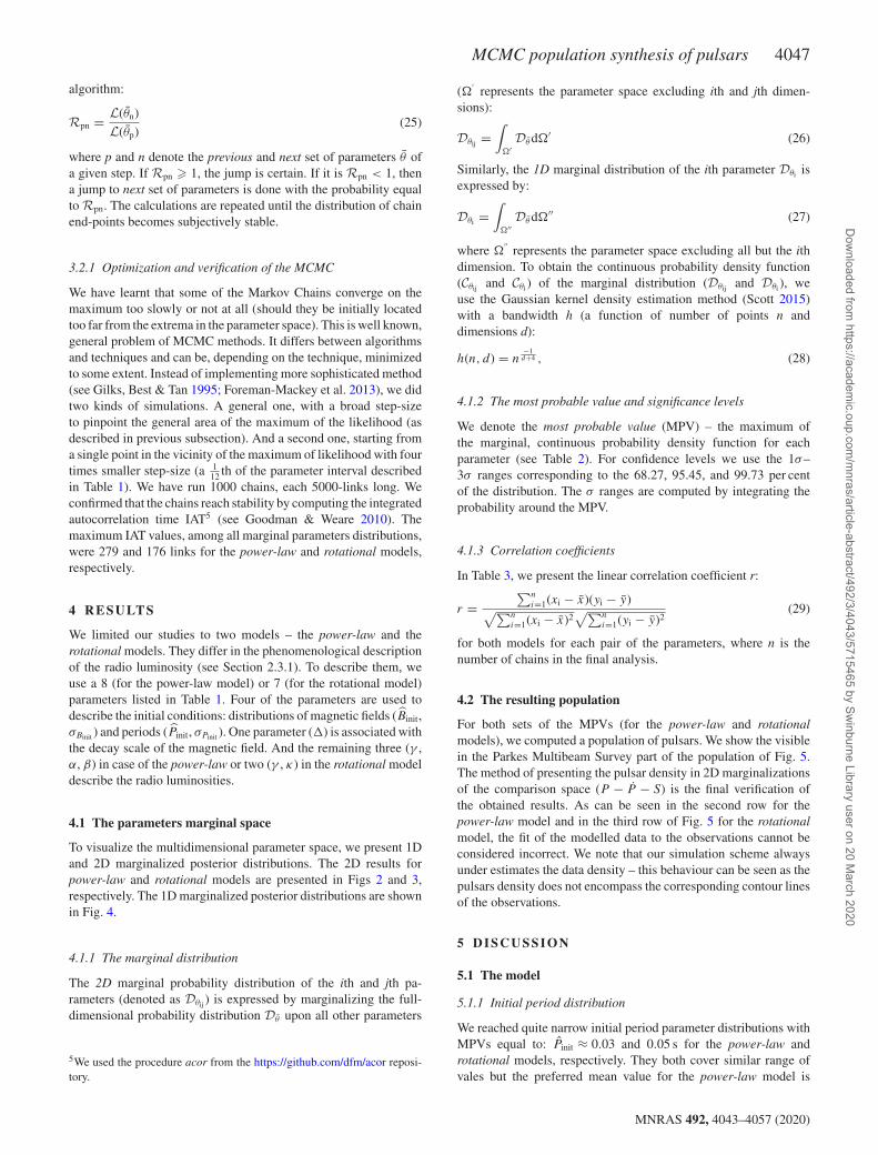
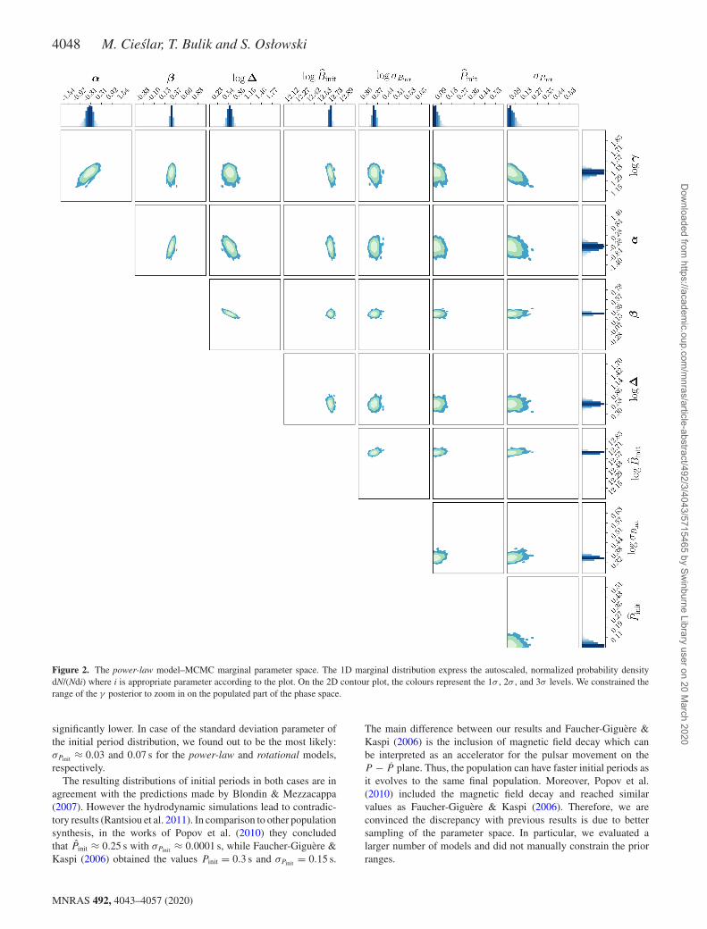
We limited our studies to two models – the power-law and therotational models. They differ in the phenomenological descriptionof the radio luminosity (see Section 2.3.1). To describe them, weuse a 8 (for the power-law model) or 7 (for the rotational model)parameters listed in Table 1. Four of the parameters are used todescribe the initial conditions: distributions of magnetic fields (Binit,σBinit ) and periods (Pinit, σPinit ). One parameter (�) is associated withthe decay scale of the magnetic field. And the remaining three (γ ,α, β) in case of the power-law or two (γ , κ) in the rotational modeldescribe the radio luminosities.

4.1 The parameters marginal space

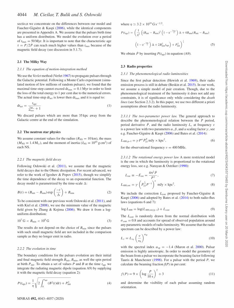
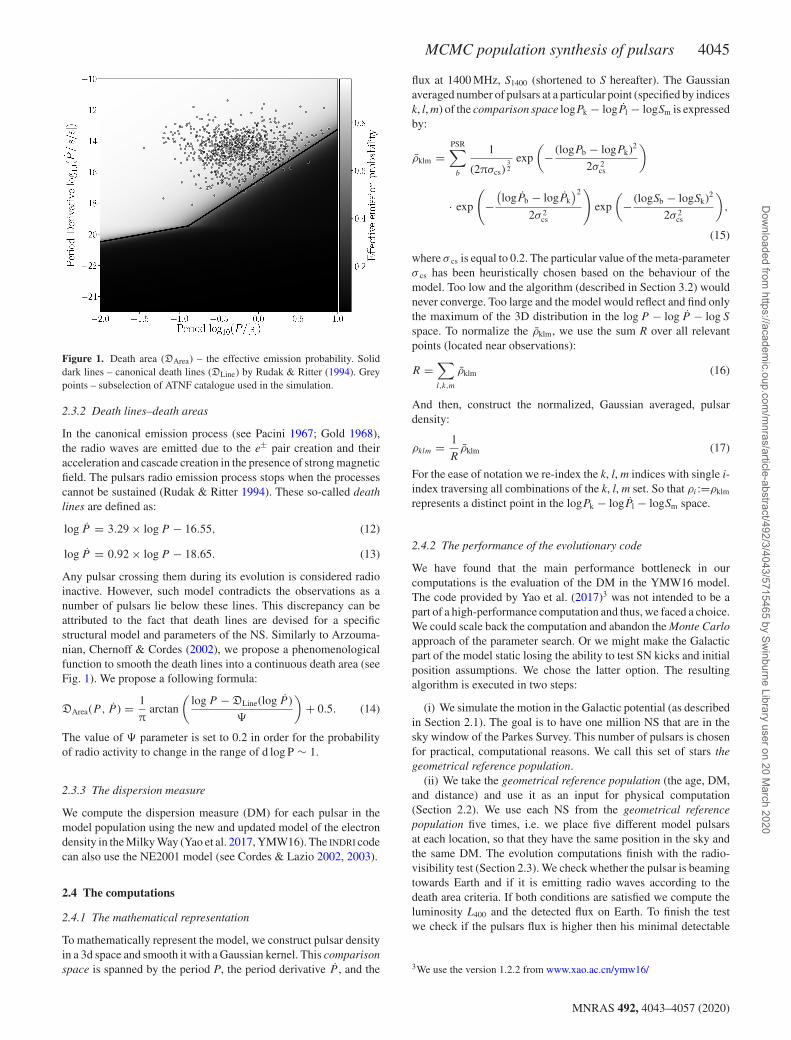
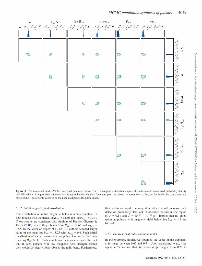
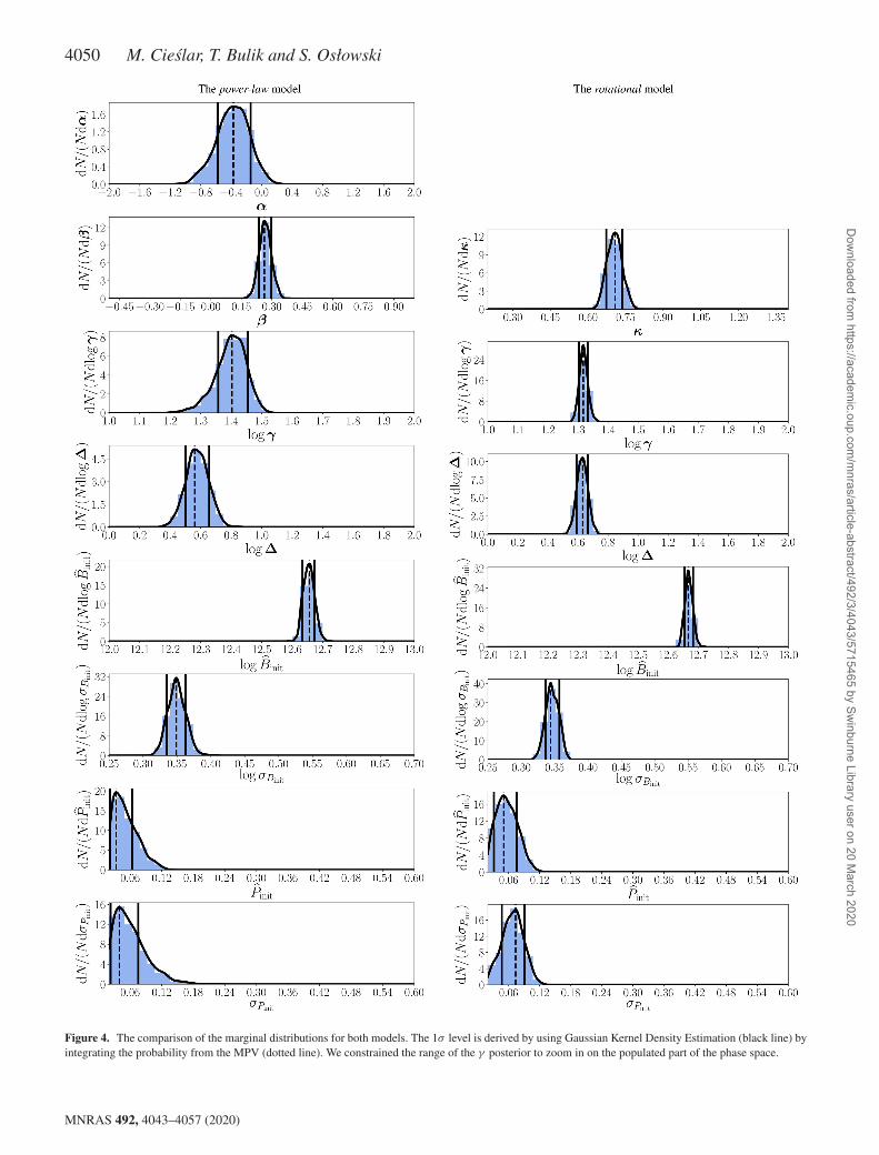
To visualize the multidimensional parameter space, we present 1Dand 2D marginalized posterior distributions. The 2D results forpower-law and rotational models are presented in Figs 2 and 3,respectively. The 1D marginalized posterior distributions are shownin Fig. 4.

4.1.1 The marginal distribution

The 2D marginal probability distribution of the ith and jth pa-rameters (denoted as Dθij ) is expressed by marginalizing the full-dimensional probability distribution Dθ upon all other parameters

5We used the procedure acor from the https://github.com/dfm/acor reposi-tory.

(�′

represents the parameter space excluding ith and jth dimen-sions):

Dθij =∫

�′Dθ d�′ (26)

Similarly, the 1D marginal distribution of the ith parameter Dθi isexpressed by:

Dθi =∫

�′′Dθ d�′′ (27)

where �′′

represents the parameter space excluding all but the ithdimension. To obtain the continuous probability density function(Cθij and Cθi ) of the marginal distribution (Dθij and Dθi ), weuse the Gaussian kernel density estimation method (Scott 2015)with a bandwidth h (a function of number of points n anddimensions d):

h(n, d) = n−1d+4 , (28)

4.1.2 The most probable value and significance levels

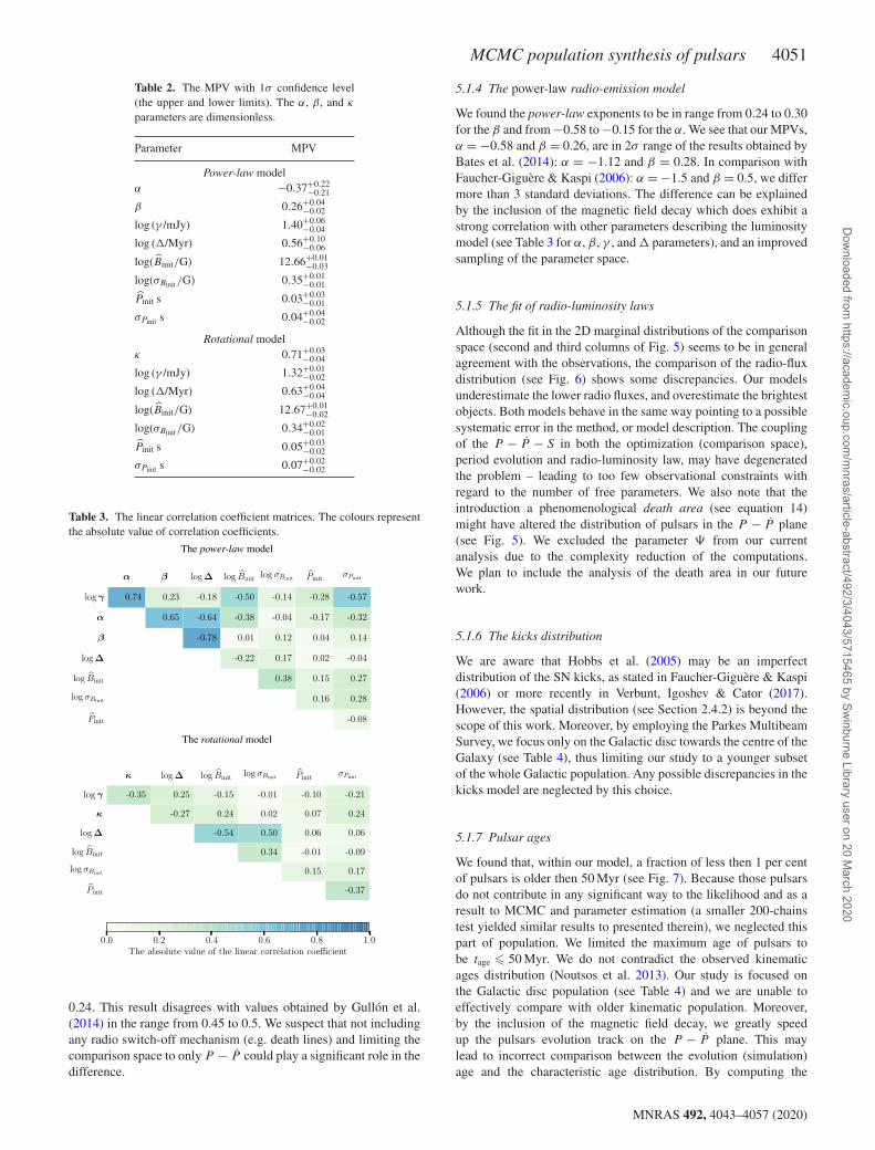
We denote the most probable value (MPV) – the maximum ofthe marginal, continuous probability density function for eachparameter (see Table 2). For confidence levels we use the 1σ–3σ ranges corresponding to the 68.27, 95.45, and 99.73 per centof the distribution. The σ ranges are computed by integrating theprobability around the MPV.

4.1.3 Correlation coefficients

In Table 3, we present the linear correlation coefficient r:

r =∑n

i=1(xi − x)(yi − y)√∑n

i=1(xi − x)2√∑n

i=1(yi − y)2(29)

for both models for each pair of the parameters, where n is thenumber of chains in the final analysis.

4.2 The resulting population

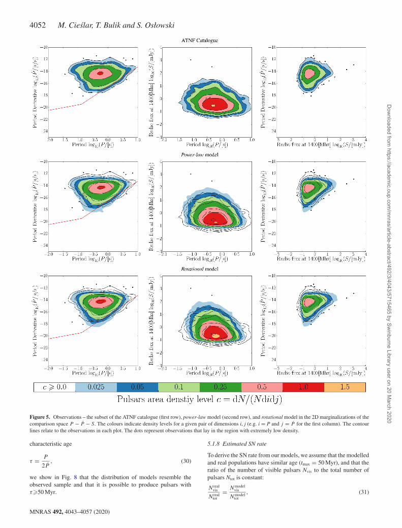
For both sets of the MPVs (for the power-law and rotationalmodels), we computed a population of pulsars. We show the visiblein the Parkes Multibeam Survey part of the population of Fig. 5.The method of presenting the pulsar density in 2D marginalizationsof the comparison space (P − P − S) is the final verification ofthe obtained results. As can be seen in the second row for thepower-law model and in the third row of Fig. 5 for the rotationalmodel, the fit of the modelled data to the observations cannot beconsidered incorrect. We note that our simulation scheme alwaysunder estimates the data density – this behaviour can be seen as thepulsars density does not encompass the corresponding contour linesof the observations.

5 D ISCUSSION

5.1 The model

5.1.1 Initial period distribution

We reached quite narrow initial period parameter distributions withMPVs equal to: Pinit ≈ 0.03 and 0.05 s for the power-law androtational models, respectively. They both cover similar range ofvales but the preferred mean value for the power-law model is

MNRAS 492, 4043–4057 (2020)

Dow

nloaded from https://academ

ic.oup.com/m

nras/article-abstract/492/3/4043/5715465 by Swinburne Library user on 20 M

arch 2020

4048 M. Cieslar, T. Bulik and S. Osłowski

Figure 2. The power-law model–MCMC marginal parameter space. The 1D marginal distribution express the autoscaled, normalized probability densitydN/(Ndi) where i is appropriate parameter according to the plot. On the 2D contour plot, the colours represent the 1σ , 2σ , and 3σ levels. We constrained therange of the γ posterior to zoom in on the populated part of the phase space.

significantly lower. In case of the standard deviation parameter ofthe initial period distribution, we found out to be the most likely:σPinit ≈ 0.03 and 0.07 s for the power-law and rotational models,respectively.

The resulting distributions of initial periods in both cases are inagreement with the predictions made by Blondin & Mezzacappa(2007). However the hydrodynamic simulations lead to contradic-tory results (Rantsiou et al. 2011). In comparison to other populationsynthesis, in the works of Popov et al. (2010) they concludedthat Pinit ≈ 0.25 s with σPinit ≈ 0.0001 s, while Faucher-Giguere &Kaspi (2006) obtained the values Pinit = 0.3 s and σPinit = 0.15 s.

The main difference between our results and Faucher-Giguere &Kaspi (2006) is the inclusion of magnetic field decay which canbe interpreted as an accelerator for the pulsar movement on theP − P plane. Thus, the population can have faster initial periods asit evolves to the same final population. Moreover, Popov et al.(2010) included the magnetic field decay and reached similarvalues as Faucher-Giguere & Kaspi (2006). Therefore, we areconvinced the discrepancy with previous results is due to bettersampling of the parameter space. In particular, we evaluated alarger number of models and did not manually constrain the priorranges.

MNRAS 492, 4043–4057 (2020)

Dow

nloaded from https://academ

ic.oup.com/m

nras/article-abstract/492/3/4043/5715465 by Swinburne Library user on 20 M

arch 2020

MCMC population synthesis of pulsars 4049

Figure 3. The rotational model–MCMC marginal parameter space. The 1D marginal distribution express the auto-scaled, normalized probability densitydN/(Ndi) where i is appropriate parameter according to the plot. On the 2D contour plot, the colours represent the 1σ , 2σ , and 3σ levels. We constrained therange of the γ posterior to zoom-in on the populated part of the phase space.

5.1.2 Initial magnetic field distribution

The distribution of initial magnetic fields is almost identical inboth models with the mean log Binit ≈ 12.66 and log σBinit ≈ 0.34).Those results are consistent with findings of Faucher-Giguere &Kaspi (2006) where they obtained log Binit = 12.65 and σBinit =0.55. In the work of Popov et al. (2010), authors reached largervalue of the mean log Binit = 13.25 with σBinit = 0.6. Such initialdistribution of values means that no pulsar has initial field lessthen log Binit ≈ 11. Such conclusion is consistent with the factthat if such pulsars with low magnetic field strength existedthey would be clearly observable in the radio band. Furthermore,

their evolution would be very slow which would increase theirdetection probability. The lack of observed pulsars in the regionof P ≈ 0.1 s and P ≈ 10−17 − 10−18 ss−1 implies that no quickspinning pulsars with magnetic field below log Binit ≈ 11 areformed.

5.1.3 The rotational radio-emission model

In the rotational model, we obtained the value of the exponentκ in range between 0.67 and 0.74. Upon translating to Lrot (seeequation 7), we see that its exponent 1

3 κ ranges from 0.22 to

MNRAS 492, 4043–4057 (2020)

Dow

nloaded from https://academ

ic.oup.com/m

nras/article-abstract/492/3/4043/5715465 by Swinburne Library user on 20 M

arch 2020

4050 M. Cieslar, T. Bulik and S. Osłowski

Figure 4. The comparison of the marginal distributions for both models. The 1σ level is derived by using Gaussian Kernel Density Estimation (black line) byintegrating the probability from the MPV (dotted line). We constrained the range of the γ posterior to zoom in on the populated part of the phase space.

MNRAS 492, 4043–4057 (2020)

Dow

nloaded from https://academ

ic.oup.com/m

nras/article-abstract/492/3/4043/5715465 by Swinburne Library user on 20 M

arch 2020

MCMC population synthesis of pulsars 4051

Table 2. The MPV with 1σ confidence level(the upper and lower limits). The α, β, and κ

parameters are dimensionless.

Parameter MPV

Power-law modelα −0.37+0.22

−0.21

β 0.26+0.04−0.02

log (γ /mJy) 1.40+0.06−0.04

log (�/Myr) 0.56+0.10−0.06

log(Binit/G) 12.66+0.01−0.03

log(σBinit /G) 0.35+0.01−0.01

Pinit s 0.03+0.03−0.01

σPinit s 0.04+0.04−0.02

Rotational modelκ 0.71+0.03

−0.04

log (γ /mJy) 1.32+0.01−0.02

log (�/Myr) 0.63+0.04−0.04

log(Binit/G) 12.67+0.01−0.02

log(σBinit /G) 0.34+0.02−0.01

Pinit s 0.05+0.03−0.02

σPinit s 0.07+0.02−0.02

Table 3. The linear correlation coefficient matrices. The colours representthe absolute value of correlation coefficients.

0.24. This result disagrees with values obtained by Gullon et al.(2014) in the range from 0.45 to 0.5. We suspect that not includingany radio switch-off mechanism (e.g. death lines) and limiting thecomparison space to only P − P could play a significant role in thedifference.

5.1.4 The power-law radio-emission model

We found the power-law exponents to be in range from 0.24 to 0.30for the β and from −0.58 to −0.15 for the α. We see that our MPVs,α = −0.58 and β = 0.26, are in 2σ range of the results obtained byBates et al. (2014): α = −1.12 and β = 0.28. In comparison withFaucher-Giguere & Kaspi (2006): α = −1.5 and β = 0.5, we differmore than 3 standard deviations. The difference can be explainedby the inclusion of the magnetic field decay which does exhibit astrong correlation with other parameters describing the luminositymodel (see Table 3 for α, β, γ , and � parameters), and an improvedsampling of the parameter space.

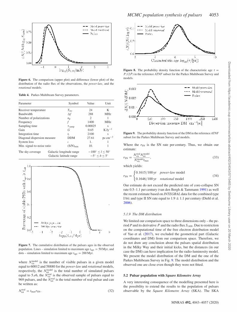
5.1.5 The fit of radio-luminosity laws

Although the fit in the 2D marginal distributions of the comparisonspace (second and third columns of Fig. 5) seems to be in generalagreement with the observations, the comparison of the radio-fluxdistribution (see Fig. 6) shows some discrepancies. Our modelsunderestimate the lower radio fluxes, and overestimate the brightestobjects. Both models behave in the same way pointing to a possiblesystematic error in the method, or model description. The couplingof the P − P − S in both the optimization (comparison space),period evolution and radio-luminosity law, may have degeneratedthe problem – leading to too few observational constraints withregard to the number of free parameters. We also note that theintroduction a phenomenological death area (see equation 14)might have altered the distribution of pulsars in the P − P plane(see Fig. 5). We excluded the parameter � from our currentanalysis due to the complexity reduction of the computations.We plan to include the analysis of the death area in our futurework.

5.1.6 The kicks distribution

We are aware that Hobbs et al. (2005) may be an imperfectdistribution of the SN kicks, as stated in Faucher-Giguere & Kaspi(2006) or more recently in Verbunt, Igoshev & Cator (2017).However, the spatial distribution (see Section 2.4.2) is beyond thescope of this work. Moreover, by employing the Parkes MultibeamSurvey, we focus only on the Galactic disc towards the centre of theGalaxy (see Table 4), thus limiting our study to a younger subsetof the whole Galactic population. Any possible discrepancies in thekicks model are neglected by this choice.

5.1.7 Pulsar ages

We found that, within our model, a fraction of less then 1 per centof pulsars is older then 50 Myr (see Fig. 7). Because those pulsarsdo not contribute in any significant way to the likelihood and as aresult to MCMC and parameter estimation (a smaller 200-chainstest yielded similar results to presented therein), we neglected thispart of population. We limited the maximum age of pulsars tobe tage � 50 Myr. We do not contradict the observed kinematicages distribution (Noutsos et al. 2013). Our study is focused onthe Galactic disc population (see Table 4) and we are unable toeffectively compare with older kinematic population. Moreover,by the inclusion of the magnetic field decay, we greatly speedup the pulsars evolution track on the P − P plane. This maylead to incorrect comparison between the evolution (simulation)age and the characteristic age distribution. By computing the

MNRAS 492, 4043–4057 (2020)

Dow

nloaded from https://academ

ic.oup.com/m

nras/article-abstract/492/3/4043/5715465 by Swinburne Library user on 20 M

arch 2020

4052 M. Cieslar, T. Bulik and S. Osłowski

Figure 5. Observations – the subset of the ATNF catalogue (first row), power-law model (second row), and rotational model in the 2D marginalizations of thecomparison space P − P − S. The colours indicate density levels for a given pair of dimensions i, j (e.g. i = P and j = P for the first column). The contourlines relate to the observations in each plot. The dots represent observations that lay in the region with extremely low density.

characteristic age

τ = P

2P, (30)

we show in Fig. 8 that the distribution of models resemble theobserved sample and that it is possible to produce pulsars withτ�50 Myr.

5.1.8 Estimated SN rate

To derive the SN rate from our models, we assume that the modelledand real populations have similar age (tmax = 50 Myr), and that theratio of the number of visible pulsars Nvis to the total number ofpulsars Ntot is constant:

N realvis

N realtot

= Nmodelvis

Nmodeltot

, (31)

MNRAS 492, 4043–4057 (2020)

Dow

nloaded from https://academ

ic.oup.com/m

nras/article-abstract/492/3/4043/5715465 by Swinburne Library user on 20 M

arch 2020

MCMC population synthesis of pulsars 4053

Figure 6. The comparison (upper plot) and difference (lower plot) of thedistribution of the radio flux of the observations, the power-law, and therotational models.

Table 4. Parkes Multibeam Survey parameters.

Parameter Symbol Value Unit

Receiver temperature Trec 24 KBandwidth �f 288 MHzNumber of polarizations np 2 1Frequency f 1400 MHzSampling time τ samp 0.00025 sGain G 0.65 K Jy−1

Integration time ti 2100 sDiagonal dispersion measure DDM 27.61 pc cm−3

System loss ι 1. 1Min. signal-to-noise ratio (S/N)min 10. 1

The sky coverage Galactic longitude range −100◦ ≤ l ≤ 50◦Galactic latitude range −5◦ ≤ b ≤ 5◦

Figure 7. The cumulative distribution of the pulsars ages in the observedpopulation. Lines – simulation limited to maximum age tage = 50 Myr, anddots – simulation limited to maximum age tage = 200 Myr.

where Nmodelvis is the number of visible pulsars in a given model

equal to 60012 and 58880 for the power-law and rotational models,respectively, the Nmodel

tot is the total number of simulated pulsarsequal to 5.e6, the N real

vis is the observed sample of pulsars equal to969 pulsars, and the N real

tot is the total number of real pulsar and canbe written as:

N realtot = tmaxrSN. (32)

Figure 8. The probability density function of the characteristic age τ =P/(2P ) in the reference ATNF subset for the Parkes Multibeam Survey andmodels.

Figure 9. The probability density function of the DM in the reference ATNFsubset for the Parkes Multibeam Survey and models.

Where the rSN is the SN rate per century. Thus, we obtain ourestimate:

rSN = N realvis Nmodel

tot

Nmodelvis tmax

, (33)

which yields:

rSN ={

0.1615/100 yr power-law model

0.1646/100 yr rotational model(34)

Our estimate do not exceed the predicted rate of core-collapse SNrate 0.5–1.1 per century (van den Bergh & Tammann 1991) as wellthe recent estimate based on INTEGRAL data for the combined typeI b/c and type II SN rate equal to 1.9 ± 1.1 per century (Diehl et al.2006).

5.1.9 The DM distribution

We limited our comparison space to three dimensions only – the pe-riod P and its derivative P and the radio flux S1400. Due to restrictionon the computational time of the free electron distribution modelof Yao et al. (2017), we excluded the geometrical part (Galacticcoordinates and DM) from our comparison space. Therefore, wedo not draw any conclusion about the pulsars spatial distributionin the Milky Way and their initial kicks, but the distances (in ourcase the DM) can have implication for the radio-luminosity model.We present the model distribution of the DM and the one of theParkes Multibeam Survey in Fig. 9. The model distribution and theobserved one are close even though they were not fitted.

5.2 Pulsar population with Square Kilometre Array

A very interesting consequence of the modelling presented here isthe possibility to extend the results to the population of pulsarsobservable by the Square Kilometre Array (SKA). The SKA

MNRAS 492, 4043–4057 (2020)

Dow

nloaded from https://academ

ic.oup.com/m

nras/article-abstract/492/3/4043/5715465 by Swinburne Library user on 20 M

arch 2020

4054 M. Cieslar, T. Bulik and S. Osłowski

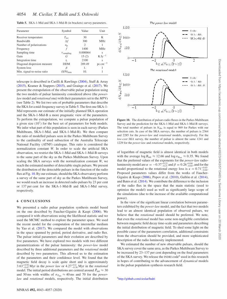
Table 5. SKA-1-Mid and SKA-1-Mid-B (in brackets) survey parameters.

Parameter Symbol Value Unit

Receiver temperature Trec 30 KBandwidth �f 300 MHzNumber of polarizations np 2 1Frequency f 1400 MHzSampling time τ sampling 0.000064 sGain G 15 (2) K Jy−1

Integration time ti 2100 sDiagonal dispersion measure DDM 289.49 pc cm−3

System loss β 1. 1Min. signal-to-noise ratio (S/N)min 10. 1

telescope is described in Carilli & Rawlings (2004), Staff & Array(2015), Kramer & Stappers (2015), and Grainge et al. (2017). Wepresent the extrapolation of the observable pulsar population usingthe two models of pulsar luminosity considered above (the power-law model and rotational one) with their parameters set to the MPVs(see Table 2). We list two sets of probable parameters that describethe SKA for a mid-frequency survey in Table 5. The first one SKA-1-Mid represents our estimate of the initially planned SKA operationand the SKA-1-Mid-B a more pragmatic view of the parameters.To perform the extrapolation, we compute a pulsar population ofa given size (107) for the best set of parameters for both models.We infer what part of this population is seen in each survey (ParkesMultibeam, SKA-1-Mid, and SKA-1-Mid-B). We then comparethe ratio of modelled pulsars seen in the Parkes Multibeam Surveyto the cardinality of used subsection of the Australia TelescopeNational Facility (ATNF) catalogue. This ratio is considered thenormalization constant W. In order to scale the artificial SKAobservation, we restrict the SKA-1-Mid and SKA-1-Mid-B surveysto the same part of the sky as the Parkes Multibeam Survey. Uponscaling the SKA surveys with the normalization constant W, wereach the estimated number of detectable single pulsars. We presentthe distribution of the detectable pulsars in the function of the radioflux at Fig. 10. By our estimate, should the SKA observatory performa survey of the same part of sky as the Parkes Mutlibeam Survey,we would reach an increase in detected radio pulsars by 23 per centor 137 per cent for the SKA-1-Mid-B and SKA-1-Mid survey,respectively.

6 C O N C L U S I O N S

We presented a radio pulsar population synthesis model basedon the one described by Faucher-Giguere & Kaspi (2006). Wecompared it with observations using the likelihood statistic and weused the MCMC method to explore the parameter space. We usedthe recent model for the computation of the interstellar mediumby Yao et al. (2017). We compared the model with observationsin the space spanned by period, period derivative, and radio flux.The pulsar initial parameters and their evolution are described byfive parameters. We have explored two models with two differentparametrizations of the pulsar luminosity: the power-law modeldescribed by three additional parameters and the rotational modeldescribed by two parameters. This allowed us to the estimationof the parameters and their confidence level. We found that themagnetic field decay is scale quite short and is approximately3.63+0.94

−0.47 Myr in the power law or 4.27+0.4−0.38 Myr in the rotational

model. The initial period distributions are centred around Pinit ≈ 30and 50 ms with widths of σPinit ≈ 40 ms and 70 for the power-law and rotational models, respectively. The initial distribution

Figure 10. The distribution of pulsars radio fluxes in the Parkes MultibeamSurvey and the prediction for the SKA-1-Mid and SKA-1-Mid-B surveys.The total number of pulsars in Nobs is equal to 969 for Parkes with ourselection cuts. In case of the SKA surveys, the number of pulsars is 2364and 2285 for the power-law and rotational models, respectively. For thelow-cost SKA survey, the number of pulsar is almost the same 1241 and1229 for the power-law and rotational models, respectively.

of logarithm of magnetic field is almost identical in both modelswith the average log Binit ≈ 12.66 and log σBinit ≈ 0.35. We foundthat the preferred values of the exponents for the power-law radio-luminosity model are α = −0.37+0.22

−0.21 and β = 0.26+0.04−0.02, and for the

model proportional to the rotational energy loss is κ = 0.71+0.03−0.04.

Proposed parameters values differ from the works of Faucher-Giguere & Kaspi (2006), Popov et al. (2010), Gullon et al. (2014),and Bates et al. (2014). We contribute the difference to the inclusionof the radio flux in the space that the main statistic (used tooptimize the model) used as well as significantly large scope ofthe simulations (due to the increase of the available computationalpower).

In the view of the significant linear correlation between parame-ters exhibited by the power-law model, and the fact that two modelslead to an almost identical population of observed pulsars, webelieve that the rotational model should be preferred. We note,that even the rotational model has some non-negligible correlationbetween magnetic field decay time-scale and parameters describingthe initial distribution of magnetic field. To shed some light on thepossible cause of the parameters correlation, additional constraintsfrom the observation should be provided, and more sophisticateddescription of the radio luminosity implemented.

We estimated the number of new observable pulsars, should theSKA survey cover the same area, as the Parkes Multibeam Survey tobe increased by 23–137 per cent depending on the final parametersof the SKA survey. We release the INDRI code6 used in this researchin hopes of contributing to the advancement of dynamical modelsin the pulsar population synthesis research field.

6http://github.com/cieslar/Indri

MNRAS 492, 4043–4057 (2020)

Dow

nloaded from https://academ

ic.oup.com/m

nras/article-abstract/492/3/4043/5715465 by Swinburne Library user on 20 M

arch 2020

MCMC population synthesis of pulsars 4055

AC K N OW L E D G E M E N T S

MC and TB were supported by the National Science Centre (NCN)grant no. UMO-2014/14/M/ST9/00707. MC acknowledges supportfrom Foundation for Polish Science (FNP) Master2013 Subsidyas well as from the NCN grant no. 2016/22/E/ST9/00037. TB isgrateful for support from TEAM/2016-3/19 from the FNP. SOacknowledges support from the Alexander von Humboldt Foun-dation and Australian Research Council grant Laureate FellowshipFL150100148.

In our work, we used the Mersenne Twister pseudo-randomnumber generator by Matsumoto & Nishimura (1998). We thankMichał Bejger and Paweł Ciecielag from Nicolaus CopernicusAstronomical Center (Polish Academy of Sciences, Warsaw) forhousing part of our simulations on the bigdog cluster located at theInstitute of Mathematics (Polish Academy of Sciences, Warsaw).The majority of the computations were performed on the OzSTARNational Facility at Swinburne University of Technology. OzSTARis funded by Swinburne University of Technology and the NationalCollaborative Research Infrastructure Strategy (NCRIS).

RE FERENCES

Arzoumanian Z., Chernoff D. F., Cordes J. M., 2002, ApJ, 568, 289Bates S. D., Lorimer D. R., Rane A., Swiggum J., 2014, MNRAS, 439,

2893Belczynski K., Benacquista M., Bulik T., 2010, ApJ, 725, 816Beskin V. S., Chernov S. V., Gwinn C. R., Tchekhovskoy A. A., 2015,

Space Sci. Rev., 191, 207Bhat N. D. R., Cordes J. M., Camilo F., Nice D. J., Lorimer D. R., 2004,

ApJ, 605, 759Blondin J. M., Mezzacappa A., 2007, Nature, 445, 58Carilli C. L., Rawlings S., 2004, New Astron. Rev., 48, 979Cordes J. M., Lazio T. J. W., 2002, preprint (arXiv: 0207156)Cordes J. M., Lazio T. J. W., 2003, preprint (arXiv: 0301598)Dewey R. J., Taylor J. H., Weisberg J. M., Stokes G. H., 1985, ApJ, 294,

L25Diehl R. et al., 2006, Nature, 439, 45Faucher-Giguere C.-A., Kaspi V. M., 2006, ApJ, 643, 332Foreman-Mackey D., Hogg D. W., Lang D., Goodman J., 2013, PASP, 125,

306Gilks W. R., Best N., Tan K., 1995, J. R. Stat. Soc. Ser. C, 44, 455Gold T., 1968, Nature, 218, 731Gonthier P. L., Story S. A., Clow B. D., Harding A. K., 2007, Ap&SS, 309,

245Goodman J., Weare J., 2010, Commun. Appl. Math. Comput. Sci., 5, 65Grainge K. et al., 2017, Astron. Rep., 61, 288Gullon M., Miralles J. A., Vigano D., Pons J. A., 2014, MNRAS, 443, 1891Hastings W. K., 1970, Biometrika, 57, 97Hewish A., Bell S. J., Pilkington J. D. H., Scott P. F., Collins R. A., 1969,

Nature, 224, 472Hobbs G., Lorimer D. R., Lyne A. G., Kramer M., 2005, MNRAS, 360, 974Igoshev A. P., Popov S. B., 2015, Astron. Nachr., 336, 831Kiel P. D., Hurley J. R., 2009, MNRAS, 395, 2326Kiel P. D., Hurley J. R., Bailes M., Murray J. R., 2008, MNRAS, 388, 393Kramer M., Stappers B., 2015, in Pulsar Science with the SKA, Advancing

Astrophysics with the Square Kilometre Array (AASKA14). Proceed-ings of Science, Trieste, Italy, p. 36

Levin L. et al., 2013, MNRAS, 434, 1387Lorimer D. R., 2011, in Torres D. F., Rea N., eds, High-Energy Emission

from Pulsars and their Systems. Springer Berlin Heidelberg, Berlin,Heidelberg, p. 21

MacKay D., 2003, Information Theory, Inference and Learning Algorithms.Cambridge Univ. Press, Cambridge

Manchester R. N. et al., 2001, MNRAS, 328, 17Manchester R. N., Hobbs G. B., Teoh A., Hobbs M., 2005, AJ, 129, 1993

Maron O., Kijak J., Kramer M., Wielebinski R., 2000, A&AS, 147,195

Marsaglia G., 1972, Ann. Math. Statist., 43, 645Matsumoto M., Nishimura T., 1998, ACM Trans. Model. Comput. Simul.,

8, 3Miyamoto M., Nagai R., 1975, PASJ, 27, 533Mosegaard K., Tarantola A., 1995, J. Geophys. Res., 100, 12Narayan R., Ostriker J. P., 1990, ApJ, 352, 222Noutsos A., Schnitzeler D. H. F. M., Keane E. F., Kramer M., Johnston S.,

2013, MNRAS, 430, 2281Osłowski S., Bulik T., Gondek-Rosinska D., Belczynski K., 2011, MNRAS,

413, 461Ostriker J. P., Gunn J. E., 1969, ApJ, 157, 1395Pacini F., 1967, Nature, 216, 567Paczynski B., 1990, ApJ, 348, 485Popov S. B., Prokhorov M. E., 2007, Phys. Usp., 50, 1123Popov S. B., Pons J. A., Miralles J. A., Boldin P. A., Posselt B., 2010,

MNRAS, 401, 2675Rantsiou E., Burrows A., Nordhaus J., Almgren A., 2011, ApJ, 732, 57Rudak B., Ritter H., 1994, MNRAS, 267, 513Scott D. W., 2015, Multivariate density estimation: theory, practice, and

visualization, John Wiley & Sons, New YorkShapiro S. L., Teukolsky S. A., 1986, Black Holes, White Dwarfs and

Neutron Stars: The Physics of Compact Objects. Cornell University,Ithaca, NY

Sharma S., 2017, ARA&A, 55, 213Braun R., Bourke T., Green J. A., Kaene E., Wagg J., 2015, in Advancing

Astrophysics with the Square Kilometer Array. Advancing Astrophysicswith the Square Kilometre Array (AASKA14), Proceedings of Science,Trieste, Italy

Tarantola A., 2005, Inverse Problem Theory and Methods for ModelParameter Estimation, Society for Industrial and Applied Mathematics,Philadelphia, US

Tauris T. M., Manchester R. N., 1998, MNRAS, 298, 625van den Bergh S., Tammann G. A., 1991, ARA&A, 29, 363Verbunt F., Igoshev A., Cator E., 2017, A&A, 608, A57Verlet L., 1967, Phys. Rev., 159, 98Wainscoat R. J., Cohen M., Volk K., Walker H. J., Schwartz D. E., 1992,

ApJS, 83, 111Yao J. M., Manchester R. N., Wang N., 2017, ApJ, 835, 29Yusifov I., Kucuk I., 2004, A&A, 422, 545Zhang C. M., Kojima Y., 2006, MNRAS, 366, 137

APPENDI X A :

In this appendix, for the completion purpose, we present the partsof the model that are identical to the model developed by Faucher-Giguere & Kaspi (2006).

A1 The Milky Way

A1.1 The Galactic potential

We use the well-established three-component Galactic potentialconsisting of the disc, the bulge, and the halo. The bulge �Bulge andthe disc �Disc gravitational potentials are adopted after Miyamoto &Nagai (1975). The formula describing the bulge is:

�Bulge = − GMb√b2

b + r2(A1)

where Mb = 1.12 × 1010 M�, bb = 0.277 kpc, and r = (x2 + y2 +z2)1/2. We model the disc potential as:

�Disc = − GMd√(ad +

√b2

d + z2)2 + ρ2

(A2)

MNRAS 492, 4043–4057 (2020)

Dow

nloaded from https://academ

ic.oup.com/m

nras/article-abstract/492/3/4043/5715465 by Swinburne Library user on 20 M

arch 2020

4056 M. Cieslar, T. Bulik and S. Osłowski

Table A1. Spiral arms parameters.

Arm k rad ρ0 kpc θ0 rad

Norma 4.25 3.48 1.57Carina-Sagittarius 4.25 3.48 4.71Perseus 4.89 4.90 4.05Crux-Scutum 4.89 4.90 0.95

where Md = 8.78 × 1010 M�, ad = 4.2 kpc, and bd = 0.198 kpc,and ρ = (x2 + y2)1/2. We use the halo potential �Halo following themodel of Paczynski (1990):

�Halo = −GMh

2rc

(2rc

rarctan

(r

rc

)+ log

(r2

r2c

+ 1

))(A3)

where Mh = 5 × 1010 M� and rc = 6 kpc. As the associated densityof the halo is diverging so we cut the halo potential at rcut = 100 kpc,see e.g. Belczynski, Benacquista & Bulik (2010). We neglect thedependence of the Galactic potential on the individual Galacticarms.

A1.2 The initial positions of pulsars

We adopt the initial position distribution after Faucher-Giguere &Kaspi (2006) with the assumption that pulsars are born inside theGalactic spiral arms. Following them, we exclude the Local Arm asthe origin of the pulsars. The centroids of each arm are describedas logarithmic spirals (Wainscoat et al. 1992):

θ (ρ) = k log

(ρ

ρ0

)+ θ0 (A4)

with their parameters listed in Table A1. With equal probabilitywe chose the arm in which pulsar is born. The distance ρraw fromthe centre of the Galaxy is drawn using the stellar surface densitydistribution in the Galactic plane (Yusifov & Kucuk 2004):

ξ (ρraw) ∼(

ρraw + R1

R� + R1

)a

exp

(−b

(ρraw − R�R� + R1

))(A5)

where a = 1.64, b = 4.01, R1 = 0.55 kpc, and R� = 8.5 kpc is thedistance of the Sun from the Galactic centre. We insert the radialdistance into equation (A4) to obtain the position along the spiralarm’s centroid (ρraw, θ raw). This position is then smeared by addinga correction to the angle θ raw to avoid artificial structures in theGalactic centre:

θwide = θraw + θcorr exp−0.35ρraw

kpc(A6)

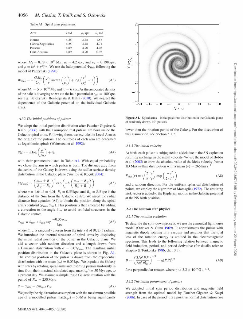
where θ corr is randomly chosen from the interval of [0, 2π ) radians.We introduce the internal structure of spiral arms by displacingthe initial radial position of the pulsar in the Galactic plane. Weadd a vector with random direction and a length drawn froma Gaussian distribution with σ = 0.07ρraw. The resulting initialposition distribution in the Galactic plane is shown in Fig. A1.The vertical position of the pulsar is drawn from the exponentialdistribution with the mean 〈z0〉 = 0.05 kpc. We populate the Galaxywith stars by rotating spiral arms and inserting pulsars uniformly intime from their maximal simulated age, max(tage) = 50 Myr ago, toa present day. We assume a simple, rigid Galactic rotation with theperiod of Prot = 250 Myr:

θ = θwide − 2πtage/Prot (A7)

We justify the rigid rotation assumption with the maximum possibleage of a modelled pulsar max(tage) = 50 Myr being significantly

Figure A1. Spiral arms – initial positions distribution in the Galactic planeof randomly drawn, 107 pulsars.

lower then the rotation period of the Galaxy. For the discussion ofthis assumption, see Section 5.1.7.

A1.3 The initial velocity

At birth, each pulsar is subjugated to a kick due to the SN explosionresulting in change in the initial velocity. We use the model of Hobbset al. (2005) to draw the absolute value of the kicks velocity from a1D Maxwellian distribution with a mean 〈v〉 = 265 km s−1:

Pkick(v) =√

2

π

v2

〈v〉3 exp

( −v2

2 〈v〉2

)(A8)

and a random direction. For the uniform spherical distribution ofpoints, we employ the algorithm of Marsaglia (1972). The resultingkick vector is added to the Keplerian motion in the Galactic potentialat the NS birth position.

A2 The neutron star physics

A2.1 The rotation evolution

To describe the spin-down process, we use the canonical lighthousemodel (Ostriker & Gunn 1969). It approximates the pulsar withmagnetic dipole rotating in a vacuum and assumes that the totalloss of the rotation energy is emitted in the electromagneticspectrum. This leads to the following relation between magneticfield induction, period, and period derivative (for details refer toShapiro & Teukolsky 1986, ch. 10.5):

B =(

3Ic3P P

8π2R6NS

)1/2

= η(P P )1/2 (A9)

for a perpendicular rotator, where η � 3.2 × 1019 G s−1/2.

A2.2 The initial parameters of pulsars

We adopted initial spin period distribution and magnetic fieldstrength from the optimal model by Faucher-Giguere & Kaspi(2006). In case of the period it is a positive normal distribution (we

MNRAS 492, 4043–4057 (2020)

Dow

nloaded from https://academ

ic.oup.com/m

nras/article-abstract/492/3/4043/5715465 by Swinburne Library user on 20 M

arch 2020

MCMC population synthesis of pulsars 4057

redraw negative values) centred at Pinit and with standard deviationσPinit . We initialize the magnetic field strength with values drawnfrom lognormal distribution centred at a value of log(Binit) and withstandard deviation log(σBinit ). All four variables presented aboveare used to parametrize the evolution model. We list their limits inTable 1.

A3 Radio properties

A3.1 The minimal detectable flux

We follow identical prescription as Osłowski et al. (2011) to modelradio selection effects. The minimal detectable flux of a pulsar isdescribed by the radiometer equation (Dewey et al. 1985) adjustedfor pulsating sources:

Smin = ι (S/N)min Tsys

G√

npti�f

√We

P − We(A10)

where the ι is a value describing system loss, Tsys is the systemtemperature, G is the gain, np represents the number of polarizations,

�f is the bandwidth, ti is the integration time, (S/N)min represents theminimal signal-to-noise ratio, We is the effective width of the pulse,and P is the pulsar spin period. We supply the formula with valuesappropriate to the Parkes Multibeam Survey (see Table 4). Forthe system temperature Tsys, we consider only the sky temperature

Tsky in the direction of the measurement and the receiver noisetemperatures Trec:

Tsys = Trec + Tsky (A11)

The effective width of the pulse We is a function of the intrinsicwidth Wi, the sampling time τ samp, the pulsar DM, the diagonaldispersion measure DDM (characteristic to the survey) and theinterstellar scattering time τ scatt describing the pulse widening dueto the multipath propagation (dissipation of the signal by the freeelectron clouds in the Galaxy). The effective width We formula takesform of:

W 2e = W 2

i + τ 2samp +

(τsamp

DM

DDM

)2

+ τ 2scatt (A12)

We obtained the interstellar scattering time τ scatt using the modeldeveloped by Bhat et al. (2004) in which τ scatt is a function of theDM. The minimal flux Smin, the effective width We, the systemtemperature Tsys and τ scattering were calculated using the functionsfrom the PSREVOLVE7code developed at the Centre for Astrophysicsand Supercomputing, Swinburne University of Technology.

7http://astronomy.swin.edu.au/ fdonea/psrevolve.html

This paper has been typeset from a TEX/LATEX file prepared by the author.

MNRAS 492, 4043–4057 (2020)

Dow

nloaded from https://academ

ic.oup.com/m

nras/article-abstract/492/3/4043/5715465 by Swinburne Library user on 20 M

arch 2020