28
Markov chain Monte Carlo(MCMC) Jin Young Choi 1

Markov chain Monte Carlo(MCMC)
Jin Young Choi
1

Outline
Monte Carlo : Sample from a distribution to estimate the distribution
Markov Chain Monte Carlo (MCMC)
‒ Applied to Clustering, Unsupervised Learning, Bayesian Inference
Importance Sampling
Metropolis-Hastings Algorithm
Gibbs Sampling
Markov Blanket in Sampling for Bayesian Network
Example: Estimation of Gaussian Mixture Model
2
𝑝 𝑥 𝐷 =𝑧,𝜃𝑝 𝑥, 𝑧, 𝜃 𝐷 = ? , 𝑝 𝑧|𝑥, 𝜃 =? , 𝑝 𝜃|𝑥, 𝑧 =?

Markov chain Monte Carlo(MCMC)
Monte Carlo : Sample from a distribution
- to estimate the distribution for GMM estimation, Clustering
(Labeling, Unsupervised Learning)
- to compute max, mean
Markov Chain Monte Carlo : sampling using “local” information
- Generic “problem solving technique”
- decision/inference/optimization/learning problem
- generic, but not necessarily very efficient
3

Monte Carlo Integration
General problem: evaluating
𝔼𝑃 ℎ 𝑋 = ∫ ℎ 𝑥 𝑃 𝑥 𝑑𝑥can be difficult. (∫ ℎ 𝑥 𝑃 𝑥 𝑑𝑥 < ∞)
If we can draw samples 𝑥(𝑠)~𝑃 𝑥 , then we can estimate
𝔼𝑃 ℎ 𝑋 ≈ തℎ𝑁 =1
𝑁
𝑠=1
𝑁
ℎ 𝑥 𝑠 .
Monte Carlo integration is great if you can sample from the target distribution
• But what if you can’t sample from the target?
• Importance sampling: Use of a simple distribution
4

Importance Sampling
Idea of importance sampling:
Draw the sample from a proposal distribution 𝑄(⋅) and re-weight the integral using importance weights so that the correct distribution is targeted
𝔼𝑃 ℎ 𝑋 = ∫ℎ 𝑥 𝑃 𝑥
𝑄 𝑥𝑄 𝑥 𝑑𝑥 = 𝔼𝑄
ℎ 𝑋 𝑃 𝑋
𝑄 𝑋.
Hence, given an iid sample 𝑥 𝑠 from 𝑄, our estimator becomes
𝐸𝑄ℎ 𝑋 𝑃 𝑋
𝑄 𝑋=1
𝑁
𝑠=1
𝑁ℎ 𝑥 𝑠 𝑃 𝑥 𝑠
𝑄 𝑥 𝑠
5

Limitations of Monte Carlo
Direct (unconditional) sampling
• Hard to get rare events in high-dimensional spaces Gibbs sampling
Importance sampling
• Do not work well if the proposal 𝑄 𝑥 is very different from target 𝑃 𝑥
• Yet constructing a 𝑄 𝑥 similar to 𝑃 𝑥 can be difficult Markov Chain
Intuition: instead of a fixed proposal 𝑄 𝑥 , what if we could use an adaptiveproposal?
• 𝑋𝑡+1 depends only on 𝑋𝑡, not on 𝑋0, 𝑋1, … , 𝑋𝑡−1• Markov Chain
6
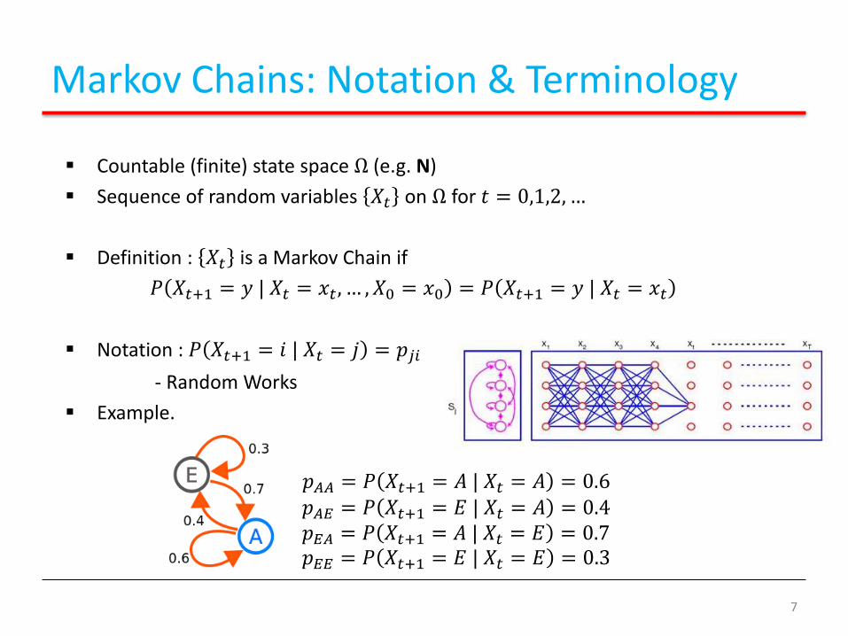
Markov Chains: Notation & Terminology
Countable (finite) state space Ω (e.g. N)
Sequence of random variables 𝑋𝑡 on Ω for 𝑡 = 0,1,2, …
Definition : 𝑋𝑡 is a Markov Chain if
𝑃 𝑋𝑡+1 = 𝑦 | 𝑋𝑡 = 𝑥𝑡, … , 𝑋0 = 𝑥0 = 𝑃 𝑋𝑡+1 = 𝑦 | 𝑋𝑡 = 𝑥𝑡
Notation : 𝑃 𝑋𝑡+1 = 𝑖 | 𝑋𝑡 = 𝑗 = 𝑝𝑗𝑖
- Random Works
Example.
𝑝𝐴𝐴 = 𝑃 𝑋𝑡+1 = 𝐴 | 𝑋𝑡 = 𝐴 = 0.6𝑝𝐴𝐸 = 𝑃 𝑋𝑡+1 = 𝐸 | 𝑋𝑡 = 𝐴 = 0.4𝑝𝐸𝐴 = 𝑃 𝑋𝑡+1 = 𝐴 | 𝑋𝑡 = 𝐸 = 0.7𝑝𝐸𝐸 = 𝑃 𝑋𝑡+1 = 𝐸 | 𝑋𝑡 = 𝐸 = 0.3
7

Markov Chains: Notation & Terminology
Let 𝑷 = 𝑝𝑖𝑗 - transition probability matrix
- dimension Ω × Ω
Let 𝜋𝑡 𝑗 = 𝑃 𝑋𝑡 = 𝑗
- 𝜋0 : initial probability distribution
Then 𝜋𝑡 𝑗 = σ𝑖 𝜋𝑡−1 𝑖 𝑝𝑖𝑗 = 𝜋𝑡−1𝑷 𝑗 = 𝜋0𝑷𝑡 𝑗
𝜋𝑡 = 𝜋𝑡−1𝑷 = 𝜋𝑡−2𝑷2 =∙∙∙= 𝜋0𝑷
𝑡
8

Markov Chains: Fundamental Properties
Theorem:
- If the limit lim𝑡→∞
𝑃𝑡 = 𝑃 exists and Ω is finite, then
𝜋𝑃 𝑗 = 𝜋 𝑗 and σ𝑗 𝜋 𝑗 = 1
and such 𝜋 is an unique solution to 𝜋𝑷 = 𝜋 (𝜋 is called a stationary distribution)
- No matter where we start, after some time, we will be in any state 𝑗 with probability ~ 𝜋 𝑗
9
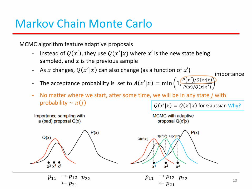
Markov Chain Monte Carlo
MCMC algorithm feature adaptive proposals
- Instead of 𝑄 𝑥′ , they use 𝑄(𝑥′|𝑥) where 𝑥′ is the new state being sampled, and 𝑥 is the previous sample
- As 𝑥 changes, 𝑄 𝑥′|𝑥 can also change (as a function of 𝑥′)
- The acceptance probability is set to 𝐴 𝑥′|𝑥 = min 1,𝑃 𝑥′ /𝑄 𝑥′|𝑥
𝑃 𝑥 /𝑄 𝑥|𝑥′
- No matter where we start, after some time, we will be in any state 𝑗 with probability ~ 𝜋 𝑗
10→ 𝑝12← 𝑝21
𝑝22𝑝11 → 𝑝12← 𝑝21
𝑝22𝑝11
importance
𝑄 𝑥′|𝑥 = 𝑄 𝑥′|𝑥 for Gaussian Why?

Metropolis-Hastings
Draws a sample 𝑥′ from 𝑄 𝑥′|𝑥 , where 𝑥 is the previous sample
The new sample 𝑥′ is accepted or rejected with some probability 𝐴 𝑥′|𝑥
• This acceptance probability is 𝐴 𝑥′|𝑥 = min 1,𝑃 𝑥′ /𝑄 𝑥′|𝑥
𝑃 𝑥 /𝑄 𝑥|𝑥′
• 𝐴 𝑥′|𝑥 is like a ratio of importance sampling weights
•𝑃 𝑥′
𝑄 𝑥′ 𝑥is the importance weight for 𝑥′,
𝑃 𝑥
𝑄 𝑥|𝑥′is the importance weight for 𝑥
• We divide the importance weight for 𝑥′ by that of 𝑥
• Notice that we only need to compute 𝑃 𝑥′ /𝑃 𝑥 rather than 𝑃 𝑥′ or 𝑃 𝑥 separately
• 𝐴 𝑥′ 𝑥 ensures that, after sufficiently many draws, our samples will come from the true distribution 𝑃(𝑥)
11
𝔼𝑃 ℎ 𝑋 = ∫ℎ 𝑥 𝑃 𝑥
𝑄 𝑥𝑄 𝑥 𝑑𝑥 = 𝔼𝑄
ℎ 𝑋 𝑃 𝑋
𝑄 𝑋
𝑄 𝑥′|𝑥 = 𝑄 𝑥′|𝑥 for Gaussian Why?

The MH Algorithm
Initialize starting state 𝑥(0),
Burn-in: while samples have “not converged”
• 𝑥 = 𝑥(𝑡)
• 𝑡 = 𝑡 + 1
• Sample 𝑥∗~𝑄(𝑥∗|𝑥) // draw from proposal
• Sample 𝑢~Uniform 0,1 // draw acceptance threshold
• If 𝑢 < 𝐴 𝑥∗ 𝑥 = min 1,𝑃 𝑥∗ 𝑄(𝑥|𝑥∗)
𝑃 𝑥 𝑄 𝑥∗|𝑥, 𝑥(𝑡)= 𝑥∗ // transition
• Else 𝑥(𝑡) = 𝑥 // stay in current state
• Repeat until converging
12
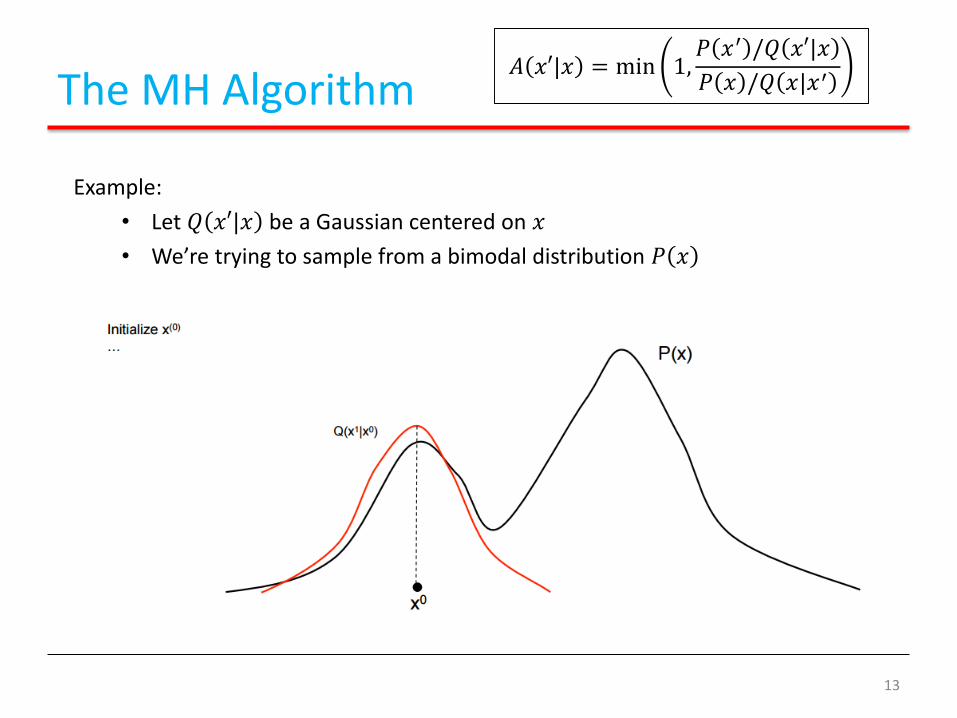
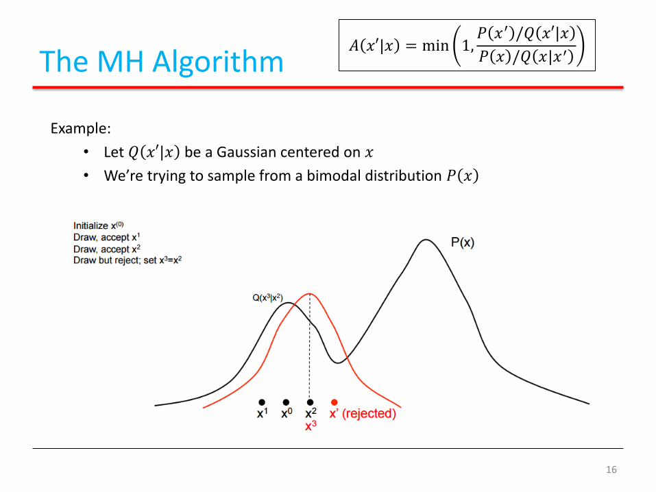
The MH Algorithm
Example:
• Let 𝑄 𝑥′|𝑥 be a Gaussian centered on 𝑥
• We’re trying to sample from a bimodal distribution 𝑃 𝑥
𝐴 𝑥′|𝑥 = min 1,𝑃 𝑥′ /𝑄 𝑥′|𝑥
𝑃 𝑥 /𝑄 𝑥|𝑥′
13

The MH Algorithm
Example:
• Let 𝑄 𝑥′|𝑥 be a Gaussian centered on 𝑥
• We’re trying to sample from a bimodal distribution 𝑃 𝑥
14
𝐴 𝑥′|𝑥 = min 1,𝑃 𝑥′ /𝑄 𝑥′|𝑥
𝑃 𝑥 /𝑄 𝑥|𝑥′
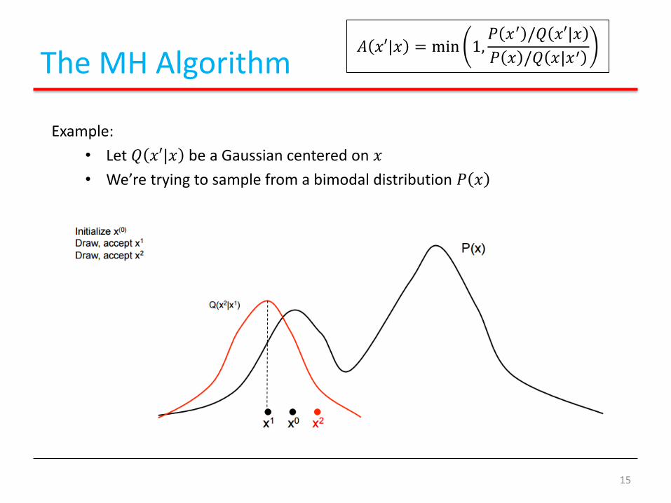
The MH Algorithm
Example:
• Let 𝑄 𝑥′|𝑥 be a Gaussian centered on 𝑥
• We’re trying to sample from a bimodal distribution 𝑃 𝑥
15
𝐴 𝑥′|𝑥 = min 1,𝑃 𝑥′ /𝑄 𝑥′|𝑥
𝑃 𝑥 /𝑄 𝑥|𝑥′
The MH Algorithm
Example:
• Let 𝑄 𝑥′|𝑥 be a Gaussian centered on 𝑥
• We’re trying to sample from a bimodal distribution 𝑃 𝑥
16
𝐴 𝑥′|𝑥 = min 1,𝑃 𝑥′ /𝑄 𝑥′|𝑥
𝑃 𝑥 /𝑄 𝑥|𝑥′

The MH Algorithm
Example:
• Let 𝑄 𝑥′|𝑥 be a Gaussian centered on 𝑥
• We’re trying to sample from a bimodal distribution 𝑃 𝑥
17
𝐴 𝑥′|𝑥 = min 1,𝑃 𝑥′ /𝑄 𝑥′|𝑥
𝑃 𝑥 /𝑄 𝑥|𝑥′

The MH Algorithm
Example:
• Let 𝑄 𝑥′|𝑥 be a Gaussian centered on 𝑥
• We’re trying to sample from a bimodal distribution 𝑃 𝑥
18
𝐴 𝑥′|𝑥 = min 1,𝑃 𝑥′ /𝑄 𝑥′|𝑥
𝑃 𝑥 /𝑄 𝑥|𝑥′

The MH Algorithm
Example:
• Let 𝑄 𝑥′|𝑥 be a Gaussian centered on 𝑥
• We’re trying to sample from a bimodal distribution 𝑃 𝑥
19
𝐴 𝑥′|𝑥 = min 1,𝑃 𝑥′ /𝑄 𝑥′|𝑥
𝑃 𝑥 /𝑄 𝑥|𝑥′

The MH Algorithm
Example:
• Let 𝑄 𝑥′|𝑥 be a Gaussian centered on 𝑥
• We’re trying to sample from a bimodal distribution 𝑃 𝑥
20
𝐴 𝑥′|𝑥 = min 1,𝑃 𝑥′ /𝑄 𝑥′|𝑥
𝑃 𝑥 /𝑄 𝑥|𝑥′
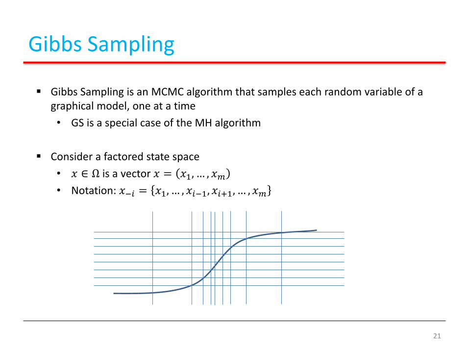
Gibbs Sampling
Gibbs Sampling is an MCMC algorithm that samples each random variable of a graphical model, one at a time
• GS is a special case of the MH algorithm
Consider a factored state space
• 𝑥 ∈ Ω is a vector 𝑥 = 𝑥1, … , 𝑥𝑚• Notation: 𝑥−𝑖 = 𝑥1, … , 𝑥𝑖−1, 𝑥𝑖+1, … , 𝑥𝑚
21

Gibbs Sampling
The GS algorithm:
1. Suppose the graphical model contains variables 𝑥1, … , 𝑥𝑛2. Initialize starting values for 𝑥1, … , 𝑥𝑛3. Do until convergence:
1. Pick a component 𝑖 ∈ 1, … , 𝑛
2. Sample value of 𝑧~𝑃 𝑥𝑖|𝑥−𝑖 , and update 𝑥𝑖 ← 𝑧
When we update 𝑥𝑖, we immediately use its new value for sampling other variables 𝑥𝑗
𝑃 𝑥𝑖|𝑥−𝑖 achieves the acceptance probability in MH algorithm.
22
𝐴 𝑥′|𝑥 = min 1,𝑃 𝑥′ /𝑄 𝑥′|𝑥
𝑃 𝑥 /𝑄 𝑥|𝑥′

Markov Blankets
The conditional 𝑃 𝑥𝑖 𝑥−𝑖 can be obtained using Markov Blanket
• Let 𝑀𝐵(𝑥𝑖) be the Markov Blanket of 𝑥𝑖, then
𝑃 𝑥𝑖 | 𝑥−𝑖 = 𝑃 𝑥𝑖|MB 𝑥𝑖
For a Bayesian Network, the Markov Blanket of 𝑥𝑖 is the set containing its parents, children, and co-parents
23

Gibbs Sampling: An Example
Consider the GMM
• The data 𝑥 (position) are extracted from two Gaussian distribution
• We do NOT know the class 𝑦 of each data, and information of the Gaussian distribution
• Initialize the class of each data at 𝑡 = 0 to randomly
24
Gaussian with mean 3,−3 , variance 3
Gaussian with mean 1,2 , variance 2

Gibbs Sampling: An Example
Sampling 𝑃 𝑦𝑖 𝑥−𝑖 , 𝑦−𝑖) at 𝑡 = 1, we compute:
𝑃 𝑦𝑖 = 0 |𝑥−𝑖 , 𝑦−𝑖 ∝ 𝒩 𝑥𝑖|𝜇𝑥−𝑖,0, 𝜎𝑥−𝑖,0𝑃 𝑦𝑖 = 1 | 𝑥−𝑖 , 𝑦−𝑖 ∝ 𝒩 𝑥𝑖|𝜇𝑥−𝑖,1, 𝜎𝑥−𝑖,1
where𝜇𝑥−𝑖,𝐾 = 𝑀𝐸𝐴𝑁 𝑋𝑖𝐾 , 𝜎𝑥−𝑖,𝐾 = 𝑉𝐴𝑅 𝑋𝑖𝐾𝑋𝑖𝐾 = 𝑥𝑗 | 𝑥𝑗 ∈ 𝑥−𝑖 , 𝑦𝑗 = 𝐾
And update 𝑦𝑖 with 𝑃 𝑦𝑖 |𝑥−𝑖 , 𝑦−𝑖 and repeat for all data
25
Iteration of 𝑖 at the same 𝑡
0 1
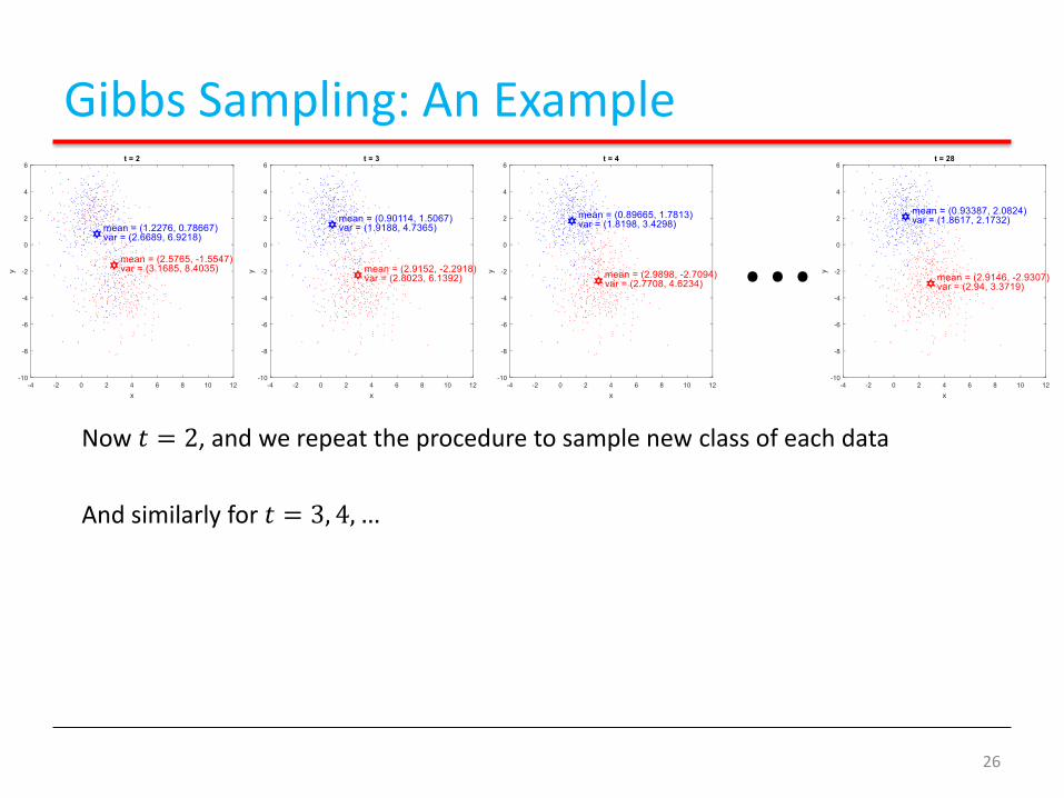
Gibbs Sampling: An Example
Now 𝑡 = 2, and we repeat the procedure to sample new class of each data
And similarly for 𝑡 = 3, 4, …
26
⋅⋅⋅

Gibbs Sampling: An Example
Data 𝑖’s class can be chosen with tendency of 𝑦𝑖• The classes of the data can be oscillated after the sufficient sequences
• We can assume the class of datum as more frequently selected class
In the simulation, the final class is correct with the probability of 94.9% at 𝑡 =100
27

Interim Summary
Markov Chain Monte Carlo methods use adaptive proposals 𝑄 𝑥′ 𝑥 to sample from the true distribution 𝑃 𝑥
Metropolis-Hastings allows you to specify any proposal 𝑄 𝑥′|𝑥
• But choosing a good 𝑄 𝑥′|𝑥 requires care
Gibbs sampling sets the proposal 𝑄 𝑥𝑖′|𝑥−1 to the conditional distribution 𝑃 𝑥𝑖
′|𝑥−1• Acceptance rate always 1.
• But remember that high acceptance usually entails slow exploration
• In fact, there are better MCMC algorithms for certain models
28


