Markov Chains and Mixing Times - · PDF filethe Ising model in Chapter 15 are due ......

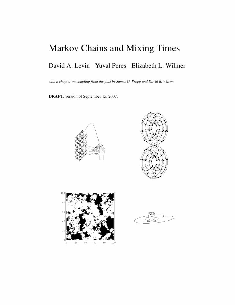
Markov Chains and Mixing Times

David A. Levin Yuval Peres Elizabeth L. Wilmer

with a chapter on coupling from the past by James G. Propp and David B. Wilson

DRAFT, version of September 15, 2007.

0 20 40 60 80 1000

20

40

60

80

100

1

David A. LevinDepartment of MathematicsUniversity of [email protected]

http://www.uoregon.edu/∼dlevin/

Yuval PeresMicrosoft Research

and University of California, [email protected]

http://stat-www.berkeley.edu/∼peres/

Elizabeth L. WilmerDepartment of MathematicsOberlin [email protected]

http://www.oberlin.edu/math/faculty/wilmer.html

http://www.uoregon.edu/~dlevin/

http://stat-www.berkeley.edu/~peres/

http://www.oberlin.edu/math/faculty/wilmer.html

2

Acknowledgements

The authors thank the Mathematical Sciences Research Institute, the NationalScience Foundation VIGRE grant to the Department of Statistics at the Universityof California, Berkeley, and National Science Foundation grants DMS-0244479and DMS-0104073 for support. We also thank Hugo Rossi for suggesting weembark on this project. Thanks to Jian Ding, Tom Hayes, Itamar Landau, YunLong, ¡¡¡¡¡¡¡ .mine Karola Meszaros, Shobhana Murali, and Sithparran =======Karola Meszarosfor, Shobhana Murali, Tomoyuki Shirai, and Sithparran ¿¿¿¿¿¿¿.r572 Vanniasegaram for corrections to an earlier version and making valuable sug-gestions. Yelena Shvets made the illustration in Section 7.5.1. The simulations ofthe Ising model in Chapter 15 are due to Raissa D’Souza. We thank Laszlo Lovaszfor useful discussions. We thank Robert Calhoun for technical assistance.

Contents

Chapter 1. Introduction 1

Chapter 2. Discrete Simulation 32.1. What Is Simulation? 32.2. About Random Numbers 42.3. Simulating Discrete Distributions and Sampling from Combinatorial

Sets 52.4. Randomly Ordered Decks Of Cards: Random Permutations 72.5. Random Colorings 82.6. Von Neumann unbiasing* 92.7. Problems 102.8. Notes 11

Chapter 3. Introduction to Finite Markov Chains 133.1. Finite Markov Chains 133.2. Simulating a Finite Markov Chain 163.3. Irreducibility and Aperiodicity 183.4. Random Walks on Graphs 193.5. Stationary Distributions 203.5.1. Definition 203.5.2. Hitting and first return times 213.5.3. Existence of a stationary distribution 213.5.4. Uniqueness of the stationary distribution 233.6. Reversibility and time reversals 233.7. Classifying the States of a Markov Chain* 243.8. Problems 243.9. Notes 28

Chapter 4. Some Interesting Markov Chains 294.1. Gambler’s Ruin 294.2. Coupon Collecting 304.3. Urn Models 314.3.1. The Bernoulli-Laplace model 314.3.2. The Ehrenfest urn model and the hypercube 324.3.3. The Polya urn model 334.4. Random Walks on Groups 334.4.1. Generating sets and irreducibility 35

3

4 CONTENTS

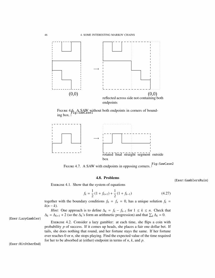
4.4.2. Parity of permutations and periodicity 354.4.3. Reversibility and random walks on groups 364.4.4. Transitive chains 364.5. Reflection Principles 364.5.1. The Ballot Theorem 404.6. Metropolis Chains and Glauber Dynamics 404.6.1. Metropolis chains 404.6.2. Glauber Dynamics 434.7. The Pivot Chain for Self-Avoiding Random Walk* 444.8. Problems 464.9. Notes 47

Chapter 5. Introduction to Markov Chain Mixing 495.1. Total Variation Distance 495.2. Coupling and Total Variation Distance 515.3. Convergence Theorem 545.4. Standardizing distance from stationarity 555.5. Mixing Time 575.6. Reversing Symmetric Chains 585.7. Ergodic Theorem* 595.8. Problems 605.9. Notes 61

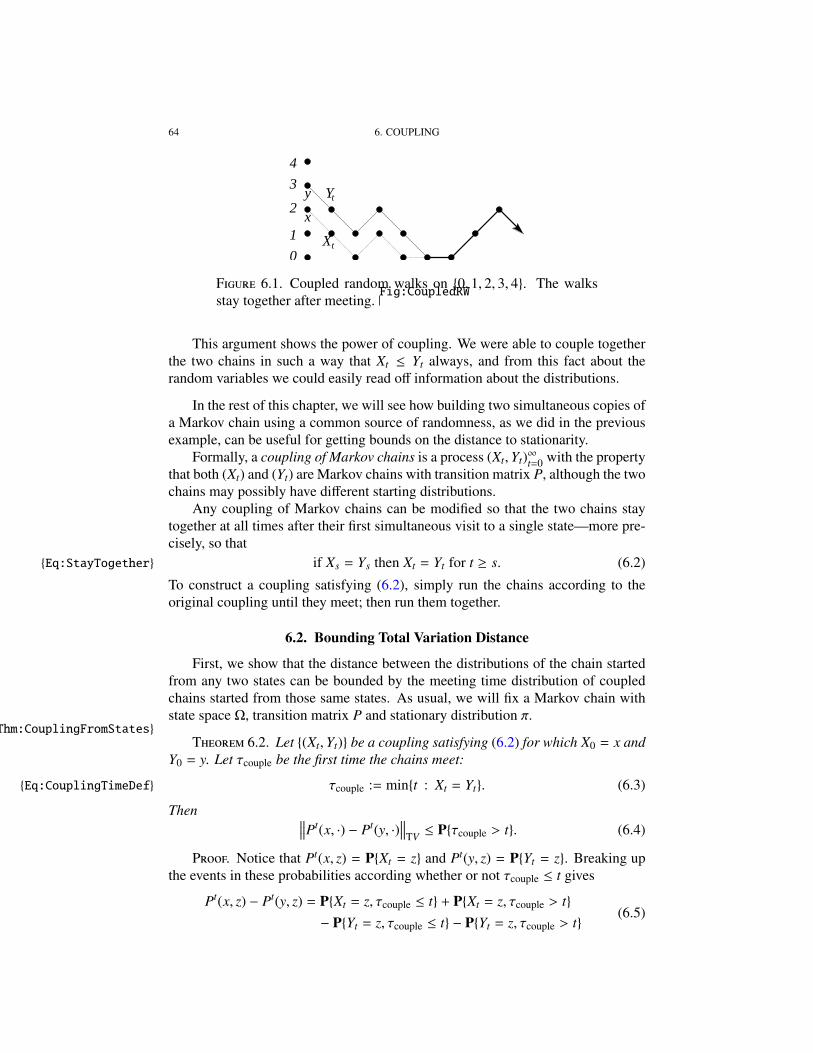
Chapter 6. Coupling 636.1. Definition 636.2. Bounding Total Variation Distance 646.3. Random Walk on the Torus 656.4. Random Walk on the Hypercube 676.5. Problems 686.6. Notes 68

Chapter 7. Strong Stationary Times 697.1. Two Examples 697.1.1. The top-to-random shuffle 697.1.2. Random walk on the hypercube 707.2. Stopping in the Stationary Distribution 707.2.1. Stopping times 707.2.2. Achieving equilibrium 717.3. Bounding Convergence using Strong Stationary Times 727.4. Examples 737.4.1. Two glued complete graphs 737.4.2. Random walk on the hypercube 737.4.3. Top-to-random shuffle 747.5. The Move-to-Front Chain 747.5.1. Move-to-front chain 747.6. Problems 74

CONTENTS 5

7.7. Notes 76

Chapter 8. Lower Bounds on Mixing Times and Cut-Off 778.1. Diameter Bound 778.2. Bottleneck Ratio 778.3. Distinguishing Statistics 828.3.1. Random walk on hypercube 848.4. Top-to-random shuffle 868.5. The Cut-Off Phenomenon 878.5.1. Random Walk on the Hypercube 898.5.2. Cut-off for the hypercube 898.6. East Model 938.7. Problems 948.8. Notes 95

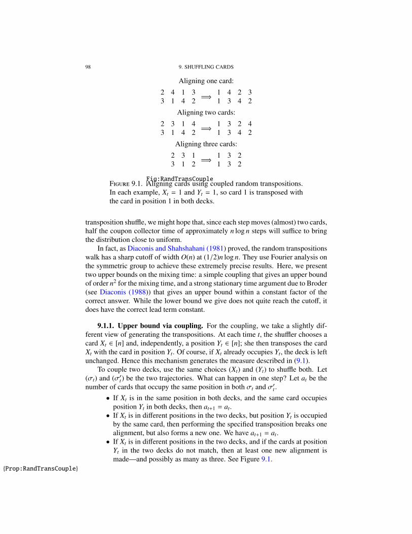
Chapter 9. Shuffling Cards 979.1. Random transpositions 979.1.1. Upper bound via coupling 989.1.2. Upper bound via strong stationary time 999.1.3. Lower bound 1019.2. Random adjacent transpositions 1029.2.1. Upper bound via coupling 1039.2.2. Lower bound for random adjacent transpositions 1049.3. Riffle shuffles 1059.4. Problems 1099.5. Notes 1109.5.1. Random transpositions 1109.5.2. Semi-random transpositions 1119.5.3. Riffle shuffles 112

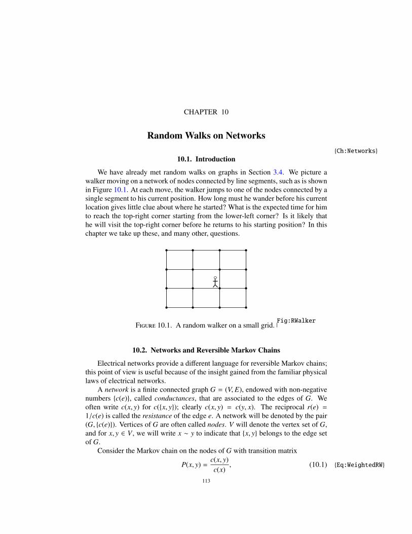
Chapter 10. Random Walks on Networks 11310.1. Introduction 11310.2. Networks and Reversible Markov Chains 11310.3. Harmonic Functions and Voltage 11410.4. Effective Resistance 11710.5. Escape Probabilities on a Square 12110.6. Problems 12210.7. Notes 123

Chapter 11. Hitting and Cover Times 12511.1. Hitting Times 12511.2. Hitting times and random target times 12611.3. Commute Time 12811.4. Hitting Times for the Torus 13011.5. Hitting Times for Birth-and-Death Chains 13211.6. Bounding Mixing Times via Hitting Times 133

6 CONTENTS

11.6.1. Cesaro mixing time 13711.7. Mixing for the Walker on Two Glued Graphs 13811.8. Cover Times 14011.9. The Matthews method 14111.10. Problems 145Notes 148

Chapter 12. Eigenvalues 14912.1. The Spectral Representation of a Transition Matrix 14912.2. Spectral Representation of Simple Random Walks 15112.2.1. The cycle 15112.2.2. Lumped chains and the path 15112.3. Product chains 15412.4. The Relaxation Time 15512.5. Bounds on Spectral Gap via Contractions 15712.6. An `2 Bound and Cut-Off for the Hypercube 15812.7. Wilson’s method and random adjacent transpositions 15912.8. Time Averages 16312.9. Problems 16512.10. Notes 166

Chapter 13. The Variational Principle and Comparison of Chains 16713.1. The Dirichlet Form 16713.2. The Bottleneck Ratio Revisited 16813.3. Proof of Lower Bound in Theorem 13.3* 16913.4. Comparison of Markov Chains 17013.4.1. The Comparison Theorem 17113.4.2. Random adjacent transpositions 17213.5. Expander Graphs* 17313.6. Problems 17413.7. Notes 174

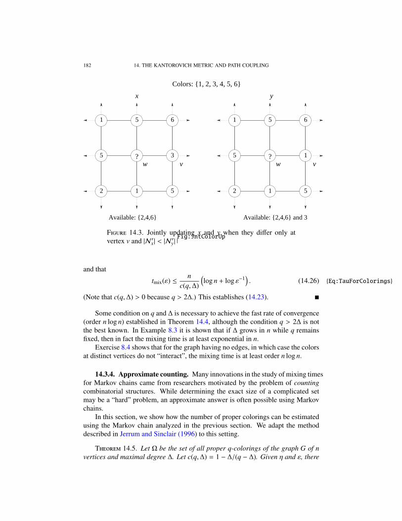
Chapter 14. The Kantorovich Metric and Path Coupling 17514.1. The Kantorovich Metric 17514.2. Path Coupling 17714.3. Application: Fast Mixing for Colorings 17914.3.1. Coloring a graph 17914.3.2. Coloring trees 17914.3.3. Mixing time for Glauber dynamics of random colorings 18014.3.4. Approximate counting 18214.4. Problems 18414.5. Notes 185

Chapter 15. The Ising Model 18715.1. Definitions 18715.1.1. Gibbs distribution 187

CONTENTS 7

15.1.2. Glauber dynamics 18815.2. Fast Mixing at High Temperature 18815.3. The Complete Graph 19015.4. Metastability 19115.5. Lower Bound for Ising on Square* 19115.6. Hardcore model 19315.7. The Cycle 19415.8. Notes 19515.8.1. A partial history 195

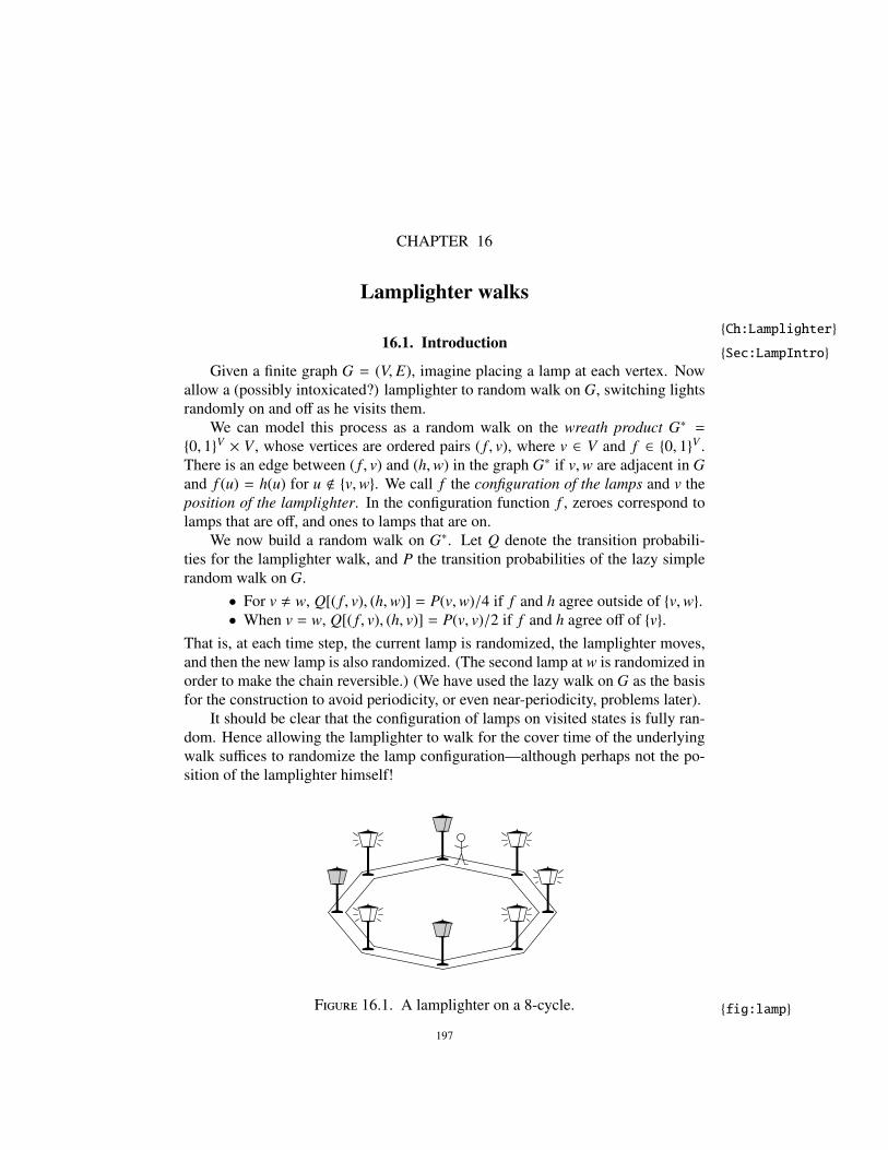
Chapter 16. Lamplighter walks 19716.1. Introduction 19716.2. A map of many parameters of Markov chains 19816.3. Relaxation time bounds 19816.4. Mixing time bounds 20016.5. Examples 20316.5.1. The complete graph 20316.5.2. Hypercube 20316.5.3. Tori 20316.6. Notes 204

Chapter 17. Continuous-time chains and simulation in the continuum* 20517.1. Continuous-Time Chains 20517.2. Continuous vs. discrete mixing 20717.3. Continuous Simulation 20917.3.1. Inverse distribution function method 20917.3.2. Acceptance-rejection sampling 20917.3.3. Simulating Normal random variables 21117.3.4. Sampling from the simplex 21317.4. Problems 21417.5. Notes 215

Chapter 18. Countable State-Space Chains* 21718.1. Recurrence and Transience 21718.2. Infinite Networks 21918.3. Positive Recurrence and Convergence 22118.4. Problems 225

Chapter 19. Martingales 22719.1. Definition and Examples 22719.2. Applications 23119.2.1. Gambler’s Ruin 23119.2.2. Waiting times for patterns in coin tossing 23119.3. Problems 232

Chapter 20. Coupling from the Past 23320.1. Introduction 233

8 CONTENTS

20.2. Monotone CFTP 23420.3. Perfect Sampling via Coupling from the past 23920.4. The hard-core model 24020.5. Random state of an unknown Markov chain 242

Appendix A. Notes on notation 245

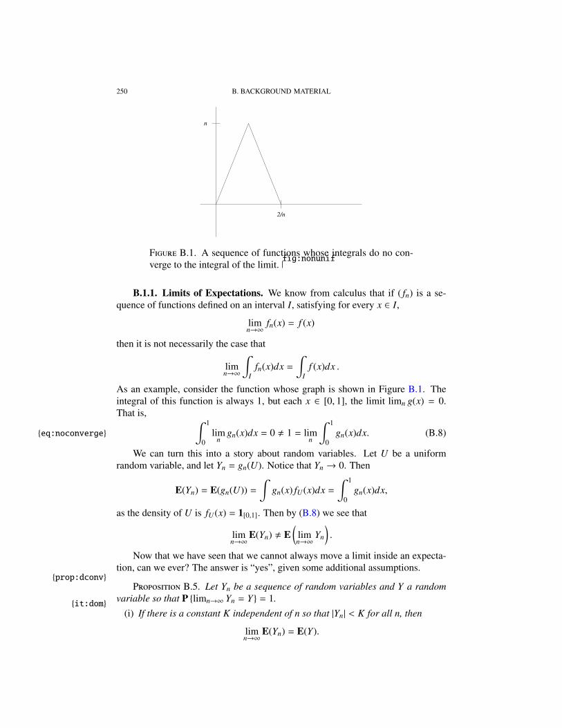
Appendix B. Background Material 247B.1. Probability Spaces and Random Variables 247B.1.1. Limits of Expectations 250B.2. Metric Spaces 251B.3. Linear Algebra 252B.4. Miscellaneous 252

Appendix C. Solutions to Selected Exercises 253

Appendix. Bibliography 277

CHAPTER 1

Introduction

Consider the following (inefficient) method of shuffling a stack of cards: a cardis taken from the top of the deck and placed at a randomly chosen location in thedeck. This is known as the top-to-random shuffle, not surprisingly.

We want a mathematical model for this type of process. Suppose that several ofthese shuffles have been performed in succession, each time changing the compo-sition of the deck a little bit. After the next shuffle, the cards will be in some order,and this ordering will depend only on the order of the cards now and the outcomeof the next shuffle. This property is important because to describe the evolutionof the deck, we need only specify the probability of moving from one ordering ofcards to any other ordering of cards in one shuffle.

The proper model for this card shuffling procedure is called a Markov chain.From any arrangements of cards, it is possible to get to any other by a sequenceof top-to-random shuffles. We may suspect that after many of these moves, thedeck should become randomly arranged. Indeed, this is the motivation for per-forming any kind of shuffle, as we are attempting to randomize the deck. Here, by“randomly arranged,” we mean that each arrangement of the cards is equally likely.

Under mild regularity conditions, a Markov chain converges to a unique sta-tionary distribution. Traditional undergraduate treatments of Markov chains ex-amine fixed chains as time goes to infinity. In the past two decades, a differentasymptotic analysis has emerged. For a Markov chain with a large state space, wecare about the finite number of steps needed to get the distribution reasonably closeto its limit. This number is known as the mixing time of the chain. There are nowmany methods for determining its behavior as a function of the geometry and sizeof the state space.

Aldous and Diaconis (1986) presented the concept of mixing times to a wideraudience, using card shuffling as a central example. Since then, both the field andits interactions with computer science and statistical physics have grown tremen-dously. Many of these exciting developments can and should be communicated toundergraduates. We hope to present this beautiful and relevant material in an acces-sible way. This book is intended for a second undergraduate course in probabilityand emphasizes current developments in the rigorous analysis of convergence timefor Markov chains.

The course will expose students to both key mathematical and probabilisticconcepts and the interactions of probability with other disciplines. The models weanalyze will largely be “particle systems” arising in statistical physics. Interest-ingly, many of these models exhibit phase transitions: the behavior of the model

1

2 1. INTRODUCTION

may change abruptly as a parameter describing local interactions passes througha critical value. For our particle systems, the mixing time may vary from “fast”(polynomial in the instance size n) to “slow” (exponential in n) as interaction pa-rameters pass through a critical value.

CHAPTER 2

Discrete Simulationch:simtechs

2.1. What Is Simulation?

Let X be a random unbiased bit:

PX = 0 = PX = 1 =12. (2.1)

If we assign the value 0 to the “heads” side of a coin, and the value 1 to the “tails”side, we can generate a bit which has the same distribution as X by tossing the coin.

Suppose now the bit is biased, so that

PX = 1 =14, PX = 0 =

34. (2.2) Eq:BiasedBit

Again using only our (fair) coin toss, we are able to easily generate a bit with thisdistribution: Toss the coin twice and assign the value 1 to the result “two heads”,and the value 0 to all other possible outcomes. Since the coin cannot rememberthe result of the first toss when it is tossed for the second time, the tosses areindependent and the probability of two heads is 1/4 (ideally, assuming the coinis perfectly symmetric.) This is a recipe for generating observations of a randomvariable which has the same distribution (2.2) as X. This is called a simulation ofX.

Consider the random variable Un which is uniform on the finite set0,

12n ,

22n , . . . ,

2n − 12n

. (2.3) Eq:Dyadics

This random variable is a discrete approximation to the uniform distribution on[0, 1]. If our only resource is the humble fair coin, we are still able to simulateUn: toss the coin n times to generate independent unbiased bits X1, X2, . . . , Xn, andoutput the value

n∑i=1

Xi

2i . (2.4) Eq:RandomSum

This random variables has the uniform distribution on the set in (2.3). (See Exercise2.9.)

Consequently, a sequence of independent and unbiased bits can be used to sim-ulate a random variable whose distribution is close to uniform on [0, 1]. A sufficientnumber of bits should be used to ensure that the error in the approximation is smallenough for any needed application. A computer can store a real number only tofinite precision, so if the value of the simulated variable is to be placed in computermemory, it will be rounded to some finite decimal approximation. With this in

3

4 2. DISCRETE SIMULATION

mind, the discrete variable in (2.4) will be just as useful as a variable uniform onthe interval of real numbers [0, 1].

2.2. About Random NumbersSec:PseudoRandom

Because most computer languages provide a built-in capability for simulatingrandom numbers chosen independently from the uniform density on the unit in-terval [0, 1], we will assume throughout this book that there is a ready source ofindependent uniform-[0, 1] random variables.

This assumption requires some further discussion, however. Since computersare finitary machines and can work with numbers of only finite precision, it is infact impossible for a computer to generate a continuous random variable. Not toworry: a discrete random variable which is uniform on, for example, the set in (2.3)is a very good approximation to the uniform distribution on [0, 1], at least when nis large.

A more serious issue is that computers do not produce truly random numbersat all. Instead, they use deterministic algorithms, called pseudorandom numbergenerators, to produce sequences of numbers that appear random. There are manytests which identify features which are unlikely to occur in a sequence of inde-pendent and identically distributed random variables. If a sequence produced by apseudorandom number generator can pass a battery of these tests, it is consideredan appropriate substitute for random numbers.

One technique for generating pseudorandom numbers is a linear congruentialsequence (LCS). Let x0 be an integer seed value. Given that xn−1 has been gener-ated, let

xn = (axn−1 + b) mod m. (2.5)

Here a, b and m are fixed constants. Clearly, this produces integers in 0, 1, . . . ,m;if a number in [0, 1] is desired, divide by m.

The properties of (x0, x1, x2, . . .) vary greatly depending on choices of a, b andm, and there is a great deal of art and science behind making judicious choices forthe parameters. For example, if a = 0, the sequence doesn’t look random at all!

Any linear congruential sequence is eventually periodic. (Exercise 2.8.) Theperiod of a LCS can be much less than m, the longest possible value.

The goal of any method for generating pseudorandom numbers is to generateoutput which is difficult to distinguish from truly random numbers using statisticalmethods. It is an interesting question whether a given pseudorandom number gen-erator is good. We will not enter into this issue here, but the reader should be awarethat the “random” numbers produced by today’s computers are not in fact random,and sometimes this can lead to inaccurate simulations. For an excellent discussionof these issues, see Knuth (1997).

2.3. SIMULATING DISCRETE DISTRIBUTIONS AND SAMPLING FROM COMBINATORIAL SETS 5

2.3. Simulating Discrete Distributions and Sampling from CombinatorialSets

A Poisson random variable X with mean λ has mass function

p(k) :=e−λλk

k!.

X can be simulated using a uniform random variable U as follows: subdivide theunit interval into adjacent subintervals I1, I2, . . . where the length of Ik is p(k).Because the chance a random point in [0, 1] falls in Ik is p(k), the index X forwhich U ∈ IX is a Poisson random variable with mean λ.

In principle, any discrete random variable can be simulated from a uniformrandom variable using this method. To be concrete, suppose X takes on the valuesa1, . . . , aN with probabilities p1, p2, . . . , pN . Let Fk :=

∑kj=1 p j (and F0 := 0), and

define φ : [0, 1]→ a1, . . . , aN by

φ(u) := ak if Fk−1 < u ≤ Fk. (2.6) Eq:DiscreteSim

If X = φ(U), where U is uniform on [0, 1], then PX = ak = pk. (Exercise 2.9.)Much of this book is concerned with the problem of simulating discrete distri-

butions. This may seem odd, as we just described an algorithm for simulating anydiscrete distribution!

One obstacle is that this recipe requires that the probabilities (p1, . . . , pN) areknown exactly, while in many applications these are only known up to constantmultiple. This is a more common situation than the reader may imagine, and infact many of the central examples treated in this book fall into this category.

A random element of a finite set is called a uniform sample if it is equally likelyto be any of the members of the set. Many applications require uniform samplesfrom combinatorial sets whose sizes are not known.

Example:SAW

E 2.1 (Self-avoiding walks). A self-avoiding walk in Z2 of length nis a sequence (z0, z1, . . . , zn) such that z0 = (0, 0), |zi − zi−1| = 1, and zi , z jfor i , j. See figure 2.1 for an example of length 6. Let Ξn be the collectionof all self-avoiding walks of length n. Chemical and physical structures such asmolecules and polymers are often modeled as “random” self-avoiding walks, thatis, as uniform samples from Ξn.

Unfortunately, a formula for the size of Ξn is not known. Although the size canbe calculated by computer for a fixed n if n is small enough, for sufficiently largen this is not possible. Nonetheless, we still desire (a practical) method for sam-pling uniformly from Ξn. We present a Markov chain in Example 4.23 whose statespace is the set of all self-avoiding walks of a given length and whose stationarydistribution is uniform.

A nearest-neighbor path 0 = v0, . . . , vn is non-reversing if vk , vk−2 for k =2, . . . , n. It is simple to generate a non-reversing path recursively. First choose v1uniformly at random from (0, 1), (1, 0), (0,−1), (−1, 0). Given that v0, . . . , vk−1 isa non-reversing path, choose vk uniformly from the three sites in Z2 at distance 1from vk−1 but different from vk−2.


F 2.1. A self-avoiding pathfig:SAW

Let Ξnrn be the set of non-reversing nearest-neighbor paths of length n. The

above procedure generates a uniform random sample from Ξnrn . (Exercise 2.10.)

Exercise 2.11 implies that if we try generating random non-reversing pathsuntil we get a self-avoiding path, the expected number of trials required growsexponentially in the length of the paths.

Many problems are defined for a family of structures indexed by instance size.For example, we desire an algorithm for generating uniform samples from self-avoiding paths of length n, for each n. The efficiency of solutions is measuredby the growth of run-time as a function of instance size. If the run-time growsexponentially in instance size, the algorithm is considered impractical.

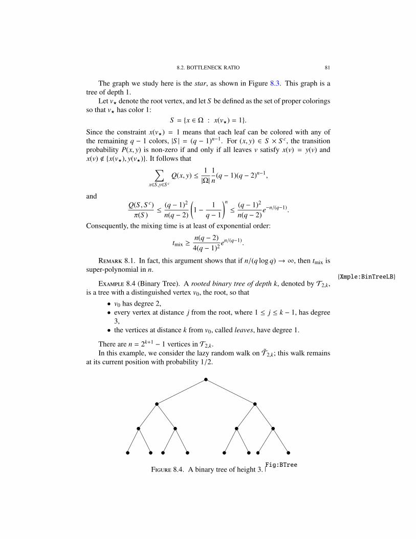
81 2 3 4 5 6 7

F 2.2. A configuration of the hard-core gas model with n =8. Colored circles correspond to occupied sites.

Xmple:1dHCE 2.2 (One dimensional hard-core gas). The hard-core gas models the

random distribution of particles under the restriction that the centers of any twoparticles are at least a fixed distance apart. In one dimension, the state space Ωn isfunctions ω : 1, 2, . . . , n → 0, 1 satisfying ω( j)ω( j+ 1) = 0 for j = 1, . . . , n− 1.We think of 1, 2, . . . , n as sites arranged linearly, and ω as describing a config-uration of particles on 1, . . . , n. The condition ω( j) = 1 indicates that site j isoccupied by a particle. The constraint ω( j)ω( j+1) = 0 means that no two adjacentsites are both occupied by particles.

Exercise 2.12 suggests an algorithm for inductively generating a random sam-ple from Ωn: Suppose you are able to generate random samples from Ωk fork ≤ n − 1. With probability fn−1/ fn+1, put a 1 at location n, a 0 at locationn − 1, and then generate a random element of Ωn−2 to fill out the configurationat 1, 2, . . . , n − 2. With the remaining probability fn/ fn+1, put a 0 at location nand fill out the positions 1, 2, . . . , n − 1 with a random element of Ωn−1.

Example:DominoTilingsE 2.3 (Domino Tilings). A domino tile is a 2×1 or 1×2 rectangle, and,

informally speaking, a domino tiling of a region is a partition of the region intodomino tiles, disjoint except along their boundaries.

Consider the set Tn,m of all domino tilings of an n × m checker board. Seefigure 2.3 for an element ofT6,6. Random domino tilings arise in statistical physics,

2.4. RANDOMLY ORDERED DECKS OF CARDS: RANDOM PERMUTATIONS 7

! ! ! ! ! ! ! ! ! !! ! ! ! ! ! ! ! ! !! ! ! ! ! ! ! ! ! !! ! ! ! ! ! ! ! ! !! ! ! ! ! ! ! ! ! !! ! ! ! ! ! ! ! ! !! ! ! ! ! ! ! ! ! !! ! ! ! ! ! ! ! ! !! ! ! ! ! ! ! ! ! !! ! ! ! ! ! ! ! ! !

" " " " " " " " " "" " " " " " " " " "" " " " " " " " " "" " " " " " " " " "" " " " " " " " " "" " " " " " " " " "" " " " " " " " " "" " " " " " " " " "" " " " " " " " " "" " " " " " " " " "

# # # # # # # # # ## # # # # # # # # ## # # # # # # # # ## # # # # # # # # ## # # # # # # # # ## # # # # # # # # ## # # # # # # # # ## # # # # # # # # ## # # # # # # # # ## # # # # # # # # #

F 2.3. A domino tiling of a 6 × 6 checkerboard.Fig:Domino

and it was a physicist who first completed the daunting combinatorial calculationof the size of Tn,m. (See Notes.)

Although the size N of Tn,m is known, the simulation method using (2.6) is notnecessarily the best. The elements of Tn,m must be enumerated so that when aninteger in 1, . . . ,N is selected, the corresponding tiling can be generated.

To summarize, we would like methods for picking at random from large combi-natorial sets which do not require enumerating the set or even knowing how manyelements are in the set. We will see later that Markov chain Monte Carlo oftenprovides such a method.

2.4. Randomly Ordered Decks Of Cards: Random PermutationsSec:SimPerms

If a game is to be played from a deck of cards, fairness usually requires that thedeck is completely random. That is, each of the 52! arrangements of the 52 cardsshould be equally likely.

An arrangements of cards in a particular order is an example of a permutation.Mathematically, a permutation on [n] := 1, 2, . . . , n is a mapping from [n] to itselfwhich is both one-to-one and onto. The collection Sn of all permutations on [n] iscalled the symmetric group.

We describe a simple algorithm for generating a random permutation. Let σ0be the identity permutation. For k = 1, 2, . . . , n − 1 inductively construct σk fromσk−1 by swapping the cards at location k and Jk, where Jk is an integer pickeduniformly in [k, n], independently of previous picks. More precisely,

σk(k) := σk−1(Jk), σk(Jk) := σk−1(k), and σk(i) := σk−1(i) for i , k, Jk.

The kth position refers to the image of k under the permutation. At the kthstage, a particular choice for the kth position has probability (n − k + 1)−1. Conse-quently, the probability of generating a particular permutation is

∏nk=1(n−k+1)−1 =

(n!)−1.


This method requires n steps, which is quite efficient. However, this is nothow any human being shuffles cards! For a standard deck of playing cards, itwould require 52 steps, many more operations than the usual handful of standardshuffles. We will discuss several methods of shuffling cards later, which generateapproximate random permutations on n things. Our interest will be in how manyshuffles need to be applied before the approximation to a random permutation isgood.

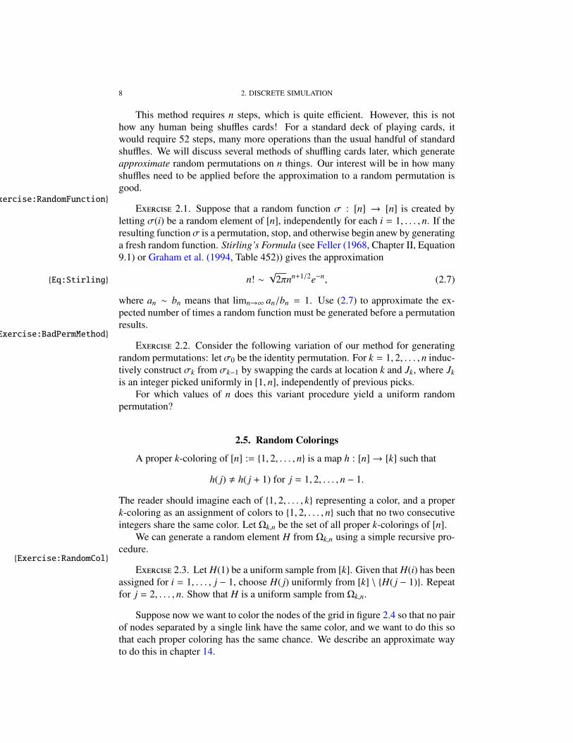
Exercise:RandomFunctionE 2.1. Suppose that a random function σ : [n] → [n] is created by

letting σ(i) be a random element of [n], independently for each i = 1, . . . , n. If theresulting functionσ is a permutation, stop, and otherwise begin anew by generatinga fresh random function. Stirling’s Formula (see Feller (1968, Chapter II, Equation9.1) or Graham et al. (1994, Table 452)) gives the approximation

n! ∼√

2πnn+1/2e−n, (2.7)Eq:Stirling

where an ∼ bn means that limn→∞ an/bn = 1. Use (2.7) to approximate the ex-pected number of times a random function must be generated before a permutationresults.

Exercise:BadPermMethod

E 2.2. Consider the following variation of our method for generatingrandom permutations: let σ0 be the identity permutation. For k = 1, 2, . . . , n induc-tively construct σk from σk−1 by swapping the cards at location k and Jk, where Jkis an integer picked uniformly in [1, n], independently of previous picks.

For which values of n does this variant procedure yield a uniform randompermutation?

2.5. Random Colorings

A proper k-coloring of [n] := 1, 2, . . . , n is a map h : [n]→ [k] such that

h( j) , h( j + 1) for j = 1, 2, . . . , n − 1.

The reader should imagine each of 1, 2, . . . , k representing a color, and a properk-coloring as an assignment of colors to 1, 2, . . . , n such that no two consecutiveintegers share the same color. Let Ωk,n be the set of all proper k-colorings of [n].

We can generate a random element H from Ωk,n using a simple recursive pro-cedure.

Exercise:RandomCol

E 2.3. Let H(1) be a uniform sample from [k]. Given that H(i) has beenassigned for i = 1, . . . , j − 1, choose H( j) uniformly from [k] \ H( j − 1). Repeatfor j = 2, . . . , n. Show that H is a uniform sample from Ωk,n.

Suppose now we want to color the nodes of the grid in figure 2.4 so that no pairof nodes separated by a single link have the same color, and we want to do this sothat each proper coloring has the same chance. We describe an approximate wayto do this in chapter 14.

2.6. VON NEUMANN UNBIASING* 9

F 2.4. How can we generate a proper coloring of the nodesuniformly at random?

Fig:PlaneGrid

2.6. Von Neumann unbiasing*

Suppose you have available an i.i.d. vector of biased bits, X1, X2, . . . , Xn. Thatis, each Xk is a 0, 1-valued random variable, with PXk = 1 = p , 1/2. Further-more, suppose that we do not know the value of p. Can we convert this randomvector into a (possibly shorter) random vector of independent and unbiased bits?

This problem was considered by Von Neumann (1951) in his work on earlycomputers. He described the following procedure: divide the original sequence ofbits into pairs, discard pairs having the same value, and for each discordant pair 01or 10, take the first bit. An example of this procedure is shown in figure 2.5; theextracted bits are shown in the second row.

original bits 00 11 01 01 10 00 10 10 11 10 01 · · ·

extracted unbiased · · 0 0 1 · 1 1 · 1 0 · · ·

discarded bits 0 1 · · · 0 · · 1 · · · · ·

XORed bits 0 0 1 1 1 0 1 1 0 1 1 · · ·

(2.8)

F 2.5. Extracting unbiased bits from biased bit stream.Fig:VN

Note that the number L of unbiased bits produced from (X1, . . . , Xn) is itself arandom variable. We denote by (Y1, . . . ,YL) the vector of extracted bits.

Exercise:VonNeumannE 2.4. Show that applying Von Neumann’s procedure to the vector

(X1, . . . , Xn) produces a vector (Y1, . . . ,YL) of random length L, which conditionedon L = m is uniformly distributed on 0, 1m.

How efficient is this method? For any algorithm for extracting random bits, letN be the number of fair bits generated using the first n of the original bits. Theefficiency is measured by the asymptotic rate

r(p) = lim supn→∞

E(N)n

. (2.9)

Let q := 1 − p.Exercise:VNEfficiency

E 2.5. Show that for the Von Neumann algorithm, E(N) = npq, and therate is r(p) = pq.


The Von Neumann algorithm throws out many of the original bits, which infact contain some unexploited randomness. By converting the discarded 00s and11s to 0s and 1s, we obtain a new vector Z = (Z1,Z2, . . . ,Zn/2−L) of bits. In theexample shown in figure 2.5, these bits are shown on the third line.

E 2.6. Prove: conditioned on L = m, the two vectors Y = (Y1, . . . ,YL)and Z = (Z1, . . . ,Zn/2−L) are independent, and the bits Z1, . . . ,Zn/2−L are indepen-dent.

The probability that Zi = 1 is p′ = p2/(p2 + q2). We can apply the algorithmagain on the independent bits Z. Given that L = m, Exercise 2.5 implies that theexpected number of fair bits we can extract from Z is

(length of Z)p′q′ =(n2− m

) ( p2

p2 + q2

) (q2

p2 + q2

). (2.10)

By Exercise 2.5 again, the expected value of L is npq. Hence the expected numberof extracted bits is

n[(1/2) − pq](

p2

p2 + q2

) (q2

p2 + q2

). (2.11)

Adding these bits to the original extracted bits yields a rate for the modified algo-rithm of

pq + [(1/2) − pq](

p2

p2 + q2

) (q2

p2 + q2

). (2.12)

A third source of bits is obtained by taking the XOR of adjacent pairs. (TheXOR of two bits a and b is 0 if and only if a = b.) Call this sequence U =

(U1, . . . ,Un/2). This is given on the fourth row in figure 2.5. It turns out that U isindependent of Y and Z, and applying the algorithm on U yields independent andunbiased bits. It should be noted, however, that given L = m, the bits in U are notindependent, as it contains exactly m 1’s.

Note that when the Von Neumann algorithm is applied to the sequence Z ofdiscarded bits and to U, it creates a new sequence of discarded bits. The algorithmcan be applied again to this sequence, improving the extraction rate.

Indeed, this can be continued indefinitely. This idea is developed in Peres(1992).

2.7. ProblemsExer:CoinSimUnif

E 2.7. Check that the random variable in (2.4) has the uniform distri-bution on the set in (2.3).

Exer:LCSPeriodicE 2.8. Show that if f : 1, . . . ,m → 1, . . . ,m is any function, and

xn = f (xn−1) for all n, then there is an integer k such that xn = xn+k eventually.That is, the sequence is eventually periodic.

Exer:UnifDiscDimE 2.9. Let U be uniform on [0, 1], and let X be the random variable

φ(U), where φ is defined as in (2.6). Show that X takes on the value ak withprobability pk.

2.8. NOTES 11

Exercise:NonRevE 2.10. A nearest-neighbor path 0 = v0, . . . , vn is non-reversing if vk ,

vk−2 for k = 2, . . . , n. It is simple to generate a non-reversing path recursively.First choose v1 uniformly at random from (0, 1), (1, 0), (0,−1), (−1, 0). Giventhat v0, . . . , vk−1 is a non-reversing path, choose vk uniformly from the three sitesin Z2 at distance 1 from vk−1 but different from vk−2.

Let Ξnrn be the set of non-reversing nearest-neighbor paths of length n. Show

that the above procedure generates a uniform random sample from Ξnrn .

Exer:SAWE 2.11. One way to generate a random self-avoiding path is to generate

non-reversing paths until a self-avoiding path is obtained.(a) Let cn,4 be the number of paths in Z2 which do not contain loops of length 4

at indices i ≡ 0 mod 4. More exactly, these are paths (0, 0) = v0, v1, . . . , vn sothat v4i , v4(i−1) for i = 1, . . . , n/4. Show that

cn,4 ≤[4(33) − 8

] [34 − 6

]dn/4e−1(2.13) Eq:NoLoops

(b) Conclude that the probability that a random non-reversing path of length n isself-avoiding is bounded above by e−αn for some fixed α > 0.

Exer:HCE 2.12. Recall that the Fibonacci numbers are defined by f0 := f1 := 1,

and fn := fn−1 + fn−2 for n ≥ 1. Show that the number of configurations in theone-dimensional hard-core model with n sites is fn+1.

Exer:HC2E 2.13. Show that the algorithm described in Example 2.2 generates a

uniform sample from Ωn.

2.8. Notes

Counting the number of self-avoiding paths is an unsolved problem. For moreon this topic, see Madras and Slade (1993). Randall and Sinclair (2000) give an al-gorithm for approximately sampling from the uniform distribution on these walks.

For more examples of sets enumerated by the Fibonacci numbers, see Stanley(1986, Chapter 1, Exercise 14) and Graham et al. (1994, Section 6.6). Benjaminand Quinn (2003) use combinatorial interpretations to prove Fibonacci identities(and many other things).

On random numbers, Von Neumann offers the following:“Any one who considers arithmetical methods of producing ran-dom digits is, of course, in a state of sin.” (von Neumann, 1951)

Iterating the Von Neumann algorithm asymptotically achieves the optimal ex-traction rate of −p log2 p − (1 − p) log2(1 − p), the entropy of a biased random bit(Peres, 1992). Earlier, a different optimal algorithm was given by Elias (1972),although the iterative algorithm has some computational advantages.

Kasteleyn’s formula (Kasteleyn, 1961) for the number of tilings of a n×m grid,when n and m are even (Example 2.3), is

2nmn/2∏i=1

m/2∏j=1

(cos2 π j

n + 1+ cos2 πk

m + 1

). (2.14)


Thorp (1965) proposed Exercise 2.2 as an “Elementary Problem” in the Amer-ican Mathematical Monthly.

CHAPTER 3

Introduction to Finite Markov ChainsChapters:MC

3.1. Finite Markov Chains Sec:FinMarkChains

A Markov chain is a system which moves among the elements of a finite setΩ in the following manner: when at x ∈ Ω, the next position is chosen accordingto a fixed probability distribution P(x, ·). More precisely, a sequence of randomvariables (X0, X1, . . .) is a Markov chain with state space Ω and transition matrixP if for each y ∈ Ω,

P Xt+1 = y | X0 = x0, X1 = x1, . . . , Xt−1 = xt−1, Xt = x = P(x, y) (3.1) Eq:MarkovDef

for all x0, x1, . . . , xt−1, x ∈ Ω such that

PX0 = x0, X1 = x1, . . . , Xt−1 = xt−1, Xt = x > 0.

Here P is an |Ω| × |Ω| matrix whose xth row is the distribution P(x, ·). Thus P isstochastic, that is, its entries are all non-negative and∑

y∈Ω

P(x, y) = 1 for all x ∈ Ω.

Equation (3.1), often called the Markov property, means that the conditional prob-ability of proceeding from state x to state y is the same, no matter what sequencex0, x1, . . . , xt−1 of states precedes the current state x. This is exactly why the matrixP suffices to describe the transitions.

xmpl:frog

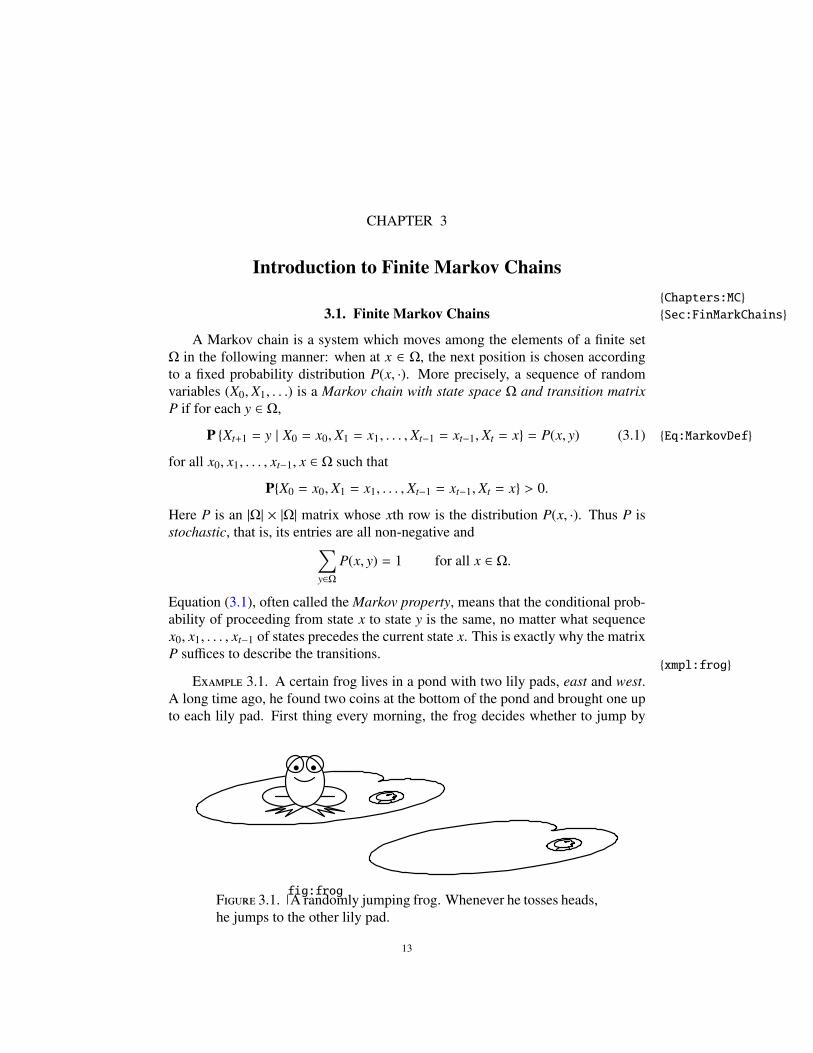
E 3.1. A certain frog lives in a pond with two lily pads, east and west.A long time ago, he found two coins at the bottom of the pond and brought one upto each lily pad. First thing every morning, the frog decides whether to jump by

F 3.1.fig:frogA randomly jumping frog. Whenever he tosses heads,

he jumps to the other lily pad.

13

14 3. INTRODUCTION TO FINITE MARKOV CHAINS

tossing the current lily pad’s coin. If the coin lands heads up, he jumps to the otherlily pad. If the coin lands tails, he remains where he is.

Let Ω = e,w, and let (X0, X1, . . . ) ∈ ΩZ+

be the sequence of lily pads occu-pied by the frog on Sunday, Monday,. . .. Given the source of the coins, we shouldnot assume that they are fair! Say the coin on the east pad has probability p oflanding heads up, while the coin on the west pad has probability q of landing headsup. The frog’s rules for jumping imply that if we set

P =(

P(e, e) P(e,w)P(w, e) P(w,w)

)=

(1 − p p

q 1 − q

), (3.2)Eq:FrogMatrix

then (X0, X1, . . . ) is a Markov chain with transition matrix P. Note that the firstrow of P is the conditional distribution of Xt+1, given that Xt = e, while the secondrow is the conditional distribution of Xt+1, given that Xt = w.

If the frog spends Sunday on the east pad, then when he awakens Monday, hehas probability p of moving to the west pad and probability 1− p of staying on theeast pad. That is,

PX1 = e | X0 = e = 1 − p, PX1 = w | X0 = e = p. (3.3)eq:time1

What happens Tuesday? The reader should check that, by conditioning on X1,

PX2 = e | X0 = e = (1 − p)(1 − p) + pq. (3.4)eq:time2a

While we could keep writing out formulas like (3.4), there is a more systematicapproach. Let’s store our distribution information in a row vector,

µt := (PXt = e | X0 = e, PXt = w | X0 = e) .

Our assumption that the frog starts on the east pad can now be written as µ0 = (1, 0),while (3.3) becomes µ1 = µ0P.

Multiplying by P on the right updates the distribution by another step:

µt = µt−1P for all t ≥ 1. (3.5)eq:frogmatmult

Indeed, for any initial distribution µ0,

µt = µ0Pt for all t ≥ 0. (3.6)eq:froghiordtrans

How does the distribution µt behave in the long term? Figure 3.2 suggests thatµt has a limit π (whose value depends on p and q) as t → ∞. Any such limitdistribution π must satisfy

π = πP,which implies (after a little algebra)

π(e) =q

p + q, π(w) =

pp + q

.

If we define, for t ≥ 0,∆t = µt(e) −

qp + q

,

then the sequence (∆t) satisfies (c.f. Exercise 3.2)

∆t+1 = (1 − p − q)∆t. (3.7)Eq:FrogRate

3.1. FINITE MARKOV CHAINS 15

(a) 0 10 20

0.25

0.5

0.75

1

(b)0 10 20

0.25

0.5

0.75

1

(c)

0 10 20

0.25

0.5

0.75

1

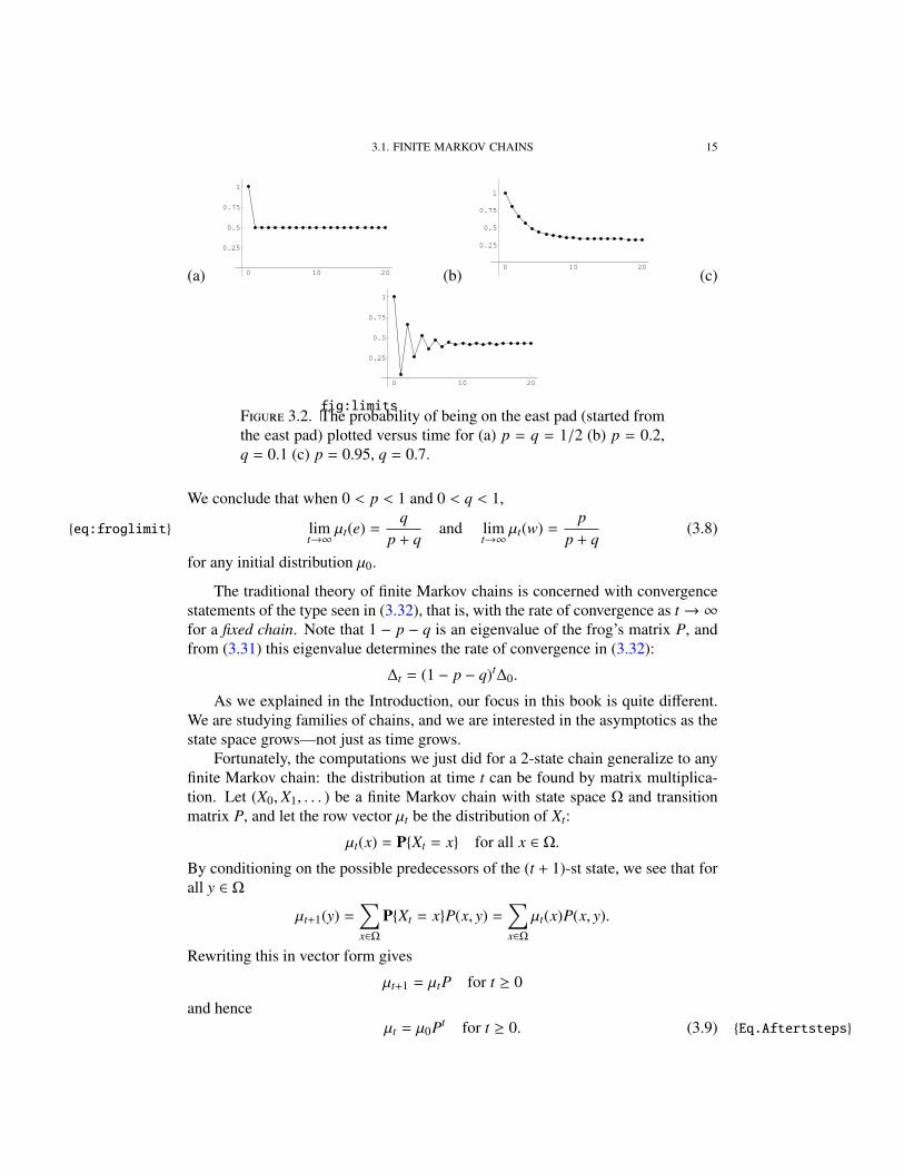
F 3.2.fig:limitsThe probability of being on the east pad (started from

the east pad) plotted versus time for (a) p = q = 1/2 (b) p = 0.2,q = 0.1 (c) p = 0.95, q = 0.7.

We conclude that when 0 < p < 1 and 0 < q < 1,

limt→∞

µt(e) =q

p + qand lim

t→∞µt(w) =

pp + q

(3.8)eq:froglimit

for any initial distribution µ0.

The traditional theory of finite Markov chains is concerned with convergencestatements of the type seen in (3.32), that is, with the rate of convergence as t → ∞for a fixed chain. Note that 1 − p − q is an eigenvalue of the frog’s matrix P, andfrom (3.31) this eigenvalue determines the rate of convergence in (3.32):

∆t = (1 − p − q)t∆0.

As we explained in the Introduction, our focus in this book is quite different.We are studying families of chains, and we are interested in the asymptotics as thestate space grows—not just as time grows.

Fortunately, the computations we just did for a 2-state chain generalize to anyfinite Markov chain: the distribution at time t can be found by matrix multiplica-tion. Let (X0, X1, . . . ) be a finite Markov chain with state space Ω and transitionmatrix P, and let the row vector µt be the distribution of Xt:

µt(x) = PXt = x for all x ∈ Ω.

By conditioning on the possible predecessors of the (t + 1)-st state, we see that forall y ∈ Ω

µt+1(y) =∑x∈Ω

PXt = xP(x, y) =∑x∈Ω

µt(x)P(x, y).

Rewriting this in vector form gives

µt+1 = µtP for t ≥ 0

and henceµt = µ0Pt for t ≥ 0. (3.9) Eq.Aftertsteps


Since we will often consider Markov chains with the same transition matrixbut different starting distributions, we introduce the notation Pµ and Eµ for proba-bilities and expectations given that µ0 = µ. Most often, the initial distribution willbe concentrated at a single definite starting state, x; we denote this distribution byδx:

δx(y) =

1 y = x,0 y , x.

We write simply Px and Ex for Pδx and Eδx , respectively.Using these definitions and (3.9) shows that

PxXt = y = (δxPt)(y) = Pt(x, y).

That is, the probability of moving in t steps from x to y is given by the (x, y)-thentry of Pt. (We call these entries the t-step transition probabilities.)

R. The way we constructed the matrix P has forced us to treat distribu-tions as row vectors. In general, if the chain has distribution µ at time t, then it hasdistribution µP at time t + 1. Multiplying a row vector by P on the right takes youfrom today’s distribution to tomorrow’s distribution.

What if we multiply a column vector f by P on the left? Think of f as functionon the state spaceΩ (for the frog of Example 3.1, f (x) might be the average numberof flies the frog catches per day at lily pad x). Consider the x-th entry of theresulting vector:

P f (x) =∑

y

P(x, y) f (y) =∑

y

f (y)PxX1 = y = Ex( f (X1)).

That is, the x-th entry of P f tells us the expected value of the function f at tomor-row’s state, given that we are at state x today. Multiplying by column vector by Pon the left takes us from a function to the expected value of that function tomorrow.

3.2. Simulating a Finite Markov ChainSec:SimMC

In Chapter 2, we discussed methods for sampling from various interesting dis-tributions on finite sets, given the ability to produce certain simple types of randomvariables—coin flips, or uniform samples from the unit interval, say. It is natural toask: how can we sample from the distribution of a Markov chain which has beenrun for many steps?

One possible method would be to explicitly compute the vector µ0Pt, then useone of the methods from Chapter 2 to sample from this distribution. If our statespace is even moderately large, this method will be extremely inefficient, sinceit requires us to raise the |Ω| × |Ω| matrix P to a large power. There is an evenmore elementary problem, however: for many chains we study (and would like tosimulate), we don’t even know |Ω|!

Fortunately, generating a trajectory of a Markov chain can be done one step ata time. Let’s look at a simple example.

3.2. SIMULATING A FINITE MARKOV CHAIN 17

F 3.3.Fig:CycleRandom walk on Z10 is periodic, since every step

goes from an even state to an odd state, or vice-versa. Randomwalk on Z9 is aperiodic.

Xmpl:NcycleE 3.2 (Random walk on the n-cycle). Let Ω = Zn = 0, 1, . . . , n − 1,

the set of remainders modulo n. Consider the transition matrix

P( j, k) =

1/2 if k ≡ j + 1 (mod n),1/2 if k ≡ j − 1 (mod n),0 otherwise.

(3.10)

The associated Markov chain (Xt) is called random walk on the n-cycle. The statescan be envisioned as equally spaced dots arranged in a circle (see Figure 3.3). Ateach time, the walker must either go one step clockwise, or one step counterclock-wise.

That description in words translates neatly into a simulation method. LetZ1,Z2, . . . be a sequence of independent and identically distributed random vari-ables, each of which is equally likely to be +1 or −1. Let’s require that our walkerstarts at 0, i.e. that X0 = 0. Then for each t ≥ 0 set

Xt+1 = Xt + Zt mod n. (3.11) eq:randmapxmpl

The resulting sequence of random variables X0, X1, . . . is clearly a Markov chainwith transition matrix P.

More generally, we define a random mapping representation of a Markov chainon state space Ω with transition matrix P to consist of a function f : Ω × Λ → Ωsuch that for some sequence of independent and identically distributed randomvariables Z0,Z1, . . . , each of which takes values in the set Λ,

X0, f (X0,Z0), f (X1,Z1), f (X2,Z2), . . .

is a Markov chain with transition matrix P. The function f takes in the currentstate and some new random information, and from that information determines thenext state of the chain. More explicitly, if we are at state x ∈ Ω at time t, and ourauxiliary randomness-generating device outputs z ∈ Λ, then the next state of thechain will be f (x, z):

(Xt = x and Zt = z)⇒ Xt+1 = f (x, z).


In the example above, Λ = 1,−1, each Zi is uniform on Λ, and

f (x, z) = x + z mod n.

P 3.3. Every transition matrix on a finite state space has a randommapping representation.

P. Let P be the transition matrix of a Markov chain with state space Ω =x1, . . . , xn. Take Λ = [0, 1]; our auxiliary random variables Z1,Z2, . . . will beuniformly chosen in this interval. To determine the function f : Ω × Λ → Ω, weuse the method of Exercise 2.9 to simulate the discrete distributions P(x j, ·). Morespecifically, set F j,k =

∑ki=1 P(x j, xi) and define

f (x j, z) := xk when F j,k−1 < z ≤ F j,k.

Note that, unlike transition matrices, random mapping representations are farfrom unique. For instance, replacing the f (x, z) in the previous proof with f (x, 1−z)yields another representation.

Random mapping representations are crucial for simulating large chains. Theycan also be the most convenient way to describe a chain. We will often give rulesfor how a chain proceeds from state to state, using some “extra” randomness todetermine where to go next; such discussions are implicit random mapping repre-sentations. Finally, random mapping representations provide a way to coordinatetwo (or more) chain trajectories, as we can simply use the same sequence of aux-iliary random variables to determine updates. This technique will be exploited inChapter 6, on coupling.

3.3. Irreducibility and AperiodicitySec:IrrAper

We now make note of two simple properties possessed by most interestingchains. Both will turn out to be necessary for the Convergence Theorem (Theorem5.6) to be true.

A chain P is called irreducible if for any two states x, y ∈ Ω, there existsan integer t (possibly depending on x and y) such that Pt(x, y) > 0. This meansthat it is possible to get from any state to any other state using only transitions ofpositive probability. We will generally assume that the chains under discussion areirreducible. (Checking that specific chains are irreducible can be quite interesting;see, for instance, Sections 4.4 and 4.7. See Section 3.7 for a discussion of all theways in which a Markov chain can fail to be irreducible.)

The chain P will be called aperiodic if gcdt : Pt(x, x) > 0 = 1 for all x ∈ Ω.If a chain is not aperiodic, we call it periodic.

If P is aperiodic and irreducible, then there is an integer r so that Pr(x, y) > 0for all x, y, ∈ Ω. (See Exercise 3.3.)

According to our definition, a chain in which all paths from x0 to x0 have evenlength is periodic. In such a chain, the states lying on x0–x0 paths can be splitinto those at even distance from x0 and those at odd distance from x0; all allowedtransitions go from one class to the other. No matter how many steps the chain

3.4. RANDOM WALKS ON GRAPHS 19

started at x0 takes, the distribution at a particular instant will never be spread overall the states. The best we can hope for is that the distribution will alternate betweenbeing nearly uniform on the “even” states, and nearly uniform on the “odd” states.Of course, if gcdt : Pt(x, x) > 0 > 2, the situation can be even worse!

Fortunately, a simple modification can repair periodicity problems. Given anarbitrary transition matrix P, let Q = I+P

2 (here I is the |Ω| × |Ω| identity matrix).(One can imagine simulating Q as follows: at each time step, flip a fair coin. Ifit comes up heads, take a step in P; if tails, then stay at the current state.) SinceQ(x, x) > 0 for all x ∈ Ω, the transition matrix Q is aperiodic. We call Q a lazyversion of P. It will often be convenient to analyze lazy versions of chains.

Xmpl:NcyclePerE 3.4 (The n-cycle, revisited). Recall random walk on the n-cycle, de-

fined in Example 3.2. For every n ≥ 1, random walk on the n-cycle is irreducible.Random walk on any even-length cycle is periodic, since gcdt : Pt(x, x) >

0 = 2 (see Figure 3.3). Random walk on an odd-length cycle is aperiodic.The transition matrix for lazy random walk on the n-cycle is

Q( j, k) =

1/4 if k ≡ j + 1 (mod n),1/2 if k ≡ j (mod n),1/4 if k ≡ j − 1 (mod n),0 otherwise.

(3.12)

Lazy random walk on the n-cycle is both irreducible and aperiodic for every n.

3.4. Random Walks on GraphsSec:RWG

The random walk on the n-cycle, shown in Figure 3.3, is a simple case of animportant type of Markov chain.

A graph G = (V, E) consists of a vertex set V and an edge set E, where theelements of E are unordered pairs of vertices: E ⊂ x, y : x, y ∈ V, x , y. We canthink of V as a set of dots, where two dots x and y are joined by a line if and only ifx, y is an element of the edge set. When x, y ∈ E we write x ∼ y and say that yis a neighbor of x (and also that x is a neighbor of y.) The degree deg(x) of a vertexx is the number of neighbors of x.

Given a graph G = (V, E), we can define simple random walk on G to be theMarkov chain with state space V and transition matrix

P(x, y) =

1deg(x) if y ∼ x,

0 otherwise.(3.13) Eq:SRW

That is to say, when the chain is at vertex x, it examines all the neighbors of x,picks one uniformly at random, and moves to the chosen vertex.

E 3.5. Consider the graph G shown in Figure 3.4. The transition matrix


1

2

3

4

5

F 3.4.fig:SRWAn example of a graph with vertex set 1, 2, 3, 4, 5

and 6 edges.

of simple random walk on G is

P =

0 12

12 0 0

13 0 1

313 0

14

14 0 1

414

0 12

12 0 0

0 0 1 0 0

.

We will say much, much more about random walks on graphs throughout thisbook—but especially in Chapter 10.

3.5. Stationary DistributionsSec:StatDist

3.5.1. Definition. We saw in Example 3.1 that a distribution π onΩ satisfying

π = πP (3.14)Eq:StationaryEq

can have another interesting property: in that case, π was the long-term limitingdistribution of the chain. We call a probability π satisfying (3.14) a stationarydistribution of the Markov chain. Clearly, if π is a stationary distribution and µ0 = π(i.e. the chain is started in a stationary distribution), then µt = π for all t ≥ 0.

Note that we can also write (3.14) elementwise: an equivalent formulation is

π(y) =∑x∈Ω

π(x)P(x, y) for all y ∈ Ω. (3.15)Eq:StationarySystem

Example:PiForSRWE 3.6. Consider simple random walk on a graph G = (V, E). For any

vertex y ∈ V , ∑x∈V

deg(x)P(x, y) =∑x∼y

deg(x)deg(x)

= deg(y). (3.16)

To get a probability, we simply normalize by∑

y∈V deg(y) = 2|E| (a fact you shouldcheck). We conclude that

π(y) =deg(y)2|E|

for all y ∈ Ω,

the probability measure proportional to the degrees, is always a stationary distribu-tion for the walk. For the graph in Figure 3.4,

π =(

212 ,

312 ,

412 ,

212 ,

112

).

3.5. STATIONARY DISTRIBUTIONS 21

If G has the property that every vertex has the same degree d, we call G d-regular.In this case 2|E| = d|V | and the uniform distribution π(y) = 1/|V | for every y ∈ V isstationary.

Our goal for the rest of this chapter and the next is to prove a general yet pre-cise version of the statement that “finite Markov chains converge to their stationarydistributions.” In this section we show that, under mild restrictions, stationary dis-tributions exist and are unique. Our strategy of building a candidate distribution,then verifying that it has the necessary properties, may seem cumbersome. How-ever, the tools we construct here will be applied many other places.

Sec:FirstReturn3.5.2. Hitting and first return times. Throughout this section, we assume

that the Markov chain X0, X1, . . . under discussion has finite state space Ω andtransition matrix P. For x ∈ Ω, define the hitting time for x to be

τx := mint ≥ 0 : Xt = x,

the first time at which the chain visits state x. For situations where only a visit to xat a positive time will do, we also define

τ+x := mint ≥ 1 : Xt = x.

When X0 = x, we call τ+x the first return time.lem:firstreturnintegrable

L 3.7. For any states x and y of an irreducible aperiodic chain, Ex(τ+y ) <∞.

P. By Exercise 3.3, there exists an r such that every entry of Pr is positive.Let ε = minz,w∈Ω Pr(z,w) be its smallest entry. No matter the value of Xt, theprobability of hitting state y at time t+r is at least ε. Thus, for k ≥ 0, the probabilitythat the chain has not arrived at y by time kr is no larger than the probability that kindependent trials, each with success probability ε, all fail:

Pxτ+y > kr ≤ PxXr , y, X2r , y, . . . , Xkr , y ≤ (1 − ε)k. (3.17) eq:everyrth

See Exercise 3.12 to complete the proof.

3.5.3. Existence of a stationary distribution. The Convergence Theorem(Theorem 5.6 below) implies that the “long-term” fractions of time a finite aperi-odic Markov chain spends in each state coincide with the chain’s stationary distri-bution. We, however, have not yet demonstrated that stationary distributions exist!To build a candidate distribution, we consider a sojourn of the chain from somearbitrary state z back to z. Since visits to z break up the trajectory of the chaininto identically distributed segments, it should not be surprising that the averagefraction of time per segment spent in each state y coincides with the “long-term”fraction of time spent in y.

Prop:PiExistsP 3.8. Let P be the transition matrix of an irreducible Markov chain.

Then there exists a probability distribution π on Ω such that π = πP.


P. Let z ∈ Ω be an arbitrary state of the Markov chain. We will closelyexamine the time the chain spends, on average, at each state in between visits to z.Hence define

π(y) := Ez(number of visits to y before returning to z)

=

∞∑t=0

PzXt = y, τ+z > t.(3.18) eq:pitildedefn

By Exercise 3.13, π(y) < ∞ for all y ∈ Ω. Let’s try checking whether π is stationary,starting from the definition:

∑x∈Ω

π(x)P(x, y) =∑x∈Ω

∞∑t=0

PzXt = x, τ+z > tP(x, y). (3.19)eq:tildesum

Now reverse the order of summation in (3.19). After doing so, we can use theMarkov property to compute the sum over x. Essentially we are shifting by onethe time slots checked, while at the same time shifting the state checked for by onestep of the chain—from x to y:

∞∑t=0

∑x∈Ω

PzXt = x, τ+z ≥ t + 1P(x, y) =∞∑

t=0

PzXt+1 = y, τ+z ≥ t + 1 (3.20)

=

∞∑t=1

PzXt = y, τ+z ≥ t. (3.21)eq:almostthere

The expression in (3.21) is very similar to (3.18), so we’re almost done. In fact,

∞∑t=1

PzXt = y, τ+z ≥ t = π(y) − PzX0 = y, τ+z > 0 +∞∑

t=1

PzXt = y, τ+z = t (3.22)

= π(y) − PzX0 = y + PzXτ+z = y. (3.23)eq:negligibledifference

Now consider two cases:

y = z: Since X0 = z and Xτ+z = z, the two last terms of (3.23) are both 1, andthey cancel each other out.

y , z: Here both terms are 0.

Finally, to get a probability measure, we normalize by∑

x π(x) = Ez(τ+z ):

π(x) =π(x)

Ez(τ+z )satisfies π = πP. (3.24)Eq:pi

R. The computation at the heart of the proof of Proposition 3.8 can begeneralized. The argument we give above works whenever X0 = z is a fixed stateand the stopping time τ satisfies both Pzτ < ∞ = 1 and Pzτ = z = 1.

3.6. REVERSIBILITY AND TIME REVERSALS 23

Sec:StatUnique3.5.4. Uniqueness of the stationary distribution. Earlier this chapter we

pointed out the difference between multiplying a row vector by P on the right anda column vector by P on the left: the former advances a distribution by one stepof the chain, while the latter gives the expectation of a function on states, one stepof the chain later. We call distributions invariant under right multiplication by Pstationary. What about functions that are invariant under left multiplication?

Call a function h : Ω→ R harmonic at x if

h(x) =∑y∈Ω

P(x, y)h(y). (3.25) Eq:HarmonicDefn

A function is harmonic on D ⊂ Ω if it is harmonic at every state x ∈ D. If h isregarded as a column vector, then a function which is harmonic on all ofΩ satisfiesthe matrix equation Ph = h.

Lem:LiouvilleL 3.9. A function h which is harmonic at every point of Ω is constant.

P. Since Ω is finite, there must be a state x0 such that h(x0) = M is maxi-mal. If for some state z such that P(x0, z) > 0 we have h(z) < M, then

h(x0) = P(x0, z)h(z) +∑y,z

P(x0, y)h(y) < M, (3.26)

a contradiction. It follows that h(z) = M for all states z such that P(x0, z) > 0.For any y ∈ Ω, irreducibility implies that there is a sequence x0, x1, . . . , xn = y

with P(xi, xi+1) > 0. Repeating the argument above tells us that h(y) = h(xn−1) =· · · = h(x0) = M. Thus h is constant.

Cor:StatDistUniqueC 3.10. Let P be the transition matrix of an irreducible Markov chain.

There exists a unique probability distribution π satisfying π = πP.

P. While proving Proposition 3.8, we constructed one such measure. Lemma 3.9implies that the kernel of P − I has dimension 1, so the column rank of P − I is|Ω|−1. The row rank equals column rank (equals rank), so the row-vector equationν = νP also has a one-dimensional space of solutions. This space contains onlyone vector whose entries sum to 1.

R. Another proof of Corollary 3.10 follows from the Convergence The-orem (Theorem 5.6, proved below).

3.6. Reversibility and time reversalsSec:Reversibility

Suppose a probability π on Ω satisfies

π(x)P(x, y) = π(y)P(y, x). (3.27) Eq:DetailedBalance

Exercise 3.22 asks you to check that π is then stationary for P. Furthermore, when(3.27) holds,

π(x0)P(x0, x1) · · · P(xn−1, xn) = π(xn)P(xn, xn−1) · · · P(x1, x0). (3.28) Eq:Reversed

We can rewrite (3.28) in the following suggestive form:

PπX0 = x0, . . . , Xn = xn = PπX0 = xn, X1 = xn−1, . . . , Xn = x0, (3.29) Eq:Reversed2


In words: when a chain satisfying (3.27) is run in stationarity, the distribution offinite segments of trajectory is the same no matter whether we run time backwardsor forwards. For this reason, a chain satisfying (3.27) is called reversible. Theequations (3.27) are called the detailed balance equations.

The time-reversal of a Markov chain with transition matrix P and stationarydistribution π is the chain with matrix

P(x, y) :=π(y)P(y, x)

π(x). (3.30)Eq:ReversedMatrix

Exercise 7.6 shows that the terminology “time-reversal” is reasonable. (Notethat when a chain is reversible, as defined in Section 3.6, then P = P.)

3.7. Classifying the States of a Markov Chain*sec:classification

We will occasionally need to study chains which are not irreducible—see, forinstance, Sections 4.1, 4.2 and 4.3.3. In this section we describe a way to clas-sify the states of a Markov chain; this classification clarifies what can occur whenirreducibility fails.

Let P be the transition matrix of a Markov chain on a finite state space Ω.Given x, y ∈ Ω, we say that x sees y, and write x → y, if there exists an r > 0 suchthat

Pr(x, y) > 0. That is, x sees y if it’s possible for a trajectory of the chain toproceed from x to y. We say that x communicates with y, and write x ↔ y, if andonly if x→ y and y→ x.

The equivalence classes under↔ are called communication classes. For x ∈ Ω,let [x] denote the communication class of x.

E 3.11. When P is irreducible, all the states of the chain lie in a singlecommunication class.

E 3.12. When a communication class consists of a single state z ∈ Ω, itfollows that P(z, z) = 1 and we call z an absorbing state. Once a trajectory arrivesat z, it is “absorbed” there and can never leave.

It follows from Exercise 3.24(c) that every chain trajectory follows a weakly in-creasing path in the partial order on communication classes. Once the chain arrivesin a class that is maximal in this order, it stays there forever. See Exercise 18.8,which connects this structure to the concepts of recurrence and transience definedin Chapter 18.

3.8. ProblemsExer:frogstate

E 3.1. Can you tell what time of day is shown in Figure 3.1? What arethe frog’s plans? [S]

ex:froglimitE 3.2. Consider the jumping frog chain of Example 3.1, whose transi-

tion matrix is given in (3.2). Assume that our frog begins hopping from an arbitrarydistribution µ0 on e,w.

3.8. PROBLEMS 25

(a) Define, for t ≥ 0,

∆t = µt(e) −q

p + q.

Show that∆t+1 = (1 − p − q)∆t. (3.31) Eq:FrogRate

(b) Conclude that when 0 < p < 1 and 0 < q < 1,

limt→∞

µt(e) =q

p + qand lim

t→∞µt(w) =

pp + q

(3.32) eq:froglimit

for any initial distribution µ0.Exer:Aperiodic

E 3.3. Show that when P is aperiodic and irreducible, there exists aninteger r such that Pr(x, y) > 0 for all x, y ∈ Ω.

ex:oddcycleE 3.4. Let P be the transition matrix of random walk on the n-cycle,

where n is odd. Find the smallest value of t such that Pt(x, y) > 0 for all states xand y.

Exer:ConnectedE 3.5. A graph G is connected when any two vertices x and y of G can

be connected by a path x = x0, x1, . . . , xk = y of vertices such that xi ∼ xi+1, for0 ≤ i ≤ k − 1. Show that random walk on G is irreducible if and only if G isconnected.

Exer:TreeTFAE

E 3.6. We define a graph to be a tree if it is connected, but contains nocycles. Prove that the following statements about a graph T with n vertices and medges are equivalent:(a) T is a tree.(b) T is connected and m = n − 1.(c) T has no cycles and m = n − 1.

Exer:TreeBasicsE 3.7. Let T be a tree.

(a) Prove that T contains a leaf, that is, a vertex of degree 1.(b) Prove that between any two vertices in T there is a unique path.

Exer:Tree3ColIrrE 3.8. Let T be a tree. Show that the graph whose vertices are proper

3-colorings of T , and whose edges are pairs of colorings which differ at only asingle vertex, is connected. [S]

Exer:PermParityE 3.9. Consider the following natural (if apparently slow) method of

shuffling cards: at each point in time, a pair of distinct cards is chosen, and thepositions of those two cards are switched. Mathematically, this corresponds to thefollowing Markov chain: make the state space Ω = S n, the set of all permutationsof [n], and set

P(σ1, σ2) =

1/(n2

)σ2 = σ1(i j) for some transposition (i j),

0 otherwise.

(a) Show that this Markov chain is irreducible, but periodic.


1 2 3 4

5 6 7 8

9 10 11 12

13 15 14

F 3.5.Fig:fifteenThe “fifteen puzzle”.

(b) Modify the shuffling technique so that the two cards to be exchanged are cho-sen independently and uniformly at random (and if the same card is chosentwice, nothing is done to the deck). Compute the transition probabilities forthe modified shuffle, and show that it is both irreducible and aperiodic.

Exer:fifteenE 3.10. The long-notorious Sam Loyd “fifteen puzzle” is shown in Fig-

ure 3.5. It consists of 15 tiles, numbered with the values 1 through 15, sitting in a4 by 4 grid; one space is left empty. The tiles are in order, except that tiles 14 and15 have been switched. The only allowed moves are to slide a tile adjacent to theempty space into the empty space.

Is it possible, using only legal moves, to switch the positions of tiles 14 and15, while leaving the rest of the tiles fixed?(a) Show that the answer is “no.”(b) Describe the set of all configurations of tiles that can be reached using only

legal moves.[S]

Exer:SymmTransMatE 3.11. Let P be a transition matrix satisfying P(x, y) = P(y, x) for all

states x, y ∈ Ω. Show that the uniform distribution on Ω is stationary for P.Exer:FirstReturnIntegrable

E 3.12.(a) Prove that if Y is a positive integer-valued random variable, then E(Y) =∑

t≥0 PY > t.(b) Use (a) and (3.17) to finish the proof of Lemma 3.7.

[S]Exer:RetTimeIrr

E 3.13. Prove that if P is irreducible (but not necessarily aperiodic),then Ex(τ+y ) < ∞. [S]

Exer:TwoStepsRevE 3.14. Let P be a transition matrix which is reversible with respect to

the probability distribution π on Ω. Show that the transition matrix P2 correspond-ing to two steps of the chain is also reversible with respect to π. [S]

Exer:StatDistPosE 3.15. Let π be a stationary distribution for an irreducible transition

matrix P. Prove that π(x) > 0 for all x ∈ Ω.

E 3.16. Check carefully that equation (3.18) is true.ex:periodicstatdist

E 3.17. Let P be the transition matrix of a chain and let Q = I+P2 .

3.8. PROBLEMS 27

(a) Show that for any distribution µ on Ω, µ = µP if and only if µ = µQ.(b) Show that P has a unique stationary distribution if and only if Q does.

Exer:BolzWeierStatDistE 3.18. Here we outline another proof, more analytic, of the existence

of stationary distributions. Let P be the transition matrix of a Markov chain onstate space Ω. For an arbitrary initial distribution µ on Ω and n > 0, define thedistribution νn by

νn =1n

(µ + µP + · · · + µPn−1

).

(a) Show that for any x ∈ Ω and n > 0,

|νnP(x) − νn(x)| ≤2n.

(b) Show that there exists a subsequence (νnk )k≥0 such that limk →∞ vnk (x) existsfor every x ∈ X.

(c) For x ∈ Ω, define ν(x) = limk →∞ vnk (x). Show that ν is a stationary distributionfor P.

[S]

E 3.19. Let P be the transition matrix of a Markov chain with statespace X. Let ∆ ⊂ X be a subset of the state space, and assume h : Ω → R is afunction harmonic at all states x < ∆.

Prove that if h(y) = maxx∈Ω h(x), then y ∈ ∆. (Note: this is a discrete versionof a maximum principle.)

Exer:RetTimeE 3.20. Show that for any state x of an irreducible chain, π(x) = 1

Ex(τ+x ) .

E 3.21. Check that for any graph G, the simple random walk on Gdefined by (3.13) is reversible.

Exer:RevImpliesStatE 3.22. Show that when π satisfies (3.27), then π also satisfies (3.14),

i.e. π is stationary for P.

The following exercises concern the material in Section 3.7.Exer:ClassEquiv

E 3.23. Show that↔ is an equivalence relation on Ω.Exer:ClassPartialOrder

E 3.24. The relation “sees” can be lifted to communication classes bydefining [x]→ [y] if and only if x→ y.(a) Show that→ is a well-defined relation on the communication classes.(b) Show that→ is a partial order on communication classes.(c) Show that if, in some trajectory (Xt) of the underlying Markov chain, Xr = x

and Xs = y, where r < s, then [x]→ [y].

R. It is certainly possible for the partial order constructed in Exercise 3.24(b)above to be trivial, in the sense that no class can see any other! In this case the un-derlying Markov chain consists of non-interacting sets of mutually communicatingstates; any trajectory is confined to a single communication class.


3.9. Notes

The right-hand side of (3.1) does not depend on t either. We take this as partof the definition of a Markov chain; be warned that other authors sometimes singlethis out as a special case, which they call time homogeneous. (This simply meansthat the transition matrix is the same at each step of the chain. It is possible to givea more general definition in which the transition matrix depends on t. We will notconsider such chains in these notes.)

Aldous and Fill (in progress, Chapter 2, Proposition 4) present a version of thekey computation for Proposition 3.8 which requires only that the chain be startedin the same distribution as the stopping time ends. We have essentially followedtheir proof.

The standard approach to demonstrating that irreducible aperiodic Markovchains have unique stationary distributions is through the Perron-Frobenius the-orem. See, for instance, Karlin and Taylor (1975) or Seneta (2006).

http://www.stat.berkeley.edu/~aldous/RWG/book.html

CHAPTER 4

Some Interesting Markov Chains

Ch:ClassicHere we present several basic and important examples of Markov chains. Each

chain results from a situation that occurs often in other problems, and the resultswe prove in this chapter will be used in many places throughout the book.

This is also the only chapter in the book where the central chains are not alwaysirreducible. Indeed, two of our examples, gambler’s ruin and coupon collecting,both have absorbing states (for each we examine closely how long it takes to beabsorbed).

4.1. Gambler’s RuinSec:Gambler

Consider a gambler betting on the outcome of a sequence of independent faircoin tosses. If the coin comes up heads, she adds one dollar to her purse; if the coinlands tails, she loses one dollar. If she ever reaches a fortune of n dollars, she willstop playing. If her purse is ever empty, then she must stop betting.

This situation can be modeled by a random walk on a path with vertices 0, 1, . . . , n.At all interior vertices, the walk is equally likely to go up by 1 or down by 1. Onceit arrives at 0 or n, however, it stays forever. In the language of Section 3.7, thestates 0 and n are absorbing.

There are two questions that immediately come to mind: how long will it takefor the gambler to arrive at one of the two possible fates? And what are the proba-bilities of the two possibilities?

Prop:GamblerP 4.1. Assume that a gambler making fair unit bets on coin flips will

abandon the game when his fortune falls to 0 or rises to n. Let Xt be gambler’sfortune at time t and let τ be the time required to be absorbed at one of 0 or n.Assume that X0 = k, where 0 ≤ k ≤ n. Then:

Ek(τ) = k(n − k), (4.1) Eq:GRExpTime

PkXτ = n = k/n. (4.2) Eq:GRProb

n0 1 2

F 4.1. How long until the walker reaches either 0 or n? Andwhat is the probability of each?

Fig:GamblersRuin

29

30 4. SOME INTERESTING MARKOV CHAINS

P. To solve for the value Ek(τ) for a specific k, it is easiest to consider theproblem of finding the values Ek(τ) for all k = 0, 1, . . . , n. To this end, write fkfor the expected time Ek(τ) started at position k. Clearly, f0 = fn = 0; the walk isstarted at one of the absorbing states. For 1 ≤ k ≤ n − 1, it’s true that

fk =12

(1 + fk+1) +12

(1 + fk−1) (4.3)Eq:GRR

Why? When the first step of the walk increases the gambler’s fortune, then theconditional expectation of τ is 1 plus the expected additional time needed. Theexpected additional time needed is fk+1, because the walk is now at position k + 1.Parallel reasoning applies when the gambler’s fortune first decreases.

Exercise 4.1 asks you to solve this system of equations, completing the proofof Equation 4.1.

Equation 4.2 is even simpler. Again we try to solve for all the values at once.Let pk be the probability that the gambler reaches a fortune of n before ruin, giventhat she starts with k dollars. Then p0 = 0 and pn = 1, while

pk =12

pk−1 +12

pk+1, for 1 ≤ k ≤ n − 1. (4.4)Eq:GamblerResult

Why? If the gambler is at one end or the other, she stays there—the outcome neverchanges. If she’s in between, then the result of the next bet is equally likely toincrease her fortune by 1, or decrease it by 1.

Clearly the values pk must be evenly spaced between 0 and 1, and thus pk =

k/n.

R. See Chapter 10 for powerful generalizations of the simple methodswe have just applied.

4.2. Coupon CollectingSec:CouponCollecting

A card company issues baseball cards, each featuring a single player. Thereare n players total, and a collector desires a complete set. We suppose each cardhe acquires is equally likely to be each of the n players. How many cards must heobtain so that his collection contains all n players?

It may not be obvious why this is a Markov chain. Let Xt denote the numberof different players represented among the collector’s first t cards. Clearly X0 = 0.When the collector has cards of k different types, there are n − k types missing. Ofthe n possibilities for his next card, only n − k will expand his collection. Hence

PXt+1 = k + 1 | Xt = k =n − k

n,

and

PXt+1 = k | Xt = k =kn.

Every trajectory of this chain is non-decreasing. Once the chain arrives at state n(corresponding to a complete collection), it is absorbed there. We are interested inthe number of steps required to reach the absorbing state.

4.3. URN MODELS 31

Prop:CouponExpectedP 4.2. Consider a collector attempting to collect a complete set of

cards. Assume that each new card is chosen uniformly and independently from theset of n possible types, and let τ be the (random) number of cards collected whenthe set first contains every type. Then

E(τ) = nn∑

k=1

1k.

P. The expectation E(τ) can be computed by writing τ as a sum of geo-metric random variables. Let τk be the total number of cards accumulated whenthe collection first contains k distinct players. Then

τ = τn = τ1 + (τ2 − τ1) + · · · + (τn − τn−1). (4.5)

Furthermore, τk − τk−1 is a geometric random variable with success probability(n− k+1)/n: after collecting τk−1 cards, n− k+1 of the n players are missing fromthe collection. Each subsequent card drawn has the same probability (n − k − 1)/nof being a player not already collected, until such a card is finally drawn. ThusE(τk − τk−1) = n/(n − k + 1) and

E(τ) =n∑

k=1

E(τk − τk−1) = nn∑

k=1

1n − k + 1

= nn∑

k=1

1k. (4.6) Eq:CCExp

While Proposition 4.2 is simple and vivid—you should not forget the argument!—we will generally need to know more in about the distribution of τ in future applica-tions. Recall that

∑nk=1

1k ≈ log n (see Exercises 4.5 for more detail). The following

estimate says that T is unlikely to be much larger than its expected value.Prop:CouponTail

P 4.3. Let τ be a coupon collector random variable, as in Proposi-tion 4.2. Then for any c > 0

Pτ > n log n + cn ≤ e−c.

P. Let Ai be the event that the ith player does not appear among the firstn log n + cn cards drawn. Then

Pτ > n log n + cn = P n⋃

i=1

Ai

≤ n∑i=1

P(Ai)

=

n∑i=1

(1 −

1n

)n log n+cn

≤ n exp(−

n log n + cnn

)= e−c. (4.7) Eq:CouponTail

4.3. Urn ModelsSec:UrnsSec:BLUrn

4.3.1. The Bernoulli-Laplace model.


Sec:Ehrenfest4.3.2. The Ehrenfest urn model and the hypercube. Suppose n balls are

distributed among two urns, I and II. At each move, a ball is selected at randomand transferred from its current urn to the other urn. If (Xt) is the number of ballsin urn I at time t, then the transition matrix for (Xt) is

P( j, k) =

n− j

n if k = j + 1,jn if k = j − 1,0 otherwise.

(4.8)Eq:EhrenTM

Thus, the chain lives on Ω = 0, 1, 2, . . . , n, moving by ±1 on each move, andbiased towards the middle of the interval.

Exercise 4.6 asks you to check that the stationary distribution is binomial withparameters n and 1/2.

The Ehrenfest urn is a projection of the random walk on the n-dimensional hy-percube. The n-dimensional hypercube is the graph which has vertex set 0, 1n andhas edges connecting vectors which differ in exactly one coordinate. See Figure 4.2for an illustration of the 3-dimensional hypercube.

000 100

010 110

001 101

011 111

F 4.2. The 3-dimensional hypercube.Fig:HypercubeA

The simple random walk on 0, 1n moves from a vertex (x1, x2, . . . , xn) bychoosing a coordinate j ∈ 1, 2, . . . , n uniformly at random, and setting the newstate equal to (x1, . . . , 1 − x j, . . . , xn). That is, the bit at the chosen coordinate isflipped.

It will be convenient to often consider instead the lazy random walker. Thiswalker remains at its current position with probability 1/2, and moves as abovewith probability 1/2. This chain can be realized by choosing a coordinate uni-formly at random and refreshing the bit at this coordinate by replacing it with anunbiased random bit independent of everything.

Define the Hamming weight W(x) of a vector x = (x1, . . . , xn) ∈ 0, 1n as thenumber of coordinates with value 1:

W(x) =n∑

j=1

x j. (4.9)Eq:HammingDefn

Let (Xt) be the simple random walk on 0, 1n, and let Wt = W(Xt) be theHamming weight of the walker at time t.

4.4. RANDOM WALKS ON GROUPS 33

When Wt = j, the weight increments by a unit amount when one of the n − jcoordinates with value 0 is selected. Likewise, when one of the j coordinates withvalue 1 is selected, the weight decrements by one unit. From this it is clear that(Wt) is a Markov chain with transition probabilities given by (4.8).

Sec:Polya4.3.3. The Polya urn model. Consider the following process, known as Polya’s

urn. Start with an urn containing two balls, one black and one white. From thispoint on, proceed by choosing a ball at random from those already in the urn; re-turn the chosen ball to the urn and add another ball of the same color. If there arej black balls in the urn after k balls have been added (so that there are k + 2 ballstotal in the urn), then the probability another black ball is added is j/(k + 2). Thesequence of ordered pairs listing the numbers of black and white balls is a Markovchain with state space 1, 2, . . .2.

Lem:PUUniformL 4.4. Let Bk be the number of black balls in Polya’s urn after the addi-

tion of k balls. The distribution of Bk is uniform on 1, 2, . . . , k + 1.

P. Let U0,U1, . . . ,Un be independent and identically distributed randomvariables, each uniformly distributed on the interval [0, 1]. Let Lk be the numberof U1,U2, . . . ,Uk which lie to the left of U0.

The event Lk = j− 1, Lk+1 = j occurs if and only if U0 is the ( j+ 1)st small-est and Uk+1 is one of the j smallest among U0,U1, . . . ,Uk+1. There are j(k!)orderings of U0,U1, . . . ,Uk+1 making up this event; since all (k + 2)! orderingsare equally likely,

PLk = j − 1, Lk+1 = j =j(k!)

(k + 2)!=

j(k + 2)(k + 1)

. (4.10) Eq:JointLk

Clearly PLk = j − 1 = 1/(k + 1), which with (4.10) shows that

PLk+1 = j | Lk = j − 1 =j

k + 2. (4.11) Eq:Lk1

Since Lk+1 ∈ j − 1, j given Lk = j − 1,

PLk+1 = j − 1 | Lk = j − 1 =k + 2 − j

k + 2. (4.12) Eq:Lk2

Equation 4.11 and Equation 4.12 show that the sequences (Lk + 1)nk=1 and

(Bk)nk=1 have the same distribution; in particular, Lk + 1 and Bk have the same

distribution.Since the position of U0 among U0, . . . ,Uk is uniform among the k + 1

possible positions, Lk + 1 is uniform on 1, . . . , k + 1. Thus, Bk is uniform on1, . . . , k + 1.

4.4. Random Walks on GroupsSec:RWGroups

Several of the examples we have already examined and many others we willstudy in future chapters share some important symmetry properties, which wemake explicit here. Recall that a group is a set G endowed with an associativeoperation · : G ×G → G and an identity e ∈ G such that for all g ∈ G,

(i) e · g = g and g · e = g, and


(ii) there exists an inverse g−1 ∈ G for which g · g−1 = g−1 · g = e.Xmpl:SnCycleNot

E 4.5. The set Sn of all permutations of the standard n-element set1, 2, . . . , n, introduced in Section 2.4, forms a group under the operation of func-tional composition. The identity element of Sn is the identity function id(k) = k.Every σ ∈ Sn has a well-defined inverse function, which is its inverse in the group.

We will sometimes find it convenient to use cycle notation for permutations.In this notation, a string such as (abc) refers to the permutation which sends theelement a to b, the element b to c, and the element c to a. When several cyclesare written consecutively, they are performed one at a time, from right to left (as isconsistent with ordinary function composition). For example,

(13)(12) = (123)

and(12)(23)(34)(23)(12) = (14).

Given a probability measure µ on a group (G, ·), we can define a random walkon G with increment distribution µ as follows: it is a Markov chain with state spaceG and which moves by multiplying the current state on the left by a random elementof G selected according to µ. Equivalently, the transition matrix P of this chain hasentries

P(g, hg) = µ(h).

E 4.6 (The n-cycle). Let µ assign probability 1/2 to each of to 1 andn − 1 ≡ −1 (mod n) in the additive cyclic group Zn = 0, 1, . . . , n − 1. Then thesimple random walk on the n-cycle first introduced in Example 3.2 is the randomwalk on Zn with increment µ. Similarly, if ν assigns weight 1/4 to both 1 andn − 1 and weight 1/2 to 0, then lazy random walk on the n-cycle, discussed inExample 3.4, is the random walk on Zn with increment ν.

E 4.7 (The hypercube). The hypercube random walks discussed in Sec-tion 4.3.2 can be viewed as a random walks on the group Zn

2, which is the directproduct of n copies of the two-element group Z2 = 0, 1. For the simple randomwalk the increment measure is uniform on the set ei | 1 ≤ i ≤ n, where ei has a 1 inthe i-th place and 0 in all other entries. For the lazy version, the increment measuregives the vector 0 (with all zero entries) weight 1/2 and each ei weight 1/2n.

R. We are multiplying the current state by the increment on the left be-cause it is often more natural in the symmetric group, which is our most importantnon-commutative example. (For commutative examples, such as Zn or the hyper-cube, it of course doesn’t matter on which side we multiply.)

Prop:RWGStatP 4.8. Let P be the transition matrix of a random walk on a finite

group G. Then the uniform measure on G is a stationary distribution for P.

P. Let µ be the increment distribution of the random walk, and let U de-note the uniform measure on G. For any g ∈ G,∑

h∈G

P(h, g)U(h) =1|G|

∑k∈G

P(k−1g, g) =1|G|

∑k∈G

µ(k) =1|G|= U(g).

4.4. RANDOM WALKS ON GROUPS 35

For the first equality, we reindexed by setting k = gh−1. (The key point is that, justas it is possible to step away from g using any element in the support of µ, it ispossible to arrive at G using any element in the support of µ.)

4.4.1. Generating sets and irreducibility. For a set H ⊂ G, let 〈H〉 be thesmallest group containing all the elements of H; recall that every element of 〈H〉can be written as a product of elements in H and their inverses. A set H is said togenerate G if 〈H〉 = G.

P 4.9. Let µ be a probability measure on a finite group G. Therandom walk on G with increments µ is irreducible if and only if S=g ∈ G | µ(g) >0 generates G.

P. When the random walk is irreducible, then for any a, b ∈ G there existsan r > 0 s.t. Pr(a, b) > 0. In order for this to occur, there must be a sequences1, . . . , sr ∈ G such that b = sr sr−1 . . . s1a and gi ∈ S for i = 1, . . . , r.

Now assume S generates G, and consider a, b ∈ G. Let g = ba−1. We knowthat g can be written as a word in the elements of S and their inverses. Since everyelement of G has finite order, any inverses appearing in the expression for g canbe rewritten as positive powers of elements of S . If the resulting expression isg = smsm−1 . . .1 where si ∈ S for i = 1, . . . ,m, then

Pm(a, b) = Pm(a, ga) = P(a, s1a)P(s1a, s2s1a) . . . P(sm−1 . . .1 a, ga) > 0.

Let G be a group and let J be a set which generates G. The directed Cayleygraph associated to G and J is the directed graph with vertex set G in which (v,w)is an edge if and only if v = gw for some generator g ∈ J.

We call a set J of generators of G symmetric if g ∈ J implies g−1 ∈ J. WhenJ is symmetric, all edges in the directed Cayley graph are bidirectional, and it maybe viewed as an ordinary graph.

E 4.10 (Random transpositions, version 1). A transposition is an ele-ment of Sn that interchanges two elements and leaves all others fixed. Let T ⊆ Snbe the set of all transpositions. In Section 2.4, we gave a method for generating auniform random permutation that started with the sorted sequence and used onlytranspositions. Hence 〈T 〉 = S n, and the corresponding random walk is irreducible.

Suppose that G is finite with generators g1, . . . , gn. The simple random walkon the Cayley graph of G is the random walk on G with µ taken to be the uniformdistribution on the generators.

Sec:PermParity4.4.2. Parity of permutations and periodicity. For contrast, consider the set

T ′ of all three-cycles in Sn. The set T ′ does not generate all of Sn, but we mustintroduce an important property of the permutation group Sn to see why. Given apermutation σ ∈ Sn, consider the sign of the product

M(σ) =∏

1≤i< j≤n

(σ( j) − σ(i)) .


Clearly M(id) > 0, since every term is positive. For every σ ∈ Sn and everytransposition (ab), we have

M((ab)σ) = −M(σ).

Why? We may assume that a < b. Then for every c such that a < c < b, twofactors change sign, while the single factor containing both a and b also changessign.

Call a permutation σ even if M(σ) > 0, and otherwise call σ odd. Note thata permutation is even (odd) if and only if every way of writing it as a product oftranspositions contains an even (odd) number of factors. Furthermore, under com-position of permutations, evenness and oddness follow the same rules as they dofor integer addition. Hence the set of all even permutations in S n forms a subgroup,known as the alternating group An.

4.4.3. Reversibility and random walks on groups.Sec:Transitive

4.4.4. Transitive chains. A Markov chain is called transitive if for each pair(x, y) ∈ Ω ×Ω there is a function φ = φ(x,y) mapping Ω to itself such that

φ(x) = y and P(z,w) = P(φ(z), φ(w)). (4.13)

Roughly, this mean the chain “looks the same” from any point in the state-spaceΩ.

4.5. Reflection Principles

A nearest-neighbor random walk on Z moves right and left by at most onestep on each move, and each move is independent of the past. More exactly, if (∆t)is a sequence of independent and identically distributed −1, 0, 1-valued randomvariables and Xt =

∑ts=1 ∆s, then the sequence (Xt) is a nearest-neighbor random

walk with increments (∆t).This sequence of random variables is a Markov chain with infinite state-space

Z and transition matrix

P(k, k + 1) = p, P(k, k) = r, P(k, k − 1) = q,

where p + r + q = 1.The special case where p = q = 1/2, r = 0 is called the simple random walk,

and if p = q = 1/4, r = 1/2 the chain is called the lazy simple random walk.Thm:SRWHitBound

T 4.11. If (Xt) is the simple random walk on Z and τ0 is the first timethat the walk visits 0, then for k = 1, 2, . . .,

Pkτ0 > r ≤12k√

r(4.14)Eq:SRWHitBound

We prove this by a sequence of lemmas which are of independent interest.Lem:RP0

L 4.12 (Reflection Principle). Let (Xt) be either the simple random walkor the lazy simple random walk on −B, . . . , B, and let

τ0 := mint ≥ 0 : Xt = 0

4.5. REFLECTION PRINCIPLES 37

be the first time when the walk hits 0. For k ∈ 1, 2, . . .,

Pkτ0 < r, Xr = j = PkXr = − j.

Summing over j ≥ 1 shows that

Pkτ0 < r, Xr > 0 = PkXr < 0.

P. The walker “starts afresh” from 0 when he hits 0, meaning that the walkviewed from the first time it hits zero has the same distribution as a walk startedfrom zero and is independent of the past. From this, for j = 1, 2, . . .,

Pkτ0 = s, Xr = j = Pkτ0 = sP0Xr−s = j.

The distribution of Xt is symmetric when started at 0, so the right-hand side equals

Pkτ0 = sP0Xr−s = − j = Pkτ0 = s, Xr = − j.

Summing over s < r,

Pkτ0 < r, Xr = j = Pkτ0 < r, Xr = − j = PkXr = − j.

The last equality follows since the random walk must past through 0 before hittinga negative integer.

R 4.1. There is also a simple combinatorial proof of Lemma 4.12. Thereis a one-to-one correspondence between walk paths which hit 0 before time r andare positive at time r and walk paths which are negative at time r. This is illustratedin Figure 4.3: to obtain a bijection from the former set of paths to the latter set,reflect a path after the first time it hits 0.

F 4.3. A path hitting zero and ending above zero can betransformed, by reflection, into a path ending below zero.

Fig:RP.


E 4.13 (First passage time for simple random walk). A nice applicationof Lemma 4.12 gives the distribution of τ0 when starting from 1. We have

P1τ0 = 2m + 1 = P1τ0 > 2m, X2m = 1, X2m+1 = 0= P1τ0 > 2m, X2m = 1P1X2m+1 = 0 | X2m = 1

= P1τ0 > 2m, X2m = 112.

The second to the last equality follows since the conditional probability of hitting0 at time 2m + 1, given that at time 2m the walker is at 1 and has not previouslyvisited 0, is simply the probability of moving from 1 to 0 in one move (by theMarkov property). Rewriting and using Lemma 4.12 yields

P1τ0 = 2m + 1 =12

[P1X2m = 1 − P1τ0 ≤ 2m, X2m = 1

]=

12

[P1X2m = 1 − P1X2m = −1

].

Calculating using the Binomial distribution shows that

P1τ0 = 2m + 1 =12

[(2mm

)2−2m −

(2m

m − 1

)2−2m

]=

1(m + 1)22m+1

(2mm

).

Lem:RP1L 4.14. For simple random walk or lazy simple random walk (Xt) on Z,

for k = 1, 2, . . .,Pkτ0 > r = P0−k < Xr ≤ k.

P. We can write

PkXr > 0 = PkXr > 0, τ0 ≤ r + Pkτ0 > r.

By Lemma 4.12,PkXr > 0 = PkXr < 0 + Pkτ0 > r.

By symmetry of the walk, PkXr < 0 = PkXr > 2k, and so

Pkτ0 > r = PkXr > 0 − PkXr > 2k = Pk0 < Xr ≤ 2k = P0−k < Xr ≤ k.

Lem:RP2

L 4.15. For the simple random walk (Xt) on Z,

P0Xt = k ≤3√

t. (4.15)Eq:SRWStirling

R 4.2. By applying Stirling’s formula a bit more carefully than we do inthe proof below, one can see that in fact

P0X2r = 2k =1√πr

[1 + o(1)]

when is k not too far away from 0. Hence the constant 3 is nowhere near the bestpossible. Our goal here is to give an explicit upper bound valid for all k withoutworking too hard to achieve the best possible constant. Indeed, note that for simplerandom walk, if t and k have different parities, the probability on the left-hand sideof (4.15) is 0.

4.5. REFLECTION PRINCIPLES 39

P. If X2r = 2k, there are r + k “up” moves and r − k “down” moves. Theprobability of this is

(2r

r+k

)2−2r. The reader should check that

(2r

r+k

)is maximized at

k = 0, so for k = 0, 1, . . . , r,

P0X2r = 2k ≤(2rr

)2−2r =

(2r)!(r!)222r .

By Stirling’s Formula (use the bounds 1 ≤ e1/(12n+1) ≤ e1/(12n) ≤ 2 in EquationB.11), we obtain the bound

P0X2r = 2k ≤

√8π

1√

2r. (4.16) Eq:BoundEven

To bound P0X2r+1 = 2k + 1, condition on the first step of the walk and use thebound above. Then use the simple bound [t/(t − 1)]1/2 ≤

√2 to see that

P0X2r+1 = 2k + 1 ≤4√π

1√

2r + 1. (4.17) Eq:BoundOdd

Putting together (4.16) and (4.17), establishes (4.15), since 4/√π ≤ 3.

P T 4.11. Combining Lemma 4.14 and Lemma 4.15, we obtain(4.14).

Thm:NoReturnT 4.16. Let (∆i) be i.i.d. integer-valued variables with mean zero and

variance σ2, and let Xt =∑t

i=1 ∆i.

PXt , 0 for 1 ≤ t ≤ r ≤4σ√

r. (4.18) Eq:NoReturn

R 4.3. The constant in this estimate is not sharp, but we will give a veryelementary proof, only using Chebyshev’s inequality.

P. LetLr(v) := t ∈ 0, 1, . . . , r : Xt = v

be the set of times up to and including r when the walk visits v, and let

Ar := t ∈ Lr(v) : Xt+u , 0 for 1 ≤ u ≤ r,

be those times t in Lr(0) where the walk does not visit 0 for r steps after t. Sincethe future of the walk after visiting 0 is independent of the walk up until this time,

Pt ∈ Ar = Pt ∈ Lr(0)αr,

whereαr := P0Xt , 0, t = 0, 1, . . . , r.

Summing this over t ∈ 0, 1, . . . , r and noting that |Ar | ≤ 1 gives

1 ≥ E|Ar | = E|Lr(0)|αr. (4.19) Eq:LocTimeRF

It remains to estimate E|Ln(0)| from below, and this can be done using the localCentral Limit Theorem or (in special cases) Stirling’s formula.


A more direct (but less precise) approach is to first use Chebyshev to write

P|Xt| ≥ σ√

r ≤tr

and then deduce for I = (−σ√

r, σ√

r) that

E|Lr(Ic)| ≤r∑

t=1

tr=

r + 12

,

whence E|Lr(I)| ≥ r/2. The strong Markov property (at the first visit to v) showsthat E|Lr(v)| ≤ E|Lr(0)| for any v, so that r/2 ≤ E|Lr(D)| ≤ 2σ

√rE|Lr(0)|. Thus

E|Lr(0)| ≥√

r/(4σ). In conjunction with (4.19) this proves (4.18). Cor:LRWNoZero

C 4.17. For the lazy simple random walk on Z started at height k,

Pkτ+0 > r ≤

8k√

r. (4.20)Eq:NoHitZero

P. By conditioning on the first move of the walk, and then using the factthat the distribution of the walk is symmetric about 0,

P0τ+0 > r =

14

P1τ+0 > r − 1 +

14

P−1τ+0 > r − 1 =

12

P1τ+0 > r − 1. (4.21)Eq:LRWOneMove

Note that when starting from 1, the event that the walk hits height k before visiting0 for the first time, and subsequently does not hit 0 for r steps, is contained in theevent that the walk started from 1 does not hit 0 for r − 1 steps. Thus, from (4.21)and Theorem 4.16,

P1τk < τ0Pkτ+0 > r ≤ P1τ0 > r − 1 = 2P0τ

+0 > r ≤

8√

r. (4.22)Eq:PenultAvoid

(The variance σ2 of the increments of the lazy random walk is 1/2, which webound by 1.) From the “gambler’s ruin formula” given in Equation 4.2, the chancea simple random walk starting from height 1 hits k before visiting 0 is 1/k. Theprobability is the same for a lazy random walk, so together with (4.22) this implies(4.20).

4.5.1. The Ballot Theorem.

4.6. Metropolis Chains and Glauber Dynamics

4.6.1. Metropolis chains. In Section 3.5, given an irreducible transition ma-trix P, we constructed a unique stationary distribution π satisfying π = πP. Wenow consider the inverse problem: given a probability distribution π on Ω, can wefind a transition matrix P for which π is its stationary distribution?

Suppose that Ψ is a symmetric transition matrix. In this case, Ψ is reversiblewith respect to the uniform distribution on Ω. We now show how to modify transi-tions made according to Ψ to obtain a chain with stationary distribution π, where πis any probability distribution on Ω.

The new chain evolves as follows: when at state x, a candidate move is gener-ated from the distribution Ψ(x, ·). If the proposed new state is y, then the move is

4.6. METROPOLIS CHAINS AND GLAUBER DYNAMICS 41

censored with probability 1 − a(x, y). That is, with probability a(x, y), the state yis accepted as the new state, and with the remaining probability, the chain remainsat x. Rejecting moves is wasteful, but may be necessary to achieve a specifiedstationary distribution. The transition matrix of this chain is P, where

P(x, y) =

Ψ(x, y)a(x, y) y , x,1 −

∑z∈Ω\xΨ(x, z)a(x, z) y = x.

P has stationary distribution π if

π(x)Ψ(x, y)a(x, y) = π(y)Ψ(y, x)a(y, x). (4.23) Eq:RevMetrop

Since we have assumed Ψ is symmetric, equation (4.23) holds if and only if

b(x, y) = b(y, x), (4.24) Eq:RevMetrop2

where b(x, y) = π(x)a(x, y). Because a(x, y) is a probability and must satisfya(x, y) ≤ 1, the function b must obey the constraints

b(x, y) ≤ π(x),b(x, y) = b(y, x) ≤ π(y).

(4.25) Eq:bCons

Since rejecting the moves of the original chain Ψ is wasteful, a solution b to (4.24)and (4.25) should be chosen which is as large as possible. Clearly, all solutions arebounded above by b(x, y) = π(x)∧π(y). For this choice, the acceptance probabilitya(x, y) equals (π(y)/π(x)) ∧ 1.

The Metropolis chain for a probability π and a symmetric transition matrix Ψis defined as

P(x, y) =

Ψ(x, y)[1 ∧ π(y)

π(x)

]y , x,

1 −∑

z∈Ω\xΨ(x, z)[1 ∧ π(z)

π(x)

]y = x.

Rmk:MetRatR 4.4. A very important feature of the Metropolis chain is that it only

depends on the ratios π(x)/π(y). Frequently π(x) is only be explicitly known up toa normalizing constant. The optimization chains described below are examples ofthis type. The normalizing constant is not needed to run the Metropolis chain.

E 4.18 (Optimization). Let f be a real-valued function defined on thevertex set Ω of a graph. In many applications it is desired to find a vertex x wheref is largest; if the domain Ω is very large, then an exhaustive search many tooexpensive.

A hill climb is an algorithm which attempts to locate the maximum values of fas follows: when at x, if a neighbor y of x has f (y) > f (x), move to y. The readerwill quickly see that if f has a local maximum, then the climber may becometrapped before discovering a global maximum.

One solution is to randomize moves so that instead of always remaining at alocal maximum, with some probability the climber moves to lower states.

Suppose for simplicity that Ω is a regular graph, so that simple random walkhas a symmetric transition matrix. Define for λ ≥ 1,

πλ(x) =λ f (x)

Z(λ),


0

f(x)

x

F 4.4. A hill climb may become trapped at a local maximum.Fig:HillClimb

where Z(λ) :=∑

x∈Ω λf (x) is a normalizing constant making µ a probability mea-

sure. Note that π(x) is increasing in f (x), so that π favors x with large values off (x).

If f (y) < f (x), the Metropolis chain accepts a transition x 7→ y with probabilityλ−[ f (x)− f (y)]. As λ → ∞, the chain more closely resembles the deterministic hillclimb.

Suppose that

Ω? = x ∈ Ω : f (x) = maxx∈Ω

f (x) := f?.

Then

limλ→∞

πλ(x) = limλ→∞

λ f (x)/ f?

|Ω?| +∑

x∈Ω\Ω? λf (x)/ f?

=1x∈Ω?|Ω?|

That is, as λ→ ∞, the stationary distribution converges to the uniform distributionover the global maximum of f .

As mentioned in Remark 4.4, running the Metropolis chain does not requirecomputation of Z(λ), which may be prohibitively expensive to compute.

The Metropolis chain can be defined when the underlying chain is not sym-metric.

Example:MetroplisSRW0

E 4.19. Suppose you know neither the vertex set V or the edges et ofa graph, but are however able to perform a random walk on the graph. You desirea uniform sample from V . Many computer and social networks are of this form.If the graph is not regular, then the stationary distribution is not uniform, so thedistribution of the walk will not converge to uniform.

For a general (irreducible) transition matrix Ψ, and an arbitrary probabilitydistribution π on Ω, the Metropolized chain is executed as follows: When at statex, generate a state y from Ψ(x, ·). Move to y with probability

π(y)Ψ(y, x)π(x)Ψ(x, y)

∧ 1, (4.26)Eq:MetropAcceptProb

4.6. METROPOLIS CHAINS AND GLAUBER DYNAMICS 43

and remain at x with the complementary probability. The transition matrix P forthis chain is

P(x, y) =

Ψ(x, y)[π(y)π(x) ∧ 1

]if y , x,

1 −∑

z,xΨ(x, z)[π(z)π(x) ∧ 1

]if y = x.

The reader should check that P is reversible with respect to the probability distri-bution π.

Example:MetropolisSRW

E 4.20. Consider the set-up in Example 4.19. The Metropolis algorithmcan modify the simple random walk to ensure a uniform stationary distribution.The acceptance probability in (4.26) reduces in this case to

deg(x)deg(y)

∧ 1.

This biases the walk against moving to higher degree vertices, giving a uniformstationary distribution. Note that the size of the graph is not needed to perform thismodification, an important consideration in applications.

4.6.2. Glauber Dynamics. A proper q-coloring of the vertices V of a graphassigns to each vertex one among q possible colors so that no two neighboringvertices share a common color. We will represent the colors monochromatically bythe integers 1, 2, . . . , q. A proper q-coloring is an element x of 1, 2, . . . , qV , thefunctions from V to 1, 2, . . . , q, so that x(v) , x(w) for all edges v,w.

A hardcore configuration is a placement of particles on the vertices V of agraph so that no two particles are adjacent. A hardcore configuration x is an ele-ment of 0, 1V , the functions from V to 0, 1, satisfying x(v)x(w) = 0 for all edgesv,w.

In general, suppose that Ω is a subset of S V , where V is the vertex set of agraph and S is a finite set, and let µ be a probability distribution on Ω. Both theset of proper q-colorings and the set of hardcore configurations are of this form.In this section, we describe Glauber dynamics for µ, which is a reversible Markovchain with stationary distribution µ.

In words, the Glauber chain moves from state x as follows: a vertex w is chosenuniformly at random from V , and a new state is chosen according to the measure µconditioned to equal x at all vertices different from w.

Ex:GlColE 4.21 (Glauber dynamics for uniform proper q-colorings). Suppose

that µ is the uniform distribution on proper q-colorings. To understand how theGlauber chain transitions from x, we must determine the distribution of µ condi-tioned on the set

Ax,w := z ∈ Ω : z(v) = x(v) for v , w.

Call a color feasible at w in configuration x if it is not among the set x(z) : z ∼ w.A configuration x can be changed at vertex w only to a feasible color. The set Ax,wconsists of all configurations agreeing with x away from w and having a feasiblecolor at w. Since µ is uniform on Ω,

µ(y | Ax,w) =1|Ax,w|

.


Thus, the Glauber chain moves from x by selecting a vertex w at random andupdating the color at w to a uniform sample from the feasible colors at w.

E 4.22 (Glauber dynamics for uniform Hardcore configuration). Let µbe the uniform distribution on the Hardcore configurations. The reader shouldcheck that the Glauber dynamics for µ updates x at vertex w by leaving w unoccu-pied if a neighbor of w is occupied, and by placing a particle at w with probability1/2 if no neighbor is occupied.

Consider the Markov chain on 0, 1V which moves by picking a vertex w atrandom and then updating w by placing a particle there with probability 1/2. Notethat this chain does not live on the space of hardcore configurations, as nothingrestricts moves placing two particles on adjacent vertices. The Metropolis chainfor the uniform distribution on hardcore configurations accepts a move x 7→ y withprobability 0 if y is not a hardcore configuration, and with probability 1 if y isa hardcore configuration. Thus, the Metropolis chain and the Glauber dynamicsagree in this example.

4.7. The Pivot Chain for Self-Avoiding Random Walk*Sec:SAWpivotExample:SAW2

E 4.23 (Pivot chain for self-avoiding paths). The space Ξn of self-avoiding lattice paths of length n was described in Example 2.1. These are paths inZ2 of length n which never intersect themselves.

We describe now a Markov chain on Ξn and show that it is irreducible. If thecurrent state of the chain is the path (0, v1, . . . , vn) ∈ Ξn, the next state is chosen bythe following:

(1) Pick a value k from 0, 1, . . . , n uniformly at random.(2) Pick uniformly at random from the following transformations of Z2: Ro-

tations clockwise by π/2, π, 3π/2, reflection across the x-axis, and reflec-tion across the y-axis.

(3) Take the path from vertex k on, (vk, vk+1, . . . , vn), and apply the transfor-mation chosen in the previous step to this subpath only, taking vk as theorigin.

(4) If the resulting path is self-avoiding, this is the new state. If not, repeat.An example move is shown in Figure 4.5.

We now show that this chain is irreducible by proving that any self-avoidingpath can be unwound to a straight line by a sequence of possible transitions. Sincethe four straight paths starting at (0, 0) are rotations of each other, and since anytransition can also be undone by a dual transition, any self-avoiding path can betransformed into another. The proof below follows Madras and Slade (1993, The-orem 9.4.4).

For a path ξ ∈ Ξn, put around ξ as small a rectangle as possible, and defineD = D(ξ) to be the sum of the length and the width of this rectangle. The left-handdiagram in Figure 4.6 shows an example of this bounding rectangle. Define alsoA = A(ξ) to be the number of interior vertices v of ξ where the two edges incident

at v form an angle of π, that is, which look like either or . We first observe

4.7. THE PIVOT CHAIN FOR SELF-AVOIDING RANDOM WALK* 45

(0,0)

4

−→

(0,0)

4

current path path after rotating by πfrom vertex 4

F 4.5. Example of a single move of pivot chain for self-avoiding walk.

Fig:SAWTransition

that D(ξ) ≤ n and A(ξ) ≤ n−1 for any ξ ∈ Ξn, and D(ξ)+A(ξ) = 2n−1 if and onlyif ξ is a straight path. We show now that if ξ is any path different from the straightpath, we can make a legal move —that is, a move having positive probability—toanother path ξ′ which has D(ξ′) + A(ξ′) > D(ξ) + A(ξ).

There are two cases which we will consider separately.Case 1. Suppose that at least one side of the bounding box does not contain

either endpoint, 0 or vn, of ξ = (0, v1, . . . , vn). This is the situation for the path onthe left-hand side in Figure 4.6. Let k ≥ 1 be the smallest index so that vk lies onthis side. Obtain ξ′ by taking ξ and reflecting its tail (vk, vk+1, . . . , vn) across thisbox side. Figure 4.6 shows an example of this transformation. The new path ξ′

satisfies D(ξ′) > D(ξ) and A(ξ′) = A(ξ) (the reader should convince herself this isindeed true!)

Case 2. Suppose every side of the bounding box contains an endpoint of ξ.This implies that the endpoints are in opposing corners of the box. Let k be thelargest index so that the edges incident to vk form a right angle. The path ξ fromvk to vn forms a straight line segment, and must lie along the edge of the boundingbox. Obtain ξ′ from ξ by rotating this straight portion of ξ so that it lies outside theoriginal bounding box. See Figure 4.7.

This operation reduces one dimension of the bounding box by at most thelength of the rotated segment, but increases the other dimension by this length.This shows that D(ξ′) ≥ D(ξ). Also, we have strictly increased the number ofstraight angles, so D(ξ′) + A(ξ′) > D(ξ) + A(ξ).

In either case, D + A is strictly increased by the transformation, so continuingthis procedure eventually leads to a straight line segment. This establishes that thepivot Markov chain is irreducible.


(0,0)

−→

(0,0)reflected across side not containing bothendpoints

F 4.6. A SAW without both endpoints in corners of bound-ing box.

Fig:SawCase1

−→

rotated final straight segment outsidebox

F 4.7. A SAW with endpoints in opposing corners.Fig:SawCase2

4.8. ProblemsExer:GamblersRuin

E 4.1. Show that the system of equations

fk =12

(1 + fk+1) +12

(1 + fk−1) (4.27)

together with the boundary conditions f0 = fn = 0, has a unique solution fk =k(n − k).

Hint: One approach is to define ∆k = fk − fk−1 for 1 ≤ k ≤ n. Check that∆k = ∆k+1 + 2 (so the ∆k’s form an arithmetic progression) and that

∑k ∆k = 0.

Exer:LazyGamblerE 4.2. Consider a lazy gambler: at each time, she flips a coin with

probability p of success. If it comes up heads, she places a fair one dollar bet. Iftails, she does nothing that round, and her fortune stays the same. If her fortuneever reaches 0 or n, she stops playing. Find the expected value of the time requiredfor her to be absorbed at (either) endpoint in terms of n, k, and p.

Exer:HitOtherEnd

4.9. NOTES 47

E 4.3. Consider a random walk on the path 0, 1, . . . , n in which thewalker moves left or right with equal probability; if he tries to move above n, hestays put for that round, and if he hits 0, he stays there forever. Compute theexpected time of the walker’s absorption at state 0, given that he starts at state n.

Exercise:EhrenStatE 4.4. Let P be the transition matrix for the Ehrenfest chain described

in Equation 4.8. Show that the Binomial distribution with parameters d and 1/2 isthe stationary distribution for this chain.

Exer:HarmonicSumE 4.5.

(a) By comparing the integral of 1/x with its Riemann sums, show that

log n ≤n∑

k=1

k−1 ≤ log n + 1. (4.28)

(b) In the set-up of Proposition 4.2, prove that

Pτ > cn(log n + 1) ≤1c.

Exercise:EhrenStatE 4.6. Let P be the transition matrix for the Ehrenfest chain described

in Equation 4.8. Show that the Binomial distribution with parameters d and 1/2 isthe stationary distribution for this chain.

4.9. Notes

See any undergraduate algebra book, for example Herstein (1975) or Artin(1991), for more information on groups. Much more can be said about randomwalks on groups than for general Markov chains. Diaconis (1988) is a startingplace.

Polya’s urn was featured in problem B1 of the 2002 Putnam mathematicalcompetition.

It is an open problem to analyze the convergence behavior of the pivot chain onself-avoiding walks. The algorithm of Randall and Sinclair (2000) uses a differentunderlying Markov chain to approximately sample from the uniform distributionon these walks.

Rigorous results for simulated annealing were obtained in Hajek (1988).

CHAPTER 5

Introduction to Markov Chain Mixing

Chapters:MixingWe are now ready to discuss the long-term behavior of finite Markov chains.

Since we are interested in quantifying the speed of convergence of families ofMarkov chains, we need to choose an appropriate metric for measuring the dis-tance between distributions.

First we define the total variation distance and give several characterizations ofit, all of which will be useful in our future work. Next we prove the ConvergenceTheorem (Theorem 5.6), which says that for an irreducible and aperiodic chainthe distribution after many steps approaches the chain’s stationary distribution, inthe sense that the total variation distance between them approaches 0. In the restof the chapter we examine the effects of the initial distribution on distance fromstationarity, define the mixing time of a chain, and prove a version of the ErgodicTheorem (Theorem 5.11) for Markov chains.

5.1. Total Variation Distance Sec:TVDist

The total variation distance between two probability distributions µ and ν onΩ is defined as

‖µ − ν‖TV = maxA⊂Ω|µ(A) − ν(A)| . (5.1) eq:TVdef

This definition is explicitly probabilistic: the distance between µ and ν is the max-imum difference between the probabilities assigned to a single event by the twodistributions.

Xmpl:FrogTV

E 5.1. Recall the coin-tossing frog of Example 3.1, who has probabilityp of jumping from east to west, and probability q of jumping from west to east.His transition matrix is

(1−p p

q 1−q

)and his stationary distribution is π =

( qp+q ,

pp+q

).

Assume the frog starts at the east pad (that is, µ0(t) = (1, 0)) and define

∆t = µt(e) − π(e).

Since there are only two states, there are only four possible events A ⊆ Ω. Henceis easy to check (and you should) that

‖µt − π‖TV = ∆t = Pt(e, e) − π(e) = π(w) − Pt(e,w).

We pointed out in Example 3.1 that ∆t = (1 − p − q)t∆0. Hence for this two-state chain, the total variation distance decreases exponentially fast at t increases.(Note that (1 − p − q) is an eigenvalue of P; we will discuss connections betweeneigenvalues and mixing in Chapter 12.)

49

50 5. INTRODUCTION TO MARKOV CHAIN MIXING

III

B Bc

ΜΝ

F 5.1.fig:TV1Recall that B = x : µ(x) > ν(x). Region I has area

µ(B) − ν(B). Region II has area ν(Bc) − µ(Bc). Since the total areaunder each of µ and ν is 1, regions I and II must have the samearea—and that area is ‖µ − ν‖TV .

It is not immediately clear from (5.1) how to compute the total variation dis-tance between two given distributions. We now give three extremely useful alterna-tive characterizations. Proposition 5.2 reduces total variation distance to a simplesum over the state space. Proposition 5.3 describes total variation distance in termsof integrating a single function with respect to both underlying measures. Proposi-tion 5.5 uses coupling to give another probabilistic interpretation: ‖µ − ν‖TV mea-sures how close to identical we can force two random variables realizing µ and νto be.

Prop:TotalVariation

P 5.2. Let µ and ν be two probability distributions on Ω. Then

‖µ − ν‖TV =12

∑x∈Ω

|µ(x) − ν(x)| . (5.2)Eq:TVisL1

P. Let B = x : µ(x) ≥ ν(x) and let A ⊂ Ω be any event. Then

µ(A) − ν(A) ≤ µ(A ∩ B) − ν(A ∩ B) (5.3)≤ µ(B) − ν(B). (5.4)

The first inequality is true because any x ∈ A ∩ Bc satisfies µ(x) − ν(x) < 0, so thedifference in probability cannot decrease when such elements are eliminated. Forthe second inequality, note that including more elements of B cannot decrease thedifference in probability.

By exactly parallel reasoning,

ν(A) − µ(A) ≤ ν(Bc) − µ(Bc). (5.5)

Fortunately, these two upper bounds are actually the same (as can be seen by sub-tracting them; see Figure 5.1). Furthermore, when we take A = B (or Bc), then|µ(A) − ν(A)| is equal to the upper bound. Thus

‖µ − ν‖TV =12

[µ(B) − ν(B) + ν(Bc) − µ(Bc)

]=

12

∑x∈Ω

|µ(x) − ν(x)|. (5.6)

5.2. COUPLING AND TOTAL VARIATION DISTANCE 51

Rmk:TVSet

R 5.1. The proof of Proposition 5.2 also shows that

‖µ − ν‖TV =∑x∈Ω

µ(x)≥ν(x)

[µ(x) − ν(x)], (5.7) Eq:TVHalfSum

which is a useful identity.Prop:TVFunction

P 5.3. Let µ and ν be two probability distributions on Ω. Then thetotal variation distance between them satisfies

‖µ − ν‖TV

=12

sup

∑x∈Ω

f (x)µ(x) −∑x∈Ω

f (x)ν(x) : f satisfying maxx∈Ω| f (x)| ≤ 1

. (5.8) Eq:TVLInf

P. We have

12

∣∣∣∣∣∣∣∑x∈Ω f (x)µ(x) −∑x∈Ω

f (x)ν(x)

∣∣∣∣∣∣∣ ≤ 12

∑x∈Ω

| f (x)[µ(x) − ν(x)]|

≤12

∑x∈Ω

|µ(x) − ν(x)|

= ‖µ − ν‖TV .

This shows that the right-hand side of (5.8) is not more than ‖µ − ν‖TV . Define

f?(x) =

1 if x satisfies µ(x) ≥ ν(x),−1 if x satisfies µ(x) < ν(x).

Then

12

∑x∈Ω

f?(x)µ(x) −∑x∈Ω

f?(x)ν(x)

= 12

∑x∈Ω

f?(x)[µ(x) − ν(x)]

=12

∑x∈Ω

µ(x)≥ν(x)

[µ(x) − ν(x)] +∑x∈Ω

ν(x)>µ(x)

[ν(x) − µ(x)]

.Using (5.7) shows that the right-hand side above equals ‖µ − ν‖TV . This shows thatthe right-hand side of (5.8) is at least ‖µ − ν‖TV .

5.2. Coupling and Total Variation Distance

A coupling of two probability distributions µ and ν is a pair of random variables(X,Y) defined on a single probability space such that the marginal distribution ofX is µ and the marginal distribution of Y is ν. That is, a coupling (X,Y) satisfiesPX = x = µ(x) and PY = y = ν(y).

Coupling is a general and powerful technique; it can be applied in many dif-ferent ways. Indeed, Chapters 6 and 14 use couplings of entire chain trajectories tobound rates of convergence to stationarity. Here, we offer a gentle introduction by


showing the close connection between couplings of two random variables and thetotal variation distance between those variables.

Xmpl:CoupleFairCoin

E 5.4. Let µ and ν both be the “fair coin” measure giving weight 1/2 tothe elements of 0, 1.

It:IndCoin(i) One way to couple µ and ν is to define (X,Y) to be a pair of independent

coins, so that PX = x, Y = y = 1/4 for all x, y ∈ 0, 1.It:SameCoin(ii) Another way to couple µ and ν is to let X be a fair coin toss, and define Y = X.

In this case, PX = Y = 0 = 1/2, PX = Y = 1 = 1/2, and PX , Y = 0.

Given a coupling (X,Y) of µ and ν, if q is the joint distribution of (X,Y) onΩ ×Ω, meaning that q(x, y) = PX = x,Y = y, then q satisfies∑

y∈Ω

q(x, y) =∑y∈Ω

PX = x, Y = y = PX = x = µ(x)

and ∑x∈Ω

q(x, y) =∑x∈Ω

PX = x, Y = y = PY = y = ν(y).

Conversely, given a probability distribution q on the product space Ω × Ω whichsatisfies ∑

y∈Ω

q(x, y) = µ(x) and∑x∈Ω

q(x, y) = ν(x),

there is a pair of random variables (X,Y) having q as their joint distribution – andconsequently this pair (X,Y) is a coupling of µ and ν. In summary, a couplingcan be specified either by a pair of random variables (X,Y) defined on a commonprobability space, or by a distribution q on Ω ×Ω.

Returning to Example 5.4, the coupling in part (i) could equivalently be speci-fied by the probability distribution q1 on 0, 12 given by

q1(x, y) =14

for all (x, y) ∈ 0, 12.

Likewise, the coupling in part (ii) can be identified by the probability distributionq2 given by

q2(x, y) =

12 (x, y) = (0, 0), (x, y) = (1, 1),0 (x, y) = (0, 1), (x, y) = (1, 0).

Any two distributions µ and ν have an independent coupling. However, when µand ν are not identical, it will not be possible for X and Y to always have the samevalue. How close can a coupling get to having X and Y identical? Total variationdistance gives the answer.

Prop:TVCoupleP 5.5. Let µ and ν be two probability distributions on Ω. Then

‖µ − ν‖TV = inf PX , Y : (X,Y) is a coupling of µ and ν . (5.9)Eq:TVCoupling

5.2. COUPLING AND TOTAL VARIATION DISTANCE 53

III

III

ΜΝ

F 5.2.fig:TVcoupleSince each of regions I and II has area ‖µ − ν‖TV , and

µ and ν are probability measures, region III has area 1−‖µ − ν‖TV .

P. First, we note that for any coupling (X,Y) of µ and ν and any eventA ⊂ Ω,

µ(A) − ν(A) = PX ∈ A − PY ∈ A (5.10)≤ PX ∈ A,Y < A (5.11)≤ PX , Y. (5.12)

(Dropping the event X < A,Y ∈ A from the second term of the difference givesthe first inequality.) It immediately follows that

‖µ − ν‖TV ≤ infPX , Y : (X,Y) is a coupling of µ and ν

. (5.13) Eq:TVLessC

If we can construct a coupling for which PX , Y is actually equal to ‖µ − ν‖TV ,we’ll be done. We will do so by forcing X and Y to be equal as often as theypossibly can be. Consider Figure 5.2. Region III, bounded by µ(x) ∧ ν(x) =minµ(x), ν(x), can be seen as the overlap between the two distributions. We con-struct our coupling so that, whenever we “land” in region III, X = Y . Otherwise,we accept that X must be in region I and Y must be in region II; since those regionshave disjoint support, X and Y cannot be equal.

More formally, we use the following procedure to generate X and Y . Let

p =∑x∈Ω

[µ(x) ∧ ν(x)].

Write ∑x∈Ω

µ(x) ∧ ν(x) =∑x∈Ω,

µ(x)≤ν(x)

µ(x) +∑x∈Ω,

µ(x)>ν(x)

ν(x).

Adding and subtracting∑

x : µ(x)>ν(x) µ(x) to the right-hand side above shows that∑x∈Ω

µ(x) ∧ ν(x) = 1 −∑x∈Ω,

µ(x)>ν(x)

[µ(x) − ν(x)].

By Equation 5.7 and the immediately preceding equation,∑x∈Ω

µ(x) ∧ ν(x) = 1 − ‖µ − ν‖TV = p.


We can thus define the probability distribution γIII(x) = p−1[µ(x) ∧ ν(x)].Flip a coin with probability of heads equal to p.

(i) If the coin comes up heads, then choose a value Z according to the probabilitydistribution

γIII(x) =µ(x) ∧ ν(x)

p,

and set X = Y = Z.(ii) If the coin comes up tails, choose X according to the probability distribution

γI(x) =

µ(x)−ν(x)‖µ−ν‖TV

if µ(x) > ν(x),

0 otherwise,

and independently choose Y according to the probability distribution

γII(x) =

ν(x)−µ(x)‖µ−ν‖TV

if ν(x) > µ(x),

0 otherwise.

γI and γII are probability distributions by (5.7).Clearly,

pγIII + (1 − p)γI = µ,

pγIII + (1 − q)γII = ν,

so that the distribution of X is µ and the distribution of Y is ν. Note that in the casethat the coin lands tails, X , Y since γI and γII are positive on disjoint subsets ofΩ. Thus X = Y if and only if the coin toss is heads, and

PX , Y = ‖µ − ν‖TV .

We call a coupling optimal if it attains the infimum in (5.9). The above proofshows that in fact an optimal coupling always exists.

5.3. Convergence Theorem

We are now ready to prove that irreducible, aperiodic Markov chains convergeto their stationary distributions—a key step, as much of the rest of the book will bedevoted to estimating the rate at which this convergence occurs. The assumptionof aperiodicity is indeed necessary—recall the even n-cycle of Example 3.2.

As is often true of such fundamental facts, there are many proofs of the Con-vergence Theorem. The one given here decomposes the chain into a mixture ofrepeated independent sampling from its own stationary distribution and anotherMarkov chain. The argument is finished via a little matrix algebra; we’ve put thedetails in an exercise. See Exercise 6.1 for another proof using two coupled copiesof the chain.

Thm:ConvergenceThm

T 5.6. Suppose that P is irreducible and aperiodic, with stationary dis-tribution π. Then there exists 1 > α > 0 such that

maxx∈Ω

∥∥∥Pt(x, ·) − π∥∥∥

TV ≤ αt. (5.14)Eq:ConvThm

5.4. STANDARDIZING DISTANCE FROM STATIONARITY 55

P. Since P is aperiodic, there exists an r such that Pr has strictly positiveentries. Let Π be the matrix with |Ω| rows, each of which is the row vector π. Forsufficiently small δ > 0, we have

Pr(x, y) ≥ δπ(y)

for all x, y ∈ Ω. Once we fix such a δ, the equation

Pr = δΠ + (1 − δ)Q (5.15) Eq:PmDecomp

defines a stochastic matrix Q.It is a straightforward computation to check that MΠ = Π for any stochastic

matrix M, and that ΠM = Π for any matrix M such that πM = π.Next, we use induction to demonstrate that

Prk =[1 − (1 − δ)k

]Π + (1 − δ)kQk. (5.16) Eq:PmGeo

for k ≥ 1. If k = 1, this holds by (5.15). Assuming that (5.16) holds for k = n,

Pr(n+1) = PrnPr =[

1 − (1 − δ)n]Π + (1 − δ)nQn Pr. (5.17)

Distributing and expanding Pr in the second term gives

Pr(n+1) =[1 − (1 − δ)n]ΠPr + δ(1 − δ)nQnΠ + (1 − δ)n+1QnQ. (5.18)

Using that ΠPr = Π and QnΠ = Π shows that

Pr(n+1) =[1 − (1 − δ)n+1

]Π + (1 − δ)n+1Qn+1. (5.19)

This establishes (5.16) for k = n + 1 (assuming it holds for k = n), and hence itholds for all k.

Multiplying by P j and rearranging terms now yields

Prk+ j − Π = (1 − δ)k[QkP j − Π

]. (5.20) Eq:MatrixDiff

To complete the proof, examine the x0th row of (5.20). Take the L1 norm ofboth sides and divide by 2. On the right, the second factor is at most the largestpossible total variation distance between distributions, which is 1. Hence for anyx0 we have ∥∥∥Prk+ j(x0, ·) − π

∥∥∥TV ≤ (1 − δ)k. (5.21)

R. Because of Theorem 5.6, the distribution π is also called the equilib-rium distribution.

5.4. Standardizing distance from stationarity

Bounding the maximal distance between Pt(x0, ·) and π appearing in the Con-vergence Theorem (Theorem 5.6) is among our primary objectives. It would sim-plify analysis to eliminate the dependence on the initial state, so that “distance fromstationarity” depends on the transition matrix and the number of steps. In view ofthis, we define

d(t) := maxx∈Ω

∥∥∥Pt(x, ·) − π∥∥∥

TV . (5.22) Eq:dDefn


We will see in Chapter 6 that it is often possible to bound the maximum dis-tance between the distribution of the chain started from x and the distribution ofthe chain started at y, over all pairs of states (x, y). Thus it is convenient to define

d(t) := maxx,y∈Ω

∥∥∥Pt(x, ·) − Pt(y, ·)∥∥∥

TV . (5.23)Eq:dbarDefn

The relationship between d and d is given below:Lem:StationaryVsState

L 5.7.d(t) ≤ d(t). (5.24)Eq:StationaryVsState

P. As π is stationary, π(A) =∑

y π(y)Pt(y, A) for any set A. (This is thedefinition of stationarity if A is a singleton x. To get this for arbitrary A, just sumover the elements in A.) Using this shows that∥∥∥Pt(x, ·) − π

∥∥∥TV = max

A|Pt(x, A) − π(A)|

= maxA

∣∣∣∣∣∣∣∣∑y∈Ω

π(y)[Pt(x, A) − Pt(y, A)

]∣∣∣∣∣∣∣∣ .We can use the triangle inequality and the fact that the maximum of a sum is notlarger than the sum over a maximum to bound the right-hand side above by

maxA

∑y∈Ω

π(y)|Pt(x, A) − Pt(y, A)| ≤∑y∈Ω

π(y) maxA|Pt(x, A) − Pt(y, A)|. (5.25)Eq:LemStepTV

Finally, a weighted average of a set of numbers is never larger than the maximumelement, so the right-hand side in (5.25) is bounded by maxy∈Ω

∥∥∥Pt(x, ·) − Pt(y, ·)∥∥∥

TV .

Exercise 5.1 asks the reader to prove the following equalities:

d(t) = supµ

∥∥∥µPt − π∥∥∥

TV ,

d(t) = supµ,ν

∥∥∥µPt − νPt∥∥∥

TV .

Lem:TVSubMultL 5.8. The function d is submultiplicative: d(s + t) ≤ d(s)d(t).

P. Fix x, y ∈ Ω, and let (Xs,Ys) be the optimal coupling of Ps(x, ·) andPs(y, ·) whose existence is guaranteed by Proposition 5.5. Hence∥∥∥Ps(x, ·) − Ps(y, ·)

∥∥∥TV = PXs , Ys.

As Ps+t is the matrix product of Pt and Ps, and the distribution of Xs is Ps(x, ·),we have

Ps+t(x,w) =∑

z

Ps(x, z)Pt(z,w) =∑

z

PXs = zPt(z,w) = E(Pt(Xs,w)

). (5.26)

Combining this with the similar identity Ps+t(y,w) = E(Pt(Ys,w)

)allows us to

writePs+t(x,w) − Ps+t(y,w) = E

(Pt(Xs,w)

)− E

(Pt(Ys,w)

)= E

(Pt(Xs,w) − Pt(Ys,w)

).

(5.27)Eq:SandTCoupling

5.5. MIXING TIME 57

Combining the expectations is possible since Xs and Ys are defined together on thesame probability space.

Summing (5.27) over w ∈ Ω and applying Proposition 5.2 shows that∥∥∥Ps+t(x, ·) − Ps+t(y, ·)∥∥∥

TV =12

∑w

∣∣∣∣E (Pt(Xs,w) − Pt(Ys,w)

)∣∣∣∣ . (5.28)

Since |E(Z)| ≤ E (|Z|) for any random variable Z and expectation is linear, theright-hand side above is less than or equal to

E1

2

∑w

∣∣∣Pt(Xs,w) − Pt(Ys,w)∣∣∣ . (5.29)

Applying Proposition 5.2 again, we see that the quantity inside the expectationis exactly the distance

∥∥∥Pt(Xs, ·) − Pt(Ys, ·)∥∥∥

TV , which is zero whenever Xs = Ys.Moreover, this distance is always bounded by d(t). This shows that∥∥∥Ps+t(x, ·) − Ps+t(y, ·)

∥∥∥TV ≤ d(t)E

(1Xs,Ys

)= d(t)PXs , Ys. (5.30)

Finally, since (Xs,Ys) is an optimal coupling, the probability on the right-hand sideis equal to ‖Ps(x, ·) − Ps(y, ·)‖TV . Maximizing over x, y completes the proof.

Exercise 5.3 implies that d(t) is non-increasing in t. From this and Lemma 5.8it follows that when c is any non-negative real number and t is any non-negativeinteger, we have

d(ct) ≤ d(bcct) ≤ d(t)bcc. (5.31) Eq:TimeMult

5.5. Mixing Time

It is useful to introduce a parameter for the Markov chain which measures thetime required before the distance to stationarity is small. The mixing time is definedby

tmix(ε) := mint : d(t) ≤ ε, (5.32) Eq:MixingTimeDefnEp

tmix := tmix(1/4). (5.33) Eq:MixingTimeDefn

Together Lemma 5.7 and Exercise 5.5 show that d(t) ≤ d(t) ≤ 2d(t). This, withEquation 5.31, shows that if c is a non-negative real number,

d( ctmix(ε) ) ≤ d( ctmix(ε) ) ≤ d( tmix(ε) )bcc ≤ (2ε)bcc. (5.34) Eq:dTimeMult

In particular, taking ε = 1/4 above yields

d( ctmix ) ≤ (1/2)bcc (5.35) Eq:MTMult

tmix(ε) ≤⌈log2 ε

−1⌉

tmix. (5.36) Eq:TMixMult

Thus, although the choice of 1/4 is arbitrary in the definition of tmix (Equation5.33), a value of ε less than 1/2 is needed to make the inequality d( ctmix(ε) ) ≤(2ε)bcc in (5.34) non-trivial and to achieve an inequality like (5.36).


5.6. Reversing Symmetric Chains

For a distribution R on Sn, the inverse distribution R is defined by R(ρ) =R(ρ−1).

Lem:InvTVSameL 5.9. Let P be the transition matrix of the random walk on Sn generated

by a distribution R, and let P be that of the walk generated by R. Let U be theuniform distribution on S. Then∥∥∥Pt(id, ·) − U

∥∥∥TV =

∥∥∥∥Pt(id, ·) − U

∥∥∥∥TV

P. Let X0 = id, X1, . . . be a Markov chain with transition matrix P. Wecan write Xk = π1π2 . . . πk, where the random permutations π1, π2, · · · ∈ Sn areindependent choices from the distribution R. Similarly, let (Yt) be a chain withtransition matrix P, with increments ρ1, ρ2, · · · ∈ Sn chosen independently from R.

For any fixed elements σ1, . . . , σt ∈ Sn,

P(π1 = σ1, . . . , πt = σt) = P(ρ1 = σ−1t , . . . , ρt = σ

−11 ),

by the definition of P. Summing over all strings such that σ1σ2 . . . σt = σ yields

Pt(id, σ) = Pt(id, σ−1).

Hence ∑σ∈Sn

∣∣∣∣∣Pt(id, σ) −1n!

∣∣∣∣∣ = ∑σ∈Sn

∣∣∣∣∣Pt(id, σ−1) −

1n!

∣∣∣∣∣ = ∑σ∈Sn

∣∣∣∣∣Pt(id, σ) −

1n!

∣∣∣∣∣which is the desired result.

The result of Lemma 5.9 generalizes to slightly less symmetric Markov chains.Lem:TimeReversal

L 5.10. Let P be a transitive transition matrix and let P be the time-reversed matrix defined in (3.30). Then∥∥∥∥Pt(x, ·) − π

∥∥∥∥TV=

∥∥∥Pt(x, ·) − π∥∥∥

TV . (5.37)Eq:TimeReversedTV

P. Since our chain is transitive, it has a uniform stationary distribution(see Exercise 7.5). For x, y ∈ Ω, let φ(x,y) be a permutation carrying x to y andpreserving the structure of the chain. For any x, y ∈ Ω and any t,∑

z∈Ω

∣∣∣Pt(x, z) − |Ω|−1∣∣∣ =∑

z∈Ω

∣∣∣Pt(φ(x,y)(x), φ(x,y)(z)) − |Ω|−1∣∣∣ (5.38)

=∑z∈Ω

∣∣∣Pt(y, z) − |Ω|−1∣∣∣ . (5.39)

Averaging both sides over y yields∑z∈Ω

∣∣∣Pt(x, z) − |Ω|−1∣∣∣ = 1|Ω|

∑y∈Ω

∑z∈Ω

∣∣∣Pt(y, z) − |Ω|−1∣∣∣ . (5.40)Eq:TransDoubleSumTV

5.7. ERGODIC THEOREM* 59

Because π is uniform, we have P(y, z) = P(z, y), and thus Pt(y, z) = Pt(z, y). Itfollows that the right-hand side above is equal to

1|Ω|

∑y∈Ω

∑z∈Ω

∣∣∣∣Pt(z, y) − |Ω|−1∣∣∣∣ = 1|Ω|

∑z∈Ω

∑y∈Ω

∣∣∣∣Pt(z, y) − |Ω|−1∣∣∣∣ (5.41)

By Exercise 7.7, P is also transitive, so (5.40) holds with P replacing P (and z andy interchanging roles). We conclude that∑

z∈Ω

∣∣∣Pt(x, z) − |Ω|−1∣∣∣ =∑

y∈Ω

∣∣∣∣Pt(x, y) − |Ω|−1∣∣∣∣ . (5.42)

Dividing by 2 and applying Proposition 5.2 completes the proof.

5.7. Ergodic Theorem*

The idea of the ergodic theorem for Markov chain is that “time averages equalspace averages”.

If f is a real-valued function defined onΩ, and µ is any probability distributionon Ω, then we define

Eµ( f ) =∑x∈Ω

f (x)µ(x).

Thm:ErgodicThmT 5.11. Let f be a real-valued function defined on Ω. If (Xt) is an

irreducible Markov chain, then for any starting distribution µ,

Pµ

limt→∞

1t

t−1∑s=0

f (Xs) = Eπ( f )

= 1. (5.43) Eq:ErgodicThm

P. Suppose that the chain starts at x, define τ+x,0 := 0 and

τ+x,k = mint > τ+x,(k−1) : Xt = 0.

Since the chain “starts afresh” every time it visits x, the blocks (Xτ+x,k , Xτ+x,k+1, . . . , Xτ+x,(k+1)−1)are independent of one another. Thus if

Yk :=τ+x,k−1∑

s=τ+x,(k−1)

f (Xs),

then the sequence (Yk) is i.i.d. If S t =∑t−1

s=0 f (Xs), then S τ+x,n =∑n

k=1 Yk, by theStrong Law of Large Numbers (Theorem B.4),

Px

limn→∞

S τ+x,n

n= Ex(Y1)

= 1.

Again by the Strong Law of Large Numbers, since τ+x,n =∑n

k=1(τ+x,k − τ+x,(k−1)),

writing simply τ+x for τ+x,1,

Px

limn→∞

τ+x,n

n= Ex(τ+x )

= 1.


Thus,

Px

limn→∞

S τ+x,n

τ+x,n=

Ex(Y1)Ex(τ+x )

= 1. (5.44) Eq:Erg1

Note that

Ex(Y1) = Ex

τ+x−1∑s=0

f (Xs)

= Ex

∑x∈Ω

f (x)τ+x−1∑s=0

1Xs=x

=∑x∈Ω

f (x)Ex

τ+x−1∑s=0

1Xs=x

.Using (3.24) shows that

Ex(Y1) = Eπ( f )Ex(τ+x ). (5.45)Eq:Erg2

Putting together (5.44) and (5.45) shows that

Px

limn→∞

S τ+x,n

τ+x,n= Eπ( f )

= 1.

Exercise 5.2 shows that (5.43) holds when µ = δx, the probability distribution withunit mass at x. Averaging over the starting state completes the proof.

Taking f (y) = δx(y) = 1y=x in Theorem 5.11 shows that

Pµ

limt→∞

1t

t−1∑s=0

1Xs=x = π(x)

= 1,

so the asymptotic proportion of time the chain spends in state x equals π(x).

5.8. ProblemsExer:MaxMeas

E 5.1. Prove that

d(t) = supµ

∥∥∥µPt − π∥∥∥

TV ,

d(t) = supµ,ν

∥∥∥µPt − νPt∥∥∥

TV .

Exercise:SubSeqSumE 5.2. Let (an) be a bounded (deterministic) sequence. If for a sequence

of integers (nk) satisfying limk→∞ nk/nk+1 = 1

limk→∞

a1 + · · · + ank

nk= a,

thenlimn→∞

a1 + · · · + an

n= a.

Ex:TVDistMonotoneE 5.3. Let P by the transition matrix of a Markov chain with state space

Ω, and let µ and ν be any two distributions on Ω. Prove that

‖µP − νP‖TV ≤ ‖µ − ν‖TV .

(This in particular shows that∥∥∥µPt+1 − π

∥∥∥TV ≤

∥∥∥µPt − π∥∥∥

TV , that is, advancing thechain can only move it closer to stationarity.)

5.9. NOTES 61

Exer:TVDecreasingE 5.4. Let P be the transition matrix of a Markov chain with stationary

distribution π. Prove that for any t ≥ 0,

d(t + 1) ≤ d(t),

where d(t) is defined by (5.22).Exer:StationaryVsState

E 5.5. Let P be the transition matrix of a Markov chain with stationarydistribution π. Prove that for any t ≥ 0,

d(t) ≤ 2d(t),

where d(t) is defined by (5.22) and d(t) is defined by (5.23). [S]

5.9. Notes

One standard approach to proving the Convergence Theorem for ergodic fi-nite Markov chains is to study the eigenvalues of the transition matrix. See, forinstance, Seneta (2006). Eigenvalues are often useful for bounding mixing times,particularly for reversible chains, and we will study them in Chapter 12.

Aldous (1983) (in Lemma 3.5) gives versions of our Lemma 5.8 and Exer-cises 5.4 and 5.5. He says all these results “can probably be traced back to Doe-blin.”

CHAPTER 6

Coupling

Ch:Coupling6.1. Definition

Sec:CouplingDefn

As we defined in Section 5.1, a coupling of two probability distributions µ andν is a pair of random variables (X,Y), defined on the same probability space, suchthat the marginal distribution of X is µ and the marginal distribution of Y is ν.

Couplings are useful because we can often make comparisons between distri-butions by constructing a coupling and comparing the random variables. Proposi-tion 5.5 characterized ‖µ − ν‖TV as the minimum, over all couplings (X,Y) of µ andν, of the probability that X and Y are different. This provides a very useful way toget upper bounds on the distance by finding a “good” coupling (X,Y) for which Xand Y agree as much as possible.

In this chapter, we will extract more information by coupling not only pairs ofdistributions, but entire Markov chain trajectories. Here’s a simple initial example.

E 6.1. A simple random walk on 0, 1, . . . , n is a Markov chain whichmoves either up or down at each move with equal probability. If the walk attemptsto move outside the interval when at a boundary point, it stays put. It is intuitivelyclear that Pt(x, n) ≤ Pt(y, n) whenever x ≤ y, as this says that the chance of beingat the “top” value n after t steps doesn’t decrease as you increase the height of thestarting position.

A simple proof uses a coupling of the distributions Pt(x, ·) and Pt(y, ·). Let∆1,∆2, . . . be a sequence of i.i.d. −1, 1-valued random variables with zero mean,so they are equally likely to be +1 as −1. We will define together two randomwalks on 0, 1, . . . , n: the walk (Xt) starts at x, while the walk (Yt) starts at y.

We use the same rule for moving in both chains (Xt) and (Yt): If ∆t = +1 movethe chain up if possible, and if ∆t = −1 move the chain down if possible. Hence thechains move in step, although they are started at different heights. Once the twochains meet (necessarily either at 0 or n), they stay together thereafter.

Clearly the distribution of Xt is Pt(x, ·), and the distribution of Yt is Pt(y, ·).Importantly, Xt and Yt are defined on the same underlying probability space, asboth chains use the sequence (∆t) to determine their moves.

It is clear that if x ≤ y, then Xt ≤ Yt for all t. In particular, if Xt = n, the topstate, then it must be that Yt = n also. From this we can conclude that

Pt(x, n) = PXt = n ≤ PYt = n = Pt(y, n). (6.1)

63

64 6. COUPLING

4

t

Yt

0

1

2

3

x

y

X

F 6.1. Coupled random walks on 0, 1, 2, 3, 4. The walksstay together after meeting.

Fig:CoupledRW

This argument shows the power of coupling. We were able to couple togetherthe two chains in such a way that Xt ≤ Yt always, and from this fact about therandom variables we could easily read off information about the distributions.

In the rest of this chapter, we will see how building two simultaneous copies ofa Markov chain using a common source of randomness, as we did in the previousexample, can be useful for getting bounds on the distance to stationarity.

Formally, a coupling of Markov chains is a process (Xt,Yt)∞t=0 with the propertythat both (Xt) and (Yt) are Markov chains with transition matrix P, although the twochains may possibly have different starting distributions.

Any coupling of Markov chains can be modified so that the two chains staytogether at all times after their first simultaneous visit to a single state—more pre-cisely, so that

if Xs = Ys then Xt = Yt for t ≥ s. (6.2)Eq:StayTogether

To construct a coupling satisfying (6.2), simply run the chains according to theoriginal coupling until they meet; then run them together.

6.2. Bounding Total Variation Distance

First, we show that the distance between the distributions of the chain startedfrom any two states can be bounded by the meeting time distribution of coupledchains started from those same states. As usual, we will fix a Markov chain withstate space Ω, transition matrix P and stationary distribution π.

Thm:CouplingFromStatesT 6.2. Let (Xt,Yt) be a coupling satisfying (6.2) for which X0 = x and

Y0 = y. Let τcouple be the first time the chains meet:

τcouple := mint : Xt = Yt. (6.3)Eq:CouplingTimeDef

Then ∥∥∥Pt(x, ·) − Pt(y, ·)∥∥∥

TV ≤ Pτcouple > t. (6.4)

P. Notice that Pt(x, z) = PXt = z and Pt(y, z) = PYt = z. Breaking upthe events in these probabilities according whether or not τcouple ≤ t gives

Pt(x, z) − Pt(y, z) = PXt = z, τcouple ≤ t + PXt = z, τcouple > t− PYt = z, τcouple ≤ t − PYt = z, τcouple > t

(6.5)

6.3. RANDOM WALK ON THE TORUS 65

Now since Xt = Yt when τcouple ≤ t, the difference PXt = z, τcouple ≤ t − PYt =

z, τcouple ≤ t vanishes, and

Pt(x, z) − Pt(y, z) = PXt = z, τcouple > t − PYt = z, τcouple > t. (6.6)

Taking absolute values and summing over z yields∥∥∥Pt(x, ·) − Pt(y, ·)∥∥∥

TV ≤12

∑z

[PXt = z, τcouple > t + PYt = z, τcouple > t

](6.7)

= Pτcouple > t. (6.8)

Lemma 5.7, combined with Theorem 6.2 proves the following corollary:Cor:Coupling

C 6.3. Suppose that for each pair of states x, y there is a coupling(Xt,Yt) with X0 = x and Y0 = y. For each such coupling, let τcouple be the first timethe chains meet, as defined in (6.3). Then

d(t) ≤ maxx,y∈Ω

Px,yτcouple > t.

Given a Markov chain on Ω with transition matrix P, a Markovian coupling ofP is a Markov chain with state space Ω ×Ω whose transition matrix Q satisfies

(i) for all x, y, x′ we have∑

y′ Q((x, y), (x′, y′)) = P(x, x′), and(ii) for all x, y, y′ we have

∑x′ Q((x, y), (x′, y′)) = P(y, y′).

Clearly any Markovian coupling is indeed a coupling of Markov chains, as wedefined in Section 6.1.

R. All couplings used in this book will be Markovian.

6.3. Random Walk on the TorusSec:RWTorus

We defined random walk on the n-cycle in Example 3.2. The underlying graphof this walk is called Zn. It has vertex set 1, 2, . . . , n, with an edge between j andk if j ≡ k ± 1 mod n. See Figure 3.3. The d-dimensional torus is the Cartesianproduct

Zdn = Zn × · · · × Zn︸︷︷︸

d times

.

Vertices x = (x1, . . . , xd) and y = (y1, y2, . . . , yd) are neighbors in Zdn if for some

j ∈ 1, 2, . . . , n, we have xi = yi for all i , j and x j ≡ y j±1 mod n. See Figure 6.2for an example.

When n is even, the graph Zdn is bipartite and the associated random walk is

periodic. To avoid this complication, we consider the lazy random walk on Zdn,

defined in Section 3.3, which remains still with probability 1/2 at each move.We now use coupling to bound the mixing time of the lazy random walk on Zd

n.Thm:RWTorus

T 6.4. For the lazy random walk on the d-dimension torus Zdn,

tmix(ε) = O(

c(d)n2 log2(ε−1)), (6.9) Eq:Tau1RWTorus

where c(d) is a constant dependening on the dimension d.

66 6. COUPLING

F 6.2. The 2-torus Z220.Fig:Torus

In order to apply Corollary 6.3 to prove Theorem 6.4, we construct a couplingfor each pair (x, y) of starting states and bound the coupling time τcouple = τx,y.

To couple together a random walk (Xt) started at x with a random walk (Yt)started at y, first pick one of the d coordinates at random. If the two chains agreein the chosen coordinate, we move both of the chains by +1, −1, or 0 in thatcoordinate. If the two chains differ in the chosen coordinate, we randomly chooseone of the chains to move, leaving the other fixed. We then move the selected chainby +1 or −1 in the chosen coordinate.

Let τi be the time required for coordinate i to agree in both chains. Each timecoordinate i is selected, the clockwise distance of the chain started at x to the chainstarted at y either increases or decreases by 1, with equal probability. This distance,when observed at the times that coordinate i is selected, is then a random walk on0, 1, 2, . . . , n, with absorption at 0 and n. You should recognize this situationas the “gambler’s ruin” discussed in Section 4.1. Proposition 4.1 implies that theexpected time to couple is at most n2/4, regardless of starting distance.

Since coordinate i is selected with probability 1/d at each move, there is ageometric waiting time between moves with expectation d. Exercise 6.3 impliesthat

E(τi) ≤dn2

4. (6.10)

The coupling time we are interested in is τcouple = max1≤i≤d τi, and we canbound the max by a sum to get

E(τcouple) ≤d2n2

4. (6.11)Eq:CoupleTimeForTorus

This time is independent of the starting states, and we can use Markov’s inequalityto get

Pτcouple > t ≤E(τcouple)

t≤

1t

d2n2

4(6.12)

Taking t0 = d2n2 shows that d(t0) ≤ 1/4, and so tmix ≤ d2n2. By Equation 5.36,

tmix(ε) ≤ d2n2⌈log(ε−1)

⌉,

6.4. RANDOM WALK ON THE HYPERCUBE 67

Copy 1: 0 0 1 1 0 1 0 0 1 1Copy 2: 0 1 1 0 0 0 1 0 1 0

︸︷︷︸Copy 1: 0 0 1 1 0 1 0 0 1 1Copy 2: 0 1 1 0 0 1 1 0 1 0

F 6.3.Fig:HCCoupOne step in two coupled lazy walks on the hypercube.

First, choose a coordinate to update—here, the sixth. Then, flipa 0/1 coin and use the result to update the chosen coordinate to thesame value in both walks.

and we have proved Theorem 6.4.Exercise 6.4 shows that the bound on c(d) can be improved.

6.4. Random Walk on the HypercubeSec:CouplingRWHC

The simple random walk hypercube 0, 1n was defined in Section 4.3.2: thisis the simple walker on the graph having vertex set 0, 1n – the binary words oflength n – and with edges connecting words differing in exactly one letter.

To avoid periodicity, we study the lazy chain: at each time step, the walker re-mains at her current position with probability 1/2, and with probability 1/2 movesto a position chosen uniformly at random among all neighboring vertices.

As remarked in Section 4.3.2, a convenient way to generate the lazy walk isas follows: pick one of the n coordinates uniformly at random, and refresh thebit at this coordinate with a random fair bit (one which equals 0 or 1 each withprobability 1/2).

This algorithm for running the walk leads to the following coupling of twowalks with possibly different starting positions: First, pick among the n coordinatesuniformly at random; suppose that coordinate i is selected. In both walks, replacethe bit at coordinate i with the same random fair bit. (See Figure 6.3.) From thistime onwards, both walks will agree in the ith coordinate. A moment’s thoughtreveals that individually each of the walks is indeed a lazy random walker on thehypercube.

If τ is the first time when all of the coordinates have been selected at least once,then the two walkers agree with each other from time τ onwards. (If the initialstates agree in some coordinates, the first time the walkers agree could be strictlybefore τ.) The distribution of τ is exactly the same as the coupon collector randomvariable studied in Section 4.2. In particular, E(τ) = n

∑nk=1 k−1 ≤ n(log n + 1).

Using Corollary 6.3 shows that

d(t) ≤ Pτ > t ≤E(τ)

t≤

n(log n + 1)t

.

68 6. COUPLING

Thus, (5.36) yields

tmix(ε) ≤ 4n(log n + 1)⌈log2(ε−1)

⌉. (6.13) Eq:BadHCBound

Simply, tmix = O(n log n). The bound in (6.13) will be sharpened in Section 8.5 viaa more complicated coupling.

6.5. ProblemsExer:CouplingConvergence

E 6.1. A mild generalization of Theorem 6.2 can be used to give analternative proof of the Convergence Theorem.(a) Show that when (Xt,Yt) is a coupling satisfying (6.2) for which X0 ∼ µ and

Y0 ∼ ν, then ∥∥∥µPt − νPt∥∥∥

TV ≤ Pτcouple > t. (6.14)Eq:CplCnvThm

(b) If in (a) we take ν = π, where π is the stationary distribution, then (by defini-tion) πPt = π, and (6.14) bounds the difference between µPt and π. The onlything left to check is that there exists a coupling guaranteed to coalesce, that is,for which Pτcouple < ∞ = 1. Show that if the chains (Xt) and (Yt) are taken tobe independent of one another then they are assured to eventually meet.

Exercise:MarkovianCouplingE 6.2. Let (Xt,Yt) be a Markovian coupling such that for some 0 < α <

1 and some t0 > 0, the coupling time τcouple = mint ≥ 0 : Xt = Yt satisfiesPτcouple ≤ t0 ≥ α for all pairs of initial states (x, y). Prove that

E(τcouple) ≤t0α.

Exer:WeakWaldE 6.3. Show that if X1, X2, . . . are independent and each have mean µ,

and τ is a Z+-valued random variable independent of all the Xi’s, then

E τ∑

i=1

Xi

=∑t

Pτ = tE t∑

i=1

Xi

= µE(τ).

Exer:BetterTorusBoundE 6.4. We can get a better bound on the mixing time for the lazy

walker on the d-dimensional torus by sharpening the analysis of the “coordinate-by-coordinate” coupling given in the proof of Theorem 6.4.

Let t ≥ kdn2.(a) Show that the probability that the first coordinates of the two walks have not

yet coupled by time t is less than (1/4)k.(b) By making an appropriate choice of k and considering all the coordinates, ob-

tain an O(d log dn2) bound on tmix.

6.6. Notes

For many examples of coupling, a good reference is Lindvall (2002).

CHAPTER 7

Strong Stationary Times

Ch:SST7.1. Two Examples

Sec:T2R17.1.1. The top-to-random shuffle. Consider the following (slow) method of

shuffling a deck of n cards: Take the top card and insert it uniformly at random inthe deck. This process will eventually mix up the deck – the successive arrange-ments of the deck is a Markov chain on the n! possible orderings of the cards, withuniform stationary distribution. (See Exercise 7.1.)

under the original bottom card

Original bottom card

Next card to be placed in one of the slots

F 7.1. The top-to-random shuffle.Fig:TopToRandom

How long must we shuffle using this method until the arrangement of the deckis close to random?

Let τ be the time one move after the first occasion when the original bottomcard has moved to the top of the deck. We show now that the arrangement of cardsat time τ is distributed uniformly on the set of all permutations of 1, . . . , n. Moregenerally, we argue that when there are k cards under the original bottom card, thenall k! orderings of these k cards are equally likely.

This can be seen by induction. When k = 1, the conclusion is obvious. Supposethat there are (k − 1) cards under the original bottom card, and that each of the(k − 1)! arrangements are equally probable. The next card to be inserted below the

69

70 7. STRONG STATIONARY TIMES

original bottom card is equally likely to land in any of the k possible positions, andby hypothesis, the remaining (k − 1) cards are in random order. We conclude thatall k! arrangements are equally likely.

Sec:RWHC_ST_I7.1.2. Random walk on the hypercube. We have met already the lazy ran-

dom walk on the hypercube 0, 1n in Section 4.3.2. Recall that a move of this walkcan be executed by choosing among the n coordinate at random, and replacing thebit at the selected location by an independent fair bit.

Let τ be the first time that each of the coordinates has been selected at leastonce. Since all the bits at this time have been replaced by independent fair cointosses, the distribution of the state of the chain at τ is uniform on 0, 1n, andindependent of the value of τ.

In both of these examples, we found an “online algorithm” for when to stopthe chain so that the stopping state is distributed exactly according to the stationarydistribution π.

It should not be too surprising that bounding the size of τ (in distribution)bounds the mixing time of the chain, the fixed time required before the distributionof the chain is near the stationary distribution.

The random times τ in these two examples are both strong stationary times.Before we can give a precise definition, we first must understand stopping times.

7.2. Stopping in the Stationary DistributionSec:Stop

7.2.1. Stopping times. A friend gives you directions to his house, telling youto take Main street and to turn left at the first street after City Hall. These areacceptable directions, because you are able to determine when to turn using land-marks you have already encountered before the turn. This is an example of a stop-ping time, which is an instruction for when to “stop” depending only on informa-tion up until the turn.

On the other hand, his roommate also provides directions to the house, tellingyou to take Main street and turn left at the last street before you reach a bridge. Youhave never been down Main street, so not knowing where the bridge is located, youunfortunately must drive past the turn before you can identify it. Once you reachthe bridge, you must backtrack. This is not a stopping time, you must go past theturn before recognizing it.

We now provide a precise definition for a stopping time. Let (Yt)∞t=0 be a se-quence of random variables taking values in the space Λ, which we assume to beeither a finite set or Rd. Another sequence (Zt) with values in Λ′ is said to beadapted to (Yt) if for each t there exists a function ft : Λt+1 → Λ′ so that

Zt = ft(Y0,Y1, . . . ,Yt).

E 7.1. Let (Yt) be an i.i.d. sequence of mean-zero −1,+1-valued ran-dom variables, and let S t =

∑ts=1 Ys. The sequence (S t) is adapted to (Yt).

In this set-up, the sequence (Yt) is the fundamental source of noise, while wemay be primarily interested in a sequence (Zt) which is built from this source ofrandomness.

7.2. STOPPING IN THE STATIONARY DISTRIBUTION 71

A stopping time for (Yt) is a random time τ with values in 0, 1, 2, . . . , ∪ ∞such that (1τ=t) is adapted to (Yt). (The random variable 1A is the indicator ran-dom variable for the event A, i.e. the 0, 1-valued random variable which equals 1if and only if A occurs.) For a stopping time τ, the event τ = t is determined bythe vector (Y0,Y1, . . . ,Yn).

E 7.2 (Hitting times). Let A be a subset of Ω. The history up to time tsuffices to determine whether a site in A is visited for the first time at time t. Thatis, if

τA = mint ≥ 0 : Yt ∈ Ais the first time that the sequence (Yt) is in A, then

1τA=t = 1Y0<A,Y1<A,...,Yt−1<A,Yt∈A.

The right-hand side is a function of (Y0,Y1, . . . ,Yt), whence (1τA=t) is adapted to(Yt) and τA is a stopping time.

An example of a random time which is not a stopping time is the first time thatthe sequence reaches its maximum value over a time interval 0, 1 . . . , t1:

M = min

t : Yt = max1≤s≤t1

Ys

. (7.1)

It is impossible to check whether M = t by looking only at the first t values of thesequence. Indeed, any investor hopes to sell a stock at the time M when it achievesits maximum value. Alas, this would require clairvoyance—the ability to see intothe future—and is not a stopping time.

7.2.2. Achieving equilibrium. Let (Xt) be a Markov chain which is adaptedto the sequence of random variables (Yt). A strong stationary time for a Markovchain (Xt) is a stopping time τ for (Yt) such that Xτ, the chain sampled at τ, has twoproperties: first, the law of Xτ is exactly the stationary distribution of the chain,and second, the value of Xτ is independent of τ. That is, for all t = 0, 1, 2, . . .,

PXt = x, τ = t = π(x)Pτ = t. (7.2) Eq:SSTDefn

Strong stationary times were introduced in Aldous and Diaconis (1987); see alsoAldous and Diaconis (1986).

We will later need the following strengthening of equation (7.2): If τ is a strongstationary time, then

PXt = x, τ ≤ t = π(x)Pτ ≤ t (7.3) Eq:SSTFuture

To see this, if s ≤ t and PT = s > 0, then

PXt = x, T = s =∑y∈Ω

PXt = x | Xs = y, T = sPXs = y, T = s

=∑y∈Ω

Pt−s(y, x)π(y)PT = s. (7.4) Eq:SSTStrong

Since π satisfies π = πPt−s, the right-hand side of (7.4) equals π(x)PT = s.Summing over s ≤ t establishes (7.3).


7.3. Bounding Convergence using Strong Stationary Times

Throughout this section, we discuss a Markov chain (Xt) with transition matrixP and stationary distribution π. The route from strong stationary times to boundingconvergence time is the following proposition:

Prop:SSTBoundP 7.3. If τ is a strong stationary time, then

d(t) = maxx∈Ω‖Pt(x, ·) − π‖TV ≤ max

x∈ΩPxτ > t. (7.5)Eq:TVSST

We break the proof into several lemmas. It will be convenient to introduce aparameter s(t), called separation distance and defined by

s(t) := maxx,y∈Ω

[1 −

Pt(x, y)π(y)

]. (7.6)Eq:SepDef

The relationship between s(t) and τ is:Lem:SepAndSST

L 7.4. If τ is a strong stationary time, then

s(t) ≤ maxx∈Ω

Pxτ > t. (7.7)Eq:SepUB

P. Observe that for any x, y ∈ Ω,

1 −Pt(x, y)π(y)

= 1 −PxXt = y

π(y)≤ 1 −

PxXt = y, τ ≤ tπ(y)

. (7.8)

By Equation 7.3, the right-hand side is bounded above by

1 −π(y)Pxτ ≤ t

π(y)= Pxτ > t. (7.9)

The next lemma along with Lemma 7.4 proves (7.5).Lem:TVSep

L 7.5. d(t) ≤ s(t).

P. Writing

‖Pt(x, ·) − π‖TV =∑y∈Ω

Pt(x,y)<π(y)

[π(y) − Pt(x, y)

]=

∑y∈Ω

Pt(x,y)<π(y)

π(y)[1 −

Pt(x, y)π(y)

],

(7.10)we conclude that

‖Pt(x, ·) − π‖TV ≤ maxy∈Ω

[1 −

Pt(x, y)π(y)

]. (7.11)

7.4. EXAMPLES 73

F 7.2. Two complete graphs (on 4 vertices), “glued” at a sin-gle vertex. Loops have been added so that every vertex has thesame degree (count each loop as one edge).

Fig:TwoComplete

7.4. ExamplesSec:TwoComplete

7.4.1. Two glued complete graphs. Consider the graph G obtained by takingtwo complete graphs on n vertices and “gluing” them together at a single vertex.We analyze here a slightly modified simple random walk on G.

Let v? be the vertex where the two complete graphs meet. The degree at v?

has degree 2n − 2, while the degree at every other vertex has degree n − 1. Wemodify the graph to make it regular and to have holding probabilities, by adding1 loop at v? and n loops at at all other vertices. See Figure 7.2 for an illustrationwhen n = 4. The degree of every vertex is 2n − 1. Since the graph is regular, thestationary distribution is uniform.

It is clear that when at v?, the next move is equally likely to be any of the 2n−1vertices. For this reason, if τ is the time one step after v? has been visited for thefirst time, then τ is a strong stationary time.

When the walk is not at v?, the chance of moving (in one step) to v? is 1/(2n−1). This remains true at any subsequent move. That is, the first time τv? that thewalk visits v? is geometric with E (τv?) = 2n − 1.

E (τ) = 2n (7.12) Eq:TwoCompExp

Using Markov’s inequality and (7.12) shows that

Pxτ ≥ t ≤2nt. (7.13) Eq:TTwoK

Taking t = 8n in (7.13) and applying Proposition 7.3 shows that

tmix ≤ 8n.

A lower bound on tmix of order n is obtained in Exercise 7.11.Section:HC

7.4.2. Random walk on the hypercube. We return to the lazy random walkeron 0, 1n, discussed in Section 7.1.2. The time τ when each coordinate has beenselected at least once for the first time is a strong stationary time. This stopping


time and the coordinate-by-coordinate coupling used in Section 6.4 are closelyrelated: the coupon collector’s time of Section 4.2 dominates the coupling timeand has the same distribution as τ. It is therefore not surprising that we obtain hereexactly the same upper bound for tmix as was found using the coupling method. Inparticular, combining Proposition 4.3 and Proposition 7.3 give the bound tmix(ε) ≤n log n + log(ε)n.

Sec:TtoRUpper7.4.3. Top-to-random shuffle. Revisiting the top-to-random shuffle introduced

in Section 7.1.1, the time τ when the original bottom card is first placed in the deckafter rising to the top is a strong stationary time.

Consider the motion of the original bottom card. When there are k cards be-neath it, the chance that it rises one card remains k/n until a shuffle puts the topcard underneath it. Thus, the distribution of τ is the same as the coupon collec-tor’s time. As above for the lazy hypercube walker, combining Proposition 7.3 andProposition 4.3 yields

d(n log n + αn) ≤ e−α for all n. (7.14)eq.t2rdub

Consequently,tmix(ε) ≤ n log n + log(ε)n. (7.15)eq.t2rmtub

7.5. The Move-to-Front ChainSec:TransitiveSec:MTF

7.5.1. Move-to-front chain. A certain professor owns many books, arrangedon his shelves. When he finishes with a book drawn from his collection, he doesnot waste time reshelving it in its proper location. Instead, he puts it at the verybeginning of his collection, in front of all the shelved books.

If his choice of book is random, this is an example of the move-to-front chain.It is a very natural chain which arises in many applied contexts. Any setting whereitems are stored in a stack, removed at random locations, and placed on the top ofthe stack can be modeled by the move-to-front chain.

Let P be the transition matrix (on permutations of 1, 2, . . . , n) correspondingto this method of rearranging elements.

The time-reversal P of the move-to-front chain is the top-to-random shuffle,as intuition would expect. It is clear from the definition that for any permissibletransition σ1 7→ σ2 for move-to-front, the transition σ2 7→ σ1 is permissible fortop-to-random, and both have probability n−1.

By Lemma 5.9, the mixing time for move-to-front will be identical to that ofthe top-to-random shuffle. Consequently, the mixing time for move-to-front is notmore than n log n − log(ε)n.

7.6. ProblemsExercise:T2R

E 7.1. Show that the top-to-random shuffle just described is a Markovchain with stationary distribution uniform on the n! card arrangements. [S]

E 7.2. Show that the time until the card initially one card from thebottom rises to the top, plus one more move, is a strong stationary time, and findits expectation.

7.6. PROBLEMS 75

Drawing by Yelena Shvets

Exercise:GluedKnE 7.3. Show that for the Markov chain on two complete graphs in Sec-

tion 7.4.1, the stationary distribution is uniform on all 2n − 1 vertices.Exer:TorusTransitive

E 7.4. Show the lazy random walk on the torus (Section 6.3) is transi-tive. [S]

Exer:TransitiveUniformE 7.5. Show that the stationary distribution of a transitive chain must

be uniform.Exercise:ReversedChain

E 7.6. Let (Xt) be a Markov chain with transition matrix P, and write(Xt) for the time-reversed chain with the matrix P defined in (3.30).(a) Check that π is stationary for P.(b) Show that

PπX0 = x0, . . . , Xt = xt = PπX0 = xt, . . . , Xt = x0. (7.16)

[S]Exercise:RevTrans

E 7.7. Show that if P is transitive, then P is also transitive.Exercise:SepIsSubM

E 7.8. Let s(t) be defined as in (7.6).


It:Decomp(a) Show that there is a stochastic matrix Q so that Pt(x, ·) = [1 − s(t)] π+s(t)Q(x, ·)

and π = πQ.It:SepSubM1(b) Using the representation in (a), show that

Pt+u(x, y) = [1 − s(t)s(u)] π(y) + s(t)s(u)∑z∈Ω

Qt(x, z)Qu(z, y). (7.17)Eq:SepSubM1

(c) Using (7.17) establish that s is submultiplicative: s(t + u) ≤ s(t)s(u).[S]

Exer:SSTGeoE 7.9. Show that if maxx∈Ω Pxτ > t0 ≤ ε, then d(t) ≤ εt/t0 . [S]

Exercise:WaldFullE 7.10 (Wald’s Identity). Let (Yt) be a sequence of independent and

identically distributed random variables.(i) Show that if τ is a random time so that the event τ ≥ t is independent of Yt

and E(τ) < ∞, then

E τ∑

t=1

Yt

= E(τ)E(Y1). (7.18)Eq:WaldFull

Hint: Write∑τ

t=1 Yt =∑∞

t=1 Yt1τ≥t.(ii) Let τ be a stopping time for the sequence (Yt). Show that τ ≥ t is indepen-

dent of Yt+1, so (7.18) holds provided that E(τ) < ∞.[S]

Exercise:TwoKnLowerBoundE 7.11. Consider the Markov chain of Section 7.4.1 defined on two

glued complete graphs. By considering the set A ⊂ Ω of all vertices in one of thetwo complete graphs, show that tmix ≥ (n/2) [1 + o(1)].

7.7. Notes

References on strong uniform times are Aldous and Diaconis (1986) and Al-dous and Diaconis (1987).

A state x is a halting state for a stopping time τ if Xt = x implies τ ≤ t.Lovasz and Winkler showed that a stationary time has minimal expectation amongall stationary times if and only if it has a halting state.

CHAPTER 8

Lower Bounds on Mixing Times and Cut-Off

Ch:Lower8.1. Diameter Bound

Suppose that (Xt) is a random walk on a graph with vertex setΩ. If the possiblelocations of the walker after t steps are not a significant fraction of Ω, then thedistribution of her position at time t cannot be close to stationary. We can makethis precise.

Define the diameter of a graph with vertex set Ω to be the maximum distancebetween two vertices:

diam = maxx,y∈Ω

ρ(x, y). (8.1) Eq:DiamDefn

(The distance ρ(x, y) between vertices x and y in a graph is the minimum lengthof a path connecting x and y.) Note that if x0 and y0 are vertices with ρ(x0, y0) =diam, then P(diam−1)/2(x0, ·) and P(diam−1)/2(y0, ·) are positive on disjoint vertex sets.Consequently, d((diam − 1)/2) = 1 and for any ε < 1/2,

tmix(ε) ≥diam

2. (8.2) Eq:TMixDiameter

8.2. Bottleneck RatioSec:BR

Bottlenecks in the state-space Ω of a Markov chain are geometric features thatcontrol mixing time. A bottleneck makes portions of Ω difficult to reach fromsome starting locations, limiting the speed of convergence. See Figure 8.1 for theillustration of a graph having an obvious bottleneck.

F 8.1. A graph with a bottleneck.Fig:Bottleneck

As usual, P is the transition matrix for a Markov chain on Ω with stationarydistribution π.

77

78 8. LOWER BOUNDS ON MIXING TIMES AND CUT-OFF

The edge measure Q is defined by

Q(x, y) := π(x)P(x, y), Q(A, B) =∑

x∈A,y∈B

Q(x, y). (8.3)

Q(A, B) is the probability of moving from A to B in one step when starting fromthe stationary distribution.

The bottleneck ratio of the set S is defined as

Φ(S ) :=Q(S , S c)π(S )

, (8.4)

and the bottleneck ratio of the whole chain is

Φ? := minS : π(S )≤ 1

2

Φ(S ). (8.5)Eq:BNDefn

For simple random walk on a graph with vertices Ω and edge-set E,

Q(x, y) =

deg(x)2|E|

1deg(x) =

12|E| if x, y is an edge,

0 otherwise.

In this case, 2|E|Q(S , S c) is the size of the boundary ∂S of S , the collection ofedges having one vertex in S and one vertex in S c. The bottleneck ratio, in thiscase, becomes

Φ(S ) =|∂S |∑

x∈S deg(x). (8.6)Eq:BNRSRW

If the graph is regular with degree d, then Φ(S ) = d−1|∂S |/|S |, which is propor-tional to the ratio of the size of the boundary of S to the volume of S .

The relationship of Φ? to tmix is the following theorem:Thm:CheegerLower

T 8.1. If Φ? is the bottleneck ratio defined in (8.5), then

tmix = tmix (1/4) ≥1

4Φ?. (8.7)Eq:CheegerLower

P. Denote by πS the restriction of π to S , so that πS (A) = π(A ∩ S ), anddefine µS to be π conditioned on S :

µS (A) =πS (A)π(S )

.

From Remark 5.1,

π(S ) ‖µS P − µS ‖TV = π(S )∑y∈Ω,

µS P(y)≥µS (y)

[µS P(y) − µS (y)

]. (8.8)Eq:Scompliment

Because πS P(y) = π(S )µS P(y) and πS (y) = π(S )µS (y), the inequality µS P(y) ≥µS (y) holds if and only if πS P(y) ≥ πS (y), and

π(S ) ‖µS P − µS ‖TV =∑y∈Ω,

πS P(y)≥πS (y)

[πS P(y) − πS (y)

]. (8.9)Eq:SCompliment2

8.2. BOTTLENECK RATIO 79

Because πS (x) > 0 only for x ∈ S , and πS (x) = π(x) for x ∈ S ,

πS P(y) =∑x∈Ω

πS (x)P(x, y) =∑x∈S

π(x)P(x, y) ≤∑x∈Ω

π(x)P(x, y) = π(y). (8.10)Eq:PiSForward

Again using that π(y) = πS (y) for y ∈ S , from (8.10) follows the inequality

πS P(y) ≤ πS (y) for y ∈ S . (8.11) Eq:Bigger

On the other hand, because πS vanishes on S c,

πS P(y) ≥ 0 = πS (y) for y ∈ S c. (8.12) Eq:BiggerSc

Combining (8.11) and (8.12) shows the the sum on the right in (8.9) can be takenover S c:

π(S ) ‖µS P − µS ‖TV =∑y∈S c

[πS P(y) − πS (y)

]. (8.13)

Again because πS (y) = 0 for y ∈ S c,

π(S ) ‖µS P − µS ‖TV =∑y∈S c

∑x∈S

π(x)P(x, y) = Q(S , S c).

Dividing by π(S ),‖µS P − µS ‖TV = Φ(S ).

By Exercise 5.3, for any u ≥ 0,∥∥∥µS Pu+1 − µS Pu∥∥∥

TV ≤ Φ(S ).

Using the triangle inequality on µS Pt − µS =∑t−1

u=0(µS Pu+1 − µS Pu),∥∥∥µS Pt − µS∥∥∥

TV ≤ tΦ(S ). (8.14) Eq:TVtPhi

Assume that π(S ) ≤ 12 . In this case,

‖µS − π‖TV ≥ µS (S c) − π(S c) ≥12.

Also,12≤ ‖µS − π‖TV ≤

∥∥∥µS − µS Pt∥∥∥

TV +∥∥∥µsPt − π

∥∥∥TV . (8.15) Eq:CLB1

Taking t = tmix = tmix(1/4) in (8.15), by definition of tmix and using (8.14),12≤ tmixΦ(S ) +

14.

Rearranging and minimizing over S establishes (8.7).

Example:TwoTorLBE 8.2 (Two glued tori). Consider the graph of two tori “glued” together

at a single vertex. This graph is a pair of two-dimensional tori sharing exactly onecommon node, which we label v?; see Figure 8.2. Denote by V1 and V2 the verticesin the right and left tori, respectively.

The set ∂V1 consists of all edges v?, v, where v ∈ V2. The size of ∂V1 is 2d.Also,

∑x∈V1 deg(x) = 2dn2. Consequently,

Φ? ≤ Φ(V1) =2d

2dn2 = n−2.


F 8.2. Two “glued” tori.Fig:TwoTori

F 8.3. The star graph with 11 vertices.Fig:StarGraph

Theorem 8.1 implies that tmix ≥ n2/4. We return to this example in Section 11.7,where it is proved that tmix n2 log n. Thus the lower bound here does not give thecorrect order.

Example:ColorStar

E 8.3 (Coloring the star). Recall that a proper q-coloring of a graph Gwith vertex set V and edge set E is a map x : V → 1, 2, . . . , q so that x(v) , x(w)for all v,w ∈ E. (See Section 14.3.1.) Ω is the set of all proper q-colorings of G,and π is the uniform distribution on Ω. The Glauber dynamics for π is the Markovchain which makes transitions as follows: At each unit of time, a vertex is chosenfrom V uniformly at random, and the color at this vertex is chosen uniformly atrandom from all feasible colors. The feasible colors at vertex v are all colors notpresent among the neighbors of v.

In Chapter 14, an upper bound on tmix is proven when there are an abundanceof colors relative to the maximum degree of the graph. (Cf. Section 14.3.3.) In thatcase, the Glauber dynamics is fast mixing, meaning that tmix is polynomial in |V |.(Note that |V | is much smaller than |Ω|.)

Here we show by example that if the maximum degree is growing in n whilethe number of colors q is fixed, then the mixing time grows at least exponentiallyin |V |.

8.2. BOTTLENECK RATIO 81

The graph we study here is the star, as shown in Figure 8.3. This graph is atree of depth 1.

Let v? denote the root vertex, and let S be defined as the set of proper coloringsso that v? has color 1:

S = x ∈ Ω : x(v?) = 1.

Since the constraint x(v?) = 1 means that each leaf can be colored with any ofthe remaining q − 1 colors, |S | = (q − 1)n−1. For (x, y) ∈ S × S c, the transitionprobability P(x, y) is non-zero if and only if all leaves v satisfy x(v) = y(v) andx(v) < x(v?), y(v?). It follows that∑

x∈S ,y∈S c

Q(x, y) ≤1|Ω|

1n

(q − 1)(q − 2)n−1,

andQ(S , S c)π(S )

≤(q − 1)2

n(q − 2)

(1 −

1q − 1

)n

≤(q − 1)2

n(q − 2)e−n/(q−1).

Consequently, the mixing time is at least of exponential order:

tmix ≥n(q − 2)4(q − 1)2 en/(q−1).

R 8.1. In fact, this argument shows that if n/(q log q) → ∞, then tmix issuper-polynomial in n.

Xmple:BinTreeLBE 8.4 (Binary Tree). A rooted binary tree of depth k, denoted by T2,k,

is a tree with a distinguished vertex v0, the root, so that• v0 has degree 2,• every vertex at distance j from the root, where 1 ≤ j ≤ k − 1, has degree

3,• the vertices at distance k from v0, called leaves, have degree 1.

There are n = 2k+1 − 1 vertices in T2,k.In this example, we consider the lazy random walk on T2,k; this walk remains

at its current position with probability 1/2.

F 8.4. A binary tree of height 3.Fig:BTree


Label the vertices adjacent to v0 as vr and v`. Call w a descendent of v if theshortest path from w to v0 passes through v. Let S consist of the right-hand side ofthe tree, that is, vr and all of its descendants.

We write |v| for the length of the shortest path from v to v0. The stationarydistribution is

π(v) =

2

2n−1 for v = v0,3

2n−1 for 0 < |v| < k,1

2n−1 for |v| = k.

Adding π(v) over v ∈ S shows that π(S ) = (n− 2)/(2n− 1). Since there is only oneedge from S to S c,

Q(S , S c) = π(vr)P(vr, v0) =(

32n − 1

)16=

12(2n − 1)

,

and so

Φ(S ) =1

2n − 4.

Applying Theorem 8.1 establishes the lower bound

tmix ≥n − 2

2.

8.3. Distinguishing Statistics

One way to produce a lower bound on the mixing time tmix is to find a statisticf (a real-valued function on Ω) so that the distance between the distribution off (Xt) and the distribution of f under the stationary distribution π can be boundedfrom below.

Let µ and ν be two probability distributions on Ω, and let f be a real-valuedfunction defined on Ω. We write Eµ to indicate expectations of random variables(on sample space Ω) with respect to the probability distribution µ:

Eµ( f ) =∑x∈Ω

f (x)µ(x).

(Note the distinction between Eµ with Eµ, the expectation operator correspond-ing to the Markov chain (Xt) started with µ.) Likewise Varµ( f ) indicates variancecomputed with respect to the probability distribution µ.

Prop:ChebyshevLowerBoundP 8.5. Let µ and ν be two probability distributions on Ω, and f a

real-valued function on Ω. If

|Eµ( f ) − Eν( f )| ≥ rσ, (8.16)Eq:SepBySDs

where σ2 = maxVarµ( f ),Varν( f ), then

‖µ − ν‖TV ≥ 1 −4

4 + r2 . (8.17)Eq:TVLB

Before proving this, we provide a useful lemma:

8.3. DISTINGUISHING STATISTICS 83

Lem:TVProjL 8.6. Let µ and ν be probability distributions onΩ, and let f : Ω→ Λ be

a function on Ω, where Λ is a finite set. Write µ f −1 for the probability distributionon Λ defined by (µ f −1)(A) := µ( f −1(A)) for A ⊂ Λ. Then

‖µ − ν‖TV ≥∥∥∥µ f −1 − ν f −1

∥∥∥TV .

R 8.2. When X is a Ω-valued random variable with distribution µ andf : Ω→ Λ is a function, then f (X) has distribution µ f −1 on Λ.

P. Since

|µ f −1(B) − ν f −1(B)| = |µ( f −1(B)) − ν( f −1(B))|,

it follows that

maxB⊂Λ|µ f −1(B)) − ν f −1(B)| ≤ max

A⊂Ω|µ(A) − ν(A)|.

If α is a probability distribution on a finite subsetΛ of R, the translation of α byc is the probability distribution αc on Λ+c defined by x 7→ α(x−c). Total variationdistance is translation invariant: If α and β are two probability distributions on afinite subset Λ of R, then ‖αc − βc‖TV = ‖α − β‖TV .

P P 8.5. Suppose that α and β are probability distributionson a finite subset Λ of R. Let

mα :=∑x∈Λ

xα(x), mβ :=∑x∈Λ

xβ(x)

be the mean of α and β, respectively; assume that mα > mβ. Define M by mα−mβ =

2M. By translating, we can assume that mα = M and mβ = −M. Let η = (α+ β)/2,and define

f (x) :=α(x)η(x)

, g(x) :=β(x)η(x)

.

By Cauchy-Schwarz,

4M2 =

∑x∈Λ

x[ f (x) − g(x)]η(x)

≤∑x∈Λ

x2η(x)∑x∈Λ

[ f (x) − g(x)]2η(x). (8.18) Eq:CM1

Note that ∑x∈λ

x2η(x) =m2α + Var(α) + m2

β + Var(β)

2= M2 + v, (8.19) Eq:CM2

where v := (Var(α) + Var(β))/2. Since

| f (x) − g(x)| = 2|α(x) − β(x)|α(x) + β(x)

≤ 2,

we have∑x∈Λ

[ f (x) − g(x)]2η(x) ≤ 412

∑x∈Λ

| f (x) − g(x)|η(x) = 412

∑x∈Λ

|α(x) − β(x)|. (8.20) Eq:CM3


Putting together Equations (8.18) - (8.20) shows that

M2 ≤ (M2 + v) ‖α − β‖TV ,

and rearranging shows that

‖α − β‖TV ≥ 1 −v

v + M2 .

If 2M ≥ r√

v, then

‖α − β‖TV ≥ 1 −4

4 + r2 . (8.21)Eq:ForAB

If α = µ f −1, β = ν f −1, and Λ = f (Ω), then mµ f −1 = Eµ( f ), and (8.16) implies that2M ≥ rσ ≥ r

√v. Using (8.21) in this case shows that∥∥∥µ f −1 − ν f −1

∥∥∥TV ≥ 1 −

44 + r2 .

This together with Lemma 8.6 establishes (8.17).

8.3.1. Random walk on hypercube. We use Proposition 8.5 to bound belowthe mixing time for the random walk on the hypercube, studied in Section 7.4.2.

First we record a simple lemma concerning the coupon collector problem.Lem:MeanVarCC

L 8.7. Consider the coupon collecting problem with n distinct coupontypes (c.f. Section 4.2), and let I j(t) be the indicator of the event that the jth couponhas not been collected by time t. The random variables I j(t) are negatively corre-lated, and if Rt =

∑nj=1 I j(t) is the number of coupon types not collected by time t,

then

E(Rt) = n(1 −

1n

)t

, (8.22)Eq:CCRemExp

Var(Rt) ≤n4. (8.23)Eq:CCRemVar

P. For j , k,

E(I j(t)

)=

(1 −

1n

)t

E(I j(t)Ik(t)

)=

(1 −

2n

)t

.

Thus, for j , k,

Cov(I j(t), Ik(t)) =(1 −

1n

)2t

−

(1 −

2n

)t

≤ 0.

From this Equation 8.22 and Equation 8.23 follow. Prop:LowerBoundRWHC

P 8.8. For the lazy random walk on the n-dimensional hypercube,

d(12

n log n − αn)≥ 1 − 8e−2α+1 (8.24)Eq:LBHC

8.3. DISTINGUISHING STATISTICS 85

P. Let 1 denote the vector of ones (1, 1, . . . , 1), and let W(x) =∑n

i=1 xi bethe Hamming weight of x = (x1, . . . , xn) ∈ 0, 1n. We will apply Proposition 8.5with f = W. The position of the walker at time t, started at 1, is denoted byXt = (X1

t , . . . , Xnt ).

As π is uniform on 0, 1n, the distribution of the random variable W under π isbinomial with parameters n and p = 1/2. In particular,

Eπ(W) =n2, Varπ(W) =

n4.

Let Rt be the number of coordinates not update at least once by time t. Whenstarting from 1, the conditional distribution of W(Xt) given Rt = r is the sameas r + B, where B is a binomial random variable with parameters n − r and 1/2.Consequently,

E1(W(Xt) | Rt) = Rt +(n − Rt)

2=

12

(Rt + n),

and using Equation 8.22,

E1(W(Xt)) =n2

[1 +

(1 −

1n

)t].

Using the identity Var(W(Xt)) = Var(E(W(Xt) | Rt)) + E(Var(W(Xt) | Rt)),

Var1(W(Xt)) =14

Var(Rt) +14

[n − E1(Rt)].

By Lemma 8.7, Rt is the sum of negatively correlated indicators and consequentlyVar(Rt) ≤ E(Rt). We conclude that

Var1(W(Xt)) ≤n4

Setting

σ =√

maxVarπ(W),Var(W(Xt)) =√

n2,

we have

|Eπ(W) − E1(W(Xt))| =n2

(1 −

1n

)t

= σ√

n(1 −

1n

)t

= σ exp−t[− log(1 − n−1)] +

log n2

≥ σ exp

−

tn

(1 +

1n

)+

log n2

.

The inequality follows since log(1 − x) ≥ −x − x2 for 0 ≤ x ≤ 1/2. By Proposi-tion 8.5, ∥∥∥Pt(1, ·) − π

∥∥∥TV ≥ 1 − 8 exp

2tn

(1 +

1n

)+ log n

. (8.25) Eq:HCDLowerBound


The inequality (8.24) follows because

12

n log n − αn ≤ tn =[12

n log n −(α −

12

)n] [

1 −1

n + 1

],

and the right-hand side of (8.25) evaluated at t = tn equals 1 − 8e−2α+1.

8.4. Top-to-random shuffleSec:TtoRLower

The top-to-random shuffle was introduced in Section 7.1.1, and upper boundson d(t) and tmix were obtained in Section 7.4.3. Here we now obtain matchinglower bounds.

The bound below, from Aldous and Diaconis (1986), uses only the definitionof total variation distance.

Prop:TtoRlower

P 8.9. Let (Xt) be the top-to-random chain on n cards. For anyε > 0, there exists α0 so that for α > α0,

dn(n log n − αn) ≥ 1 − ε for all n large enough. (8.26)Eq:TtoRTV

In particular, there is a constant α1 so

tmix ≥ n log n − α1n, (8.27)Eq:TtoRLowerMix

provided n is sufficiently large.

P. The bound is based on the events

A j = the original bottom j cards are in their original relative order. (8.28)

Let id be the identity permutation; we will bound below∥∥∥Pt(id, ·) − π

∥∥∥TV .

Let τ j be the time for the card initially jth from the bottom to reach the top.Then

τ j =

n−1∑i= j

τ j,i,

where τ j,i is the time it takes the card initially jth from the bottom to ascend fromposition i (from the bottom) to position i+1. The variables τ j,i

n−1i= j are independent

and τ j,i has a geometric distribution with parameter p = j/n, whence E(τ j,i) = n/iand Var(τ j,i) < n2/i2. We obain the bounds

E(τ j) =n−1∑i= j

nj≥ n(log n − log j − 1) (8.29)eq.ttre1

and

Var(τ j) ≤ n2∞∑i= j

1i(i − 1)

≤n2

j − 1. (8.30)eq.ttre2

8.5. THE CUT-OFF PHENOMENON 87

Let α0 satisfy α0 > log j − 1. Using the bounds (8.29) and (8.30), together withChebyshev’s inequality,

Pτ j < n log n − α0n ≤ Pτ j − E(τ j) < −n(α0 − log j − 1)

≤1

( j − 1).

Define tn(α) = n log n − αn. If τ j ≥ tn(α), then the original j bottom cards remainin their original relative order at time tn(α), so for α > α0,

Ptn(α)(id, A j) ≥ Pτ j ≥ tn(α) ≥ Pτ j ≥ tn(α0) ≥ 1 −1

( j − 1).

On the other hand, for the uniform stationary distribution π(A j) = 1/( j!), whencefor α > α0,

dn( tn(α) ) ≥∥∥∥Ptn(α)(id, ·) − π

∥∥∥TV ≥ Ptn(α)(id, A j) − π(A j) > 1 −

2j − 1

. (8.31) Eq:TtoR2

Taking j = eα−2, provided n ≥ eα−2, we have

dn( tn(α)) ) > 1 −2

eα−2 .

That is,lim inf

n→∞dn( tn(α) ) ≥ glower(α),

where glower(α)→ 1 as α→ ∞.

8.5. The Cut-Off PhenomenonSec:CO

For the top-to-random shuffle on n cards, we obtained in Section 7.4.3 that

lim supn→∞

dn(n log n + αn) ≤ e−α, (8.32) eq.t2raup

while in Section 8.4, we showed that

lim infn→∞

dn(n log n − αn) ≥ 1 − 2[eα − 2]−1. (8.33) eq.t2ralb

In particular, the upper bound in (8.32) tends to 0 as α → ∞ and the lower boundin (8.33) tends to 1 as α → ∞. Thus, in the window (n log n − αn, n log n + αn)centered at n log n, the total variation distance drops from close to 1 to close to 0.Note that the window size is of order n, which grows slower than its center, n log n.

If we rescale time by n log n, so we consider the function δn(t) = dn(tn log n),then

δn(t)→

0 t < 1,1 t > 1.

Thus, when viewed on the time-scale of n log n, the total variation “falls of a cliff”at n log n.


n

0

1

tnt −wn n nt +wn

d (t)

F 8.5. A graph of dn(t) against t; if the sequence of chainsexhibits a cut-off, then then window where the distance drops fromnear 1 to near unity, is centered at tn and shrinks (on the time scaleof tn).

Fig:Cutoff

For each n ∈ 1, 2, . . ., let Pn be an irreducible and aperiodic transition matrixwith stationary probability πn on state-space Ωn. We write dn(t) for d(t) as definedin (5.22) to emphasize the dependence on n:

dn(t) = maxx∈Ωn

∥∥∥Ptn(x, ·) − πn

∥∥∥TV .

We say that the corresponding sequence of Markov chains exhibits a cut-off at tnwith window wn if wn = o(tn), and

limα→∞

lim infn→∞

dn(tn − αwn) = 1,

limα→∞

lim supn→∞

dn(tn + αwn) = 0.

See Figure 8.5.As a consequence, if a sequence of Markov chains has a cut-off, then there is a

sequence tn so that for some c?,

limn→∞

dn(ctn) =

1 c < c?,0 c > c?.

E 8.10 (Random walk on the cycle). The random walk on Zn does notexhibit a cut-off.

We first establish that

minx∈0,1,...,n/8

Pxτexit > n2/100 and Xn2/100 ∈ −n/8, . . . ,−1, 0

≥

12, (8.34)Eq:RWCNCKey

where τexit is the first time the walker exits the interval −n/4, . . . ,−1, 0, 1, . . . , n/4.Iterating (8.34) shows that

P0τexit > cn2 ≥

(12

)100c

= g(c).


Note that if A = −n/2,−n/2 + 1, . . . , n/2, then π(A) = 12 + o(1). Also,

PXt ∈ A | τ < t =12+ o(1),

by symmetry. Thus

PXcn2 ∈ A = [(1/2) + o(1)]Pτ < cn2 ≤ [(1/2) + o(1)][1 − g(c)],

andπ(A) − PXt ∈ A = (1/2)g(c) + o(1).

It is thus clear that for any c > 0,

lim infn→∞

d(cn2) ≥ (1/2)g(c) > 0,

and there is no cut-off.

8.5.1. Random Walk on the Hypercube.

8.5.2. Cut-off for the hypercube. The Ehrenfest urn was defined in Section4.3.2. Here we consider an upper bound on the mixing time via the reflection cou-pling. We consider the lazy version of the chain, which has transition probabilities,for 0 ≤ j ≤ n,

P( j, k) =

12 k = j,n− j2n k = j + 1,j

2n k = j − 1.(8.35) Eq:LazyEhren

As remarked in Section 4.3.2, if (Xt) is the lazy random walk on the n-dimensionalhypercube 0, 1n, then the Hamming weight chain (Wt),

Wt = W(Xt) =n∑

i=1

Xit ,

has the transition probabilities in (8.35).It will be convenient to analyze the centered process (Zt), defined as Zt =

Wt − n/2 and with values in

Z = −n/2,−n/2 + 1, . . . , n/2 − 1, n/2.

The chain (Zt) has transition matrix

Q(z, z′) =

12 z′ = z,n/2−z

2n z′ = z + 1,n/2+z

2n z′ = z − 1,(8.36) Eq:ZMatrix

If πQ(z) =(

nz+n/2

)2−n, then it is easy to check that πQ is the stationary distribution

for Q and that

‖PwWt ∈ · − π‖TV =∥∥∥Pw−n/2Zt ∈ · − πQ

∥∥∥TV . (8.37) Eq:WZ

Thus it will suffice to analyze the distance on the right-hand side of (8.37).Define

τ0 = mint ≥ 0 : |Zt| ≤ 1/2. (8.38) Eq:Tau0Defn

Note that if n is even, then Zτ0 = 0, while for n odd, Zτ0 = ±1/2.


Lem:EZL 8.11. Let (Zt) be a Markov chain with transition matrix (8.36), and let

τ0 be the random time in (8.38). Then for z ∈ Z

Ez(Zt) = z(1 − n−1)t, (8.39)Eq:EZt

and if z ≥ 0, thenEz(Zt1τ0>t) ≤ z(1 − n−1)t. (8.40)Eq:EZtau

P. Note that

E(Zt+1 | Zt = z) = (z + 1)[14−

k2n

]+ z

12+ (z − 1)

[14+

k2n

]= z

(1 −

1n

). (8.41)Eq:ZDrift

If Mt = Zt/(1 − n−1)t, then it follows from (8.41) that

E(Mt+1 | M0, . . . ,Mt) = Mt. (8.42)Eq:MMart

Taking expectations and iterating shows that

Ez(Mt) = Ez(M0) = z, (8.43)Eq:MConstE

which establishes (8.39).In fact, (8.43) remains true if we replace t by the random time τ0 ∧ t, which

we now show. (This is a special case of the Optional Stopping Theorem, which weprove in more generality in Chapter 19 – cf. Theorem 19.6.) We write

Mt∧τ0 − M0 =

t∑s=1

(Ms − Ms−1)1τ0>s−1. (8.44)Eq:MTele

Equation 8.42, together with the fact that the random variable 1τ0 > s − 1 is afunction of M0,M1, . . . ,Ms−1, shows that

Ez((Ms − Ms−1)1τ0>s−1 | M0,M1, . . . ,Ms−1)= 1τ0>s−1Ez(Ms − Ms−1 | M0, . . . ,Ms−1) = 0. (8.45)Eq:MIncZero

Using (8.45) in (8.44) yields the identity

Ez(Mt∧τ0) = Ez(M0).

Since, Mτ0 ∈ 0, 1/2 when z > 0, and Ez(M0) = z,

z = Ez(Mt∧τ0) ≥ Ez(Mt1τ0>t) = Ez(Zt1τ0>t)[1 − n−1

]−t.

Lem:RPforZ

L 8.12. For the Markov chain (Zt), there is a constant C so that for z ∈Z ∩ [0,∞),

Pzτ0 > t ≤Cz√

t.


P. We will define, on the same probability space as (Zt) and until time τ0,a nearest-neighbor unbiased random walk (S t), with values in Z and initial valueS 0 = z, as follows: First, a fair coin is tossed; if heads, both chains move, andif tails, neither chain moves. In the case where the coin lands heads, a uniformrandom variable U is generated. The chains move based on U according to thefollowing table:

U Zt+1 − Zt S t+1 − S t

0 ≤ U < 12 −1 −1

12 ≤ U < 1

2 +kn −1 +1

12 +

kn ≤ U < 1 +1 +1

Note that always, provided τ0 > t,

Zt+1 − Zt ≤ S t+1 − S t,

so that in particular, Zt ≤ S t for t < τ0. Consequently,

PzZ1 > 0, . . . ,Zt > 0 ≤ PzS 1 > 0, . . . , S t > 0.

The conclusion follows then by Corollary 4.17. Lem:ZHitTime

L 8.13. Let (Zt) be the Markov chain with the transition probabilities(8.36), and let τ0 be the time in (8.38). If z > 0, then

Pzτ0 > (1/2)n log n + αn ≤C√α.

P. Let s = (1/2)n log n. Then by Lemma 8.12, on the event τ0 > s,

PzZs+1 > 0, . . . ,Zs+t > 0 | Z0, . . . ,Zs ≤CZs√

t.

Since 1τ0>s is a function of Z0,Z1, . . . ,Zs,

Pzτ0 > s,Zs+1 > 0, . . . ,Zs+t > 0 | Z0, . . . ,Zs ≤CZs1τ0>s√

t.

Taking expectation and using Lemma 8.11 shows that

Pzτ0 > s + t ≤C√

n√

t.

Prop:ZMix

P 8.14. For any z, u ∈ Z, there is a coupling of two chains, each withthe transition matrix defined in (8.36), one started from z and the other started fromu, so that the time τ when the chains first meet satisfies

Pz,uτ > (1/2)n log n + αn = O(α−1/2).

P. We assume, without loss of generality, that |z| ≥ |u|.Let (Zt) be any chain started at z with transitions (8.36). We show how to define

a chain (Ut), using (Zt) and some additional randomness.


0τabs

t

t

τ

w

0

z(Z )

(W )

F 8.6. Run (Ut) independently of (Zt) until the time τabswhen their absolute values first agree. After this time, if the chainsdo not agree, run (Ut) as a reflection of (Zt) about the t-axis.

Fig:RefCoup

First, run (Ut) and (Zt) as follows: First toss a fair coin to decide which ofthe two chains to move. For the chosen chain, make a “non-lazy” move using thetransition probabilities:

P( j, k) =

n−kn k = j + 1,j

2n k = j − 1.

Continue this way until the time

τabs = mint ≥ 0 : |Ut| = |Zt|.

If Uτabs = Zτabs , then let Ut = Zt for all t > τabs.The time τ0 is as defined in (8.38). Since |z| ≥ |u|, we must have τabs ≤ τ0.If Uτabs = −Zτabs , then for τabs ≤ t < τ0 set Ut+1 − Ut = −(Zt+1 − Zt). In this

case, (Ut) is a reflection of (Zt) for τabs ≤ t ≤ τ0. (See Figure 8.6.)Case 1: n even. In this case, Zτ0 = Uτ0 = 0. Thus, the coupling time for the

two chains is simply τ0, and the conclusion of the Proposition follows from Lemma8.13.

Case 2: n odd. If Uτabs = Zτabs , the chains will have coupled already by τ0, andthe Proposition again follows from Lemma 8.13.

Otherwise, suppose without loss of generality that Zτ0 = 1/2 = −Uτ0 . Tossa fair coin; if heads move the Z-chain, and if tails move the U-chain. If the twochains do not agree, start the coupling described in this proof anew with the currentstates as the new starting states, wait again until the chains are at ±1/2, and againflip a coin to decide which chain to move.

Thm:EhrenMix

T 8.15. Let (Wt) be the Ehrenfest chain with transition probabilities(8.35). Then

d((1/2)n log n + αn) = O(α−1/2),

8.6. EAST MODEL 93

and sotmix = [1 + o(1)](1/2)n log n.

P. The proof follows from Proposition 8.14, Corollary 6.3, and Equation8.37.

We return now to the lazy random walk on the n-dimensional hypercube, (Xt).Conditional on Wt = W(Xt) = w, the distribution of Xt is uniform over all

states x with W(x) = w. Using this fact, the reader should check that

‖PxXt ∈ · − π‖TV =∥∥∥PW(x)Wt ∈ · − πW

∥∥∥TV ,

whereπW(w) =

∑x∈0,1nW(x)=w

π(x).

Using this identity, Theorem 8.15 yields the following:Thm:RWHCMix

T 8.16. Let (Xt) be the lazy simple random walk on the n-dimensionalhypercube. For this chain,

d((1/2)n log n + αn) = O(α−1/2).

Consider again the lazy random walk on 0, 1d: at each move, a coordinate isselected at random and replaced by an independent random bit.

If X(t) = (X1(t), . . . , Xd(t), let Yt :=∑d

i=1 Xi(t) − d/2. As before, we cancalculate that

E1(Yt) =d2

(1 −

1d

)t

,

where 1 = (1, . . . , 1).Letting t0 = (1/2)d log d,

E1(Yt0) ≤de−t0/d

2=

√d

2.

Lem:RP3L 8.17. Let (S t)∞t=0 be a simple random walk.

Pkτ0 > t ≤ch√

t. (8.46) Eq:RP

Thus,

P1Yt0+ j ≥ 0, 1 ≤ j ≤ r | Yt0 = h ≤2ch√

r.

8.6. East Model

LetΩ := x ∈ 0, 1n+1 : x(n + 1) = 1.

The East model is the Markov chain on Ω which moves from x by selecting acoordinate k from 1, 2, . . . , n at random and flipping the value x(k) at k if andonly if x(k + 1) = 1. The reader should check that the uniform measure on Ω isstationary for these dynamics.


T 8.18. For the East model, tmix ≥ cn2.

P. If A = x : x(1) = 1, then π(A) = 1/2.On the other hand, we now show that it takes order n2 steps until Xt(0) = 1 with

probability near 1/2 when starting from x0 = (0, 0, . . . , 0, 1). Consider the motionof the left-most 1: it moves to the left by one if and only if the site immediately toits left is chosen. Thus, the waiting time for the left-most 1 to move from k to k− 1is bounded by a geometric random variable Gk with mean n. The sum G =

∑nk=1 Gk

has mean n2 and variance (1 − n−1)n3. Thus if t(n, c) = n2 − cn3/2, then

PXt(n,c)(0) = 1 ≤ PG − n2 ≤ −cn3/2 ≤1c2 ,

and so

|Pt(n,c)(x0, A) − π| ≥12−

1c2 .

Thus, if t ≤ n2 − 2n3/2, then d(t) ≥ 1/4. In other words, tmix ≥ n2 − 2n3/2.

8.7. ProblemsExercise:NegCor

E 8.1. Let Xt = (X1t , . . . , X

nt ) be the position of the lazy random walker

on the hypercube 0, 1n, started at X0 = 1 = (1, . . . , 1). Show that the covari-ance between Xi

t and X jt is negative. Conclude that if W(Xt) =

∑ni=1 Xi

t , thenVar(W(Xt)) ≤ n/4.

Hint: It may be easier to consider the variables Y it = 2Xi

t − 1.Exercise:QSym

E 8.2. Show that Q(S , S c) = Q(S c, S ) for any S ⊂ Ω. (This is easy inthe reversible case, but holds generally.)

Exercise:DiameterE 8.3. Suppose that (Xt) is a random walk on a graph with vertex set Ω

and let ∆ = maxx∈Ω deg(x). Show that for some constant c,

tmix ≥ clog(|Ω|)log(∆)

.

Exercise:EmptyGraphE 8.4. An empty graph has no edges. A proper coloring of an empty

graph with vertex set V is an element of Ω = 1, . . . , qV . Each element x ∈ Ωcan be thought of as an assignment of a color (an element of 1, 2, . . . , q) to eachvertex v ∈ V . The Glauber dynamics for the uniform measure on Ω is the chainwhich moves by selecting at each move a vertex v from V uniformly at random,and changing the color at v to a uniform random element of 1, 2, . . . , q.

Show that there is a constant c(q) so that

tmix ≥12

n log n − c(q)n.

Hint: Copy the idea of the proof of Proposition 8.8.

8.8. NOTES 95

8.8. Notes

It is more common to relate the bottleneck ratio Φ? to the spectral gap ofa Markov chain. See Chapter 12 for some of the history of this relation. Theapproach to the lower bound for tmix presented here is more direct and avoids re-versibility. Results related to Theorem 8.1 can be found in Mihail (1989), Fill(1991), and Chen, Lovasz, and Pak (1998).

Hayes and Sinclair (2005) have recently shown that the Glauber dynamics formany stationary distributions, on graphs of bounded degree, have mixing time or-der n log n.

Upper bounds on the relaxation time (see Section 12.4) for the East model areobtained in Aldous and Diaconis (2002).

CHAPTER 9

Shuffling Cards

Ch:ShufflingCard shuffling is such an important example for the theory of Markov chains

that we have not been able to avoid it in earlier chapters. Here we study severalother natural methods of shuffling cards.

A stack of n cards can be viewed as an element of the symmetric group Sn. Ashuffling mechanism can then be specified by a probability distribution Q on Sn.At each step, a permutation is chosen according to Q and applied to the deck. Theresulting Markov chain has transition matrix

P(ρ1, ρ2) = Q(ρ2ρ−11 ) for ρ1, ρ2 ∈ Sn.

As long as the support of Q generates all of Sn, the resulting chain is irreducible.If Q(id) > 0, then it is aperiodic. Every shuffle chain is transitive, and hence (byExercise 7.5) has uniform stationary distribution.

A warning to the reader: in this chapter, the stationary distributions of allchains under consideration are uniform, and we often write U for the uniform dis-tribution.

9.1. Random transpositions

Pick two cards at random; switch their locations in the deck. Repeat. It’sdifficult to imagine a simpler shuffle. How many shuffles are necessary before thedeck has been well-randomized?

Let’s be more precise about the mechanism. At each step, the shuffler choosestwo cards, independently and uniformly at random. If the same card is chosentwice, nothing is done to the deck. Otherwise, the positions of the two chosencards are switched. The possible moves have weights

Q(σ) =

1/n ρ = id,2/n2 ρ = (i j),0 otherwise.

(9.1) Eq:RandTransDist

In Section 2.4, we gave a method for generating a uniform random permu-tation that started with the set [n] sorted and used only transpositions. Thus theset of transpositions generates S n, and the underlying Markov chain is thereforeirreducible. Since Q(id) > 0, it is aperiodic as well.

In each round of random transposition shuffling, (almost) two cards are se-lected, and each is moved to an (almost) random location. In other examples, suchas the hypercube, we have been able to bound convergence by tracking how manyfeatures have been randomized. If—if!—a similar analysis applies to the random

97

98 9. SHUFFLING CARDS

Aligning one card:

2 4 1 33 1 4 2 =⇒

1 4 2 31 3 4 2

Aligning two cards:

2 3 1 43 1 4 2 =⇒

1 3 2 41 3 4 2

Aligning three cards:

2 3 13 1 2 =⇒

1 3 21 3 2

F 9.1.Fig:RandTransCoupleAligning cards using coupled random transpositions.

In each example, Xt = 1 and Yt = 1, so card 1 is transposed withthe card in position 1 in both decks.

transposition shuffle, we might hope that, since each step moves (almost) two cards,half the coupon collector time of approximately n log n steps will suffice to bringthe distribution close to uniform.

In fact, as Diaconis and Shahshahani (1981) proved, the random transpositionswalk has a sharp cutoff of width O(n) at (1/2)n log n. They use Fourier analysis onthe symmetric group to achieve these extremely precise results. Here, we presenttwo upper bounds on the mixing time: a simple coupling that gives an upper boundof order n2 for the mixing time, and a strong stationary time argument due to Broder(see Diaconis (1988)) that gives an upper bound within a constant factor of thecorrect answer. While the lower bound we give does not quite reach the cutoff, itdoes have the correct lead term constant.

9.1.1. Upper bound via coupling. For the coupling, we take a slightly dif-ferent view of generating the transpositions. At each time t, the shuffler chooses acard Xt ∈ [n] and, independently, a position Yt ∈ [n]; she then transposes the cardXt with the card in position Yt. Of course, if Xt already occupies Yt, the deck is leftunchanged. Hence this mechanism generates the measure described in (9.1).

To couple two decks, use the same choices (Xt) and (Yt) to shuffle both. Let(σt) and (σ′t) be the two trajectories. What can happen in one step? Let at be thenumber of cards that occupy the same position in both σt and σ′t .

• If Xt is in the same position in both decks, and the same card occupiesposition Yt in both decks, then at+1 = at.• If Xt is in different positions in the two decks, but position Yt is occupied

by the same card, then performing the specified transposition breaks onealignment, but also forms a new one. We have at+1 = at.• If Xt is in different positions in the two decks, and if the cards at position

Yt in the two decks do not match, then at least one new alignment ismade—and possibly as many as three. See Figure 9.1.

Prop:RandTransCouple

9.1. RANDOM TRANSPOSITIONS 99

P 9.1. Let τ be the time required for the two decks to couple. Then,no matter the initial configurations of the two decks, E(τ) < π2

6 n2.

P. Decomposeτ = τ1 + · · · + τn,

where τi is the number of transpositions between the first time that at is greater thanor equal to i−1 and the first time that is at is greater than or equal to i. (Since a0 canbe greater than 0, and since at can increase by more than 1 in a single transposition,it is possible that many of the τi’s are equal to 0.)

When t satisfies at = i, there are n − i unaligned cards and the probability ofincreasing the number of alignments is (n− i)2/n2, since the shuffler must choose anon-aligned card and a non-aligned position. In this situation τi+1 is geometric((n−i)2/n2). We may conclude that under these circumstances

E(τi+1|at = i) = n2/(n − i)2.

When no value of t satisfies at = i, then τi+1 = 0. Hence

E(τ) < n2n∑

i=1

1(n − i)2 < n2

∞∑l=1

1l2.

Markov’s inequality and Corollary 6.3 now give an O(n2) bound on tmix. However,the strong stationary time we are about to discuss does much better.

Sec:RandTransSST9.1.2. Upper bound via strong stationary time.

Prop:RandTransSSTP 9.2. In the random transposition shuffle, let Rt and Lt be the cards

chosen by the right and left hands, respectively, at time t. Assume that when t = 0,no cards have been marked. At time t, mark card Rt if both of the following aretrue:

• Rt is unmarked.• Either Lt is a marked card, or Lt = Rt.

Let τ be the time when every card has been marked. Then τ is a strong uniformtime for this chain.

Here’s a heuristic explanation for why the scheme described above should givea strong stationary time. One way to generate a uniform random permutation is tobuild a stack of cards, one at a time, inserting each card into a uniformly randomposition relative to the cards already in the stack. For the stopping time describedabove, the marked cards are carrying out such a process.

P. It’s clear that τ is a stopping time. To show that it is a strong uniformtime, we prove the following subclaim by induction on t. Let Vt ⊆ [n] be the set ofcards marked at or before time t, and let Ut ⊆ [n] be the set of positions occupiedby Vt after the t-th transposition. We claim that given t, Vt, and Ut, all possiblepermutations of the cards in Vt on the positions Ut are equally likely.

This is clearly true when t = 1 (and continues to clearly be true as long as atmost one card has been marked).


Now, assume that the subclaim is true for t. The shuffler chooses cards Lt+1and Rt+1.

• If no new card is marked, then Vt+1 = Vt. This can happen two ways:– If Lt+1 and Rt+1 were both marked at an earlier round, then Ut+1 = Ut

and the shuffler applies a uniform random transposition to the cardsin Vt. All permutations of Vt remain equiprobable.

– Otherwise, Lt+1 is unmarked and Rt+1 was marked at an earlier round.To obtain the position set Ut+1, we delete the position (at time t) ofRt+1 and add the position (at time t) of Lt+1. For a fixed set Ut, allchoices of Rt+1 ∈ Ut are equally likely, as are all permutations of Vton Ut. Hence, once the positions added and deleted are specified, allpermutations of Vt on Ut+1 are equally likely.

• If the card Rt+1 gets marked, then Lt+1 is equally likely to be any elementof Vt+1 = Vt ∪ Rt+1, while Ut+1 consists of Ut along with the positionof Lt+1 (at time t). Specifying the permutation of Vt on Ut and the cardLt+1 uniquely determines the permutation of Vt+1 on Ut+1. Hence all suchpermutations are equally likely.

In every case, the collection of all permutations of the cards Vt on a specified setUt together make equal contributions to all possible permutations of Vt+1 on Ut+1.Hence, to conclude that all possible permutations of a fixed Vt+1 on a fixed Ut+1are equally likely, we simply sum over all possible preceding configurations.

R. In the preceding proof, the two subcases of the inductive step forwhich no new card is marked are essentially the same as checking that the uniformdistribution is stationary for the random transposition shuffle and the random-to-topshuffle, respectively.

R. As Diaconis (1988) points out, for random transpositions some sim-ple card-marking rules fail to give strong uniform times. See Exercise 9.5.

Lem:RandTransSSTEstL 9.3. The stopping time τ defined in Proposition 9.2 satisfies

E(τ) = 2n(log n + O(1))

andVar(τ) = O(n2).

P. As for the coupon collector time, we can decompose

τ = τ0 + · · · + τn−1,

where τk is the number of transpositions after the k-th card is marked, up to andincluding when the (k+1)-st card is marked. The rules specified in Proposition 9.2imply that τk is geometric

((k+1)(n−k)

n2

)and that the τi’s are independent of each other.

Hence

E(τ) =n−1∑k=0

n2

(k + 1)(n − k).

9.1. RANDOM TRANSPOSITIONS 101

Substituting the partial fraction decomposition

1(k + 1)(n − k)

=1

n + 1

(1

k + 1+

1n − k

)and recalling that

n∑j=1

1j= log n + O(1)

(see Exercise 4.5) completes the estimate.Now, for the variance. We can immediately write

Var(τ) =n−1∑k=0

1 − (k+1)(n−k)n2(

(k+1)(n−k)n2

)2 <

n−1∑k=0

n4

(k + 1)2(n − k)2 .

Split the sum into two pieces:

Var(τ) <∑

0≤k<n/2

n4

(k + 1)2(n − k)2 +∑

n/2≤k<n

n4

(k + 1)2(n − k)2

<2n4

(n/2)2

∑0≤k≤n/2

1(k + 1)2 = O(n2).

Thm:RandTrans

C 9.4. For the random transposition chain on an n-card deck,

tmix ≤ (2 + o(1))n log n.

P. Let τ be the Broder stopping time defined in Proposition 9.2, and lett0 = E(τ) + 2

√Var(τ). By Chebyshev’s inequality,

P(τ > t0) ≤14.

Lemma 9.3 and Proposition 7.3 now imply the desired inequality.

9.1.3. Lower bound.

P 9.5. Let 0 < ε < 1. For the random transposition chain on ann-card deck,

tmix(ε) ≥12

(n log n − log

(12

1 − ε

)n)

for sufficiently large n.

P. It is well-known (and easily proved using indicators) that the expectednumber of fixed points in a uniform random permutation in Sn is 1, regardless ofthe value of n.

Now let tn = 12

(n log n − log

(12

1−ε

)n), and choose σ according to Ptn(id, ·). The

number of fixed points ofσ is at least as large as the number of cards left untouched


in 2tn independent uniform selections from the deck, which has a coupon collectordistribution. By Lemma 8.7, the number of untouched cards has expected value

µn = n(1 −

1n

)2tn

and variance bounded by n/4.Let A be the event that there are at least µn/2 fixed points in the permutation.

Let’s estimate the probability of A under the two measures. First of all,

PU(A) ≤2µn,

by Markov’s inequality. On the other hand, Pt(id, A) is at least as large as theprobability that there are more than µn/2 cards left untouched by the first t shuffles.By Chebyshev’s inequality and Lemma 8.7,

Ptn(id, A) ≥ 1 −n/4

(µn/2)2 ≥ 1 −4µn,

since µn > n/4 for sufficiently large n. By the definition (5.1) of total variationdistance, we have ∥∥∥Pt

n(id, ·) − U∥∥∥

TV ≥ 1 −6µn.

Recall that for 0 ≤ x ≤ 1/2, it’s true that log(1 − x) > −x − x2. It follows that forn ≥ 2,

µn ≥ n(e−

1n−

1n2

)n(log n−log 121−ε )= n

(e−1− 1

n

)log n−log 121−ε=

121 − ε

(1 + o(1))

as n→ ∞. In particular, for sufficiently large n, we have µn > 6/(1 − ε) and hence∥∥∥Ptn(id, ·) − U

∥∥∥TV > ε.

9.2. Random adjacent transpositions

A reasonable restriction of the random transposition shuffle to consider is toonly interchange adjacent cards—see Figure 9.2. Restricting the moves in thismanner will slow the shuffle down. We present a coupling (described in Aldous(1983) and also discussed in Wilson (2004)) that gives a sharp upper bound oforder n3 log n, and then give a lower bound of order n3.

Note: this shuffle is such a useful example that we discuss it in two other places.In Section 12.7 we use Wilson’s method to obtain a lower bound that matches ourupper bound, up to constants. In addition, in Section 13.4.2 we use Theorem 13.5to compare the convergence to stationarity of random adjacent transpositions tothat of random transpositions.

9.2. RANDOM ADJACENT TRANSPOSITIONS 103

9.2.1. Upper bound via coupling. We consider a lazy version of this shuf-fle: at each step, with probability 1/2 do nothing, and with probability 1/2 chooseuniformly between the (n − 1) transpositions of adjacent pairs of cards.

In order to couple two copies (σt) and (σ′t) (the “left” and “right” decks) of thislazy version, proceed as follows. First, choose a pair (i, i + 1) of adjacent locationsuniformly from the possibilities. Flip a coin to decide whether to perform thetransposition on the left deck. Now, examine the cards σt(i), σ′t(i), σt(i + 1) andσ′t(i + 1) in locations i and i + 1 in the two decks.

• If σt(i) = σ′t(i+1), or if σt(i+1) = σ′t(i), then do the opposite to the rightdeck: transpose if the left deck stayed still, and vice versa.• Otherwise, perform the same action on the right deck as on the left deck.

We consider first τa, the time required for a particular card a to couple. LetXt be the (unsigned) distance between the positions of i in the two decks at time t.Our coupling ensures that |Xt+1 − Xt| ≤ 1 and that if t ≥ τa, then Xt = 0.

Let M be the transition matrix of a random walk on the path with vertices0, . . . , n− 1 that moves up or down, each with probability 1/(n− 1), at all interiorvertices; from n − 1 it moves down with probability 1/(n − 1), and, under all othercircumstances, it stays where it is. In particular, it absorbs at state 0.

Note that for 0 ≤ i ≤ n − 1,

P(Xt+1 = i − 1|Xt = i, σt, σ′) = M(i, i − 1).

However, since one or both of the cards might be at the top or bottom of a deck andthus block the distance from increasing, we can only say

P(Xt+1 = i + 1|Xt = i, σ, σ′) ≤ M(i, i + 1).

Even though the sequence (Xt) is not a Markov chain, the above inequalitiesimply that we can couple it to a random walk (Yt) with transition matrix M in sucha way that Y0 = X0 and Xt ≤ Yt for all t ≥ 0. Under this coupling τa is bounded bythe time τY

0 it takes (Yt) to absorb at 0.The chain (Yt) is best viewed as a delayed version of a random walk on the

path 0, . . . , n− 1, with a hold probability of 1/2 at n− 1 and absorption at 0. Withprobability 1−2/(n−1), the chain (Yt) does nothing, and with probability 2/(n−1),it takes a step in that walk. Exercises 4.3 and 4.2 imply that E(τY

0 ) is bounded by(n − 1)n2/2, regardless of initial state. Hence

E(τa) <(n − 1)n2

2.

By Markov’s inequality,P(τa > n3) < 1/2

for sufficiently large n. If we run 2 log2 n blocks, each consisting of n3 shuffles, wecan see that

P(τa > 2n3 log2 n) <1n2 .

Now let’s look at all the cards. After 2n3 log2 n steps, the probability of the deckshaving not coupled is bounded by the sum of the probabilities of the individual


31 2 4 5 6

F 9.2. An adjacent transposition swaps two neighboringcards.

Fig:ART

cards having not coupled, so

P(τcouple > 2n3 log2 n) <1n,

regardless of the initial states of the decks. Theorem 6.2 immediately implies thattmix < 2n3 log2 n for sufficiently large n.

Sec:RATransLower9.2.2. Lower bound for random adjacent transpositions. Consider the set

of permutations

A = σ : σ(1) ≥ bn/2c.

Under the uniform measure we have U(A) = bn/2c/n ≥ 1/2, because card 1 isequally likely to be in any of the n possible positions. However, since card 1can change its location by at most one place in a single shuffle, and since card 1doesn’t get to move very often, it’s plausible that a large number of shuffles must beapplied to a sorted deck before the event A has reasonably large probability. Belowwe formalize this argument.

How does card 1 moves under the action of the random adjacent transpositionshuffle? Each interior card (neither top nor bottom of the deck) moves with proba-bility 2/(n − 1), and at each of the moves it is equally likely to jump one positionto the right or one position to the left. If the card is at an endpoint, it is selectedwith probability 1/(n − 1), and always moves in the one permitted direction. Thismeans that

P(card 1 has visited position bn/2c by time t) ≤ P(max1≤s≤t

|S s| ≥ bn/2c), (9.2)Eq:DomLRE

where (S t) is a random walk on Z which remains in place with probability 1 −2/(n − 1) and increments by ±1 with equal probability when it moves. (There isinequality in (9.2) instead of equality because the motion of card 1 at 0 is slowerthan (|S |t).)

Let (S t) be the simple random walk on Z: the walker moves one step right orleft with equal probability. Viewed only at the times where it moves, (S t) has thesame distribution as (S t).

9.3. RIFFLE SHUFFLES 105

By Exercise 9.1,

P(

max1≤s≤αn2

|S s| > bn/2c)≤ 2P

(|S αn2 | > bn/2c

)≤

8E(S 2αn2

)n2 = 8α.

Taking α0 = 1/(16√

2), and letting τn/2 denote the first time (S t) visits bn/2c,

P(τn/2 ≤ α0n2

)≤

18. (9.3) Eq:HitHalf

Let Bt be the number of times that the delayed random walk (S t) has moved aftert transitions. Bt is a binomial random variable with parameters t and 2/(n − 1). If3β < α0, then

PBβn3 > α0n2 ≤ PBβn3 − E(Bβn3) > n2(α0 − 3β)

≤Var Bβn3

n4(α0 − 3β)2

≤cn2 .

For n large enough, taking β0 = 1/(64√

2) so that 3β0 < α0,

PBβ0n3 > α0n2 ≤18. (9.4) Eq:MovesBound

Putting together equation 9.2 with equation (9.4) shows that

P

max1≤s≤β0n3

|S s| < bn/2c≥ P

Bβ0n3 ≤ α0n3, τn/2 > α0n2

≥

78,

for n large enough. In other words,

Pcard 1 has visited position bn/2c by time β0n3 ≤18,

provided n is large enough.Thus, Pβ0n3

(id, A) ≤ 1/8. Since π(A) ≥ 1/2, it follows that tmix ≥ β0n3.Exercise:RP

E 9.1 (Reflection Principle). Let (S n) be the simple random walk on Z.Show that

P

max1≤ j≤n

|S j| ≥ c≤ 2P |S n| ≥ c .

9.3. Riffle shuffles

The method most often used to shuffle real decks of 52 cards is the following:first, the shuffler cuts the decks into two piles. Then, the piles are “riffled” together:she successively drops cards from the bottom of each pile to form a new pile. Thereare two undetermined aspects of this procedure. First, the numbers of cards in eachpile after the initial cut can vary. Second, real shufflers drop varying numbers ofcards from each stack as the deck is reassembled.

Fortunately for mathematicians, there is a tractable mathematical model forriffle shuffling. Here are three ways to shuffle a deck of n cards:


(1) Let M be a binomial(n, 1/2) random variable, and split the deck into itstop M cards and its bottom n−M cards. There are

(nM

)ways to riffle these

two piles together, preserving the relative order within each pile (firstselect the positions for the top M cards, then fill in both piles). Chooseone of these arrangements uniformly at random.

(2) Let M be a binomial(n, 1/2) random variable, and split the deck into itstop M cards and its bottom n−M cards. The two piles are then held overthe table and cards are dropped one by one, forming a single pile oncemore, according to the following recipe: if at a particular moment, theleft pile contains a cards and the right pile contains b cards, then dropthe card on the bottom of the left pile with probability a/(a + b), and thecard on the bottom of the right pile with probability b/(a+b). Repeat thisprocedure until all cards have been dropped.

(3) Label the n cards with n independent fairly chosen bits. Pull all the cardslabeled 0 to the top of the deck, preserving their relative order.

A rising sequence of a permutation π is a maximal set of consecutive values thatoccur in the correct relative order in π. (For example, the final permutation inFigure 9.3 has 4 rising sequences: (1, 2, 3, 4), (5, 6), (7, 8, 9, 10), and (11, 12, 13).We claim that methods 1 and 2 generate the same distribution Q on permutations,where

Q(σ) =

(n + 1)/2n σ = id,1/2n σ has exactly two rising sequences,0 otherwise.

(9.5)Eq:RiffleTrans

It should be clear that method 1 generates Q; the only tricky detail is that theidentity permutation is always an option, no matter the value of M. Given M,method 2 assigns probability M!(n−M)!/n! =

(nM

)−1to each possible interleaving,

since each step drops a single card and every card must be dropped.Recall that for a distribution R on Sn, the inverse distribution R satisfies R(ρ) =

R(ρ−1). We claim that method 3 generates Q. Why? The cards labeled 0 formone increasing sequence in ρ−1, and the cards labeled 1 form the other. (Again,there are n + 1 ways to get the identity permutation; here, all strings of the form00 . . . 011 . . . 1.)

Thanks to Lemma 5.9 (which says that a random walk on a group and its in-verse, both started from the identity, have the same distance from uniformity afterthe same number of steps), it will suffice to analyze method 3.

Now, consider repeatedly inverse riffle shuffling a deck, using method 3. Forthe first shuffle, each card is assigned a random bit, and all the 0’s are pulled aheadof all the 1’s. For the second shuffle, each card is again assigned a random bit,and all the 0’s are pulled ahead of all the 1’s. Considering both bits (and writingthe second bit on the left), we see that cards labeled 00 precede those labeled 01,which precede those labeled 10, which precede those labeled 11 (see Figure 9.4).After k shuffles, each card will be labeled with a string of k bits, and cards with

9.3. RIFFLE SHUFFLES 107

First, cut the deck:

1 2 3 4 5 6 7 8 9 10 11 12 13

Then riffle together.

7 1 8 2 3 9 4 10 5 11 12 6 13

Now, cut again:

7 1 8 2 3 9 4 10 5 11 12 6 13

And riffle again.

5 7 1 8 11 12 2 6 3 13 9 4 10

F 9.3.Fig:riffleRiffle shuffling a 13-card deck, twice.

Initial order:card 1 2 3 4 5 6 7 8 9 10 11 12 13

round 1 1 0 0 1 1 1 0 1 0 1 1 0 0round 2 0 1 0 1 0 1 1 1 0 0 1 0 1

After one inverse riffle shuffle:card 2 3 7 9 12 13 1 4 5 6 8 10 11

round 1 0 0 0 0 0 0 1 1 1 1 1 1 1round 2 1 0 1 0 0 1 0 1 0 1 1 0 1

After two inverse riffle shuffles:card 3 9 12 1 5 10 2 7 13 4 6 8 11

round 1 0 0 0 1 1 1 0 0 0 1 1 1 1round 2 0 0 0 0 0 0 1 1 1 1 1 1 1

F 9.4.Fig:RepRevRiffleWhen inverse riffle shuffling, we first assign bits for

each round, then sort bit by bit.

different labels will be in lexicographic order (cards with the same label will be intheir original relative order).

Prop:RevRiffleSUTP 9.6. Let τ be the number of inverse riffle shuffles required for all

cards to have different bitstring labels. Then τ is a strong uniform time.

P. Assume τ = t. Since the bitstrings are generated by independent faircoin flips, every assignment of strings of length t to cards is equally likely. Sincethe labeling bitstrings are distinct, the permutation is fully determined by the labels.Hence the permutation of the cards at time τ is uniform, no matter the value of τ.

Now we need only estimate the tail probabilities for the strong uniform time.However, our stopping time τ is an example of the birthday problem, with the slighttwist that the number of “people” is fixed, and we wish to choose an appropriate


power-of-two “year length” so that all the people will, with high probability, havedifferent birthdays.

Prop:RiffleUpperP 9.7. For the riffle shuffle on an n-card deck, tmix ≤ 2 log2(4n/3)

for sufficiently large n.

P. Consider inverse riffle shuffling an n-card deck and let τ be the stoppingtime defined in Proposition 9.6. If τ ≤ t, then different labels have been assignedto all n cards after t inverse riffle shuffles. Hence

P(τ ≤ t) =n−1∏k=0

(1 −

k2t

),

since there are 2t possible labels. Let t = 2 log2(n/c). Then 2t = n2/c2 and we have

logn−1∏k=0

(1 −

k2t

)= −

n−1∑k=0

c2kn2 + O

(kn2

)2 = −n(n − 1)2c2n2 + O

(n3

n4

)= −

c2

2+ O

(1n

).

Hence

limn→∞

P(τ ≤ t)e−c2/2

= 1.

Taking any value of c such that c <√

2 log(4/3) ≈ 0.7585 will give a boundon tmix = tmix(1/4). A convenient value to use is 3/4, which, combined withProposition 7.3, gives the bound stated in the proposition.

To give a lower bound of logarithmic order on the mixing time for the riffleshuffle, we show that it is unlikely that a uniform random permutation will containa long rising sequence, but that after a suitable number of riffle shuffles the deckmust still contain a long rising sequence.

Prop:RiffleLowerP 9.8. Fix 0 < ε, δ < 1. Consider riffle shuffling an n-card deck. For

sufficiently large n,tmix(ε) ≥ (1 − δ) log2 n.

P. Let A be the event that the deck contains a rising sequence of lengthat least m = dlog ne. A uniform random permutation has n − m + 1 potentialrising sequences of length m (each is a run of m consecutive values) and each hasprobability 1/m! of being increasing. By Stirling’s formula, for sufficiently large nwe have

m! ≥(log n)log n

n≥ n2. (9.6)Eq:StirEstm

The probability of A under the uniform measure is thus bounded above by1n2 · n = o(1)

as n→ ∞.Now, consider riffle shuffling a sorted deck s < (1− δ) log2 n times. Our earlier

discussion of the combinatorics of the riffle shuffle imply that the resulting deck has

9.4. PROBLEMS 109

at most 2s < n(1−δ) rising subsequences. Since the deck is partitioned into disjointrising sequences, the pigeonhole principle implies that for sufficiently large n atleast one of those sequences contains at least nδ > m cards. Hence the event A hasprobability 1 after s riffle shuffles.

9.4. ProblemsExer:PermDistFallacy

E 9.2. True or false: let Q be a distribution onSn such that whenσ ∈ Snis chosen according to Q, we have

P(σ(i) > σ( j)) = 1/2

for every i, j ∈ [n]. Then Q is uniform on Sn. [S]Exer:PermDistFallacy2

E 9.3. Kolata (January 9, 1990) writes: “By saying that the deck iscompletely mixed after seven shuffles, Dr. Diaconis and Dr. Bayer mean that everyarrangement of the 52 cards is equally likely or that any card is as likely to be inone place as in another.”

True or false: let Q be a distribution on Sn such that when σ ∈ Sn is chosenaccording to Q, we have

P(σ(i) = j) = 1/n

for every i, j ∈ [n]. Then Q is uniform on Sn. [S]

E 9.4. Let Q be a distribution on Sn. Show that the random walk gen-erated by Q is reversible if and only if Q(σ−1) = Q(σ) for all σ ∈ Sn.

Exer:RandTransBadTimeE 9.5. Consider the random transposition shuffle.

(a) Show that marking both cards of every transposition, and proceeding until ev-ery card is marked, does not yield a strong uniform time.

(b) Show that marking the right-hand card of every transposition, and proceedinguntil every card is marked, does not yield a strong uniform time.

Exer:MaxProdPhiE 9.6. Let φ : [n] → R be any function. Let σ ∈ Sn. Show that the

value ofφσ =

∑k∈[n]

φ(k)φ(σ(k))

is maximized when σ = id. [S]Exer:TrigComputation

E 9.7. Show that for any positive integer n,∑k∈[n]

cos2((2k − 1)π

2n

)=

n2.

[S]Exer:ashuffle

E 9.8. Here’s a way to generalize the inverse riffle shuffle. Let a bea positive integer. To perform an inverse a-shuffle, assign independent uniformrandom digits chosen from 0, 1, . . . , a − 1 to each card. Then sort according to


digit, preserving relative order for cards with the same digit. For example, if a = 3and the digits assigned to cards are

1 2 3 4 5 6 7 8 9 10 11 122 0 2 1 2 0 1 0 1 0 0 0

then the shuffle will give

2 6 8 10 11 12 4 7 9 1 3 5

(a) Let a and b be positive integers. Show that an inverse a-shuffle followed by aninverse b-shuffle is the same as an inverse ab-shuffle.

(b) Describe (mathematically) how to perform a forwards a-shuffle, and show thatits increment measure gives weight

(a+n−r

n

)/an to every π ∈ Sn with exactly r

rising sequences. (This is a generalization of (9.5).)[S]

R. Exercise 9.8(b), due to Bayer and Diaconis (1992), is the key to nu-merically computing the total variation distance from stationarity. A permutationhas r rising sequences if and only if its inverse has r − 1 descents. The number of apermutations in Sn with r− 1 descents is the Eulerian number

⟨ nr−1

⟩. The Eulerian

numbers satisfy a simple recursion (and are built into modern symbolic computa-tion software, such as Mathematica); see Graham et al. (1994, p. 267), for details.It follows from Exercise 9.8 that the total variation distance from uniformity after tGilbert-Shannon-Reeds shuffles of an n-card deck is

n∑r=1

⟨ nr−1

⟩ ∣∣∣∣∣∣∣∣(2t+n−r

n

)2nt −

1n!

∣∣∣∣∣∣∣∣ .See Figure 9.5 for the values when n = 52 and t ≤ 12.

9.5. Notes

9.5.1. Random transpositions. Our upper bound on the mixing time for ran-dom transpositions is off by a factor of 4. Matthews (1988b) gives an improvedstrong stationary time whose upper bound matches the lower bound. Here’s how itworks: again, let Rt and Lt be the cards chosen by the right and left hands, respec-tively, at time t. Assume that when t = 0, no cards have been marked. As long asat most dn/3e cards have been marked, use this rule: at time t, mark card Rt if bothRt and Lt are unmarked. When k > dn/3e cards have been marked, the rule is morecomplicated. Let l1 < l2 < · · · < lk be the marked cards, and enumerate the orderedpairs of marked cards in lexicographic order:

(l1, l1), (l1, l2), . . . , (l1, lk), (l2, l1), . . . , (lk, lk). (9.7)Eq:MatthewsSST

Also list the unmarked cards in order: u1 < un < · · · < un−k. At time t, if thereexists an i such that 1 ≤ i ≤ n− k and one of the three conditions below is satisfied,then mark card i.

(i) Lt = Rt = ui.(ii) Either Lt = ui and Rt is marked, or Rt = ui and Lt is marked.

9.5. NOTES 111

1 2 3 4 5 6 7 8 9 10 11 12

0.25

0.5

0.75

1

1 2 3 4 5 61.0000 1.0000 1.0000 1.0000 0.9237 0.6135

7 8 9 10 11 120.3341 0.1672 0.0854 0.0429 0.0215 0.0108

F 9.5.Fig:Riffle52TVThe total variation distance from stationarity (with 4

digits of precision) after t riffle shuffles of a 52-card deck, for t =1, . . . , 12.

(iii) The pair (Lt,Rt) is identical to the i-th pair in the list (9.7) of pairs of markedcards.

(Note that at most one card can be marked per transposition; if case (iii) is invoked,the card marked may not be either of the selected cards.) Compared to the Brodertime discussed earlier, this procedure marks cards much faster at the beginning,and essentially twice as fast at the end. The analysis is similar in spirit to, but morecomplex than, that presented in 9.1.2.

9.5.2. Semi-random transpositions. Consider shuffling by transposing cards.However, we allow only one hand (the right) to choose a uniform random card.The left hand picks a card according to some other rule—perhaps deterministic,perhaps randomized—and the two cards are switched. Since only one of the twocards switched is fully random, it is reasonable to call examples of this type shufflesby semi-random transpositions. (Note that for this type of shuffle, the distributionof allowed moves can depend on time.)

One particularly interesting variation first proposed by Thorp (1965) and men-tioned as an open problem in Aldous and Diaconis (1986) is the cyclic-to-randomshuffle: at step t, the left hand chooses card t (mod n), the right hand chooses auniform random card, and the two chosen cards are transposed. This chain hasthe property that every position is given a chance to be randomized once every nsteps. Might that speed randomization? Or does the reduced randomness slow itdown? (Note: Exercise 2.2 is about the state of an n-card deck after n rounds ofcyclic-to-random transpositions.)


Mironov (2002) (who was interested in how many steps are needed to do agood job of initializing a standard cryptographic protocol) gives an O(n log n) up-per bound, using a variation of Broder’s stopping time for random transpositions.Mossel et al. (2004) prove a matching (to within a constant) lower bound. Further-more, the same authors extend the stopping time argument to give an O(n log n)upper bound for any shuffle by semi-random transpositions.

9.5.3. Riffle shuffles. The most famous theorem in non-asymptotic Markovchain convergence is what is often, and perhaps unfortunately, called the “sevenshuffles suffice” (for mixing a standard 52 card deck) result of Bayer and Diaconis(1992), which was featured in the New York Times (Kolata, January 9, 1990).Many elementary expositions of the riffle shuffle have been written. Our account isin debt to Aldous and Diaconis (1986), Diaconis (1988), and Mann (1994).

The model for riffle shuffling that we have discussed was developed by Gilbertand Shannon at Bell Labs in the 50’s, and later independently by Reeds. It is naturalto ask whether the Gilbert-Shannon-Reeds shuffle is a reasonable model for theway humans riffle cards together. Diaconis (1988) reports that when he and Reedsboth shuffled repeatedly, Reeds’ shuffles had packet sizes that matched the GSRmodel well, while Diaconis’ shuffles had more small packets. The difference isnot surprising, since Diaconis is an expert card magician who can perform perfectshuffles—i.e., ones in which a single card is dropped at a time.

Far more is known about the GSR shuffle than we have discussed. Bayer andDiaconis (1992) derived the exact expression for the probability of any particularpermutation after t riffle shuffles discussed in Exercise 9.8. Diaconis et al. (1995)compute exact probabilities of various properties of the resulting permutations anddraw beautiful connections with combinatorics and algebra. See Diaconis (2003)for a survey of mathematics that has grown out of the analysis of the riffle shuffle.

Is it in fact true that seven shuffle suffice to adequately randomize a 52 carddeck? Bayer and Diaconis (1992) were the first to give explicit values for the to-tal variation distance from stationarity after various numbers of shuffles; see Fig-ure 9.5. After seven shuffles, the total variation distance from stationarity is ap-proximately 0.3341. That is, after 7 riffle shuffles the probability of a given eventcan differ by as much as 0.3341 from its value under the uniform distribution. In-deed, Peter Doyle has described a simple solitaire game for which the probabilityof winning when playing with a uniform random deck is exactly 1/2, but whoseprobability of winning with a deck that has been GSR shuffled 7 times from itsstandard order is 0.801 (as computed in van Zuylen and Schalekamp (2004)).

Ultimately the question of how many shuffles suffice for a 52-card deck isone of opinion, not mathematical fact. However, there exists at least one gameplayable by human beings for which 7 shuffles clearly do not suffice. A morereasonable level of total variation distance might be around 1 percent, comparableto the house advantage in casino games. This threshold would suggest 11 or 12 asan appropriate number of shuffles.

CHAPTER 10

Random Walks on NetworksCh:Networks

10.1. Introduction

We have already met random walks on graphs in Section 3.4. We picture awalker moving on a network of nodes connected by line segments, such as is shownin Figure 10.1. At each move, the walker jumps to one of the nodes connected by asingle segment to his current position. How long must he wander before his currentlocation gives little clue about where he started? What is the expected time for himto reach the top-right corner starting from the lower-left corner? Is it likely thathe will visit the top-right corner before he returns to his starting position? In thischapter we take up these, and many other, questions.

F 10.1. A random walker on a small grid.Fig:RWalker

10.2. Networks and Reversible Markov Chains

Electrical networks provide a different language for reversible Markov chains;this point of view is useful because of the insight gained from the familiar physicallaws of electrical networks.

A network is a finite connected graph G = (V, E), endowed with non-negativenumbers c(e), called conductances, that are associated to the edges of G. Weoften write c(x, y) for c(x, y); clearly c(x, y) = c(y, x). The reciprocal r(e) =1/c(e) is called the resistance of the edge e. A network will be denoted by the pair(G, c(e)). Vertices of G are often called nodes. V will denote the vertex set of G,and for x, y ∈ V , we will write x ∼ y to indicate that x, y belongs to the edge setof G.

Consider the Markov chain on the nodes of G with transition matrix

P(x, y) =c(x, y)c(x)

, (10.1) Eq:WeightedRW

113

114 10. RANDOM WALKS ON NETWORKS

where c(x) =∑

y : y∼x c(x, y). This process is called the weighted random walkon G with edge weights c(e), or the Markov chain associated to the network(G, c(e)). This Markov chain is reversible with respect to the probability π definedby π(x) := c(x)/c, where cG =

∑x∈V c(x):

π(x)P(x, y) =c(x)cG

c(x, y)c(x)

=c(x, y)

cG=

c(y, x)cG

=c(y)cG

c(y, x)c(y)

= π(y)P(y, x).

Note thatcG =

∑x∈V

∑y∈Vy∼x

c(x, y) = 2∑e∈E

c(e).

Simple random walk on G, defined in Section 3.4 as the Markov chain with transi-tion probabilities

P(x, y) =

1deg(x) if y ∼ x,

0 otherwise,(10.2)

is a special case of a weighted random walk: set the weights of all edges in G equalto 1.

We now show that in fact every reversible Markov chain is a weighted randomwalk on a network. Suppose P is a transition probability on Ω which is reversiblewith respect to the probability π (that is, (3.27) holds.) Define a graph with ver-tex set Ω by declaring x, y an edge if P(x, y) > 0. This is a proper definition,since reversibility implies that P(x, y) > 0 exactly when P(y, x) > 0. Next, defineconductances on edges by c(x, y) = π(x)P(x, y). This is symmetric by reversibility.With this choice of weights, we have c(x) = π(x), and thus the transition matrixassociated with this network is just P. The study of reversible Markov chains isthus reduced to the study of random walks on networks.

10.3. Harmonic Functions and Voltage

Recall from Section 3.5.4 that we call a real-valued function h defined on thevertices of G harmonic at a vertex x if

h(x) =∑

y : y∼x

P(x, y)h(y), (10.3)eq:harmonic

where P is the transition matrix defined in (10.1). This means that h(x) is theweighted average of its neighboring values, where the weights are determined bythe conductances.

We distinguish two nodes, a and z, which are called the source and the sinkof the network. A function W which is harmonic on G \ a, z will be called avoltage. A voltage is completely determined by its boundary values W(a) andW(z). In particular, the following result, whose proof should remind you of that ofLemma 3.9, is derived from the maximum principle.

prop:6.1P 10.1. Let h be a function on a network (G, c(e)) which is har-

monic on G \ a, z and such that h(a) = h(z) = 0. Then h must vanish everywhereon G.

10.3. HARMONIC FUNCTIONS AND VOLTAGE 115

P. We will first show that h ≤ 0. Suppose this is not the case. Let x < a, zbelong to the set A = x : h(x) = maxG h and choose a neighbor y of x. Byharmonicity of h on G \ a, z, if h(y) < maxG h, then

h(x) =∑

z : z∼x

h(z)P(x, z) = h(y)P(x, y) +∑

z : z∼x,z,y

h(z)P(x, z) < maxG

h,

a contradiction. It follows that h(y) = maxG h, that is, y ∈ A. By connectedness,a, z ∈ A, hence h(a) = h(z) = maxG h > 0, contradicting our assumption. Thush ≤ 0. An application of this result to −h also yields h ≥ 0.

If h and g are two harmonic functions satisfying the boundary conditions h(a) =g(a) = x and h(z) = g(z) = y, then the function k = h − g is a harmonic functionwith k(a) = k(z) = 0. By Proposition 10.1, k ≡ 0, that is, g = h. This proves thatgiven boundary conditions h(a) = x and h(z) = y, if there is a function harmonicon G \ a, z satisfying these boundary conditions, it is unique. To prove that aharmonic function with given boundary values exists, observe that the conditions(10.3) in the definition of harmonic functions form a system of linear equationswith the same number of equations as unknowns, namely (number of nodes inG) − 2; for such a system, uniqueness of solutions implies existence.

We can also prove existence more constructively, using random walk on theunderlying network. To get a voltage with boundary values 0 and 1 at z and arespectively, set

W?(x) := Px τa < τz , (10.4)

where Px is the probability for the walk started at node x. (You should check thatW∗ is actually a voltage!) To extend to arbitrary boundary values Wa and Wz forW(a) and W(z), respectively, define

W(x) = Wz +W?(x)[Wa −Wz

]. (10.5) Eq:HarmonicExists

The reader should check that this function has all the required properties (Exer-cise 10.2).

Until now, we have focused on undirected graphs. Now we need to consideralso directed graphs. An oriented edge is an ordered pair of nodes (x, y), whichwe denote by ~e = ~xy. A directed graph consists of a vertex set together with acollection of oriented edges. Of course, any network can be viewed as a directedgraph; for each unoriented edge in the network, include both orientations in thedirected graph.

A flow θ from a to z is a function on oriented edges which is antisymmetric,θ( ~xy) = −θ( ~yx), and which obeys Kirchhoff’s node law:∑

w : w∼v

θ( ~vw) = 0 at all v < a, z. (10.6)

This is just the requirement “flow in equals flow out” for any node not a or z.Observe that it is only flows that are defined on oriented edges. Conductance

and resistance are defined for unoriented edges; we may of course define them onoriented edges by c( ~xy) = c( ~yx) = c(x, y) and r( ~xy) = r( ~yx) = r(x, y).


Given a voltage W on the network, the current flow associated with W is de-fined on oriented edges by

I( ~xy) =W(x) −W(y)

r( ~xy)= c(x, y)

[W(x) −W(y)

]. (10.7) Eq:CFDef

This definition immediately implies that the current flow satisfies Ohm’s law: if~e = ~xy,

r(~e)I(~e) = W(x) −W(y). (10.8)Eq:OhmsLaw

Also notice that I is antisymmetric and satisfies the node law at every x < a, z:∑y : y∼x

I( ~xy) =∑

y : y∼x

c(x, y)[W(x) −W(y)]

= c(x)W(x) − c(x)∑

y : y∼x

W(y)P(x, y) = 0.

Thus the node law for the current is equivalent to the harmonicity of the voltage.Finally, current flow also satisfies the cycle law: if the edges ~e1, . . . ,~em form a

cycle, i.e., ~ei = (xi−1, xi) and xn = x0, then

m∑i=1

r(~ei)I(~ei) = 0 . (10.9)

Notice that adding a constant to all values of a voltage affects neither its har-monicity nor the current flow it determines. Hence we may, without loss of gener-ality, fix a voltage function W on our network for which W(z) = 0.

We define the strength of an arbitrary flow θ by

‖θ‖ =∑

x : x∼a

θ( ~ax). (10.10)

A unit flow is a flow of strength 1.prop:6.3

P 10.2 (Node law/cycle law/strength). If θ is a flow from a to z sat-isfying the cycle law

m∑i=1

r(~ei)θ(~ei) = 0 (10.11)

for any cycle ~e1 . . . , ~em, and if ‖θ‖ = ‖I‖, then θ = I.

P. The function f = θ − I satisfies the node law at all nodes and the cyclelaw. Suppose f (e1) > 0 for some directed edge e1. By the node law, e1 must leadto some directed edge e2 with f (e2) > 0. Iterate this process to obtain a sequenceof edges on which f is strictly positive. Since the underlying network is finite,this sequence must eventually revisit a node. The resulting cycle violates the cyclelaw.

10.4. EFFECTIVE RESISTANCE 117

10.4. Effective Resistance

Given a network, the ratio [W(a)−W(z)]/‖I‖, where I is the current flow corre-sponding to the voltage W, is independent of the voltage W applied to the network.Define the effective resistance between vertices a and z as

R(a↔ z) :=W(a) −W(z)

‖I‖. (10.12)Eq:ERDefn

In parallel with our earlier definitions, we also define the effective conductanceC(a ↔ z) = 1/R(a ↔ z). Why is R(a ↔ z) called the “effective resistance” of thenetwork? Imagine replacing our entire network by a single edge joining a to z withresistance R(a↔ z). If we now apply the same voltage to a and z in both networks,then the amount of current flowing from a to z in the single-edge network is thesame as in the original.

Next, we discuss the probabilistic interpretation of effective resistance. By(10.5), for any vertex x

Pxτz < τa =W(a) −W(x)W(a) −W(z)

. (10.13) Eq:HitBefore

We have

Paτz < τ+a =

∑x∈V

P(a, x)Pxτz < τa =∑

x : x∼a

c(a, x)c(a)

W(a) −W(x)W(a) −W(z)

. (10.14)

Then using the definition of current flow (10.7), the above equals∑x : x∼a I( ~ax)

c(a) [W(a) −W(z)]=

‖I‖c(a) [W(a) −W(z)]

=1

c(a)R(a↔ z), (10.15)

showing that

Paτz < τ+a =

1c(a)R(a↔ z)

=C(a↔ z)

c(a). (10.16) Eq:EscapeResistance

The Green’s function for the random walk stopped at a stopping time τ is de-fined by

Gτ(a, x) = Ea (number of visits to x before τ) = Ea

∞∑t=0

1Xt=x,τ>t

. (10.17) Eq:GreenFunctionDefn

Lem:GreensFunctionResistanceL 10.3. If Gτz(a, a) is the Green’s function defined in (10.17), then

Gτz(a, a) = c(a)R(a↔ z). (10.18) Eq:GreensFunctionResistance

P. The number of visits to a before visiting z has a geometric distributionwith parameter Paτz < τ

+a . The lemma then follows from (10.16).

It is often possible to replace a network by a simplified one without changingquantities of interest, for example the effective resistance between a pair of nodes.The following laws are very useful.

Parallel Law. Conductances in parallel add: suppose edges e1 and e2, withconductances c1 and c2 respectively, share vertices v1 and v2 as endpoints. Thenboth edges can be replaced with a single edge of conductance c1+c2 without affect-ing the rest of the network. All voltages and currents in G \ e1, e2 are unchanged


and the current I(~e) equals I(~e1)+ I(~e2). For a proof, check Ohm’s and Kirchhoff’slaws with I(~e) := I(~e1) + I(~e2).

Series Law. Resistances in series add: if v ∈ V \a, z is a node of degree 2 withneighbors v1 and v2, the edges (v1, v) and (v, v2) can be replaced by a single edge(v1, v2) of resistance rv1v + rvv2 . All potentials and currents in G \ v remain thesame and the current that flows from v1 to v2 equals I( ~v1v) = I( ~vv2). For a proof,check again Ohm’s and Kirchhoff’s laws, with I( ~v1v2) := I( ~v1v) = I( ~vv2).

Gluing. Another convenient operation is to identify vertices having the samevoltage, while keeping all existing edges. Because current never flows betweenvertices with the same voltage, potentials and currents are unchanged.

E 10.4. For a tree Γ with root ρ, let Γn be the vertices at distance n fromρ. Consider the case of a spherically symmetric tree, in which all vertices of Γnhave the same degree for all n ≥ 0. Suppose that all edges at the same distancefrom the root have the same resistance, that is, r(e) = ri if |e| = i, i ≥ 1. Glue allthe vertices in each level; this will not affect effective resistances, so we infer that

R(ρ↔ ΓM) =M∑

i=1

ri

|Γi|(10.19)

and

PρτΓM < τ+ρ =r1/|Γ1|∑Mi=1 ri/|Γi|

. (10.20)

Therefore, limM→∞ PρτΓM < τ+ρ > 0 if and only if∑∞

i=1 ri/|Γi| < ∞.

E 10.5 (Biased nearest-neighbor random walk). Consider the networkwith vertices 0, 1, . . . , n, edges ek = k, k − 1 for k = 1, 2, . . . , n, and weightsc(ek) = αk. Then

P(k, k + 1) =α

1 + α,

P(k, k − 1) =1

1 + α.

If α = p/(1 − p), then this is the walk which when at interior vertices moves upwith probability p and down with probability 1 − p.

Using the series law, we can replace the k edges to the left of k by a single edgeof resistance

k∑j=1

α− j =α−(k+1) − α−1

1 − α−1 .

Likewise, we can replace the (n − k) edges to the right of k by a single edge ofresistance

n∑j=k+1

α− j =α−(n+1) − α−(k+1)

1 − α−1 .

10.4. EFFECTIVE RESISTANCE 119

The probability Pkτn < τ0 is not changed by this modification, so we can calculatesimply that

Pkτn < τ0 =(1 − α−1)/(α−(n+1) − α−(k+1))

(1 − α−1)/(α−(n+1) − α−(k+1)) + (1 − α−1)/(α−(k+1) − α−1)

=α−k − 1α−n − 1

.

In particular, for the biased random walk which moves up with probability p,

Pkτn < τ0 =[(1 − p)/p]k − 1[(1 − p)/p]n − 1

. (10.21) Eq:BiasedGR

Thm:ThompsonsPrincipleT 10.6 (Thomson’s Principle). For any finite connected graph,

R(a↔ z) = infE(θ) : θ a unit flow from a to z

, (10.22)

where E(θ) :=∑

e[θ(e)]2r(e). The unique minimizer in the inf above is the unitcurrent flow.

R. The sum in E(θ) is over unoriented edges, so each edge x, y is onlyconsidered once in the definition of energy. Although θ is defined on orientededges, it is antisymmetric and hence θ(e)2 is unambiguous.

P. By compactness, there exists a flow θ minimizing E(θ) subject to ‖θ‖ =1. By Proposition 10.2, to prove that the unit current flow is the unique minimizer,it is enough to verify that any unit flow θ of minimal energy satisfies the cycle law.

Let the edges ~e1, . . . ,~en form a cycle. Set γ(~ei) = 1 for all 1 ≤ i ≤ n and set γequal to zero on all other edges. Note that γ satisfies the node law, so it is a flow,but

∑γ(~ei) = n , 0. For any ε ∈ R, we have that

0 ≤ E(θ + εγ) − E(θ) =n∑

i=1

[(θ(~ei) + ε

)2− θ(~ei)2

]r(~ei)

= 2εn∑

i=1

r(~ei)θ(~ei) + O(ε2).

By taking ε → 0 from above and from below, we see that∑n

i=1 r(ei)θ(~ei) = 0, thusverifying that θ satisfies the cycle law.

To complete the proof, we show that the unit current flow I has E(I) = R(a ↔z): ∑

e

r(e)I(e)2 =12

∑x

∑y

r(x, y)[W(x) −W(y)

r(x, y)

]2

=12

∑x

∑y

c(x, y)[W(x) −W(y)]2

=12

∑x

∑y

[W(x) −W(y)]I( ~xy).


Since I is antisymmetric,

12

∑x

∑y

[W(x) −W(y)]I( ~xy) =∑

x

W(x)∑

y

I( ~xy). (10.23) eq:as

By the node law,∑

y I( ~xy) = 0 for any x < a, z, while∑

y I( ~ay) = ‖I‖ = −∑

y I(~zy),so the right-hand side of (10.23) equals

‖I‖ (W(a) −W(z)) .

Recalling that ‖I‖ = 1, we conclude that the right-hand side of (10.23) is equal to(W(a) −W(z))/‖I‖ = R(a↔ z).

Let a, z be vertices in a network, and suppose that we add to the network anedge which is not incident to a. How does this affect the escape probability froma to z? From the point of view of probability, the answer is not obvious. In thelanguage of electrical networks, this question is answered by:

thm:6.5T 10.7 (Rayleigh’s Monotonicity Law). If r(e) and r′(e) are sets of

resistances on the edges of the same graph G, and if r(e) ≤ r′(e) for all e, then

R(a↔ z; r) ≤ R(a↔ z; r′). (10.24)

[R(a ↔ z; r) is the effective resistance computed with the resistances r(e), whileR(a↔ z; r′) is the effective resistance computed with the resistances r′(e).]

P. Note that infθ

∑e r(e)θ(e)2 ≤ inf

θ

∑e r′(e)θ(e)2 and apply Thomson’s

Principle (Theorem 10.6). cor:6.6

C 10.8. Adding an edge does not increase the effective resistanceR(a↔ z). If the added edge is not incident to a, the addition does not decrease theescape probability Paτz < τ

+a = [c(a)R(a↔ z)]−1.

P. Before we add an edge to a network we can think of it as existingalready with c = 0 or r = ∞. By adding the edge we reduce its resistance to a finitenumber.

Combining this with the relationship (10.16) shows that the addition of an edgenot incident to a (which we regard as changing a conductance from 0 to 1) cannotdecrease the escape probability Paτz < τ

+a .

Cor:GlueC 10.9. The operation of gluing vertices cannot increase effective

resistance.

P. When we glue vertices together, we take an infimum over a larger classof flows.

Moreover, if we glue together vertices with different potentials, then effectiveresistance will strictly decrease. A technique due to Nash-Williams (1959) oftengives simple but useful lower bounds on effective resistance.

An edge-cutset Π separating a from z is a set of edges with the property thatany path from a to z must include some edge in Π.

10.5. ESCAPE PROBABILITIES ON A SQUARE 121

Prop:NWP 10.10 (Nash-Williams (1959)). If Πn are disjoint edge-cutsets

which separate nodes a and z, then

R(a↔ z) ≥∑

n

∑e∈Πn

c(e)

−1

. (10.25)eq:nw

The inequality (10.25) is called the Nash-Williams inequality.

P. Let θ be a unit flow from a to z. For any n, by the Cauchy-Schwarzinequality∑

e∈Πn

c(e) ·∑e∈Πn

r(e)θ(e)2 ≥

∑e∈Πn

√c(e)

√r(e)|θ(e)|

2

=

∑e∈Πn

|θ(e)|

2

The right-hand side is bounded below by ‖θ‖2 = 1 , because Πn is a cutset and‖θ‖ = 1. Therefore∑

e

r(e)θ(e)2 ≥∑

n

∑e∈Πn

r(e)θ(e)2 ≥∑

n

∑e∈Πn

c(e)

−1

.

10.5. Escape Probabilities on a Square

Let Bn be the n×n two-dimensional grid graph: the vertices are pairs of integers(z,w) such that 1 ≤ z,w ≤ n, while the edges are pairs of points at unit (Euclidean)distance.

Prop:ResisBn

P 10.11. Let a = (1, 1) be the lower left-hand corner of Bn, and letz = (n, n) be the upper right-hand corner of Bn. The effective resistance R(a ↔ z)satisfies

log(n − 1)2

≤ R(a↔ z) ≤ 2 log n. (10.26) Eq:ResisBn

We separate the proof into the lower and upper bounds.

z

a

F 10.2. The graph B5. The cutset Π3 contains the edgesdrawn with dashed lines.

Fig:SquareCutset


P (10.26). Let Πk be the edge-set

Πk = (v,w) : |v| = k − 1, |w| = k,

where |v| is the length of the shortest path from v to a (see Figure 10.2). Since everypath from a to z must use an edge in Πk, the set Πk is a cutset. Since each edge hasunit conductance,

∑e∈Πk c(e) just equals the number of edges in Πk, namely 2k. By

Proposition 10.10,

R(a↔ z) ≥n−1∑k=1

12k≥

log(n − 1)2

. (10.27)Eq:BnLower

We now establish the upper bound:

P (10.26). Thomson’s Principle (Theorem 10.6) says thatthe effective resistance is the minimal possible energy of a unit flow from a to z.So to get an upper bound on resistance, we build a unit flow on the square.

Consider the Polya’s urn process, described in Section 4.3.3. The sequence ofordered pairs listing the numbers of black and white balls is a Markov chain withstate space 1, 2, . . .2.

Run this process on the square—note that it necessarily starts at vertex a =(1, 1)—and stop when you reach the main diagonal x + y = n + 1. Direct all edgesof the square from bottom left to top right and give each edge e on the bottom lefthalf of the square the flow

f (e) = Pthe process went through e.

To finish the construction, give the the upper right half of the square the symmetri-cal flow values.

From Lemma 4.4, it follows that for any k ≥ 0, the Polya’s urn process isequally likely to pass through each of the k + 1 pairs (i, j) for which i + j = k + 2.Consequently, when (i, j) is a vertex in the square for which i + j = k + 2, the sumof the flows on its incoming edges is 1

k+1 . Thus the energy of the flow f can bebounded by

E( f ) ≤n−1∑k=1

2(

1k + 1

)2

(k + 1) ≤ 2 log n.

Exercise:PolyaHighD

E 10.1. Generalize the flow in the upper bound of (10.26) to higherdimensions, using an urn with balls of d colors. Use this to show that the resistancebetween opposite corners of the d-dimensional box of side length n is boundedindependent of n, when d ≥ 3.

10.6. ProblemsExercise:HarmonicExists

E 10.2. Check that the the function W defined in (10.5) has all requiredproperties: that is, show it satisfies (10.3) at all vertices x < a, z, and show itsatisfies the boundary conditions W(a) = Wa and W(z) = Wz.

10.7. NOTES 123

Exercise:UmbrellaE 10.3. An Oregon professor has n umbrellas, of which initially k ∈

(0, n) are at his office and n − k are at his home. Every day, the professor walks tothe office in the morning and returns home in the evening. In each trip, he takesan umbrella with him only if it is raining. Assume that in every trip between homeand office or back, the chance of rain is p ∈ (0, 1), independently of other trips.

It:Umb12(a) For p = 1/2,

(i) How many states are needed to model this process as a Markov chain?(ii) Determine the stationary distribution. Asymptotically, in what fraction of

his trips does the professor get wet?(iii) Determine the expected number of trips until all n umbrellas are at the

same location.(iv) Determine the expected number of trips until the professor gets wet. It:UmbBias

(b) Same as (a) but for arbitrary p.Part (a) can be solved using the random walker in Figure 4.1. Part (b) requiresan analysis of a biased random walk, which moves right and left with unequalprobabilities.

Exer:DDPE 10.4 (Discrete Dirichlet Problem). Let (G, c(e)) be a network, and

let A ⊂ V be a collection of vertices. Given a function g : A → R, show that thereis a unique extension of g to V so that g is harmonic on V \ A.

Exercise:GambRuinResisE 10.5 (Gambler’s Ruin). Consider the simple random walk on 0, 1, 2, . . . , n.

Use the network reduction laws to show that Pxτn < τ0 = x/n

E 10.6. Show that R(a↔ z) is a concave function of r(e).

E 10.7. Let Bn be the subset of Z2 contained in the box of side length2n centered at 0. Let ∂Bn be the set of vertices along the perimeter of the box.Show that

limn→∞

P0τ∂Bn < τ+a = 0.

Exercise:ResisMetricE 10.8. Show that effective resistances form a metric on any network

with conductances c(e).Hint: The only non-obvious statement is the triangle inequality

R(x↔ z) ≤ R(x↔ y) + R(y↔ z).

Adding the unit current flow from x to y to the unit current flow from y to z gives theunit current flow from x to z (check Kirchoff’s laws!). Now use the correspondingvoltage functions.

10.7. Notes

The basic reference for the connection between electrical networks and randomwalks on graphs is Doyle and Snell (1984), and we borrow here from Peres (1999).

CHAPTER 11

Hitting and Cover Times

11.1. Hitting Times

Global maps are often unavailable for real networks that have grown withoutcentral organization, such as the Internet. However, sometimes the structure canbe queried locally, meaning that given a specific node v, for some cost all nodesconnected by a single link to v can be determined. How can such local queries beused to determine whether two nodes v and w can be connected by a path in thenetwork?

Suppose you have limited storage, but are not concerned about time. In thiscase, one approach to is to start a random walker at v, allow the walker to explorethe graph for some time, and observe whether the node w is ever encountered. Ifthe walker visits node w, then clearly v and w must belong to the same connectedcomponent of the network. On the other hand, if node w has not been visited by thewalker by time t, it is possible that w is not accessible from v—but perhaps the thewalker was simply unlucky. It is of course important to distinguish between thesetwo possibilities! In particular, when w is connected to v, we desire an estimate ofexpected time until the walker visits w starting at v.

With this in mind, it is natural to define the hitting time τA of a subset A ofnodes to be the first time one of the nodes in A is visited by the random walker: If(Xt) is the random walk, let

τA := mint ≥ 0 : Xt ∈ A.

We will simply write τw for τw, consistent with our notation in Section 3.5.2.We have already seen the usefulness of hitting times. In Section 3.5.2 we used

a variant

τ+x = mint ≥ 1 : Xt = x

(called the first return time in the situation that X0 = x) to build a candidate sta-tionary distribution. In Section 6.3, we used the expected absorption time for the“gambler’s ruin” problem (computed in Section 4.1) to bound the expected cou-pling time for the torus.

To connect our discussion of hitting times for random walks on networks to ourleitmotif of mixing times, we mention now the problem of estimating the mixingtime for two “glued” tori, the graph considered in Example 8.2.

Let V1 be the collection of nodes in the right-hand torus, and let v? be the nodeconnecting the two tori.

125

126 11. HITTING AND COVER TIMES

When the walk is started at a node x in the left-hand torus, we have

‖Pt(x, ·) − π‖TV ≥ π(V1) − Pt(x,V1) =12− PxXt ∈ V1 ≥

12− Pxτv? ≤ t. (11.1) Eq:DistanceTwoTori

If the walker is unlikely to have exited the left-hand torus by time t, then (11.1)shows that d(t) is not much smaller 1/2. In view of this, it is not surprising thatestimates for Ex(τv?) are useful for bounding tmix for this chain. These ideas aredeveloped in Section 11.7.

11.2. Hitting times and random target timesSec:HitTargLem:RandomTarget

L 11.1 (Random Target Lemma). For an irreducible Markov chain withstate space Ω, transition matrix P, and stationary distribution π, the quantity∑

x∈Ω

Ea(τx)π(x)

does not depend on a ∈ Ω.

P. For notational convenience, let hx(a) = Ea(τx). Observe that if x , a,

hx(a) =∑y∈Ω

Ea(τx | X1 = y)P(a, y) =∑y∈Ω

(1 + hx(y)) P(a, y) = (Phx)(a) + 1,

so that(Phx)(a) = hx(a) − 1. (11.2)Eq:RT1

If x = a, then

Ea(τ+a ) =∑y∈Ω

Ea(τ+a | X1 = y)P(a, y) =∑y∈Ω

(1 + ha(y)) P(a, y) = 1 + (Pha)(a).

Since Ea(τ+a ) = π(a)−1,

(Pha)(a) =1π(a)

− 1. (11.3)Eq:RT2

Thus, letting h(a) :=∑

x∈Ω hx(a)π(x), (11.2) and (11.3) show that

(Ph)(a) =∑x∈Ω

(Phx)(a)π(x) =∑x,a

(hx(a) − 1)π(x) + π(a)(

1π(a)

− 1).

Simplifying the right-hand side and using that ha(a) = 0 yields

(Ph)(a) = h(a).

That is, h is harmonic. Applying Lemma 3.9 shows that h is a constant function.

Consider choosing a state y ∈ Ω according to π. Lemma 11.1 says that theexpected time to hit the “random target” state y from a specified starting state adoes not depend on a. Hence we can define the target time of an irreducible chainby

ttrgt =∑x∈Ω

Ea(τx)π(x) = Eπ(τπ)

11.2. HITTING TIMES AND RANDOM TARGET TIMES 127

vw

x

u

F 11.1.Fig:CompleteLeafFor random walk on this family of graphs, thit ttrgt.

(the last version is a slight abuse of our notation for hitting times). Since ttrgt doesnot depend on the state a, it is true that

ttrgt =∑

x,y∈Ω

π(x)π(y)Ex(τy) = Eπ(τπ). (11.4)Eq:ttarg

We will often find it useful to estimate the worst-case hitting times betweenstates in a chain. Define

thit = maxx,y∈Ω

Ex(τy). (11.5) Eq:ThitDef

Lem:HitBoundL 11.2. For an irreducible Markov chain with state space Ω and station-

ary distribution π,thit ≤ 2 max

wEπ(τw).

P. For any a, y ∈ Ω, we have

Ea(τy) ≤ Ea(τπ) + Eπ(τy), (11.6) Eq:HitBound

since we can insist that the chain go from x to y via a random state x chosenaccording to π. By Lemma 11.1,

Ea(τπ) = Eπ(τπ) ≤ maxw

Eπ(τw).

It is now clear that (11.6) implies the desired inequality.

Note that for a transitive chain,

ttrgt = Eπ(τπ) =∑x∈Ω

Ea(τx)π(x) =∑

x,y∈Ω

π(y)Ey(τx)π(x) = Eπ(τb).

Hence we haveCor:TransHitTargBound

C 11.3. For an irreducible transitive Markov chain,

thit ≤ 2ttrgt.

E 11.4. When the underlying chain is not transitive, it is possible forthit to be much larger than ttrgt. Consider the example of simple random walk on acomplete graph on n vertices with a leaf attached to one vertex (see Figure 11.1).Let v be the leaf and let w be the neighbor of the leaf; call the other vertices ordi-


nary. Let the initial state of the walk be v. The first return time from v to v satisfiesboth

Evτ+v = Evτw + Ewτv = 1 + Ewτv

(since the walk must take its first step to w) and

Evτ+v =

1π(v)

=2(n2

)+ 1

1= n2 − n + 2,

by Exercise 3.20 and Example 3.6. Hence Ewτv = n2 − n + 1 ≤ thit.By the random target lemma, we can use any state to estimate ttrgt. Let’s start

at v. Clearly Evτv = 0, while Evτw = 1 and Evτu = 1 + Ewτu, where u is anyordinary vertex. How long does it take to get from w to u, on average? Let x be anyother ordinary vertex. By conditioning on the first step of the walk, and exploitingsymmetry, we have

Ewτu = 1 +1n

(Evτu + (n − 2)Exτu)

= 1 +1n

(1 + Ewτu + (n − 2)Exτu)

and

Exτu = 1 +1

n − 1(Ewτu + (n − 3)Exτu)

We have two equations in the two “variables” Ewτu and Exτu. Solving yields

Ewτu =n2 − n + 4

n= O(n) and Exτu =

n2 − n + 2n

= O(n)

(we only care about the first equation right now). Combining these results withExample 3.6 yields

ttrgt = Evτπ = π(v)(0) + π(w)(1) + (n − 1)π(u)O(n)

=1(0) + n(1) + (n − 1)2O(n)

2((

n2

)+ 1

) = O(n) thit.

11.3. Commute Time

The commute time between nodes a and b in a network is the time to movefrom a to b and then back to a:

τa,b = mint ≥ τb : Xt = a, (11.7)Eq:CommuteTimeDefn

where we assume that X0 = a. The commute time is of intrinsic interest and canbe computed or estimated using resistance (the commute time identity, Proposition11.6). In graphs for which Ea(τb) = Eb(τa), the expected hitting time is half thecommute time, so estimates for the commute time yield estimates for hitting times.Transitive networks enjoy this property (Proposition 11.7).

The following lemma will be used in the proof of the commute time identity:

11.3. COMMUTE TIME 129

Lem:RenewalL 11.5 (Aldous, Fill). If τ is a stopping time for a finite and irreducible

Markov chain satisfying PaXτ = a = 1, and Gτ(a, x) is the Green’s function (asdefined in (10.17)) then

Gτ(a, x)Ea(τ)

= π(x) for all x.

E 11.1. Prove Lemma 11.5 by copying the proof in Proposition 3.8 thatπ as defined in (3.18) satisfies π = πP, substituting Gτ(a, x)/Ea(τ) in place of π.

Prop:CommuteTimeIdentityP 11.6 (Commute Time Identity). Let (G, c(e)) be a network, and

let (Xt) be the random walk on this network. For any nodes a and b in V, let τa,bbe the commute time defined in (11.7) between a and b. Then

Ea(τa,b) = Ea(τb) + Eb(τa) = cGR(a↔ b). (11.8) Eq:CommuteTimeIdentity

(Recall that c(x) =∑

x∈V c(x) and that cG =∑

x∈V c(x) = 2∑

e∈E c(e).)

P. By Lemma 11.5,Gτa,b(a, a)

Ea(τ)= π(a) =

c(a)cG

.

By definition, after visiting b the chain does not visit a until time τa,b, so Gτa,b(a, a) =Gτb(a, a). The conclusion follows from Lemma 10.3.

Note that Ea(τb) and Eb(τa) can be very different for general Markov chains,and even for reversible chains (see Exercise 11.6). However, for certain types ofrandom walks on networks they are equal. A network 〈G, c(e)〉 is transitive if forany pair of vertices x, y ∈ V there exists a permutation ψx,y : V → V with

ψx,y(x) = y, and c(ψx,y(u), ψx,y(v)) = c(u, v) for all u, v ∈ V. (11.9) Eq:psidef

R. In Section 7.5 we defined transitive Markov chains. The readershould check that a random walk on a transitive graph is a transitive Markov chain.

Prop:EabbaP 11.7. For a simple random walk on a transitive connected graph

G, for any vertices a, b ∈ V,

Ea(τb) = Eb(τa) (11.10) Eq:Eabba

Before proving this, it is helpful to establish the following identity:Lem:CycleIdentity

L 11.8. For any three states a, b, c of a reversible Markov chain,

Ea(τb) + Eb(τc) + Ec(τa) = Ea(τc) + Ec(τb) + Eb(τa)

P. We can reword this lemma as

Ea(τbca) = Ea(τcba), (11.11) reword

where τbca is the time to visit b, then visit c, and then hit a. It turns out that itis much easier to start at stationarity, since it allows us to use reversibility easily.Recall that we use Eπ(·) to denote the expectation operator for the chain startedwith initial distribution π.


Adding Eπ(τa) to both sides of (11.11), we find it is enough to show that

Eπ(τabca) = Eπ(τacba).

In fact, we will show equality in distribution, not just expectation. Suppose ξ andξ? are finite strings with letters in V , meaning ξ ∈ Vm and ξ? ∈ Vn with m ≤ n. Wesay that ξ ξ? if and only if ξ is a subsequence of ξ?, that is, there exist indices1 ≤ i1 < · · · < im ≤ n with ξ(k) = ξ?(ik) for all 1 ≤ k ≤ m. Using the identity(3.29) for reversed chains,

Pπτabca > k = Pπabca X0 . . . Xk = Pπabca Xk . . . X0. (11.12)Eq:abca1

Clearly, abca Xk . . . X0 is equivalent to acba X0 . . . Xk (just read from right-to-left!), so the right-hand side of (11.12) equals

Pπacba X0 . . . Xk = Pπτacba > k.

P P 11.7. Let ψ be a map satisfying the conditions (11.9)with u = a and v = b. Let a0 = a, and a j = ψ( j)(a0) for j ≥ 1, where ψ( j) de-notes the j-th iterate of ψ. The sequence a0, a1, . . . will return to a0 eventually; sayam = a0, where m > 0. The function ψ( j) takes a, b to a j, a j+1, so for any j,

Ea j(τa j+1) = Ea(τb), (11.13)

Summing over j from 0 to m − 1 we obtain

Ea0(τa1a2...am−1a0) = mEa(τb). (11.14)Eq:cycle

For the same reason,Ea0(τam−1am−2...a1a0) = mEb(τa) (11.15)Eq:cyclereverse

By the same argument as we used for (11.11), we see that the left hand sides ofequation (11.14) and (11.15) are the same. This proves (11.10).

11.4. Hitting Times for the TorusSec:HitTimeTorus

Putting together Exercise 11.8, Proposition 11.7, and the Commute Time Iden-tity (Proposition 11.6), it follows that for random walk on the d-dimensional torus,

Ea(τb) = 2ndR(a↔ b). (11.16)Eq:HitTimeTorusResistance

(For an unweighted graph, c = 2 × |edges|.) Thus, to get estimates on the hittingtime Ea(τb), it is enough to get estimates on the effective resistance.

Prop:HitForTorusP 11.9. Let x and y be two points at distance k in the torus Zd

n, andlet τy be the time of the first visit to y. There exist constants 0 < cd ≤ Cd < ∞ suchthat

cdnd ≤ Ex(τy) ≤ Cdnd uniformly in k if d ≥ 3, (11.17)Eq:TorHit3d

c2n2 log(k) ≤ Ex(τy) ≤ C2n2 log(k) if d = 2. (11.18)Eq:TorHit2d

11.4. HITTING TIMES FOR THE TORUS 131

P. First, the lower bounds. Choose Π j to be the box centered around x ofside-length 2 j. There is a constant κ1 so that for j ≤ κ1k, the box Π j is a cutsetseparating x from y. Note Π j has order jd−1 edges. By Proposition 10.10,

R(a↔ z) ≥κ1k∑j=1

κ2 j1−d ≥

κ3 log(k) if d = 2,κ3 if d ≥ 3.

The lower bounds in (11.17) and (11.18) are then immediate from (11.16).If the points x and y are the diagonally opposite corners of a square, the upper

bound in (11.18) follows using the flow constructed from Polya’s urn in Proposition10.11.

Now consider the case where x and y are in the corners of a non-square rec-tangle. Examine Figure 11.2. Connect x and y via a third point z, where z is on avertical line segment going through x and on a horizontal line segment through y.Suppose that the path connecting x to z has 2i edges, and the path connecting z toy has 2 j segments. (Note 2i + 2 j = k, since x and y are at distance k.) Now let ube the point diagonal to x in a 2i × 2i square on one side of the path from x to z(see again Figure 11.2.) Define v similarly. We construct 4 flows and concatenatethem: flow from x to u, from u to z, from z to v, and from v to y. Each of theseflows is constructed via Polya’s urn, as in Proposition 10.11. Note that the edgesin these four flows are disjoint, so we find the energy E by adding the energies ofthe four individual flows. Each has energy bounded by c log(k). Using Thomson’sPrinciple, the resistance is then bounded above by c log(k). If the path lengths arenot even, just direct the flow all along the last edge in the path. This establishes theupper bound (11.18).

The upper bound in (11.17) uses the resistance bound in Exercise 10.1.

v

z

x

y

u

F 11.2. Constructing a flow from a to z.Fig:Flow


11.5. Hitting Times for Birth-and-Death Chains

A birth-and-death chain has state-space Ω = 0, 1, 2, . . . , n, and moves onlyto neighboring integers (or remains in place.) The transition probabilities are spec-ified by (pk, rk, qk)nk=0, where pk + rk + qk = 1 and

• pk is the probability of moving from k to k + 1 when 0 ≤ k < n,• qk is the probability of moving from k to k − 1 when 0 < k ≤ n,• rk is the probability of remaining at k when 0 < l < n,• At 0, the chain remains at 0 with probability r0 + q0,• At n, the chain remains at n with probability rn + pn.

To find the stationary distribution of the chain, we need to solve the equations

π(k) = π(k)rk + π(k − 1)pk−1 + π(k + 1)qk+1 for 1 < k < n,

π(0) = π(0)[r0 + q0

]+ π(1)q1

π(n) = π(n)[rn + qn

]+ π(n − 1)pn−1.

Solving,

π(1) =(1 − r0 − q0)π(0)

q1=

p0

q1π(0)

π(2) =π(1) [1 − rk] − π(0)p0

q2=

p0 p1

q1q2π(0)

...

π(n) =π(n − 1)pn−1

1 − rn − pn=

p0 p1 · · · pn−2 pn−1

q1 · · · qn−1qnπ(0)

That is,

π(k) = cp,r,q

k∏j=1

p j

q j,

where cp,r,q :=[∑n

k=0∏k

j=1p jq j

]−1is a normalizing constant.

Fix ` ∈ 0, 1, . . . , n and consider the restriction of the original chain to 0, 1, . . . , `:• For any k ∈ 0, 1, . . . , ` − 1, the chain makes transitions from k as before

– moving down with probability qk, remaining in place with probabilityrk, and moving up with probability pk.• At `, the chain either moves down or remains in place, with probabilities

q` and r` + p`, respectively.We write E for expectations for this new chain. The stationary probability π isgiven by

π(k) =π(k)

π(0, 1, . . . , `).

Thus,π(0, 1, . . . , `)

π(`)=

1π(`)

= E`(τ+` ) = 1 + qÈ`−1(τ`) (11.19)Eq:BDHit1

11.6. BOUNDING MIXING TIMES VIA HITTING TIMES 133

Note that E`−1(τ`) = E`−1(τ`), and rearranging (11.19) shows that

E`−1(τ`) =π(0, 1, . . . , `)/π(`) − 1

q`=π(0, 1, . . . , ` − 1)

π(`)q`

=

∑`−1k=0

∏kj=1

(p jq j

)∏`

j=1

(p jq j

)q`

.

In the special case that (pk, rk, qk) does not depend on k and p , q, we get

E`−1(τ`) =1

p − q

1 − (qp

)`When pk = qk, we get

E`−1(τ`) =`

(` + 1)q`.

To find Ea(τb) for a < b, just sum:

Ea(τb) =b∑

`=a+1

E`−1(τ`)

=

b∑`=a+1

∑`−1k=0

∏kj=1

(p jq j

)∏`

j=1

(p jq j

)q`

.

Xmpl:EhrUrnHitE 11.10 (Ehrenfest Urn). Suppose d balls are split between two urns,

labelled A and B. At each move, a ball is selected at random and moved from itscurrent urn to the other urn. If the location of each ball is recorded, the chain hasstate-space 0, 1d and is the familiar random walk on the hypercube. We considerinstead the chain which just tracks the number of balls in urn A. The transitionprobabilities are, for 0 ≤ k ≤ d,

P(k, k + 1) =d − k

d

P(k, k − 1) =kd.

This is a birth-and-death chain with pk = (d − k)/d and qk = k/d.

11.6. Bounding Mixing Times via Hitting Times

The goal of this section is to prove the following:thm:mixhit

T 11.11. Consider a finite reversible chain with transition matrix P andstationary distribution π on Ω.

It:HitMix1(i) For all m ≥ 0 and x ∈ Ω, we have

‖Pm(x, ·) − π‖2TV ≤14

[P2m(x, x)π(x)

− 1]. (11.20) cauchy


It:HitMix2(ii) If the chain satisfies P(x, x) ≥ 1/2 for all x, then

tmix(1/4) ≤ 2 maxx∈Ω

Eπ(τx) + 1. (11.21) eq:mixhit

R 11.1. (i) says that the total variation distance to stationarity startingfrom x, for reversible chains, can be made small just by making the return time tox close to its stationary probability.

R 11.2. Note that by conditioning on X0,

Eπ(τx) =∑y∈Ω

Ey(τx)π(y) ≤ maxy∈Ω

Ey(τx) = thit.

Thus the bound (11.21) implies

tmix(1/4) ≤ 2thit + 1. (11.22)eq:mixhitmax

To prove this, we will need a few preliminary results.Prop:Mono

P 11.12. Let P be the transition matrix for a finite reversible chainon state-space Ω with stationary distribution π.

It:PmMono(i) For all t ≥ 0 and x ∈ Ω we have P2t+2(x, x) ≤ P2t(x, x).It:PmMonoL

(ii) If the chain PL is lazy, that is PL(x, x) ≥ 1/2 for all x, then for all t ≥ 0 andx ∈ Ω we have Pt+1

L (x, x) ≤ PtL(x, x).

See Exercise 12.4 in Chapter 12 for a proof using eigenvalues. Here, we givea direct proof using the Cauchy-Schwarz inequality.

P. (i) Since P2t+2(x, x) =∑

y,z∈Ω Pt(x, y)P2(y, z)Pt(z, x), we have

π(x)P2t+2(x, x) =∑

y,z∈Ω

Pt(y, x)π(y)P2(y, z)Pt(z, x) =∑

y,z∈Ω

ψ(y, z)ψ(z, y), (11.23)decomp

where ψ(y, z) = Pt(y, x)√π(y)P2(y, z). (By Exercise 3.14, the matrix P2 is re-

versible with respect to π.)By Cauchy-Schwarz, the right-hand side of (11.23) is at most∑

y,z∈Ω

ψ(y, z)2 =∑y∈Ω

[Pt(y, x)]2π(y) = π(x)P2t(x, x).

(ii) Given a lazy chain PL = (P+ I)/2, enlarge the state space by adding a newstate mxy = myx for each pair of states x, y ∈ Ω. (See Figure 11.3.)

On the larger state space ΩK define a transition matrix K by

K(x,mxy) = P(x, y) for x, y ∈ Ω,K(mxy, x) = K(mxy, y) = 1/2 for x , y,

K(mxx, x) = 1 for all x,

other transitions having K-probability 0. Then K is reversible with stationary mea-sure πK given by πK(x) = π(x)/2 for x ∈ Ω and πK(mxy) = π(x)P(x, y). ClearlyK2(x, y) = PL(x, y) for x, y ∈ Ω, so K2t(x, y) = Pt

L(x, y), and the claimed mono-tonicity follows.


xyx

mwx

mw zwz

myz

m y

F 11.3. Adding states mxy for each pair x, y ∈ Ω.Fig:mxy

The following proposition, that does not require reversibility, relates the meanhitting time of a state x to return probabilities.

Prop:WarmP 11.13 (Hitting time from stationarity). Consider a finite irreducible

aperiodic chain with transition matrix P with stationary distribution π on Ω. Thenfor any x ∈ Ω,

π(x)Eπ(τx) =∞∑

t=0

[Pt(x, x) − π(x)]. (11.24) Eq:Warm

We give two proofs, one using generating functions and one using stoppingtimes, following (Aldous and Fill, in progress, Lemma 11, Chapter 2).

P P 11.13 . Define

fk := Pπτx = k and uk := Pk(x, x) − π(x).

Since Pπτx = k ≤ Pπτx ≥ k ≤ Cαk for some α < 1 (see (3.17)), the power seriesF(s) :=

∑∞k=0 fksk converges in an interval [0, 1 + δ1] for some δ1 > 0.

Also, since |Pk(x, x) − π(x)| ≤ d(k), and d(k) decays at least geometricallyfast (Theorem 5.6), U(s) :=

∑∞k=0 uksk converge in an interval [0, 1 + δ2] for some

δ2 > 0. Note that F′(1) =∑∞

k=0 k fk = Eπ(τx) and U(1) equals the right-hand sideof (11.24).

For every m ≥ 0,

π(x) = PπXm = x =m∑

k=0

fkPm−k(x, x) =m∑

k=0

fk[(

Pm−k(x, x) − π(x))+ π(x)

]=

m∑k=0

fk[um−k + π(x)].

Thus, the constant sequence with every element equal to π(x) is the convolutionof the sequence fk∞k=0 with the sequence uk − π(x)∞k=0, so its generating function∑∞

m=0 π(x)sm = π(x)(1 − s)−1 equals the product of the generating function F withthe generating function

∞∑m=0

[um − π(x)]sm = U(s) − π(x)∞∑

m=0

sm = U(S ) −π(x)1 − s

.


(See Exercise 11.15.) That is, for 0 < s < 1,

π(x)1 − s

=

∞∑m=0

π(x)sm = F(s)[U(s) +

π(x)1 − s

],

and multiplying by 1 − s gives π(x) = F(s)[(1 − s)U(s) + π(x)], which clearlyholds also for s = 1. Differentiating the last equation at s = 1, we obtain that0 = F′(1)π(x) − U(1), and this is equivalent to (11.24).

P P 11.13 . Define

τ(m)x := mint ≥ m : Xt = x,

and write µm := Pm(x, ·). By the Convergence Theorem (Theorem 5.6), µm tendsto π as m→ ∞. By Lemma (11.5), we can represent the expected number of visitsto x before time τ(m)

x asm−1∑k=0

Pk(x, x) = π(x)Ex(τ(m)

x

)= π(x)[m + Eµm(τx)].

Thus∑m−1

k=0 [Pk(x, x) − π(x)] = π(x)Eµm(τx).Taking m→ ∞ completes the proof.

We are now able to prove Theorem 11.11.

P T 11.11. (i) By Cauchy-Schwarz,12

∑y∈Ω

π(y)∣∣∣∣∣Pm(x, y)π(y)

− 1∣∣∣∣∣

2

≤∑y∈Ω

π(y)[Pm(x, y)π(y)

− 1]2

.

Therefore

‖Pm(x, ·) − π‖2TV ≤14

∑y∈Ω

[Pm(x, y)Pm(y, x)

π(x)− 2Pm(x, y) + 1

]=

14

[P2m(x, x)π(x)

− 1].

(ii) By the identity (11.24) in Proposition 11.13 and the monotonicity in Proposi-tion 11.12(ii), for any m > 0 we have

π(x)Eπ (τx) ≥2m∑k=1

[Pk(x, x) − π(x)] ≥ 2m[P2m(x, x) − π(x)].

Dividing by 8m π(x) and invoking (11.20) givesEπ (τx)

8m≥ ‖Pm(x, ·) − π‖2TV,

and the left-hand side is less than 1/16 for m ≥ 2Eπ(τx). Xmpl:CycleMixHit

E 11.14 (Random walks on cycles). We have already derived an O(n2)bound for the mixing time of the lazy random walk on the cycle Cn, using coupling—it is the dimension 1 case of Theorem 6.4. However, Theorem 11.11 can also beused, and gives a result for the simple (non-lazy) random walk on odd cycles.(Simple random walk on even cycles is periodic; see Example 3.4.)


Label the states of Cn with 0, 1, . . . , n − 1. By identifying the states 0 and n,we can see that Ekτ0 for the simple random walk on the cycle must be the sameas the expected time to ruin or success in a gambler’s ruin on the path 0, 1, . . . , n.Hence, for simple random walk on the cycle, Exercise 4.1 implies

thit = maxx,y

Exτy = max0≤k≤n

k(n − k) =bn2c

4.

For odd n, (11.22) gives

tmix ≤n2 − 1

2+ 1 =

n2 + 12

.

For lazy random walk on any cycle, whether even or odd, we have thit = bn2c/2, so

tmix ≤ n2 + 1.

E 11.15 (Random walk on binary trees). In Example 8.4 the lazy ran-dom walk on the binary tree of depth k was defined, and a lower bound on tmixwas obtained via the bottleneck ratio. Here we obtain an upper bound of the sameorder.

The maximal hitting time between two vertices is obtained for `1 and `2 twoleaves whose most recent common ancestor is the root v0. This hitting time is equalto the commute time from the root to one of the leaves, say `1. For convenience,we first consider the simple random walk without holding. Using the CommuteTime Identity in Equation 11.8, cG is the number of edges and equals 2(n− 1), andthe effective resistance equals the depth k. Thus,

maxx,y∈Ω

Ey(τx) = E`1(τ`1) = Ev0(τ`1) + E`1(τv0) = 2(n − 1)k.

For the lazy walk, this expected time is doubled, since at each move the chainremains in place with probability 1/2.

Using Theorem 11.11(ii), this shows that tmix = O(n log n). (The number ofvertices n and the depth k are related by n = 2k+1 − 1.) The lower bound obtainedin Example 8.4 was of order n – which is indeed the correct order for tmix.

11.6.1. Cesaro mixing time. Let the Markov chain (Xt)t≥0 have stationarydistribution π. The stopping time τ is a stationary time for the chain if PxXτ =y = π(y) for arbitrary states x, y.

The simplest stationary time is the first hitting time of a state chosen indepen-dently according to π.

Consider a finite chain (Xt) with transition matrix P and stationary distributionπ on Ω. Given t ≥ 1, suppose that we choose uniformly a time σ ∈ 0, 1, . . . , t− 1,and run the Markov chain for σ steps. Then the state Xσ has distribution

νtx :=

1t

t−1∑s=0

Ps(x, ·). (11.25) cesaro

The Cesaro mixing time t?mix(ε) is defined as the first t such that for all x ∈ Ω,

‖νtx − π‖TV ≤ ε .


See Exercises 11.17 through 11.19 for some properties of the Cesaro mixing time.The following general result due to Lovasz and Winkler (1998) shows that the

expectation of any stationary time yields an upper bound for t?mix(1/4). Remark-ably, this does not need reversibility or laziness. Lovasz and Winkler also prove aconverse of this result.

thm:lovwink

T 11.16. Consider a finite chain with transition matrix P and station-ary distribution π on Ω. If τ is a stationary time for the chain, then t?mix(1/4) ≤4 maxx∈Ω Ex(τ) + 1.

P. Denote by νtx the Cesaro average (11.25). Since τ is a stationary time,

so is τ + s for every s ≥ 1. Therefore, for every y ∈ Ω,

tπ(y) =t−1∑s=0

Px Xτ+s = y =∞∑`=0

Px X` = y, τ ≤ ` < τ + t .

Consequently,

tνtx(y) − tπ(y) ≤

t−1∑`=0

Px X` = y, τ > ` .

Summing the last inequality over all y ∈ Ω such that the right-hand side is positive,

t‖νtx − π‖TV =

t−1∑`=0

Px τ > ` ≤ Ex (τ) .

Thus for t ≥ 4Ex(τ) we have ‖νtx − π‖TV ≤ 1/4.

11.7. Mixing for the Walker on Two Glued GraphsSec:TwoGraphMix

We state the main result of this section:Prop:ConvergeTwo

P 11.17. Suppose that the graph H is obtained by taking two disjointcopies of a graph G and identifying two corresponding vertices, one from eachgraph. Let τG

couple be the time for a coupling of two walkers on G to meet. Thenthere is a coupling of two walkers on H which has a coupling time τH

couple satisfying

maxu,v∈H

Eu,v(τHcouple) ≤ 16

[maxx,y∈G

Ex(τGy ) + max

x,y∈GE(τG

couple)]. (11.26)

(Here τGy is the hitting time of y in the graph G.)

P. Let v? be the one vertex shared by the two copies of G. We coupletwo walkers, labeled A and B, started at vertices u and v in H. Initially, let the twowalks move independently.

Denote the hitting time of y by walker A by τAy and define the event N1 :=

τAv? > 2t1, where t1 := maxx,y∈G Ex(τy). By Markov’s inequality, Pu,v(N1) ≤ 1/2.

At time τAv? , couple together A and B in the projected space identifying the

two graphs, according to the original coupling in the graph G. Let τPcouple be the

time until the particles couple in the projected space. The distribution of τPcouple

11.7. MIXING FOR THE WALKER ON TWO GLUED GRAPHS 139

is the same as the distribution of τGcouple. Letting t2 = maxx,y∈G Ex,y(τG

couple) andN2 = τ

Pcouple > 2t1, we have

maxv∈H

Pv?,v(N2) ≤12.

Finally, let N3 be the event that when the particles couple in the projected space, theactual particles are in different copies of G. By symmetry, maxu,v∈H Pu,v(N3) ≤ 1/2.We conclude that maxu,v∈H PNc

1∩Nc2∩Nc

3 ≥ 1/8. In other words, with probabilityat least 1/8, the two particles couple by time 2(t1 + t2). To finish, apply Exercise6.2.

Exercise:TwoSST

E 11.2. Suppose that τ is a strong stationary time for simple randomwalk started at the vertex v on the graph G. Let H consist of two copies G1 and G2of G, glued at v. Note that degH(v) = 2 degG(v). Let τv be the hitting time of v:

τv = mint ≥ 0 : Xt = v.

Show that starting from any vertex x in H, the random time τv + τ is a strongstationary time for H (where τ is applied to the walk after it hits v.)

R 11.3. It is also instructive to give a general direct argument controllingmixing time in the graph H described in Exercise 11.2:

Let hmax be the maximum expected hitting time of v in G, maximized overstarting vertices. For t > 2khmax + tmixG(ε) we have in H that

|Pt(x, A) − π(A)| < 2−k + ε. (11.27) Eq:DirectSt1

Indeed for all x in H, we have Pxτv > 2hmax < 1/2 and iterating, Pxτv >2khmax < (1/2)k. On the other hand, conditioning on τv < 2khmax, the bound(11.27) follows from considering the projected walk.

We can now return to the example mentioned in this chapter’s introduction:Cor:ConvergenceTwoTori

C 11.18. Consider the lazy random walker on two tori glued at asingle vertex. (See Example 8.2 and in particular Figure 8.2.) There are constantsc1, c2 such that

c1n2 log n ≤ tmix ≤ c2n2 log n, (11.28) Eq:TwoToriMix

where tmix is the mixing time defined in (5.33).

P (11.28). Applying Proposition 11.17, using the boundsin Proposition 11.9 and the bound (6.11) for the coupling on the torus used in The-orem 6.4 shows that there is a coupling with

maxx,y∈G

Ex,y(τcouple) ≤ C1n2 log n. (11.29)

Applying Theorem 6.2 shows that

d(t) ≤C1n2 log n

t,

proving the right-hand inequality in (11.28).


11.8. Cover Times

Herb Wilf, in the American Mathematical Monthly, offers the following ac-count of waiting for a random walk to visit every pixel of his first personal com-puter’s screen:

For a while, near the start of such a program, the walk is almostalways quickly visiting pixels that it hasn’t visited before, so onesees an irregular pattern that grows in the center of the screen.After a while, though, the walk will more often visit pixels thathave previously been visited. Since they have already been lit up,and once they are lit up they are never turned off, the viewer seesno change on the screen.

Hence there are periods when the screen seems frozen, andthen suddenly the walk will visit some new pixel in another cornerof the pattern, and more of them will be lit up.

After quite a long while, when the screen is perhaps 95% illu-minated, the growth process will have slowed down tremendously,and the viewer can safely go read War and Peace without miss-ing any action. After a minor eternity, every cell will have beenvisited, the screen will be white, and the game will be over. Anymathematician who watched this will want to know how long, onaverage, it will take before, for the first time, all pixels have beenvisited. (Wilf, 1989).

Let (Xt) be a finite Markov chain with state space Ω. The cover time C of (Xt)is the first time at which all the states have been visited. More formally, C is theminimal value such that, for every state x ∈ Ω, there exists t ≤ C with Xt = x.

The cover time of a Markov chain is a natural concept. As Wilf (1989) ob-served (quoted above), it can be large enough for relatively small chains to arousemathematical curiosity. Of course, there are also “practical” interpretations of thecover time. For instance, we might view the progress of a web crawler as a randomwalk on the graph of World Wide Web pages: at each step, the crawler chooses alinked page at random and goes there. The time taken to scan the entire collectionof pages is the cover time of the underlying graph.

Xmpl:covercycleE 11.19. Lovasz (1993) gives an elegant computation of the expected

cover time of simple random walk on the n-cycle. This walk is simply the remain-der modulo n of a simple random walk on Z. The walk on the remainders hascovered all n states exactly when the walk on Z has first visited n distinct states.

Let cn be the expected value of the time when a simple random walk on Z hasfirst visited n states, and consider a walk which has just reached its (n − 1)-st newstate. The visited states form a subsegment of the number line and the walk mustbe at one end of that segment. Reaching the n-th new state is now a gambler’sruin situation: the walker’s position corresponds to a fortune of 1 (or n − 1), andwe are waiting for her to reach either 0 or n. Either way, the expected time is

11.9. THE MATTHEWS METHOD 141

(1)(n − 1) = n − 1, as shown in Exercise 4.1. It follows that

cn = cn−1 + (n − 1) for n ≥ 1.

Since c1 = 0 (the first state visited is X0 = 0), we may conclude that cn = n(n−1)/2.

11.9. The Matthews method

It is not surprising that there is an essentially monotone relationship betweenhitting times and cover times: the longer it takes to travel between states, the longerit should take to visit all of them. Of course, a walk covering all the states can visitthem in many different orders. This indeterminacy can be exploited: randomizingthe order in which we check whether states have been visited (which, followingAldous and Fill (in progress), we will call the Matthews method—see Matthews(1988a) for the original version) allows us to prove both upper and lower boundson expected cover times. Despite the simplicity of the arguments, these bounds areoften remarkably good.

th:covertimeT 11.20 (Matthews (1988a)). Let (Xt) be an irreducible finite Markov

chain on n states. Then, for any initial state x,

Ex(C) ≤[max

a,bEa(τb)

] [1 +

12+ · · · +

1n

].

P. Without loss of generality, we may assume that our state space is 1, . . . , n.Let σ ∈ S n be a uniform random permutation, chosen independently of the chain;we will look for states in orderσ. Let Tk be the first time that the statesσ(1), . . . , σ(k)have all been visited, and let Lk = XTk be the last state among σ(1), . . . , σ(k) to bevisited.

Of course, when σ(1) = x, we have T1 = 0. We will not usually be so lucky.In general,

Ex(T1 | σ(1) = s1) = Ex(τs1)≤ max

a,bEa(τb).

By Exercise 11.3, immediately below, Ex(T1) ≤ maxa,b Ea(τb).How much further along is T2 than T1?• When the chain visits σ(1) before σ(2), then T2 − T1 is the time required

to travel from σ(1) to σ(2), and L2 = σ(2).• When the chain visits σ(2) before σ(1), we have T2 − T1 = 0 and L2 =

σ(1).Let’s analyze the first case a little more closely. For any two distinct states r, s ∈ Ω,define the event

A2(r, s) = σ(1) = r, σ(2) = L2 = s.Clearly

Ex(T2 − T1 | A2(r, s)) = Er(τs)≤ max

a,bEa(τb).


Conveniently,A2 =

⋃r,s

A2(r, s)

is simply the event that σ(2) is visited after σ(1), that is, L2 = σ(2). By Exer-cise 11.3,

Ex(T2 − T1 | A2) ≤ maxa,b

Ea(τb).

Just as conveniently, Ac2 is the event that σ(2) is visited before σ(1). It immediately

follows thatEx(T2 − T1 | Ac

2) = 0.

Since σ was chosen uniformly and independently of the chain trajectory, it isequally likely for the chain to visit σ(2) before σ(1), or after σ(1). Thus

Ex(T2 − T1) = Px(A2)Ex(T2 − T1 | A2) + Px(Ac2)Ex(T2 − T1 | Ac

2)

≤12

maxa,b

Ea(τb).

We can estimate Tk−Tk−1 for 3 ≤ k ≤ n in the same fashion; here, we carefullytrack whether Lk = σ(k) or not. For any distinct r, s ∈ Ω, define

Ak(r, s) = σ(k − 1) = r, σ(k) = Lk = s,

so thatEx(Tk − Tk−1 | Ak(r, s)) = Er(τs) ≤ max

a,bEa(τb)

andAk =

⋃r,s

Ak(r, s)

is the event that Lk = σ(k). Just as above, exercise 11.3 implies that

Ex(Tk − Tk−1 | Ak) ≤ maxa,b

Ea(τb),

whileEx(Tk − Tk−1 | Ac

k) = 0.

As in the k = 2 case, independence and symmetry ensure that each ofσ(1), . . . , σ(k)is equally likely to be the last visited. Thus Px(Ak) = 1/k and

Ex(Tk − Tk−1) = Px(Ak)Ex(Tk − Tk−1 | Ak) + Px(Ack)Ex(Tk − Tk−1 | Ac

k)

≤1k

maxa,b

Ea(τb).

Finally, summing all these estimates yields

Ex(C) = Ex(Tn)= Ex(T1) + Ex(T2 − T1) + · · · + Ex(Tn − Tn−1)

≤ maxa,b

Ea(τb)(1 +

12+ · · · +

1n

).

11.9. THE MATTHEWS METHOD 143

ex:condprobpartitionbound

E 11.3. Let Y be a random variable on some probability space, and letB = ∪ jB j be a partition of an event B into (finitely or countably many) disjointsubevents B j.(a) Prove that when E(Y | B j) ≤ M for every j, then E(Y | B) ≤ M.(b) Give an example to show that the conclusion of part (a) can fail when the events

B j are not disjoint.[S]

E 11.21. The proof above strongly parallels the standard argument forthe coupon collecting problem, which we discussed in Section 4.2 and have appliedseveral times: for instance, coupon collector bounds were used to lower bound mix-ing times for both random walk on the hypercube (Proposition 8.8) and Glauberdynamics on the graph with no edges (Exercise 8.4). For random walk on a com-plete graph with self-loops, the cover time coincides with the time to “collect” allcoupons. In this case Eα(τβ) = n is constant for α , β, so the upper bound is tight.

A slight modification of this technique can be used to prove lower bounds:instead of looking for every state along the way to the cover time, we look for theelements of some subset of Ω. As long as the elements of the subset are far awayfrom each other, in the sense that the hitting time between any two of them is large,we can get a good lower bound on the cover time.

ex:MatthewslowerboundE 11.4. For A ⊂ X let CA denote the first time such that every state of

A has been visited. Let τAmin = mina,b∈A,a,b Ea(τb).

(a) Show that for any state x ∈ A,

Ex(CA) ≥ τAmin

(1 +

12+ · · · +

1|A − 1|

).

(Hint: begin by considering a uniform random permutation σ of the elementsof A, and be careful when estimating the time to get to its first state.)

(b) Conclude that

Ex(C) ≥ maxx∈A⊆Ω

τAmin

(1 +

12+ · · · +

1|A − 1|

).

[S]

R. While any subset A yields a lower bound, some choices for A areuninformative. For example, when the underlying graph of (Yt) contains a leaf,τA

min = 1 for any set A containing both the leaf and its (unique) neighbor.Xmpl:TorusCover

E 11.22. In Section 11.4 we derived fairly sharp (up to constants) es-timates for the hitting times of simple random walks on finite tori of various di-mensions. Let’s use these bounds and the Matthews method to determine equallysharp bounds on the expected cover times of tori. Since Wilf (1989) (quoted at thebeginning of this chapter) allowed his random walker to wrap around the edges ofhis slowly-whitening computer screen, the resulting random walk took place on a


discrete 2-torus. Below we provide a fairly precise answer to his question. How-ever, we discuss the case of dimension at least 3 first, since the details are a bitsimpler.

When the dimension d > 3, Proposition 11.9 tells us that there exist constantscd and Cd such that for any distinct vertices x, y of Zd

n,

cdnd ≤ Ex(τy) ≤ Cdnd

Remarkably, this bound does not depend on the distance between x and y! ByTheorem 11.20, the average cover time satisfies

EC ≤ Cdnd(1 +

12+ · · · +

1nd

)(11.30)eq:bigtoruscoverupper

= Cddnd log n(1 + o(1)). (11.31)

To derive an almost-matching lower bound out from Exercise 11.4, we mustchoose a set A large enough that the sum of reciprocals in the second factor issubstantial. Let’s take A to be Zd

n itself (any set containing a fixed positive fractionof the points of the torus would work as well). Then

EC ≥ τAmin

(1 +

12+ · · · +

1|A − 1|

)≥ cddnd log n(1 + o(1)),

which is only a constant factor away from our upper bound.In dimension 2, Proposition 11.9 says that when x and y are vertices of Z2

n atdistance k,

c2n2 log(k) ≤ Ex(τy) ≤ C2n2 log(k).

In this case the Matthews upper bound gives

E(C) ≤ 2C2n2(log n)2(1 + o(1)), (11.32)Eq:2dtoruscoverupper

since the furthest apart two points can be is n.To get a good lower bound, we must choose a set A which is as large as possi-

ble, but for which the minimum distance between points is also large. Assume forsimplicity that n is a perfect square, and let A be the set of all points in Z2

d both ofwhose coordinates are multiples of

√n. Then Exercise 11.4 and Proposition 11.9

imply

E(C) ≥ c2n2 log(√

n)(1 +

12+ . . .

1n − 1

)=

c2

2n2(log n)2(1 + o(1)).

Exercises 11.23 and 11.24 use improved estimates on the hitting times to getour upper and lower bounds for cover times on tori even closer together. The exactasymptotics of the expected cover time on Z2

n have only recently been determined.

11.10. PROBLEMS 145

0 20 40 60 80 1000

20

40

60

80

100

0 20 40 60 80 1000

20

40

60

80

100

0 20 40 60 80 1000

20

40

60

80

100

0 20 40 60 80 1000

20

40

60

80

100

0 20 40 60 80 1000

20

40

60

80

100

F 11.4.Fig:CoverTorusBlack squares show the unvisited states in a single

trajectory of simple random walk on a 100×100 torus, after 54004,108008, 162012, 216016, and 270020 steps, respectively.

Zuckerman (1992) was the first to estimate the expected cover time to within aconstant, while Dembo et al. (2004) show that

E(C) ∼4π

n2(log n)2.

Figure 11.4 shows the points of a 100×100 torus left uncovered by a single randomwalk trajectory at approximately 20%, 40%, 60%, 80%, and 100% of this time.

11.10. ProblemsExercise:Patterns

E 11.5. Consider the problem of waiting for sequence TTT to appear ina sequence of fair coin tosses. Is this the same as the waiting time for the sequenceHT H?

These waiting times are hitting times for a Markov chain: let Xt be the tripletconsisting of the outcomes of tosses (t, t + 1, t + 2). Then (Xt) is a Markov chain,and the waiting time for TTT is a hitting time. Find E(τTTT ) and E(τHT H).

Exer:UnequalHitE 11.6. Let G be a connected graph on at least 3 vertices in which the

vertex v has only one neighbor, namely w. Show that in for the simple randomwalk on G, Evτw , Ewτv.

Exer:CycleMixHitE 11.7. Compute Eπτ0 for random walk (lazy or not) on the cycle Cn,

and apply Theorem 11.11 directly to bound tmix for this walk. How much does thisimprove on the results of Example 11.14 (which relied upon (11.22))?

Exercise:TorusIsTransitiveE 11.8. Check that the torus Zd

n is transitive.Exercise:cubecount

E 11.9.

(a) Show that in the m-dimensional hypercube there are exactly m2m−1 edges.


(b) Show that there are k(mk

)edges that connect a node with Hamming weight k−1

to a node with Hamming weight k. (The Hamming weight is the sum of thecoordinates.)

[S]Exercise:cubehit

E 11.10. Let 0 = (0, 0, . . . , 0) be the all zero vector in the m-dimensionalhypercube 0, 1m, and let v be a vertex with Hamming weight k. Write hm(k) forthe expected hitting time from v to 0 for simple (that is, not lazy) random walkon the hypercube. Determine hm(1) and hm(m). Deduce that both mink>0 hm(k)and maxk>0 hm(k) are asymptotic to 2m as m tends to infinity. (We say that f (m) isasymptotic to g(m) if their ratio tends to 1.)

Hint: Consider the multigraph Gm obtained by gluing together all vertices ofHamming weight k for each k between 1 and m − 1. This is a graph on the vertexset 0, 1, 2, . . . ,m with k

(mk

)edges from k − 1 to k. [S]

Exercise:TwoHypercubesE 11.11. Use Proposition 11.17 to bound the mixing time for two hy-

percubes identified at a single vertex.Exercise:taubca

E 11.12. Let (Xt) be a random walk on a network with conductancesce. Show that

Ea(τbca) = [R(a↔ b) + R(b↔ c) + R(c↔ a)]∑e∈E

ce,

where τbca is the first time that the sequence (b, c, a) appears as a subsequence of(X1, X2, . . .). [S]

Exercise:HitStatesExE 11.13. Show that for a random walk (Xt) on a network, for every

three vertices a, x, z,

Pxτz < τa =R(a↔ x) − R(x↔ z) + R(a↔ z)

2R(a↔ z).

Hint: Run the chain from x until it first visits a and then z. This will also be thefirst visit to z from x, unless τz < τa. In the latter case the path from x to a to zinvolves an extra commute from z to a beyond time τz. Thus, starting from x wehave

τaz = τz + 1τz<τaτ′az, (11.33)Eq:HTI1

where the variable τ′az refers to the chain starting from its first visit to z. Now takeexpectations and use the cycle identity (Lemma 11.8). [S]

Exer:NodeCycleAltProofE 11.14. Let θ be a flow from a to z which satisfies both the cycle law

and ‖θ‖ = ‖I‖. Define a function h on nodes by

h(x) =m∑

i=1

[θ(~ei) − I(~ei)

]r(~ei), (11.34)

where ~ei, . . . ,~em is an arbitrary path from a to x.(a) Show that h is well-defined and harmonic at all nodes.(b) Use part (a) to give an alternate proof of Proposition 10.2.

11.10. PROBLEMS 147

Exercise:ConvGFE 11.15. Suppose that ak is sequence with generating function A(s) :=∑∞

k=0 aksk, and bk is a sequence with generating function B(s) :=∑∞

k=0 bksl. Letck be the sequence defined as ck :=

∑kj=0 a jbk− j, called the convolution of ak

and bk. Show that the generating function of ck equals A(s)B(s). [S]Exercise:Even

E 11.16.(i) Let τ]x denote the first even time that the Markov chain visits x. Prove that the

inequalitytmix(1/4) ≤ 8 max

x∈ΩEπ

(τ]x

)+ 1

holds without assuming the chain is lazy (cf. Theorem 11.11).(ii) Prove an analog of (11.21) for continuous time chains without assuming lazi-

ness.Exercise:CM1

E 11.17. Show that t?mix(1/4) ≤ 6tmix(1/8).Exercise:CM2

E 11.18. Show that t?mix(2−k) ≤ kt?mix(1/4) for all k ≥ 1.Exercise:CM3

E 11.19. Consider a lazy biased random walk on the n-cycle. That is,at each time t ≥ 1, the particle walks one step clockwise with probability p ∈(1/4, 1/2), stays put with probability 1/2, and walks one step counter-clockwisewith probability 1/2 − p.

Show that tmix(1/4) is bounded above and below by constant multiples of n2,but t?mix(1/4) is bounded above and below by constant multiples of n.

Exer:LastVertexCycleE 11.20. For a graph G, let W be the (random) vertex visited at the

cover time for the simple random walker on G. That is, W is the last new vertex tobe visited by the random walk. Prove the following remarkable fact: for randomwalk on an n-cycle, W is uniformly distributed over all vertices different from thestarting vertex.

Hint: Exercise 10.5, on further aspects of the gambler’s ruin problem, may behelpful.

R 11.4. Let W be the random vertex defined in Exercise 11.20. Lovaszand Winkler (1993) demonstrate that cycles and complete graphs are the onlygraphs for which W is this close to uniformly distributed. More precisely, thesefamilies are the only ones for which W is equally likely to be any vertex other thanthe starting state.

Exer:CycleCoverE 11.21. What upper and lower bounds does the Matthews method give

for cycle Zn? Compare to the actual value, computed in Example 11.19, and ex-plain why the Matthews method gives a poor result for this family of chains.

Exer:HypercubeCoverE 11.22. Show that the cover time of the m-dimensional hypercube is

asymptotic to m2m log(2) as m→ ∞.Exer:covertorussharp

E 11.23. In this exercise, we demonstrate that for tori of dimensiond ≥ 3, just a little more information on the hitting times suffices to prove a matchinglower bound.


(a) Show that when a sequence of pairs of points xn, yn ∈ Zdn has the property

that the distance between them tends to infinity with n, then the upper-boundconstant Cd of (11.17) can be chosen so that Exn(τyn)/nd → Cd.

(b) Give a lower bound on EC that has the same initial constant as the upper boundof (11.30).

Exer:cover2DtorussharpE 11.24. Following the example of Exercise 11.23, derive a lower bound

for E(C) on the two-dimensional torus that is within a factor of 4 of the upperbound (11.32).

Notes

[compare results for tmix = tmix(1/4) on the cycle from Example 11.14 andExercise 11.7 to actual asymptotic constant?]

For much more on waiting times for patterns in coin tossing, see Li (1980).The mean commute identity appears in Chandra, Raghavan, Ruzzo, Smolen-

sky, and Tiwari (1996/97).A graph similar to our glued tori was analyzed in Saloff-Coste (1997, Sec-

tion 3.2) using other methods. This graph originated in Diaconis and Saloff-Coste(1996, Remark 6.1).

CHAPTER 12

Eigenvalues

Ch:EigenvaluesIn this chapter we assume, unless stated otherwise, that the transition matrix P

is reversible with respect to the stationary measure π (recall the definition (3.27)),aperiodic, and irreducible.

12.1. The Spectral Representation of a Transition Matrix

We begin by collecting some facts about the eigenvalues of transition matrices:Exercise:Spectrum

E 12.1.(a) Show that for any transition matrix P (not necessarily reversible, irreducible,

or aperiodic), all eigenvalues λ satisfy |λ| ≤ 1.Hint: Letting ‖ f ‖∞ := maxx∈Ω | f (x)|, show that ‖P f ‖∞ ≤ ‖ f ‖∞. Apply this

with the eigenfunction ϕ corresponding to the eigenvalue λ.(b) Suppose P is irreducible and aperiodic. Show that −1 is not an eigenvalue, and

that the vector space of eigenfunctions corresponding to the eigenvalue 1 is allscalar multiples of the vector 1 := (1, 1, . . . , 1).

Hint: Check directly or use the Convergence Theorem.

Exercise 12.1 shows that 1 is always an eigenvalue and the remaining n − 1eigenvalues lie in the interval (1,−1). We label the eigenvalues in decreasing order:

1 = λ1 > λ2 ≥ · · · ≥ λ|Ω| > −1. (12.1) Eq:OrderEigen

Defineλ? := max|λ| : λ is an eigenvalue of P, λ , 1. (12.2) Eq:Lambda2Defn

The difference γ? := 1 − λ? is called the absolute spectral gap; Exercise 12.1shows that γ? is strictly positive.

If at each move, the chain holds its current position with probability at least1/2, then γ? = 1 − λ2:

Exercise:LazyE 12.2. Show that if P = (1/2)P+(1/2)I, where I is the identity matrix,

then all eigenvalues of P are non-negative. This is the lazy version of P: at eachmove, depending on the outcome of a fair coin toss, the chain either transitionsaccording to P or remains in its current state.

Denote by 〈·, ·〉 the usual inner product onR|Ω|, given by 〈 f , g〉 =∑

x∈Ω f (x)g(x).We will need a different inner product, denoted by 〈·, ·〉π and defined as

〈 f , g〉π :=∑x∈Ω

f (x)g(x)π(x). (12.3) Eq:DefInnerProd

The reason for introducing this new inner product is:

149

150 12. EIGENVALUES

Lem:SpectralDecompL 12.1. The inner-product space (R|Ω|, 〈·, ·〉π) has an orthonormal basis

f j of eigenfunctions of P so that

Pt(x, y)π(y)

=

|Ω|∑j=1

f j(x) f j(y)λtj, (12.4)Eq:SpecDec

where 1 = λ1 > λ2 ≥ · · · ≥ λ|Ω| > −1 are the eigenvalues of P. The eigenfunctionf1 is taken to be the constant vector 1.

P. Define A(x, y) := π(x)1/2π(y)−1/2P(x, y). Reversibility of P implies thatA is symmetric. The Spectral Theorem (Theorem B.6) guarantees that the innerproduct space (R|Ω|, 〈·, ·〉) has an orthonormal basis ϕ j

|Ω|

j=1 of eigenfunctions of A.We write λ j for the eigenvalues of A.

The reader should directly check that√π is an eigenfunction of A with corre-

sponding eigenvalue 1; we set ϕ1 :=√π and λ1 := 1.

Letting Π be the diagonal matrix with diagonal entries Π(x, x) = π(x), bydefinition A = Π

12 PΠ−

12 . If f j := Π−

12ϕ j, then f j is an eigenfunction of P with

eigenvalue λ j:

P f j = PΠ−12ϕ j = Π

− 12 (Π

12 PΠ−

12 )ϕ j = Π

− 12 Aϕ j = Π

− 12λ jϕ j = λ j f j.

Although these eigenfunctions are not necessarily orthonormal with respect to theusual inner product, they are orthonormal with respect to 〈·, ·〉π defined in (12.3):

δi j = 〈ϕi, ϕ j〉 = 〈Π12 fi,Π

12 f j〉 = 〈 fi, f j〉π. (12.5)Eq:NewOrth

(The first equality follows since ϕ j is orthonormal with respect to the usual innerproduct.)

Let δy be the function

δy(x) =

1 if y = x,0 if y , x.

Considering (R|Ω|, 〈·, ·〉π) with its orthonormal basis of eigenfunctions f j|Ω|

j=1, thefunction δy can be written via basis decomposition as

δy =

|Ω|∑j=1

〈δy, f j〉π f j =

|Ω|∑j=1

f j(y)π(y) f j. (12.6)Eq:DeltaDecomp

Since Pt f j = λtj f j and Pt(x, y) = (Ptδy)(x),

Pt(x, y) =|Ω|∑j=1

f j(y)π(y)λtj f j(x).

Dividing by π(y) completes the Lemma.

12.2. SPECTRAL REPRESENTATION OF SIMPLE RANDOM WALKS 151

12.2. Spectral Representation of Simple Random Walks

The simple random walk on the n-cycle was introduced in Example 3.2. Wediscuss here the eigenfunctions and eigenvalues for this chain, along with the ran-dom walk on the interval.

The nth roots of unity are the complex numbers z which solve the equation zn =

1. There are n such solutions, given by ωk = exp(i2πk/n) for k = 0, 1, 2, . . . , n − 1.Geometrically, these are the points in the complex plane which lie on the unit circlewith angles 2πk/n.

Observe thatωkω j = exp(i2π( j ⊕ k)/n) = ωk⊕ j,

where j ⊕ k := ( j + k) mod n. Thus, the set ω0, . . . , ωn−1 together with complexmultiplication is a group isomorphic to the group Zn of integers 0, 1, 2, . . . , n − 1with the operation of addition modulo n.

Sec:RWCSpectral12.2.1. The cycle. The simple random walk on the cycle can be realized as a

random walk on the nth roots of unity, where at each step the current position ismultiplied by a random choice from ω1, ω

−11 .

A (possibly complex-valued) eigenfunction f satisfies

λ f (ωk) = P f (ωk) =f (ωk1) + f (ωk⊕1)

2for all ωk.

For j = 0, 1, 2, . . . , n − 1, define f j(ωk) := ω jk = ω jk, where the multiplication

jk is modulo n. Then

P f j(ωk) =f j(ωk⊕1) + f j(ωk1)

2=ω jk⊕ j + ω jk j

2(12.7) Eq:CircAve

For any ` and j, the average of the vectors ω` j and ω`⊕ j is a scalar multiple of ω`;this is illustrated on the left-hand side of Figure 12.1 for j = 1. Note that the cordconnecting ω`⊕ j with ω` j intersects ω` at a right angle, so the projection of ω`⊕ jonto ω` has length cos(2π j/n). In view of this,

P f j(ωk) = cos(2π j/n)ω jk = cos(2π j/n) f j(ωk).

In other words, f j is an eigenfunction with eigenvalue λ j = cos(2π j/n).Because f j is an eigenvector with a real eigenvalue λ j, both its real part and its

imaginary parts are (real-valued) eigenfunctions. In particular,

Re( f j(ωk)) = Re(ei2π jk/n) = cos(2π jk/n)

is an eigenfunction.Sec:PathEigs

12.2.2. Lumped chains and the path. Consider the random walk on the (4n)throots of unity ωk

4nk=1, where at each move the current position is multiplied by a

random element of ω2, ω−12 . Suppose the walker is started at ω2k0+1 for some k0.

The state-space for this chain is ω2k+12n−1k=0 , of size 2n.

Denote by z the complex conjugate of z: if z = x + iy, then z := x − iy. If thestates ω2k+1 and ω2k+1 are identified with each other for k = 0, 1, . . . , n − 1, thenresulting chain is a random walk on the interval 0, 1, . . . , n−1 with holding at the

152 12. EIGENVALUES

F 12.1.Fig:RWCycEigThe eigenvalues must be the cosines.

F 12.2.Fig:RWPathEigRandom walks on cycles project to random walks

on paths. On the left, the walk reflects at the end points. On theright, it holds with probability 1/2.

end points. That is, when the walk is at 0, it moves to 1 with probability 1/2 andstays at 0 with probability 1/2, and when the walk is at n−1, it moves to n−2 withprobability 1/2 and stays at n − 1 with probability 1/2.

Consider for j = 0, 1, . . . , 2n − 1 the function φ j defined by

φ j(ωk) := ω jk = exp

(iπ

2njk), k = 1, 3, . . . , 4n − 1.

Now let ⊕ and denote addition and subtraction modulo 4n. Then

Pφ j(ωk) =φ j(ωk⊕2) + φ j(ωk2)

2

=exp

[i π2n ( jk ⊕ 2 j)

]+ exp

[i π2n ( jk 2 j)

]2

= λ jφ j(ωk),

12.2. SPECTRAL REPRESENTATION OF SIMPLE RANDOM WALKS 153

where λ j is the projection of the unit vector with angle π2n ( jk + 2 j) onto the unit

vector with angle π2n jk. Indeed, for j = 0, 1, . . . , 2n − 1,

λ j = cos(π jn

).

Since λ j is real, the real part f j of φ j is a real eigenfunction. Using the identitiesRe(z) = (z + z)/2 and z j = z j,

f j(ωk) =12

[ω

jk + ω

jk

]= cos

(π jk2n

). (12.8) Eq:RePartEig

We return now to the random walk on the path, obtained by identifying the twostates ω2k+1 and ω2k+1 with k + 1 for 1 ≤ k ≤ n. We first give a general lemma onprojecting a Markov chain onto equivalence classes.

Lem:EquivChainL 12.2. Let Ω be a the state-space of a Markov chain (Xt) with transition

matrix P. Let ∼ on Ω be an equivalence relation on X with equivalence classesΩ′ = [x] : x ∈ Ω, and assume that the measures P(x, ·) and P(x′, ·) satisfy

P(x, [y]) = P(x′, [y]) (12.9) Eq:Lump

whenever x ∼ x′. Then:(i) [Xt] is a Markov chain with transition matrix P′([x], [y]) = P(x, [y]).

(ii) Let f : Ω → R be an eigenfunction of P with eigenvalue λ which is constanton equivalence classes. Then the natural projection f ′ : Ω′ → R of f ,definedby f ′([x]) = f (x), is an eigenfunction of P′ with eigenvalue λ.

(iii) Conversely, if f ′ : Ω′ → R is an eigenfunction of P′ with eigenvalue λ, thenits lift f : Ω → R, defined by f (x) = f ′([x]), is an eigenvector of P witheigenvalue λ.

P. The first assertion is an immediate consequence of (12.9). For the sec-ond, we can simply compute:

(P′ f ′)([x]) =∑

[y]∈Ω′P′([x], [y]) f ′([y]) =

∑[y]∈Ω′

P(x, [y]) f (y)

=∑

[y]∈Ω′

∑z∈[y]

P(x, z) f (z) =∑z∈Ω

P(x, z) f (z) = (P f )(x) = λ f (x) = λ f ([x]).

To prove the third assertion, just run the same computations in reverse:

(P f )(x) =∑z∈Ω

P(x, z) f (z) =∑

[y]∈Ω′

∑z∈[y]

P(x, z) f (z) =∑

[y]∈Ω′P(x, [y]) f (y)

=∑

[y]∈Ω′P′([x], [y]) f ′([y]) = (P′ f ′)([x]) = λ f ′([x]) = λ f (x).

R. The process of constructing a new chain by taking equivalence classesfor an equivalence relation compatible with the transition matrix is sometimescalled lumping.

154 12. EIGENVALUES

Returning to the example of the path: it is clear from (12.8) that the eigen-function f j is constant on equivalence classes when ωk and ωk are identified. Bypart (ii) of Lemma 12.2 it thus becomes an eigenfunction for the lumped chain. Ifwe identify the pair ω2k+1, ¯ω2k+1 with the integer k + 1, we get a chain with statespace [n] = 1, 2, . . . , n. Its eigenfunctions are given by

k 7→ cos(π j(2k − 1)

2n

), (12.10)Eq:PathEvecs

which has eigenvalue 2π j/2n = π j/n, for j = 0, . . . , n − 1.

12.3. Product chainsSec:ProductChains

For each j = 1, 2, . . . , d, let P j be a transition matrix on the state-space Ω j.Consider the chain on Ω1 × Ω2 · · · × Ωd which moves by selecting a coordinate ateach step and moving only in the chosen coordinate according to the correspondingtransition matrix. The transition matrix P for this chain is

P((x1, . . . , x j, . . . xd), (x1, . . . , y j, . . . , xd)) =P j(x j, y j)

d. (12.11)Eq:ProdMatrix

See Exercise 12.6 for a different product chain.If f j is a function on Ω j for each j = 1, 2, . . . , d, the tensor product of f j

dj=1

is the function on Ω1 × · · · ×Ωd defined by

( f1 ⊗ f2 ⊗ · · · ⊗ fd)(x1, . . . , xd) := f1(x1) f2(x2) · · · fd(xd).Lem:ProdChain

L 12.3. Suppose that for each j = 1, 2, . . . , d, the transition matrix P j onstate-space Ω j has eigenfunction φ j with eigenvalue λ j. Then φ := φ1 ⊗ · · · ⊗ φdis an eigenfunction of the transition matrix P defined in (12.11), with eigenvalued−1 ∑d

j=1 λ j.

P. Lift P j from Ω j to Ω1 × · · · ×Ωd by defining P j by

P j((x1, . . . , x j, . . . , xd), (x1, . . . , y j, . . . , xd)) = P j(x j, y j).

This corresponds to the chain on Ω1 × · · · × Ωd which makes moves in the jthcoordinate according to P j.

Letting x = (x1, . . . , xd), it is simple to check that

P jφ(x) = λ jφ(x).

From this and noting that P = d−1 ∑dj=1 P j it follows that

Pφ(x) = d−1d∑

j=1

P jφ(x) =

d−1d∑

j=1

λ j

φ(x).

Example:EigenHC

E 12.4 (Random walk on n-dimensional hypercube). Consider the chain(Xt) on Ω := −1, 1 which is an i.i.d. sequence of random signs. That is, thetransition matrix is

P(x, y) =12

for all x, y ∈ −1, 1. (12.12)Eq:TwoState

12.4. THE RELAXATION TIME 155

Let I1(x) = x, and note that

PI1(x) =12+−12= 0.

Thus there are two eigenfunction: I1 (with eigenvalue 0), and 1, the constant func-tion (with eigenvalue 1).

Consider the lazy random walker on the n-dimensional hypercube, but for con-venience write the state-space as −1, 1n. In this state-space, the chain moves byselecting a coordinate uniformly at random and refreshing the chosen coordinatewith a new random sign, independent of everything else. The transition matrix isexactly (12.11), where each P j is the two-state transition matrix in (12.12).

By Lemma 12.3, the eigenfunctions are of the form

f (x1, . . . , xk) =k∏

j=1

f j(x j)

where f j is either I1 or 1. In other words, for each subset of coordinates J ⊂1, 2, . . . , k,

fJ(x1, . . . , xk) :=∏j∈J

x j

is an eigenfunction. The corresponding eigenvalue is

λJ =

∑ki=1(1 − 1i∈J)

k=

k − |J|k

.

We take f∅(x) := 1, which is the eigenfunction corresponding to the eigenvalue 1.

12.4. The Relaxation TimeSec:Gap

The relaxation time trel is defined as γ−1? , where γ? is the absolute spectral gap

1 − max j≥1 |λ j|. The connection between the relaxation time and mixing times isthe following:

Thm:MixRelaxT 12.5. Let trel be the relaxation time 1/γ? for a reversible, irreducible

Markov chain, and let πmin := minx∈Ω π(x). Then

tmix(ε) ≤ − log(επmin)trel. (12.13) Eq:MixingLambdaTwo

P T 12.5. By Lemma 12.1, since f1 = 1,

Pt(x, y)π(y)

= 1 +|Ω|∑j=2

f j(x) f j(y)λtj.

By the Cauchy-Schwarz inequality,∣∣∣∣∣∣Pt(x, y)π(y)

− 1

∣∣∣∣∣∣ ≤ |Ω|∑j=2

| f j(x) f j(y)|λt? ≤ λ

t?

|Ω|∑j=2

f 2j (x)

|Ω|∑j=2

f 2j (y)

1/2

. (12.14) Eq:WeighedAver1

156 12. EIGENVALUES

Using (12.6) and the orthonormality of f j shows that

π(x) = 〈δx, δx〉π =

⟨ |Ω|∑j=1

f j(x)π(x) f j,

|Ω|∑j=1

f j(x)π(x) f j

⟩π

= π(x)2|Ω|∑j=1

f j(x)2.

Consequently,∑|Ω|

j=2 f j(x)2 ≤ π(x)−1. This together with (12.14) proves that∣∣∣∣∣∣Pt(x, y)π(y)

− 1

∣∣∣∣∣∣ ≤ λt?√

π(x)π(y)≤

λt?

πmin=

(1 − γ?)t

πmin≤

e−γ?t

πmin.

Applying Lemma 7.5 shows that d(t) ≤ π−1min exp(−γ?t). The conclusion now fol-

lows from the definition of tmix(ε).

E 12.6 (Random walk on n-dimensional hypercube). The eigenvaluesfor the lazy random walk on the hypercube 0, 1n were computed in Example12.4. (We used the more convenient state-space −1, 1n, but the eigenvalues arethe same.)

In particular, the eigenfunction f1,...,n has eigenvalue 0 and the eigenfunctionf∅ has λ1 = 1. Each fJ with |J| = 1 has λ2 = 1 − 1/n, and consequently γ? = 1/n.

Theorem 12.5 gives

tmix(ε) ≤ n(− log ε + log(2n)

)= n2

(log 2 − n−1 log ε

)= O(n2).

Note that this bound is not as good as the bound obtained previously in Section7.4.2.

Thm:LBSGMix

T 12.7. For a reversible and irreducible Markov chain

tmix(ε) ≥ (trel − 1) log(

12ε

).

In particular,

tmix ≥log 2

2trel.

Rmk:SGR 12.1. If γ? is small because the smallest eigenvalue λ|Ω| is near −1,

the slow mixing suggested by this lower bound can be rectified by passing to alazy chain to make the eigenvalues positive. For such lazy chains, γ? = γ, whereγ := 1 − λ2. (See Exercise 12.2.) If γ is near 0, then the mixing may be very slowindeed. Therefore, we are mainly concerned with γ, not γ?.

P. Suppose that f is an eigenfunction of P with eigenvalue λ , 1, so thatP f = λ f . Note that since the eigenfunctions are orthogonal with respect to 〈·, ·〉π,and 1 is an eigenfunction, ∑

y∈Ω

π(y) f (y) = 〈1, f 〉π = 0.

Then

|λt f (x)| = |Pt f (x)| =

∣∣∣∣∣∣∣∣∑y∈Ω

[Pt(x, y) f (y) − π(y) f (y)

]∣∣∣∣∣∣∣∣ ≤ ‖ f ‖∞2d(t).

12.5. BOUNDS ON SPECTRAL GAP VIA CONTRACTIONS 157

With this inequality, we can obtain a lower bound on the mixing time. Taking xwith | f (x)| = ‖ f ‖∞ yields |λ|tmix(ε) ≤ 2ε, and so

tmix(ε)(

1|λ|− 1

)≥ tmix(ε) log

(1|λ|

)≥ log

(12ε

).

Minimizing the left-hand side over eigenvalues different from 1 and rearrangingfinishes the proof.

12.5. Bounds on Spectral Gap via Contractions

Suppose that Ω is a metric space with distance ρ.Thm:Contraction

T 12.8 (M.F. Chen (1998)). Let P be a transition matrix for a Markovchain, not necessarily reversible. Suppose there exists a constant θ < 1 and foreach x, y ∈ Ω there is a coupling (X1,Y1) of P(x, ·) and P(y, ·) satisfying

Ex,y (ρ(X1,Y1)) ≤ θρ(x, y). (12.15) Eq:ContrHyp

If λ is an eigenvalue of P different from 1, then |λ| ≤ θ. In particular, the absolutespectral gap satisfies

γ? ≥ 1 − θ.

The lipschitz constant of a function f on a metric space (Ω, ρ) is defined as

lip( f ) := maxx,y∈Ωx,y

| f (x) − f (y)|ρ(x, y)

.

P. For any function f ,

|P f (x) − P f (y)| =∣∣∣Ex,y ( f (X1) − f (Y1))

∣∣∣ ≤ Ex,y (| f (X1) − f (Y1)|) .

By the definition of lip( f ) and the hypothesis (12.15),

|P f (x) − P f (y)| ≤ lip( f )Ex,y (d(X1,Y1)) ≤ θ lip( f )d(x, y).

This proves thatlip(P f ) ≤ θ lip( f ).

Taking φ to be a non-constant eigenfunction with eigenvalue λ,

|λ| lip(φ) = lip(λφ) = lip(Pφ) ≤ θ lip(φ).

E 12.9. Consider again the lazy random walker on the hypercube 0, 1n,taking the metric to be the Hamming distance ρ(x, y) =

∑di=1 |xi − yi|.

Let (X1,Y1) be the coupling which updates the same coordinate in both chains.The distance decreases by one if one among the ρ(x, y) disagreeing coordinates isselected, and otherwise remains the same. Thus,

Ex,y (ρ(X1,Y1)) ≤(1 −

ρ(x, y)n

)ρ(x, y) +

ρ(x, y)n

(ρ(x, y) − 1) =(1 −

1n

)ρ(x, y).

Applying Theorem 12.8 yields the bound γ? ≥ n−1. In Example 12.4 it was shownthat γ? = n−1, so the bound of Theorem 12.8 is sharp in this case.

158 12. EIGENVALUES

12.6. An `2 Bound and Cut-Off for the HypercubeSec:L2CutOff

For each p ≥ 0, the `p(π) norm is defined as

‖ f ‖p :=

∑x∈Ω

| f (x)|pπ(x)

1/p

.

An important case is ` = 2, as `2(π) is the inner-product space with ‖ f ‖2 =√〈 f , f 〉π.

Exercise:ellpE 12.3. Show that the function p 7→ ‖ f ‖p is non-decreasing for p ≥ 1.

Lem:L2BoundL 12.10. Let P be a reversible transition matrix, with eigenvalues

1 = λ1 > λ2 ≥ · · · ≥ λ|Ω| ≥ −1,

and associated eigenfunctions f j, orthonormal with respect to 〈·, ·〉π. ThenIt:L2Bound

(i)

4‖Pt(x, ·) − π‖2TV ≤

∥∥∥∥∥∥Pt(x, ·)π(·)

− 1

∥∥∥∥∥∥2

2=

|Ω|∑j=2

f j(x)2λ2tj .

It:L2Trans(ii) If the chain is transitive, then

4‖Pt(x, ·) − π‖2TV ≤

∥∥∥∥∥∥Pt(x, ·)π(·)

− 1

∥∥∥∥∥∥2

2=

|Ω|∑j=2

λ2tj .

P. By Lemma 12.1,∥∥∥∥∥∥Pt(x, ·)π(·)

− 1

∥∥∥∥∥∥2

2=

∥∥∥∥∥∥∥∥|Ω|∑j=2

λtj f j(x) f j

∥∥∥∥∥∥∥∥2

2

=

|Ω|∑j=2

f j(x)2λ2tj . (12.16)Eq:UsingSpDe

By Exercise 12.3,

4‖Pt(x, ·) − π‖2TV =

∥∥∥∥∥∥Pt(x, ·)π(·)

− 1

∥∥∥∥∥∥2

1≤

∥∥∥∥∥∥Pt(x, ·)π(·)

− 1

∥∥∥∥∥∥2

2, (12.17)Eq:TVandL2

which with (12.16) establishes (i).Suppose the Markov chain is transitive. Then π is uniform, and the left-hand

side of (12.16) does not depend on x. Summing over x,

|Ω|

∥∥∥∥∥∥Pt(x, ·)π(·)

− 1

∥∥∥∥∥∥2

2= |Ω|

|Ω|∑j=2

∑x∈Ω

f j(x)2π(x)

λ2tj ,

where we have multiplied and divided by π(x) = 1/|Ω| on the right-hand side.Since ‖ f j‖2 = 1, the inner sum on the right-hand side equals 1, and so∥∥∥∥∥∥Pt(x, ·)

π(·)− 1

∥∥∥∥∥∥2

2=

∑j=2

λ2tj .

Combining with (12.17) establishes (ii).

12.7. WILSON’S METHOD AND RANDOM ADJACENT TRANSPOSITIONS 159

Xmpl:HCcutoffE 12.11. For lazy simple random walk on the hypercube 0, 1n, the

eigenvalues and eigenfunctions were found in Example 12.4. This chain is transi-tive, so applying Lemma 12.10 shows that

4‖Pt(x, ·) − π‖2TV ≤

n∑k=1

(1 −

km

)2t (nk

)≤

n∑k=1

e−2tk/n(nk

)=

(1 + e−2t/n

)n− 1.

Taking t = (1/2)n log n + cn,

4‖Pt(x, ·) − π‖2TV ≤

(1 +

1n

e−2c)n

− 1 ≤ ee−2c− 1.

On the other hand, the argument in Proposition 8.8 shows that

d((1/2)n log n − cn) ≥ 1 −8

e2c [1 + o(1)] .

Thus we see that d(t) exhibits a sharp cut-off at (1/2)n log n.

Suppose that for each n ∈ Z+, there is a transition matrix Pn on state-space Ωnwith stationary distribution πn. Define

dn(t) := maxx∈Ωn

∥∥∥Ptn(x, ·) − πn

∥∥∥TV

We say this family of Markov chains has a cut-off at tn with window wn if wn =

o(tn) and for any sequence wn with wn/wn → ∞,

limn→∞

dn(tn − wn) = 1,

and

limn→∞

dn(tn + wn) = 0.

L 12.12. A family of Markov chains has a cut-off if and only if

limn→∞

t(n)mix(ε)

t(n)mix(1 − ε)

= 1.

P.

12.7. Wilson’s method and random adjacent transpositionsSec:WilsonRAT

The lower bound we present is due to David Wilson (see Wilson (2004)). The-orem 12.13 is the key. In its proof an eigenfunctionΦ of a chain is used to constructa distinguishing statistic; Proposition 8.5 then bounds the distance from stationar-ity.

Thm:WilsonLowerT 12.13. Let (Xt) be an irreducible aperiodic Markov chain with state

space Ω and transition matrix P. Let Φ be an eigenvector of P with eigenvalue λsatisfying 1/2 < λ < 1. Fix 0 < ε < 1 and let R > 0 satisfy

Ey |Φ(X1) − Φ(y)|2 ≤ R (12.18) Eq:DefR

160 12. EIGENVALUES

for all y ∈ Ω. Then for any x ∈ Ω

t <log (1−ε)(1−λ)Φ(x)2

2εR

2 log(1/λ)(12.19) Eq:WilsonLower

implies ∥∥∥Pt(x, ·) − π∥∥∥

TV ≥ ε.

At first glance, Theorem 12.13 appears daunting! Yet it gives sharp lowerbounds in many important examples. Let’s take a closer look, and work through anexample, before proceeding with the proof.

R. In applications, ε may not be tiny. For instance, when proving afamily of chains has a cutoff, we will need to consider all values 0 < ε < 1.

R. Generally λ will be taken to be the second largest eigenvalue in situ-ations where γ? = γ = 1−λ is small. Under these circumstances a one-term Taylorexpansion yields

1log(1/λ)

=1

γ? + O(γ?)2 = trel(1 + O(γ?)). (12.20)Eq:WilsonDiscussion

According to Theorems 12.5 and 12.7,

log(

12ε

)(trel − 1) ≤ tmix(ε) ≤ − log(επmin)trel,

where πmin = minx∈Ω π(x). One way to interpret (12.20) is that the denominatorof (12.19) gets us up to the relaxation time (ignoring constants, for the moment).The numerator, which depends on the geometry of Φ, determines how much largera lower bound we can get.

R. Note that multiplying Φ by a scalar c multiplies the minimum pos-sible value of the bound R by a factor of c2. Hence the numerator of (12.19) isinvariant under multiplication of Φ by a scalar.

Xmpl:HypercubeWilsonE 12.14. Recall from Example 12.4 that the second-largest eigenvalue

of the lazy random walk on the n-dimensional hypercube 0, 1n is 1 − 1n . The

corresponding eigenspace has dimension n, but a convenient representative to takeis

Φ(x) = W(x) −n2,

where W(x) is the Hamming weight (i.e. the number of 1’s) in the bitstring x. Forany bitstring y, we have

Ey((Φ(X1) − Φ(y))2) =12

(1) +12

(0) =12,

since the value changes by exactly 1 whenever the walker actually moves. Nowapply Theorem 12.13, taking the initial state to be the all-ones vector 1 and R =1/2. We get

tmix(ε) ≥log (1−ε)(1/n)(n/2)2

2ε(1/2)

2 log(1/(1 − 1/n))=

n log n2− log

(4ε

1 − ε

)n + O(log n).

12.7. WILSON’S METHOD AND RANDOM ADJACENT TRANSPOSITIONS 161

In Example 12.11, we showed that this family of chains has a sharp cutoff at(1/2)n log n. The argument, given in Proposition 8.8 and using the Hammingweight directly as a distinguishing statistic, was actually quite similar; the majordifference is that we used the structure of the hypercube walk to bound the vari-ances. Wilson’s method can be seen as a natural (in hindsight!) extension of thatargument. What makes Theorem 12.13 widely applicable is the simple form of itsimplicit bound on the variance.

P T 12.13. Since

E(Φ(Xt+1)|Xt = z) = λΦ(z) (12.21) Eq:Evec

for all t ≥ 0 and z ∈ Ω, we have

ExΦ(Xt) = λtΦ(x) for t ≥ 0 (12.22) Eq:ExpectedPhi

by induction. Fix a value t, let z = Xt, and define ∆ = Φ(Xt+1) − Φ(z). By (12.21)and (12.18), respectively, we have

Ex(∆|Xt = z) = (λ − 1)Φ(z)

and

Ex(∆2|Xt = z) ≤ R.

Hence

Ex(Φ(Xt+1)2|Xt = z) = Ex((Φ(z) + ∆)2|Xt = z)

= Φ(z)2 + 2Ex(∆Φ(z)|Xt = z) + Ex(∆2|Xt = z)

≤ (2λ − 1)Φ(z)2 + R.

Averaging over the possible values of z ∈ Ω with weights Pt(x, z) = Px(Xt = z)gives

ExΦ(Xt+1)2 ≤ (2λ − 1)ExΦ(Xt)2 + R.

At this point, we could apply this estimate inductively, then sum the resulting geo-metric series. It is equivalent (and neater) to subtract R/(2(1 − λ)) from both sides,obtaining

ExΦ(Xt+1)2 −R

2(1 − λ)≤ (2λ − 1)

(ExΦ(Xt)2 −

R2(1 − λ)

),

from which it is clear that

ExΦ(Xt)2 ≤ (2λ − 1)tΦ(x) +R

2(1 − λ). (12.23) Eq:ExpectedPhiSquared

Combining (12.22) and (12.23) gives

VarxΦ(Xt) ≤[(2λ − 1)t − λ2t

]Φ(x)2 +

R2(1 − λ)

<R

2(1 − λ), (12.24) Eq:WilsonVar

since 2λ − 1 < λ2 ensures the the first term is negative.

162 12. EIGENVALUES

Now, let X∞ ∈ Ω have distribution π and let t → ∞ in (12.22). Then The-orem 5.6 implies that E(Φ(X∞)) = 0 (as does the orthogonality of eigenvectors).Similarly, letting t → ∞ in (12.24) gives

VarxΦ(X∞) ≤R

2(1 − λ).

Applying Proposition 8.5 with r2 =2(1−λ)λ2tΦ(x)2

R gives∥∥∥Pt(x, ·) − π∥∥∥

TV ≥r2

4 + r2 =(1 − λ)λ2tΦ(x)2

2R + (1 − λ)λ2tΦ(x)2 .

When t satisfies (12.19), we have

(1 − λ)λ2tΦ(x)2 >ε

1 − ε(2R)

and hence ∥∥∥Pt(x, ·) − π∥∥∥

TV ≥ ε.

R. The variance estimate of 12.24 may look crude, but only O(λ2t) isbeing discarded. In applications this is generally quite small.

In order to apply Wilson’s method to the random adjacent transpositions shuf-fle, we must specify an eigenvector and initial state.

First, some generalities on eigenvalues and eigenfunctions of shuffle chains.Let (σt) be a shuffle chain with state space Sn and shuffle distribution Q (thatis, at each step a permutation is chosen according to Q and composed with σt togenerate σt+1). Fix k ∈ [n]. Then Lemma 12.2(i) implies that the sequence (σt(k))is itself a Markov chain, which we will call the single-card chain. Its transitionmatrix P′ does not depend on k. In addition, Lemma 12.2(iii) tells us that whenΦ′ : [n] → R is an eigenfunction of the single-card chain with eigenvalue λ, thenΦ : Sn → R defined by Φ(σ) = Φ′(σ(k)) is an eigenfunction of the shuffle chainwith eigenvalue λ.

For the random adjacent transpositions chain, the single-card chain is an ex-tremely lazy version of a random walk on the path whose eigenvectors and eigen-values were determined in Section 12.2.2. Let M be the transition matrix of simplerandom walk on the n-path with holding probability 1/2 at the endpoints. Then wehave

P′ =1

n − 1M +

n − 2n − 1

I.

It follows from (12.10) that

φ(k) = cos((2k − 1)π

2n

)is an eigenfunction of P′ with eigenvalue

λ =1

n − 1cos

(π

n

)+

n − 2n − 1

= 1 −π2

2n3 + O(

1n3

).

12.8. TIME AVERAGES 163

Hence, for any k ∈ [n] the function σ 7→ φ(σ(k)) is an eigenfunction of the randomtransposition walk with eigenvalue λ. Since these eigenfunctions all lie in the sameeigenspace, so will any linear combination of them. We set

Φ(σ) =∑k∈[n]

φ(k)φ(σ(k)). (12.25) Eq:EvecDef

R. See Exercise 9.6 for some motivation on our choice of Φ. By makingsure that Φ(id) is as large as possible, we ensure that when Φ(σt) is small, then σtis in some sense likely to be far away from the identity.

Now consider the effect of a single adjacent transposition (k − 1 k) on Φ. Onlytwo terms in (12.25) change, and we compute:

|Φ(σ(k − 1 k)) − Φ(σ)| = |φ(k)φ(σ(k − 1)) + φ(k − 1)φ(σk) − φ(k − 1)φ(σ(k − 1)) − φ(k)φ(σ(k))|= |(φ(k) − φ(k − 1))(φ(σ(k)) − φ(σ(k − 1))|.

Since dφ(x)/dx is bounded in absolute value by π/n and φ(x) itself is bounded inabsolute value by 1, we may conclude that

|Φ(σ(k − 1 k)) − Φ(σ)| ≤π

n(2) =

2πn. (12.26) Eq:ComputeR

Combining (12.26) with Theorem 12.13 and the fact that Φ(id) = n/2 (see Exer-cise 9.7) tells us that when the random adjacent transposition shuffle is started witha sorted deck, after

t =n3 log nπ2 +Cεn3

steps the variation distance from stationarity is still at least ε. (Here Cε can betaken to be log

(1−ε64ε

).)

12.8. Time AveragesLem:AveSecMom

L 12.15. Let (Xt) be a reversible Markov chain, and f an eigenfunctionof the transition matrix P with eigenvalue λ and with 〈 f , f 〉π = 1. Then

Eπ

t−1∑

s=0

f (Xs)

2 ≤ 2t

1 − λ. (12.27) Eq:EigAve

If f is any real-valued function defined on Ω, then

Eπ

t−1∑

s=0

f (Xs)

2 ≤ 2tEπ( f 2)

γ. (12.28) Eq:TimeAve

P. For r < s,

Eπ[f (Xr) f (Xs)

]= Eπ

[Eπ ( f (Xr) f (Xs) | Xr)

]= Eπ

[f (Xr) Eπ ( f (Xs) | Xr)

]= Eπ

[f (Xr) (Ps−r f )(Xr)

].

Since f is an eigenfunction and Eπ( f 2) = 〈 f , f 〉π = 1,

Eπ[f (Xr) f (Xs)

]= λs−rEπ

[f (Xr)2

]= λs−rEπ( f 2) = λs−r.

164 12. EIGENVALUES

Then by considering separately the diagonal and cross terms when expanding thesquare,

Eπ

t−1∑

s=0

f (Xs)

2 = t + 2

t−1∑r=0

t−1−r∑s=1

λs.

Summing the geometric sum,

Eπ

t−1∑

s=0

f (Xs)

2 = t +

2tλ − (λ − λt)/(1 − λ)1 − λ

.

Equation (12.27) follows from the inequality |(λ − λm)/(1 − λ)| ≤ 1.Let f j

Ωj=1 be the orthonormal eigenfunctions of P of Lemma 12.1. Decompose

a general f as f =∑|Ω|

j=1 a j f j. By Parseval’s Identity, Eπ( f 2) =∑n

j=1 a2j .

Defining G j :=∑t−1

s=0 a j f j(Xs), we can write

t−1∑s=0

f (Xs) =|Ω|∑j=1

a jG j

If r ≤ s then

Eπ

[f j(Xs) fk(Xr)

]= Eπ

[fk(Xr) Eπ( f j(Xs) | Xr)

]= Eπ

[fk(Xr)(Ps−r f j)(Xr)

]= λs−r

j Eπ

[fk(Xr) f j(Xr)

]= λs−r

j Eπ( fk f j)

= 0.

Consequently, Eπ

(G jGk

)= 0 for j , k. It follows that

Eπ

t−1∑

s=0

f (Xs)

2 = |Ω|∑

i=1

a2i Eπ

(G2

i

). (12.29)

By (12.27), the right-hand side is bounded by

|Ω|∑j=1

2ta2j

1 − λ j≤

2tEπ( f 2)γ

.

T 12.16. Let (Xt) be an reversible Markov chain. If r ≥ tmix(ε/2) andt ≥ [4 Varπ( f )/(η2ε)]trel, then for any starting state x ∈ Ω,

Px

∣∣∣∣∣∣∣1t

t−1∑s=0

f (Xr+s) − Eπ( f )

∣∣∣∣∣∣∣ ≥ η ≤ ε.

12.9. PROBLEMS 165

P. Assume without loss of generality that Eπ( f ) = 0; if not, replace f byf − Eπ( f ).

Let pr be the optimal coupling of Pr(x, ·) with π so that∑x,y

pr(x, y) =∥∥∥Pr(x, ·) − π

∥∥∥TV .

Define a Markov chain (Ys,Zs)s≥0 by starting (Y0,Z0) with pr and using the transi-tion matrix

Q((x, y), (z,w)) =

P(x, z) if x = y and z = w,P(x, z)P(y,w) if x , y,0 otherwise.

The sequences (Ys) and (Zs) are each Markov chains with transition matrix P,started in state x and with π, respectively. The chains (Ys) and (Zs) move indepen-dently until they meet, after which they move together. Because the distribution of(Y0,Z0) is pr,

PY0 , Z0 =∥∥∥Pr(x, ·) − π

∥∥∥TV .

Since (Ys)s≥0 and (Xr+s)r≥0 have the same distribution, we rewrite the probabilityin the statement as

Px

∣∣∣∣∣∣∣1t

t−1∑s=0

f (Xr+s) − Eπ( f )

∣∣∣∣∣∣∣ > η = P

∣∣∣∣∣∣∣1t

t−1∑s=0

f (Ys) − Eπ( f )

∣∣∣∣∣∣∣ > η .

By considering whether or not Y0 = Z0, this probability is bounded above by

P X0 , Z0 + P

∣∣∣∣∣∣∣1t

t−1∑s=0

f (Zs) − Eπ( f )

∣∣∣∣∣∣∣ > η .

By definition of tmix(ε), if r ≥ tmix(ε/2), then the first term is bounded by ε/2.We use Chebyshev on the second term along with Lemma 12.15 to show that ift ≥ 4 Varπ( f )/(η2ε)trel then the second term is bounded by ε/2.

12.9. ProblemsExer:MonoSelfTran

E 12.4. Let P be a reversible transition matrix with stationary distribu-tion π. Use Lemma 12.1 to prove that P2t+2(x, x) ≤ P2t(x, x).

Exercise:RWIntE 12.5. Consider the random walk on the interval 0, 1, . . . , n−1which

moves with equal probability left and right when at the interior points, and has“inelastic” boundary behavior:

P(0, 1) = 1 and P(n − 1, n − 2) = 1.

By considering the simple random walk on the (2n − 2)th roots of unity, find theeigenvalues and eigenfunctions for this chain.

166 12. EIGENVALUES

S 12.5. The simple random walk on the (2n − 2) roots of unity ateach move multiplies by a random choice from ω1, ω

−11 . As shown in Sec-

tion 12.2.1, the eigenvalues for this walk are

λ j = cos(π j

n − 1

).

When ωk and ωk are identified, the walk on the interval with inelastic boundaryconditions is obtained.

Exercise:ProdChain

E 12.6. Let P1 and P2 by transition matrices on state-spaces Ω1 and Ω2respectively. Consider the chain onΩ1×Ω2 which moves independently in the firstand second coordinates according to P1 and P2 respectively. Its transition matrixis the tensor product P1 ⊗ P2, defined as

P1 ⊗ P2((x, y), (z,w)) = P1(x, z)P2(y,w).

The tensor product of a function φ on Ω1 and a function ψ on Ω2 is the function onΩ1 × X2 defined by (φ ⊗ ψ)(x, y) = φ(x)ψ(y).

Let φ and ψ be eigenfunctions of P1 and P2 respectively, with eigenvalues λand µ. Show that φ ⊗ ψ is an eigenfunction of P1 ⊗ P2 with eigenvalue λµ.

12.10. Notes

The connection between the spectral gap of the Laplace-Beltrami operator onRiemannian manifolds and an isoperimetric constant is due to Cheeger (1970),hence the bottleneck ratio is often called the Cheeger constant. The relationshipbetween the bottleneck ratio and the spectral gap for random walks on graphs wasobserved by Alon and Milman (1985) and further developed in Alon (1986). Forgeneral Markov chains this was independently exploited by Sinclair and Jerrum(1989) and Lawler and Sokal (1988).

Theorem 12.8 can be combined with Theorem 12.5 to get a bound on mixingtime when there is a coupling which contracts, in the reversible case: If for eachpair of states x, y, there exists a coupling (X1,Y1) of P(x, ·) and P(y, ·) satisfying

Ex,y(ρ(X1,Y1)) ≤ θρ(x, y),

thentmix(ε) ≤

− log(ε) − log(πmin)1 − θ

(12.30)Eq:BadBound

Compare with Corollary 14.3, which bounds mixing time directly from a con-tractive coupling. Since πmindiam ≤ πmin|Ω| ≤ 1, it follows that − log(πmin) ≥log(diam) and the bound in (12.30) is never better than the bound given by Corol-lary 14.3. In fact, (12.30) can be much worse. For example, for the hypercube,π−1

min = 2d, while the diameter is d.

CHAPTER 13

The Variational Principle and Comparison of Chains

Ch:VPCIn this chapter, we will always assume that P is a reversible transition matrix

with stationary distribution π.

13.1. The Dirichlet Form

The Dirichlet form associated to the pair (P, π) is defined for functions f and gon Ω by

E( f , h) := 〈(I − P) f , h〉π.We write simply E( f ) for E( f , f ).

Lem:DFAltL 13.1. For a reversible transition matrix P with stationary distribution

π,

E( f ) =12

∑x,y∈Ω

[f (x) − f (y)

]2 π(x)P(x, y). (13.1) Eq:DirForm

P. First write

〈(I − P) f , f 〉π =∑x∈Ω

[f (x) − P f (x)

]f (x)π(x)

=∑x∈Ω

f (x) −∑y∈Ω

f (y)P(x, y)

f (x)π(x).

Since∑

y∈Ω P(x, y) = 1, the right-hand side above equals∑x∈Ω

∑y∈Ω

P(x, y) f (x) −∑y∈Ω

f (y)P(x, y)

f (x)π(x).

Simplifying,E( f ) =

∑x∈Ω

∑y∈Ω

[ f (x) − f (y)] f (x)π(x)P(x, y) (13.2) Eq:OnePartDF

By reversibility, the right-hand side of (13.2) equals∑x∈Ω

∑y∈Ω

[ f (x) − f (y)] f (x)π(y)P(y, x).

Reindexing shows that

E( f ) =∑x∈Ω

∑y∈Ω

[ f (y) − f (x)] f (y)π(x)P(x, y). (13.3) Eq:OtherPartDF

Adding together (13.2) and (13.3) establishes (13.1).

167

168 13. THE VARIATIONAL PRINCIPLE AND COMPARISON OF CHAINS

We write v ⊥π w to mean 〈v,w〉π = 0.Lem:GapVar

L 13.2. The spectral gap γ = 1 − λ2 satisfies

γ = minf : Eπ( f )=0,Varπ( f )=1

〈(I − P) f , f 〉π = minf : Eπ( f )=0,

f.0

〈(I − P) f , f 〉π〈 f , f 〉π

. (13.4)Eq:RayleighGap

P. As noted in the proof of Lemma 12.1, if f1, f2, . . . , fn are the eigen-functions of P associated to the eigenvalues ordered as in (12.1), then fk is anorthonormal basis for the inner-product space (Rn, 〈·, ·〉π). Therefore, any func-tion f can be written as f =

∑nj=1〈 f , f j〉π f j. Recall that Parseval’s identity is the

equality|Ω|∑j=1

|〈 f , f j〉π|2 =

∑x∈Ω

| f (x)|2π(x).

Accordingly, if∑

x∈Ω f (x)2π(x) = 1 and Eπ( f ) = 0, then f =∑|Ω|

j=2 a j f j where∑|Ω|j=2 a2

j = 1. Thus,

〈(I − P) f , f 〉π =|Ω|∑j=2

a2j(1 − λ j) ≥ 1 − λ2,

from which follows (13.4).

The Dirichlet form appears in the variational characterization of g = 1 − λ2;The statement of Lemma 13.2 can be rewritten as

g = minf : Eπ( f )=0,

f.0

E( f )〈 f , f 〉π

. (13.5)Eq:GapDF

13.2. The Bottleneck Ratio Revisited

We have already met the bottleneck ratio Φ? in Section 8.2, where we estab-lished a lower bound on tmix directly in terms of Φ?.

We define the spectral gap as γ = 1−λ2. The reader should note the distinctionwith the absolute spectral gap γ? defined earlier. As mentioned previously, for lazychains, γ = γ?.

The following theorem bounds γ in terms of the bottleneck ratio:t.cheeger

T 13.3 (Alon (1986), Jerrum and Sinclair (1989), and Lawler and Sokal(1988)). Let λ2 be the second largest eigenvalue of a reversible transition matrixP, and let γ = 1 − λ2. Then

Φ2?

2≤ γ ≤ 2Φ?. (13.6)Eq:Cheeger

P 13.6. By Lemma 13.2 and the identity in Ex-ercise ??,

γ = minf.0

Eπ( f )=0

∑x,y∈Ω π(x)P(x, y)

[f (x) − f (y)

]2∑x,y∈Ω π(x)π(y)

[f (x) − f (y)

]2 . (13.7)Eq:GapRatio

13.3. PROOF OF LOWER BOUND IN THEOREM ??* 169

For any S with π(S ) ≤ 1/2 define the function fS by

fS (x) =

−π(S c) for x ∈ S ,π(S ) for x < S .

Since Eπ( fs) = 0, it follows from (13.7) that

γ ≤2Q(S , S c)

2π(S )π(S c)≤

2Q(S , S c)π(S )

≤ 2ΦS .

Since this holds for all S , the upper bound is proved.

13.3. Proof of Lower Bound in Theorem 13.3*

We need the following lemma:l.helplemma

L 13.4. Given a non-negative function ψ defined on Ω, order Ω so that ψis non-increasing. If πψ > 0 ≤ 1/2, then

Eπ(ψ) ≤ Φ−1?

∑x,y∈Ωx<y

[ψ(x) − ψ(y)

]Q(x, y).

P. Recalling that Φ? is defined as a minimum in (8.5), letting S = x :ψ(x) > t with t > 0 shows that

Φ? ≤Q(S , S c)π(S )

=

∑x,y∈Ω Q(x, y)1ψ(x)>t≥ψ(y)

πψ > t.

Rearranging, and noting that ψ(x) > ψ(y) only for x < y,

πψ > t ≤ Φ−1?

∑x<y

Q(x, y)1ψ(x)>t≥ψ(y).

Integrating over t, noting that∫ ∞

0 1ψ(x)>t≥ψ(y)dt = ψ(x) − ψ(y), and using Exer-cise 13.1 shows that

Eπ(ψ) ≤ Φ−1?

∑x<y

[ψ(x) − ψ(y)

]Q(x, y).

Let f2 be an eigenfunction corresponding to the eigenvalue λ2, so that P f2 =λ2 f2. Assume that π f2 > 0 ≤ 1/2. (If not, use − f2 instead.) Defining f :=max f2, 0,

(I − P) f (x) ≤ γ f (x) for all x. (13.8) Eq:IPf

This is verified separately in the two cases f (x) = 0 and f (x) > 0. In the formercase, (13.8) reduces to −P f (x) ≤ 0, which holds because f (x) ≥ 0. In the casef (x) > 0, note that since f ≥ f2,

(I − P) f (x) ≤ (I − P) f2(x) = (1 − λ2) f2(x) = γ f (x).

Because f ≥ 0,〈(I − P) f , f 〉π ≤ γ〈 f , f 〉π.


Equivalently,

γ ≥〈(I − P) f , f 〉π〈 f , f 〉π

.

Note there is no contradiction to (13.4) because Eπ( f ) , 0. Applying Lemma 13.4with ψ = f 2 shows that

〈 f , f 〉2π ≤ Φ−2?

∑x<y

[f 2(x) − f 2(y)

]Q(x, y)

2

.

By the Cauchy-Schwarz inequality,

〈 f , f 〉2π ≤ Φ−2?

∑x<y

[f (x) − f (y)

]2 Q(x, y)

∑

x<y

[f (x) + f (y)

]2 Q(x, y)

.Using the identity (13.1) of Exercise ?? and[

f (x) + f (y)]2= 2 f 2(x) + 2 f 2(y) −

[f (x) − f (y)

]2 ,

we find that

〈 f , f 〉2π ≤ Φ−2? 〈(I − P) f , f 〉π

[2〈 f , f 〉π − 〈(I − P) f , f 〉π

].

Let R := 〈(I − P) f , f 〉π/〈 f , f 〉π and divide by 〈 f , f 〉2π to show that

Φ2? ≤ R(2 − R)

and

1 − Φ2? ≥ 1 − 2R + R2 = (1 − R)2 ≥ (1 − γ)2.

Finally, (1 −Φ2?

2

)2

≥ 1 − Φ2? ≥ (1 − γ)2,

proving that γ ≥ Φ2?/2, as required.

13.4. Comparison of Markov Chains

Recall that for lazy simple random walk on the d-dimensional torus Zdn, we

used coupling to show that tmix ≤ Cdn2 and g−1 ≤ Kdn2 for constants Cd and Kd. Ifsome edges are removed from the graph (e.g. some subset of the horizontal edgesat even heights), then coupling cannot be applied due to the irregular pattern. Inthis chapter, such perturbations of “nice” chains can be studied via comparison.The technique will be exploited later when we study site Glauber dynamics viacomparison with block dynamics.

Throughout this section, we will assume that the transition matrix P is re-versible.

13.4. COMPARISON OF MARKOV CHAINS 171

13.4.1. The Comparison Theorem. The following theorem—proved in vari-ous forms by Jerrum and Sinclair (1989), Diaconis and Stroock (1991), and Quastel(1992), and in the form presented here by Diaconis and Saloff-Coste, allows oneto compare the behavior of similar chains to achieve bounds on the mixing time ingeneral.

Define E = (x, y) : P(x, y) > 0. An E-path from x to y is a sequenceγ = (e1, e2, . . . , em) of pairs from E so that e1 = (x, z) and em = (w, y) for somez and w. The length of an E-path γ is denoted by |γ|. As usual, Q(x, y) denotesπ(x)P(x, y).

Let P and P be two transition matrices with stationary distributions π and π,respectively. Supposing that for each (x, y) ∈ E there is an E-path from x to y,choose one and denote it by γxy. Given such a choice of paths, define the congestionratio as

B := maxe∈E

1Q(e)

∑x,yγxy3e

Q(x, y)|γxy|

. (13.9) Eq:ConRat

Thm:ComparisonT 13.5 (The Comparison Theorem). If B is the congestion ratio between

transition matrices P and P for a choice of E-paths, as defined in (13.9), thenE( f ) ≤ BE( f ). Consequently, if P and P are reversible, then g ≤ Bg.

Cor:GapConRatC 13.6. Let P be a reversible and irreducible transition matrix with

stationary distribution π. Suppose γxy is a choice of E-path for each x and y, andlet

B = maxe∈E

∑x,yγxy3e

π(x)π(y)|γxy|.

Then the difference g = 1 − λ2 satisfies g ≤ B−1.

P. Let P(x, y) = π(y) and π, and observe that

E( f ) =12

∑x,y∈Ω

[f (x) − f (y)

]2 π(x)π(y) = Varπ( f ).

Applying Theorem 13.5 shows that E( f ) ≥ B−1 Varπ( f ), from which follows theconclusion.

P T 13.5. Observe that

2E( f ) =∑

(x,y)∈E

Q(x, y)[ f (x) − f (y)]2 =∑x,y

Q(x, y)

∑e∈γx,y

d f (e)

2

,

where for an edge e = (z,w), we write d f (e) = f (w) − f (z). Applying the Cauchy-Schwarz inequality yields

2E( f ) ≤∑x,y

Q(x, y)|γxy|∑

e∈γx,y

[d f (e)]2 =∑e∈E

∑γxy3e

Q(x, y)|γxy|

[d f (e)]2.


By the definition of the congestion ratio, the right-hand side is bounded above by∑(z,w)∈E

BQ(z,w)[ f (w) − f (z)]2 = 2BE( f ),

completing the proof.

E 13.7 (Comparison for Simple Random Walks on Graphs). If twographs have the same vertex set but different edge sets E and E, then

Q(x, y) =1

2|E|, and Q(x, y) =

12|E|

.

Therefor, the congestion ratio is simply

B =

maxe∈E

∑γxy3e

|γxy|

|E||E| .In our motivating example, we only removed horizontal edges at even heights fromthe torus. Since all odd-height edges remain, we can take |γxy| ≤ 3 since we cantraverse any missing edge in the torus by moving upwards, then across the edge ofodd height, and then downwards. The horizontal edge in this path would then beused by at most 3 paths γ (including the edge itself). Since we removed at mostone quarter of the edges, B ≤ 12.

Thus the parameter g for the perturbed torus also satisfies g−1 = O(n2).Sec:RATcomp

13.4.2. Random adjacent transpositions. The Comparison Theorem (Theo-rem 13.5) can be used to bound the convergence of the random adjacent transpo-sition shuffle, by comparing it with the random transposition shuffle. While thisanalysis considers only the spectral gap, and thus gives a poor upper bound on themixing time, we illustrate the method because it can be used for many types ofshuffle chains and indeed gives the best known bound in many examples. Note:in the course of this proof, we will introduce several constants C1,C2, . . . . Sinceare deriving such (asymptotically) poor bounds, we will not make any effort tooptimize their values. Each one does not depend on n.

First, we bound the relaxation time of the random transpositions shuffle by itsmixing time. Theorem 12.7 and Corollary 9.4 imply that the relaxation time of therandom transpositions chain is at most C1n log n. (We’re already off by a factor oflog n here, but we’ll lose so much more along the way that it scarcely matters.)

Now, to compare. We must specify two chains on a common state space withtransition matrices P and P respectively. Here the state space is the symmetricgroup Sn, while P corresponds to the random adjacent transposition shuffle andP to the random transposition shuffle. Let E = (x, y)|P(x, y) > 0, and for e =(σ1, σ2) ∈ E we write Q(e) = Q(σ1, σ2) = P(σ1, σ2)U(σ1) = P(σ1, σ2)/n!.Define E and Q in a parallel way.

Because both chains are in fact random walks on the same group, we can ex-ploit the group structure to get a well-distributed collection of paths. Let (a, b) witha < b, be a transposition in Sn. Note that

(ab) = (a a−1) . . . (b−1 b−2)(b−1 b)(b−1 b−2) . . . (a+1 a+2)(a a+1). (13.10)Eq:GenPaths

13.5. EXPANDER GRAPHS* 173

Hence there is a path of length at most 2n − 1 using only adjacent transpositions(and using any single adjacent transposition at most twice) from id to (ab). We callthese the generator paths; note that we have expressed each of the generators ofthe random transposition walk in terms of the generators of the random adjacenttransposition walk.

To obtain a path corresponding to an arbitrary edge (σ1, σ2) ∈ E, write σ2 =

(a, b)σ1. Then multiply each permutation appearing on the corresponding genera-tor path by σ1 on the left to get a path γσ1σ2 from σ1 to σ2.

We must estimate the congestion ratio

B = maxe∈E

1Q(e)

∑σ1,σ2γσ1σ23e

Q(σ1, σ2)|γσ1σ2 |

= maxe∈E

2(n − 1)n2

∑σ1,σ2∈Eγσ1σ23e

|γσ1σ2 |.

(13.11) Eq:CongRat

For how many pairs σ1, σ2 ∈ E can a specific e ∈ E appear in γσ1σ2? Let e =ρ, (i i+1)ρ, and let α, (i i+1)α be an edge in a generator path for a transposition(a, b). Then e appears in the path for α−1ρ, (a, b)α−1ρ ∈ E.

Since the adjacent transposition (i i + 1) lies on the generator path of (a, b)exactly when a ≤ i < i + 1 ≤ b, and since no generator path uses any adjacenttransposition more than twice, the summation on the right-hand-side of (13.11) isbounded by 2i(n − i)(2n − 1) ≤ n3. Hence

B ≤ 2n2,

and Theorem 13.5 now tells us that the relaxation time of the random adjacenttranspositions chain is at most C2n3 log n.

Finally, we use Theorem 12.5 to bound the mixing time by the relaxation time.Here the stationary distribution is uniform, π(σ) = 1/n! for all σ ∈ Sn. The mixingtime of the random adjacent transpositions chain thus satisfies

tmix ≤ log(n!/4)C2n3 log n = C3n4 log2 n.

13.5. Expander Graphs*

A family of graphs Gn is said to be an (d, α) expander family if all of thefollowing three conditions hold for all n:

(i) limn→∞ |V(Gn)| = ∞.(ii) Gn is d-regular.

(iii) The bottleneck ratio of the simple random walk on the graph satisfiesΦ?(Gn) ≥α.

We now construct a a family of 3-regular expander graphs. This is the firstconstruction of an expander family, due to Pinsker (1973).

The vertices of a bipartite graph can be colored red and blue so that red verticesare joined only to blue vertices, and blue vertices are joined only to red vertices.The set of red and blue vertices are called sides.

Let G = (V, E) be a bipartite graph with equal sides, A and B, each with nvertices. Denote A, B = 1, . . . , n. Let σ1 and σ2 be two permutations drawn


uniformly at random from the permutations of 1, . . . , n, and set the edge set to be

E = (i, i), (i, σ1(i)), (i, σ2(i)) : 1 ≤ i ≤ n.t.expand

T 13.8. With positive probability, γ has a positive bottleneck ratio, i.e.,there exists δ > 0 such that for any S ⊂ V with |S | ≤ n we have

|edges between S and S c|

|S |> δ.

P. It is enough to prove that any S ⊂ A of size k ≤ n/2 has at least (1+δ)kneighbors in B. This is because for any S ⊂ V simply consider the side in whichS has more vertices, and if this side has more than n/2 vertices, just look at anarbitrary subset of size exactly n/2 vertices. Let S ⊂ A be a set of size k ≤ n/2,and denote by N(S ) the neighborhood of S . We wish to bound the probability that|N(S )| ≤ (1 + δ)k. Since (i, i) is an edge for any 1 ≤ i ≤ k, we get immediately that|N(S )| ≥ k. So all we have to enumerate is the surplus δk vertices that a set whichcontains N(S ) will have, and to make sure both σ1(S ) and σ2(S ) fall within thatset. This argument gives

P |N(S )| ≤ (1 + δ)k ≤

(nk

)((1+δ)k

k

)2(nk

)2 ,

so

P exists S , |S | ≤ n/2, |N(S )| ≤ (1 + δ)k ≤n/2∑k=1

(nk

)( nδk

)((1+δ)kδk

)2(nk

)2 ,

which is strictly less than 1 for δ > 0 small enough by Exercise 13.3.

13.6. ProblemsExercise:IntExp

E 13.1. Let Y be a non-negative random variable. Show that

E(Y) =∫ ∞

0PY > tdt.

Hint: Write Y =∫ ∞

0 1Y>tdt.

E 13.2. Show that for lazy simple random walk on the box 1, . . . , nd,the parameter g satisfies g−1 = O(n2).

Exercise:YPN1E 13.3. To complete the proof of Theorem 13.8, prove that there exists

δ > 0 such thatn/2∑k=1

(nδk

)((1+δ)kδk

)2(nk

) < 1.

13.7. Notes

CHAPTER 14

The Kantorovich Metric and Path Coupling

Chapter:PCWe have used the total variation norm to measure distance between probability

distributions. In fact, we will see in this chapter that total variation distance definesa metric on the space of probability distributions on Ω. (The reader should consultAppendix B.2 for the definition of a metric space, if needed.) When emphasizingthe metric space point-of-view, we will write ρTV (µ, ν) for ‖µ − ν‖TV . In this chap-ter, we introduce a generalization of ρTV called the Kantorovich metric, which weuse to develop the path coupling method for bounding mixing time.

14.1. The Kantorovich Metric

Recall that a coupling of probability distributions µ and ν is a pair of randomvariables (X,Y), defined on the same probability space, so that X has distribution µand Y has distribution ν.

For a given distance ρ defined on the state space Ω, the Kantorovich metricbetween two distributions on Ω is defined as

ρK(µ, ν) = minE(ρ(X,Y)) : (X,Y) is a coupling of µ and ν. (14.1) Eq:KantorDefn

For some history on this metric, see Vershik (2004).By Proposition 5.5, if ρ = 1x,y, then ρK = ρTV .

Rmk:KantorEquivR 14.1. It is sometimes convenient to describe couplings using probabil-

ities on the product space Ω × Ω, instead of random variables. If q is a probabilitydistribution on Ω × Ω, the projection onto the first coordinate is the probabilitydistribution on Ω equal to

q(· ×Ω) =∑y∈Ω

q(·, y).

Likewise, the projection onto the second coordinate is the distribution q(Ω × ·).Given a coupling (X,Y) of µ and ν as defined above, the distribution of (X,Y)

on Ω ×Ω has projections µ and ν on the first and second coordinates, respectively.Conversely, given a probability distribution q on Ω × Ω with projections µ and ν,the identity function on the probability space (Ω ×Ω, q) is a coupling of ν and µ.

Consequently, observing that E(ρ(X,Y)) =∑

(x,y)∈Ω×Ω ρ(x, y)q(x, y) when (X,Y)has distribution q, the Kantorovich metric can also be written as

ρK(µ, ν) = min

∑(x,y)∈Ω×Ω

ρ(x, y)q(x, y) : q(· ×Ω) = µ, q(Ω × ·) = ν

. (14.2) Eq:KantorDefn2

175

176 14. THE KANTOROVICH METRIC AND PATH COUPLING

Rmk:OptCoupR 14.2. The set of probability distributions on Ω × Ω can be identified

with the |Ω|2-dimensional simplex, which is a compact subset of R|Ω|2+1. The set of

distributions on Ω ×Ω which project on the first coordinate to µ and project on thesecond coordinate to ν is a closed subset of this simplex, hence is compact. Thefunction

q 7→∑

(x,y)∈Ω×Ω

ρ(x, y)q(x, y)

is continuous on this set, hence there is a q? so that∑(x,y)∈Ω×Ω

ρ(x, y)q?(x, y) = ρK(µ, ν).

Such a q? is called an optimal coupling of µ and ν. Equivalently, there is a pair ofrandom variables (X?,Y?), also called an optimal coupling, so that

E(ρ(X?,Y?)) = ρK(µ, ν).KantorIsMetric

L 14.1. ρK as defined in (14.1) is a metric on the space of probabilitydistributions on Ω.

P. We check the triangle inequality, and leave to the reader to verify theother two conditions.

Let µ, ν and η be probability distributions onΩ. Let p be a probability distribu-tion on Ω×Ω which is a coupling of µ and ν, and let q be a probability distributionon Ω × Ω which is a coupling of ν and η. Define the probability distribution r onΩ ×Ω ×Ω by

r(x, y, z) :=p(x, y)q(y, z)

ν(y).

Note that the projection of r onto its first two coordinates is p, and the projectionof r onto its last two coordinates is q. The projection of r onto the first and lastcoordinates is a coupling of µ and η.

Assume now that p is an optimal coupling of µ and ν. (See 14.2.) Likewise,suppose that q is an optimal coupling of ν and η.

Let (X,Y,Z) be a random vector with probability distribution r. Since ρ is ametric,

ρ(X,Z) ≤ ρ(X,Y) + ρ(Y,Z).Taking expectation, because (X,Y) is an optimal coupling of µ and ν and (Y,Z) isan optimal coupling of ν and η,

E(ρ(X,Z)) ≤ E(ρ(X,Y)) + E(ρ(Y,Z)) = ρK(µ, ν) + ρK(ν, η).

Since (X,Z) is a coupling (although not necessarily optimal) of µ and η, we con-clude that

ρK(µ, η) ≤ ρK(µ, ν) + ρK(ν, η).

The Kantorovich metric ρK “lifts” the metric ρ on Ω to a metric on the spaceof probability distributions on Ω. In particular, if δx denotes the probability distri-bution which puts unit mass on x, then ρK(δx, δy) = ρ(x, y).

14.2. PATH COUPLING 177

14.2. Path CouplingSec:PC

Suppose the state space of a Markov chain (Xt) has a graph structure: the statesΩ form the vertices of a graph, and a collection of edges specify which states areadjacent.

R. This graph structure may be different from the structure inheritedfrom the permissible transitions of the Markov chain (Xt).

Given a specification of which states are neighbors, define a path in Ω from xto y to be a sequence of states ξ = (x0, x1, . . . , x`) such that the initial vertex x0 = x,the final vertex x` = y, and xi−1 and xi are joined by an edge for i = 1, . . . , `. Thelength of the path is `. The path metric is defined as

ρ(x, y) = minlength of ξ : ξ a path in Ω from x to y. (14.3) Eq:PathMetricDefn

Notice that ρ(x, y) ≥ 1x , y when ρ is a path metric. Hence, for any pair(X,Y),

PX , Y = E (1X , Y) ≤ E (ρ(X,Y)) . (14.4)Minimizing over all couplings (X,Y) of µ and ν shows that

ρTV (µ, ν) ≤ ρK(µ, ν). (14.5) Eq:TVvsK

While Bubley and Dyer (1997) rediscovered the following theorem and appliedit to mixing, the key idea is the fact that the Kantorovich metric is a metric, whichgoes back to Kantorovich (1942).

Thm:PathCouplingT 14.2 (Bubley and Dyer (1997)). Let ρ be a path metric on the state

spaceΩ and fix α > 0. Suppose that for each pair of states x, y ∈ Ω with ρ(x, y) = 1there is a coupling (X1,Y1) of the distributions P(x, ·) and P(y, ·) such that

Ex,y (ρ(X1,Y1)) ≤ e−α. (14.6) Eq:NeighborsContract

Then for any two probability measures µ and ν on Ω,

ρK(µP, νP) ≤ e−αρK(µ, ν). (14.7) Eq:MeasuresContractCor:PCMixing

C 14.3. Suppose that the hypotheses of Theorem 14.2 hold. Then

d(t) ≤ e−αtdiam(Ω),

and consequently

tmix(ε) ≤− log(ε) + log(diam(Ω))

α.

P. By iterating (14.7), it follows that

ρK(µPt, νPt) ≤ e−αtρK(µ, ν) ≤ e−αt maxx,y

ρ(x, y). (14.8) Eq:IteratedContraction

Applying (14.5), and setting µ = δx and ν = π shows that∥∥∥Pt(x, ·) − π∥∥∥

TV ≤ e−αt maxx,y

ρ(x, y). (14.9)


P T 14.2. We begin by showing that for arbitrary x, y ∈ Ω,

ρK(P(x, ·), P(y, ·)) ≤ e−αρ(x, y). (14.10) Eq:PointMassContract

Fix x, y ∈ Ω, and let (x = x0, x1, . . . , x` = y) be a minimal-length path from x to y.By the triangle inequality for ρK ,

ρK(P(x, ·), P(y, ·)) ≤∑k=1

ρK(P(xk−1, ·), P(xk, ·)). (14.11)Eq:TriangleForPath

Since ρK is a minimum over all couplings, the hypotheses of the theorem implythat for any two a, b with ρ(a, b) = 1,

ρK(P(a, ·), P(b, ·)) ≤ e−αρ(a, b). (14.12)Eq:MetricContracts

Since ρ(xk−1, xk) = 1, we can apply (14.12) to each of the terms in the sum appear-ing on the right-hand side of (14.11) to show

ρK(P(x, ·), P(y, ·)) ≤ e−α∑k=1

ρ(xk−1, xk).

Since ρ is a path metric, the sum on right-hand side above equals ρ(x, y). Thisestablishes (14.10).

Let p0 be an optimal coupling of µ and ν. Define the transition matrix Q onΩ × Ω by setting Q((x, y), ·) equal to an optimal coupling of P(x, ·) and P(y, ·). Let((X0,Y0), (X1,Y1)) be one step of the Markov chain with initial distribution p0 andtransition matrix Q. These definitions ensure that

ρK(µ, ν) = E(ρ(X0,Y0)), (14.13)Eq:CoupleForMuNu

and for each (x, y) ∈ Ω ×Ω,

ρK(P(x, ·), P(y, ·)) = E (ρ(X1,Y1) | X0 = x,Y0 = y) . (14.14)Eq:CoupleXY

By Exercise 14.2, (X1,Y1) is a coupling of µP and νP, and so

ρK(µP, νP) ≤ E (ρ(X1,Y1)) . (14.15)Eq:K1

We condition on the values of X0 and Y0 to decompose the expectation on theright-hand side:

E (ρ(X1,Y1)) =∑

x,y∈Ω

E (ρ(X1,Y1) | X0 = x,Y0 = y) PX0 = x,Y0 = y. (14.16)

Using (14.14) we rewrite this as

E (ρ(X1,Y1)) =∑

x,y∈Ω

ρK(P(x, ·), P(y, ·))PX0 = x,Y0 = y. (14.17)

Using (14.10) shows that

E (ρ(X1,Y1)) ≤∑

x,y∈Ω

e−αρ(x, y)PX0 = x,Y0 = y. (14.18)

14.3. APPLICATION: FAST MIXING FOR COLORINGS 179

F 14.1. A proper 3-coloring of a rooted tree. (As is commonpractice, we have placed the root at the top.)

The right-hand side above is e−αE (ρ(X0,Y0)), and using (14.13) and (14.15) alongwith the above equations shows that

ρK(µP, νP) ≤ e−αρK(µ, ν). (14.19)

14.3. Application: Fast Mixing for ColoringsSSec:Coloring

14.3.1. Coloring a graph. Suppose we have q colors, which we will repre-sent in monochromatic text by the integers 1, 2, . . . , q. A proper coloring of agraph G is an assignment of colors to the vertices of the graph such that no twoneighboring vertices are assigned the same color. The state space Ω is a subset ofthe set 0, 1, . . . , qV of functions x : V → 0, 1, . . . , q, where the color assigned tovertex v is x(v). We call elements of this state space configurations. We also define

Nx(v) = x(w) : w ∼ v, (14.20)

the set of colors assigned to the neighbors of v in configuration x.Our goal is to sample uniformly from proper colorings of a graph G. In general,

this is difficult to do directly, but Markov chain Monte Carlo can be used to generatean approximately uniform sample. In the next section we describe the Glauberdynamics for this distribution. The problem of mixing for this chain was firstanalyzed in Jerrum (1995).

14.3.2. Coloring trees. It is worth noting that in the special case where thegraph is a tree, there is a direct method of sampling proper colorings. Supposethat G is a finite tree. This means that between any two vertices there is a uniqueconnecting path. A vertex is often distinguished as the root, and the depth of avertex is its distance from the root. The children of a vertex v are the neighbors ofv with larger depth.

We proceed inductively, beginning with the root. Choose the color of the rootuniformly at random from 1, . . . , q. Suppose colors have been assigned to allvertices up to depth d. For a vertex at depth d + 1, assign a color chosen uniformlyat random from

1, 2, . . . , q \ color of parent. (14.21)


Colors: 1, 2, 3, 4, 5, 6

w

2

1

1

6

5

5

5

3

F 14.2. Updating at vertex w. The colors of the neighborsare not available, as indicated.

Fig:ColorUp

E 14.1. Show that this method of coloring a tree samples uniformlyfrom the set of all proper q-colorings of the tree.

SSec:chain14.3.3. Mixing time for Glauber dynamics of random colorings. Glauber

dynamics for random colorings of a graph with n vertices operate as follows: ateach move, a vertex is chosen uniformly at random and the color of this vertexis updated. To update, a color is chosen uniformly at random from the allowablecolors, which are those colors not seen among the neighbors of the chosen vertex.

Recall that Nx(w) is the collection of colors appearing among the neighboringvertices to w in the configuration x. Since Glauber dynamics dictate that the colorof a vertex is updated by a color not among the neighboring colors, it is convenientto write N ′x(w) for the colors available for w:

N ′x(w) := 1, 2, . . . , q \ Nx. (14.22)Eq:AvailableColors

The detailed balance equations can be easily verified for this chain. The chainmoves between configurations which have the same colors everywhere except pos-sibly at a single vertex. Suppose x is a configuration, and w is a vertex; we willwrite xs

w for the configuration which agrees with x everywhere except possibly atw, where it has value s. A typical transition of the chain is from a configuration xto xs

w, where s ∈ N ′x(w). The probability of this transition is(n |N ′x(w)|

)−1, as thevertex w needs to be selected, and then the color s must be selected. The probabil-ity of going from xs

w to x is the same, as again vertex w must be selected, and thecolor x(w) must be selected out of the |N ′x(w)| allowable colors.

We will use path coupling to bound the mixing time of this chain.Thm:ColoringsUB

T 14.4. Consider the Glauber dynamics chain for random proper q-colorings of a graph with maximum degree ∆. If q > 2∆, then the mixing timesatisfies

tmix(ε) ≤(

q − ∆q − 2∆

)n(log n − log ε

). (14.23)Eq:tmixColUB


P. Let x and y be two configurations which agree everywhere except atvertex v. We describe how to simultaneously evolve two chains, one started inx and the other started in y, so that each chain viewed alone corresponds to theGlauber dynamics for random proper q-colorings.

First, we pick a vertex w uniformly at random from the vertex set of the graph.(We use a lower-case letter for the random variable w to emphasize that its valueis a vertex.) We will update the color of w in both the chain started from x and thechain started from y.

If none of the neighbors of w is v, then we can update the two chains withthe same color. This is fine because in both chains we pick among the availablecolors uniformly at random, and the available colors are the same for both chains:N ′x(w) = N ′y(w).

Suppose now one of the neighbors of w is v. We will assume that |N ′x(w)| ≤|N ′y(w)|. If not, run the procedure described below with the roles of x and y re-versed.

Generate a random color U from N ′y(w), and use this to update y at w. If U ,x(v), then update the configuration x at w to U. We subdivide the case U = x(v)into subcases based on whether or not |N ′x(w)| = |N ′y(w)|:

case how to update x at w|N ′x(w)| = |N ′y(w)| set x(w) = y(v)|N ′x(w)| < |N ′y(w)| draw a random color from N ′x

The reader should check that this updates x to a color chosen uniformly fromN ′x(w). The probability that the two configurations do not update to the same coloris 1/|N ′y(w)|, which is bounded above by 1/(q − ∆).

Now given two states x and y which are at unit distance (that is, differ in onevertex only), we have constructed a coupling (X1,Y1) of P(x, ·) and P(y, ·). Thedistance ρ(X1,Y1) increases from 1 only in the case where a neighbor of v is up-dated and the updates are different in the two configurations. Also, the distancedecreases when v is selected to be updated. In all other cases the distance stays at1. This shows that

Ex,y (ρ(X1,Y1)) ≤ 1 −1n+

deg(v)n

(1

q − ∆

). (14.24) Eq:PC1

The right-hand side of (14.24) is bounded by

1 −1n

(1 −

∆

q − ∆

). (14.25) Eq:ColoringDrift

Because 2∆ < q, this is not more than 1. Letting c(q,∆) =(1 − ∆

q−∆

),

Ex,y (ρ(X1,Y1)) ≤ exp(−

c(q,∆)n

).

Using Corollary 14.3 shows that

maxx∈Ω

∥∥∥Pt(x, ·) − π∥∥∥

TV ≤ n exp(−

c(q,∆)n

t)


Available: 2,4,6 and 3

yx

? ?wv vw

1 1

Colors: 1, 2, 3, 4, 5, 6

5

5

5

5

5

13

6 6

1 1

5

22

Available: 2,4,6

F 14.3. Jointly updating x and y when they differ only atvertex v and |N ′x| < |N

′y |Fig:JntColorUp

and that

tmix(ε) ≤n

c(q,∆)

(log n + log ε−1

). (14.26) Eq:TauForColorings

(Note that c(q,∆) > 0 because q > 2∆.) This establishes (14.23).

Some condition on q and ∆ is necessary to achieve the fast rate of convergence(order n log n) established in Theorem 14.4, although the condition q > 2∆ is notthe best known. In Example 8.3 it is shown that if ∆ grows in n while q remainsfixed, then in fact the mixing time is at least exponential in n.

Exercise 8.4 shows that for the graph having no edges, in which case the colorsat distinct vertices do not “interact”, the mixing time is at least order n log n.

14.3.4. Approximate counting. Many innovations in the study of mixing timesfor Markov chains came from researchers motivated by the problem of countingcombinatorial structures. While determining the exact size of a complicated setmay be a “hard” problem, an approximate answer is often possible using Markovchains.

In this section, we show how the number of proper colorings can be estimatedusing the Markov chain analyzed in the previous section. We adapt the methoddescribed in Jerrum and Sinclair (1996) to this setting.

T 14.5. Let Ω be the set of all proper q-colorings of the graph G of nvertices and maximal degree ∆. Let c(q,∆) = 1 − ∆/(q − ∆). Given η and ε, there


is a random variable W which can be simulated using no more than(n log n + n log(3n/ε)

c(q,∆)

) (27n3

ηε2

)(14.27)Eq:NoForAC

uniform random variables, so that

P(1 − ε)|Ω|−1 ≤ W ≤ (1 + ε)|Ω|−1 ≥ 1 − η.

R 14.3. This is an example of a fully polynomial randomized approxi-mation scheme, an algorithm for approximating values of the function n 7→ |Ωn|

having a run-time that is polynomial in both the instance size n and the inverseerror tolerated, ε−1.

P. Let x0 be a proper coloring of G. Enumerate the vertices of G asv1, v2, . . . , vn. Define for k = 0, 1, . . . , n

Ωk = x ∈ Ω : x(v j) = x0(v j) for j > k.

Elements of Ωk have k “free” vertices, while the n − k vertices vk+1, . . . , vn arecolored in agreement with x0.

A random element of Ωk can be generated using a slight modification to theMarkov chain discussed in Section 14.3.3. The chain evolves as before, but onlythe vertices v1, . . . , vk are permitted to be updated. The other vertices are frozenin the configuration specified by x0. The bound on tmix(ε) in (14.26) still holds, kreplacing n. (In particular, since k ≤ n, (14.26) holds.) By definition of tmix(ε), if

t(n, ε) :=n log n + n log(3n/ε)

c(q,∆)

then ∥∥∥Pt(n,ε)(x0, ·) − πk∥∥∥

TV <ε

3n, (14.28) Eq:MixConseq

where πk is uniform on Ωk.The ratio |Ωk−1|/|Ωk| can be estimated as follows: A random element from

Ωk can be generated by running the Markov chain for t(n, ε) steps. Repeatingan = 27n2/ηε2 times yields an elements of Ωk; let Wk be the fraction of thesewhich are also in Ωk−1. (Observe that to check if an element x of Ωk is also anelement of Ωk−1, it is enough to determine if x(vk) = x0(vk).) From (14.28),

E(Wk) =|Ωk−1|

|Ωk|+ ek, where |ek| ≤ ε/(3n).

Also,Var(Wk)E2(Wk)

=1 − E(Wk)anE(Wk)

≤2nan=

2ηε2

27n.

The inequality follows since |Ωk−1|/|Xk| ≥ (n − 1)−1. Letting W = W1 · · ·Wn, sincethe Wk are independent,

E(W) =1|Ω|+ e, where |e| ≤ ε/3. (14.29) Eq:WSize


Also,

Var(W)E2(W)

=

n∏k=1

[1 +

Var Wk

E2(Wk)

]− 1 ≤

n∏k=1

[1 +

2ηε2

27n

]− 1 ≤

ηε2

9.

By Chebyshev’s inequality,

P∣∣∣∣∣ W

E(W)− 1

∣∣∣∣∣ ≥ ε/3 ≤ ηCombining with (14.29),

P∣∣∣∣∣ W|Ω|−1 − 1

∣∣∣∣∣ ≥ ε ≤ η.For each of the n variables Wk, k = 1, . . . , n, we need to simulate each of an chainsfor t(n, ε) steps. This shows that a total of (14.27) steps are needed.

14.4. ProblemsExercise:OneStep

E 14.2. Let P be a transition matrix for a Markov chain. Suppose thatp0 is a coupling of µ and ν, and the transition matrix Q on Ω × Ω has the propertythat Q((x, y), ·) is a coupling of P(x, ·) and P(y, ·). Let ((X0,Y0), (X1,Y1)) be onestep of a Markov chain on Ω × Ω started in distribution p0 and with transitionmatrix Q. Show that (X1,Y1) is a coupling of µP and νP.

Exer:ZeroOneMetricE 14.3. Let M be an arbitrary set, and, for a, b ∈ M, define

ρ(a, b) =

0 if a = b,1 if a , b.

(14.30)

Check that M is a metric space under the distance ρ.Exercise:KantRub

E 14.4. A real valued function f on Ω is called Lipschitz if there is aconstant c so that for all x, y ∈ Ω,

| f (x) − f (y)| ≤ cρ(x, y), (14.31)Eq:LipDefn

where ρ is the distance on Ω. We denote the best constant c in (14.31) by lip( f ):

lip( f ) := maxx,y∈Ω,

x,y

| f (x) − f (y)|ρ(x, y)

.

For a probability µ on Ω, the integral∫

f dµ denotes the sum∑

x∈Ω f (x)µ(x).Define

ρK(µ, ν) = suplip( f )≤1

∣∣∣∣∣∫ f dµ −∫

f dν∣∣∣∣∣ .

Show that ρK ≤ ρK .Ex:ColTreeConnect

E 14.5. Consider the space of all proper colorings of a finite tree, andsay that two colorings are adjacent if they have identical colors at all vertices butone. Show that for any two 3-colorings x and y that there is a sequence of coloringsx = x0, x1, . . . , xr = y so that xk and xk−1 are adjacent for k = 1, 2, . . . , r.

14.5. NOTES 185

14.5. Notes

Vigoda (2000) showed that if the number of colors q is larger than (11/6)∆,then the mixing times for the Glauber dynamics for random colorings is O(n2 log n).Dyer, Greenhill, and Molloy (2002) show that the mixing times is O(n log n) pro-vide q ≥ (2 − 10−12)∆.

The inequality in Exercise 14.4 is actually an equality, as was shown in Kan-torovich and Rubinstein (1958). In fact, the theorem is valid more generally oncompact metric spaces; the proof uses a form of duality.

For more on approximate counting, see Sinclair (1993).

CHAPTER 15

The Ising Model

Ch:Ising15.1. Definitions

15.1.1. Gibbs distribution. The nearest-neighbor Ising model is the most widelystudied spin system, a probability distribution on Ω = −1, 1V , where V is the ver-tex set of a graph. An element σ of Ω is called a configuration, and the value σ(x)is called the spin at x. As usual, we will often write x ∼ y if x, y is an edge.The physical interpretation is that magnets, each having two possible orientationsrepresented by +1 and −1, are placed on the vertices of the graph; a configurationspecifies the joint orientation of these magnets.

The energy of a configuration σ is defined to be

H(σ) = −∑

v,w∈Vv∼w

σ(v)σ(w). (15.1)

Clearly, the energy increases with the number of neighboring sites with disagreeingspins. Anyone with experience playing with magnets has observed first hand thatit takes some work to place neighboring magnets in opposite orientations and holdthem there.

The Gibbs distribution corresponding to the energy H is the probability distri-bution on Ω defined as

µ(σ) =1

Z(β)e−βH(σ). (15.2) Eq:GibbsDefn

The parameter β determines the importance of the energy function: if β is zero,then H plays no role and µ is the flat uniform distribution, while the bias of µtowards low-energy configurations increases with β. The physical interpretation isthat β equals the reciprocal of temperature. Z(β), called the partition function, is anormalizing constant required to make µ a probability distribution:

Z(β) :=∑σ∈Ω

e−βH(σ). (15.3)

At infinite temperature (β = 0), there is no interaction between the spins at differingvertices, i.e., the random variables σ(v)v∈V are independent.

E 15.1. Show that if β = 0, the spins σ(v) : v ∈ V form an indepen-dent collection of random variables.

187

188 15. THE ISING MODEL

F 15.1. Glauber dynamics for the Ising model viewed at timet =??? on the 250×250 torus at low, critical, and high temperature.Simulations and graphics courtesy of Raissa D’Souza.

Fig:Ising

15.1.2. Glauber dynamics. The (single-site) Glauber dynamics for µ movefrom a starting configuration σ by picking a vertex w uniformly at random from Vand then generating a new configuration according to µ conditioned on the set ofconfigurations agreeing with σ on vertices different from w.

The reader can check that the conditional µ-probability of a +1 at w is

p(σ,w) :=eβS (σ,w)

eβS (σ,w) + e−βS (σ,w) =1 + tanh(βS (σ,w))

2, (15.4)Eq:UpdateProb

where S (σ,w) :=∑

u : u∼w σ(u). Note that this probability depends only on thespins at vertices adjacent to w.

R 15.1. Because Glauber dynamics always have stationary distributiongiven by the measure used to update, the Gibbs distribution is stationary for thistransition matrix.

15.2. Fast Mixing at High Temperature

In this section we use the path coupling technique of Chapter 14 to show that,for small values of β, the Glauber dynamics for the Ising model is fast mixing.

Thm:HighTempIsingT 15.1. For the Glauber dynamics for the Ising model on a graph with

n vertices and maximal degree ∆, if tanh(β)∆ < 1, then tmix = O(n log n). Inparticular, this holds if β < ∆−1.

P. Define the distance ρ on Ω by

ρ(σ, τ) =12

∑u∈V

|σ(u) − τ(u)|.

ρ is a path metric as defined in Section 14.2.Let σ and τ be two configurations with ρ(σ, τ) = 1. The spins of σ and τ agree

everywhere except at a single vertex v. Assume that σ(v) = −1 and τ(v) = +1.Define N(v) := u : u ∼ v to be the set of neighboring vertices to v.We describe now a coupling (X,Y) of one step of the chain started in configu-

ration σ with one step of the chain started in configuration τ.

15.2. FAST MIXING AT HIGH TEMPERATURE 189

Pick a vertex w uniformly at random from V . If w < N(v), then the neighborsof w agree in both σ and τ. As the probability of updating the spin at w to +1,given in (15.4), depends only on the spins at the neighbors of w, it is the same forthe chain started in σ as for the chain started in τ. Thus we can update both chainstogether.

If w ∈ N(v), the probabilities of updating to +1 at w are no longer the samefor the two chains, so we cannot always update together. We do, however, use asingle random variable as the common source of noise to update both chains, so thetwo chains agree as often as is possible. In particular, let U be a uniform randomvariable on [0, 1] and set

X(w) =

+1 if U ≤ p(σ,w),−1 if U > p(σ,w)

and Y(w) =

+1 if U ≤ p(τ,w),−1 if U > p(τ,w).

Set X(u) = σ(u) and Y(u) = τ(u) for u , w.If w = v, then ρ(X,Y) = 0. If w < N(v) ∪ v, then ρ(X,Y) = 1. If w ∈ N(v)

and p(σ,w) < U ≤ p(τ,w), then ρ(X,Y) = 2. Thus,

Eσ,τ(ρ(X,Y)) ≤ 1 −1n+

1n

∑w∈N(v)

[p(τ,w) − p(σ,w)

]. (15.5) Eq:IsCo

Noting that S (w, τ) = S (w, σ) + 2 = S + 2, we obtain

p(τ,w) − p(σ,w) =eβ(S+2)

eβ(S+2) + e−β(S+2) −eβS

eβS + e−βS

=12

[tanh(β(S + 2)) − tanh(βS )

]≤ tanh(β), (15.6) Eq:TanhBound

where the inequality follows from Exercise 15.2. Combining equation 15.5 withequation 15.6 shows that

Eσ,τ (ρ(X,Y)) ≤ 1 −[1 − ∆ tanh(β)

]n

≤ exp(−

1 − ∆ tanh(β)n

).

Applying Corollary 14.3, since diam(Ω) = n, if ∆ tanh(β) < 1, then

tmix = O(

n log n1 − ∆ tanh(β)

).

By Exercise 15.2, if β < ∆−1, then ∆ tanh(β) < 1 and tmix = O(n log n/(1 − β∆)

).Exercise:Tanh

E 15.2. Recall that tanh(x) = sinh(x)/ cosh(x) = (e2x − 1)/(e2x + 1).

(a) Show that tanh[β(x + 2)] − tanh[βx] is maximized at x = −1.(b) Show that tanh(β) ≤ β for β ≥ 0.


15.3. The Complete Graph

Let G be the complete graph on n vertices, the graph which includes all(n2

)possible edges.

The correct scaling is to allow β to depend on n, in particular set β = γ/n forγ > 0.

Thm:IsingCGSlowT 15.2. Let G be the complete graph on n vertices, and consider Glauber

dynamics for the Ising model on G with β = γn−1.(i) If γ < 1, then tmix = O(n log n).

(ii) If γ > 1, then there is a positive function r(γ) so that tmix ≥ O(exp

[r(γ)n

]).

P. Note that ∆β = γ(n − 1)/n = γ(1 − n−1) ≤ γ. Thus if γ < 1, then∆β < 1, and applying Theorem 15.1 shows that tmix = O(n log n).

Define Ak := σ : |v : σ(v) = 1| = k. By counting, π(Ak) = ak/Z(β), where

ak :=(nk

)exp

γ

n

[(k2

)+

(n − k

2

)− k(n − k)

].

Taking logarithms and applying Stirling’s formula shows that

log(abαnc) = nφγ(α)[1 + o(1)],

where

φγ(α) := −α log(α) − (1 − α) log(1 − α) + γ[(1 − 2α)2

2

]. (15.7)Eq:IsingCGPhi

Taking derivatives shows that

φ′γ(1/2) = 0

φ′′γ (1/2) = −4(1 − γ).

Hence α = 1/2 is a critical point of φγ, and in particular it is a local maximumor minimum depending on the value of γ. See Figure 15.2 for the graph of φγ forγ = 0.9 and γ = 1.1. Take γ > 1, in which case φγ has a local minimum at 1/2.Define

S =

σ :∑u∈V

σ(u) < 0

.By symmetry, π(S ) ≤ 1/2. Observe that the only way to get from S to S c is throughAbn/2c, since we are only allowed to change one spin at a time. Thus

Q(S , S c) =d(n/2)e

nπ(Abn/2c) and π(S ) =

∑j<bn/2c

π(A j).

Let α1 be the value of α maximizing φγ over [0, 1/2]. Since 1/2 is a local maxi-mum, α1 < 1/2. Then

ΦS ≤expφγ(1/2)n[1 + o(1)]

π(Abα1nc)=

expφγ(1/2)n[1 + o(1)]expφγ(α1)n[1 + o(1)]

.

Since φγ(α1) > φγ(1/2), there is a r(γ) > 0 and constant c > 0 so thatΦ? ≤ ce−nr(γ).The conclusion follows from Theorem 8.1.

15.5. LOWER BOUND FOR ISING ON SQUARE* 191

0.2 0.4 0.6 0.8

0.68

0.685

0.69

0.695

F 15.2. The function φγ defined in (15.7). The dashed graphcorresponds to γ = 1.1, the solid line to γ = 0.9.

Fig:IsingCG

15.4. Metastability

15.5. Lower Bound for Ising on Square*

Consider the Glauber dynamics for the Ising model in an n × n box: V =( j, k) : 0 ≤ j, k ≤ n − 1 and edges connect vertices at unit Euclidean distance.

In this section we proveThm:IsingLBSG

T 15.3 (Schonmann (1987) and Thomas (1989)). The relaxation time(1 − λ?)−1 of the Glauber dynamics for the Ising model in an n × n square in twodimensions is at least exp (ψ(β)n), where ψ(β) > 0 if β is large enough.

More precisely, let γ` < 3` be the number of self-avoiding lattice paths startingfrom the origin in Z2 that have length `, and let γ < 3 be the “connective constant”for the planar square lattice, defined as γ := lim`→∞

√γ`. If β > (1/2) log(γ) then

ψ(β) > 0.

Much sharper and more general results are known, see the partial history in thenotes. We provide here a proof following closely the method used by Dana Randall(2006) for the hardcore lattice gas.

The key idea in Randall (2006) is not to use the usual cut determined by themagnetization (as in the proof of Theorem 15.2), but rather a topological obstruc-tion. As noted by Fabio Martinelli, this idea was already present in Thomas (1989),where contours were directly used to define a cut and obtain the right order lowerbound for the relaxation time. Thus the present discussion is purely expository withno claim of originality. The argument in Thomas (1989) works in all dimensionsand hence is harder to read.

R 15.2. An upper bound on relaxation time of order exp(C(β)nd−1) inall dimensions follows from the “path method” of Jerrum and Sinclair (1989) forall β; The constant C(β) obtained that way is not optimal.

To think of Theorem 15.3, it is convenient to attach the spins to the faces (latticesquares) of the lattice rather than the nodes.

D 15.1. A fault line (with at most k defects) is a self-avoiding latticepath from the left side to the right side, or from the top to the bottom, of [0, n]2,where each edge of the path (with at most k exceptions) is adjacent to two faces


F 15.3. A faultline with one defect. Positive spins are in-dicated by shaded squares, while negative spins are indicated bywhite squares. The fault line is drawn in bold.

Figure:FaultLine

with different spins on them. Thus no edges in the fault line are on the boundary of[0, n]2. See Figure 15.3 for an illustration.

Lem:YL1L 15.4. Denote by Fk the set of Ising configurations in [0, n]2 that have a

fault line with at most k defects. Then π(Fk) ≤∑`≥n 2`γè2β(2k−`). In particular, if

k is fixed and β > (1/2) log(γ), then π(Fk) decays exponentially in n.

P. For a self avoiding lattice path ϕ of length ` from the left side to theright side (or from top to bottom) of [0, n]2, let Fϕ be the set of Ising configurationsin [0, n]2 that have ϕ as a fault line with at most k defects. Reflecting all the spinson one side of the fault line (say, the side that contains the upper left corner) definesa one-to-one mapping from Fϕ to its complement that magnifies probability by afactor of e2β(`−2k). This yields that π(Fϕ) ≤ e2β(2k−`).

Summing this over all self-avoiding lattice paths ϕ of length ` from top tobottom and from left to right of [0, n]2, and over all ` ≥ n, completes the proof.

Lem:YL2L 15.5.

(i) If in a configuration σ there is no all-plus crossing from the left side L of[0, n]2 to the right side R , and there is also no all-minus crossing, then thereis a fault line with no defects from the top to the bottom of [0, n]2.

(ii) Similarly, if Γ+ is a path of lattice squares (all labeled plus inσ) from a squareq in [0, n]2, to the top side of [0, n]2, and Γ− is a path of lattice squares (alllabeled minus) from the same square q to the top of [0, n]2, then there is alattice path ξ from the boundary of q to the top of [0, n]2 such that every edgein ξ is adjacent to two lattice squares with different labels in σ.

P.(i) For the first statement, let A be the collection of lattice squares that can be

reached from L by a path of lattice squares of the same label in σ. Let A?

15.6. HARDCORE MODEL 193

denote the set of squares that are separated from R by A. Then the boundaryof A? consists of part of the boundary of [0, n]2 and a fault line.

(ii) Suppose q itself is labeled minus in σ, and Γ+ terminates in a square q+ onthe top of [0, n]2 which is to the left of the square q− where Γ− terminates.Let A+ be the collection of lattice squares that can be reached from Γ+ by apath of lattice squares labeled plus in σ and denote by A?+ the set of squaresthat are separated from the boundary of [0, n]2 by A+. Let ξ1 be a directedlattice edge with q on its right and a square of Γ+ on its left. Continue ξ1to a directed lattice path ξ leading to the boundary of [0, n]2, by inductivelychoosing the next edge ξ j to have a square (labeled plus) of A+ on its left anda square (labeled minus) not in A?+ on its right. It is easy to check that sucha choice is always possible (until ξ reaches the boundary of [0, n]2]), the pathξ cannot cycle and it must terminate between q+ and q− on the top side of[0, n]2.

P T 15.3. Following Randall (2006), let S + be the set of config-urations that have a top-to-bottom and a left-to-right crossing of pluses. Similarlydefine S −. On the complement of S + ∪ S − there is either no monochromatic cross-ing left-to-right (whence there is a top-to-bottom fault line by Lemma 15.5 or thereis no monochromatic crossing top-to-bottom (whence there is a left-to-right faultline). By Lemma 15.4, π(S +)→ 1/2 as n→ ∞.

Let ∂S + denote the external vertex boundary of S +, that is, the set of configu-rations outside S + that are one flip away from S +. It suffices to show that π(∂S +)decays exponentially in n for β > 1

2 log(γ). By Lemma 15.4, it is enough to verifythat every configuration σ ∈ ∂S + has a fault line with at most 3 defects.

The case σ < S − is handled by Lemma 15.5. Fix σ ∈ ∂S + ∩ S − and let q bea lattice square such that flipping σ(q) will transform σ to an element of S +. ByLemma 15.5, there is a lattice path ξ from the boundary of q to the top of [0, n]2

such that every edge in ξ is adjacent to two lattice squares with different labels inσ; by symmetry, there is also such a path ξ? from the boundary of q to the bottomof [0, n]2. By adding at most three edges of q, we can concatenate these paths toobtain a fault line with at most three defects.

Lemma 15.4 completes the proof.

15.6. Hardcore model

Let G = (V, E) be a graph. A hardcore configuration is a placement of particleson V subject to an exclusion law: no pair of adjacent vertices are both occupiedby particles. A configuration is represented by an element σ ∈ 0, 1V so thatσ(v)σ(w) = 1 only if v,w < E.

The hardcore model with fugacity λ is the probability π on hardcore configu-rations defined by

π(σ) =

λ∑

v∈V σ(v)

Z(λ) if σ(v)σ(w) = 0 for all v,w ∈ E0 otherwise.


The factor Z(λ) normalizes π to have unit total mass.The Glauber dynamics for the hardcore model updates a configuration X0 = σ

to a new configuration X1 as follows: A vertex w is chosen at random. Denote theoccupied neighbors of w by N , so that

N(w) := v : v ∼ w and σ(v) = 1.

If N(w) , ∅, then X1 = σ. If N(w) = ∅, then set

X1(w) =

1 with probability λ/(1 + λ),0 with probability 1/(1 + λ).

Set X1(v) = σ(v) for all v , w.Thm:HardcoreFast

T 15.6. For the Glauber dynamics for the hardcore model on a graphwith maximum degree ∆ and n vertices, if λ ≤ (∆ − 1)−1, then

tmix = O(n log n).

P. We use path-coupling. Let X0 = σ and Y0 = η be two configurationswhich differ only at a single vertex v. Assume, without loss of generality, thatσ(v) = 1 and η(v) = 0. We describe how to jointly update (X0,Y0) to a new pair ofconfigurations (X1,Y1) so that (X0, X1) is one step of the Glauber dynamics startedfrom σ and (Y0,Y1) is one step of the Glauber dynamics started from η.

Pick a vertex w to update in both X and Y . If w is not a neighbor of v, thenupdate the two configurations at w together.

Suppose that w is a neighbor of v. Since σ(v) = 1, it must be that σ(w) = 0 andany permitted configuration must have w unoccupied. Thus the only possibilityfor X1 is that it equals σ. For Y1, if none of the neighbors of w are occupied in η,set Y1(w) = 1 with probability λ/(1 + λ); if w has an occupied neighbor, the onlyoption is to set Y1(w) = 0.

Note that the chance that Y1(w) = 1, given that w is the updated site, is notmore than λ/(1 − λ).

Thus,

Eσ,η[ρ(X1,Y1)] ≤ 1 −1n+∆

nλ

1 + λ.

Provided that λ < (∆ − 1)−1, there is α > 0 so that

Eσ,η[ρ(X1,Y1)] ≤ 1 −α

n.

Applying Corollary 14.3 finished the proof.

15.7. The Cycle

Consider the Glauber dynamics for the Ising model on the n-cycles (see exam-ple ??.)

For a configuration σ, let φ(σ) =∑n

i=1 σi be the sum of spins. We show nowthat φ is an eigenvalue.

15.8. NOTES 195

Pφ(σ) =n∑

i=1

15.8. Notes

Ising’s thesis (published as Ising (1925)) concerned the one-dimensional model.For information on the life of Ising, see Kobe (1997).

15.8.1. A partial history. For the Ferromagnetic Ising model with no externalfield and free boundary, Schonmann (1987) proved

Thm:AT 15.7. In dimension 2, let m? denote the “spontaneous magnetiza-

tion”, i.e., the expected spin at the origin in the plus measure in the whole lattice.Denote by p(n; a, b) the probability that the magnetization (average of spins) in ann × n square is in an interval (a, b). If −m? < a < b < m? then p(n; a, b) decaysexponentially in n.

(The rate function was not obtained, only upper and lower bounds.)Using the easy direction of the Cheeger inequality (an immediate consequence

of the variational formula for eigenvalues) this yields Theorem 15.3.Chayes, Chayes and Schonmann (1987) then extended Theorem 15.7 to all

β > βc. (Recall that for the planar square lattice βc = log(1 +√

2)/2.)Theorem 15.3 stated explicitly and proved in Thomas (1989) who extended it

to all dimensions d ≥ 2. He did not use the magnetization to define a cut, butinstead his cut was defined by configurations where there is a contour of length (orin higher dimensions d ≥ 3, surface area) larger than and−1 for a suitable smalla > 0. Again the rate function was only obtained up to a constant factor and heassumed β was large enough for a Peierls argument to work.

In the breakthrough book of Dobrushin, Kotecky and Shlosman (1992) thecorrect rate function (involving surface tension) for the large deviations of magne-tization in 2 dimensions was identified, and established for large β.

This was extended by Ioffe (1995) to all β > βc. The consequences for mixingtime (a sharp lower bound) and a corresponding sharp upper bound were estab-lished in Cesi, Guadagni, Martinelli, and Schonmann (1996).

In higher dimensions, a lower bound for mixing time of the right order (expo-nential in nd−1) is known for all β > βc(d, slab) where βc(d, slab) is conjectured butnot proved to coincide with βc. This follows from the magnetization large deviationbounds of Pisztora (1996).

The correct rate function was not established yet but a related result under plusboundary conditions is in Cerf and Pisztora (2000).

Fast convergence for the hardcore model at low λ was proven by Luby andVigoda (1999). There upper bound on λ is better than the bound of (∆ − 1)−1

obtained in Theorem 15.6.

CHAPTER 16

Lamplighter walks

Ch:Lamplighter16.1. Introduction

Sec:LampIntro

Given a finite graph G = (V, E), imagine placing a lamp at each vertex. Nowallow a (possibly intoxicated?) lamplighter to random walk on G, switching lightsrandomly on and off as he visits them.

We can model this process as a random walk on the wreath product G∗ =0, 1V × V , whose vertices are ordered pairs ( f , v), where v ∈ V and f ∈ 0, 1V .There is an edge between ( f , v) and (h,w) in the graph G∗ if v,w are adjacent in Gand f (u) = h(u) for u < v,w. We call f the configuration of the lamps and v theposition of the lamplighter. In the configuration function f , zeroes correspond tolamps that are off, and ones to lamps that are on.

We now build a random walk on G∗. Let Q denote the transition probabili-ties for the lamplighter walk, and P the transition probabilities of the lazy simplerandom walk on G.

• For v , w, Q[( f , v), (h,w)] = P(v,w)/4 if f and h agree outside of v,w.• When v = w, Q[( f , v), (h, v)] = P(v, v)/2 if f and h agree off of v.

That is, at each time step, the current lamp is randomized, the lamplighter moves,and then the new lamp is also randomized. (The second lamp at w is randomized inorder to make the chain reversible.) (We have used the lazy walk on G as the basisfor the construction to avoid periodicity, or even near-periodicity, problems later).

It should be clear that the configuration of lamps on visited states is fully ran-dom. Hence allowing the lamplighter to walk for the cover time of the underlyingwalk suffices to randomize the lamp configuration—although perhaps not the po-sition of the lamplighter himself!

F 16.1. A lamplighter on a 8-cycle. fig:lamp

197

198 16. LAMPLIGHTER WALKS

Here we study the connections between parameters of the underlying chain Gand the lamplighter chain G∗. For a large class of examples, a small constant timesthe cover time of G bounds the mixing time for G∗.

The relaxation time trel (defined in Section 12.4) of a lamplighter chain G∗

is closely related to the maximal hitting time thit (defined in Section 11.2) of theunderlying walk.

The proofs of these connections between parameters of random walk on agraph and the corresponding lamplighter walk use many of the techniques we havestudied in previous chapters.

In all our results in this chapter, we will restrict our attention to situations wherethe underlying walk G is transitive (defined in Section 7.5). Exercise 7.5 impliesthat the stationary distributions π and π∗ of the walks on G and G∗, respectively,are both uniform.

16.2. A map of many parameters of Markov chainsSec:InequalityMap

We have by now accumulated a large number of time parameters associatedwith a finite Markov chain. Some of these measure mixing directly. Others, suchas the cover time and the various flavors of hitting time, attempt to measure thegeometry of the chain.

We have also proved many inequalities relating these parameters, and here wepause give a “map” of the results—most of which will be cited later in this chapter!For now, define t1 . t2 if there exists a constant c > 0 such that t1 . ct2. We haveshown:

trel . tmix . thit . EC.

16.3. Relaxation time boundsSec:LampRelaxreltimethm

T 16.1. Let Gn be a sequence of vertex transitive graphs such that |Vn|

goes to infinity. Then there exist constants c1 < c2 such that for sufficiently large n,

c1thit(Gn) ≤ trel(G∗n) ≤ c2thit(Gn). (16.1)reltimeeq

P T 16.1. The lower bound uses the variational formula (13.4)to show that the spectral gap for the transition kernel Qt is bounded away from1 when t = thit(Gn)/4. For the upper bound, we use the coupling contractionmethod of Chen (1998), which we have already discussed (Theorem 12.8). Thegeometry of lamplighter graphs allows us to refine this coupling argument andrestrict attention to pairs of states such that the position of the lamplighter is thesame in both states.

Let’s start with the lower bound. Fix a vertex w ∈ G, and define ϕ : V∗ →0, 1 by ϕ( f , v) = f (w). Then Var(ϕ) = 1/4. After running for t steps, startedin stationarity, the lamplighter has either visited vertex w or he hasn’t. ApplyingLemma 13.1 gives

E(ϕ) =12

E[ϕ(Yt) − ϕ(Y0)

]2=

12

∑v∈V

π(v)12

Pv(τw ≤ t) =14

Pπ(τw ≤ t),

16.3. RELAXATION TIME BOUNDS 199

where Yt is a stationary Markov chain on G∗ and E(ϕ) = E(ϕ|ϕ) is the Dirichletform. For any t,

Evτw ≤ t + thitPv(τw > t)

(if a walk on G started at v has not hit w by time t, the expected additional timeto arrive at w is bounded by thit, regardless of the value of the state at time t). ByLemma 11.2, thit ≤ 2Eπτw. Averaging over π gives

thit ≤ 2t + 2thitPπ(τw > t).

Substituting t = thit/4 and rearranging yields

Pπ[τw ≤ thit/4] ≤34.

By (13.4), we thus have

1 − |λ2|thit/4 ≤

34,

and so

log 4 ≥thit

4(1 − |λ2|),

which gives the claimed lower bound on trel(G∗), with c1 =1

log 4 .For the upper bound, we use a coupling argument from Chen (1998). Suppose

that ϕ is an eigenfunction for p with eigenvalue λ2. To conclude that trel(G∗) ≤(2+o(1))thit

log 2 , it suffices to show that λ2thit2 ≤ 1/2. For a configuration h on G, let |h|

denote the Hamming length of h. Let

M = supf ,g,x

|ϕ( f , x) − ϕ(g, x)|| f − g|

be the maximal amount that ϕ can vary over two elements with the same lamp-lighter position. If M = 0, then ϕ( f , x) depends only on x, and so ψ(x) = ϕ( f , x) isan eigenfunction for the transition operator on G. Since trel(G) ≤ thit (see Aldousand Fill (in progress), Chapter 4), this would imply that |λ2thit

2 | ≤ e−4. We may thusassume that M > 0.

Consider two walks, one started at ( f , x) and one at (g, x). Couple the lamp-lighter component of each walk and adjust the configurations to agree at each sitevisited by the lamplighter. Let ( f ′, x′) and (g′, x′) denote the position of the cou-pled walks after 2thit steps. Let K denote the transition operator of this coupling.Because ϕ is an eigenfunction,

λ2thit2 M = sup

f ,g,x

|p2thitϕ( f , x) − p2thitϕ(g, x)|| f − g|

≤ supf ,g,x

∑f ′,g′,x′

K2thit[( f , g, x)→ ( f ′, g′, x′)]|ϕ( f ′, x′) − ϕ(g′, x′)

| f ′ − g′|| f ′ − g′|| f − g|

≤ M supf ,g,x

E| f ′ − g′|| f − g|

.


But at time 2thit, each lamp that contributes to | f − g| has probability of at least1/2 of having been visited, and so E| f ′ − g′| ≤ | f − g|/2. Dividing by M gives therequired bound of λ2thit

2 ≤ 1/2.

16.4. Mixing time boundsSec:LampMixLem:MeanMedianCover

L 16.2. Consider an irreducible finite Markov chain on state space Ωwith transition matrix P, and let C be its cover time. Let tm have the followingproperty: for any x ∈ X,

Px(C ≤ tm) ≥ 1/2.Then ExC ≤ 2tm for any x ∈ Ω.

P. Consider starting at a state x ∈ Ω and running in successive intervalsof tm steps. The probability of states being missed in the first interval is at most1/2. If some states are missed in the first interval, then the probability that all arecovered by the end of the second interval is at least 1/2, by the definition of tm.Hence the probability of not covering by time 2tm is at most 1/4. In general,

Px(C > ktm) <12k .

We may conclude that C is dominated by tm times a geometric(1/2) random vari-able, and thus ExC is at most 2tm.

tvconvthmT 16.3. Let (Gn) be a sequence of vertex transitive graphs with |Vn| →

∞, and let Cn be the cover time for lazy simple random walk on Gn. For any ε > 0,there exist constants c1, c2 such that for sufficiently large n,

c1ECn ≤ tmix(G∗n) ≤ c2ECn. (16.2)tvconveq

P T 16.3. Upper bound. Let (Ft, Xt) denote the state of thelamplighter chain at time t. We will run the lamplighter chain long enough that,with high probability, every lamp has been visited and enough additional steps havebeen taken to randomize the position of the lamplighter.

Set t = 8ECn + tmix(Gn, 1/8) and fix an initial state (0, v). We have∥∥∥Qt((0, v) − π∗∥∥∥

TV =∑

s

P(Cn = s)E(∥∥∥Qt((0, v) − π∗

∥∥∥TV

∣∣∣Cn = s). (16.3)

Since P(Cn > 8ECn) < 1/8 and the total variation distance between distributionsis bounded by 1, we can bound∥∥∥Qt((0, v) − π∗

∥∥∥TV ≤ 1/8 +

∑s<8ECn

P(Cn = s)E(∥∥∥Qt((0, v) − π∗

∥∥∥TV

∣∣∣Cn = s).

(16.4)Eq:AlreadyCovered

Note that when Cn = s < t the strong Markov property implies that the distributionof Ft is uniform on (0, 1)n and the distribution of Xt is Pt−s(Xs, ·). Hence the totalvariation distance for the lamplighter walk, conditioned on the cover time, is thesame as the total variation distance for the underlying walk started at the last statevisited:

E(∥∥∥Qt((0, v) − π∗

∥∥∥TV

∣∣∣Cn = s)=

∥∥∥Pt−s(Xs, ·) − π∥∥∥

TV . (16.5)Eq:TVSame

16.4. MIXING TIME BOUNDS 201

Combining the estimates (16.4) and (16.5) yields∥∥∥Qt((0, v) − π∗∥∥∥

TV ≤ 1/8 + (7/8)(1/8) < 1/4, (16.6)

since, by the definition of t, we have t − Cn ≥ tmix(Gn, 1/8) exactly when Cn ≥

8ECn.To complete the upper bound, we need only check that tmix(Gn, 1/8) is bounded

by a constant times ECn.Lower bound. We break into two cases, depending on whether thit = thit(Gn) >

(1/200)ECn or not. If it is in fact true that thit > (1/200)ECn, then there existconstants c3, c4, and c5 such that

tmix(G∗n) ≥ c3trel(G∗n) ≥ c4thit ≥ c5ECn,

by Theorems 12.7 and 16.1 and our initial assumption, respectively, so we’re done.Otherwise, we may assume that thit ≤ (1/200)ECn. In this case we will find

a time t such that (i) after t steps, the lamplighter walk is not yet well mixed (ii)after a constant multiple of t steps, the probability of having covered all states is atleast 1/2. Lemma 16.2 will then tell us that we must have made positive progresstowards EC.

Define the event Bt by

Bt = at least n − 12√

n lamps have been visited by time t.

Fix an initial state (0,w) ∈ V∗, and set

t = maxt : P(0,w)(Bt) < 2/3. (16.7) Eq:TildetDef

Claim 1: d(t) > 1/4. (That is, the lamplighter walk is not well mixed after t steps.)We contrast the number of lamps off in stationarity and at time t. In particular,

let A be the event that at time t, at least (n + 5√

n)/2 lamps are off. In stationarity,the expectation of the number of lamps off is n/2, and the variance is n/4. ByChebyshev’s inequality,

π∗(A) ≤n/4

(5√

n/2)2=

125. (16.8) Eq:LampStat

Now consider the distribution at time t. If we condition on the walk havingmissed exactly M ≥ 12

√n lamps, then the number of lamps off has mean (n −

M)/2+M = (n+M)/2 and variance (n−M)/4 < n/4. By Chebyshev’s inequality,the probability of the event A, conditioned on exactly M lamps having been missed,is at least

1 −n/4(

M/2 − 5√

n/2)2 ≥ 1 −

1(12 − 5)2 =

4849. (16.9) Eq:CondLampsOff

Since the estimate of (16.9) holds for every M ≥ 12√

n, we may conclude that

Qt((0,w), A) ≥ P(0,w)(Bct )

(4849

)≥

13

(4849

)=

1649. (16.10) Eq:LampLotsMissed

Finally, the estimates (16.8) and (16.10), together with the definition (5.1) of totalvariation distance, imply the Claim—note that 16

49 −125 >

14 .


Claim 2: P(Cn > 5t + 5 + 75thit) > 1/2. (That is, we are likely to have covered thebase graph after a small multiple of t steps—plus a few more.)

First, define an experiment to be the following two-step procedure:(i) Choose a uniform lamp v ∈ V , independently of the progress of the lamp-

lighter walk so far. Run the lamplighter walk until the lamplighter is at posi-tion v.

(ii) Run the lamplighter walk for t + 1 steps.Call an experiment successful if, in fact, fewer than 12

√n lamps are left unvisited

during stage (ii). By the definition (16.7) of t, the probability an experiment issuccessful is at least 2/3.

Fix a start state (0,w) ∈ V∗. Let τ be the (random) number of steps requiredto run 5 consecutive experiments. The probability that at least 3 experiments aresuccessful is at least 1 − (1/3)5 − 5(2/3)(1/3)4 −

(52

)(2/3)2(1/3)3 = 64/81.

For any lamp v ∈ V ,

P(0,w)(v not visited by time τ|at least 3 experiments succeeded) <(12√

nn

)3

=1728n3/2 .

since whether v is visited or not during separate successful experiments are inde-pendent, and vertex transitivity ensures that each vertex has the same probabilityof being visited during a successful experiment. Hence the expected number ofunvisited lamps, conditioned on at least 3 successful experiments, is bounded byn(1728/n3/2) = O(1/

√n). Markov’s inequality now implies that the probability of

one or more unvisited lamps, conditioned on at least 3 successes, is O(1/√

n).We have a random time when the probability of covering is high. Now, we find

a fixed time such that the probability of covering is also high.Notice that each stage (ii) is of fixed length. Notice also that the time required

for stage (i) of each experiment is the time to hit a uniform state in G, whoseexpectation is certainly bounded by thit. Furthermore, the probability that sum ofall the stage (i) times is large (at least 75thit) is smaller that the probability that atleast one of them is large (at least 15thit). Thus

P(0,w)(τ > 5t + 5 + 75thit) < 5(

115

)=

13.

Now, the probability that all the lamplighter positions have been covered by time5t + 5 + 75thit is at least (

1 −13

) (6481

) (1 − O

(1√

n

)),

which is larger than 1/2 for sufficiently large n.Claim 3: t > ECn/50 for sufficiently large n.

By Claim 2 and Lemma 16.2,

ECn < 2(5t + 5 + 75thit).

By our assumption that thit < (1/200)ECn,

ECn < 10t + 10 + (3/4)ECn

16.5. EXAMPLES 203

Rearranging givesECn

40− 1 < t,

so for sufficiently large n we haveECn

50< t.

Combining Claim 1 and Claim 3 gives the desired lower bound on tmix(G∗n).

R. Matthews says that the expected cover time can be greater than thit byat most a factor of log (size of state space). In fact, in examples we care about, thecover time ends up at one end of the interval or the other; it is perhaps unfortunatethat our lower bound proof above has to work so hard in the range in between.

16.5. ExamplesSec:LampExamples

16.5.1. The complete graph. When Gn is the complete graph on n vertices,with self-loops, then the chain we study on G∗n is a random walk on the hypercube—although not quite the standard one, since two bits can change in a single step. Thisexample was analyzed by Haggstrom and Jonasson (1997). The maximal hittingtime is n and the expected cover time is an example of the coupon collector prob-lem. Hence the relaxation time and the mixing time for G∗n are Θ(n) and Θ(n log n),respectively, just as for the standard walk on the hypercube.

16.5.2. Hypercube. Let Gn = Zn2, the n-dimensional hypercube. We showed

in Exercise 11.10 that the maximal hitting time is on the order of 2n and in Exer-cise 11.22 that the cover time is on the order of n2n. In Example 12.4, we saw thatfor lazy random walk on Gn, we have trel(Gn) = n. Finally, in Section 12.6, weshowed that tmix(ε,Gn) ∼ (n log n)/2. By Theorem 16.1, trel(G∗n) is on the order of2n, and Theorem 16.3 shows that the convergence time in total variation on G∗n ison the order of n2n.

16.5.3. Tori. For the one-dimensional case, we note that Haggstrom and Jonas-son (1997) examined lamplighter walks on cycles. Here both the maximal hittingtime and the expected cover time of the base graph are Θ(n2)—see Section 4.1 andExample 11.19. Hence the lamplighter chain on the cycle has both its relaxationtime and its mixing time of order Θ(n2).

For higher-dimensional tori, we have proved enough about hitting time andcover times to see that the relaxation time and the mixing time grow at differentrates in every dimension d ≥ 2.

ZdtheoremT 16.4. For the random walk Xt on (Z2

n)∗ = Z2 oZ2n in which the lamp-

lighter performs simple random walk with holding probability 1/2 on Z2n, there

exist constants c2 and C2 such that the relaxation time satisfies

c2n2 log n ≤ trel(Z2n)∗ ≤ C2n2 log n. (16.11) Ztworeltime

There also exist constants c′2 and C′2 such that the total variation mixing time sat-isfies

c′2n2(log n)2 ≤ tmix((Z2n)∗) ≤ C′2n2(log n)2. (16.12) Ztwotv


More generally, for any dimension d ≥ 3, there are constants cd,Cd, c′d and C′dsuch that on Z2 o Z

dn = (Zd

n)∗, the relaxation time satisfies

cdnd ≤ trel((Zdn)∗) ≤ Cdnd, (16.13) Zdreltime

and the total variation mixing time satisfies

c′dnd log n ≤ tmix(ε, (Zdn)∗) ≤ C′dnd log n. (16.14)Zdtv

P. These follow immediately from combining the bounds on the hittingtime and the cover time for tori from Proposition 11.9 and Example 11.22, respec-tively, with Theorems 16.1 and 16.3.

16.6. NotesSec:LampNotes

The results of this chapter are all taken from Peres and Revelle (2004), whichderives sharper versions of the bounds we discuss, especially in the case of thetwo-dimensional torus, and also considers the time required for convergence in theuniform metric.

Scarabotti and Tolli (2007) study the eigenvalues of lamplighter walks. Theycompute the spectra for the complete graph and the cycle, and use representationsof wreath products to give more general results.

CHAPTER 17

Continuous-time chains and simulation in the continuum*Ch:Continuous

In this chapter, we study two topics: Markov chains in which the time pa-rameter is now continuous (so we have a collection of random variables (Xt)t∈[0,∞)indexed by the non-negative real numbers), and we introduce some methods forsimulating continuous random variables described by density functions on Rk.

17.1. Continuous-Time Chains

Here we will not study the most general type of continuous-time Markovchains, but will restrict ourselves to the following special case: the times betweentransitions of the chain are i.i.d. exponential random variables of unit rate, andmoves are made according to a transition matrix P.

More precisely: let T1,T2, . . . be an independent and indentically distributedsequence of exponential random variables. That is, each takes values in [0,∞) andhas distribution function

PTi ≤ t =

1 − e−t t ≥ 0,0 t < 0.

Let (Φk)∞k=1 be a Markov chain with transition matrix P, and define S k =∑k

i=1 Ti.Define

Xt := Φk for t ∈ [S k, S k+1). (17.1) Eq:CTDefn

We will call (Xt)t≥0 the continuous-time Markov chain with transition matrix P.Letting Nt = maxk : S k ≤ t, we have Nt = k if and only if S k ≤ t < S k+1.

From the definition (17.1),

PxXt = y | Nt = k = PxΦk = y = Pk(x, y). (17.2) Eq:GivenN

Also, the distribution of Nt is Poisson with mean t (Exercise 17.6):

PNt = k =e−ttk

k!. (17.3) Eq:NPois

The heat kernel is defined as Ht(x, y) = PxXt = y. From (17.2) and (17.3),we have

Ht(x, y) =∞∑

k=0

PxXt = y | Nt = ke−ttk

k!=

∞∑k=0

e−ttk

k!Pk(x, y).

For a m × m matrix M, define the m × m matrix eM =∑∞

i=0Mi

i! . In matrix represen-tation, Ht = et(P−I).

205

206 17. CONTINUOUS-TIME CHAINS AND SIMULATION IN THE CONTINUUM*

T 17.1. Let P be an irreducible transition matrix, and let let Ht be thecorresponding heat kernel. Then there exists a unique probability distribution π sothat πHt = π for all t ≥ 0, and

maxx∈Ω‖Ht(x, ·) − π‖TV → 0 as t → ∞.

R 17.1. Note that the above theorem does not require that P is aperi-odic, unlike Theorem 5.6. This is one advantage of working with continuous-timechains.

P. Let π be a solution to π = πP, which exists by Proposition 3.8.We have

(πHt)(y) =∑x∈Ω

π(x)∞∑

k=0

e−ttk

k!Pk(x, y) =

∞∑k=0

e−ttk

k!

∑x∈Ω

π(x)Pk(x, y).

The change of summation is justified because all terms are non-negative. The innersum on the right-hand side is π(y), which does not depend on k and can be pulledoutside the first sum, which adds to unity. This shows that πHt = π.

Note that if P := (P + I)/2, then P is aperiodic and irreducible, and πP = π.By Theorem 5.6, maxx∈Ω ‖Pt(x, ·) − π‖TV → 0. Also,

Ht = et(P−I) = et/2(P−I) = Ht/2,

so we will be done if we can show that

limt→∞

maxx∈Ω‖Ht(x, ·) − π‖TV = 0.

We have ∥∥∥Ht(x, ·) − π∥∥∥

TV =12

∑y∈Ω

|Ht(x, y) − π(y)|

=12

∑y∈Ω

∣∣∣∣∣∣∣∞∑

k=0

e−ttk

k!

[Pk(x, y) − π(y)

]∣∣∣∣∣∣∣ .Applying the triangle inequality and interchanging the sums shows that∥∥∥Ht(x, ·) − π

∥∥∥TV ≤

∞∑k=0

e−ttk

k!

∥∥∥Pk(x, ·) − π∥∥∥

TV ≤ E(d(Nt)).

Since E(Nt) = t and Var(Nt) = t, by Chebyshev’s inequality, P|Nt − t| ≥ α√

t ≤α−2. Take α = ε−1/2. Since d(k) → 0, let k0 be such that d(k) ≤ ε for k ≥ k0, andlet B be such that d(k) ≤ B for all k. Take t large enough so that t−α

√t > k0. Then

E(d(Nt)) ≤ BPNt < t − α√

t + ε ≤ (B + 1)ε.

Since ε > 0 was arbitrary, this completes the proof.

This leads us to define

tcontmix (ε) := inf

t ≥ 0 : max

x∈Ω‖Ht(x, ·) − π‖TV ≤ ε

. (17.4)Eq.tmixc

17.2. CONTINUOUS VS. DISCRETE MIXING 207

17.2. Continuous vs. discrete mixingSec:CDMix

In this section, our goal is to relate the mixing time of the lazy Markov chainand the continuous time Markov chain that correspond to a given transition matrixP. Recall that P = 1

2 (I + P) is the corresponding lazy chain. Let Ht be the heatkernel for the corresponding continuous-time chain

Our goal is to show that Ht and P have about the same mixing time (up toconstant). Recall that π denotes the stationary distribution. We do not assume hereaperiodicity or reversibility of P.

The following theorem shows that tmix(ε) and tcontmix (ε) are comparable:

Thm:CDMixT 17.2.

(i) If ‖Pk(x, ·) − π‖TV < ε, then ‖Hk(x, ·) − π‖TV < 2ε provided that k is largeenough.

(ii) If ‖Hm(x, ·) − π‖TV < ε and m is large enough, then ‖P4m(x, ·) − π‖TV < 2ε.

The proof requires the following lemma:Lem:Key

L 17.3. Let Y be a Binomial(4m, 12 ) random variable, and let Ψ = Ψm be

a Poisson variable with mean m. Then

ηm := ‖PY ∈ · − PΨ + m ∈ ·‖TV → 0

as m→ ∞.

P L 17.3. Note that Y and Ψ+m both have mean 2m and variancem. Given ε > 0, let A = 2ε−1/2 and deduce from Chebyshev’s inequality that

P|Y − 2m| ≥ A

√m≤ ε/4 and P

|Ψ − m| ≥ A

√m≤ ε/4. (17.5) deviation

Now, using Stirling’s formula and computing directly, we can show that for| j| ≤ A

√m,

PY = 2m + j ∼1√

2πme− j2/2m,

PΨ + m = 2m + j ∼1√

2πme− j2/2m.

Here, we mean that the ratio of the two sides tends to 1 as m → ∞, uniformly forall j such that | j| ≤ A

√m. Add more details here!

Thus for large m we have∑| j|≤A

√m

[PY = 2m + j − PΨ + m = 2m + j)] ≤∑| j|≤A

√m

εPY = 2m + j ≤ ε

Dividing this by 2 and using (17.5) establishes the lemma.

P T 17.2. Step 1. First we show that shortly after the origi-nal chain is close to equilibrium, so is the continuous time chain. Suppose that‖Pk(x, ·) − π‖TV < ε. Then for δ > 0 and t ≥ k(1 + δ), conditioning on the value ofΨt and applying the triangle inequality give

‖Ht(x, ·) − π‖TV ≤∑j≥0

PΨt = j ‖P j(x, ·) − π‖TV ≤ PΨt < k + ε,


0.2 0.4 0.6 0.8 1 1.2

1

2

3

4

F 17.1. f (x) = 4e−4x, the exponential probability densityfunction with rate 4.

Fig:ExpDen

where the right-hand inequality used monotonicity of ‖P j(x, ·) − π‖TV in j. By thelaw of large numbers, PΨt < k → 0 as k → ∞ for t ≥ k(1 + δ). Thus if k issufficiently large, then ‖Ht(x, ·) − π‖TV < 2ε for such t.

Step 2. Let Ht be the continuous time version of the lazy chain P. We claimthat Ht = Ht/2. There are several ways to see this. One is to observe that thatHt involves Ψt steps of the lazy chain P. Each of these steps is a step of P withprobability 1/2, and a delay otherwise; thinning a Poisson process of rate 1 thisway yields a Poisson process of rate 1/2 (Exercise!).

Alternatively, matrix exponentiation yields a very short proof of the claim:

Ht = et(P−I) = et( P+I2 −I) = e

t2 (P−I).

Step 3. Now suppose that the lazy chain is close to equilibrium after k steps,that is ‖Pk(x, ·) − π‖TV < ε. We then claim that the continuous time chain is closeto equilibrium shortly after time k/2. This is an easy corollary of Steps 1 and 2. Ifk is large enough, then for t = k

2 (1 + δ), we have

‖Ht(x, ·) − π‖TV = ‖H2t − π‖TV < 2ε.

Step 4. Suppose that ‖Hm(x, ·)−π‖TV < ε; we claim that ‖P4m(x, ·)−π‖TV < 2εfor large m.

After the discrete-time chain has been run for Ψm steps, running it for anotherm steps will not increase the distance to π, so ‖HmPm(x, ·) − π‖TV < ε. (Observethat the matrices Hm and Pm commute.) Now

HmPm =∑k≥0

PΨ + m = kPk, P4m =∑k≥0

PY = kPk,

so Lemma 17.3 and the definition of total variation, or its coupling description,give

‖HmPm(x, ·) − P4m(x, ·)‖TV ≤ ηm,

whence

‖P4m(x, ·) − π‖TV ≤ ‖PmHmPm(x, ·) − π‖TV + ηm

≤ ε + ηm.

as needed.

17.3. CONTINUOUS SIMULATION 209

17.3. Continuous SimulationSec:InvCDF

17.3.1. Inverse distribution function method.Example:Exponential

E 17.4. Let U be a uniform random variable on [0, 1], and define Y =−λ−1 log(1 − U). The distribution function of Y is

F(t) = PY ≤ t = P−λ−1 log(1 − U) ≤ t = PU ≤ 1 − e−λt. (17.6)

As U is uniform, the rightmost probability above equals 1 − e−λt, the distributionfunction for an exponential random variable with rate λ. (The graph of an expo-nential density with λ = 4 is shown in Figure 17.1.)

This calculation leads to the following algorithm:(1) Generate U.(2) Output Y = −λ−1 log(1 − U).

The algorithm in Example 17.4 is a special case of the inverse distributionfunction method for simulating a random variable with distribution function F,which is practical provided that F can be inverted efficiently. Unfortunately, thereare not very many examples where this is the case.

Suppose that F is strictly increasing, so that its inverse function F−1 : [0, 1]→R is defined everywhere. Recall that F−1 is the function so that F−1 F(x) = x andF F−1(y) = y.

We now show how, using a uniform random variable U, to simulate X withdistribution function F. For a uniform U, let X = F−1(U). Then

PX ≤ t = PF−1(U) ≤ t = PU ≤ F(t). (17.7)

The last equality follows because F is strictly increasing, so F−1(U) ≤ t if and onlyif F

(F−1(U)

)≤ F(t). Since U is uniform, the probability on the right can be easily

evaluated to getPX ≤ t = F(t). (17.8)

That is, the distribution function of X is F.

17.3.2. Acceptance-rejection sampling. Suppose that we have a black boxwhich on demand produces a uniform sample from a region R′ in the plane, butwhat we really want is to sample from another region R which is contained in R′

(see Figure 17.2.)If independent points are generated, each uniformly distributed over R′, until a

point falls in R, then this point is a uniform sample from R. (Exercise 17.9.)Now we want to use this idea to simulate a random variable X with density

function f given that we know how to simulate a random variable Y with densityfunction g.

We will suppose that

f (x) ≤ Cg(x) for all x, (17.9) Eq:RejectionAssumption

for some constant C. We will see that good choices for the density g minimizes theconstant C. Because f and g both integrate to unity, C ≥ 1.

Here is the algorithm:


F 17.2. R′ is the diagonally hatched square, and R is thebricked circle.

Fig:Regions

(1) Generate a random variable Y having probability density function g.(2) Generate a uniform random variable U.(3) Conditional on Y = y, if Cg(y)U ≤ f (y), output the value y and halt.(4) Repeat.

Exercise:UnderDensityE 17.1. Show that if (Y,UY ) is the pair generated in one round of the

rejection sampling algorithm, then (Y,UY ) is uniformly distributed over the regionbounded between the graph of Cg and the horizontal axis. Conversely, if g is adensity, and a point is sampled from the region under the graph of g, then theprojection of this point onto the x-axis has distribution g.

We now show that this method generates a random variable with probabilitydensity function f . Given that Y = y, the random variable Uy := Cg(y)U is uni-form on [0,Cg(y)]. By Exercise 17.1, the point (Y,UY ) is uniform over the regionbounded between the graph of Cg and the horizontal axis. We halt the algorithmif and only if this point is also underneath the graph of f . By Exercise 17.9, inthis case, the point is uniformly distributed over the region under f . But againby Exercise 17.1, the horizontal coordinate of this point has distribution f . (SeeFigure 17.3.)

f(x)

Cg(x)

F 17.3. The probability density function f lies below thescaled probability density function of g.

Fig:TwoPdfs


The value of C determines the efficiency of the algorithm. The probabilitythe algorithm terminates on any trial, given that Y = y is f (y)/Cg(y). Using thelaw of total probability, the unconditional probability is C−1. The number of trialsrequired is geometric, with success probability C−1, and so the expected numberof trials before terminating is C.

We comment here that there is a version of this method for discrete randomvariables; the reader should work on the details for herself.

Exa:GammaE 17.5. Consider the gamma distribution with parameters α and λ. Its

probability density function is

f (x) =xα−1λαe−λx

Γ(α). (17.10)

(The function Γ in the denominator is defined to normalize the density so that itintegrates to unity. It has several interesting properties, notably that Γ(n) = (n− 1)!for integers n.)

The distribution function does not have a nice closed-form expression, so in-verting the distribution function does not provide an easy method of simulation.

We can use the rejection method here, when α > 1, bounding the density by amultiple of the exponential density

g(x) = µe−µx.

The constant C depends on µ, and

C = supx

[Γ(α)]−1(λx)α−1λe−λx

µe−µx .

A bit of calculus shows that the supremum is attained at x = (α − 1)/(λ − µ), and

C =λα(α − 1)α−1e1−α

Γ(α)µ(λ − µ)α−1 .

Some more calculus shows that the constant C is minimized for µ = λ/α, in whichcase

C =ααe1−α

Γ(α).

The case of α = 2 and λ = 1 is shown in Figure 17.4, where 4e−1 12 e−x/2 bounds the

gamma density.We end the example by commenting that the exponential is easily simulated by

the inverse distribution function method, as the inverse to 1−e−µx is (−1/µ) ln(1−u).

17.3.3. Simulating Normal random variables. Recall that a standard nor-mal random variable has the “bell-shaped” probability density function specifiedby

f (x) =1√

2πe−

12 x2. (17.11) Eq:NormalPdf

The corresponding distribution function Φ is the integral

Φ(x) =∫ x

−∞

1√

2πe−

12 t2dt, (17.12)


0 1 2 3 4 5 6

0.1

0.2

0.3

0.4

0.5

0.6

0.7

x

F 17.4. The Gamma density for α = 2 and λ = 1, along with4e−1 times the Exponential density of rate 1/2.

Fig:Gamma

-3 -2 -1 1 2 3

0.1

0.2

0.3

0.4

-2

0

2-2

0

2

0

0.05

0.1

0.15

-2

0

2

F 17.5. The standard normal density on the left, and on theright the joint density of two independent standard Normal vari-ables.

Fig:BVNorm

which cannot be evaluated in closed form. The inverse of Φ likewise cannot beexpressed in terms of elementary functions. As a result the inverse distributionfunction method requires numerical evaluation of Φ−1. We present here anothermethod of simulating from Φ which does not require evaluation of the inverse ofΦ.

Let X and Y be independent standard normal random variables. Geometrically,the ordered pair (X,Y) is a random point in the plane. The joint probability densityfunction for (X,Y) is shown in Figure 17.5.

We will write (R,Θ) for the representation of (X,Y) in polar coordinates, anddefine S := R2 = X2 + Y2 to be the squared distance of (X,Y) to the origin.

The distribution function of S is

PS ≤ t = PX2 + Y2 ≤ t ="

D(√

t)

12π

e−x2+y2

2 dxdy, (17.13)


where D(√

t) is the disc of radius√

t centered at the origin. Changing to polarcoordinates, this equals∫ √

t

0

∫ 2π

0

12π

e−r22 rdrdθ = 1 − e−t/2. (17.14)

We conclude that S has an exponential distribution with mean 2.Exercise:RotationInvariance

E 17.2. Argue that since the joint density (2π)−1 exp[−(x2 + y2)/2] is afunction of s = x2 + y2, the distribution of Θ must be uniform and independent ofS .

To summarize, the squared radial part of (X,Y) has an exponential distribution,its angle has a uniform distribution, and these are independent.

Our standing assumption is that we have available independent uniform vari-ables; here we need two, U1 and U2. Define Θ := 2πU1 and S := −2 log(1 − U2),so that Θ is uniform on [0, 2π], and S is independent of Θ and has an exponentialdistribution.

Now let (X,Y) be the Cartesian coordinates of the point with polar representa-tion (

√S ,Θ). Our discussion shows that X and Y are independent standard normal

variables.

17.3.4. Sampling from the simplex. Let ∆n be the n−1-dimensional simplex:

∆n :=

(x1, . . . , xn) : xi ≥ 0,n∑

i=1

xi = 1

(17.15)

This is the collection of probability vectors of length n. We consider here theproblem of sampling from ∆n.

Let U1,U2, . . . ,Un−1 be i.i.d. uniform variables in [0, 1], and define U(k) to bethe k-th smallest among these.

Exercise:UnifOrderE 17.3. Show that the vector (U(1), . . . ,U(n−1)) is uniformly distributed

over the set An−1 = (u1, . . . , un−1) : u1 ≤ u2 ≤ · · · ≤ un−1 ≤ 1.

Let T : Rn−1 → Rn be the linear transformation defined by

T (u1, . . . , un−1) = (u1, u2 − u1, . . . , un−1 − un−2, 1 − un−1).Exercise:UniformLinearTrans

E 17.4. Suppose that X is uniformly distributed on a region A of Rd,and the map T : Rd → Rr, d ≤ r is a linear transformation. A useful fact is that fora region R ⊂ Rd,

Volumed(TR) =√

det(T tT ) Volume(R),

where Volumed(TR) is the d-dimensional volume of TR ⊂ Rr. Use this to showthat Y = T X is uniformly distributed over T A.

Note that T maps An−1 linearly to ∆n, so Exercise 17.3 and Exercise 17.4 to-gether show that (X1, . . . , Xn) = T (U(1), . . . ,U(n−1)) is uniformly distributed on ∆n.

We can now easily generate a sample from ∆n: throw down n − 1 points uni-formly in the unit interval, sort them along with the points 0 and 1, and take thevector of successive distances between the points.


This requires sorting n variables, which in fact can be avoided. The followingexercise requires knowledge of the change-of-variables formula for d-dimensionalrandom vectors.

Exercise:ExpSimplex

E 17.5. Let Y1, . . . ,Yn be i.i.d. exponential variables, and define

Xi =Yi

Y1 + · · · + Yn. (17.16)

Show that (X1, . . . , Xn) is uniformly distributed on ∆n

17.4. ProblemsExer:PP

E 17.6. Let T1,T2, . . . be an i.i.d. sequence of exponential random vari-ables of unit rate, let S k =

∑ki=1 Ti, and let Nt = maxk : S k ≤ t.

(a) Show that S k has a Gamma distribution with shape parameter n and rate pa-rameter 1, i.e. its density function is

fk(s) =sk−1e−s

(k − 1)!.

(b) Show by computing PS k ≤ t < S k+1 that Nt is a Poisson random variablewith mean t.

[S]

E 17.7. Here we outline an alternative proof that Nt has a Poisson dis-tribution with mean t.(a) Divide the interval [0, t] into t/∆ intervals of length ∆.

E 17.8. Describe how to use the inverse distribution function methodto simulate from the probability density function

f (x) =

2x if 0 < x < 1,0 otherwise.

Exercise:SubregionE 17.9. Let R ⊂ R′ ⊂ Rk. Show that if points uniform in R′ are gener-

ated until a point falls in R, that this point is uniformly distributed over R. Recallthat this means that the probability of falling in any subregion B of R is equal toArea(B)/Area(R).

E 17.10. Find a method for simulating the random variable Y with den-sity

g(x) = e−|x|/2.Use the rejection method to simulate a random variable X with the standard Normaldensity given in (17.11).

Exercise:OrderStatsE 17.11. Let U1,U2, . . . ,Un be independent random variables, each

uniform on the interval [0, 1]. Let U(k) be the kth order statistic, the k-th smallestamong U1, . . . ,Un, so that

U(1) < U(2) < · · · < U(n).

17.5. NOTES 215

The purpose of this exercise is to give several different arguments that

E(U(k)

)=

kn + 1

. (17.17)Eq:ExOrdStat

Fill in the details for the following proofs of (17.17):(a) Find the density of U(k) and integrate.(b) Find the density of U(n), and observe that given U(n) the other variables are the

order statistics for uniforms on the interval [0,U(n)]. Then apply induction.(c) Let Y1, . . . ,Yn be independent and identically distributed exponential variables

with mean 1, and let S 1 = Y1, S 2 = Y1 + Y2, . . ., be their partial sums. Showthat the random vector

1S n+1

(S 1, S 2, . . . , S n) (17.18) Eq:SString

has constant density on the simplex

An = (x1, . . . , xn) : 0 < x1 < x2 < · · · < xn < 1.

Conclude that (17.18) has the same law as the vector of order statistics.

17.5. Notes

To make the estimates in Section 17.2 more quantitative, one needs an estimateof the convergence rate for ηm in the Lemma 17.3. This can be done in at least threeways:

• We could apply a version of Stirling’s formula with error bounds (seeEquation B.11) in conjunction with large deviation estimates for Y andΨ.• We could replace Stirling’s formula with a precise version of the local

central limit theorem, see e.g. Spitzer (1976).• One can also use Stein’s method, see Chyakanavichyus and Vaıtkus (2001)

or Rollin (2006).These methods all show that ηm is of order m−1/2.

For a stimulating and much wider discussion of univariate simulation tech-niques, Devroye (1986) is an excellent reference.

CHAPTER 18

Countable State-Space Chains*

Ch:InfiniteIn this chapter we treat the case where Ω is not necessarily finite, although we

assume it is a countable set. A classical example is the simple random walk on Zd.This walker moves on Zd by choosing uniformly at random among her 2d nearestneighbors. There is a striking dependence on the dimension d: when d ≥ 3, thewalker may wonder off “to infinity”, never returning to her starting place, whilethis is impossible in dimensions d ≤ 2. We will return to this example later.

As before, P is a function from Ω × Ω to [0, 1] satisfying∑

y∈Ω P(x, y) = 1 forall x ∈ Ω. We still think of P as a matrix, except now it has countably many rowsand columns. The matrix arithmetic in the finite case extends to the countable casewithout any problem. The joint distribution of the infinite sequence (Xt) is stillspecified by P along with a starting distribution µ on Ω.

18.1. Recurrence and TransienceXmpl:SRWRecur0

E 18.1 (Simple random walk on Z). Let (Xt) have transition matrix

P( j, k) =

1/2 if k = j ± 1,0 otherwise.

Let Ak be the event that the walker started from zero reaches absolute value 2k

before it returns to zero. By symmetry, P0(A1) = 1/2 and P0(Ak+1 | Ak) = 1/2.Thus P0(Ak) = 2−k, and in particular

P0τ+0 = ∞ = P0

∞⋂k=1

Ak

= limk→∞

P0(Ak) = 0.

The penultimate equality follows since the events Ak are decreasing.Xmple:BRWTrans

E 18.2 (Biased random walk on Z). Suppose now that a walker on Zmakes biased moves, so that

P( j, k) =

q for k = j − 1,p for k = j + 1,

where q < p and q + p = 1. Recall the gambler’s ruin formula for biased randomwalk, c.f. Equation 10.21,

Pkτn < τ0 =1 − (q/p)k

1 − (q/p)n .

217

218 18. COUNTABLE STATE-SPACE CHAINS*

Thus,

P1τ0 = ∞ ≥ P1

∞⋂n=2

τn < τ0

= limn

1 − (q/p)1 − (q/p)n =

p − qp

> 0.

Since P0τ0 = ∞ = P1τ0 = ∞, there is positive chance that the biased randomwalker never returns to her starting position.

This is also a consequence of the Strong Law of Large Numbers; see Exercise18.1.

We have seen that the unbiased random walk (Example 18.1) and the biasedrandom walk (Example 18.2) have quite different behavior. We make the followingdefinition to describe this difference.

We define a state x ∈ Ω as recurrent if Pxτ+x < ∞ = 1. Otherwise, x is called

transient.Prop:Communication

P 18.3. Suppose that P is an irreducible transition matrix of a Markovchain (Xt). Define G(x, y) := Ex

(∑∞t=0 1Xt=y

)=

∑∞t=0 Pt(x, y) , the expected num-

ber of visits to y starting from x. The following are equivalent:It:Grxx

(i) G(x, x) = ∞, for some x ∈ Ω.It:Grxy(ii) G(x, y) = ∞ for all x, y ∈ Ω.It:Retxx

(iii) Pxτ+x < ∞ = 1 for some x ∈ Ω.It:Retxy

(iv) Pxτ+y < ∞ = 1 for all x, y ∈ Ω.

P. Every time the chain visits x, it has the same probability of eventuallyreturning to x, independent of the past. Thus the number of visits to x is a geometricrandom variable with success probability 1 − Pxτ

+x < ∞. It follows that (i) and

(iii) are equivalent.Suppose G(x0, x0) = ∞, and let x, y ∈ Ω. By irreducibility, there exists r and s

so that Pr(x, x0) > 0 and Ps(x0, y) > 0. Then

Pr(x, x0)Pt(x0, x0)Ps(x0, y) = PxXr = x0, Xr+t = x0, Xr+t+s = y

≤ PxXr+t+s = y = Pr+t+s(x, y).

Thus,

G(x, y) ≥∞∑

t=0

Pr+t+s(x, y) = Pr(x, x0)Ps(x0, y)∞∑

t=0

Pt(x0, x0). (18.1)Eq:FinGF

Since Pr(x, x0)Ps(x0, y) > 0, Equation 18.1 shows that conditions (i) and (ii) areequivalent.

Suppose that Px0τ+x0< ∞ = 1 for some x0 ∈ Ω, and let x, y ∈ Ω.

If Px0τx < τ+x0 = 0, then x is never hit when starting from x0, contradicting

the irreducibility of the chain. We have

0 = Px0τ+x0= ∞ ≥ Px0τx < τ

+x0Pxτ

+x0= ∞.

Since Px0τx < τ+x0 > 0, it must be that Pxτ

+x0= ∞ = 0. Each time the chain visits

x0, it has positive probability of visiting y, independent of the past. Since the chainvisits x0 infinitely often, it will eventually visit y. To summarize: starting from x,

18.2. INFINITE NETWORKS 219

the chain is certain to visit x0, and starting from x0, the chain is certain to visit y.Consequently, Pxτy < ∞ = 1. We conclude that (iii) and (iv) are equivalent.

By Proposition 18.3, for an irreducible chain, a single state is recurrent if andonly if all states are recurrent. For this reason, an irreducible chain can be classifiedas either recurrent or transient.

Xmpl:SRWRecur1

E 18.4 (Simple random walk on Z revisited). Another proof that thesimple random walker on Z discussed in Example 18.1 is recurrent uses Proposi-tion 18.3.

When started at 0, the walk can return to 0 only at even times, with the proba-bility of returning after 2t steps equal to P0X2t = 0 =

(2tt

)2−2t. By application of

Stirling’s formula (Equation B.10), P0X2t = 0 ∼ ct−1/2. Then

G(0, 0) =∞∑

t=0

P0X2t = 0 = ∞,

so by Proposition 18.3 the chain is recurrent.

E 18.5. The simple random walk on Z2 moves at each step by selectingeach of the four neighboring locations with equal probability. Instead, considerat first the “corner” walk, which at each move adds with equal probability one of(1, 1), (1,−1), (−1, 1), (−1,−1) to the current location. The advantage of this walkis that its coordinates are independent simple random walks on Z. So

P(0,0)X2t = (0, 0) = P(0,0)X1

2t = 0

P(0,0)X2

2t = 0∼

cn.

Again by Proposition 18.3, the chain is recurrent. Now notice that the usualnearest-neighbor simple random walk is a rotation of the corner walk by π/4, so itis recurrent.

For random walks on infinite graphs, the electrical network theory of chapter10 is very useful for deciding if a chain is recurrent.

18.2. Infinite Networks

For an infinite graph G containing vertex a, let Gn be a collection of finiteconnected subgraphs containing a and satisfying ∪nGn = G. If all the vertices inG \Gn are replaced by a single vertex zn, then

R(a↔ ∞) := limn→∞R (a↔ zn in Gn ∪ zn) .

Also, define C(a↔ ∞) := [R(a↔ ∞)]−1. By (10.16),

Paτ+a = ∞ = lim

n→∞Paτzn < τ

+a = lim

n→∞

C(a↔ zn)π(a)

=C(a↔ ∞)

π(a).

A flow on G from a to infinity is an antisymmetric edge function obeying the nodelaw at all vertices except a. Thomson’s Principle (Theorem 10.6) remains valid forinfinite networks:

R(a↔ ∞) = inf E(θ) : θ a unit flow from a to∞ . (18.2) eq:tpi


As a consequence, Rayleigh’s Monotonicity Law (Theorem 10.7) also holds forinfinite networks

The following summarizes the connection of resistance with recurrence.prop:tranrw

P 18.6. Let 〈G, c(e)〉 be a network. The following are equivalent:

(i) The weighted random walk on the network is transient.(ii) There is some node a with C(a↔ ∞) > 0. (Equivalently, R(a↔ ∞) < ∞.)

(iii) There is a flow θ from some node a to infinity with ‖θ‖ > 0 and E(θ) < ∞.

In an infinite network 〈G, ce〉, a version of Proposition 10.10 (the Nash-Williams inequality) is valid.

Prop:NWIP 18.7 (Nash-Williams). If there exist disjoint edge-cutsets Πn that

separate a from∞ and satisfy

∑n

∑e∈Πn

c(e)

−1

= ∞,

then the weighted random walk on 〈G, ce〉 is recurrent.

E 18.8 (Z2 is recurrent). Take c(e) = 1 for each edge of G = Z2 andconsider the cutsets consisting of edges joining vertices in ∂n to vertices in ∂n+1,where n := [−n, n]2. Then by the Nash-Williams inequality,

R(a↔ ∞) ≥∑

n

14(2n + 1)

= ∞.

Thus, simple random walk on Z2 is recurrent. Moreover, we obtain a lower boundfor the resistance from the center of a square n = [−n, n]2 to its boundary:

R(0↔ ∂n) ≥ c log n.ex:z3

E 18.9 (Z3 is transient). To each directed edge ~e in the lattice Z3, attachan orthogonal unit square e intersecting ~e at its midpoint me. Define θ(~e) to be thearea of the radial projection of e onto the sphere ∂B(0, 1/4), taken with a positivesign if ~e points in the same direction as the radial vector from 0 to me, and with anegative sign otherwise. By considering a unit cube centered at each lattice pointand projecting it to ∂B(0, 1/4), we can easily verify that θ satisfies the node law atall vertices except the origin. Hence θ is a flow from 0 to ∞ in Z3. It is easy tobound its energy:

E(θ) ≤∑

n

C1n2(C2

n2

)2< ∞.

By Proposition 18.6, Z3 is transient. This works for any Zd, d ≥ 3. An analyticdescription of the same flow was given by T. Lyons (1983).

18.3. POSITIVE RECURRENCE AND CONVERGENCE 221

18.3. Positive Recurrence and Convergence

The convergence theorem as stated in Theorem 5.6 does not hold for all irre-ducible and aperiodic chains on infinite state-spaces. If the chain is transient, thenby Proposition 18.3,

∑∞t=0 PxXt = y < ∞ for all x, y ∈ X. This implies that for all

x, y ∈ Ω,limt→∞

PxXt = y = 0. (18.3)Eq:ConvToZero

That is, if there is a probability π on Ω so that (µPt)(x) → π(x) for all x ∈ Ω, thenthe chain must be recurrent.

However, recurrence is not sufficient. For example, the simple random walkerof Example 18.4, a recurrent chain, also satisfies Equation 18.3. A conditionstronger than recurrence is required.

Example:RWNullRecurrentE 18.10. We have already seen that the simple random walker on Z is

recurrent. Let α = E1(τ0). By conditioning on the first move of the walk,

α =12+

12

[1 + E2(τ0)] = 1 + α.

The last equality follows since the time to go from 2 to 0 equals the time to gofrom 2 to 1 plus the time to go from 1 to 0, and the time to go from 2 to 1 has thesame distribution as the time to go from 1 to 0. There is no finite number α whichsatisfies this equation, so we must have α = ∞. From this follows that E0(τ0) = ∞.Thus, although τ0 is a finite random variable with probability one, it has infiniteexpectation.

A state x is called positive recurrent if Ex(τ+x ) < ∞. As Example 18.10 shows,this property is strictly stronger than recurrence.

P 18.11. If (Xt) is a Markov chain with irreducible transition matrixP, then the following are equivalent:

(i) Ex(τ+x ) < ∞ for some x ∈ Ω,(ii) Ex(τ+y ) < ∞ for all x, y ∈ Ω.

P. Suppose that Ex0(τ+x0) < ∞. Define τ+x0,0

:= 0 and

τ+x0,k := mint > τ+x0,k−1 : Xt = x0, k ≥ 1.

Denote by Lk the time τ+x0,k− τ+x0,k−1, the length of the k-th excursion from x0.

Because the chain starts anew at every visit to x, the random variables Lk forman i.i.d. sequence. In particular, Ex0(Lk) = Ex0τ

+x < ∞. By irreducibility,

Px0τy < τ+x0 > 0 and the chain has positive probability to hit y during each of

these excursions. If T is the number of excursions from x0 until the chain first hitsy, then T is a geometric random variable and hence has finite mean. Also, if τy→x0

is defined to be the first time after first visiting y that the chain returns to x0, thenwhen starting from x0,

τy→x0 =

T∑k=1

Lk.


Since the event that T ≥ k = T ≤ k − 1c depends only on the chain up to τ+x0,k,

it is independent of Lk+1. Thus by Exercise 7.10,

Ex0(τy→x0) ≤ Ex0(T )Ex0(Lk) < ∞.

Now let x and y be any two states in Ω. Note that

∞ > Ex0(τx→x0) = Ex0(τ+x ) + Ex(τ+x0).

Consequently, both Ex0(τ+x ) and Ex(τ+x0) are finite for any x. It follows that

Ex(τ+y ) ≤ Ex(τ+x0) + Ex0(τ+y ) < ∞.

Thus if a single state of the chain is positive recurrent, all states are positiverecurrent. We can therefore classify an irreducible chain as positive recurrent ifone state, and hence all states, is positive recurrent. A chain which is recurrent butnot positive recurrent is called null recurrent.

The following relates positive recurrence to the existence of a stationary distri-bution:

Thm:PosRecStat

T 18.12. An irreducible Markov chain with transition matrix P is pos-itive recurrent if and only if there exists a probability distribution π on Ω so thatπ = πP.

One direction of Theorem 18.12 is a consequence of the following Lemmatogether with Exercise 18.2.

Lem:KacL 18.13 (Kac). Let (Xt) be an irreducible Markov chain with transition

matrix P. Suppose that there is a stationary distribution π solving π = πP. Thenfor any set S ⊂ Ω, ∑

x∈S

π(x)Ex(τ+S ) = 1. (18.4)Eq:Kac

In other words, the expected return time to S when starting at the stationary distri-bution conditioned on S is π(S )−1.

P. Let (Yt) be the reversed chain with transition matrix P, defined in (3.30).First we show that both (Xt) and (Yt) are recurrent. Define

α(t) := PπXt = x, Xs , x for s > t.

By stationarity,

α(t) = PπXt = xPxτ+x = ∞ = π(x)Pxτ

+x = ∞. (18.5)Eq:AlphaStat

Since the events Xt = x, Xs , x for s > t are disjoint for distinct t,∞∑

t=0

α(t) ≤ 1.

Since it is clear from (18.5) that α(t) does not depend on t, it must be that α(t) = 0for all t. Again from the identity (18.5), it follows that Pxτ

+x < ∞ = 1. The same

argument works for reversed chain as well, so (Yt) is also recurrent.

18.3. POSITIVE RECURRENCE AND CONVERGENCE 223

For x ∈ S , y ∈ Ω and t ≥ 0, sum the identity

π(z0)P(z0, z1)P(z1, z2) · · · P(zt−1, zt) = π(zt)P(zt, zt−1) · · · P(z1, z0)

over all sequences where z0 = x, the states z1, . . . , zt−1 are not in S , and zt = y toobtain

π(x)Pxτ+S ≥ t, Xt = y = π(y)Pyτ

+S = k, Yt = x. (18.6) Eq:KacSS

(We write P for the probability measure corresponding to the reversed chain.) Sum-ming over all x ∈ S , y ∈ Ω, and t ≥ 0 shows that∑

x∈S

π(x)∞∑

t=1

Pxτ+S ≥ t = Pπτ+S < ∞ = 1.

(The last equality follows from recurrence of (Yt).) By Exercise 3.12(a), this sim-plifies to ∑

x∈S

π(x)Exτ+S = 1. (18.7) Eq:Kac1

P T 18.12. That the chain is positive recurrent when a station-ary distribution exists follows from Lemma 18.13.

The key fact needed to show that π defined in Equation 3.18 can be normalizedto yield a stationary distribution is that Ez(τ+z ) < ∞, which holds now by positiverecurrence. Thus the proof that a stationary distribution exists goes through as inthe finite case.

Thm:ConvInfinite

T 18.14. Let P be an irreducible and aperiodic transition matrix fora Markov chain (Xt). If the chain is positive recurrent, then there is a uniqueprobability distribution π on Ω so that π = πP and for all x ∈ Ω,

limt→∞‖Pt(x, ·) − π‖TV = 0. (18.8) Eq:InfConv

P. The existence of π solving π = πP is one direction of Theorem 18.12.We now show that for any two states x and y we can couple together the chain

started from x with the chain started from y so that the two chains eventually meetwith probability one.

Consider the chain on Ω ×Ω with transition matrix

P((x, y), (z,w)) = P(x, z)P(y,w), for all (x, y) ∈ Ω ×Ω, (z,w) ∈ Ω ×Ω.

This chain makes independent moves in the two coordinates, each according to thematrix P. Aperiodicity implies that this chain is irreducible (see Exercise 18.5). If(Xt,Yt) is a chain started with product distribution µ×ν and run with transition ma-trix P, then (Xt) is a Markov chain with transition matrix P and initial distributionµ, and (Yt) is a Markov chain with transition matrix P and initial distribution ν.


Note that

(π × π)P(z,w) =∑

(x,y)∈Ω×Ω

(π × π)(x, y)P(x, z)P(y,w)

=∑x∈X

π(x)P(x, z)∑y∈Y

π(y)P(y,w).

Since π = πP, the right-hand side equals π(z)π(w) = (π × π)(z,w). Thus π × πis a stationary distribution for P. By Theorem 18.12, the chain (Xt,Yt) is positiverecurrent. In particular, for any fixed x0, if

τ := mint > 0 : (Xt,Yt) = (x0, x0),

thenPx,yτ < ∞ = 1 for all x, y ∈ Ω. (18.9)Eq:FinHit

To obtain Equation 18.8, note that if the chain (Xt,Yt) is started with the distri-bution δx × π, then for fixed t the pair of random variables Xt and Yt is a couplingof Pt(x, ·) with π. Thus∥∥∥Pt(x, ·) − π

∥∥∥TV ≤ Pδx×πXt , Yt ≤ Pδx×πτ > t. (18.10)Eq:CoupHit

From (18.9),Pδx×πτ > t =

∑y∈Ω

π(y)Px,yτ > t = 1.

This and (18.10) imply Equation 18.8.

Example:RRW

E 18.15. Consider a nearest-neighbor random walk on Z+ which movesup with probability p and down with probability q. If the walk is at 0, it remains at0 with probability q. Assume that q > p.

The equation π = πP reads as

π(0) = qπ(1) + qπ(0)π(k) = pπ(k − 1) + qπ(k + 1).

Solving, π(1) = π(0)(p/q) and working up the ladder,

π(k) = (p/q)kπ(0)

π can be normalized to be a probability distribution, in which case π(k) = (p/q)k(1−p/q). Since there is a solution to πP = π which is a probability distribution, thechain is positive recurrent.

If a solution can be found to the detailed balance equations,

π(x)P(x, y) = π(y)P(y, x), x, y ∈ Ω,

then provided π is a probability distribution, the chain is positive recurrent.

E 18.16 (Birth-and-Death Chains). A birth-and-death chain on 0, 1, . . . , is a nearest-neighbor chain which moves up when at k with probability pk and downwith probability qk = 1 − pk. The detailed balance equations are, for j ≥ 1,

π( j)p j = π( j + 1)q j.

18.4. PROBLEMS 225

Thus π( j + 1)/π( j) = p j/q j and so

π(k) = π(0)k−1∏j=0

π( j + 1)π( j)

= π(0)k−1∏j=0

p j

q j.

This can be made into a probability distribution provided that∞∑

k=1

k−1∏j=0

p j

q j< ∞, (18.11) Eq:BDSum

in which case we take π(0)−1 to equal this sum.If the sum in (18.11) is finite, the chain is positive recurrent.

18.4. ProblemsXsz:BRWSLN

E 18.1. Use the Strong Law of Large numbers to give a proof that thebiased random walk in Example 18.2 is transient. [S]

Exercise:PiPosE 18.2. Suppose that P is irreducible. Show that if π = πP for a proba-

bility distribution π, then π(x) > 0 for all x ∈ Ω. [S]ex:fuzz

E 18.3. Fix k > 1. Define the k-fuzz of an undirected graph G = (V, E)as the graph Gk = (V, Ek) where for any two distinct vertices v,w ∈ V , the edgev,w is in Ek if and only if there is a path of at most k edges in E connecting v to w.Show that for G with bounded degrees, G is transient if and only if Gk is transient.

A solution can be found in Doyle and Snell (1984, section 8.4).Exercise:SubGRec

E 18.4. Show that any subgraph of a recurrent graph must be recurrent.[S]

Exercise:ProdIredE 18.5. Let P be an irreducible and aperiodic transition matrix on Ω.

Let P to be the matrix on Ω ×Ω defined by

P((x, y), (z,w)) = P(x, z)P(y, z), (x, y) ∈ Ω ×Ω, (z,w) ∈ Ω ×Ω.

Show that P is irreducible. [S]Exercise:FIFO

E 18.6. Consider the discrete-time single server FIFO (first in, first out)queue: At every step, if there is a customer waiting, exactly one of the followinghappens:

It:arrive(1) a new customer arrives (with probability α), or It:served(2) an existing customer is served (with probability β = 1 − α),

If there are no customers waiting, then (1) still has probability α, but (2) is replacedby “nothing happens”. Let Xt be the number of customers in the queue at time t.

Show that (Xt) is(a) positive recurrent if α < β,(b) null recurrent if α = β,(c) transient if α > β.

[S]

http://arxiv.org/abs/math/0001057v1


Exercise:FIFO2E 18.7. Consider the same set-up as Exercise 18.6. In the positive re-

current case, determine the stationary distribution π and the π-expectation of thetime T from the arrival of a customer until he is served. [S]

R. In communication theory one talks of packets instead of customers.Exer:FiniteTransRec

E 18.8. Consider a not-necessarily-irreducible Markov chain on a finitestate space, Ω. Recall the communication classes defined on Section 3.7, and thepartial order→ on communication classes defined in Exercise 3.24.

Prove that a state x ∈ X is recurrent if and only if [x] is a maximal element inthis partial order.

Exer:Liouville1DE 18.9. Let P be the transition matrix for simple random walk on Z.

Show that the walk is not positive recurrent by showing there are no probabilitydistributions π on Z satisfying πP = π. [S]

CHAPTER 19

Martingales

Ch:MG19.1. Definition and Examples

Let (Yt)∞t=0 be a sequence of random variables. In what follows, (Yt) will serveas a basic source of randomness. For example, (Yt) could be an i.i.d. sequence of−1,+1-valued random variables, or a Markov chain. We make no assumptionsabout the distribution of this sequence.

A martingale with respect to (Yt) is a sequence of random variables (Mt) satis-fying the following:

it:integrable(i) E(Mt) < ∞ for all t; it:adapted

(ii) Mt is adapted to (Yt), meaning for each t there exists a function gt so thatMt = gt(Y0, . . . ,Yt) for all t; it:fair

(iii) E(Mt+1 | Y0, . . . ,Yt) = Mt.Condition (ii) says that Mt is determined by (Y1, . . . ,Yt), the underlying random-ness up to and including time t. If we assume that an observer at time t knows therandom vector (Y0, . . . ,Yt), then she can compute the value of Mt from this infor-mation. In particular, she does not need any any of the future variables (Ys)s>t.

Condition (iii) says that given the data (Y1, . . . ,Yt), the best prediction for Mt+1is Mt.

Example:RWMartE 19.1. The familiar unbiased random walk is a martingale.Let (Ys)∞s=1 be a sequence of independent random variables with E(Ys) = 0 for

all s, and Mt :=∑t

s=1 Ys.The conditions (i) and (ii) are manifest, and (iii) also holds:

E(Mt+1 | Y0, . . . ,Yt) = E(Yt+1 + Mt | Y0, . . . ,Yt)= E(Yt+1 | Y0, . . . ,Yt) + Mt = Mt.

The penultimate equality follows since Mt is a function of (Y0, . . . ,Yt), and the lastequality follows since Yt+1 is independent of (Y0, . . . ,Yt) and has E(Yt+1) = 0.

In the previous example, the increments ∆Mt := Mt+1−Mt form an independentsequence with E(∆Mt) = 0. For a general martingale, the increments also havemean zero, and although not necessarily independent, they are uncorrelated: fors < t,

E(∆Mt∆Ms) = E (E (∆Mt∆Ms | Y0,Y1, . . . ,Yt))= E (∆MsE (∆Mt | Y0,Y1, . . . ,Yt))= 0.

(19.1) Eq:UncorrInc

227

228 19. MARTINGALES

We have used here the fact, immediate from condition (iii) in the definition of amartingale, that

E(∆Mt | Y0, . . . ,Yt) = 0, (19.2) eq:mginc

which is stronger than the statement that E(∆Mt) = 0.To summarize, martingales are very similar to sums of i.i.d. random variables:

A martingale (Mt) can be written as

Mt = M0 +

t−1∑s=0

∆Ms (19.3)eq:inc

where the elements of the sequence (∆Ms)∞s=0 are uncorrelated and satisfy (19.2).

E 19.2. Let (Yt) be a random walk which moves up one unit with prob-ability p, and down one unit with probability q = 1 − p, where p , 1/2. In otherwords, given Y0, . . . ,Yt,

∆Yt := Yt+1 − Yt =

1 with probability p−1 with probability q.

If Mt := (q/p)Yt , then (Mt) is a martingale with respect to (Yt). Condition (ii) isclear, and

E[(q/p)Yt+1

∣∣∣∣ Y0 = y0, . . . ,Yt = yt

]= E

[(q/p)yt (q/p)Yt+1−Yt

∣∣∣∣ Y0 = y0, . . . ,Yt = yt

]= (q/p)yt

[p(q/p) + q(q/p)−1

]= (q/p)yt .

E 19.3. Let (Yt) be as in the previous example. Let µ := p − q, andMt := Yt − µt. Then

E(Mt+1 − Mt | Y0, . . . ,Yt) = p − q − µ= 0,

so (Mt) is a martingale.

A sequence of random variables (At) is called previsible if for each t there is afunction ft so that At = ft(Y0, . . . ,Yt−1). The random variable At is determined bywhat has happened strictly before time t.

Suppose that (Mt) is a martingale with respect to (Yt), and (At) is a previsiblesequence. Imagine that a gambler can wager on a sequence of games so that hereceives Mt − Mt−1 for each unit bet on the t-th game. The interpretation of themartingale property E(Mt −Mt−1 | Y0, . . . ,Yt) = 0 is that the games are fair. Let Atbe the amount wagered on the t-th game; the fact that the player sizes his bet basedonly on the outcomes of previous games forces (At) to be a previsible sequence. Attime t, the gambler’s fortune is

Ft = M0 +

t−1∑s=0

As+1(Ms+1 − Ms). (19.4)eq:winnings

19.1. DEFINITION AND EXAMPLES 229

Is it possible, by a suitably clever choice of bets (A1, A2, . . .), to generate an ad-vantage for the player? By this, we mean is it possible that E(Ft) > 0 for some t?Many gamblers say so. Unfortunately, they are wrong! The next theorem provesit.

Define for a martingale (Mt) and a previsible sequence (At),

(A M)t := M0 +

t−1∑s=0

As+1(Ms+1 − Ms).

thm.discstochintT 19.4. For any previsible sequence (At), the sequence of random vari-

ables (A M)t is a martingale.

P.

E ((A M)t+1 − (A M)t | Y0, . . . ,Yt) = E(At+1(Mt+1 − Mt) | Y0, . . . ,Yt).

Since At+1 is a function of Y0, . . . ,Yt, the right-hand side equals

At+1E(Mt+1 − Mt | Y0, . . . ,Yt) = 0.

Recall from Section 7.2.1 that a stopping time is a random variable τ with val-ues in 0, 1, . . .∪∞ so that the event τ = t is determined by the random variablesY0, . . . ,Yt. More precisely, the sequence (1τ=t) is adapted to the sequence (Yt).

For a martingale, E(Mt) = E(M0) for all fixed times t. Does this remain validif we replace t by a random time? In particular, for stopping times τ, is E(Mτ) =E(M0)? Under some additional conditions, the answer is “yes”. However, theseconditions cannot be ignored, as it is false in general.

E 19.5. Taking (Ys) to be the i.i.d. sequence with

PY1 = +1 = PY1 = −1 =12,

in Example 19.1, the partial sum Mt :=∑t

s=1 Ys is a martingale. The first-passagetime to 1,

τ = mint : Mt = +1is a stopping time, and clearly

E(Mτ) = 1 , E(M0).

Note that if τ is a stopping time, then so is τ ∧ t. for any fixed t.thm:ost1

T 19.6. Let τ be a stopping time and (Mt) a martingale. Then (Mt∧τ) isa martingale. Consequently, E(Mt∧τ) = E(M0).

cor:ost2C 19.7. Let (Mt) be a martingale and τ a stopping time so that

|Mt∧τ| ≤ K for all t, where K is a fixed number. Then E(Mτ) = E(M0).

P T 19.6. Let At = 1τ>t. Then

At = 1 − 1τ≤t−1 = 1 −t−1∑s=1

1τ=t,

230 19. MARTINGALES

and since τ is a stopping time, At can be written as a function of Y0, . . . ,Yt−1. Thus(At) is previsible. Check that

(A M)t = Mt∧τ − M0.

Thus Mt∧τ − M0 is a martingale. The reader should check that Mt∧τ − M0 + M0 =

Mt∧τ is still a martingale.

P C 19.7. Since (Mτ∧t) is a martingale, E (Mτ∧t) = E (M0).Thus

limt→∞

E(Mτ∧t) = E(M0).

By Proposition B.5, we are allowed to take a limit inside the expectation and con-clude that E(Mτ) = E(M0).

cor:ost3C 19.8. Let (Mt) be a martingale with bounded increments, that is

|Mt+1 − Mt| ≤ B for all t, where B is a non-random constant. Suppose that τ is astopping time with E(τ) < ∞. Then E(Mτ) = E(M0).

P. Note that

|Mτ∧n| =

∣∣∣∣∣∣∣τ∧n∑s=1

(Ms − Ms−1) + M0

∣∣∣∣∣∣∣ ≤τ∧n∑s=1

|Ms − Ms−1| + |M0| ≤ Bτ + |M0|.

Since E(Bτ + |M0|) < ∞, by the Dominated Convergence Theorem (PropositionB.5) and Theorem 19.6,

E(M0) = limn→∞

E(Mτ∧n) = E(Mτ).

E 19.9. Let Y0 ≡ 0, and let Y1,Y2, . . . be a sequence of independent andidentically distributed random variables with

PYs = 1 = PYs = −1 =12.

S t :=∑t

s=0 Ys is a martingale. Let B1 ≡ 1, and for t > 1, let

Bt =

2t if Y1 = Y2 = · · · = Yt−1 = −10 if Ys = 1 for some s < t.

Thus, provided we have not won a single previous game, we bet 2t, and as soon aswe win, we stop playing. If τ is the first time that we win, τ is a stopping time.

Mt := (B S )t =

0 if t = 0,−2(t−1) if 1 ≤ t < τ,1 if t ≥ τ.

Since we are assured that Ys = 1 for some s eventually, τ < ∞ and Mτ = 1. ThusE(Mτ) = 1. But E(M0) = 0, and (Mt) is a martingale! By doubling our bets everytime we lose, we have assured ourselves of a profit. This at first glance seems tocontradict Corollary 19.7. But notice that the condition |Mτ∧t| < K is not satisfied,so we cannot apply the Corollary.

19.2. APPLICATIONS 231

19.2. Applications

19.2.1. Gambler’s Ruin. Let (Yt) be a random walk, and let α(x) = Pxτ0 <τN, where 0 ≤ x ≤ N. Suppose that p , q. We have seen before that Mt := (q/p)Yt

is a martingale. Let τ := τ0 ∧ τN be the first time the walk hits either 0 or N. Thenτ is a stopping time.

Since Mτ∧t is bounded, we can apply Corollary 19.7 to get

Ex((q/p)Yτ

)= (q/p)x.

We can break up the expectation above to get

Ex((q/p)Yτ

)= α(x) + (q/p)N(1 − α(x)).

Combining these two equations and solving for α(x) yields

α(x) =(q/p)x − (q/p)N

1 − (q/p)N .

In the case where p = q = 12 , we can apply the same argument to get that

α(x) = 1 − (x/N).Now consider again the unbiased random walk. Notice that

E(Y2t+1 − Y2

t | Y0, . . . ,Yt) = (Yt + 1)2 12+ (Yt − 1)2 1

2− Y2

t

= 1.

Thus Mt := S 2t − t is a martingale. By Theorem 19.6 we have that

Ex(S 2t∧τ) = Ex(τ ∧ t).

Now since S 2t∧τ is bounded by N2 for all n, if we take the limit as t → ∞ on the

left-hand side above, we can take it inside the expectation. Also, T ∧ t does notdecrease as t increases, so we are allowed to take the limit inside the expectation.Thus

Ex(S 2τ) − x2 = Ex(T ).

Now conditioning on whether τ = τ0 or τ = τN yields

(1 − α(x))N2 − x2 = Ex(T ).

Hence,Ex(T ) = x(N − x).

19.2.2. Waiting times for patterns in coin tossing. Consider a sequence ofindependent fair coin tosses, X1, X2, . . ., and define

τHT H = mint : Xt−2Xt−1Xt = HT H.

We wish to determine E(τHT H).Gamblers are allowed to place bets on each individual coin toss. On each bet,

the gambler is allowed to pay $k dollars, and then either wins $2k dollars or $0dollars.

We suppose that at each unit of time until the word HT H first appears, a newgambler enters, and employs the following strategy: On his first bet, he wagers $1

232 19. MARTINGALES

on the outcome H. If he looses, he stops. If he wins and the sequence HT H stillhas not yet appeared, he wagers his payoff of $2 on T . Again, if he looses, he stopsplaying. As before, if he wins and the sequence HT H has yet to occur, he takes hispayoff (now $4) and wagers on H. He then stops playing.

We describe the situation a bit more precisely: Let (Bt) be an i.i.d. sequence of0, 1-valued random variables, with E(Bt) = 1/2, and then define Mt =

∑ts=1(2Bs−

1). Clearly (Mt) is a martingale. Let τ101 = mint : Xt−2Xt−1Xt = 101, and define

Ast =

1 t = s,−2 t = s + 1, τ > t,4 t = s + 2, τ > t,0 otherwise.

Then (As M)t is the profit of the sth gambler at the tth game. By Theorem 19.4,(As M) is a martingales, and by Corollary 19.8,

E((As M)τ) = 0.

Suppose that τHT H = t. The gambler who started at t is paid $2, the gamblerwho started at t−2 is paid $8, and every gambler has paid an initial $1 wager. Sincethe game is fair, we must have the expected winnings is 0, so

10 − E(τHT H) = 0.

That is, E(τHT H) = 10.It is (sometimes) suprising to the non-expert that the expected time to see HHH

is longer than HT H. Running the same arguments as above, the bettor entering attime τ − 2 is paid $8, the bettor entering at time τ − 1 is paid $4, and the bettorentering at τ is paid $2. Again, the total outlay is $τ, and fairness requires thatE(τ) = 8 + 4 + 2 = 14.

19.3. ProblemsExer:CondGR

E 19.1. Let (Xt) be the simple random walk on Z.(a) Show that Mt = X3

t − 3tXt is a martingale.(b) If τ is the expected time until the walker hits either 0 or n, find Ek(τ | Xτ = n).

(Here, 0 ≤ k ≤ n.)

E 19.2. Let (Xt) be a Markov chain with transition matrix P. A functionh on Ω is called harmonic with respect to P if Ph = h. Show that if h is harmonic,then the sequence (Mt) is a martingale, where Mt = h(Xt).

CHAPTER 20

Coupling from the Past

by James G. Propp and David B. Wilson

This chapter is based in part on the expository article “Coupling from the Past:a User’s Guide,” which appeared in Microsurveys in Discrete Probability, vol-ume 41 of the DIMACS Series in Discrete Mathematics and Computer Science,published by the AMS.

20.1. Introduction

In Markov chain Monte Carlo studies, one attempts to sample from a probabil-ity distribution π by running a Markov chain whose unique steady-state distributionis π. Ideally, one has proved a theorem that guarantees that the time for which oneplans to run the chain is substantially greater than the mixing time of the chain, sothat the distribution π that one’s procedure actually samples from is known to beclose to the desired π in variation distance. More often, one merely hopes that thisis the case, and the possibility that one’s samples are contaminated with substantialinitialization bias cannot be ruled out with complete confidence.

The “coupling from the past” procedure introduced in Propp and Wilson (1996)provides one way of getting around this problem. Where it is applicable, thismethod determines on its own how long to run, and delivers samples that are gov-erned by π itself, rather than π. Many researchers have found ways to apply thebasic idea in a wide variety of settings (see http://www.dbwilson.com/exact/for pointers to this research). Our aim here is to explain the basic method, and togive a sampling of some of its varied applications.

It is worth stressing at the outset that CFTP is especially valuable as an alter-native to standard Markov chain Monte Carlo when one is working with Markovchains for which one suspects, but has not proved, that rapid mixing occurs. In suchcases, the availability of CFTP makes it less urgent that theoreticians obtain boundson the mixing time, since CFTP (unlike Markov chain Monte Carlo) cleanly sepa-rates the issue of efficiency from the issue of quality of output. That is to say, one’ssamples are guaranteed to be uncontaminated by initialization bias, regardless ofhow quickly or slowly they are generated.

Before proceeding we mention that there are other algorithms that may beused for generating perfect samples from the stationary distribution of a Markovchain, including Fill’s algorithm (Fill, 1998, Fill, Machida, Murdoch, and Rosen-thal, 2000), “read-once CFTP” (Wilson, 2000), and the “randomness recycler” (Fill

233

http://www.dbwilson.com/exact/

234 20. COUPLING FROM THE PAST

and Huber, 2000). Each of these has its merits, but since CFTP is conceptually thesimplest of these, it is the one that we shall focus our attention on here.

As an historical aside, we mention that the conceptual ingredients of CFTPwere in the air even before the versatility of the method was made clear in Proppand Wilson (1996). Precursors include Letac (1986), Thorisson (1988), and Borovkovand Foss (1992). Even back in the 1970’s, one can find foreshadowings in the workof Ted Harris (on the contact process, the exclusion model, random stirrings, andcoalescing and annihilating random walks), David Griffeath (on additive and can-cellative interacting particle systems), and Richard Arratia (on coalescing Brow-nian motion). One can even see traces of the idea in the work of Loynes (1962)forty-five years ago. See also the survey Diaconis and Freedman (1999).

20.2. Monotone CFTP

The basic idea of coupling from the past is quite simple. Suppose that thereis an ergodic Markov chain that has been running either forever or for a very longtime, long enough for the Markov chain to have reached its steady-state distri-bution. So the state that the Markov chain is currently in is a sample from thestationary distribution. If we can figure out what that state is, by looking at therecent randomizing operations of the Markov chain, then we have a sample fromits stationary distribution. To illustrate these ideas, we show how to apply them tothe Ising model of magnetism.

Recall that an Ising system consists of a collection of n interacting spins, pos-sibly in the presence of an external field. Each spin may be aligned up or down.Spins that are close to each other prefer to be aligned in the same direction, andall spins prefer to be aligned with the external magnetic field (which sometimesvaries from site to site). These preferences are quantified in the total energy E ofthe system

E(σ) = −∑i< j

αi, jσiσ j −∑

i

Biσi,

where Bi is the strength of the external field as measured at site i, σi is 1 if spin iis aligned up and −1 if it is aligned down, and αi, j ≥ 0 represents the interactionstrength between magnets i and j. The probability of a given spin configuration isgiven by Z−1 exp[−E(σ)/T ] where T is the “temperature,” and Z is a normalizingconstant that makes the probabilities add up to 1. Often the n spins are arrangedin a 2D or 3D lattice, and αi, j is 1 if spins i and j are adjacent in the lattice, and0 otherwise. The Ising model has been used to model certain substances such ascrystals of FeCl2 and FeCO3, and certain phases of carbon dioxide, xenon, andbrass — see Baxter (1982) for further background.

We may use the single-site heat bath algorithm, also known as Glauber dynam-ics, to sample Ising spin configurations. A single move of the heat-bath algorithmmay be summarized by a pair of numbers (i, u), where i represents a spin loca-tion (say that i is a uniformly random spin), and u is a uniformly random realnumber between 0 and 1. The heat-bath algorithm randomizes the alignment ofspin i, holding all of the remaining magnets fixed, and uses the number u when

20.2. MONOTONE CFTP 235

F 20.1. The Ising model at three different temperatures.Here the spins lie at the vertices of the triangular lattice and areshown as black or white hexagons. The spins along the upperboundaries were forced to be black and the spins along lowerboundaries were forced to be white (using an infinite magneticfield on these boundary spins).ising

deciding whether the new spin should be up or down. There are two possiblechoices for the next state, denoted by σ↑ and σ↓. We have Pr[σ↑]/Pr[σ↓] =e−(E(σ↑)−E(σ↓))/T = e−(∆E)/T . The update rule is that the new spin at site i is ↑ ifu < Pr[σ↑]/(Pr[σ↑] + Pr[σ↓], and otherwise the new spin is ↓. It is easy to checkthat this defines an ergodic Markov chain with the desired stationary distribution.

Recall our supposition that the randomizing process, in this case the single-siteheat bath, has been running for all time. Suppose that someone has recorded all therandomizing operations of the heat bath up until the present time. They have notrecorded what the actual spin configurations or Markov chain transitions are, butmerely which sites were updated, and which random number was used to updatethe spin at the given site. Given this recorded information, our goal is to determinethe state of the Markov chain at the present time (time 0), since, as we have alreadydetermined, this state is a sample from the stationary distribution of the Markovchain.

To determine the state at time 0, we make use of a natural partial order withwhich the Ising model is equipped: we say that two spin-configurations σ andτ satisfy σ τ when each spin-up site in σ is also spin-up in τ. Notice that


if we update both σ and τ with the same heat-bath update operation (i, u), thenbecause site i has at least as many spin-up neighbors in τ as it does in σ, andbecause of our assumption that the αi, j’s are nonnegative, we have Pr[τ↑]/Pr[τ↓] ≥Pr[σ↑]/Pr[σ↓], and so the updated states σ′ and τ′ also satisfy σ′ τ′. (Wesay that the randomizing operation respects the partial order .) Notice also thatthe partial order has a maximum state 1, which is spin-up at every site, and aminimum state 0, which is spin-down at every site.

This partial order enables us to obtain upper and lower bounds on the state atthe present time. We can look at last T randomizing operations, figure out whatwould happen if the Markov chain were in state 1 at time −T , and determine whereit would be at time 0. Since the Markov chain is guaranteed to be in a state which is 1 at time −T , and the randomizing operations respect the partial order, we obtainan upper bound on the state at time 0. Similarly we can obtain a lower bound onthe state at time 0 by applying the last T randomizing operations to the state 0. Itcould be that we are lucky and the upper and lower bounds are equal, in whichcase we have determined the state at time 0. If we are not so lucky, we could lookfurther back in time, say at the last 2T randomizing operations, and obtain betterupper and lower bounds on the state at the present time. So long as the upper andlower bounds do not coincide, we can keep looking further and further back in time(see Figure 20.2). Because the Markov chain is ergodic, when it is started in 1 and

F 20.2. Illustration of CFTP in the monotone setting.Shown are the heights of the upper and lower trajectories started atvarious starting times in the past. When a given epoch is revisitedlater by the algorithm, it uses the same randomizing operation.fig:mcftp

T is large enough, there is some positive chance that it will reach 0, at which timethe upper and lower bounds are guaranteed to coincide. In the limit that T → ∞,the probability that the upper and lower bounds agree tends to 1, so almost surelywe eventually succeed in determining the state at time 0.

The randomizing operation (the heat-bath in the above Ising model example)defines a coupling of the Markov chain, also sometimes called a stochastic flow

20.2. MONOTONE CFTP 237

since it couples not just two states but all the states in the state space. For CFTP, thechoice of the coupling is as important as the choice of the Markov chain. To illus-trate this we consider another example, tilings of a hexagon by lozenges, which are60/120 rhombuses (see Figure 20.3). The set of lozenge tilings comes equippedwith a natural partial order : we say that one tiling lies below another tiling if,when we view the tilings as collections of little boxes contained within a large box,the first collection of boxes is a subset of the other collection of boxes. The mini-mum configuration 0 is just the empty collection of little boxes, and the maximumconfiguration 1 is the full collection of little boxes.

A site in the tiling is just a vertex of one of the rhombuses that is containedwithin the interior of the hexagon. For each possible tiling, these sites form atriangular lattice. If a site is surrounded by three lozenges, then the three lozengeswill have three different orientations; there are two different ways for a site tobe surrounded by three lozenges — the horizontal will lie either above the siteor below it. One possible randomizing operation would with probability 1/2 donothing, and with probability 1/2 pick a uniformly random site in the tiling, and ifthat site is surrounded by three lozenges, rearrange those three lozenges. Anotherpossible randomizing operation would pick a site uniformly at random, and then(viewing the tiling as a collection of boxes) with probability 1/2 tries to add a littlebox at the site and with probability 1/2 tries to remove a little box at the site. (Theseattempts to add or remove a little box only succeed when the resulting configurationof little boxes would be stable under gravity, otherwise the randomizing operationleaves the configuration alone.) It is straightforward to check that both of theserandomizing operations give rise to the same Markov chain, i.e., a given tiling canbe updated according to the first randomizing operation or the second randomizingoperation, and either way, the distribution of the resulting tiling will be preciselythe same. However, for purposes of CFTP the second randomizing operation ismuch better, because it respects the partial order , whereas the first randomizingoperation does not.

With the Ising model and tiling examples in mind, we give pseudocode for“monotone CFTP,” which is CFTP when applied to state spaces with a partial (with a top state 1 and bottom state 0) that is preserved by the randomizing opera-tion:

T ← 1repeat

upper ← 1lower ← 0for t = −T to −1

upper ← φ(upper,Ut)lower ← φ(lower,Ut)

T ← 2Tuntil upper = lowerreturn upper

Here the variables Ut represent the intrinsic randomness used in the randomizingoperations. In the Ising model heat-bath example above, Ut consists of a randomnumber representing a site together with a random real number between 0 and 1.


F 20.3. Tilings of a hexagon by lozenges. Alternatively,these tilings may be viewed three-dimensionally, as a collectionof little boxes sitting within a larger box.cube

20.3. PERFECT SAMPLING VIA COUPLING FROM THE PAST 239

In the tiling example, Ut consists of the random site together with the outcomeof a coin toss. The procedure φ deterministically updates a state according to therandom variable Ut.

Recall that we are imagining that the randomizing operation has been going onfor all time, and that someone has recorded the random variables Ut that drive therandomizing operations, and our goal is to determine the state at time 0. Clearlyif we read the random variable Ut more than one time, it would have the samevalue both times. Therefore, when the random mapping φ(·,Ut) is used in oneiteration of the repeat loop, for any particular value of t, it is essential that the samemapping be used in all subsequent iterations of the loop. We may accomplish thisby storing the Ut’s; alternatively, if (as is typically the case) our Ut’s are given bysome pseudo-random number generator, we may simply suitably reset the randomnumber generator to some specified seed seed(i) each time t equals −2i.Remark: Many people ask about different variations of the above procedure, suchas what happens if we couple into the future, or what happens if we use freshrandomness each time we need to refer to the random variable Ut. There is asimple example that rules out the correctness of all such variations that have beensuggested. Consider the state space 1, 2, 3, where the randomizing operation withprobability 1/2 increments the current state by 1 (unless the state is 3), and withprobability 1/2 decrements the current state by 1 (unless the state is 1). We leaveit as an exercise to verify that this example rules out the correctness of the abovetwo variants. There are in fact other ways to obtain samples from the stationarydistribution of a monotone Markov chain, such as by using Fill’s algorithm (Fill,1998) or “read-once CFTP” (Wilson, 2000), but these are not the sort of proceduresthat one will discover by randomly mutating the above procedure.

It is worth noting that monotone-CFTP is efficient whenever the underlyingMarkov chain is rapidly mixing. If H denotes the length of the longest totallyordered chain of states between 0 and 1, then in Propp and Wilson (1996) weproved that the number of randomizing operation updates that monotone-CFTPperforms before returning a sample as at least Tmix and at most O(Tmix log H),where Tmix is the mixing time of the Markov chain when measured with the totalvariation distance.

There are a surprisingly large number of Markov chains for which monotone-CFTP may be used (see Propp and Wilson (1996) and other articles listed inhttp://www.dbwilson.com/exact/). In the remainder of this chapter we de-scribe a variety of scenarios in which CFTP has been used even when monotone-CFTP cannot be used.

20.3. Perfect Sampling via Coupling from the past

Computationally, one needs three things in order to be able to implement theCFTP strategy: a way of generating (and representing) certain maps from thestate space X to itself; a way of composing these maps; and a way of ascertain-ing whether total coalescence has occurred, or equivalently, a way of ascertaining

http://www.dbwilson.com/exact/


whether a certain composite map (obtained by composing many random maps)collapses all of X to a single element.

The first component is what we call the random map procedure; we modelit as an oracle that on successive calls returns independent, identically distributedfunctions f from X to X, governed by some selected probability distribution P(typically supported on a very small subset of the set of all maps from X to itself).We use the oracle to choose independent, identically distributed maps f−1, f−2, f−3,. . . , f−N , where how far into the past we have to go (N steps) is determined duringrun-time itself. (In the notation of the previous section, ft(x) = φ(x,Ut).) Thedefining property that N must have is that the composite map

F0−N

def= f−1 f−2 f−3 · · · f−N

must be collapsing. Finding such an N thus requires that we have both a way ofcomposing f ’s and a way of testing when such a composition is collapsing. (Hav-ing the test enables one to find such an N, since one can iteratively test ever-largervalues of N, say by successive doubling, until one finds an N that works. Such anN will be a random variable that is measurable with respect to f−N , f−N+1, . . . , f−1.)

Once a suitable N has been found, the algorithm outputs F0−N(x) for any x ∈ X

(the result will not depend on x, since F0−N is collapsing). We call this output the

CFTP sample. It must be stressed that when one is attempting to determine a usableN by guessing successively larger values and testing them in turn, one must use thesame respective maps fi during each test. That is, if we have just tried starting thechain from time −N1 and failed to achieve coalescence, then, as we proceed to trystarting the chain from time −N2 < −N1, we must use the same maps f−N1 , f−N1+1,. . . , f−1 as in the preceding attempt. This procedure is summarized below:

T ← 1while f−1 · · · f−T is not collapsing

Increase Treturn the value to which f−1 · · · f−T collapses X

As long as the nature of P guarantees (almost sure) eventual coalescence, andas long as P bears a suitable relationship to the distribution π, the CFTP samplewill be distributed according to π. Specifically, it is required that P preserve π inthe sense that if a random state x is chosen in accordance with π and a randommap f is chosen in accordance with P, then the state f (x) will be distributed inaccordance with π. In the next several sections we give examples.

20.4. The hard-core model

The states of this model are given by subsets of the vertex-set of a finite graphG, or equivalently, by 0, 1-valued functions on the vertex-set. We think of 1 and0 as respectively denoting the presence or absence of a particle. In a legal state,no two adjacent vertices may both be occupied by particles. The probability ofa particular legal state is proportional to λm, where m is the number of particles(which depends on the choice of state) and λ is some fixed parameter-value. Wedenote this probability distribution by π. That is, π(S ) = λ|S |/Z where S is a state,|S | is the number of particles in that state, and Z =

∑S λ|S |.

20.4. THE HARD-CORE MODEL 241

Luby and Vigoda (1995) provide a simple Markov chain Monte Carlo proce-dure for randomizing an initial hard-core state. The random moves they considerare determined by a pair of adjacent vertices u, v and a pair of numbers i, j with(i, j) equal to (0, 0), (0, 1), or (1, 0). They assume that the pair u, v is chosen uni-formly from the set of pairs of adjacent vertices in G, and that (i, j) is (0, 0) withprobability 1

1+2λ , (0, 1) with probability λ1+2λ , and (1, 0) with probability λ

1+2λ . Oncesuch a quadruple u, v, i, j is chosen, the algorithm proposes to put a vacancy (re-spectively particle) at vertex u if i is 0 (respectively 1), and similarly for v and j; ifthe proposed move would lead to an illegal state, it is rejected, otherwise it is ac-cepted. It is not hard to show that this randomization procedure has π as its uniquesteady-state distribution.

Luby and Vigoda show that as long as λ ≤ 1∆−3 , where ∆ ≥ 4 is the maximum

degree of G, this Markov chain is rapidly mixing. They do this by using a couplingargument: two initially distinct states, evolved in tandem, tend to coalesce overtime. That is, the authors implicitly embed the Markov chain in a stochastic flow.As such, the method cries out to be turned into a perfect sampling scheme viaCFTP.

This is easy to do. Following Haggstrom and Nelander (1998) and Huber(1998), one can associate with each set of hard-core states a three-valued functionon the vertex-set, where the value “1” means that all states in the set are knownto have a particle at that vertex, the value “0” means that all states in the set areknown to have a vacancy at that vertex, and the value “?” means that it is possiblethat some of the states in the set have a particle there while others have a vacancy.We can operate directly on this three-valued state-model by means of simple rulesthat mimic the Luby-Vigoda algorithm on the original two-valued model.

More specifically, we start with a three-valued configuration in which the ad-jacencies 0–0, 0–?, and ?–? are permitted but in which a 1 can only be adjacent to0’s. Proposals are still of the form (0, 0), (0, 1), (1, 0), and they still have respec-tive probabilities 1

2λ+1 , λ2λ+1 , and λ

2λ+1 , but proposals are implemented differently.When it is proposed to put 0’s at u and v, the proposal is always accepted. Whenit is proposed to put 0 at u and 1 at v, there are three cases. If all the vertices ad-jacent to v (other than u) have a 0, the proposal is accepted. If any vertex adjacentto v (other than u) has a 1, the proposal is simply rejected and nothing happens.However, if vertex v has a neighbor (other than u) that has a ? but no neighbor(other than u) that has a 1, then v gets marked with ? and u also gets marked with? (unless u was already 0, in which case the marking of u does not change). Whenit is proposed to put 1 at u and 0 at v, the same procedure is followed, but with theroles of u and v reversed.

In short, we can take the work of Luby and Vigoda and, without adding anynew ideas, check that their way of coupling two copies of the Luby-Vigoda Markovchain extends to a stochastic flow on the whole state-space. Moreover, this flowcan be simulated in such a way that coalescence is easily detected: it is not hard toshow that if the 0,1,? Markov chain, starting from the all-?’s state, ever reaches astate in which there are no ?’s, then the Luby-Vigoda chain, using the same randomproposals, maps all initial states into the same final state. Hence we might want


to call the 0,1,? Markov chain the “certification chain”, for it tells us when thestochastic flow of primary interest has achieved coalescence.

One might fear that it would take exponentially long for the certification chainto certify coalescence, but the proof that Luby and Vigoda give carries over straight-forwardly to the three-valued setting, and shows that the number of ?’s tends toshrink to zero in polynomial time (relative to the size of the system).

We mention that Haggstrom and Nelander (1998) and Huber (1998) originallyused the more natural single-site heat-bath randomizing operation, in which onlyone vertex at a time is modified. Work of Randall and Tetali (2000), in conjunctionwith the Luby-Vigoda result, implies that the single-site heat-bath Markov chain isalso rapidly mixing for λ ≤ 1

∆−3 .

20.5. Random state of an unknown Markov chain

Now we come to a problem that in a sense encompasses all the cases we havediscussed so far: the problem of sampling from the steady-state distribution π(·) ofa general Markov chain. Of course, in the absence of further strictures this problemadmits a trivial “solution”: just solve for the steady-state distribution analytically!In the case of the systems studied in sections 3 through 5, this is not practical, sincethe state spaces are large. We now consider what happens if the state space is smallbut the analytic method of simulation is barred by imposing the constraint that thetransition probabilities of the Markov chain are unknown: one merely has accessto a black box that simulates the transitions.

It might seem that, under this stipulation, no solution to the problem is possi-ble, but in fact a solution was found by Asmussen, Glynn, and Thorisson (1992).However, their algorithm was not very efficient. Subsequently Aldous (1995) andLovasz and Winkler (1995) found faster procedures (although the algorithm ofAldous involves controlled but non-zero error). The CFTP-based solution givenbelow is even faster than that of Lovasz and Winkler.

For pictorial concreteness, we envision the Markov chain as biased randomwalk on some directed graph G whose arcs are labeled with weights, where thetransition probabilities from a given vertex are proportional to the weights of theassociated arcs (as in the preceding section). We denote the vertex set of G by X,and denote the steady-state distribution on X by π. Propp and Wilson (1998) givea CFTP-based algorithm that lets one sample from this distribution π.

Our goal is to define suitable random maps from X to X in which many statesare mapped into a single state. We might therefore define a random map from X toitself by starting at some fixed vertex r, walking randomly for some large numberN of steps, and mapping all states in X to the particular state v that one has landedin after N steps. However, v is subject to initialization bias, so this random mapprocedure typically does not preserve π in the sense defined in section 2.

What actually works is a multi-phase scheme of the following sort: Start atsome vertex r and take a random walk for a random amount of time T1, ending atsome state v; then map every state that has been visited during that walk to v. Inthe second phase, continue walking from v for a further random amount of time T2,

20.5. RANDOM STATE OF AN UNKNOWN MARKOV CHAIN 243

ending at some new state v′; then map every state that was visited during the secondphase but not the first to v′. In the third phase, walk from v′ for a random time toa new state v′′, and map every hitherto-unvisited state that was visited during thatphase to the state v′′. And so on. Eventually, every state gets visited, and everystate gets mapped to some state. Such maps, like tree-maps, are easy to compose,and it is easy to recognize when such a composition is coalescent (it maps everystate to one particular state).

There are two constraints that our random durations T1, T2, . . . must satisfy ifwe are planning to use this scheme for CFTP. (For convenience we will assumehenceforth that the Ti’s are i.i.d.) First, the distribution of each Ti should have theproperty that, at any point during the walk, the (conditional) expected time untilthe walk terminates does not depend on where one is or how one got there. Thisensures that the stochastic flow determined by these random maps preserves π.Second, the time for the walk should be neither so short that only a few states getvisited by the time the walk ends nor so long that generating even a single randommap takes more time than an experimenter is willing to wait. Ideally, the expectedduration of the walk should be on the order of the cover-time for the random walk.Propp and Wilson (1998) show that by using the random walk itself to estimateits own cover-time, one gets an algorithm that generates a random state distributedaccording to π in expected time at most 15 times the cover time.

At the beginning of this section, we said that one has access to a black box thatsimulates the transitions. This is, strictly speaking, ambiguous: Does the black boxhave an “input port” so that we can ask it for a random transition from a specifiedstate? Or are we merely passively observing a Markov chain in which we haveno power to intervene? This ambiguity gives rise to two different versions of theproblem, of separate interest. Our CFTP algorithm works for both of them.

For the “passive” version of the problem, it is not hard to show that no schemecan work in expected time less than the expected cover time of the walk, so in thissetting our algorithm runs in time that is within a constant factor of optimal. It ispossible to do better in the active setting, but no good lower bounds are currentlyknown for this case.

APPENDIX A

Notes on notation

The ⊂ symbol includes the possibility of equality: hence,Ω ⊂ Ω is true. (Equa-tion 5.1)

a ∧ b = min(a, b). (Proposition 5.5)Zn = 0, . . . , n − 1 = set of remainders mod n. (definition of random walk on

n-cycle, chapter 3.)an = O(bn) mean that there is a constant c so that an/bn ≤ c for all n.an = o(bn) means that limn→∞ an/bn = 0.an bn means that an = O(bn) and bn = O(an). In other words, there are

constants 0 < c1, c2 < ∞ so that c1 ≤ an/bn ≤ c2 for all n.For a real-valued function f : Ω→ R and a probability distribution µ on Ω, we

write Eµ( f ) for∑

x∈Ω f (x)µ(x).The symbol := means defined as. For example, f (x) := x2 means that f is the

function defined at x to be x2.

245

APPENDIX B

Background Material

B.1. Probability Spaces and Random VariablesApx:RVs

For a comprehensive account of measure theory, the mathematical theory un-derlying modern probability, the interested reader should consult one of the manytextbooks on the subject, for example Billingsley (1995). We will need very littleof this theory in this book, but for the purpose of establishing notation and termi-nology we record a few definitions here.

A probability space is a set Ξ, together with a family of subsets of Ξ whoseelements are called events. When Ξ is a finite or countable set, all subsets areevents, but when Ξ is uncountable, for example a subinterval of R, not every subsetis an event. Events satisfy the following closure properties:

(i) Ξ is an event,(ii) if B1, B2, . . . are all events, then the union

⋃∞i=1 Bi is also an event, and

(iii) if B is an event, so is Ξ \ B.

The following are two very important examples of probability spaces.

E B.1. When Ξ is a subinterval ofR, the set of events is the smallest col-lection containing all open subiniterval of Ξ and satisfying the closure properties.In this case, events are called Borel sets.

E B.2. When Ξ is the sequence space S∞ for a finite set S , a set of theform

A1 × A2 × · · · × An × S × S · · · , Ak ⊂ S for all k = 1, . . . , n

is called a cylinder set. The events in S∞ is the smallest collection of sets satisfyingthe closure properties and containing the cylinder sets.

Given a probability space, a probability measure is a non-negative function Pdefined on events and satisfying the probability axioms:

(i) P(Ξ) = 1,(ii) for any sequence of events B1, B2, . . . which are mutually disjoint, meaning

Bi ∩ B j = ∅ for i , j,

P ∞⋃

i=1

Bi

= ∞∑i=1

P(Bi).

247

248 B. BACKGROUND MATERIAL

If Ξ is a countable set, a probability distribution on Ξ is a function p : Ξ →[0, 1] so that

∑ξ∈Ξ p(ξ) = 1. A probability distribution induces a probability mea-

sure on the events of Ξ via the definition

P(B) =∑ξ∈B

p(ξ). (B.1) Eq:distdefn

If Ξ is a subinterval of R, and f : Ξ → [0,∞) satisfies∫Ξ

f (ξ)dξ = 1, then f iscalled a density function. Given a density function, a probability measure can bedefined for events B by

P(B) =∫

Bf (ξ)dξ.

Given a probability space, a random variable X is a function defined on Ξ. Thenotation X ∈ A means ξ ∈ Ξ : X(ξ) ∈ A = X−1(A). Any set of the form X ∈ Aencountered in this book will be an event. The distribution of a random variable Xis the probability measure µX on R defined for events B by

µX(B) = PX ∈ B.

Suppose that X is a real-valued random variable. X is called discrete if there isa finite or countable set S so that µX(S ) = 1. In this case, the function

pX(a) = PX = a

is a probability distribution on S .A real-valued random variable X is called continuous if there is a density func-

tion f on R so that

µX(A) =∫

Af (x)dx.

For a discrete real-valued random variable X, the expectation E(X) can be com-puted by the formula

E(X) =∑x∈R

xPX = a.

(Note that there are at most countably non-zero summands.) For a continuous real-valued random variable X,

E(X) =∫R

x fX(x)dx.

A sequence of random variables (Xt) converge in probability to a random vari-able X if

limt→∞

P|Xt − X| > ε = 0, (B.2)

for all ε. This is denoted by Xtpr−→ X.

T B.3 (Weak Law of Large Numbers). If (Xt) is a sequence of indepen-dent random variable so that E(Xt) = µ and Var(Xt) = σ2 for all t, then

1T

T∑t=1

Xtpr−→ µ as T → ∞.

B.1. PROBABILITY SPACES AND RANDOM VARIABLES 249

P. By linearity of expectation, E(T−1 ∑Tt=1 Xt) = µ, and by independence,

Var(T−1 ∑Tt=1 Xt) = σ2/T . Applying Chebyshev’s inequality,

P

∣∣∣∣∣∣∣ 1T

T∑t=1

Xt − µ

∣∣∣∣∣∣∣ > ε ≤ σ2

Tε2 .

For every ε > 0 fixed, the right-hand side tends to zero as T → ∞. Thm:SLLN

T B.4 (Strong Law of Large Numbers). Let Z1,Z2, . . . be a sequence ofrandom variables with E(Zs) = 0 for all s and

Var(Zs+1 + · · · + Zs+k) ≤ Ck

for all s and k. Then

P

limt→∞

1t

t−1∑s=0

Zs = 0

= 1. (B.3) Eq:SLLN

P. Let At := t−1 ∑t−1s=0 Zs. Then

E(A2t ) =

E[(∑t−1

s=0 Zs)2

]t2 ≤

Ct.

Thus, E(∑∞

m=1 A2m2

)< ∞, which in particular implies that

P

∞∑m=1

A2m2 < ∞

= 1, and P

limm→∞

Am2 = 0= 1. (B.4) Eq:ASquare

For a given t, let mt be such that m2t ≤ t < (mt + 1)2. Then

At =1t

m2t Am2

t+

t−1∑s=m2

t

Zs

. (B.5) Eq:ASum

Since limt→∞ t−1m2t = 1, by (B.4),

P

limt→∞

t−1m2t Am2

t= 0

= 1. (B.6) Eq:ASum1

Defining Bt := t−1 ∑t−1s=m2

tZs,

E(B2t ) =

Var(∑t−1

s=m2t

Zs

)t2 ≤

2Cmt

t2 ≤2Ct3/2 .

Thus E(∑∞

t=0 B2t ) < ∞, and

P

limt→∞

∑ts=m2

t +1Zs

t= 0

= 1. (B.7) Eq:ASum2

Putting together (B.6) and (B.7), from (B.5) we conclude that (B.3) holds.


n

2/n

F B.1. A sequence of functions whose integrals do no con-verge to the integral of the limit.

fig:nonunif

B.1.1. Limits of Expectations. We know from calculus that if ( fn) is a se-quence of functions defined on an interval I, satisfying for every x ∈ I,

limn→∞

fn(x) = f (x)

then it is not necessarily the case that

limn→∞

∫I

fn(x)dx =∫

If (x)dx .

As an example, consider the function whose graph is shown in Figure B.1. Theintegral of this function is always 1, but each x ∈ [0, 1], the limit limn g(x) = 0.That is, ∫ 1

0lim

ngn(x)dx = 0 , 1 = lim

n

∫ 1

0gn(x)dx. (B.8)eq:noconverge

We can turn this into a story about random variables. Let U be a uniformrandom variable, and let Yn = gn(U). Notice that Yn → 0. Then

E(Yn) = E(gn(U)) =∫

gn(x) fU(x)dx =∫ 1

0gn(x)dx,

as the density of U is fU(x) = 1[0,1]. Then by (B.8) we see that

limn→∞

E(Yn) , E(

limn→∞

Yn

).

Now that we have seen that we cannot always move a limit inside an expecta-tion, can we ever? The answer is “yes”, given some additional assumptions.

prop:dconvP B.5. Let Yn be a sequence of random variables and Y a random

variable so that P limn→∞ Yn = Y = 1.it:dom

(i) If there is a constant K independent of n so that |Yn| < K for all n, then

limn→∞

E(Yn) = E(Y).

B.2. METRIC SPACES 251

it:mon(ii) If PYn ≤ Yn+1 = 1 for all n, then

limn→∞

E(Yn) = E(Y).

Proposition B.5(i) is called the Dominated Convergence Theorem, and Propo-sition B.5(ii) is called the Monotone Convergence Theorem.

P. For any ε > 0,

|Yn − Y | ≤ 2K1|Yn−Y |>ε/2 + ε/2,

and taking expectation above shows that

|E(Yn) − E(Y)| ≤ E (|Yn − Y |)≤ 2KP |Yn − Y | > ε/2 + ε/2.

Since P |Yn − Y | ≥ ε/2 → 0, by taking n sufficiently large,

|E(Yn) − E(Y)| ≤ ε.

That is, limn→∞ E(Yn) = E(Y).

For a proof of (ii), see Billingsley (1995, Theorem 16.2)

B.2. Metric SpacesApp:MS

A set M equipped with a function ρ measuring the distance between its ele-ments is called a metric space. In Euclidean space Rk, the distance between vectors

is measured by the norm ‖x − y‖ =√∑n

i=1(xi − yi)2. On a graph, distance can bemeasured as the length of the shortest path connecting x and y. These are examplesof metric spaces.

The function ρ must satisfy some properties to reasonably be called a distance.In particular, it should be symmetric, in the sense that there should be no differencebetween measuring from a to b and measuring from b to a. Distance should neverbe negative, and there should be no two distinct elements which have distance zero.Finally, the distance ρ(a, c) from a to c should never be greater than proceeding viaa third point b and adding the distances ρ(a, b) + ρ(b, c). For obvious reasons, thislast property is called the triangle inequality.

We summarize here these properties:

(i) ρ(a, b) = ρ(b, a) for all a, b ∈ M,(ii) ρ(a, b) ≥ 0 for all a, b ∈ M, and ρ(a, b) = 0 only if a = b,

(iii) For any three elements a, b, c ∈ M,

ρ(a, c) ≤ ρ(a, b) + ρ(b, c). (B.9)


B.3. Linear AlgebraApp:LAThm:SpectralThm

T B.6 (Spectral Theorem for Symmetric Matrices). If M is a symmetricm × m matrix, then there exists a matrix U with U′U = I and a diagonal matrix Λso that M = U′ΛU.

(The matrix U′ is the transpose of U, defined as U′i, j := U j,i.) A proof ofTheorem B.6 can be found, for example, in Horn and Johnson (1990, Theorem4.1.5).

Another way of formulating the Spectral Theorem is to say that there is anorthonormal basis of eigenvectors for M. The columns of U form one such basis,and the eigenvalue associated to the ith column is λi = Λii.

The variational characterization of the eigenvalues of a symmetric matrix isvery useful:

Thm:RayleighRitzT B.7 (Rayleigh-Ritz). Let M be a symmetric matrix with eigenvalues

λ1 ≥ λ2 ≥ · · · ≥ λn

and associated eigenvectors x1, . . . , xn. Then

λk = maxx,0

x⊥x1,...,xk−1

〈x, Ax〉〈x, x〉

.

See Horn and Johnson (1990, p. 178) for a discussion.

B.4. Miscellaneous

Stirling’s formula says that

n! ∼√

2πe−nnn+1/2, (B.10)Eq:SF

where an ∼ bn means that limn→∞ anb−1n = 1.

More precise results are known, for example,

n! =√

2πe−nnn+1/2eεn ,1

12n + 1≤ εn ≤

112n

. (B.11)Eq:SFBounds

APPENDIX C

Solutions to Selected Exercises

Chapter 2

S 2.4. Assume that n is even and let q = 1 − p. For y ∈ 0, 1m,the probability that exactly the first m pairs are discordant and yield the word y asoutput is

[pq]m[1 − 2pq]n/2−m.

Given that L = m, there are(n/2m

)possibilities for the locations of the m disagreeing

pairs. By symmetry, we have

P(Y1, . . . ,Ym) = y, L = m =(n/2m

)[pq]m[1 − 2pq]n/2−m. (C.1) Eq:JointYEll

The marginal distribution of L is

PL = m =(n/2m

)[2pq]m[1 − 2pq]n/2−m. (C.2) Eq:MarginalEll

Together (C.1) and (C.2) show that

PY = y | L = m = 2−m.

S 2.10. We proceed by induction on n. The base case n = 1 is clear.Assume that the (n − 1)-step algorithm indeed produces a uniformly distributedξn−1 ∈ Ξ

nrn−1. Extend ξn−1 to ξn according to the algorithm, picking one of the three

available extensions at random. Note that |Ξnrn | = 4 · 3n−1. For h any path in Ξnr

n , lethn−1 be the projection of h to Ξnr

n−1, and observe that

Pξn = h = Pξn = h | ξn−1 = hn−1Pξn−1 = hn−1 =13

(1

4 · 3n−2

)=

14 · 3n−1 .

S 2.11. Since the number of self-avoiding walks of length n is clearlybounded by cn,4, and our method for generating non-reversing paths is uniform overΞnr

n which has size 4 · 3n−1, the second part follows from the first.There are 4(33) − 8 walks of length 4 starting at the origin which are non-

reversing and do not return to the origin. At each 4-step stage later in the walk, thereare 34 non-reversing paths of length 4, of which six create loops. This establishes(2.13).

253

254 C. SOLUTIONS TO SELECTED EXERCISES

S 2.12. This is established by induction. The cases n = 0 and n = 1are clear. Suppose it holds for n ≤ k − 1. The number of configurations ω ∈ Ωkwith ω(k) = 0 is the same as the total number of configurations in Ωk−1. Also,the number of configurations ω ∈ Ωk with ω(k) = 1 is the same as the number ofconfigurations in Ωk−1 having no particle at k− 1, which is the same as the numberof configurations in Ωk−2.

S 2.13. Let ω be an element ofΩn, and let X be the random elementof Ωn generated by the algorithm. If ω(n) = 1, then

PX = ω =1

fn−2

(fn−2

fn

)=

1fn.

Similarly, if ω(n) = 0, then PX = ω = 1/ fn.

S 2.1. σ is a permutation if all of the images are distinct, whichoccurs with probability

pn :=n!nn .

where an ∼ bn means that limn→∞ an/bn = 1. Using Stirling’s Formula shows that

pn ∼√

2πne−n.

Since the number of trials needed is geometric with parameter pn, the expectednumber of trials needed is asymptotic to

en

√2πn

.

S 2.2. The proposed method clearly yields a uniform permutationwhen n = 1 or n = 2. However, it fails to do for for all larger values of n. One wayto see this is to note that at each stage in the algorithm, there are n options. Hencethe probability of each possible permutation must be an integral multiple of 1/nn.For n ≥ 3, n! is not a factor of nn, so no permutation can have probability 1/n! ofoccurring.

S 2.3. We proceed by induction. Let H j be the function defined inthe first j steps described above; the domain of H j is [ j]. Clearly H1 is uniformon Ωk,1. Suppose H j−1 is uniform on Ωk, j−1. Let h ∈ Ωk, j. Write h j−1 for therestriction of h to the domain [ j − 1]. Then

PH j−1 = h j−1 = |Ωk, j−1|−1,

by the induction hypothesis. Note that

|Ωk, j| = (k − 1)|Ωk, j−1|,

since for each element of Ωk, j−1 there are k − 1 ways to extend it to an elementof Ωk, j, and every element of Ωk, j can be obtained as such an extension. By the

C. SOLUTIONS TO SELECTED EXERCISES 255

construction and the induction hypothesis,

PH j = h = PH j−1 = h j−1PH j = h | H j−1 = h j−1)

=1

|Ωk, j−1|

1(k − 1)

= |Ωk, j|−1.

Chapter 3

S 3.1. Since the lily pad the frog is sitting on shows a head, it mustbe morning, and the frog must be about to jump to the other pad.

S 3.8. We show that the tree can be recolored, vertex-by-vertex, sothat it has all odd depth vertices with the color 2, and all even depth vertices withthe color 1.

Without loss of generality, assume all leaves are the same distance to the root.Start at the leaves, and one-by-one, change them to the color of their grandpar-

ent. Because their parent has a color different from their grandparent, this is alwayslegal.

Let the height of a vertex be its distance from the closest leaf. Suppose all ver-tices of height at most k have the same color as the grandparents. Let v be a vertexat height k + 1. Change it to the same color as its grandparent, say color c1. Thisis possible because the parent and children of v have the same color, say c2, whichis necessarily different from c1. If this causes v to have a different color than itsgrandchildren, recolor them, their grandchildren, their grandchildren’s grandchil-dren, on so on, also with c1. This is possible because these vertices are connected tovertices only of color c2. All the vertices at height k can then be recolored in turn,so that all vertices at height at most k+1 share the same color as their grandparents.

When the level just below the root is reached, recolor these vertices, makingsure to recolor any “even” descendant with the same color.

At this point, all vertices at even height have a single color, and all vertices atodd height have a single color. This configuration can be recolored, again vertex-by-vertex, so that all odd heights have color 2 and all even heights have color 1.

S 3.10.(a) This is by now a standard application of the parity of permutations. Note that

any sequence of moves in which the empty space ends up in the lower rightcorner must be of even length. Since every move is a single transposition, thepermutation of the tiles (including the empty space as a tile) in any such posi-tion must be even. However, the desired permutation (switching two adjacenttiles in the bottom row) is odd.

(b) In fact, all even permutations of tiles can be achieved, but it is not entirelytrivial to demonstrate. See Archer (1999) for an elementary proof and somehistorical discussion. Zhentao Lee discovered a new and elegant elementaryproof during our 2006 MSRI workshop.


S 3.12. (b) Since Pxτ+ > t is a decreasing function of t, (3.17)

suffices to bound the entire sum:

Ex(τ+y ) =∑t≥0

Pxτ+y > t ≤

∑k≥0

rPxτ+y > kr ≤ r

∑k≥0

(1 − ε)k < ∞.

S 3.13.

S 3.14.

π(x)P2(x, y) = π(x)∑x∈Ω

P(x, z)P(z, y)

=∑x∈Ω

π(z)P(z, x)P(z, y)

=∑x∈Ω

π(z)P(z, y)P(z, x)

=∑x∈Ω

π(y)P(y, z)P(z, x)

= π(y)∑x∈Ω

P(y, z)P(z, x)

= π(y)P2(y, x).

S 3.18.(a) Compute:

νnP(x) − µn(x) =1n

(µPn(x) − µ(x)

)≤

2n,

since any probability measure has weight at most 1 at x.(b) Bolzano-Weierstrass, applied either directly in R|Ω| or iteratively: first take

a subsequence that converges at x1, then take a subsequence of that whichconverges at x2, and so on. Either way, it’s key that the weights of the measureare bounded and that the state space is finite.

(c) Part (a) gives stationarity, while the fact that the set of probability measures onΩ (viewed as a set in R|Ω|) is closed gives that ν is a probability distribution.

Chapter 4

S 17.11.(a) x ≤ U(k) ≤ x+dx if and only if among U1,U2, . . . ,Un, exactly k−1 lie to the

left of x, one is in [x, x + dx], and n − k variables exceed x + dx. This occurswith probability (

n(k − 1), 1, (n − k)

)xk−1(1 − x)n−kdx.


Thus,

E(U(k)

)=

∫ 1

0

n!(k − 1)!(n − k)!

xk(1 − x)n−kdx

=n!

(k − 1)!(n − k)!(n − k)!k!(n + 1)!

=k

n + 1.

[The integral can be evaluated by observing that the function k!(n−k)!(n+1)! xk(1−x)n−k

is the density for a Beta random variable with parameters k + 1 and n − k + 1.](b) The distribution function for U(n) is

Fn(x) = PU1 ≤ x,U2 ≤ x, . . . ,Un ≤ x = PU1 ≤ xn = xn.

Differentiating, the density function for U(n) is

fn(x) = nxn−1.

Consequently,

E(U(n)

)=

∫ 1

0xnxn−1dx =

nn + 1

xn+1∣∣∣∣10=

nn + 1

.

We proceed by induction, showing that

E(U(n−k)

)=

n − kn + 1

. (C.3) Eq:RevOS

We just established the case k = 0. Now suppose (C.3) holds for k = j. GivenU(n− j), the order statistics U(i) for i = 1, . . . , n − j − 1 have the distribution ofthe order statistics for n − j − 1 independent variables uniform on [0,U(n− j)].Thus,

E(U(n− j−1) | U(n− j)

)= U(n− j)

n − j − 1n − j

,

and so

E(U(n− j−1)

)= E

(E

(U(n− j−1) | U(n− j)

))= E

(U(n− j)

) n − j − 1n − j

.

Since (C.3) holds for k = j by assumption,

E(U(n− j−1)

)=

n − jn + 1

n − j − 1n − j

=n − j − 1

n + 1.

This establishes (C.3) for j = k.(c) The joint density of (S 1, S 2, . . . , S n+1) is e−sn+110<s1<···<sn+1, as can be verified

by induction:

fS 1,S 2,...,S n+1(s1, . . . , sn+1) = fS 1,S 2,...,S n(s1, . . . , sn) fS n+1 |S 1,...,S n(sn+1 | s1, . . . , sn)

= e−sn10<s1<···<sne−(sn+1−sn)1sn<sn+1

= e−sn+110<s1<···<sn+1


Because the density of S n+1 is snn+1e−sn+1/(n!)1sn+1>0,

fS 1,...,S n |S n+1(s1, . . . , sn | sn+1) =n!

snn+1

10<s1<···<sn<sn+1.

If Tk = S k/S n+1 for k = 1, . . . , n, then

fT1,...,Tk |S n+1(t1, . . . , tn | sn+1) = n!10<t1<···<tn<1.

Since the right-hand side does not depend on sn+1, the vector(S 1

S n+1,

S 2

S n+1, . . . ,

S 1

S n+1

)is uniform over the set

(x1, . . . , xn) : x1 < x2 < · · · < xn.

S 4.2. Let fk be the expected value of the time until our gamblerstops playing. Just as for regular gambler’s ruin, the values fk are related:

f0 = fn = 0 and fk =p2

(1 + fk−1) +p2

(1 + fk+1) + (1 − p)(1 + fk).

It is easy to check that setting fk = k(n − k)/p solves this system of equations.(Note that the answer is just what it should be. If she only bets a fraction p of thetime, then it should take a factor of 1/p longer to reach her final state.)

S 4.3. Let (Xt) be a fair random walk on the set −n, . . . , n, startingat the state 0 and absorbing at ±n. By Proposition 4.1, the expected time for thiswalk to be absorbed is (2n − n)(2n − n) = n2.

The walk described in the problem can be viewed as n−|Xt|. Hence its expectedtime to absorption is also n2.

S 4.5.

n∑k=1

1k≥

n∑k=1

∫ k+1

k

dtt=

∫ n+1

1

dtt= log(n + 1) ≥ log n, (C.4)

and

n∑k=1

1k= 1 +

n∑k=2

1k≤ 1 +

n∑k=2

∫ k

k−1

dtt= 1 +

∫ n

1

dtt= 1 + log n. (C.5)


S 4.6.(d

k + 1

)P(k + 1, k) +

(d

k − 1

)P(k − 1, k) =

d!(k + 1)!(d − k − 1)!

k + 1d

+d!

(k − 1)!(d − k + 1)!d − k + 1

d

=

(d − 1k − 1

)+

(dk

)=

(dk

).

The last combinatorial identity can be seen by counting the number of size k subsetsfrom d objects which contain a distinguished element and the number which do notcontain this distinguished element.

Chapter 5

S 5.1.

∥∥∥µPt − π∥∥∥

TV =12

∑y∈Ω

|µPt(y) − π(y)|

=12

∑y∈Ω

∣∣∣∣∣∣∣∑x∈Ω µ(x)Pt(x, y) −∑x∈Ω

µ(x)π(y)

∣∣∣∣∣∣∣≤

12

∑y∈Ω

∑x∈Ω

µ(x)|Pt(x, y) − π(y)|

=∑x∈Ω

µ(x)12

∑y∈Ω

|Pt(x, y) − π(y)|

=∑x∈Ω

µ(x)∥∥∥Pt(x, ·) − π

∥∥∥TV

≤ maxx∈Ω

∥∥∥Pt(x, ·) − π∥∥∥

TV .

Since this holds for any µ, we have

supµ

∥∥∥µPt − π∥∥∥

TV ≤ maxx∈Ω

∥∥∥Pt(x, ·) − π∥∥∥

TV = d(t).

The opposite inequality holds, since the set of probabilities on Ω includes the pointmasses.


Similarly, if α and β are two probabilities on Ω, then

‖αP − βP‖TV =12

∑z∈Ω

∣∣∣∣∣∣∣αP(z) −∑w∈Ω

β(w)P(w, z)

∣∣∣∣∣∣∣≤

12

∑z∈Ω

∑w∈Ω

β(w)|αP(z) − P(w, z)|

=∑w∈Ω

β(w)12

∑z∈Ω

|αP(z) − P(w, z)|

=∑w∈Ω

β(w) ‖αP − P(w, ·)‖TV

≤ maxw∈Ω‖αP − P(w, ·)‖TV . (C.6) Eq:GetRid1

Thus, applying with α = µ and β = ν gives that

‖µP − νP‖TV ≤ maxy∈Ω‖µP − P(y, ·)‖TV . (C.7)Eq:TVExB1

Applying (C.6) with α = δy, where δy(z) = 1z=y, and β = µ shows that

‖µP − P(y, ·)‖TV = ‖P(y, ·) − µP‖TV ≤ maxx∈Ω‖P(y, ·) − P(x, ·)‖TV . (C.8)Eq:TVExB2

Combining (C.7) with (C.8) shows that

‖µP − νP‖TV ≤ maxx,y∈Ω

‖P(x, ·) − P(y, ·)‖TV .

S 5.3. This is a standard exercise in manipulation of sums and in-equalities. Apply Proposition 5.2, expand the matrix multiplication, apply the tri-angle inequality, switch order of summation, and apply Proposition 5.2 once more:

‖µP − νP‖TV =12

∑x∈Ω

|µP(x) − νP(x)| =12

∑x∈Ω

∣∣∣∣∣∣∣∣∑y∈Ω

µ(y)P(y, x) −∑y∈Ω

ν(y)P(y, x)

∣∣∣∣∣∣∣∣=

12

∑x∈Ω

∣∣∣∣∣∣∣∣∑y∈Ω

P(y, x)[µ(y) − ν(y)

]∣∣∣∣∣∣∣∣ ≤ 12

∑x∈Ω

∑y∈Ω

P(y, x) |µ(y) − ν(y)|

=12

∑y∈Ω

|µ(y) − ν(y)|∑x∈Ω

P(y, x) =12

∑y∈Ω

|µ(y) − ν(y)| = ‖µ − ν‖TV .

S 5.2. Define An = n−1 ∑nk=1 ak. Let nk ≤ m < nk+1. Then

Am =nk

mAnk +

∑mj=nk+1 a j

m.


Because nk/nk+1 ≤ m−1nk ≤ 1, the ratio m−1nk tends to 1. Thus the first term tendsto a. If |a j| ≤ B, then the absolute value of the second term is bounded by

Bnk+1 − nk

nk→ 0.

Thus Am → a.

S 5.5. The total variation distance obeys the triangle inequality, so

‖P(x, ·) − P(y, ·)‖TV ≤ ‖P(x, ·) − π‖TV + ‖P(y, ·) − π‖TV .

Clearly, for all x, y ∈ Ω, the right-hand side is bounded above by

maxx∈Ω‖P(x, ·) − π‖TV +max

y∈Ω‖P(y, ·) − π‖TV = 2d(t).

Thus taking the maximum over pairs x, y ∈ Ω completes the solution.

Chapter 6

S 6.1. Consider the following coupling of the chain started from xand the chain started from π: run the chains independently until the time τ whenthey meet, and then run them together. Recall that by aperiodicity and irreducibil-ity, there is some r so that α := minx,y Pr(x, y) ≥ 0.

Fix some state x0. Then the probability that both chains, starting from say xand y, are not at x0 after r steps is at most (1 − α). If the two chains are not at x0after these r steps, the probability that they are not both at x0 after another r stepsis again (1 − α). Continuing in this way, we get that Pτ > kr ≤ (1 − α)k. Thisshows that Pτ < ∞ = 1.

S 6.2. We show that

Pτcouple > kt0 ≤ (1 − α)k, (C.9) Eq:CoupleTimeGeo

from which the conclusion then follows by summing. An unsuccessful couplingattempt occurs at trial j if Xt , Yt for all jt0 < t ≤ ( j + 1)t0. Since (Xt,Yt) isa Markovian coupling, so is (Xt+ jt0 ,Yt+ jt0) for any j, and we can apply the givenbound on the probability of not coupling to any length-t0 segment of the trajecto-ries. Hence the probability of an unsuccessful coupling attempt at trial j is at most(1 − α). It follows that the probability that all the first k attempts are unsuccessfulis at most (1 − α)k.

S 6.4. If τi is the coupling time of the ith coordinate, we have seenalready that E(τi) ≤ n2/4, so

Pτi > dn2 ≤E(τi)kdn2 ≤

14.

Suppose that Pτi > (k − 1)dn2 ≤ 4−(k−1). Then

Pτi > kdn2 = Pτi > kdn2 | τi > (k − 1)dn2Pτi > (k − 1)dn2

≤ 4−14−(k−1)

= 4−k.


Letting Gi = τi > kdn2, we have P(Gi) ≤ 4−1. Thus

P

max1≤i≤d

τi > kdn2≤ P

d⋃i=1

Gi

≤ d∑i=1

P(Gi) ≤ d4−k.

Taking k = (1/2) log2(4d) makes the right-hand side equal (1/4). Thus

tmix ≤ (1/2)[log2(4d)]dn2 = O([d log2 d]n2).

Chapter 7.

S 7.1. From any ordering of the cards, the shuffle can move to ex-actly n orderings, each with probability n−1. Furthermore, each ordering of thedeck has exactly n possible predecessors. Consequently, because

n∑k=1

1n!

1n=

1n!,

it follows that π = πP where π is the uniform distribution.

S 7.4. For x = (x1, . . . , xd), y = (y1, . . . , yd) ∈ Zdn, let

φx,y(z1, z2, . . . , zd) = (z1 + y1 − x1 mod n, . . . , zd + yd − xd mod n).

Clearly, φx,y(x) = y.Consider z = (z1, z2, . . . , zd) and z′ = (z1, . . . , zi + δ mod n, . . . , zn), where

δ ∈ +1,−1. The only transitions for the chain are of the form z → z′ and z → z.Since φx,y(z) and φx,y(z′) also differ exactly in the ith coordinate by ±1,

P(z, z′) =1

2d= P(φx,y(z), φx,y(z′).

S 7.9. By Exercise 7.8,

s(t) = s(t0

tt0

)≤ s(t0)t/t0 .

Since s(t0) ≤ ε by hypothesis, applying Lemma 7.5 finishes the solution.

S 7.3. Let ε := [2(2n − 1)]−1. Let µ(v) = (2n − 1)−1. For v , v?,∑w

µ(w)P(w, v) =∑

w : w∼vw,v

1(2n − 1)

[12− ε

]1

n − 1+

1(2n − 1)

[12+ ε

]

=1

(2n − 1)

(n − 1)

[12− ε

]1

n − 1+

[12+ ε

]=

12n − 1


Also, ∑w

µ(w)P(w, v?) = (2n − 2)1

2n − 1

[12− ε

]1

n − 1+

12n − 1

(1

2n − 1

)=

12n − 1

S 7.10. Following the hint and taking expectations,

E τ∑

t=1

Yt

= ∞∑t=1

E(Yt1τ≥t

). (C.10) Eq:WE1

Since the event τ ≥ t is by assumption independent of Yt, and E(Yt) = E(Y1) forall t ≥ 1, the right-hand side equals

∞∑t=1

E (Y1) Pτ ≥ t.

The conclusion then follows by Exercise 3.12(a).Now suppose that τ is a stopping time. For each t,

1τ≥t = 1 − 1τ≤t−1 = gt(Y1,Y2, . . . ,Yt−1)

for some function gt : Rt → 0, 1. Since the sequence (Yt) is i.i.d. and 1τ≥t is afunction of Y1, . . . ,Yt−1, the indicator is independent of Yt.

S 7.11. Let A be the set of vertices in one of the complete graphsmaking up G. Clearly, π(A) = n/(2n − 1) ≥ 2−1.

On the other hand, for x < A,

Pt(x, A) = 1 − (1 − αn)t (C.11)

where

αn =12

[1 −

12(n − 1)

]1

n − 1=

12n

[1 + o(1)] .

The total variation distance can be bounded below:∥∥∥Pt(x, ·) − π∥∥∥

TV ≥ π(A) − Pt(x, A) ≥ (1 − αn)t −12. (C.12)

Sincelog(1 − αn)t ≥ t(−αn − α

2n/2),

and −1/4 ≥ log(3/4), if t < [4αn(1 − αn/2)]−1, then

(1 − αn)t −12≥

14.

This implies that

tmix(1/4) ≥n2

[1 + o(1)] .


S 7.6.

PπX0 = x0, . . . , Xn = xn = π(x0)P(x0, x1)P(x1, x2) · · · P(xn−1, xn)

= P(x1, x0)π(x1)P(x1, x2) · · · P(xn−1, xn)

= P(x1, x0)π(x2)P(x2, x1) · · · P(xn−1, xn)...

= π(xn)P(xn, xn−1) · · · P(x2, x1)P(x1, x0)

= PπX0 = xn, . . . , Xn = x0

S 7.7. Let φ be the function which maps y 7→ x and preserves P.Then

P(z,w) =π(w)P(w, z)

π(z)=π(w)P(φ(w), φ(z))

π(z)= P(w, z). (C.13)

Note the last equality follows since π is uniform, and so π(x) = π(φ(x)) for allx.

Chapter 14

S 14.2. Notice that

PX1 = x1 =∑y1∈Ω

PX1 = x1,Y1 = y1.

By condition on the values of X0 and Y0, this equals∑y1∈Ω

∑(x0,y0)∈Ω×Ω

PX1 = x1,Y1 = y1 | X0 = x0,Y0 = y0PX0 = x0,Y0 = y0.

Changing the order of summation, the above is∑(x0,y0)∈Ω×Ω

∑y1∈Ω

PX1 = x1,Y1 = y1 | X0 = x0,Y0 = y0

PX0 = x0,Y0 = y0.

The conditional distribution of (X1,Y1) given X0 = x0,Y0 = y0 is a coupling ofP(x0, ·) and P(y0, ·), so the inner sum above is P(x0, x1). Thus,

PX1 = x =∑

(x0,y0)∈Ω×Ω

P(x0, x1)PX0 = x0,Y0 = y0

=∑x0∈Ω

P(x0, x1)∑y0∈Ω

PX0 = x0,Y0 = y0

=∑x0∈Ω

P(x0, x1)µ(x0) (C.14)Eq:OS2

= (µP)(x1).

The equality in (C.14) follows since (X0,Y0) is a coupling of µ and ν.This shows that X1 has distribution µP. The argument that Y1 has distribution

νP is similar.


S 14.4. If lip( f ) ≤ 1 and (X,Y) is a coupling of µ and ν attaining theminimum in the definition of Kantorovich distance, then∣∣∣∣∣∫ f dµ −

∫f dν

∣∣∣∣∣ = |E ( f (X) − f (Y)) | ≤ E (ρ(X,Y)) = ρK(µ, ν),

where we used lip( f ) ≤ 1 for the inequality and the fact that (X,Y) is the optimalcoupling for the last equality.

Chapter 8

S 8.1. Let Y it = 2Xi

t − 1. Since covariance is bilinear, Cov(Y it ,Y

jt ) =

4 Cov(Xit , X

jt ) and it is enough to check that the Cov(Y i

t ,Yj

t ) ≤ 0.If the ith coordinate is chosen in the first t steps, the conditional expectation of

Y it is 0. Thus

E(Y it ) =

(1 −

1n

)t

.

Similarly,

E(Y it Y

jt ) =

(1 −

2n

)t

since we only have a positive contribution if both the coordinates i, j were notchosen in the first t steps. Finally,

Cov(Y i

t ,Yj

t

)= E

(Y i

t Yj

t

)− E

(Y i

t

)E

(Y j

t

)=

(1 −

2n

)t

−

(1 −

1n

)2t

≤ 0,

because (1 − 2/n) < (1 − 1/n)2.The variance of the sum Wt =

∑ni=1 Xi

t is

Var(Nt) =n∑

i=1

Var(Xit) +

∑i, j

Cov(Xit , X

jt ) ≤

n∑i=1

14.

S 9.1. Suppose that the reflected walk hits c at or before time n. Ithas probability at least 1/2 of finishing at time n in [c,∞). (The probability can belarger than 1/2 because of the reflecting at 0.) Thus

P

max1≤ j≤n

|S j| ≥ c

12≤ P |S n| ≥ c .


S 8.2.

Q(S , S c) =∑x∈S

∑y∈S c

π(x)P(x, y)

=∑y∈S c

∑x∈Ω

π(x)P(x, y) −∑x∈S c

π(x)P(x, y)

=

∑y∈S c

∑x∈Ω

π(x)P(x, y) −∑x∈S c

π(x)∑y∈S c

P(x, y)

=∑y∈S c

π(y) −∑x∈S c

π(x)

1 −∑y∈S

P(x, y)

=

∑y∈S c

π(y) −∑x∈S c

π(x) +∑x∈S c

∑y∈S

π(x)P(x, y)

=∑x∈S c

∑y∈S

π(x)P(x, y)

= Q(S c, S ).

S 8.3. Suppose that a graph G has vertex set V and diameter ρ.Let Dk = v : d(v, x0) = k be all vertices at distance exactly k from x0.

If v ∈ Dk, then v,w is an edge for some w ∈ Dk−1. (Take w to be the vertexconnected to v in the minimal path from x0 to v. Since there is a path from w to x0of length k − 1, it must be that d(w, x0) ≤ k − 1. If d(w, x0) < k − 1, then there is apath from x0 to v of length strictly smaller than k and d(x0, v) ≤ k − 1. Therefore,w ∈ Dk−1.) It follows that the set of vertices connected by edges to vertices in Dk−1contains Dk, so |Dk| ≤ ∆|Dk−1|. By induction, |Dk| ≤ ∆

k, and provided ∆ ≥ 2,

|V | ≤ρ∑

k=0

∆k ≤ ∆ρ+1.

Taking logarithms shows that log |V |/ log∆ ≤ ρ + 1.

S 8.4. Write v1, . . . , vn be the vertices of the graph, and let (Xt) bethe Markov chain started with the initial configuration ~q in which every vertex hascolor q.

Let N : Ω→ 0, 1, . . . , n be the number of sites in the configuration x coloredwith q. That is,

N(x) =n∑

i=1

1x(vi)=q. (C.15)

We write Nt for N(Xt).We compare the mean and variance of the random variable N under the uniform

measure π and under the measure Pt(~q, ·). (Note that the distribution of N(Xt)equals the distribution of N under Pt(~q, ·). )


The distribution of N under the stationary measure π is Binomial with param-eters n and 1/q, implying

Eπ(N) =nq, Varπ(N) = n

1q

(1 −

1q

)≤

n4.

Let Xi(t) = 1Xt(vi)=q, the indicator that vertex vi has color q. Since Xi(t) = 0 ifand only if vertex vi has been updated at least once by time t and the latest of theseupdates is not to color q, we have

E~q(Xi(t)) = 1 −[1 −

(1 −

1n

)t] q − 1q=

1q+

q − 1q

(1 −

1n

)t

,

and

E~q(Nt) =nq+

n(q − 1)q

(1 −

1n

)t

.

Consequently,

E~q(Nt) − Eπ(N) =(q − 1

q

)n(1 −

1n

)t

.

The random variables Xi(t) are negatively correlated; check that Yi = qXi− (q−1)are negatively correlated as in the solution to Exercise 8.1. Thus,

σ2 := maxVar~q(Nt),Varπ(N) ≤n4,

and ∣∣∣Eπ(N) − E~q(N(Xt))∣∣∣ = n

2

(1 −

1n

)t

≥ σ2(q − 1)

q√

n(1 −

1n

)t

.

Letting r(t) = [2(q − 1)/q]√

n(1 − n−1)t,

log(r2(t)) = 2t log(1 − n−1) +2(q − 1)

qlog n

≥ 2t(−

1n−

12n2

)+

2(q − 1)q

log n, (C.16) Eq:RtHC2

where the inequality follows from log(1− x) ≥ −x− x2/2, for x ≥ 0. As in the proofof Proposition 8.8, it is possible to find a c(q) so that for t ≤ (1/2)n log n − c(q)n,the inequality r2(t) ≥ 32/3 holds. By Corollary ??, tmix ≥ (1/2)n log n− c(q)n.

Chapter 9

S 9.2. False! Consider, for example, the distribution that assignsweight 1/2 each to the identity and to the permutation that lists the elements of [n]in reverse order.

S 9.3. False! Consider, for example, the distribution that puts weight1/n on all the cyclic shifts of a sorted deck: 123 . . . n, 23 . . . n1, . . . , n12 . . . n−1.


S 9.6. By Cauchy-Schwarz, for any permutation σ ∈ Sn we have

φσ =∑k∈[n]

φ(k)φ(σ(k)) ≤

∑k∈[n]

φ(k)2

1/2 ∑k∈[n]

φ(σ(k))2

1/2

= φ(id).

S 9.7. By the half-angle identity cos θ = (cos(2θ) − 1)/2, we have∑k∈[n]

cos2((2k − 1)π

2n

)=

12

∑k∈[n]

(cos

((2k − 1)π

n

)+ 1

).

Now, ∑k∈[n]

cos((2k − 1)π

n

)= Re

e−π/n ∑k∈[n]

e2kπ/n

= 0,

since the sum of the n-th roots of unity is 0. Hence∑k∈[n]

cos2((2k − 1)π

2n

)=

n2.

S 9.8. (a) Just as assigning t independent bits is the same as assign-ing a number chosen uniformly from 0, . . . , 2n − 1 (as we implicitly arguedin the proof of Proposition 9.6), assigning a digit in base a, and then a digit inbase b, is the same as assigning a digit in base ab.

(b) To perform a forwards a-shuffle, divide the deck into a multinomially-distributedstacks, then uniformly choose an arrangement from all possible permutationsthat preserve the relative order within each stack. The resulting deck has atmost a rising sequences, and there are an ways to divide, then riffle together(some of which can lead to identical permutations).

Given a permutation π with r ≤ a rising sequences, we need to count thenumber of ways it could possibly arise from a deck divided into a parts. Eachrising sequence is a union of stacks, so the rising sequences together determinethe positions of r − 1 out of the a − 1 dividers between stacks. The remaininga − r dividers can be placed in any of the n + 1 possible positions, repetitionallowed, irrespective of the positions of the r − 1 dividers already determined.

For example: set a = 5 and let π ∈ S9 be 152738946. The rising sequencesare (1, 2, 3, 4), (5, 6), and (7, 8, 9), so there must be packet divisions between 4and 5, and between 6 and 7, and two additional dividers must be placed.

This is a standard choosing-with-repetition scenario. We can imaginebuilding a row of length n + (a − r) objects, of which n are numbers and a − rare dividers. There are

(n+a−r

n

)such rows.

Since each (division, riffle) pair has probability 1/an, the probability that πarises from an a-shuffle is exactly

(n+a−r

n

)/an.


S 10.3. Solution for (a): Let Xt be the number of umbrellas at homeafter t one-way trips, so X0 = k, and write Yt = 2Xt + t mod 2. Then Y0 = 2k andYt evolves as simple random walk on the integers. Part (i) reduces to the mean timefor Yt to hit 1, 2n, which is (2k − 1)(2n − 2k). Part (ii) is a bit tricky: it reduces tothe mean time for Yt to hit −1, 2n + 2, which is (2k + 1)(2n + 2 − 2k). (Considerone extra tattered umbrella at each location, used as a last resort.)

Part (b) requires writing out the linear equations.

S 10.5. Using the series law, R(a↔ x) = x and R(a↔ n) = n.

S 10.4. Let τA be the first time the walk visits a vertex in A. Checkthat g(x) = Ex(h(XτA)) is harmonic for x ∈ V \A. Uniqueness follows by extendingProposition 10.1.

S 10.8. Let W1 b e a voltage function for the unit current flow fromx to y so that W1(x) = R(x ↔ y) and W1(y) = 0. Let W2 be a voltage functionfor the unit current flow from y to z so that W2(y) = R(y ↔ z) and W2(z) = 0. Byharmonicity (the maximum principle) at all vertices v we have

0 ≤ W1(v) ≤ R(x↔ y) (C.17) Eq:RMSt1

0 ≤ W1(v) ≤ R(y↔ z) (C.18) Eq:RMSt2

Recall the hint. Thus W3 = W1 +W2 is a voltage function for the unit current flowfrom x to z and

R(x↔ z) = W3(x) −W3(z) = R(x↔ y) +W2(x) −W1(z). (C.19) Eq:RMSt3

Applying (C.18) gives W2(x) ≤ R(y↔ z) and (C.17) gives W1(z) ≥ 0 so finally by(C.19) we get the triangle inequality.

S 11.3.(a) Use the fact that, since the B j’s partition B, E(Y | B) =

∑j P(B j)E(Y | B j).

(b) Many examples are possible; a small one is Ω = B = 1, 2, 3, Y = 11,3,B1 = 1, 2, B2 = 2, 3, M = 1/2.

S 11.4.(a) Let σ be a uniform random permutation of the elements of A. Let Tk be the first

time at which all of σ(1), σ(2), . . . , σ(k) have been visited, and let Lk = XTk .With probability 1/|A|, σ(1) = x and T1 = 0. Otherwise, the walk must

proceed from x to σ(1). Thus

Ex(T1) ≥1|A|

0 +|A| − 1|A|

T Amin

=

(1 −

1|A|

)T A

min.

For 2 ≤ k ≤ |A| and r, s ∈ A, define

Bk(r, s) = σ(k − 1) = r, σ(k) = Lk = s,


so thatEx(Tk − Tk−1 | Bk(r, s)) = Erτs.

ThenBk =

⋃r,s∈A

Bk(r, s)

is the event that Lk = σ(k). By (an obvious corollary to) Exercise 11.3,

Ex(Tk − Tk−1 | Bck) = 0 and Ex(Tk − Tk−1|Bk) ≥ T A

min.

By symmetry, P(Bk) = 1/k, so Ex(Tk − Tk−1) ≥ (1/k)T Amin. Adding all these

bounds gives the final result (note how the negative portion of the first termcancels out the last term).

(b) Clearly Ex(C) ≥ Ex(CA) for every A ⊆ X.

S 11.9.

(a) An edge is defined by which coordinate flips. There are m coordinates tochoose and then 2m−1 possibilities for assigning values to the other coordinates.

(b) There are(mk

)nodes of weight k.

S 11.10. Observe that hm(k) is the mean hitting time from k to 0 inGk, which implies that hm(k) is monotone increasing in k. (This is intuitively clearbut harder to prove directly on the cube.) The expected return time from o to itselfin the hypercube equals 2m but considering the first step it also equals 1 + hm(1).Thus

hm(1) = 2m − 1. (C.20)Eq:CHStar

To compute hm(m) use symmetry and the commute time identity. The effectiveresistance between 0 and m in Gm is R(0↔ m) =

∑mk=1[k

(mk

)]−1. In this sum all but

the first and last terms are negligible: The sum of the other terms is at most 4/m2

(check!). Thus

2hm(m) = 2R(0↔ m)|edges(Gm)| ≤ 2(

2m+

4m2

)(m2m−1),

sohm(m) ≤ 2m(1 + 2/m). (C.21)Eq:CH2Star

(C.20) together with (C.21) and monotonicity concludes the proof.

S 11.12. By Lemma 11.8,

2Ea(τbca) = [Ea(τb) + Eb(τc) + Ec(τa)] + [Ea(τc) + Ec(τb) + Eb(τa)]= [Ea(τb) + Eb(τa)] + [Eb(τc) + Ec(τb)] + [Ec(τa) + Ea(τc)] .

Then the conclusion follows from Proposition 11.6.


S 11.13. Taking expectations in (11.33) yields

Ex(τa) + Ea(τz) = Ex(τz) + Pxτz < τa[Ez(τa) + Ea(τz)

],

which shows that

Pxτz < τa =Ex(τa) + Ea(τz) − Ex(τz)

Ez(τa) + Ea(τz), (C.22)Eq:HT2

without assuming reversibility.In the reversible case, the cycle identity (Lemma 11.8) yields

Ex(τa) + Ea(τz) − Ex(τz) = Ea(τx) + Ez(τa) − Ez(τx). (C.23) Eq:HT3

Adding the two sides of (C.23) together establishes that

Ex(τa) + Ea(τz) − Ez(τz)

=12

[Ex(τa) + Ea(τx)] +

[Ea(τz) + Ez(τa)

]−

[Ex(τz) + Ez(τx)

].

Let cG =∑

x∈V c(x) = 2∑

e c(e), as usual. Then by the commute time formula(Proposition 11.6), the denominator in (C.22) is cGR(a ↔ z) and the numerator is(1/2)cG [R(x↔ a) + R(a↔ z) − R(z↔ x)].

S 11.15.∞∑

k=0

cksk =

∞∑k=0

k∑j=0

a jbk− jsk

=

∞∑k=0

∞∑j=0

a js jbk− jsk− j1k≥ j

=

∞∑j=0

∞∑k=0

a js jbk− jsk− j1k≥ j

=

∞∑j=0

a js j∞∑

k=0

bk− jsk− j1k≥ j

=

∞∑j=0

a js j∞∑`=0

b`s`

= A(s)B(s).

The penultimate equality follows from letting ` = k − j. The reader should checkthat the change of the order of summation is justified.

Chapter 12

S 12.1.(a) For any function f ,

‖P f ‖∞ = maxx∈Ω

∣∣∣∣∣∣∣∣∑y∈Ω

P(x, y) f (y)

∣∣∣∣∣∣∣∣ ≤ ‖ f ‖∞.


If Pϕ = λϕ, then ‖P f ‖∞ = |λ| ‖ f ‖∞ ≤ ‖ f ‖∞. This implies that |λ| ≤ 1.(b) By the Convergence Theorem, limt→∞ Pt = π (pointwise), where by an abuse

of notation π denotes the matrix with all rows equal to the vector π.Suppose that λ is an eigenvalue satisfying |λ| = 1 and with corresponding

eigenvalue ϕ. Then λtϕ = Ptϕ → πϕ. If λ = −1 then the left-hand side doesnot converge to anything, a contradiction. Therefore we can assume that λ = 1,in which case ϕ = πϕ. Writing out this vector equality,

ϕ(x) =∑y∈Ω

π(y)ϕ(y) for all x ∈ Ω.

In particular, ϕ does not depend on x, and must be constant. In summary,any eigenvector with |λ| = 1 is a multiple of 1, showing that |λ j| < 1 forj = 2, . . . , |Ω|.

S 12.2. Let f be an eigenvector of P with eigenvalue µ. Then

µ f = P f =P f + f

2.

Rearranging shows that (2µ − 1) is an eigenvalue of P. Thus 2µ − 1 ≥ −1, orequivalently, µ ≥ 0.

S 12.4. According to (12.4),

P2t+2(x, x)π(x)

=

|Ω|∑j=1

f j(x)2λ2t+2j .

Since λ2j ≤ 1 for all j, the right-hand side is bounded above by

∑|Ω|j=1 f j(x)2λ2t

j ,which equals P2t(x, x)/π(x).

S 12.6. A computation verifies the claim:

(P1 ⊗ P2)(φ ⊗ ψ)(x, y) =∑

(z,w)∈Ω1×Ω2

P1(x, z)P2(y,w)φ(z)ψ(w)

=∑z∈Ω1

P1(x, z)φ(z)∑

w∈Ω2

P2(y,w)ψ(w)

=[P1φ(x)

] [P2ψ(y)

]= λµφ(x)ψ(y)= λµ(φ ⊗ ψ)(x, y).

That is, the product λµ is an eigenvalue of the eigenfunction φ ⊗ ψ.

Chapter 13


S 13.3. We bound(

nδk

)≤ nδk/(δk)!, similarly

((1+δ)kδk

)and

(nk

)≥ nk/kk.

This givesn/2∑k=1

(nδk

)((1+δ)kδk

)2(nk

) ≤

n/2∑k=1

nδk((1 + δ)k)2δkkk

(δk)!3nk .

Recall that for any integer ` we have `! > (`/e)`, and bound (δk)! by this. We get

n/2∑k=1

(nδk

)((1+δ)kδk

)2(nk

) ≤

log n∑k=1

(log n

n

)(1−δ)k [e3(1 + δ)2

δ3

]δk+

n/2∑k=log n

(kn

)(1−δ)k [e3(1 + δ)2

δ3

]δk.

The first sum clearly tends to 0 as n tends to ∞, for any δ ∈ (0, 1), and sincek/n ≤ 1/2 and

(1/2)(1−δ)[e3(1 + δ)2

δ3

]δ< 0.9

for δ < 0.01, for any such δ the second sum tends to 0 as n tends to∞.

Chapter 15

S 15.2. Note that

tanh′(β) =1

cosh2(β)=

11 + sinh2(β)

.

Thus, tanh′(0) = 1 and the derivative tanh′(β) ≤ 1 for β > 0, so tanh(β) ≤ β for allβ > 0.

Chapter 18

S 18.1. We can write Xt = x +∑t

s=1 Ys, where x ∈ Ω and (Ys)∞s=1 isan i.i.d. sequence of −1, 1-valued random variables satisfying

PYs = +1 = p,PYs = −1 = q.

By the Strong Law, P0limt→∞ t−1Xt = (p − q) = 1. In particular,

P0Xt > (p − q)t/2 for t sufficiently large = 1.

That is, with probability one, there are only finitely many visits of the walker to0. Since the number of visits to 0 is a geometric random variable with parameterP0τ

+0 = ∞ (see the proof of Proposition 18.3 below), this probability must be

positive.

S 18.2. Suppose that π(v) = 0. Since π = πP,

0 = π(v) =∑u∈X

π(u)P(u, v).

Since all the terms on the right-hand side are non-negative, each is zero. That is, ifP(u, v) > 0, it must be that π(u) = 0.

Suppose that there is some y ∈ Ω so that π(y) = 0. By irreducibility, for anyx ∈ Ω, there is a sequence u0, . . . , ut so that u0 = x, ut = y, and each P(ui−1, ui) > 0


for i = 1, . . . , t. Then by induction it is easy to see that π(ui) = 0 for each of i =0, 1, 2, . . . , t. Thus π(x) = 0 for all x ∈ Ω, and π is not a probability distribution.

S 18.4. If the original graph is regarded as a network with conduc-tances c(e) = 1 for all e, then the subgraph is also a network, but with c(e) = 0for all edges which are omitted. By Rayleigh’s Monotonicity Law, the effectiveresistance from a fixed vertex v to ∞ is not smaller in the subgraph than for theoriginal graph. This together with Proposition 18.6 shows that the subgraph mustbe recurrent.

S 18.5. Define

Ax,y = t : Pt(x, y) > 0.

By aperiodicity, g.c.d.(Ax,x) = 1. Since Ax,x is closed under addition, there issome tx so that t ∈ Ax,x for t ≥ tx. Also, by irreducibility, there is some s so thatPs(x, y) > 0. Since

Pt+s(x, y) ≥ Pt(x, x)Ps(x, y),if t ≥ tx then t + s ∈ Ay,x. That is, there exists tx,y so that if t ≥ tx,y then t ∈ Ax,y.

Let t0 = maxtx,z, ty,w. If t ≥ t0 then Pt(x, z) > 0 and Pt(y,w) > 0. Inparticular,

Pt0((x, y), (z,w)) = Pt0(x, z)Pt0(y,w) > 0.

S 18.6. (Xt) is a nearest-neighbor random walk on Z+ which in-creases by 1 with probability α and decreases by 1 with probability β = 1 − α.When the walker is at 0, instead of decreasing with probability β, it remains at 0.Thus if α < β, then the chain is a downwardly biased random walk on Z+, whichwas shown in Example 18.15 to be positive recurrent.

If α = β, this is an unbiased random walk on Z+. This is null recurrent forthe same reason that the simple random walk on Z is null recurrent, shown inExample 18.10.

Consider the network with V = Z+, and with c(k, k + 1) = rk. If r = p/(1 − p),then the random walk on the network corresponds to a nearest-neighbor randomwalk which moves “up” with probability p. The effective resistence from 0 to n is

R(0↔ n) =n∑

k=1

r−k.

If p > 1/2 then r > 1 and the right-hand side converges to a finite number, soR(0 ↔ ∞) < ∞. By Proposition 18.6 this walk is transient. The FIFO queueof this problem is an upwardly biased random walk when α > β, and thus it istransient as well.

S 18.7. Let r = α/β. Then π(k) = (1 − r)rk for all k ≥ 0, that is,π is the geometric with probability r shifted by 1 to the left. Thus Eπ(X + 1) =1/(1 − r) = β/(β − α). Since E(T | X before arrival) = (1 + X)/β, we conclude thatEπ(T ) = 1/(β − α).


S 18.9. Suppose that µ = µP, so that for all k,

µ(k) =µ(k − 1) + µ(k + 1)

2.

The difference sequence d(k) = µ(k) − µ(k − 1) is easily seen to be constant, andhence µ is not bounded.

Chapter 17

S 17.6. The distribution of a sum of n independent exponential ran-dom variables with rate λ has a Gamma distribution with parameters n and λ, soS k has density

fk(s) =sk−1e−s

(k − 1)!.

Since S k and Xk+1 are independent,

PS k ≤ t < S k + Xk+1 =

∫ t

0

sk−1e−s

(k − 1)!

∫ ∞

t−se−xdxds

=

∫ t

0

sk−1

(k − 1)!e−tds

=tke−t

k!

S 17.1. Let g(y, u) be the joint density of (Y,UY ). Then

fY,U(y, u) = fY (y) fUY |Y (u| y)

= g(y)1g(y) > 010 ≤ u ≤ Cg(y)

Cg(y)=

1C

1g(y) > 0, u ≤ Cg(y). (C.24) Eq:UniformJoint

This is the density for a point (Y,U) drawn from the region under the graph of thefunction g.

Conversely, let (Y,U) be a uniform point from the region under the graph ofthe function g. Its density is the right-hand side of (C.24). The marginal density ofY is

fY (y) =∫ ∞

−∞

1C

1g(y) > 0, u ≤ Cg(y)du = 1g(y) > 01C

Cg(y) = g(y). (C.25)

S 17.4. Let R be any region of T A. First, note that since rank(T ) =d, by the Rank Theorem, T is one-to-one. Consequently, TT−1R = R, and

Volumed(R) = Volumed(TT−1R) =√

det(T tT ) Volume(T−1R),

so that Volume(T−1R) = Volumed(R)/√

det(T tT ). To find the distribution of Y , wecompute

PY ∈ R = PT X ∈ R = PX ∈ T−1R. (C.26)


Since X is uniform, the right-hand side is

Volume(T−1R)Volume(A)

=Volumed(R)

√det(T tT ) Volume(A)

=Volumed(R)

Volumed(T A). (C.27)

Chapter 19

S 19.1. Let (Xt) be simple random walk on Z.

Mt+1 − Mt = (Xt + ∆Xt)3 − 3(t + 1)(Xt + ∆Xt) − X3t + 3tXt

= 3X2t (∆Xt) + 3Xt(∆Xt)2 + (∆Xt)3 − 3t(∆Xt) − 3Xt − ∆Xt

Note that (∆Xt)2 = 1, so

Mt+1 − Mt = (∆Xt)(3X2t − 3t),

and

Ek (Mt+1 − Mt | Xt) = (3X2t − 3t)Ek(∆Xt | Xt) = 0.

Using the Optional Stopping Theorem,

k3 = Ek(Mτ)

= Ek[(

X3τ − 3τXτ

)1Xτ=n

]= n3PkXτ = n − 3nEk

(τ1Xτ=n

)Dividing through by kn−1 = PkXτ = n shows that

nk2 = n3 − 3nEk (τ | Xτ = n) .

Rearranging,

Ek (τ | Xτ = n) =n2 − k2

3.

The careful reader will notice that we have used the Optional Stopping Theoremwithout verifying its hypotheses! The application can be justified by applying itto τ ∧ B, and then letting B → ∞ and appealing to the Dominated ConvergenceTheorem.

Bibliography

Aldous, D. 1983. Random walks on finite groups and rapidly mixing Markov chains, Seminar onprobability, XVII, Lecture Notes in Math., vol. 986, Springer, Berlin, pp. 243–297.Aldous, D. 1995. On simulating a Markov chain stationary distribution when transition probabil-ities are unknown (D. Aldous, P. Diaconis, J. Spencer, and J. M. Steele, eds.), IMA Volumes inMathematics and its Applications, vol. 72, Springer-Verlag.Aldous, D. and P. Diaconis. 1986. Shuffling cards and stopping times, Amer. Math. Monthly 93,no. 5, 333–348.

. 1987. Strong uniform times and finite random walks, Adv. in Appl. Math. 8, no. 1, 69–97.

. 2002. The asymmetric one-dimensional constrained Ising model: rigorous results, J.Statist. Phys. 107, no. 5-6, 945–975.Aldous, D. and J. Fill. Reversible Markov chains and random walks on graphs, in progress. Manu-script available at http://www.stat.berkeley.edu/ãldous/RWG/book.html.Alon, N. 1986. Eigenvalues and expanders, Combinatorica 6, no. 2, 83–96.Alon, N. and V. D. Milman. 1985. λ1, isoperimetric inequalities for graphs, and superconcentrators,J. Combin. Theory Ser. B 38, no. 1, 73–88.Archer, A. F. 1999. A modern treatment of the 15 puzzle, Amer. Math. Monthly 106, no. 9, 793–799.Artin, M. 1991. Algebra, Prentice Hall Inc., Englewood Cliffs, NJ.Asmussen, S., P. Glynn, and H. Thorisson. 1992. Stationary detection in the initial transient prob-lem, ACM Transactions on Modeling and Computer Simulation 2, 130–157.Baxter, R. J. 1982. Exactly Solved Models in Statistical Mechanics, Academic Press.Bayer, D. and P. Diaconis. 1992. Trailing the dovetail shuffle to its lair, Ann. Appl. Probab. 2, no. 2,294–313.Benjamin, A. T. and J. J. Quinn. 2003. Proofs that really count: The art of combinatorial proof,Dolciani Mathematical Expositions, vol. 27, Math. Assoc. Amer., Washington, D. C.Billingsley, P. 1995. Probability and measure, 3rd ed., Wiley Series in Probability and MathematicalStatistics, John Wiley & Sons Inc., New York.Borovkov, A. A. and S. G. Foss. 1992. Stochastically recursive sequences and their generalizations,Siberian Advances in Mathematics 2, 16–81.Bubley, R. and M. Dyer. 1997. Path coupling: A technique for proving rapid mixing in Markovchains, Proceedings of the 38th Annual Symposium on Foundations of Computer Science, pp. 223–231.Cerf, R. and A. Pisztora. 2000. On the Wulff crystal in the Ising model, Ann. Probab. 28, no. 3,947–1017.Cesi, F., G. Guadagni, F. Martinelli, and R. H. Schonmann. 1996. On the two-dimensional stochasticIsing model in the phase coexistence region near the critical point, J. Statist. Phys. 85, no. 1-2, 55–102.Chandra, A. K., P. Raghavan, W. L. Ruzzo, R. Smolensky, and P. Tiwari. 1996/97. The electricalresistance of a graph captures its commute and cover times, Comput. Complexity 6, no. 4, 312–340. Extended abstract originally published in Proc. 21st ACM Symp. Theory of Computing (1989)574–586.Chayes, J. T., L. Chayes, and R. H. Schonmann. 1987. Exponential decay of connectivities in thetwo-dimensional Ising model, J. Statist. Phys. 49, no. 3-4, 433–445.

277

278 BIBLIOGRAPHY

Cheeger, J. 1970. A lower bound for the smallest eigenvalue of the Laplacian, Problems in analysis(Papers dedicated to Salomon Bochner, 1969), Princeton Univ. Press, Princeton, pp. 195–199.Chen, F., L. Lovasz, and I. Pak. 1998. Lifting Markov chains to speed up mixing. Unpublished.Chen, M.-F. 1998. Trilogy of couplings and general formulas for lower bound of spectral gap,Probability towards 2000 (New York, 1995), Lecture Notes in Statist., vol. 128, Springer, NewYork, pp. 123–136.Chyakanavichyus, V. and P. Vaıtkus. 2001. Centered Poisson approximation by the Stein method,Liet. Mat. Rink. 41, no. 4, 409–423 (Russian, with Russian and Lithuanian summaries); Englishtransl.,. 2001, Lithuanian Math. J. 41, no. 4, 319–329.Dembo, A., Y. Peres, J. Rosen, and O. Zeitouni. 2004. Cover times for Brownian motion and randomwalk in two dimensions, Ann. Math. 160, 433–464.Devroye, L. 1986. Nonuniform random variate generation, Springer-Verlag, New York.Diaconis, P. 1988. Group Representations in Probability and Statistics, Lecture Notes - MonographSeries, vol. 11, Inst. Math. Stat., Hayward, CA.Diaconis, P. 2003. Mathematical developments from the analysis of riffle shuffling, Groups, combi-natorics & geometry (Durham, 2001), World Sci. Publ., River Edge, NJ, pp. 73–97.Diaconis, P. and D. Freedman. 1999. Iterated random functions, SIAM Review 41, 45–76.Diaconis, P., M. McGrath, and J. Pitman. 1995. Riffle shuffles, cycles, and descents, Combinatorica15, no. 1, 11–29.Diaconis, P. and L. Saloff-Coste. 1996. Nash inequalities for finite Markov chains, J. Theoret.Probab. 9, no. 2, 459–510.Diaconis, P. and M. Shahshahani. 1981. Generating a random permutation with random transposi-tions, Z. Wahrsch. Verw. Gebiete 57, no. 2, 159–179. MR 626813 (82h:60024)Diaconis, P. and D. Stroock. 1991. Geometric bounds for eigenvalues of Markov chains, Ann. Appl.Probab. 1, no. 1, 36–61.Doyle, P. G. and E. J. Snell. 1984. Random walks and electrical networks, Carus Math. Monographs,vol. 22, Math. Assoc. Amer., Washington, D. C.Dobrushin, R., R. Kotecky, and S. Shlosman. 1992. Wulff construction. A global shape from localinteraction, Translations of Mathematical Monographs, vol. 104, American Mathematical Society,Providence, RI. Translated from the Russian by the authors.Dyer, M., C. Greenhill, and M. Molloy. 2002. Very rapid mixing of the Glauber dynamics for propercolorings on bounded-degree graphs, Random Structures Algorithms 20, no. 1, 98–114.Elias, P. 1972. The efficient construction of an unbiased random sequence, Ann. Math. Statist. 43,865–870.Feller, W. 1968. An introduction to probability theory and its applications, third edition, Vol. 1,Wiley, New York.Fill, J. A. 1991. Eigenvalue bounds on convergence to stationarity for nonreversible Markov chains,with an application to the exclusion process, Ann. Appl. Probab. 1, no. 1, 62–87.Fill, J. A. 1998. An interruptible algorithm for perfect sampling via Markov chains, Annals ofApplied Probability 8, 131–162.Fill, J. A. and M. Huber. 2000. The randomness recycler: A new technique for perfect sampling,41st Annual Symposium on Foundations of Computer Science, pp. 503–511.Fill, J. A., M. Machida, D. J. Murdoch, and J. S. Rosenthal. 2000. Extension of Fill’s perfect rejec-tion sampling algorithm to general chains, Random Structure and Algorithms 17, 290–316.Graham, R. L., D. E. Knuth, and O. Patashnik. 1994. Concrete mathematics: A foundation forcomputer science, second edition, Addison Wesley, Reading, Massachusetts.Haggstrom, O. and J. Jonasson. 1997. Rates of convergence for lamplighter processes, StochasticProcess. Appl. 67, no. 2, 227–249. MR 1449833 (98j:60097)Haggstrom, O. and K. Nelander. 1998. Exact sampling from anti-monotone systems, Statist. Neer-landica 52, no. 3, 360–380.Hajek, B. 1988. Cooling schedules for optimal annealing, Math. Oper. Res. 13, no. 2, 311–329.Hayes, T. P. and A. Sinclair. 2005. A general lower bound for mixing of single-site dynamics ongraph, available at arXiv:math.PR/0507517.

arXiv:math.PR/0507517

BIBLIOGRAPHY 279

Herstein, I. N. 1975. Topics in algebra, 2nd ed., John Wiley and Sons, New York.Horn, R. A. and C. R. Johnson. 1990. Matrix analysis, Cambridge University Press, Cambridge.Huber, M. 1998. Exact sampling and approximate counting techniques, Proceedings of the 30thAnnual ACM Symposium on the Theory of Computing, pp. 31–40.Ioffe, D. 1995. Exact large deviation bounds up to Tc for the Ising model in two dimensions, Probab.Theory Related Fields 102, no. 3, 313–330.Ising, E. 1925. Beitrag zur theorie der ferromagnetismus, Zeitschrift Fur Physik 31, 253–258.Jerrum, M. R. 1995. A very simple algorithm for estimating the number of k-colorings of a low-degree graph, Random Structures Algorithms 7, no. 2, 157–165.Jerrum, M. R. and A. J. Sinclair. 1989. Approximating the permanent, SIAM Journal on Computing18, 1149–1178.Jerrum, M. and A. Sinclair. 1996. The Markov chain Monte Carlo method: an approach to approx-imate counting and integration, Approximation Algorithms for NP-hard Problems.Kantorovich, L. V. 1942. On the translocation of masses, C. R. (Doklady) Acad. Sci. URSS (N.S.)37, 199–201.Kantorovich, L. V. and G. S. Rubinstein. 1958. On a space of completely additive functions, VestnikLeningrad. Univ. 13, no. 7, 52–59 (Russian, with English summary).Karlin, S. and H. M. Taylor. 1975. A first course in stochastic processes, 2nd ed., Academic Press,New York.Kasteleyn, P. W. 1961. The statistics of dimers on a lattice I. The number of dimer arrangements ona quadratic lattice, Physica 27, no. 12, 1209–1225.Kolata, G. January 9, 1990. In shuffling cards, 7 is winning number, New York Times, C1.Knuth, D. 1997. The art of computer programming, third edition, Vol. 2: Seminumerical Algo-rithms, Addison-Wesley, Reading, Massachusetts.Kobe, S. 1997. Ernst Ising—physicist and teacher, J. Statist. Phys. 88, no. 3-4, 991–995.Lawler, G. and A. Sokal. 1988. Bounds on the L2 spectrum for Markov chains and Markov pro-cesses: a generalization of Cheeger’s inequality, Trans. Amer. Math. Soc. 309, 557–580.Letac, G. 1986. A contraction principle for certain Markov chains and its applications, Contempo-rary Mathematics 50, 263–273.Li, S.-Y. R. 1980. A martingale approach to the study of occurrence of sequence patterns in repeatedexperiments, Ann. Probab. 8, no. 6, 1171–1176.Lindvall, T. 2002. Lectures on the coupling method, Dover, Mineola, New York.Lovasz, L. 1993. Random walks on graphs: a survey, Combinatorics, Paul Erdos is Eighty, pp. 1–46.Lovasz, L. and P. Winkler. 1993. On the last new vertex visited by a random walk, J. Graph Theory17, 593–596.Lovasz, L. and P. Winkler. 1995. Exact mixing in an unknown Markov chain, Electronic Journal ofCombinatorics 2. paper #R15.Lovasz, L. and P. Winkler. 1998. Mixing times, Microsurveys in discrete probability (Princeton, NJ,1997), DIMACS Ser. Discrete Math. Theoret. Comput. Sci., vol. 41, Amer. Math. Soc., Providence,RI, pp. 85–133.Loynes, R. M. 1962. The stability of a queue with non-independent inter-arrival and service times,Proceedings of the Cambridge Philosophical Society 58, 497–520.Luby, M. and E. Vigoda. 1995. Approximately counting up to four, Proceedings of the Twenty-NinthAnnual ACM Symposium on Theory of Computing, pp. 150–159. extended abstract.Luby, M and E Vigoda. 1999. Fast convergence of the Glauber dynamics for sampling independentsets, Random Structures and Algorithms 15, no. 3-4, 229–241.Lyons, T. 1983. A simple criterion for transience of a reversible Markov chain, Ann. Probab. 11,no. 2, 393–402.Madras, N. and G. Slade. 1993. The self-avoiding walk, Birkhauser, Boston.Mann, B. 1994. How many times should you shuffle a deck of cards?, UMAP J. 15, no. 4, 303–332.Matthews, P. 1988a. Covering problems for Markov chains, Ann. Probab. 16, 1215–1228.

280 BIBLIOGRAPHY

Matthews, P. 1988b. A strong uniform time for random transpositions, J. Theoret. Probab. 1, no. 4,411–423.Mihail, M. 1989. Conductance and convergence of Markov chains - A combinatorial treatment ofexpanders, Proceedings of the 30th Annual Conference on Foundations of Computer Science, 1989,pp. 526–531.Mironov, I. 2002. (Not so) random shuffles of RC4, Advances in cryptology—CRYPTO 2002, Lec-ture Notes in Comput. Sci., vol. 2442, Springer, Berlin, pp. 304–319.Mossel, E., Y. Peres, and A. Sinclair. 2004. Shuffling by semi-random transpositions, Proceedingsof the 45th Annual IEEE Symposium on Foundations of Computer Science (FOCS’04) October 17- 19, 2004, Rome, Italy, pp. 572–581.Nash-Williams, C. St. J. A. 1959. Random walks and electric currents in networks, Proc. CambridgePhilos. Soc. 55, 181–194.von Neumann, J. 1951. Various techniques used in connection with random digits, National Bureauof Standards Applied Mathematics Series 12, 36–38.Peres, Y. 1992. Iterating von Neumann’s procedure for extracting random bits, Ann. Stat. 20, no. 1,590–597.

. 1999. Probability on trees: an introductory climb, Lectures on Probability Theory andStatistics, Ecole d’Ete de Probabilites de Saint-Flour XXVII - 1997, pp. 193–280.Peres, Y. and D. Revelle. 2004. Mixing times for random walks on finite lamplighter groups, Elec-tron. J. Probab. 9, no. 26, 825–845 (electronic). MR 2110019 (2005m:60007)Pinsker, M. S. 1973. On the complexity of a concentrator, Proc. 7th Int. Teletraffic Conf., Stock-holm, Sweden, pp. 318/1–318/4.Pisztora, A. 1996. Surface order large deviations for Ising, Potts and percolation models, Probab.Theory and Related Fields 104, no. 4, 427–466.Propp, J. and D. Wilson. 1996. Exact sampling with coupled Markov chains and applications tostatistical mechanics, Random Structure and Algorithms 9, 223–252.

. 1998. How to get a perfectly random sample from a generic Markov chain and generatea random spanning tree of a directed graph, Journal of Algorithms (SODA ’96 special issue) 27,no. 2, 170–217.Quastel, J. 1992. Diffusion of color in the simple exclusion process, Comm. Pure Appl. Math. 45,no. 6, 623–679.Randall, D. 2006. Slow mixing of Glauber dynamics via topological obstructions, SODA (2006).Available at http://www.math.gatech.edu/˜randall/reprints.html.Randall, D. and A. Sinclair. 2000. Self-testing algorithms for self-avoiding walks, Journal of Math-ematical Physics 41, no. 3, 1570–1584.Randall, D. and P. Tetali. 2000. Analyzing Glauber dynamics by comparison of Markov chains,J. Math. Phys. 41, no. 3, 1598–1615. Probabilistic techniques in equilibrium and nonequilibriumstatistical physics.Rollin, A. 2006. Translated Poisson approximation using exchangeable pair couplings, available atarxiv:math.PR/0607781.Saloff-Coste, L. 1997. Lectures on finite Markov chains, Lectures on Probability Theory and Statis-tics, Ecole d’Ete de Probabilites de Saint-Flour XXVI - 1996, pp. 301–413.Scarabotti, F. and F. Tolli. 2007. Harmonic analysis of finite lamplighter random walks, available atarXiv:math.PR/0701603.Schonmann, R. H. 1987. Second order large deviation estimates for ferromagnetic systems in thephase coexistence region, Comm. Math. Phys. 112, no. 3, 409–422.Seneta, E. 2006. Non-negative matrices and Markov chains, Springer Series in Statistics, Springer,New York. Revised reprint of the second (1981) edition [Springer-Verlag, New York].Sinclair, A. 1993. Algorithms for random generation and counting, Progress in Theoretical Com-puter Science, Birkhauser Boston Inc., Boston, MA. A Markov chain approach.Sinclair, A. and M. Jerrum. 1989. Approximate counting, uniform generation and rapidly mixingMarkov chains, Inform. and Comput. 82, no. 1, 93–133.

arxiv:math.PR/0607781

arXiv:math.PR/0701603

BIBLIOGRAPHY 281

Spitzer, F. 1976. Principles of random walks, 2nd ed., Springer-Verlag, New York. Graduate Textsin Mathematics, Vol. 34.Stanley, R. P. 1986. Enumerative combinatorics, Vol. 1, Wadsworth & Brooks/Cole, Belmont, Cal-ifornia.Thomas, L. E. 1989. Bound on the mass gap for finite volume stochastic Ising models at low tem-perature, Comm. Math. Phys. 126, no. 1, 1–11.Thorisson, H. 1988. Backward limits, Annals of Probability 16, 914–924.Thorp, E. O. 1965. Elementary Problem E1763, Amer. Math. Monthly 72, no. 2, 183.van Zuylen, A. and F. Schalekamp. 2004. The Achilles’ heel of the GSR shuffle. A note on new agesolitaire, Probab. Engrg. Inform. Sci. 18, no. 3, 315–328.Vershik, A. M. 2004. The Kantorovich metric: the initial history and little-known applications,Zap. Nauchn. Sem. S.-Peterburg. Otdel. Mat. Inst. Steklov. (POMI) 312, no. Teor. Predst. Din. Sist.Komb. i Algoritm. Metody. 11, 69–85, 311 (Russian, with English and Russian summaries); Englishtransl.,. 2004, J. Math. Sci. (N. Y.) 133, no. 4, 1410–1417, available at arxiv:math.FA/0503035.Vigoda, E. 2000. Improved bounds for sampling colorings, J. Math. Phys. 41, no. 3, 1555–1569.Wilf, H. S. 1989. The editor’s corner: The white screen problem, Amer. Math. Monthly 96, 704–707.Wilson, D. B. 2000. How to couple from the past using a read-once source of randomness, RandomStructures and Algorithms 16, 85–113.Wilson, D. B. 2004. Mixing times of Lozenge tiling and card shuffling Markov chains, Ann. Appl.Probab. 14, no. 1, 274–325.Zuckerman, D. 1992. A technique for lower bounding the cover time, SIAM J. Discrete Math. 5,81–87.

arxiv:math.FA/0503035

Date post:	26-Mar-2018
Category:	Documents
Upload:	truongdieu
View:	215 times
Download:	0 times

Markov Chains and Mixing Times - · PDF filethe Ising model in Chapter 15 are due ......

Documents