31
Markov Models
| Date post: | 21-Dec-2015 |
| Category: |
Documents |
| View: | 213 times |
| Download: | 0 times |

Markov Models
Markov Chain
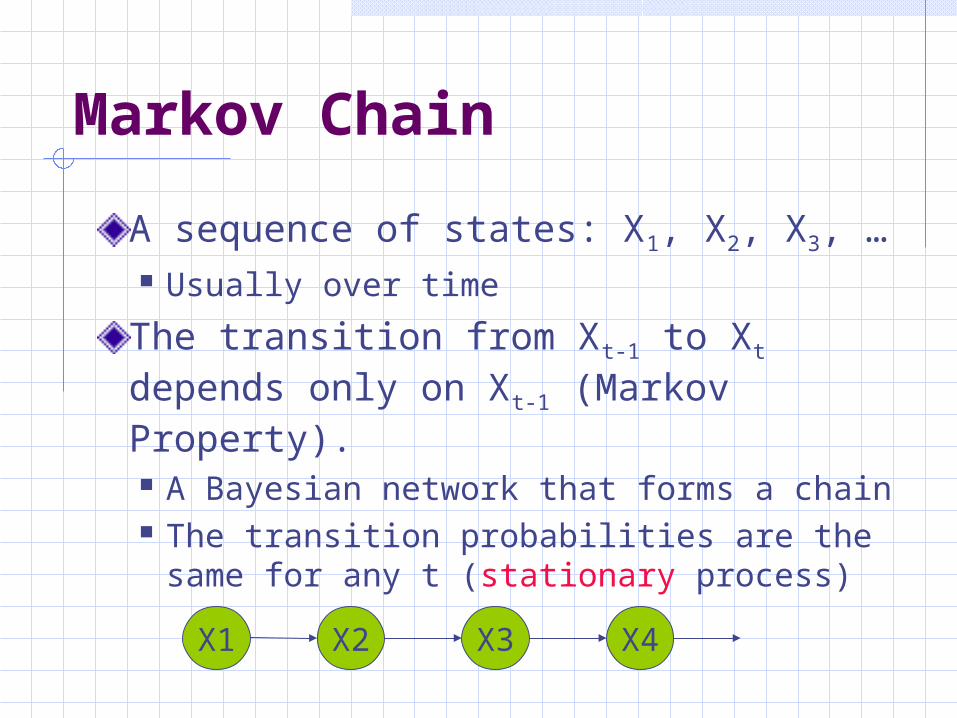
A sequence of states: X1, X2, X3, … Usually over time
The transition from Xt-1 to Xt depends only on Xt-1 (Markov Property). A Bayesian network that forms a chain The transition probabilities are the same
for any t (stationary process)
X2 X3 X4X1
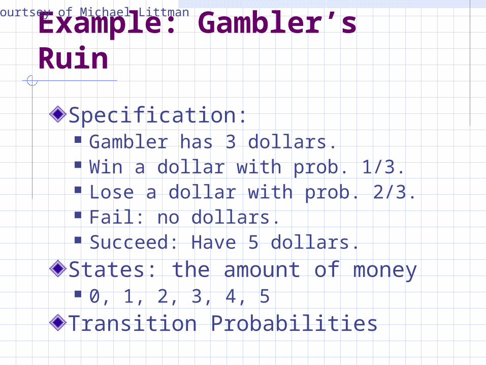
Example: Gambler’s Ruin
Specification: Gambler has 3 dollars. Win a dollar with prob. 1/3. Lose a dollar with prob. 2/3. Fail: no dollars. Succeed: Have 5 dollars.
States: the amount of money 0, 1, 2, 3, 4, 5
Transition Probabilities
Courtsey of Michael Littman

Example: Bi-gram Language Modeling
States:Transition Probabilities:
Transition Probabilities
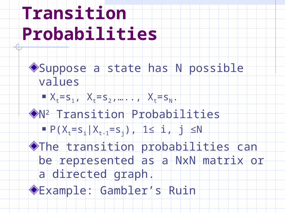
Suppose a state has N possible values Xt=s1, Xt=s2,….., Xt=sN.
N2 Transition Probabilities P(Xt=si|Xt-1=sj), 1≤ i, j ≤N
The transition probabilities can be represented as a NxN matrix or a directed graph.Example: Gambler’s Ruin
What can Markov Chains Do?
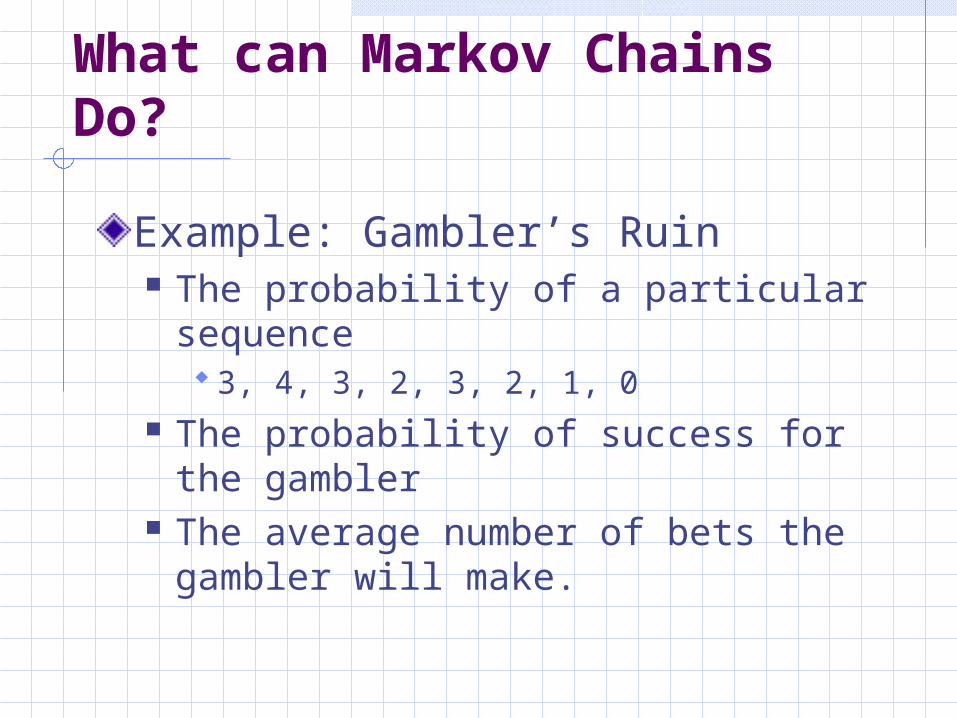
Example: Gambler’s Ruin The probability of a particular
sequence 3, 4, 3, 2, 3, 2, 1, 0
The probability of success for the gambler
The average number of bets the gambler will make.
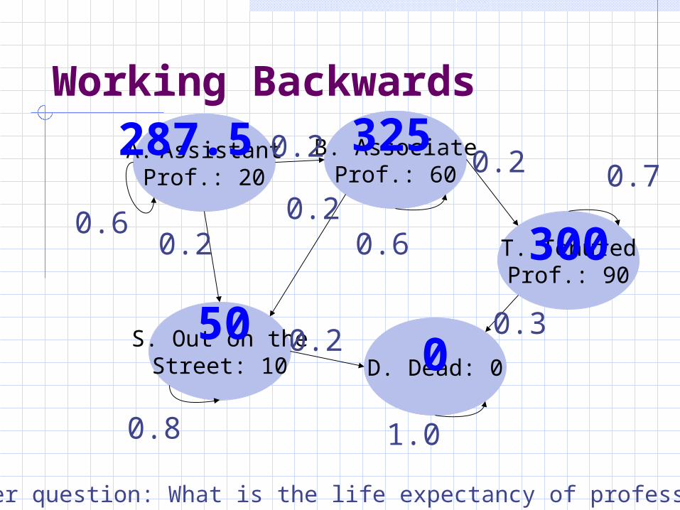
Working Backwards
A. AssistantProf.: 20
B. AssociateProf.: 60
T. TenuredProf.: 90
S. Out on theStreet: 10 D. Dead: 0
1.0
0.60.2
0.2
0.8
0.2
0.6
0.2
0.20.7
0.30
300
50
325287.5
Another question: What is the life expectancy of professors?
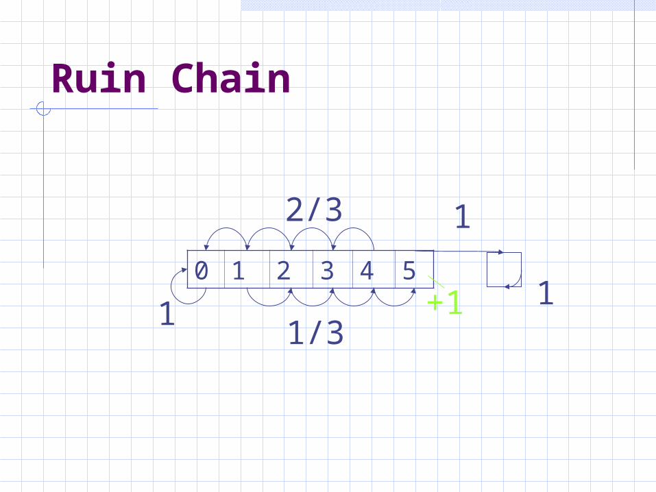
Ruin Chain
0 1 2 3 4 5
1/3
2/3
1
1
1+1
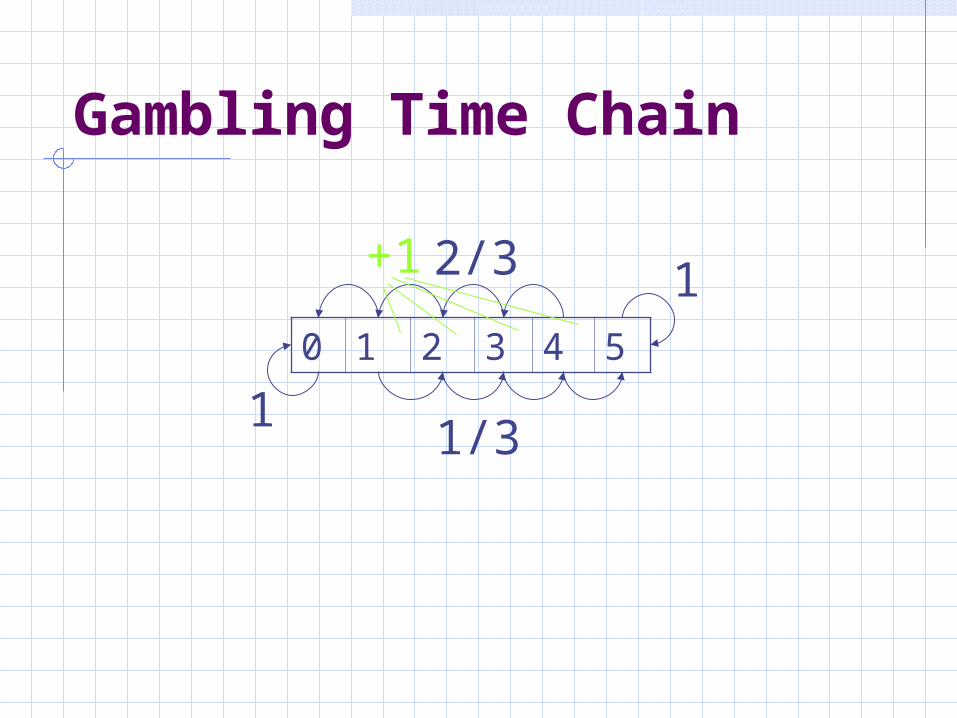
Gambling Time Chain
0 1 2 3 4 5
1/3
2/3 1
1
+1
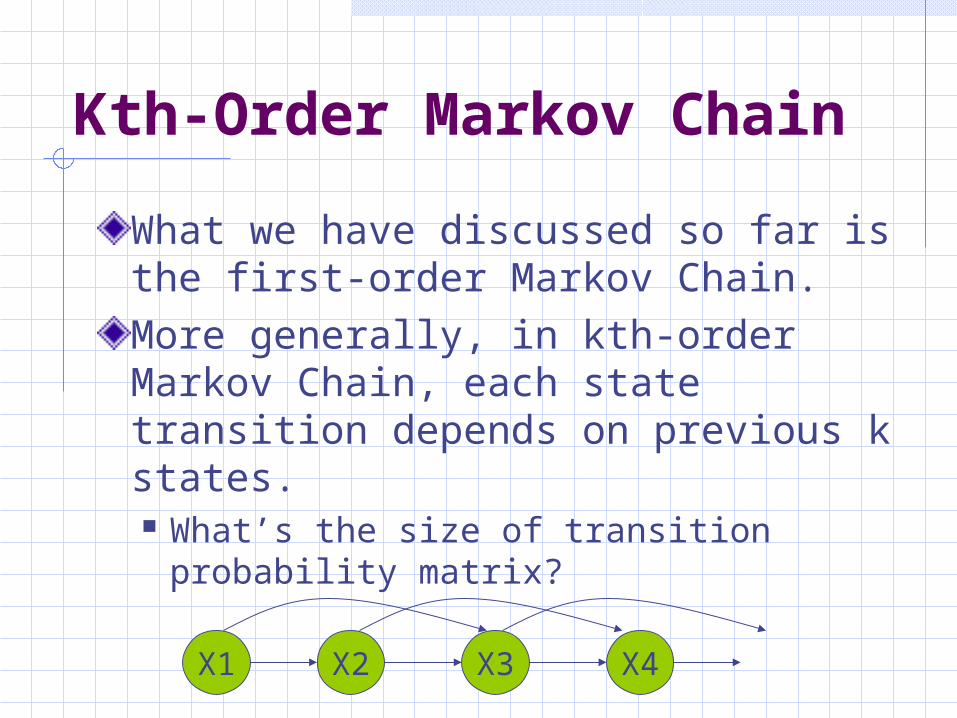
Kth-Order Markov Chain
What we have discussed so far is the first-order Markov Chain.More generally, in kth-order Markov Chain, each state transition depends on previous k states. What’s the size of transition
probability matrix?
X2 X3 X4X1
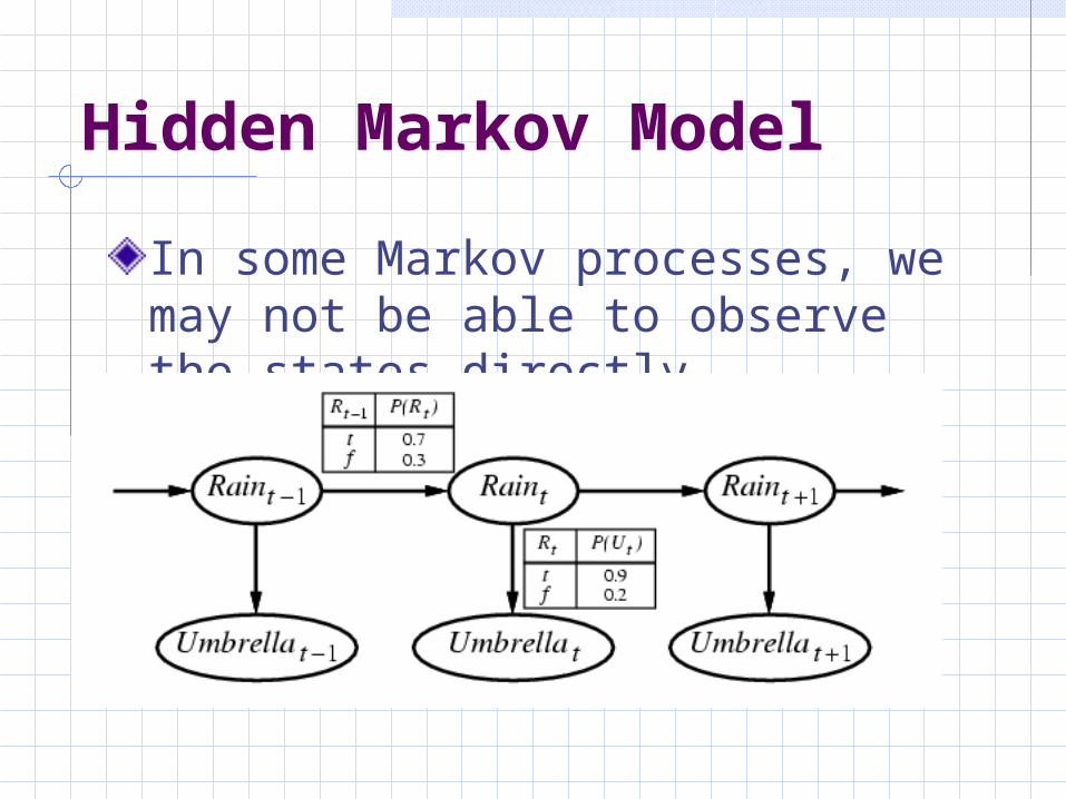
Hidden Markov Model
In some Markov processes, we may not be able to observe the states directly.
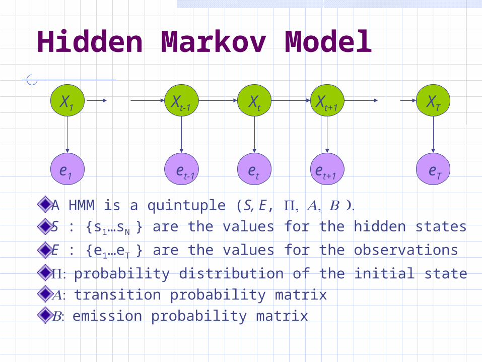
Hidden Markov Model
A HMM is a quintuple (S, E, S : {s1…sN } are the values for the hidden states
E : {e1…eT } are the values for the observations
probability distribution of the initial statetransition probability matrix emission probability matrix
Xt+1XtXt-1
et+1etet-1
X1
e1
XT
eT

Alternative Specification
If we define a special initial state, which does not emit anything, the probability distribution becomes part of transition probability matrix.
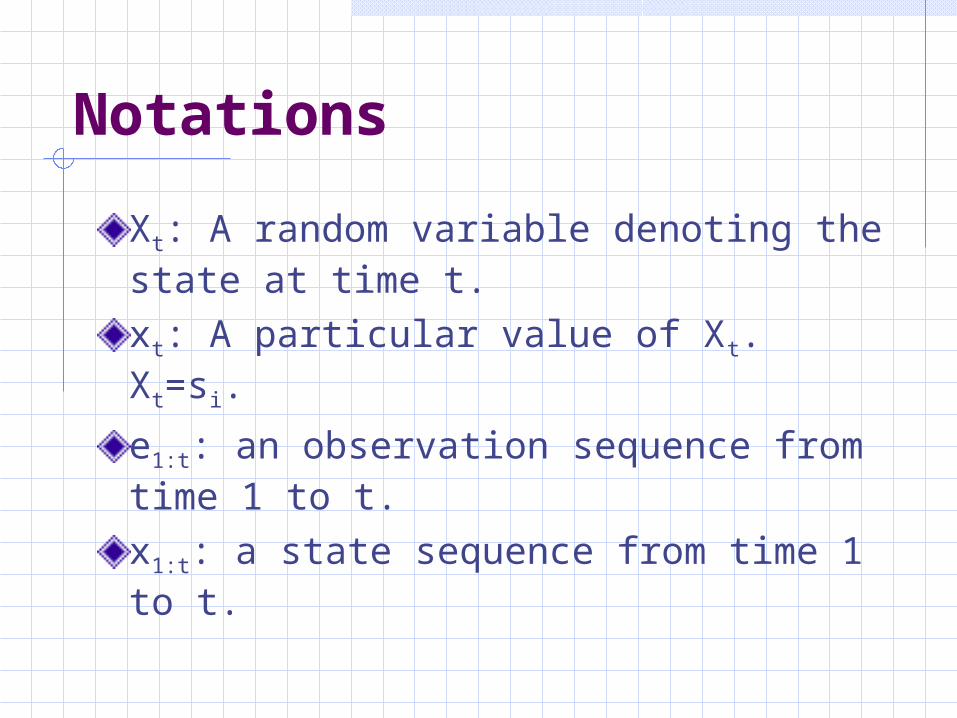
Notations
Xt: A random variable denoting the state at time t.xt: A particular value of Xt. Xt=si.
e1:t: an observation sequence from time 1 to t.x1:t: a state sequence from time 1 to t.
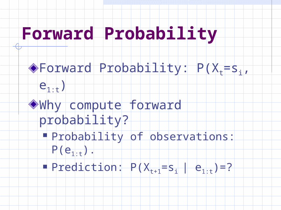
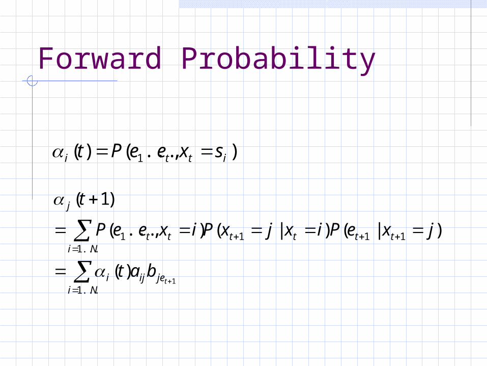
Forward Probability
Forward Probability: P(Xt=si, e1:t)
Why compute forward probability? Probability of observations: P(e1:t). Prediction: P(Xt+1=si | e1:t)=?
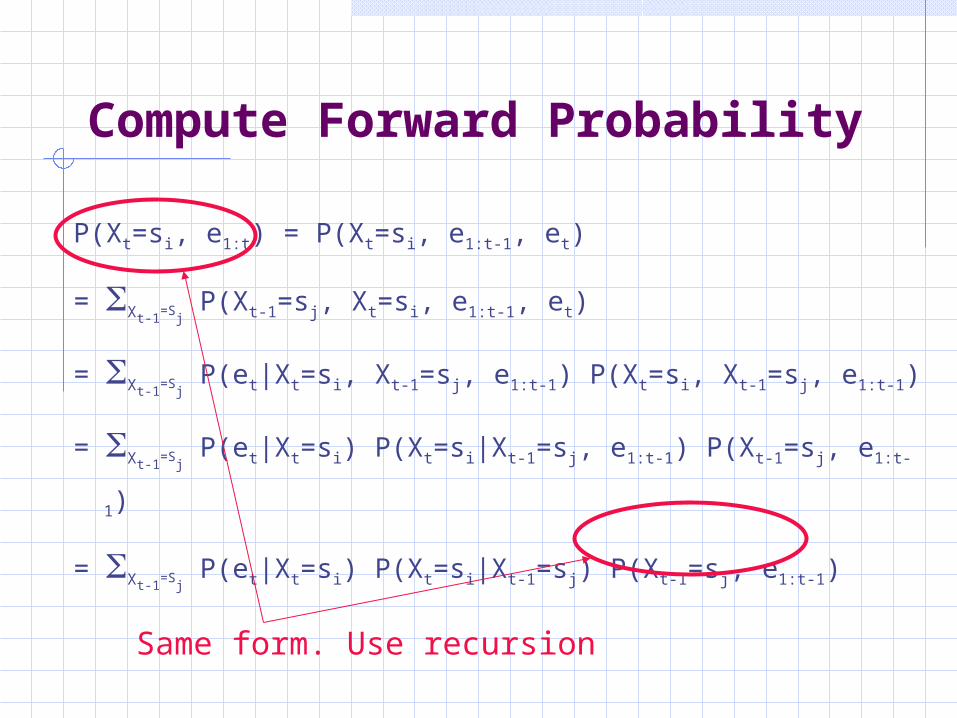
Compute Forward Probability
P(Xt=si, e1:t) = P(Xt=si, e1:t-1, et)
= Xt-1=S
j P(Xt-1=sj, Xt=si, e1:t-1, et)
= Xt-1=S
j P(et|Xt=si, Xt-1=sj, e1:t-1) P(Xt=si, Xt-1=sj, e1:t-1)
= Xt-1=S
j P(et|Xt=si) P(Xt=si|Xt-1=sj, e1:t-1) P(Xt-1=sj, e1:t-1)
= Xt-1=S
j P(et|Xt=si) P(Xt=si|Xt-1=sj) P(Xt-1=sj, e1:t-1)
Same form. Use recursion
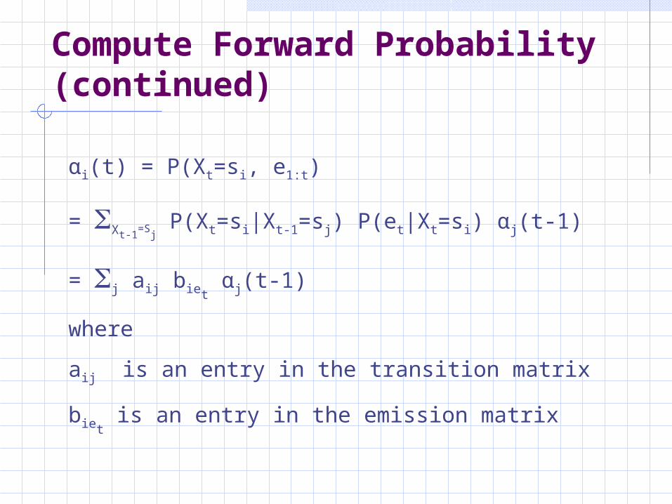
Compute Forward Probability (continued)
αi(t) = P(Xt=si, e1:t)
= Xt-1=S
j P(Xt=si|Xt-1=sj) P(et|Xt=si) αj(t-1)
= j aij biet αj(t-1)
where
aij is an entry in the transition matrix
biet is an entry in the emission matrix
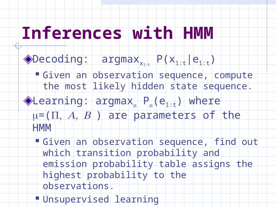
Inferences with HMM
Decoding: argmaxx1:t P(x1:t|e1:t)
Given an observation sequence, compute the most likely hidden state sequence.
Learning: argmax P(e1:t) where =() are parameters of the HMM Given an observation sequence, find out
which transition probability and emission probability table assigns the highest probability to the observations.
Unsupervised learning
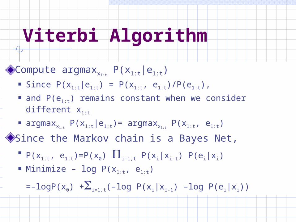
Viterbi Algorithm
Compute argmaxx1:t P(x1:t|e1:t)
Since P(x1:t|e1:t) = P(x1:t, e1:t)/P(e1:t), and P(e1:t) remains constant when we consider different x1:t
argmaxx1:t P(x1:t|e1:t)= argmaxx1:t
P(x1:t, e1:t)
Since the Markov chain is a Bayes Net, P(x1:t, e1:t)=P(x0) i=1,t P(xi|xi-1) P(ei|xi) Minimize – log P(x1:t, e1:t)
=–logP(x0) +i=1,t(–log P(xi|xi-1) –log P(ei|xi))
Viterbi Algorithm
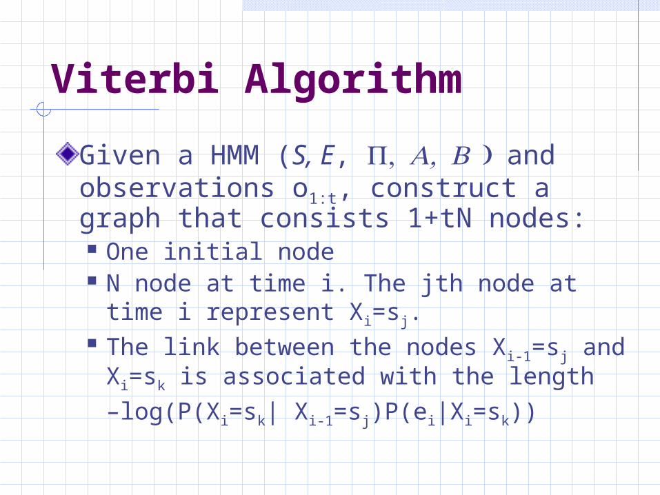
Given a HMM (S, E, and observations o1:t, construct a graph that consists 1+tN nodes: One initial node N node at time i. The jth node at time i
represent Xi=sj. The link between the nodes Xi-1=sj and
Xi=sk is associated with the length
–log(P(Xi=sk| Xi-1=sj)P(ei|Xi=sk))
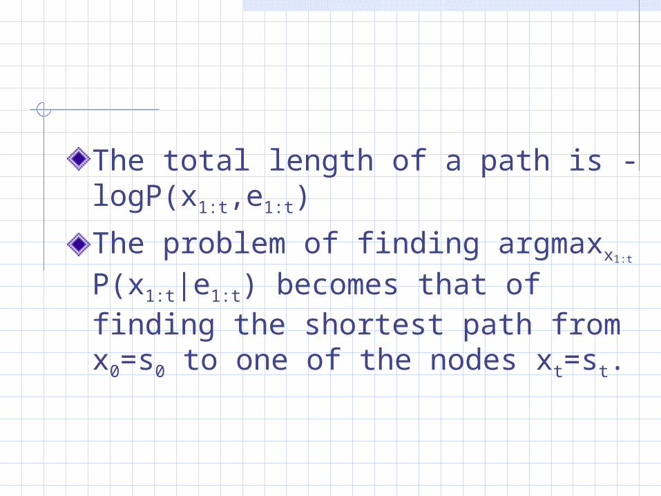
The total length of a path is -logP(x1:t,e1:t)
The problem of finding argmaxx1:t
P(x1:t|e1:t) becomes that of finding the shortest path from x0=s0 to one of the nodes xt=st.
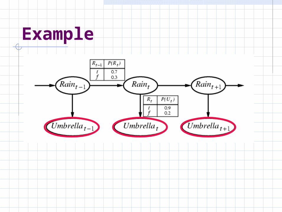
Example
Baum-Welch Algorithm
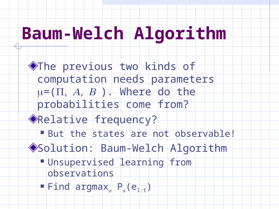
The previous two kinds of computation needs parameters =(). Where do the probabilities come from?Relative frequency? But the states are not observable!
Solution: Baum-Welch Algorithm Unsupervised learning from observations Find argmax P(e1:t)
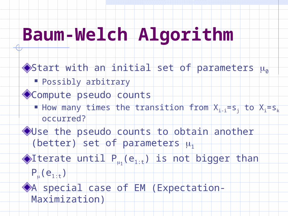
Baum-Welch Algorithm
Start with an initial set of parameters 0
Possibly arbitrary
Compute pseudo counts How many times the transition from Xi-i=sj to Xi=sk
occurred?
Use the pseudo counts to obtain another (better) set of parameters 1
Iterate until P1(e1:t) is not bigger than P(e1:t)
A special case of EM (Expectation-Maximization)
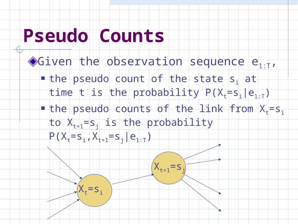
Pseudo CountsGiven the observation sequence e1:T, the pseudo count of the state si at time t is
the probability P(Xt=si|e1:T) the pseudo counts of the link from Xt=si to
Xt+1=sj is the probability P(Xt=si,Xt+1=sj|e1:T)
Xt=si
Xt+1=sj
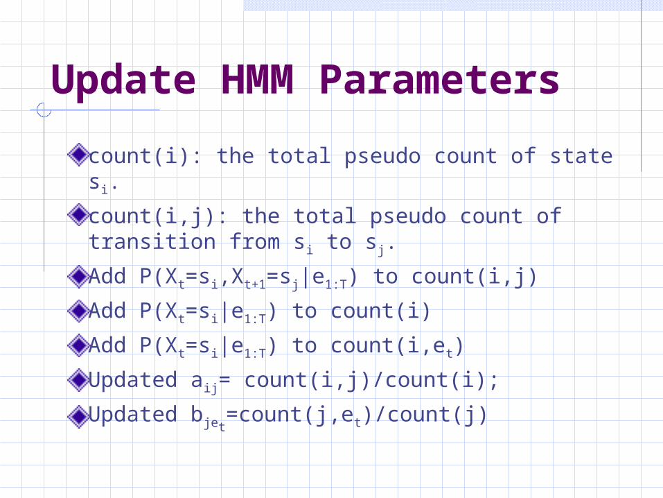
Update HMM Parameters
count(i): the total pseudo count of state si.
count(i,j): the total pseudo count of transition from si to sj.
Add P(Xt=si,Xt+1=sj|e1:T) to count(i,j)
Add P(Xt=si|e1:T) to count(i)
Add P(Xt=si|e1:T) to count(i,et)
Updated aij= count(i,j)/count(i);
Updated bjet=count(j,et)/count(j)
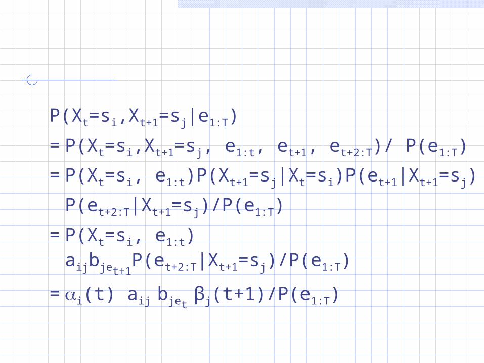
P(Xt=si,Xt+1=sj|e1:T)
=P(Xt=si,Xt+1=sj, e1:t, et+1, et+2:T)/ P(e1:T)
=P(Xt=si, e1:t)P(Xt+1=sj|Xt=si)P(et+1|Xt+1=sj)
P(et+2:T|Xt+1=sj)/P(e1:T)
=P(Xt=si, e1:t) aijbjet+1P(et+2:T|Xt+1=sj)/P(e1:T)
=i(t) aij bjet βj(t+1)/P(e1:T)
Forward Probability
),...()( 1 itti sxeePt
Nijeiji
ttttNi
tt
j
tbat
jxePixjxPixeeP
t
...1
111...1
1
1)(
)|()|(),...(
)1(
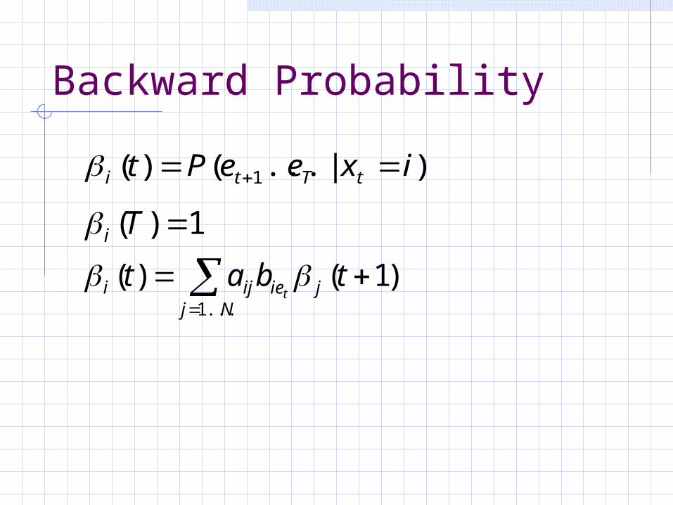
Backward Probability
)|...()( 1 ixeePt tTti
1)( Ti
Nj
jieiji tbatt
...1
)1()(
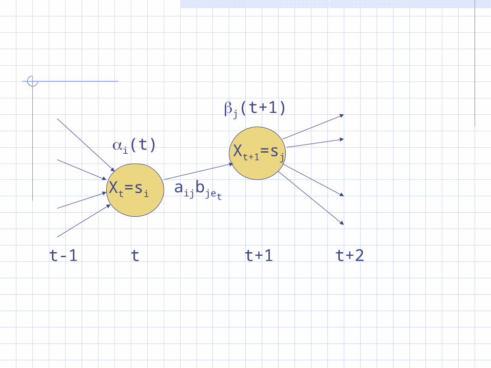
Xt=si
Xt+1=sj
t-1 t t+1 t+2
i(t)
j(t+1)
aijbjet
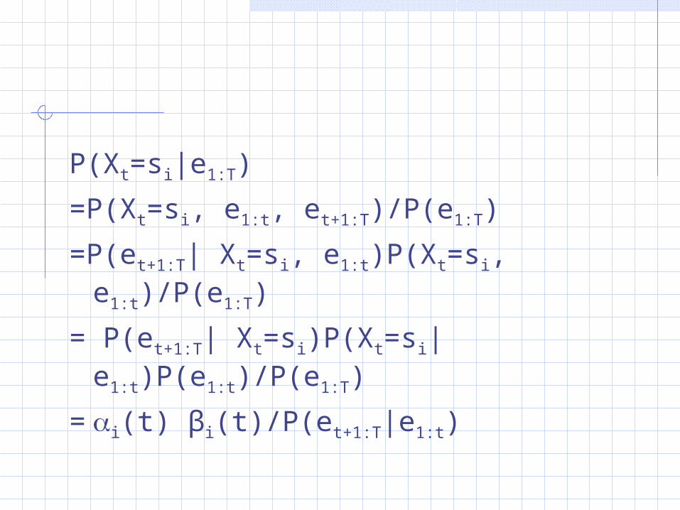
P(Xt=si|e1:T)
=P(Xt=si, e1:t, et+1:T)/P(e1:T)
=P(et+1:T| Xt=si, e1:t)P(Xt=si, e1:t)/P(e1:T)
= P(et+1:T| Xt=si)P(Xt=si|e1:t)P(e1:t)/P(e1:T)
=i(t) βi(t)/P(et+1:T|e1:t)


