Page 1
MIT 2.853/2.854
Introduction to Manufacturing Systems
Markov Processes and Queues
Stanley B. GershwinLaboratory for Manufacturing and Productivity
Massachusetts Institute of Technology
Markov Processes 1 Copyright ©c 2016 Stanley B. Gershwin.
Page 2
Stochastic processes
Stochastic processes
• t is time.
• X () is a stochastic process if X (t) is a randomvariable for every t.
• t is a scalar — it can be discrete or continuous.
• X (t) can be discrete or continuous, scalar orvector.
Markov Processes 2 Copyright ©c 2016 Stanley B. Gershwin.
Page 3
Stochastic processes Markov processes
Stochastic processesMarkov processes
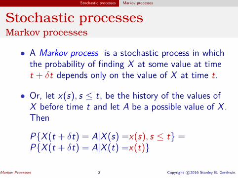
• A Markov process is a stochastic process in whichthe probability of finding X at some value at timet + δt depends only on the value of X at time t.
• Or, let x(s), s ≤ t, be the history of the values ofX before time t and let A be a possible value of X .Then
P{X (t + δt) = A|X (s) =x(s), s ≤ t} =P{X (t + δt) = A|X (t) =x(t)}
Markov Processes 3 Copyright ©c 2016 Stanley B. Gershwin.
Page 4
Stochastic processes Markov processes
Stochastic processesMarkov processes
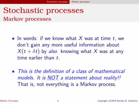
• In words: if we know what X was at time t, wedon’t gain any more useful information aboutX (t + δt) by also knowing what X was at anytime earlier than t.
• This is the definition of a class of mathematicalmodels. It is NOT a statement about reality!!That is, not everything is a Markov process.
Markov Processes 4 Copyright ©c 2016 Stanley B. Gershwin.
Page 5
Markov processes Example
Markov processesExample
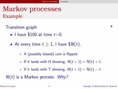
Transition graph *• I have $100 at time t=0.
• At every time t ≥ 1, I have $N(t).
? A (possibly biased) coin is flipped.
? If it lands with H showing, N(t + 1) = N(t) + 1.
? If it lands with T showing, N(t + 1) = N(t)− 1.
N(t) is a Markov process. Why?
Markov Processes 5 Copyright ©c 2016 Stanley B. Gershwin.
Page 6
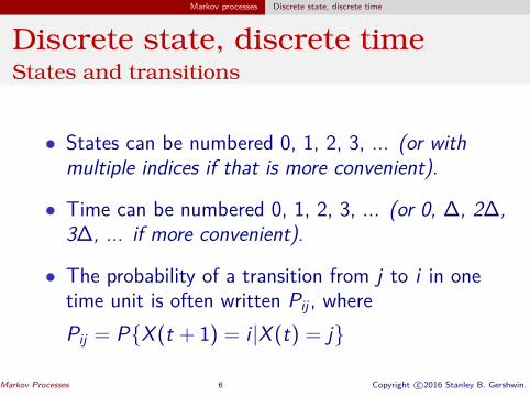
Markov processes Discrete state, discrete time
Discrete state, discrete timeStates and transitions
• States can be numbered 0, 1, 2, 3, ... (or withmultiple indices if that is more convenient).
• Time can be numbered 0, 1, 2, 3, ... (or 0, ∆, 2∆,3∆, ... if more convenient).
• The probability of a transition from j to i in onetime unit is often written Pij , wherePij = P{X (t + 1) = i |X (t) = j}
Markov Processes 6 Copyright ©c 2016 Stanley B. Gershwin.
Page 7
Markov processes Discrete state, discrete time
States and transitionsTransition graph
Transition graph P1414 1 −P − P −P
1414 24 64
P P24 64
P45
1
2
3
4
5
6
7
Pij is a probability. Note that Pii = 1−∑m,m=i Pmi . *6
Markov Processes 7 Copyright ©c 2016 Stanley B. Gershwin.
Page 8
Markov processes Discrete state, discrete time
States and transitionsTransition graph
Example : H(t) is the number of Hs after t coin flips.
Assume probability of H is p.
p p p p p
1−p 1−p 1−p 1−p 1−p
0 1 2 3 4
Markov Processes 8 Copyright ©c 2016 Stanley B. Gershwin.
Page 9
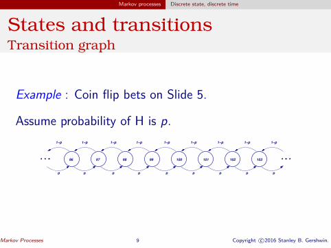
Markov processes Discrete state, discrete time
States and transitionsTransition graph
Example : Coin flip bets on Slide 5.
Assume probability of H is p.
p
1−p
p
1−p
p
1−p
p
1−p
p
1−p
p
1−p
p
1−p
p
1−p
p
1−p
100 1029896 10397 10199
Markov Processes 9 Copyright ©c 2016 Stanley B. Gershwin.
Page 10
Markov processes Discrete state, discrete time
Markov processesNotation
• {X (t) = i} is the event that random quantity X (t)has value i .
? Example: X (t) is any state in the graph on slide 7. iis a particular state.
• Define πi(t) = P{X (t) = i}.
• Normalization equation: ∑i πi(t) = 1.
Markov Processes 10 Copyright ©c 2016 Stanley B. Gershwin.
Page 11
Markov processes Discrete state, discrete time
Markov processesTransition equations
Transition equations: application of the law of total probability.
P45
14P14
P24
P64
1 − −−
4
5
π4(t + 1) = π5(t)P45
+ π4(t)(1− P14 − P24 − P64)
(Remember thatP45 = P{X (t + 1) = 4|X (t) = 5},P44 = P{X (t + 1) = 4|X (t) = 4}
(Detail of graph = 1− P14 − P24 − P64)on slide 7.)
Markov Processes 11 Copyright ©c 2016 Stanley B. Gershwin.
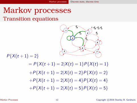
Page 12
Markov processes Discrete state, discrete time
Markov processesTransition equations
P1414 1 −P − P −P
1414 24 64
1
P P424 64
2 P45
6
5
3 7
P{X (t + 1) = 2}
= P{X (t + 1) = 2|X (t) = 1}P{X (t) = 1}
+P{X (t + 1) = 2|X (t) = 2}P{X (t) = 2}+P{X (t + 1) = 2|X (t) = 4}P{X (t) = 4}+P{X (t + 1) = 2|X (t) = 5}P{X (t) = 5}
Markov Processes 12 Copyright ©c 2016 Stanley B. Gershwin.
Page 13
Markov processes Discrete state, discrete time
Markov processesTransition equations
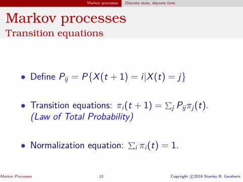
• Define Pij = P{X (t + 1) = i |X (t) = j}
• Transition equations: πi(t + 1) = ∑j Pijπj(t).
(Law of Total Probability)
• Normalization equation: ∑i πi(t) = 1.
Markov Processes 13 Copyright ©c 2016 Stanley B. Gershwin.
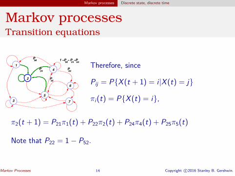
Page 14
Markov processes Discrete state, discrete time
Markov processesTransition equations
P1414 1 −P − P −P
1414 24 64
1
P P424 64
2 P45
6
5
3 7
Therefore, since
Pij = P{X (t + 1) = i |X (t) = j}
πi(t) = P{X (t) = i},
π2(t + 1) = P21π1(t) + P22π2(t) + P24π4(t) + P25π5(t)
Note that P22 = 1− P52.
Markov Processes 14 Copyright ©c 2016 Stanley B. Gershwin.
Page 15
Markov processes Discrete state, discrete time
Markov processesTransition equations — Matrix-Vector Form
For an n-state system, *
• Define π
P11 P 1(t)
12 ... P1n2()
1
)π(t = π t , P = P21 P22 ... P2n 1 , ν =
... ...
πn(t) Pn1 Pn2 ... Pnn
π π
...1
• Transition equations: (t + 1) = P (t)
• Normalization equation: Tν π(t) = 1
• Other facts:
T? ν P = Tν (Each column of P sums to 1.)? π(t) = P tπ(0)
Markov Processes 15 Copyright ©c 2016 Stanley B. Gershwin.
Page 16
Markov processes Discrete state, discrete time
Markov processesSteady state
• Steady state: πi = lim πi(t), if it exists.t→∞
• Steady-state transition equations: πi = ∑j Pijπj .
• Alternatively, steady-state balance equations:πi∑
m,m 6=i Pmi = ∑j ,j 6=i Pijπj
• Normalization equation: ∑i πi = 1.
Markov Processes 16 Copyright ©c 2016 Stanley B. Gershwin.
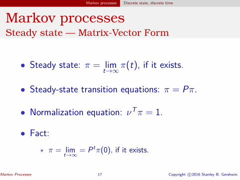
Page 17
Markov processes Discrete state, discrete time
Markov processesSteady state — Matrix-Vector Form
• Steady state: π = lim π(t), if it exists.t→∞
• Steady-state transition equations: π = Pπ.
• Normalization equation: Tν π = 1.
• Fact:? π = lim = P tπ(0), if it exists.
t→∞
Markov Processes 17 Copyright ©c 2016 Stanley B. Gershwin.
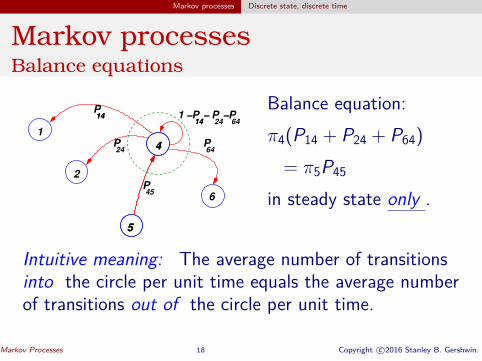
Page 18
Markov processes Discrete state, discrete time
Markov processesBalance equations
P1414 1 −P − P −P
1414 24 64
1
P P4424 64
2
P45
6
55
Balance equation:π4(P14 + P24 + P64)
= π5P45
in steady state only .
Intuitive meaning: The average number of transitionsinto the circle per unit time equals the average numberof transitions out of the circle per unit time.
Markov Processes 18 Copyright ©c 2016 Stanley B. Gershwin.
Page 19
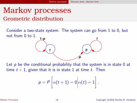
Markov processes Discrete state, discrete time
Markov processesGeometric distribution
Consider a two-state system. The system can go from 1 to 0, butnot from 0 to 1.
1 0
p
1−p 1
Let p be the conditional probability that the system is in state 0 attime t + 1, given that it is in state 1 at time t. Then
p = P[α(t + 1) = 0
∣∣∣∣∣α(t) = 1].
Markov Processes 19 Copyright ©c 2016 Stanley B. Gershwin.
Page 20
Markov processes Discrete state, discrete time
Markov processesGeometric distribution — Transition equations
Let π(α, t) be the probability of being in state α at time t. Then, since
π(0, t + 1) = P[α(t + 1) = 0
∣∣∣∣α(t) = 1]
P[α(t) = 1]
+P[α(t + 1) = 0
∣∣α(t) = 0
]w
∣∣ P[α(t) = 0],
e have
π(0, t + 1) = pπ(1, t) + π(0, t),π(1, t + 1) = (1− p)π(1, t),
and the normalization equation
π(1, t) + π(0, t) = 1.
Markov Processes 20 Copyright ©c 2016 Stanley B. Gershwin.
Page 21
Markov processes Discrete state, discrete time
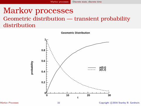
Markov processesGeometric distribution — transient probabilitydistribution
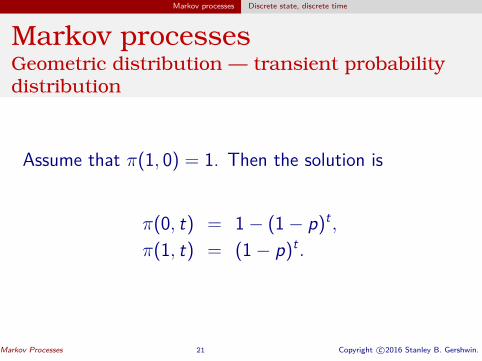
Assume that π(1, 0) = 1. Then the solution is
π(0, t) = 1− (1 t− p) ,π(1, t) = (1− p)t .
Markov Processes 21 Copyright ©c 2016 Stanley B. Gershwin.
Page 22
Markov processes Discrete state, discrete time
Markov processesGeometric distribution — transient probabilitydistribution
Geometric Distributionp
rob
abili
ty
t0 10 20 30
0
0.2
0.4
0.6
0.8
1
p(0,t)p(1,t)
Markov Processes 22 Copyright ©c 2016 Stanley B. Gershwin.
Page 23
Markov processes Discrete state, discrete time
Markov processesUnreliable machine
1=up; 0=down.
p
1 0
1−p 1−rr
Markov Processes 23 Copyright ©c 2016 Stanley B. Gershwin.
Page 24
Markov processes Discrete state, discrete time
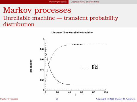
Markov processesUnreliable machine — transient probabilitydistribution
The probability distribution satisfies
π(0, t + 1) = π(0, t)(1− r) + π(1, t)p,
π(1, t + 1) = π(0, t)r + π(1, t)(1− p).
Markov Processes 24 Copyright ©c 2016 Stanley B. Gershwin.
Page 25
Markov processes Discrete state, discrete time
Markov processesUnreliable machine — transient probabilitydistribution
It is not hard to show that
tπ(0, t) = π(0, 0)(1− p − r)p+ [1r + p − (1− p − r)t ] ,
π(1 t, t) = π(1, 0)(1− p − r)r+ [1r + p − (1− p − r)t ] .
Markov Processes 25 Copyright ©c 2016 Stanley B. Gershwin.
Page 26
Markov processes Discrete state, discrete time
Markov processesUnreliable machine — transient probabilitydistribution
Discrete Time Unreliable Machinep
rob
abili
ty
t0 20 40 60 80 100
0
0.2
0.4
0.6
0.8
1
p(0,t)p(1,t)
Markov Processes 26 Copyright ©c 2016 Stanley B. Gershwin.
Page 27
Markov processes Discrete state, discrete time
Markov processesUnreliable machine — steady-state probabilitydistribution
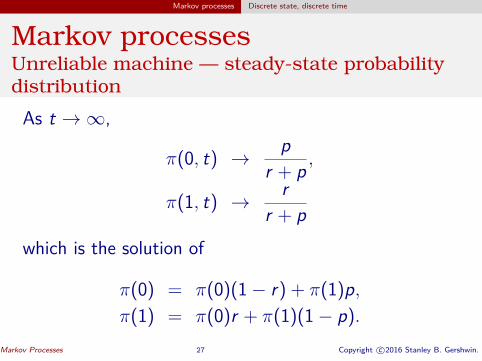
As t →∞,p
π(0, t) → r + p ,r
π(1, t) → r + p
which is the solution of
π(0) = π(0)(1− r) + π(1)p,π(1) = π(0)r + π(1)(1− p).
Markov Processes 27 Copyright ©c 2016 Stanley B. Gershwin.
Page 28
Markov processes Discrete state, discrete time
Markov processesUnreliable machine — efficiency
If a machine makes one part per time unit when it is operational,its average production rate is
rπ(1) = r + p
This quantity is the efficiency of the machine.
If the machine makes one part per τ time units when it isoperational, its average production rate is
1P = rτ
(r + p
)
Markov Processes 28 Copyright ©c 2016 Stanley B. Gershwin.
Page 29
Markov processes Discrete state, continuous time
Discrete state, continuous timeStates and transitions
• States can be numbered 0, 1, 2, 3, ... (or withmultiple indices if that is more convenient).
• Time is a real number, defined on (−∞,∞) or asmaller interval.
• The probability of a transition from j to i during[t, t + δt] is approximately λijδt, where δt is small,andλijδt ≈ P{X (t + δt) = i |X (t) = j} for i 6= j
Markov Processes 29 Copyright ©c 2016 Stanley B. Gershwin.
Page 30
Markov processes Discrete state, continuous time
Discrete state, continuous timeStates and transitions
More precisely,
λijδt = P{X (t + δt) = i |X (t) = j}+ o(δt)for i 6= j
o(δt)where o(δt) is a function that satisfies limδt→0
= 0δt
This implies that for small δt, o(δt)� δt.
Markov Processes 30 Copyright ©c 2016 Stanley B. Gershwin.
Page 31
Markov processes Discrete state, continuous time
Discrete state, continuous timeStates and transitions
Transition graph1
2
3
4
5
6
7
1414
λ24
λ45
λ64
λ
λij is a probability rate. λijδt is a probability.
Compare with the discrete-time graph.
Markov Processes 31 Copyright ©c 2016 Stanley B. Gershwin.
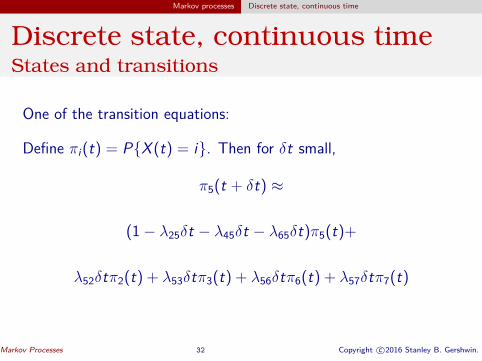
Page 32
Markov processes Discrete state, continuous time
Discrete state, continuous timeStates and transitions
One of the transition equations:
Define πi(t) = P{X (t) = i}. Then for δt small,
π5(t + δt) ≈
(1− λ25δt − λ45δt − λ65δt)π5(t)+
λ52δtπ2(t) + λ53δtπ3(t) + λ56δtπ6(t) + λ57δtπ7(t)
Markov Processes 32 Copyright ©c 2016 Stanley B. Gershwin.
Page 33
Markov processes Discrete state, continuous time
Discrete state, continuous timeStates and transitions
Or,
π5(t + δt) ≈
π5(t)− (λ25 + λ45 + λ65)π5(t)δt
+(λ52π2(t) + λ53π3(t) + λ56π6(t) + λ57π7(t))δt
Markov Processes 33 Copyright ©c 2016 Stanley B. Gershwin.
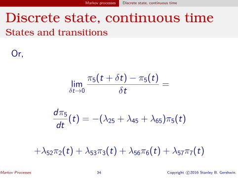
Page 34
Markov processes Discrete state, continuous time
Discrete state, continuous timeStates and transitions
Or,
lim π5(t + δt)− π5(t)δt→0
=δt
dπ5 (t) =dt −(λ25 + λ45 + λ65)π5(t)
+λ52π2(t) + λ53π3(t) + λ56π6(t) + λ57π7(t)
Markov Processes 34 Copyright ©c 2016 Stanley B. Gershwin.
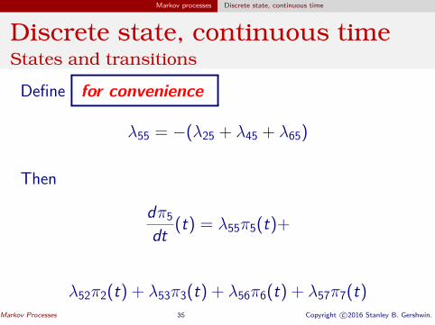
Page 35
Markov processes Discrete state, continuous time
Discrete state, continuous timeStates and transitions
Define for convenience
λ55 = −(λ25 + λ45 + λ65)
Then
dπ5 (t) =dt λ55π5(t)+
λ52π2(t) + λ53π3(t) + λ56π6(t) + λ57π7(t)Markov Processes 35 Copyright ©c 2016 Stanley B. Gershwin.
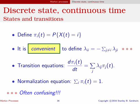
Page 36
Markov processes Discrete state, continuous time
Discrete state, continuous timeStates and transitions
• Define πi(t) = P{X (t) = i}
• It is convenient to define λii = −∑j 6=i λji ∗ ∗ ∗
d• Transition equations: πi(t) =dt∑λijπj(t).
j
• Normalization equation: ∑i πi(t) = 1.
∗ ∗ ∗ Often confusing!!!Markov Processes 36 Copyright ©c 2016 Stanley B. Gershwin.
Page 37
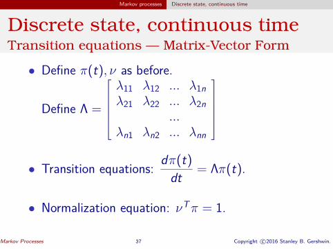
Markov processes Discrete state, continuous time
Discrete state, continuous timeTransition equations — Matrix-Vector Form
• Define π(t), asν before.λ11 λ12 ... λ1n
Define Λ =
λ21 λ22 ... λ2n ...
λn1 λn2 ... λnn
d )Transition equations: π(t• = Λdt π(t).
• Normalization equation: Tν π = 1.
Markov Processes 37 Copyright ©c 2016 Stanley B. Gershwin.
Page 38
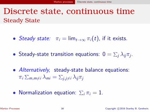
Markov processes Discrete state, continuous time
Discrete state, continuous timeSteady State
• Steady state: πi = limt πi(t), if it exists.→∞
• Steady-state transition equations: 0 = ∑j λijπj .
• Alternatively, steady-state balance equations:πi∑
m,m 6=i λmi = ∑j ,j 6=i λijπj
• Normalization equation: ∑i πi = 1.
Markov Processes 38 Copyright ©c 2016 Stanley B. Gershwin.
Page 39
Markov processes Discrete state, continuous time
Discrete state, continuous timeSteady State — Matrix-Vector Form
• Steady state: π = lim π(t), if it exists.t→∞
• Steady-state transition equations: 0 = Λπ.
• Normalization equation: Tν π = 1.
Markov Processes 39 Copyright ©c 2016 Stanley B. Gershwin.
Page 40
Markov processes Discrete state, continuous time
Discrete state, continuous timeSources of confusion in continuous time models
• Never Draw self-loops in continuous timemarkov process graphs.
• Never write 1− λ14 − λ24 − λ64. Write? 1− (λ14 + λ24 + λ64)δt, or? −(λ14 + λ24 + λ64)
• λii = −∑j 6=i λji is NOT a rate and NOT a
probability. It is ONLY a convenient notation.
Markov Processes 40 Copyright ©c 2016 Stanley B. Gershwin.
Page 41
Markov processes Discrete state, continuous time
Discrete state, continuous timeExponential distribution
Exponential random variable T : the time to move fromstate 1 to state 0.
1 0
µ
Markov Processes 41 Copyright ©c 2016 Stanley B. Gershwin.
Page 42
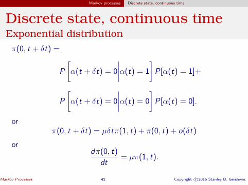
Markov processes Discrete state, continuous time
Discrete state, continuous timeExponential distributionπ(0, t + δt) =
P[α(t + δt) = 0
∣∣∣ ]∣∣α(t) = 1 P[α(t) = 1]+
P[α(t + δt) = 0
∣∣ ]∣∣∣α(t) = 0 P[α(t) = 0].
orπ(0, t + δt) = µδtπ(1, t) + π(0, t) + o(δt)
ordπ(0, t) =dt µπ(1, t).
Markov Processes 42 Copyright ©c 2016 Stanley B. Gershwin.
Page 43
Markov processes Discrete state, continuous time
Discrete state, continuous timeExponential distribution
Or,
dπ(1, t) = −µπ(1, t)dt .
If π(1, 0) = 1, then
π(1, t) = e−µt
andπ(0 t, t) = 1− e−µ
Markov Processes 43 Copyright ©c 2016 Stanley B. Gershwin.
Page 44
Markov processes Discrete state, continuous time
Discrete state, continuous timeExponential distribution
The probability that the transition takes place at some T ∈ [t, t + δt] is
P [α(t + δt) = 0 and α(t) = 1]
= P[α(t + δt) = 0|α(t) = 1]P[α(t) = 1]
= (µδt)(e−µt)
The exponential density function is therefore µe−µt for t ≥ 0 and 0 for t < 0.
The time of the transition from 1 to 0 is said to be exponentially distributedwith rate µ.
The expected transition time is 1/µ. (Prove it!)
Markov Processes 44 Copyright ©c 2016 Stanley B. Gershwin.
Page 45
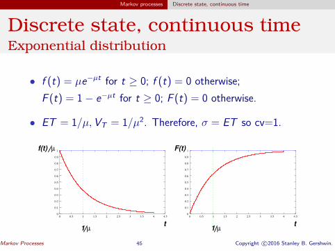
Markov processes Discrete state, continuous time
Discrete state, continuous timeExponential distribution
• f (t) = µe−µt for t ≥ 0; f (t) = 0 otherwise;F (t) = 1− e−µt for t ≥ 0; F (t) = 0 otherwise.
• ET = 1/µ,VT = 1 2/µ . Therefore, σ = ET so cv=1.
µ
µf(t)
t1 µ
F(t)
t1
0
0.1
0.2
0.3
0.4
0.5
0.6
0.7
0.8
0.9
1
0 0.5 2 2.5 3 3.5 4 4.51 1.50
0.1
0.2
0.3
0.4
0.5
0.6
0.7
0.8
0.9
1
0 0.5 2 2.5 3 3.5 4 4.51 1.5
Markov Processes 45 Copyright ©c 2016 Stanley B. Gershwin.
Page 46
Markov processes Discrete state, continuous time
Markov processesExponential
Density function
Exponential densityfunction and a smallnumber of samples.
Markov Processes 46 Copyright ©c 2016 Stanley B. Gershwin.
Page 47
Markov processes Discrete state, continuous time
Discrete state, continuous timeExponential distribution: some properties
• Memorylessness:P(T > t + x |T > x) = P(T > t)
• P(t ≤ T ≤ t + δt|T ≥ t) ≈ µδt for small δt.
Markov Processes 47 Copyright ©c 2016 Stanley B. Gershwin.
Page 48
Markov processes Discrete state, continuous time
Discrete state, continuous timeExponential distribution: some properties
• If T1, ...,Tn are independent exponentiallydistributed random variables with parametersµ1..., µn, and
• T = min(T1, ...,Tn), then
• T is an exponentially distributed random variablewith parameter µ = µ1 + ... + µn.
Markov Processes 48 Copyright ©c 2016 Stanley B. Gershwin.
Page 49
Markov processes Discrete state, continuous time
Discrete state, continuous timeUnreliable machine
Continuous time unreliable machine.r
up down
p
Markov Processes 49 Copyright ©c 2016 Stanley B. Gershwin.
Page 50
Markov processes Discrete state, continuous time
Discrete state, continuous timeUnreliable machine
From the Law of Total Probability:
P({the machine is up at time t + δt})=
P({the machine is up at time t + δt | the machine was up at time t}) ×P({the machine was up at time t}) +
P({the machine is up at time t + δt | the machine was down at time t}) ×P({the machine was down at time t})
+o(δt)
and similarly for P({the machine is down at time t + δt}).
Markov Processes 50 Copyright ©c 2016 Stanley B. Gershwin.
Page 51
Markov processes Discrete state, continuous time
Discrete state, continuous timeUnreliable machine
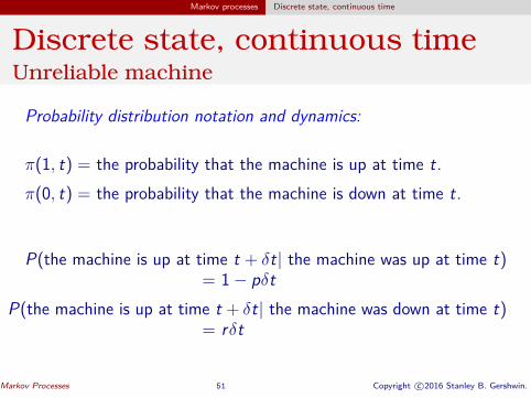
Probability distribution notation and dynamics:
π(1, t) = the probability that the machine is up at time t.π(0, t) = the probability that the machine is down at time t.
P(the machine is up at time t + δt| the machine was up at time t)= 1− pδt
P(the machine is up at time t + δt| the machine was down at time t)= rδt
Markov Processes 51 Copyright ©c 2016 Stanley B. Gershwin.
Page 52
Markov processes Discrete state, continuous time
Discrete state, continuous timeUnreliable machine
Therefore
π(1, t + δt) = (1− pδt)π(1, t) + rδtπ(0, t) + o(δt)
Similarly,
π(0, t + δt) = pδtπ(1, t) + (1− rδt)π(0, t) + o(δt)
Markov Processes 52 Copyright ©c 2016 Stanley B. Gershwin.
Page 53
Markov processes Discrete state, continuous time
Discrete state, continuous timeUnreliable machine
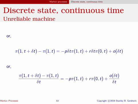
or,
π(1, t + δt)− π(1, t) = −pδtπ(1, t) + rδtπ(0, t) + o(δt)
or,
π(1, t + δt)− π(1, t) o(=δt −pπ(1, t) + rπ(0, t) + δt)
δt
Markov Processes 53 Copyright ©c 2016 Stanley B. Gershwin.
Page 54
Markov processes Discrete state, continuous time
Discrete state, continuous time
or,
dπ(0, t) =dt −π(0, t)r + π(1, t)p
dπ(1, t) =dt π(0, t)r − π(1, t)p
Markov Processes 54 Copyright ©c 2016 Stanley B. Gershwin.
Page 55
Markov processes Discrete state, continuous time
Markov processesUnreliable machine
Solution
pπ(0, t) = p+r + p
[π(0, 0)− er + p
]−(r+p)t
π(1, t) = 1− π(0, t).
As t →∞,p
π(0) → r + p ,r
π(1) → r + p
Markov Processes 55 Copyright ©c 2016 Stanley B. Gershwin.
Page 56
Markov processes Discrete state, continuous time
Markov processesUnreliable machine
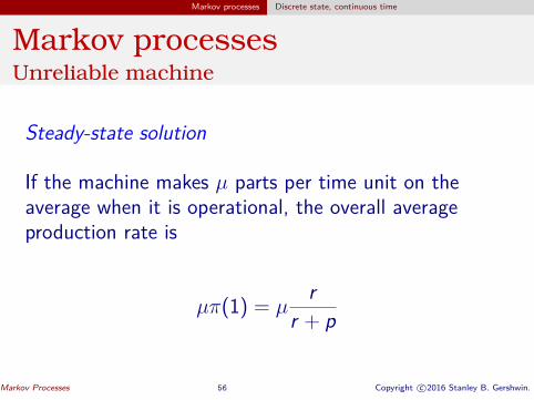
Steady-state solution
If the machine makes µ parts per time unit on theaverage when it is operational, the overall averageproduction rate is
rµπ(1) = µr + p
Markov Processes 56 Copyright ©c 2016 Stanley B. Gershwin.
Page 57
Markov processes Discrete state, continuous time
Discrete state, continuous timePoisson Process
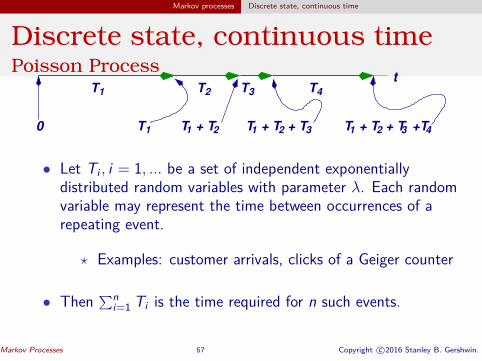
T1
T1 T2 T3 T4
T + T T + T + T T + T + T +T1 2 1 2 3 1 2 3 4
t
0
• Let Ti , i = 1, ... be a set of independent exponentiallydistributed random variables with parameter λ. Each randomvariable may represent the time between occurrences of arepeating event.
? Examples: customer arrivals, clicks of a Geiger counter
• Then ∑ni=1 Ti is the time required for n such events.
Markov Processes 57 Copyright ©c 2016 Stanley B. Gershwin.
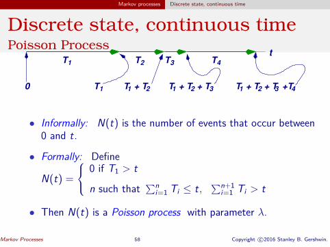
Page 58
Markov processes Discrete state, continuous time
Discrete state, continuous timePoisson Process
T1
T1 T2 T3 T4
T + T T + T + T T + T + T +T1 2 1 2 3 1 2 3 4
t
0
• Informally: N(t) is the number of events that occur between0 and t.
• Formally: Define
N(t) =
0 if T1 > t n such that ∑n n+1i=1 Ti ≤ t, i=1 Ti > t
• Then N(t) is a Poisson process with pa
∑rameter λ.
Markov Processes 58 Copyright ©c 2016 Stanley B. Gershwin.
Page 59
Markov processes Discrete state, continuous time
Discrete state, continuous timePoisson Process
P(N(t) = n) = e−λt (λt)n
n!
0.00
0.02
0.04
0.06
0.08
0.10
0.12
0.14
0.16
0.18
10987654321
n
Poisson Distribution
λt = 6Markov Processes 59 Copyright ©c 2016 Stanley B. Gershwin.
Page 60
Markov processes Discrete state, continuous time
Discrete state, continuous timePoisson Process
P(N(t) = n) = e−λt (λt)n
n! , λ = 2
n=1
n=2
n=3
n=4
n=5
n=10
t
P(N(t)=n)
0
0.05
0.1
0.15
0.2
0.25
0.3
0.35
0.4
0 2 3 4 5 6 7 8 1
Markov Processes 60 Copyright ©c 2016 Stanley B. Gershwin.
Page 61
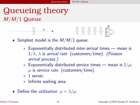
Queueing theory M/M/1 Queue
Queueing theoryM/M/1 Queue
λ
µ
• Simplest model is the M/M/1 queue:
? Exponentially distributed inter-arrival times — mean is1/λ; λ is arrival rate (customers/time). (Poissonarrival process.)
? Exponentially distributed service times — mean is 1/µ;µ is service rate (customers/time).
? 1 server.? Infinite waiting area.
• Define the utilization ρ = λ/µ.
Markov Processes 61 Copyright ©c 2016 Stanley B. Gershwin.
Page 62
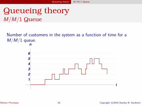
Queueing theory M/M/1 Queue
Queueing theoryM/M/1 Queue
Number of customers in the system as a function of time for aM/M/1 queue.
1
2
3
4
5
6
t
n
Markov Processes 62 Copyright ©c 2016 Stanley B. Gershwin.
Page 63
Queueing theory M/M/1 Queue
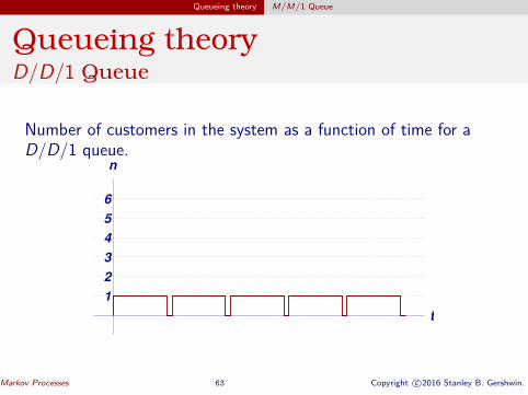
Queueing theoryD/D/1 Queue
Number of customers in the system as a function of time for aD/D/1 queue.
1
2
3
4
5
6
t
n
Markov Processes 63 Copyright ©c 2016 Stanley B. Gershwin.
Page 64
Queueing theory M/M/1 Queue
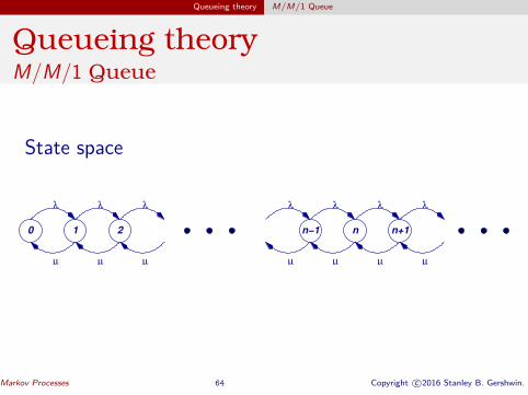
Queueing theoryM/M/1 Queue
State space
µ
λ
µ
λ
µ
λ
µ
λ
µ
λ
µ
λ
0 1 2
µ
λ
n−1 n n+1
Markov Processes 64 Copyright ©c 2016 Stanley B. Gershwin.
Page 65
Queueing theory M/M/1 Queue
Queueing theoryM/M/1 Queue
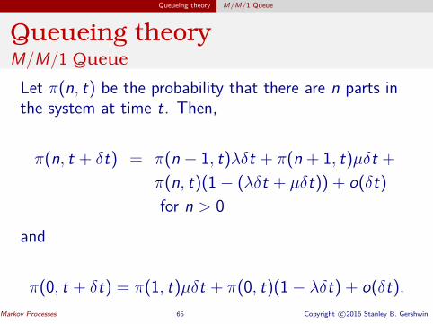
Let π(n, t) be the probability that there are n parts inthe system at time t. Then,
π(n, t + δt) = π(n − 1, t)λδt + π(n + 1, t)µδt +π(n, t)(1− (λδt + µδt)) + o(δt)for n > 0
and
π(0, t + δt) = π(1, t)µδt + π(0, t)(1− λδt) + o(δt).Markov Processes 65 Copyright ©c 2016 Stanley B. Gershwin.
Page 66
Queueing theory M/M/1 Queue
Queueing theoryM/M/1 Queue
Or,
dπ(n, t) =dt π(n − 1, t)λ + π(n + 1, t)µ− π(n, t)(λ + µ),n > 0
dπ(0, t) = π(1, t)µ− π(0dt , t)λ.
If a steady state distribution exists, it satisfies
0 = π(n − 1)λ + π(n + 1)µ− π(n)(λ + µ), n > 00 = π(1)µ− π(0)λ.
Why “if”?Markov Processes 66 Copyright ©c 2016 Stanley B. Gershwin.
Page 67
Queueing theory M/M/1 Queue
Queueing theoryM/M/1 Queue – Steady State
Let ρ = λ/µ. These equations are satisfied by
(n) = (1 ) nπ − ρ ρ , n ≥ 0if ρ < 1.
The average number of parts in the system is
n̄ =∑
nπ(n) = ρ
n 1− ρ = λ.
µ− λ
*Markov Processes 67 Copyright ©c 2016 Stanley B. Gershwin.
Page 68
Queueing theory Little’s Law
Queueing theoryLittle’s Law
• True for most systems of practical interest (not just M/M/1).
• Steady state only.
• L = the average number of customers in a system.
• W = the average delay experienced by a customer in thesystem.
L = λWIn the M/M/1 queue, L = n̄ and
1W = .µ− λ
Markov Processes 68 Copyright ©c 2016 Stanley B. Gershwin.
Page 69
Queueing theory M/M/1
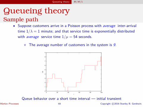
Queueing theorySample path
• Suppose customers arrive in a Poisson process with average inter-arrivaltime 1/λ = 1 minute; and that service time is exponentially distributedwith average service time 1/µ = 54 seconds.
? The average number of customers in the system is 9.
0
1
2
3
4
5
6
7
8
9
0 20 40 60 80 100
n(t
)
t
Queue behavior over a short time interval — initial transientMarkov Processes 69 Copyright ©c 2016 Stanley B. Gershwin.
Page 70
Queueing theory M/M/1
Queueing theorySample path
0
5
10
15
20
25
30
0 1000 2000 3000 4000 5000 6000
n(t
)
t
Queue behavior over a long time interval
Markov Processes 70 Copyright ©c 2016 Stanley B. Gershwin.
Page 71
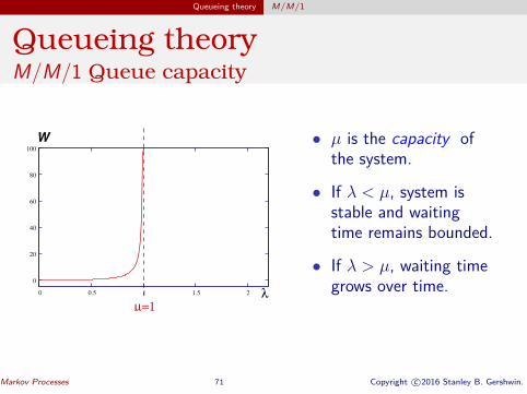
Queueing theory M/M/1
Queueing theoryM/M/1 Queue capacity
W
µ=1
λ
0
20
40
60
80
100
0 0.5 1 1.5 2
• µ is the capacity ofthe system.
• If λ < µ, system isstable and waitingtime remains bounded.
• If λ > µ, waiting timegrows over time.
Markov Processes 71 Copyright ©c 2016 Stanley B. Gershwin.
Page 72
Queueing theory M/M/1
Queueing theoryM/M/1 Queue capacity
W
λ
µ=1
µ=2
0
20
40
60
80
100
0 0.5 1 1.5 2
• To increase capacity,increase µ.
• To decrease delay for agiven λ, increase µ.
Markov Processes 72 Copyright ©c 2016 Stanley B. Gershwin.
Page 73
Queueing theory Other Single-Stage Models
Queueing theoryOther Single-Stage Models
Things get more complicated when:
• There are multiple servers.
• There is finite space for queueing.
• The arrival process is not Poisson.
• The service process is not exponential.
Closed formulas and approximations exist for some, but not all,cases.
Markov Processes 73 Copyright ©c 2016 Stanley B. Gershwin.
Page 74
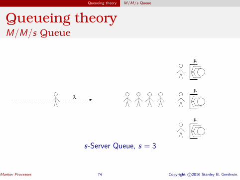
Queueing theory M/M/s Queue
Queueing theoryM/M/s Queue
µ
µ
µ
λ
s-Server Queue, s = 3
Markov Processes 74 Copyright ©c 2016 Stanley B. Gershwin.
Page 75
Queueing theory M/M/s Queue
Queueing theoryM/M/s Queue
µ
λ
µ
λ
0 1 2
µ
λ
µ
λ
µ
λ
µ
λ
µ
λ
2 3
s−1 s
µ
λ
s(s−1) s s(s−2)
s−2 s+1
• The service rate when there are k > s customers in thesystem is sµ since all s servers are always busy.
• The service rate when there are k ≤ s customers in thesystem is kµ since only k of the servers are busy.
Markov Processes 75 Copyright ©c 2016 Stanley B. Gershwin.
Page 76
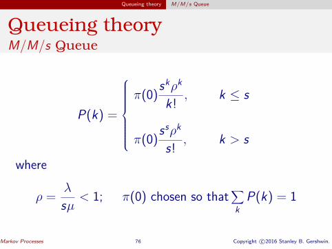
Queueing theory M/M/s Queue
Queueing theoryM/M/s Queue
sk kρ π
P(k) =
(0)k! , k ≤ s
π(0)ssρk
s! , k > s
where
ρ = λ 1;s < π(0) chosen so thatµ
∑P(k) = 1
k
Markov Processes 76 Copyright ©c 2016 Stanley B. Gershwin.
Page 77
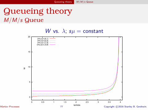
Queueing theory M/M/s Queue
Queueing theoryM/M/s Queue
W vs. λ; sµ = constant
0
5
10
15
20
0 0.5 1 1.5 2 2.5 3 3.5 4
W
lambda
(mu,s)=(4,1)(mu,s)=(2,2)(mu,s)=(1,4)
(mu,s)=(.5,8)
Markov Processes 77 Copyright ©c 2016 Stanley B. Gershwin.
Page 78
Queueing theory M/M/s Queue
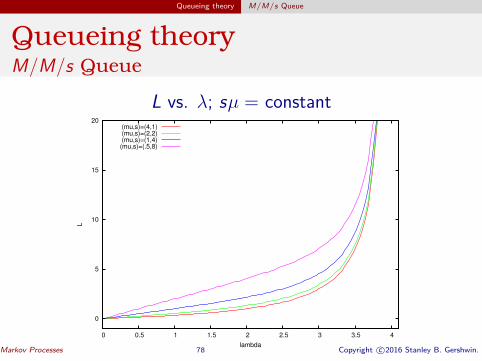
Queueing theoryM/M/s Queue
L vs. λ; sµ = constant
0
5
10
15
20
0 0.5 1 1.5 2 2.5 3 3.5 4
L
lambda
(mu,s)=(4,1)(mu,s)=(2,2)(mu,s)=(1,4)
(mu,s)=(.5,8)
Markov Processes 78 Copyright ©c 2016 Stanley B. Gershwin.
Page 79
Queueing theory M/M/s Queue
Queueing theoryM/M/s Queue
0
5
10
15
20
0 0.5 1 1.5 2 2.5 3 3.5 4
W
lambda
(mu,s)=(4,1)(mu,s)=(2,2)(mu,s)=(1,4)(mu,s)=(.5,8)
0
5
10
15
20
0 0.5 1 1.5 2 2.5 3 3.5 4
L
lambda
(mu,s)=(4,1)(mu,s)=(2,2)(mu,s)=(1,4)(mu,s)=(.5,8)
• Why do all the curves go to infinity at the same value of λ?
• Why does L→ 0 when λ→ 0?
• Why is the (µ, s) = (.5, 8) curve the highest, followed by(µ, s) = (1, 4), etc.?
Markov Processes 79 Copyright ©c 2016 Stanley B. Gershwin.
Page 80
Networks of Queues
Queueing theoryNetworks of Queues
• Set of queues where customers can go to anotherqueue after completing service at a queue.
• Open network: where customers enter and leavethe system. λ is known and we must find L and W .
• Closed network: where the population of thesystem is constant. L is known and we must find λand W .
Markov Processes 80 Copyright ©c 2016 Stanley B. Gershwin.
Page 81
Networks of Queues Examples
Queueing theoryNetworks of Queues
Examples of Open networks
• internet traffic• emergency room• food court• airport (arrive, ticket counter, security, passport
control, gate, board plane)• factory with no centralized material flow control
after material entersMarkov Processes 81 Copyright ©c 2016 Stanley B. Gershwin.
Page 82
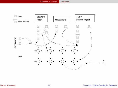
Networks of Queues Examples
PersonSbarro’s TCBY
PIZZA McDonald’s Frozen YogurtPerson with Tray
EN
TR
AN
CE
Tables
EX
IT
Markov Processes 82 Copyright ©c 2016 Stanley B. Gershwin.
Page 83
Networks of Queues Examples
Queueing theoryNetworks of Queues
Examples of Closed networks
• factory with material controlled by keeping thenumber of items constant (CONWIP)
• factory with limited fixtures or pallets
Empty Pallet Buffer
Raw Part Input
Finished Part Output
Markov Processes 83 Copyright ©c 2016 Stanley B. Gershwin.
Page 84
Networks of Queues Jackson Networks
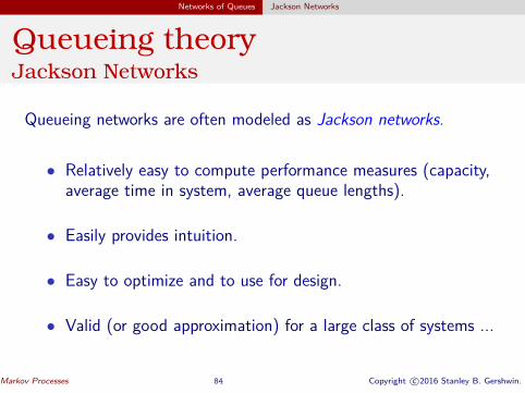
Queueing theoryJackson Networks
Queueing networks are often modeled as Jackson networks.
• Relatively easy to compute performance measures (capacity,average time in system, average queue lengths).
• Easily provides intuition.
• Easy to optimize and to use for design.
• Valid (or good approximation) for a large class of systems ...
Markov Processes 84 Copyright ©c 2016 Stanley B. Gershwin.
Page 85
Networks of Queues Jackson Networks
Queueing theoryJackson Networks
• ... but not all. Storage areas must be infinite (i.e., blockingnever occurs).
? This assumption leads to bad results for systems withbottlenecks at locations other than the first station.
Markov Processes 85 Copyright ©c 2016 Stanley B. Gershwin.
Page 86
Networks of Queues Open Jackson Networks
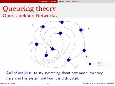
Queueing theoryOpen Jackson Networks
= B M
A
A
A
D
D
Goal of analysis: to say something about how much inventorythere is in this system and how it is distributed.
Markov Processes 86 Copyright ©c 2016 Stanley B. Gershwin.
Page 87
Networks of Queues Open Jackson Networks
Queueing theoryOpen Jackson Networks
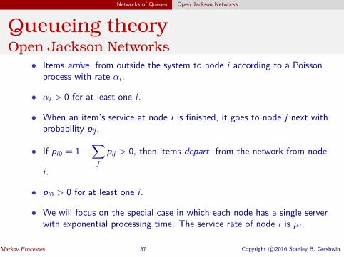
• Items arrive from outside the system to node i according to a Poissonprocess with rate αi .
• αi > 0 for at least one i .
• When an item’s service at node i is finished, it goes to node j next withprobability pij .
• If pi0 = 1−∑
pij > 0, then items depart from the network from nodej
i .
• pi0 > 0 for at least one i .
• We will focus on the special case in which each node has a single serverwith exponential processing time. The service rate of node i is µi .
Markov Processes 87 Copyright ©c 2016 Stanley B. Gershwin.
Page 88
Networks of Queues Open Jackson Networks
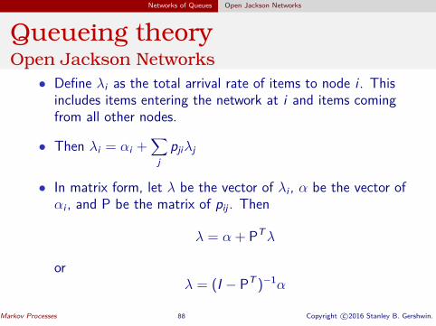
Queueing theoryOpen Jackson Networks• Define λi as the total arrival rate of items to node i . This
includes items entering the network at i and items comingfrom all other nodes.
• Then λi = αi +∑
pjiλjj
• In matrix form, let λ be the vector of λi , α be the vector ofαi , and P be the matrix of pij . Then
= + PTλ α λ
orλ = (I − PT )−1α
Markov Processes 88 Copyright ©c 2016 Stanley B. Gershwin.
Page 89
Networks of Queues Open Jackson Networks
Queueing theoryOpen Jackson Networks
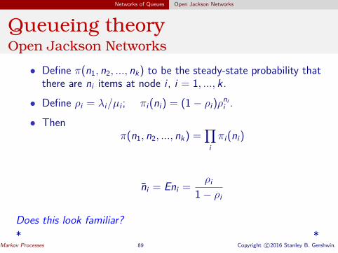
• Define π(n1, n2, ..., nk) to be the steady-state probability thatthere are ni items at node i , i = 1, ..., k .
• Define ρi = nλi/µ ii ; πi(ni) = (1− ρi)ρi .
• Thenπ(n1, n2, ..., nk) =
∏πi(ni)
i
n̄ = En ii = ρ
i 1− ρi
Does this look familiar?* *
Markov Processes 89 Copyright ©c 2016 Stanley B. Gershwin.
Page 90
Networks of Queues Open Jackson Networks
Queueing theoryOpen Jackson Networks
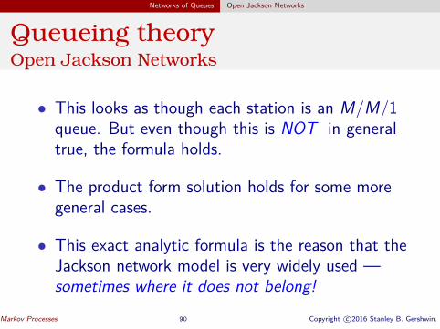
• This looks as though each station is an M/M/1queue. But even though this is NOT in generaltrue, the formula holds.
• The product form solution holds for some moregeneral cases.
• This exact analytic formula is the reason that theJackson network model is very widely used —sometimes where it does not belong!
Markov Processes 90 Copyright ©c 2016 Stanley B. Gershwin.
Page 91
Networks of Queues Closed Jackson Networks
Queueing theoryClosed Jackson Networks
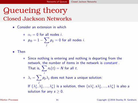
• Consider an extension in which
? αi = 0 for∑all nodes i .? pi0 = 1− pij = 0 for all nodes i .
j
• Then
? Since nothing is entering and nothing is departing from thenetwork,∑the number of items in the network is constant .That is, ni (t) = N for all t.
? λi =∑ i
pjiλj does not have a unique solution:j
If {λ∗1 , λ
∗2 , ..., λ
∗k} is a solution, then {sλ∗
1 , sλ∗2 , ..., sλ∗
k} is also asolution for any s ≥ 0.
Markov Processes 91 Copyright ©c 2016 Stanley B. Gershwin.
Page 92
Networks of Queues Closed Jackson Networks
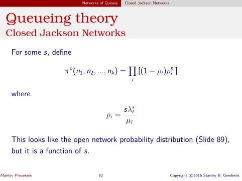
Queueing theoryClosed Jackson Networks
For some s, define
oπ (n1, n2, ..., n nik) =
∏[(1
i− ρi)ρi ]
where
s iρ = λ∗i
µi
This looks like the open network probability distribution (Slide 89),but it is a function of s.
Markov Processes 92 Copyright ©c 2016 Stanley B. Gershwin.
Page 93
Networks of Queues Closed Jackson Networks
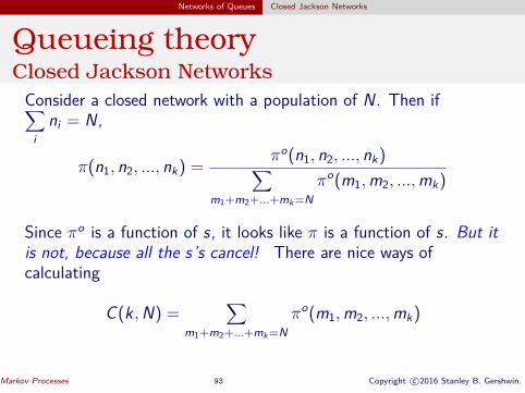
Queueing theoryClosed Jackson Networks
Consider a closed network with a population of N . Then if∑ni = N ,
io
π(n1, n2, ..., nk) = π (n1, n2, ..., nk)o
m1+m2+
∑π (m1,m2, ...,mk)
...+mk=N
Since oπ is a function of s, it looks like π is a function of s. But itis not, because all the s’s cancel! There are nice ways ofcalculating
C(k ,N) =∑ oπ (m1,m2, ...,mk)
m1+m2+...+mk=N
Markov Processes 93 Copyright ©c 2016 Stanley B. Gershwin.
Page 94
Networks of Queues Application — Simple Flexible Manufacturing System model
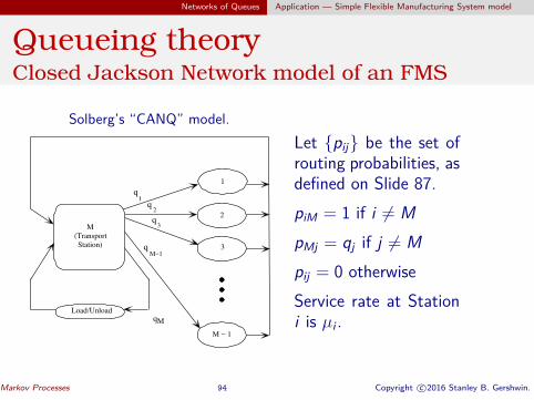
Queueing theoryClosed Jackson Network model of an FMS
Solberg’s “CANQ” model.
M
(Transport
Station)
Load/Unload
M − 1
3
2
1
q1
2
3
M−1q
q
q
qM
Let {pij} be the set ofrouting probabilities, asdefined on Slide 87.piM = 1 if i 6= MpMj = qj if j 6= Mpij = 0 otherwiseService rate at Stationi is µi .
Markov Processes 94 Copyright ©c 2016 Stanley B. Gershwin.
Page 95
Networks of Queues Application — Simple Flexible Manufacturing System model
Queueing theoryClosed Jackson Network model of an FMS
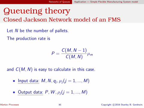
Let N be the number of pallets.The production rate is
C(MP = ,N − 1)C(M,N) µm
and C(M,N) is easy to calculate in this case.
• Input data: M,N , qj , µj(j = 1, ...,M)
• Output data: P,W , ρj(j = 1, ...,M)
Markov Processes 95 Copyright ©c 2016 Stanley B. Gershwin.
Page 96
Networks of Queues Application — Simple Flexible Manufacturing System model
Queueing theoryClosed Jackson Network model of an FMS
P
Number of pallets
0.05
0.1
0.15
0.2
0.25
0.3
0.35
0 2 4 6 8 10 12 14 16 18 20
Markov Processes 96 Copyright ©c 2016 Stanley B. Gershwin.
Page 97
Networks of Queues Application — Simple Flexible Manufacturing System model
Queueing theoryClosed Jackson Network model of an FMS
Average time in system
Number of Pallets
10
20
30
40
50
60
70
0 2 4 6 8 10 12 14 16 18 20
Markov Processes 97 Copyright ©c 2016 Stanley B. Gershwin.
Page 98
Networks of Queues Application — Simple Flexible Manufacturing System model
Queueing theoryClosed Jackson Network model of an FMS
Utilization
Station 2
Number of Pallets
0
0.2
0.4
0.6
0.8
1
0 2 4 6 8 10 12 14 16 18 20
Markov Processes 98 Copyright ©c 2016 Stanley B. Gershwin.
Page 99
Networks of Queues Application — Simple Flexible Manufacturing System model
Queueing theoryClosed Jackson Network model of an FMS
P
Station 2 operation time
0.2
0.25
0.3
0.35
0.4
0.45
0.5
0.55
0.6
0 0.5 1 1.5 2 2.5 3 3.5 4 4.5 5
Markov Processes 99 Copyright ©c 2016 Stanley B. Gershwin.
Page 100
Networks of Queues Application — Simple Flexible Manufacturing System model
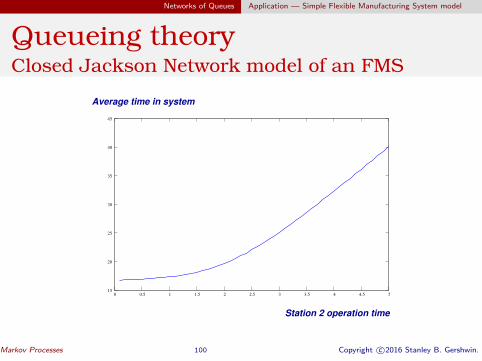
Queueing theoryClosed Jackson Network model of an FMS
Average time in system
Station 2 operation time
15
20
25
30
35
40
45
0 0.5 1 1.5 2 2.5 3 3.5 4 4.5 5
Markov Processes 100 Copyright ©c 2016 Stanley B. Gershwin.
Page 101
Networks of Queues Application — Simple Flexible Manufacturing System model
Queueing theoryClosed Jackson Network model of an FMS
Utilization
Station 2
Station 2 operation time
0
0.2
0.4
0.6
0.8
1
0 0.5 1 1.5 2 2.5 3 3.5 4 4.5 5
Markov Processes 101 Copyright ©c 2016 Stanley B. Gershwin.
Page 102
MIT OpenCourseWarehttps://ocw.mit.edu
2.854 / 2.853 Introduction To Manufacturing SystemsFall 2016
For information about citing these materials or our Terms of Use, visit: https://ocw.mit.edu/terms.